SparseAuto: An Auto-Scheduler for Sparse Tensor Computations Using Recursive Loop Nest Restructuring

Abstract.

Automated code generation and performance enhancements for sparse tensor algebra have become essential in many real-world applications, such as quantum computing, physical simulations, computational chemistry, and machine learning. General sparse tensor algebra compilers are not always versatile enough to generate asymptotically optimal code for sparse tensor contractions. This paper shows how to generate asymptotically better schedules for complex sparse tensor expressions using kernel fission and fusion. We present generalized loop restructuring transformations to reduce asymptotic time complexity and memory footprint.

Furthermore, we present an auto-scheduler that uses a partially ordered set (poset)-based cost model that uses both time and auxiliary memory complexities to prune the search space of schedules. In addition, we highlight the use of Satisfiability Module Theory (SMT) solvers in sparse auto-schedulers to approximate the Pareto frontier of better schedules to the smallest number of possible schedules, with user-defined constraints available at compile-time. Finally, we show that our auto-scheduler can select better-performing schedules and generate code for them. Our results show that the auto-scheduler provided schedules achieve orders-of-magnitude speedup compared to the code generated by the Tensor Algebra Compiler (TACO) for several computations on different real-world tensors.

1. Introduction

Tensor contractions – a generalization of matrix multiplications – are used in many real-world applications including, but not limited to physical simulations, machine learning, computational chemistry, and quantum computing (Hirato, [n. d.]; Markov, 2008; Ran et al., 2020; Kossaifi et al., 2017; Ran et al., 2017). When most of the values in these tensors become zero, it is advantageous to use compressed representations to store only the non-zero values, and such tensors are known as Sparse Tensors. Sparse tensors contractions can exploit zero values by skipping computations over them (i.e., x + 0 = x and x * 0 = 0). Many important applications such as Graph Neural Networks (GNN), Physical Simulation, and Quantum Chemistry (Hamilton et al., 2017; Hu et al., 2020; Rahman et al., 2021) make use of sparse tensor contractions.

There are several challenges associated with sparse tensor contractions: (i) These computations are consolidated using loop nests, some of which are non-affine in nature due to compressed data formats (Section 2.1) used to store sparse tensors; (ii) the special data structures used in storing sparse tensors introduce complexities, such as load imbalances and data locality issues, into sparse tensor contractions; (iii) there are multiple ways to achieve the same computation by using transformations like loop reordering, loop fusion/fission, blocking/tiling, splitting, unrolling, parallelization, vectorization, etc. (Senanayake et al., 2020), and it is hard to decide which ones to apply. Prior works (Kjolstad et al., 2017a; Bik and Wijshoff, 1993; Tian et al., 2021a; Venkat et al., 2015; Kotlyar et al., 1997; Senanayake et al., 2020; Bik et al., 2022) have introduced sparse compilers and compiler optimizations to overcome the challenges but there is still room for improvement.

Generating a good schedule for a given sparse tensor contraction is not straightforward as there may be thousands of schedules to choose from (Section 2.4). A good schedule can be found for dense computations given the loop bounds and the specification of the machine that is used to execute the computation. For sparse computations, a good schedule selection also depends on the number of non-zero values and the sparsity structure of the sparse tensors. The easiest method to evaluate the cost of a schedule is to execute the schedule on a given machine on given sparse inputs to measure the time it takes to finish execution. However, it is a time-consuming arduous process, hence impractical, to evaluate all the schedules to find the best schedule. The selection of a good schedule is difficult without evaluating all the schedules for several reasons: (i) accurate and complete modeling of cache and other machine parameters is hard; (ii) the schedule space can be quite large and it may not be possible to explore the entire schedule space within a given time; (iii) sparse computations have non-affine loops, different sparsities and sparsity structures for different tensors. Hence, a schedule explorer must settle into using heuristics (e.g. the number of memory accesses, the number of floating point operations, buffer sizes, etc.) in making decisions about how good a schedule is compared to another schedule. One schedule may not be the best for all the inputs and machines.

We can simplify the problem of finding a good schedule by addressing the above challenges as follows. (i) Since accurate modeling of the machine parameters is hard and can vary from machine to machine, a performance engineer can focus on machine-independent heuristics like the time complexity and auxiliary memory requirements of a schedule, and the program transformations most relevant to these metrics, in particular, loop reordering and loop/kernel fusion/fission. (ii) A performance engineer can prune the large schedule space at compile time by using those machine-independent heuristics and keep a handful of schedules to be evaluated at runtime. (iii) A performance engineer can incorporate known information about sparse inputs in reasoning to help them with the pruning process. Based on these points, this paper introduces an auto-scheduler that uses partially ordered sets (posets) based on time complexity and auxiliary memory complexity for schedule selection. (Section 5) The existing sparse tensor schedule explorers do not optimize for both time and auxiliary memory complexities (Ahrens et al., 2022; Kanakagari and Solomonik, 2023).

Since loop fusion and fission mainly dictate the time complexity and auxiliary memory requirement of a sparse tensor contraction, let’s consider this example of sparse tensor times matrix contraction: $A_{lmn}=\sum_{ijk}\>{{\textbf{{B}}}_{ijk}}\>C_{il}\>D_{jm}\>E_{kn}$ . This computation can be expressed using a simple linear loop nest with a time complexity of $O(nnz({{\textbf{{B}}}_{ijk}})LMN)$. Alternatively, it can be expressed as $T_{ijn}=\sum_{k}\>B_{ijk}\>E_{kn}$ and $A_{lmn}=\sum_{ij}\>T_{ijn}\>C_{il}\>D_{jm}$ – two separate computations with a total time complexity of $O(nnz({{\textbf{{B}}}_{ijk}})N+IJNLM)$ and a dense temporary $T$. Since $T$ is 3 dimensional, it can be large. Finally, another way to structure the same computation comes out of an observation that outer loops of the $1^{st}$ computation (producer) can be fused with the $2^{nd}$ computation (consumer). This approach reduces the time complexity to $O(N(nnz({{\textbf{{B}}}_{ijk}})+nnz({{\textbf{{B}}}_{ij}})LM))$  and auxiliary memory to a scalar memory, which is superior to both of the previous versions asymptotically. This stems from the fact that the loop structure of the schedule is not a simple loop nest, and there could exist other schedules that have multi-level branching in their loop structure which do not dominate the time and auxiliary memory complexities as explained in Section 3.

This paper introduces a scheduling directive and an extended representation of branched iteration graphs that can be used to generate schedules with multi-level branching in their loop structure to reduce the time complexity and auxiliary memory requirements of a tensor contraction (Section 4). Furthermore, we explore the schedule space of a given sparse tensor computation and present strategies based on posets that can be combined with user-given constraints at compile time to prune the schedule space (Section 5). Our specific contributions are:

Recursive extension of branched iteration graph:

We generalize the branched iteration graph (BIR) intermediate representation of SparseLNR to support multiple levels of imperfectly nested loops and recursive fusion/fission.

New scheduling primitives:

We introduce a new scheduling primitive for the recursive application of loop fusion and fission into the BIR and extend the existing loop reorder primitive to enable their application on nested loops.

Poset-based auto-scheduler:

We introduce a novel poset-based auto-scheduler that uses both time and auxiliary memory complexities to prune the schedule space.

An SMT solver-based pruning of space:

We highlight the importance of pruning the schedule space at compile time with user-defined constraints using an SMT solver and posets.

Section 3 motivates the problem, Section 4 introduces the multi-level branched iteration graph and the scheduling primitives, and Section 5 describes the poset-based auto-scheduler. Finally, we show that our auto-scheduler selects schedules that outperform TACO-generated schedules by orders of magnitude in Section 6.

2. Background

This section provides the necessary background on tensor tensor contractions, level formats, the concept of iteration graphs, and scheduling primitives.

2.1. Level Formats for Sparse Tensors

There are several compressed data formats used to store sparse tensors, Compressed Sparse Row (CSR), Compressed Sparse Column (CSC), Sorted Coordinate (Sorted COO), Compressed Sparse Fiber (CSF), Doubly Compressed Sparse Row (DCSR), etc to name a few. These formats are called level formats because they are tree-like structures and index arrays need to be traversed one after the other to finally access the values. For example, if ${{\textbf{{A}}}{ij}}$ is in CSR format, then $i$ needs to be accessed first to access the $j$ index array, and then the value of ${{\textbf{{A}}}{ij}}$. We call them sparse index constraints in the paper because they impose constraints on the ways the loops can be reordered in a sparse tensor contraction. Chou et al.  (Chou et al., 2018) describes the level formats in detail. We will limit the study in this paper to level formats.

2.2. Tensor Index Notation for Tensor Contractions

The notation used to describe tensor contraction operations is based on the Einstein summation convention. The Einstein summation convention is a notational convention that implies summation over a set of repeated indices. For example, the expression $X(i,k)=A(i,j)\cdot B(j,k)$ implies summation over the repeated index $j$ and would be equivalent to the standard mathematical notation $A_{jk}=\sum\nolimits_{j}B_{ij}C_{jk}$. We use both these notations interchangeably in the texts. Since this computation can be performed using a simple linear triply nested loop, we say that the iteration time complexity of this computation is $O(IJK)$. If $B$ is sparse, then the iteration time complexity is $O(nnz({{\textbf{{B}}}_{ij}})K)$. Here, nnz is the number of non-zero elements.

2.3. Iteration Graph

Kjolstad et al.  (Kjolstad et al., 2017a) describes the concept of iteration graphs in detail. We will summarize it here for completeness. Take the sparse tensor times matrix multiplication (TTMC), $A_{lmn}=\sum_{ijk}\>{{\textbf{{B}}}_{ijk}}\>C_{il}\>D_{jm}\>E_{kn}$, as an example. An iterator that iterates through all of $i$, $j$, $k$, $l$, $m$, and $n$, can read each value of ${{\textbf{{B}}}_{ij}}$, $C_{il}$, $D_{jm}$, $E_{kn}$, multiply them and store the result in $A_{lmn}$. An example iteration graph is shown in Figure 2(b) and this internal representation (IR) is then later used to generate Code 1(a). In the iteration graph, nodes represent indices in the Einsum notation. This is an acyclic graph where the edges represent the dimensions in tensors and how they map to indices. Since $B$ is sparse, $B_{1}$, $B_{2}$, and $B_{3}$ incidenting on indices $i$, $j$, and $k$ should appear in that order. Since all the other tensors are dense, other indices can appear in any order. $C_{2}$ can appear before $C_{1}$ because $C$ is a dense matrix and there are no sparsity constraints imposed by the level formats described in Section 2.1.

2.4. Scheduling Primitives

There are multiple ways to achieve the same computation. For example, we can change the loop order in Code 1(a) to have the order $l,i,m,j,n,k$ instead of $l,m,n,i,j,k$. A schedule describes one way of expressing the computation. Kjolstad et al.  (Kjolstad et al., 2017a) and Senanayake (Senanayake et al., 2020) describe the importance of having a separation of concern between computation (what) and schedule (how). They introduce scheduling primitives to describe the schedule. Some of the scheduling primitives are as follows: split directive to split a loop for tiling, collapse to collapse one loop onto another, reorder to reorder the loops, parallelize and vectorize for parallel execution. Kjolstad et al.  (Kjolstad et al., 2019) introduces precompute to add dense workspaces to remove sparse accesses.

In Section 4, we will introduce a new scheduling primitive called loopfuse that can be used to produce loop nests with multiple loop nest branches in combination with the reorder directive.

3. Overview

It may not be straightforward to decide whether or not to apply transformations across multiple kernels. The decision depends both on the iteration complexity of the final loop nests and the working set sizes. If the working set sizes are small and fit into the cache then, it is better to use the version with lower iteration complexity. Otherwise, it is better to use the schedule with lower auxiliary memory. Hence, an auto-scheduler that only looks at the iteration complexity or only the auxiliary memory complexity may choose the wrong schedule as the final output or prune a good schedule from the search space in the process.

⬇ 1 for (int32_t l, m, n, i;; l++, m++, n++, i++) { 2 for (int32_t jB = B2_pos[i]; jB < B2_pos[i+1]; jB++) { 3 int32_t j = B2_crd[jB]; 4 for (int32_t kB = B3_pos[j]; kB < B3_pos[j+1]; kB++) { 5 int32_t k = B3_crd[kB]; 6 A(l,m,n) += B(i,j,k) * C(i,l) * D(j,m) * E(k,n); 7 } 8 } 9 }

(a) ${A_{lmn}}=\sum\nolimits_{ijk}{{\textbf{{B}}}_{ijk}}\cdot C_{il}\cdot D_{jm}\cdot E_{kn}$
Time: $O(LMN\cdot nnz(B))$
 $Memory:0$

[C++ code of the kernel sampled dense-dense matrix multiplication kernel]¡long description¿

⬇ 1 for (int32_t l, m; ; l++, m++) { 2 float T<K> = 0.0; 3 for (int32_t i; ; i++) { 4 for (int32_t jB = B2_pos[i]; jB < B2_pos[i+1]; jB++) { 5 int32_t j = B2_crd[jB]; 6 for (int32_t kB = B3_pos[j]; kB < B3_pos[j+1]; kB++) { 7 int32_t k = B3_crd[kB]; 8 T(k) += B(i,j,k) * C(i,l) * D(j,m); 9 } 10 } 11 } 12 for (int32_t n,k; ; n++, k++) { 13 A(l,m,n) += T(k) * E(k,n); 14 } 15 }

(b) ${A_{lmn}}=\sum\nolimits_{k}(\sum\nolimits_{ij}{{\textbf{{B}}}_{ijk}}\cdot C_{il}\cdot D_{jm})\cdot E_{kn}$
Time: $O(LM\cdot(nnz(B)+NK))$
 $Memory:K$

[C++ code of the sparse matrix multiplication kernel]¡long description¿

⬇ 1 for (int32_t l; ; l++) { 2 float T<J, K> = 0.0; 3 for (int32_t i; ; i++) { 4 for (int32_t jB = B2_pos[i]; 5 jB < B2_pos[i+1]; jB++) { 6 int32_t j = B2_crd[jB]; 7 for (int32_t kB = B3_pos[j]; 8 kB < B3_pos[j+1]; kB++) { 9 int32_t k = B3_crd[kB]; 10 T(j,k) += B(i,j,k) * C(i,l); 11 } 12 } 13 } 14 for (int32_t m,k; ; m++, k++) { 15 float t = 0.0; 16 for (int32_t j; ; j++) { 17 t += T(j,k) * D(j,m); 18 } 19 for (int32_t n; ; n++) { 20 A(l,m,n) += t * E(k,n); 21 } 22 } 23 }

(c) ${A_{lmn}}=\sum\nolimits_{k}(\sum\nolimits_{j}(\sum\nolimits_{i}{{\textbf{{B}}}_{ijk}}\cdot C_{il})\cdot D_{jm})\cdot E_{kn}$
$Time:O(L\cdot(nnz(B)+MK\cdot(J+N)))$
 $Memory:KJ$

[C++ code of the kernel fused sampled dense-dense matrix multiplication kernel and sparse matrix multiplication kernel]¡long description¿

⬇ 1 for (int32_t l; ; l++) { 2 float T<J, K> = 0.0; 3 for (int32_t i; ; i++) { 4 for (int32_t jB = B2_pos[i]; 5 jB < B2_pos[i+1]; jB++) { 6 int32_t j = B2_crd[jB]; 7 for (int32_t kB = B3_pos[j]; 8 kB < B3_pos[j+1]; kB++) { 9 int32_t k = B3_crd[kB]; 10 T(j,k) += B(i,j,k) * C(i,l); 11 } 12 } 13 } 14 for (int32_t m; ; m++) { 15 float T2<K> = 0.0; 16 for (int32_t j, k; ; j++, k++) { 17 T2(k) += T(j,k) * D(j,m); 18 } 19 for (int32_t n, k; ; n++, k++) { 20 A(l,m,n) += T2(k) * E(k,n); 21 } 22 } 23 }

(d) ${A_{lmn}}=\sum\nolimits_{k}(\sum\nolimits_{j}(\sum\nolimits_{i}{{\textbf{{B}}}_{ijk}}\cdot C_{il})\cdot D_{jm})\cdot E_{kn}$
$Time:O(L\cdot(nnz(B)+MK\cdot(J+N)))$
$Memory:KJ+K$

[C++ code of the kernel fused sampled dense-dense matrix multiplication kernel and sparse matrix multiplication kernel]¡long description¿

⬇ 1 for (int32_t l; ; l++) { 2 float T<J, K> = 0.0; 3 for (int32_t i; ; i++) { 4 for (int32_t jB = B2_pos[i]; 5 jB < B2_pos[i+1]; jB++) { 6 int32_t j = B2_crd[jB]; 7 for (int32_t kB = B3_pos[j]; 8 kB < B3_pos[j+1]; kB++) { 9 int32_t k = B3_crd[kB]; 10 T(j,k) += B(i,j,k) * C(i,l); 11 } 12 } 13 } 14 for (int32_t m, n, j, k; ; m++, n++, j++, k++) { 15 A(l,m,n) += T(j,k) * D(j,m) * E(k,n); 16 } 17 }

(e) ${A_{lmn}}=\sum\nolimits_{jk}(\sum\nolimits_{i}{{{\textbf{{B}}}_{ijk}}\cdot C_{il}})\cdot D_{jm}\cdot E_{kn}$
$Time:O(L\cdot(nnz(B)+JMKN))$
$Memory:KJ$

[C++ code of the kernel fused sampled dense-dense matrix multiplication kernel and sparse matrix multiplication kernel]¡long description¿

Figure 1. Different schedules of executing ${A_{lmn}}=\sum\nolimits_{ijk}{{\textbf{{B}}}_{ijk}}\cdot C_{il}\cdot D_{jm}\cdot E_{kn}$. Here, the code snippet 1(a) has a perfectly nested loop structure while all the other code snippets have imperfectly nested loop structures. The code snippets 1(b) and 1(e) have one level of branching whereas the code snippets 1(c) and 1(d) have two levels of branching.

3.1. Motivating Example

Consider the following tensor contraction of a sparse 3D tensor with three matrices to produce another 3D tensor, $A(l,m,n)={{\textbf{{B}}}(i,j,k)}\cdot C(i,l)\cdot D(j,m)\cdot E(k,n)$. We can think of several schedules to perform this computation. Figure 1(a) refers to performing the computation using a simple loop nest of depth 6. The same computation can be written as in figures 1(b), 1(c), 1(d) and 1(e) with branching loop nests of depth 4 or 5. In this section, we will discuss the performance of these different schedules. We will evaluate all the schedules with the same loop structure, but with different index ordering and report the best one. For the loop structure in Figure 1(c), we will evaluate both the inner loop order of $m,k$ and $k,m$. Similarly for Figure 1(b), we will evaluate four different loop orders, two of them by interchanging the inner loops $n,k$ and two of them by interchanging the outer loops $l,m$.

From an asymptotic time complexity perspective, an auto-scheduler might lean towards discarding or pruning the Schedule 1(a). This is due to its loop nesting depth of 6 and asymptotic time complexity of $O(nnz(B_{IJK})LMN)$, in contrast to the schedule in Figure 1(b) with a loop nesting depth of 5 and asymptotic time complexity of $O(nnz(B_{IJK})LM+LMNK)$ or the schedule in Figure 1(c) with a loop nesting depth of 4 and asymptotic time complexity of $O(nnz(B_{IJK})L+LMK(J+N))$. Notably, the schedule in Figure 1(d) has the same asymptotic time complexity as the schedule in Figure 1(c), while the asymptotic time complexity of the schedule in Figure 1(e) is $O(nnz(B_{IJK})L+LJMKN)$.

From an asymptotic time complexity viewpoint, an auto-scheduler may tend to choose either the schedule in Figure 1(c) or the schedule in Figure 1(d) because it has a loop depth of 4, lowest out of all five schedules in Figure 1. If we compare schedules in Figures 1(c) and 1(d), we see that one 2D auxiliary memory is used to store intermediate results between the branched loop nests in the former, whereas a 2D and a 1D auxiliary pieces of memory are used in the later. Hence, the schedule first has a lower memory complexity compared to the second schedule. We say that the schedule in Figure 1(c) dominates the schedule in Figure 1(d), because both the schedules have the same asymptotic time complexity, but the first schedule is better in terms of the auxiliary memory complexity.

If we compare the schedules in Figures 1(c) and 1(e), we see that both the schedules have an auxiliary memory complexity of $O(KJ)$. The asymptotic time complexity of the schedule in Figure 1(c) would be better since $O(J+N)$ is better than $O(JN)$ for larger values of $J$ and $N$. Therefore, we say that the schedule in Figure 1(c) dominates the schedule in Figure 1(e). Hence, for the comparisons mentioned in the below paragraphs, we omit the comparison of the schedules in Figures 1(d) and 1(e) with the other schedules.

Consider the comparison of the schedules in Figures 1(a), 1(b), and 1(c) when the bounds change in the range as follows; $1<=I<=1800$, $1<=J<=1600$, $400<=K<=4000$, $8<=L<=256$, $8<=M<=256$, $8<=N<=256$, and $0.001<=sparsity(B)<=0.01$. Note that the schedule in Figure 1(a) does not dominate both the schedules in Figures 1(b) and 1(c) in terms of the auxiliary memory usage because no auxiliary memory is used in the Schedule 1(a). Although the loop depth is four for the schedule in Figure 1(c), within the given ranges of bounds and the sparsity of $B$, we cannot claim that it is the best in all cases. Let us look at some cases by changing the loop bounds and sparsity for tensor B. The evaluation configuration is explained in the Section 6.

Case ①

In this case, we set the loop bounds for the schedules in Figure 1 to specific values: $I=1800$, $J=800$, $K=1000$, $L=64$, $M=16$, $N=32$, and $sparsity(B)=0.08$. Under these conditions, the iteration time complexities are determined as $\Phi(b)\thickapprox 7.5*\Phi(c)$   and $\Phi(a)\thickapprox 237.5*\Phi(c)$. The corresponding execution times are $\Psi(a)=32.40s$ , $\Psi(b)=6.26s$, and $\Psi(c)=2.48s$. The schedule in Figure 1(c) exhibits the lowest loop depth and iteration time complexity, while the schedule in Figure 1(c) demands an auxiliary memory of 3.05MB and the schedule in Figure 1(b) requires 3.91KB. An auto-scheduler that factors in loop depth could choose the best schedule in this case.

Case ②

Adjusting the loop bounds to $J=1600$, $K=2000$ and $sparsity(B)=0.02$ while maintaining other loop bounds as in the previous example, the iteration time complexities shift: $\Phi(b)\thickapprox 3*\Phi(c)$ and $\Phi(a)\thickapprox 92.5*\Phi(c)$. The schedule in Figure 1(c), with the minimum loop depth, exhibits the lowest iteration time complexity as before. Execution times for the schedules are $\Psi(a)=33.51s$, $\Psi(b)=8.60s$, and $\Psi(c)=10.20s$. The schedule in Figure 1(c) maintains the lowest iteration time complexity, but the schedule in Figure 1(b), with a loop depth of 5, performs better. The schedule in Figure 1(c) now incurs an auxiliary temporary memory requirement of $12.21MB$ compared to the previous $3.05MB$. This consumes more than $50\%$ of the Last-Level-Cache (LLC). Consequently, an auto-scheduler solely reliant on loop depth would fail in this scenario. A robust auto-scheduler must consider both iteration time complexity and auxiliary memory requirements to make informed decisions about schedule selection or pruning schedules from the search space.

Case ③

Now we set the values of the loop bounds and the sparsity as follows: $I=265$, $J=1207$, $K=479$, $L=251$, $M=234$, $N=42$, and $sparsity(B)\approx 0.0033$. Under these conditions, the schedule in Figure 1(b) exhibits the fastest execution time of $\Psi(b)=513ms$, while the schedule in Figure 1(c) completed in $\Psi(c)=1.14s$, and the schedule in Figure 1(a) requires $\Psi(a)=1.66s$. The auxiliary memory usage for the schedule in Figure 1(c) is $2.21MB$, whereas that of the schedule in Figure 1(b) is a mere $1.87KB$. Both of the schedules’ auxiliary memories account for less than $12\%$ of the LLC. For these specified values, $\Phi(a)=1.13*\Phi(b)$ and $\Phi(c)=40.4*\Phi(b)$. The execution times align with the iteration time complexities of each schedule, and the auxiliary memory usage is reasonably modest. In contrast to Cases ① and ②, the schedule with neither the best loop depth nor the best auxiliary memory depth proves to be the most efficient one. This instance underscores the importance for schedulers to consider factors beyond the loop depth and auxiliary memory depth when making informed decisions about pruning the search space.

Conclusions from the cases

The conclusions from the experiments of cases are as follows;

1. Loop depth alone is not a good indicator of the performance of the schedules. Even the schedule with the highest loop depth (e.g., Case ②) or some other schedule (e.g., Case ③) can perform better than the schedule with minimum loop depth.

2. Loop depth and auxiliary memory requirement are both important factors in deciding the performance of the schedules (e.g., Case ①).

3. If the auxiliary memory requirement takes up a large portion of the LLC, then that schedule tends to perform worse than the other schedules (e.g., Case ②).

3.2. Our approach: SparseTDA

Existing languages do not support multi-level branched loop nests, to the best of our knowledge. We extend the scheduling language to support recursive fusion/fission. Furthermore, we introduce an auto-scheduler for selecting schedules using the partial order of time and auxiliary memory complexities. We make the following changes to TACO and SparseLNR and introduce a new auto-scheduler:

1. We extend the branched iteration graph to support recursive, multi-level branched iteration graphs with multi-dimensional temporary buffers.

2. We extend the scheduling language to support the recursive fusion and adapt TACO’s code generation strategies to reflect it.

3. We introduce an auto-scheduler that reasons about the partial orders of time and auxiliary memory complexities using a Satisfiability Modulo Theory (SMT) solver provided with user-defined constraints to prune the search space.

4. Detailed Design of the Transformation

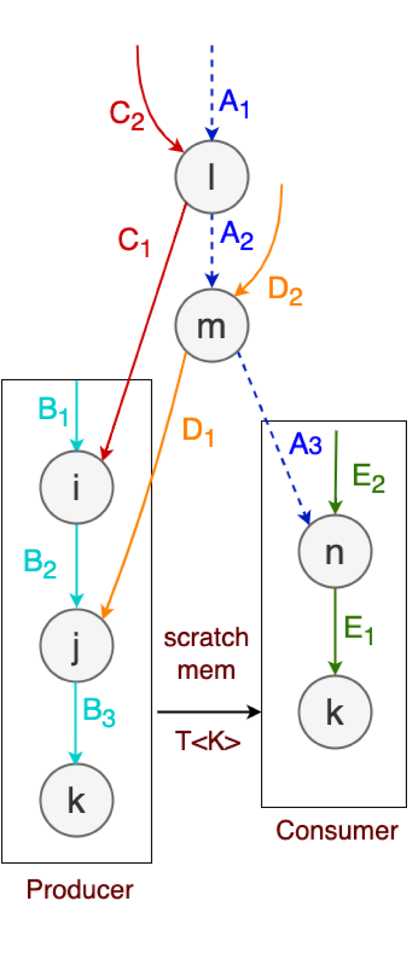
(a) Fused kernel with k extra memory

[Original iteration graph of sddmm spmm operation]¡long description¿

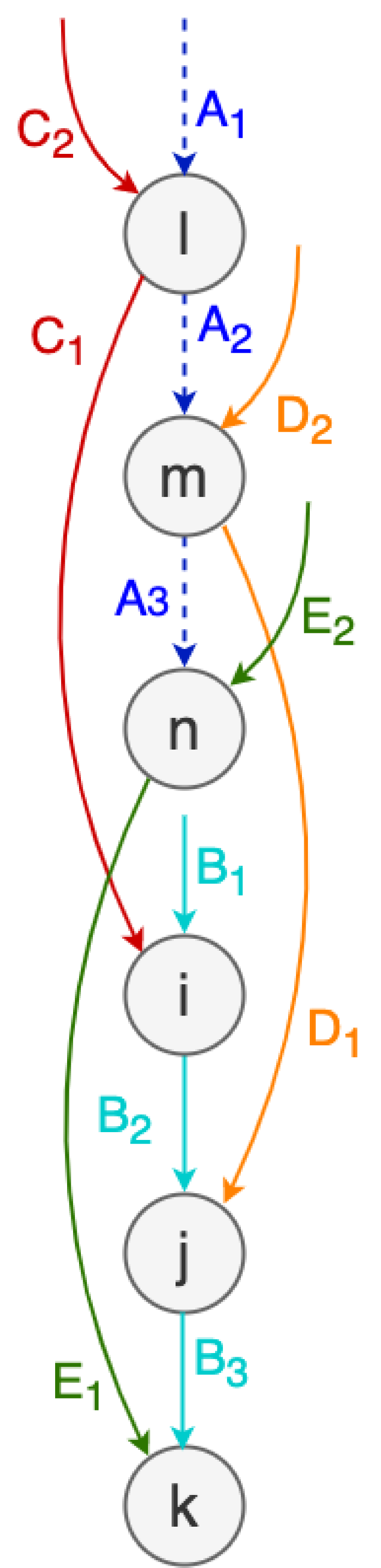
(b) TACO default kernel

[Original iteration graph of sddmm spmm operation]¡long description¿

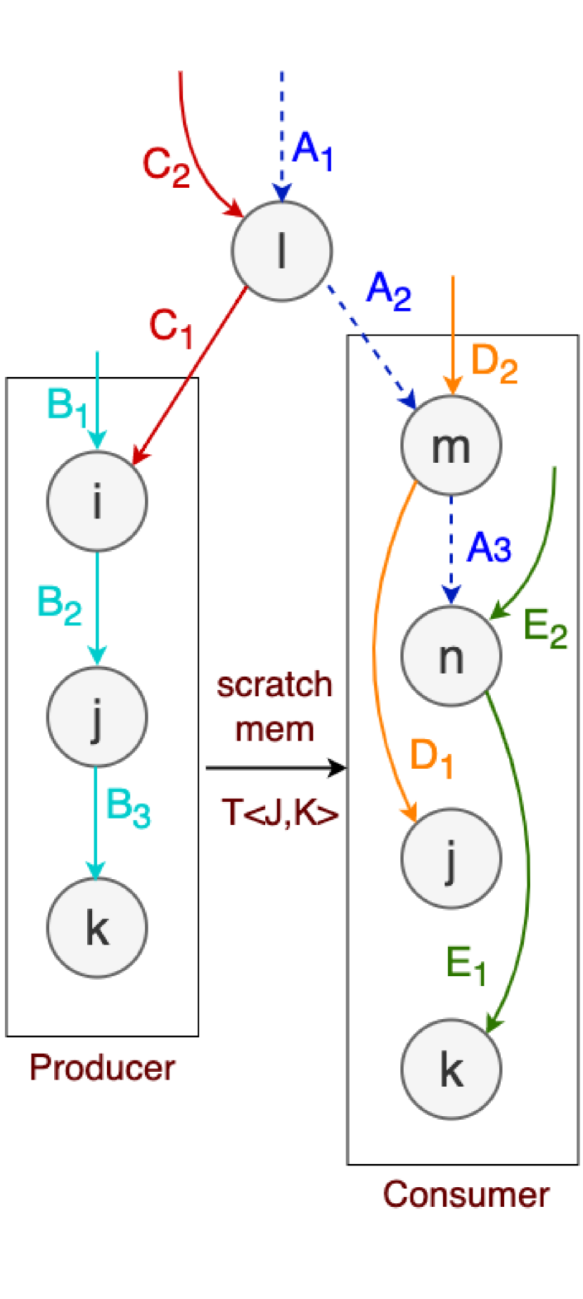
(c) Fused kernel with $JK$ extra memory

[Original iteration graph of sddmm spmm operation]¡long description¿

(d) 2(c) with reordered consumer branch

[Original iteration graph of sddmm spmm operation]¡long description¿

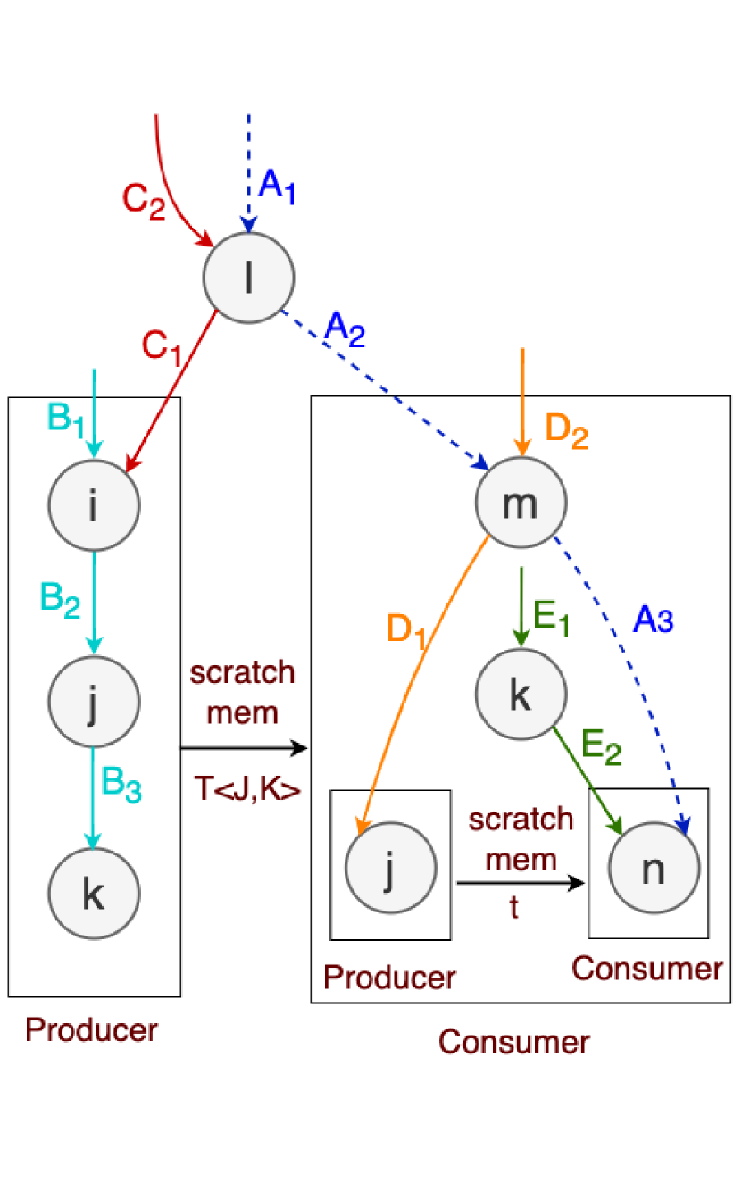
(e) Multi-level nesting after fusing inner branch of 2(d)

[Original iteration graph of sddmm spmm operation]¡long description¿

Figure 2. loopfuse transformation performed on $A_{lmn}=\sum\nolimits_{ijk}{{\textbf{{B}}}_{ijk}}C_{il}D_{jm}E_{kn}$

Tensor contractions can be materialized using a simple linear loop nest where there would be a corresponding loop for each of the indices in the einsum expression. This simple linear loop nest is represented as a linear iteration graph (LIG) as explained in Section 2.3, which is in turn used for sparse code generation. However, this simple loop nest must respect the sparse index order constraints of the sparse tensor. For example, if a sparse tensor is in compressed sparse row format, the row should be accessed first.

In this section, we describe an algorithm to recursively generate a branched iteration graph, the transformation required to convert a LIG into a multi-level branched iteration graph, and how this transformation can cover a plethora of possible loop trees for the computation.

4.1. Equivalence Class of Tensor Contractions

Let us look at the tensor contraction:

$$O(out\_idx)=\displaystyle\sum_{c\_idx}I_{1}(in_{1}\_idx)*\dots*I_{e}(in_{e}\_idx)$$

Here, $I_{1}$, $I_{2}$, etc. denote the input tensors. $O$ denotes the output tensor. $c\_idx$ denotes the indexes that need to be contracted from the tensor expression. This tensor contraction can be materialized using a LIG as in the code snippet 3.

⬇ 1 $loop_{1}$: 2 $\ldots$ 3 $loop_{i}$: 4 $\ldots$ 5 $loop_{j}$: 6 $\ldots$ 7 ${{\textbf{{l}}}oop_{n}}$: 8 $\displaystyle O$ += 9 $\displaystyle I_{1}*..*I_{l}*..*I_{m}*..*I_{e}$

(a)

Long description of linear iteration graph with i loop before the j loop

⬇ 1 $loop_{1}$: 2 $\ldots$ 3 $loop_{j}$: 4 $\ldots$ 5 $loop_{i}$: 6 $\ldots$ 7 ${{\textbf{{l}}}oop_{n}}$: 8 $\displaystyle O$ += 9 $\displaystyle I_{1}*..*I_{m}*..*I_{l}*..*I_{e}$

(b)

Long description of linear iteration graph with j loop before the i loop

Figure 3. LIGs with $i$ loop before $j$ loop (left) and $j$ loop before $i$ loop (right). The input tensors $I_{l}$ and $I_{m}$ are interchanged in the figures. Index accesses of the input/output arrays are not shown for simplicity.

Although the order of the loop traversal changes the order of accessing the input array elements for reading, and output array elements for storing the results, any permutation of $loop_{1}$, $loop_{2}$, …, $loop_{n}$, and any permutation of $I_{1}$, …, $I_{e}$ yield the correct output array $O$, when the full iteration is complete. This holds even when one or more input or output arrays are sparse tensors and the sparse index order constraints are maintained. For example, both the code snippets 3(a) and 3(b) would yield the same resulting tensor.

We define a simple loop nest that respects the sparse index order constraints as a linear iteration graph (LIG). Therefore, we define any permutation of the loops and input tensors in the inner computation as an equivalence class since it gives the same result for a given tensor contraction.

4.2. Multi-level Branched Iteration Graphs (BIG) and the Scheduling Language

The scheduling language of frameworks like TACO (Kjolstad et al., 2017b) and SparseLNR (Dias et al., 2022) are limited that they cannot express multi-level branched iteration graphs. In this section, we describe the multi-level branched iteration graph transformation and the scheduling language that is used to describe the transformation. The pseudo-code for the transformation is shown in Algorithm 1.

⬇ 1 exprFig2(a) = exprFig2(b) 2 .loopfuse(loc = 2, producerInLeft = True, path = {})

(a) 2(b) $\rightarrow$ 2(a)

[]¡long description¿

⬇ 1 exprFig2(c) = exprFig2(b) 2 .loopfuse(loc = 3, producerInLeft = True, path = {})

(b) 2(c) $\rightarrow$ 2(d)

[]¡long description¿

⬇ 1 exprFig2(d) = exprFig2(c) 2 .reorder(order = {n, k, n, j}, path = {1})

(c) 2(c) $\rightarrow$ 2(d)

[]¡long description¿

⬇ 1 exprFig2(e) = exprFig2(d) 2 .loopfuse(loc = 2, producerInLeft = True, path = {1})

(d) 2(c) $\rightarrow$ 2(d)

[]¡long description¿

Figure 4. Transformation on the loop contraction

Algorithm 1 Kernel fusion after fission

1:Vaid Iteration Graph $G^{complete}_{I}$

2:Path to Inner Iteration graph $path:Vector$

3:Split Position $i:Int$

4:Is Producer In Left? $pil:bool$

5:Multi-level BIG $G^{\prime}_{I}$

6:$G^{old}_{I}=GetInnerGraphUsingPath(G^{complete}_{I},path)$

7:$comp=GetInnerComp(G^{old}_{I})$ $\triangleright$ comp:  $\hookrightarrow$ $A_{out}+=A_{1}*A_{2}*..*A_{i}*...*A_{n}$

8:$expr_{prod}=(pil==True):A_{1}*...*A_{i}\ ?\ A_{i+1}*...*A_{n}$

9:$expr_{cons}=(pil==False):A_{i+1}*...*A_{n}\ ?\ A_{1}*...*A_{i}$

10:$I_{temp}=GetIndices(Expr_{cons})\cap$ $\hookrightarrow$ $(GetIndices(Expr_{prod})\cup GetIndices(A_{out}))$

11:$ProdExpr:=T^{\prime}(I_{temp})+=expr_{prod}$

12:$ConsExpr:=A_{out}+=(pil==True):$ $\hookrightarrow$ $T^{\prime}(I_{temp})*expr_{cons}\ ?\ expr_{cons}*T^{\prime}(I_{temp})$

13:$List_{I-Prod}=GetIndicesInOrder(ProdExpr,G^{old}_{I})$

14:$List_{I-Cons}=GetIndicesInOrder(ConsExpr,G^{old}_{I})$

15:Define: $I_{fusable}=\emptyset$

16:for each $i\in G^{old}_{I}$ do

17:     if $i\in List_{I-Prod}\textbf{ and }i\in List_{I-Consumer}$ then

18:         $I_{fusable}=I_{fusable}\cup i$

19:     else break;      

20:Define: $I_{shared}=\{List_{I-Prod}\cap List_{I-Cons}\}\setminus I_{fusable}$

21:Define: $T(I_{shared})$

22:$ProdExpr:=T(I_{shared})=expr_{prod}$

23:$ConsExpr:=A_{out}=(pil==True):$ $\hookrightarrow$ $T(I_{temp})*expr_{cons}\ ?\ expr_{cons}*T(I_{temp})$

24:$G^{new}_{I}=GraphRewrite(G^{old}_{I},I_{fusable},$ $\hookrightarrow$ $ProdExpr,ConsExpr)$

25:return $GraphReplace(G^{complete}_{I},G^{new}_{I},G^{old}_{I})$

Figure 2(b) refers to the default iteration graph that is used to generate code in Figure 1(a). Starting from this iteration graph, if the user chooses to split the computation into two separate computations, $T(l,m,k)={{\textbf{{B}}}(i,j,k)}*C(i,l)*D(j,m)$ as the first computation which produces the intermediate temporary tensor $T$ which can then be used in a second computation $A(l,m,n)=T(l,m,k)*E(k,n)$ to generate the output. The lines 8- 9 splits the inputs at a given position while the $pil$ boolean decides if the producer is in the left half or the right half of the computation in Algorithm 1. Indices in the output are computed in line 10 and the corresponding inner expressions are generated in lines 11- 12. These 2 diffused computations will have their iteration graphs with the index orders $\leavevmode\hbox to7.87pt{\vbox to7.87pt{\text{[drawing]}}}\mathrel{\hbox{\rule[-0.2pt]{4.0pt}{0.6pt}}\mkern-4.0mu\hbox{\char 41\relax}}\leavevmode\hbox to9.76pt{\vbox to9.76pt{\text{[drawing]}}}\mathrel{\hbox{\rule[-0.2pt]{4.0pt}{0.6pt}}\mkern-4.0mu\hbox{\char 41\relax}}\leavevmode\hbox to7.61pt{\vbox to7.61pt{\text{[drawing]}}}\mathrel{\hbox{\rule[-0.2pt]{4.0pt}{0.6pt}}\mkern-4.0mu\hbox{\char 41\relax}}\leavevmode\hbox to9.52pt{\vbox to9.52pt{\text{[drawing]}}}\mathrel{\hbox{\rule[-0.2pt]{4.0pt}{0.6pt}}\mkern-4.0mu\hbox{\char 41\relax}}\leavevmode\hbox to9.11pt{\vbox to9.11pt{\text{[drawing]}}}$ for producer and $\leavevmode\hbox to7.87pt{\vbox to7.87pt{\text{[drawing]}}}\mathrel{\hbox{\rule[-0.2pt]{4.0pt}{0.6pt}}\mkern-4.0mu\hbox{\char 41\relax}}\leavevmode\hbox to9.76pt{\vbox to9.76pt{\text{[drawing]}}}\mathrel{\hbox{\rule[-0.2pt]{4.0pt}{0.6pt}}\mkern-4.0mu\hbox{\char 41\relax}}\leavevmode\hbox to7.41pt{\vbox to7.41pt{\text{[drawing]}}}\mathrel{\hbox{\rule[-0.2pt]{4.0pt}{0.6pt}}\mkern-4.0mu\hbox{\char 41\relax}}\leavevmode\hbox to9.11pt{\vbox to9.11pt{\text{[drawing]}}}$ for consumer respectively (lines 13- 14 in Algorithm 1), stemming from the original iteration graph with the order $\leavevmode\hbox to7.87pt{\vbox to7.87pt{\text{[drawing]}}}\mathrel{\hbox{\rule[-0.2pt]{4.0pt}{0.6pt}}\mkern-4.0mu\hbox{\char 41\relax}}\leavevmode\hbox to9.76pt{\vbox to9.76pt{\text{[drawing]}}}\mathrel{\hbox{\rule[-0.2pt]{4.0pt}{0.6pt}}\mkern-4.0mu\hbox{\char 41\relax}}\leavevmode\hbox to7.41pt{\vbox to7.41pt{\text{[drawing]}}}\mathrel{\hbox{\rule[-0.2pt]{4.0pt}{0.6pt}}\mkern-4.0mu\hbox{\char 41\relax}}\leavevmode\hbox to7.61pt{\vbox to7.61pt{\text{[drawing]}}}\mathrel{\hbox{\rule[-0.2pt]{4.0pt}{0.6pt}}\mkern-4.0mu\hbox{\char 41\relax}}\leavevmode\hbox to9.52pt{\vbox to9.52pt{\text{[drawing]}}}\mathrel{\hbox{\rule[-0.2pt]{4.0pt}{0.6pt}}\mkern-4.0mu\hbox{\char 41\relax}}\leavevmode\hbox to9.11pt{\vbox to9.11pt{\text{[drawing]}}}$ shown in Figure 2(b). Since both the producer and consumer iteration graphs share the same indices $l$ and $m$ at the beginning of the iteration graph (lines 15- 19), these 2 iteration graphs can be fused to arrive at the branched iteration graph in the Figure 2(a), which can then be used to generate code in Figure 1(b). Since the unfused sections of the producer and consumer parts include $i,j,k$ and $n,k$ respectively, the fused iteration graph would require an extra memory of $K$ (line 20) obtained by $\{i,j,k\}\cap\{n,k\}$ to pass the intermediate results between the two computations.

TACO (Kjolstad et al., 2017b) lets you realize the combined computation as two separate computations by using intermediate temporaries or perform the initial computation as a fused kernel as in Figure 1. SparseLNR (Dias et al., 2022) lets you create a branch iteration graph but it cannot arbitrarily split the original computation at any point in the contraction. For example, it cannot split the computation to $T(l,j,k)={{\textbf{{B}}}(i,j,k)}*C(i,l)$ and $A(l,m,n)=T(l,j,k)*D(j,m)*E(k,n)$, and fuse them to arrive at the iteration graph in Figure 2(c). SparseLNR (Dias et al., 2022) also cannot handle multi-dimensional temporaries. In Figure 2(c), in the completely separate execution, the producer iteration graph would be $\leavevmode\hbox to7.87pt{\vbox to7.87pt{\text{[drawing]}}}\mathrel{\hbox{\rule[-0.2pt]{4.0pt}{0.6pt}}\mkern-4.0mu\hbox{\char 41\relax}}\leavevmode\hbox to7.61pt{\vbox to7.61pt{\text{[drawing]}}}\mathrel{\hbox{\rule[-0.2pt]{4.0pt}{0.6pt}}\mkern-4.0mu\hbox{\char 41\relax}}\leavevmode\hbox to9.52pt{\vbox to9.52pt{\text{[drawing]}}}\mathrel{\hbox{\rule[-0.2pt]{4.0pt}{0.6pt}}\mkern-4.0mu\hbox{\char 41\relax}}\leavevmode\hbox to9.11pt{\vbox to9.11pt{\text{[drawing]}}}$ and the consumer iteration graph would be $\leavevmode\hbox to7.87pt{\vbox to7.87pt{\text{[drawing]}}}\mathrel{\hbox{\rule[-0.2pt]{4.0pt}{0.6pt}}\mkern-4.0mu\hbox{\char 41\relax}}\leavevmode\hbox to9.76pt{\vbox to9.76pt{\text{[drawing]}}}\mathrel{\hbox{\rule[-0.2pt]{4.0pt}{0.6pt}}\mkern-4.0mu\hbox{\char 41\relax}}\leavevmode\hbox to7.41pt{\vbox to7.41pt{\text{[drawing]}}}\mathrel{\hbox{\rule[-0.2pt]{4.0pt}{0.6pt}}\mkern-4.0mu\hbox{\char 41\relax}}\leavevmode\hbox to9.52pt{\vbox to9.52pt{\text{[drawing]}}}\mathrel{\hbox{\rule[-0.2pt]{4.0pt}{0.6pt}}\mkern-4.0mu\hbox{\char 41\relax}}\leavevmode\hbox to9.11pt{\vbox to9.11pt{\text{[drawing]}}}$ given the initial iteration graph in Figure 2(b). Here, since both the consumer and producer have the starting index of $l$ and it can be fused to generate the branched iteration graph in 2(c) and code in Figure 1(e).

We notice that, after fusion, each of the producer and consumer iteration graph sections can be treated as separate iteration graphs by keeping all the outer level indices constant in the inner computation. For example, the computation in line 15 of Figure 1(e), with fixed $l$ leading to $A(\_,m,n)+=T(j,k)*D(j,m)*E(k,n)$, with corresponding iteration graph $\leavevmode\hbox to9.76pt{\vbox to9.76pt{\text{[drawing]}}}\mathrel{\hbox{\rule[-0.2pt]{4.0pt}{0.6pt}}\mkern-4.0mu\hbox{\char 41\relax}}\leavevmode\hbox to7.41pt{\vbox to7.41pt{\text{[drawing]}}}\mathrel{\hbox{\rule[-0.2pt]{4.0pt}{0.6pt}}\mkern-4.0mu\hbox{\char 41\relax}}\leavevmode\hbox to9.52pt{\vbox to9.52pt{\text{[drawing]}}}\mathrel{\hbox{\rule[-0.2pt]{4.0pt}{0.6pt}}\mkern-4.0mu\hbox{\char 41\relax}}\leavevmode\hbox to9.11pt{\vbox to9.11pt{\text{[drawing]}}}$. The Algorithm 1 accesses this inner iteration graph in line 6. This can be broken down again to 2 computations $T^{\prime}(m,k)+=T(j,k)*D(j,m)$ and $A(\_,m,n)+=T^{\prime}(m,k)*E(k,n)$, with corresponding iteration graphs $\leavevmode\hbox to9.76pt{\vbox to9.76pt{\text{[drawing]}}}\mathrel{\hbox{\rule[-0.2pt]{4.0pt}{0.6pt}}\mkern-4.0mu\hbox{\char 41\relax}}\leavevmode\hbox to9.52pt{\vbox to9.52pt{\text{[drawing]}}}\mathrel{\hbox{\rule[-0.2pt]{4.0pt}{0.6pt}}\mkern-4.0mu\hbox{\char 41\relax}}\leavevmode\hbox to9.11pt{\vbox to9.11pt{\text{[drawing]}}}$ and $\leavevmode\hbox to9.76pt{\vbox to9.76pt{\text{[drawing]}}}\mathrel{\hbox{\rule[-0.2pt]{4.0pt}{0.6pt}}\mkern-4.0mu\hbox{\char 41\relax}}\leavevmode\hbox to7.41pt{\vbox to7.41pt{\text{[drawing]}}}\mathrel{\hbox{\rule[-0.2pt]{4.0pt}{0.6pt}}\mkern-4.0mu\hbox{\char 41\relax}}\leavevmode\hbox to9.11pt{\vbox to9.11pt{\text{[drawing]}}}$ respectively. Since both these iteration graphs have the same first index , it can be fused to generate the code in Figure 1(d). Note that this configuration would require an extra memory of $K$ because the unfused section of each iteration graph shares a common index $k$, $\{j,k\}\cap\{n,k\}$.

The user can choose to change the initial order of the consumer iteration graph to $\leavevmode\hbox to9.76pt{\vbox to9.76pt{\text{[drawing]}}}\mathrel{\hbox{\rule[-0.2pt]{4.0pt}{0.6pt}}\mkern-4.0mu\hbox{\char 41\relax}}\leavevmode\hbox to9.11pt{\vbox to9.11pt{\text{[drawing]}}}\mathrel{\hbox{\rule[-0.2pt]{4.0pt}{0.6pt}}\mkern-4.0mu\hbox{\char 41\relax}}\leavevmode\hbox to7.41pt{\vbox to7.41pt{\text{[drawing]}}}\mathrel{\hbox{\rule[-0.2pt]{4.0pt}{0.6pt}}\mkern-4.0mu\hbox{\char 41\relax}}\leavevmode\hbox to9.52pt{\vbox to9.52pt{\text{[drawing]}}}$ by applying a reorder directive as in Figure 4(c) on the graph 2(c), which would result in the iteration graph in Figure 2(d). Now, splitting the consumer graph in Figure 2(d) between $D$ and $E$ tensors results in $\leavevmode\hbox to9.76pt{\vbox to9.76pt{\text{[drawing]}}}\mathrel{\hbox{\rule[-0.2pt]{4.0pt}{0.6pt}}\mkern-4.0mu\hbox{\char 41\relax}}\leavevmode\hbox to9.11pt{\vbox to9.11pt{\text{[drawing]}}}\mathrel{\hbox{\rule[-0.2pt]{4.0pt}{0.6pt}}\mkern-4.0mu\hbox{\char 41\relax}}\leavevmode\hbox to9.52pt{\vbox to9.52pt{\text{[drawing]}}}$ and $\leavevmode\hbox to9.76pt{\vbox to9.76pt{\text{[drawing]}}}\mathrel{\hbox{\rule[-0.2pt]{4.0pt}{0.6pt}}\mkern-4.0mu\hbox{\char 41\relax}}\leavevmode\hbox to9.11pt{\vbox to9.11pt{\text{[drawing]}}}\mathrel{\hbox{\rule[-0.2pt]{4.0pt}{0.6pt}}\mkern-4.0mu\hbox{\char 41\relax}}\leavevmode\hbox to7.41pt{\vbox to7.41pt{\text{[drawing]}}}$, which can be fused to generate the code in Figure 1(c). Since the unfused section of producer and consumer does not share any common indices, this configuration only requires a scalar memory to pass the intermediate results between the producer and consumer. This graph transformation can be applied by the code in Figure 4(d).

4.3. Equivalence of BIG and LIG

⬇ 1 $loops\ P$: 2 $T(S)+=Comp_{P}$ 3 $loops\ C$: 4 $A(..)+=T(S)*Comp_{C2}$

(a)

Long description of linear iteration graph with i loop before the j loop

⬇ 1 $T(S)=\sum_{P\setminus S}Comp_{P}$ 2 $loops\ C$: 3 $A(..)+=T(S)*Comp_{C2}$

(b)

Long description of linear iteration graph with j loop before the i loop

⬇ 1 $loops\ C$: 2 $A(..)+=$ 3 $(\sum_{P\setminus S}Comp_{P})*Comp_{C}$

(c)

Long description of linear iteration graph with j loop before the i loop

⬇ 1 $loops\ C$: 2 $A(..)+=$ 3 $(\sum_{P\setminus S}Comp_{P}*Comp_{C})$

(d)

Long description of linear iteration graph with j loop before the i loop

⬇ 1 $loops\ C\cup(P\setminus S)$: 2 $A(..)+=Comp_{P}*Comp_{C}$

(e)

Long description of linear iteration graph with j loop before the i loop

Figure 5. Moving producer computation to the consumer to obtain a LIG.

Several key constraints should be preserved in the branched iteration graphs. (1) The iteration graphs should not violate any sparse tensor index order constrained. For example, in all the iteration graphs in Figure 4, where ever the sparse tensor B is contracted with other tensors, $B_{1}\mathrel{\hbox{\rule[-0.2pt]{4.0pt}{0.6pt}}\mkern-4.0mu\hbox{\char 41\relax}}B_{2}\mathrel{\hbox{\rule[-0.2pt]{4.0pt}{0.6pt}}\mkern-4.0mu\hbox{\char 41\relax}}B_{3}$, i.e. $i\mathrel{\hbox{\rule[-0.2pt]{4.0pt}{0.6pt}}\mkern-4.0mu\hbox{\char 41\relax}}j\mathrel{\hbox{\rule[-0.2pt]{4.0pt}{0.6pt}}\mkern-4.0mu\hbox{\char 41\relax}}k$, should be respected. (2) Since the additional temporary tensor is dense, it does not pose any extra sparse index access constraints on the producer or consumer sections in the branched iteration graph. Therefore, there must be a permutation of indices in producer and consumer loops such that both those have the same order of shared indices (i.e. indices in the temporary tensor).

Let’s look at a leaf section of a branched iteration graph. Let the shared indices producer and consumer be $S$, the producer loops be $P$ and the consumer loops be $C$. According to the 2nd constraint above, there should be an order of $S$ which conforms to the sparse index access constraints in both $P$ and $C$. Let’s keep all the outer loops constant in the inner branch computations and leave out the explanations for simplicity. The branched iteration graph explained above can be realized as in Figure 5(a). The contraction for $T$ can be written as in Figure 5(b). Here, $P\setminus S$ denotes the contracted indices. $T(S)$ can be substituted inside the consumer as in Figure 5(c) and then the consumer computation ($Comp_{c}$) can be moved inside the summation operation because none of the indices in $Comp_{c}$ contains the indices in the set $P\setminus S$. Then we can move the contracted indices back to the loops in the consumer (see Figure 5(e)) such that all the sparsity constraints are satisfied, leaving us with a LIG. We can perform this recursively on a multi-level branched iteration graph to arrive at a LIG.

Given 2 valid branched iteration graphs of the same computation, we can arrive at 2 LIGs, or they end up in the same equivalence class of tensor contractions described in Section 4.1. Therefore, if we permute all different loop orders in our equivalence class of tensor contractions, and recursively permute both the producer and consumer sections in the branched iteration graphs, we can generate all the possible iteration graphs for that computation.

5. Auto-Scheduler

This section describes the pruning stages shown in Figure 6. We build an auto-scheduler to generate the schedules in the search space and use several stages to prune the search space. A Pareto frontier is created using time and memory complexity heuristics-based pruning. Section 5.1 covers how we generate the schedules in the search space. The pruning stages are divided into two parts. The first few stages described in the Sections 5.2- 5.4 are executed during the compile time while the pruning stages in the Sections 5.5- 5.6 are run time.

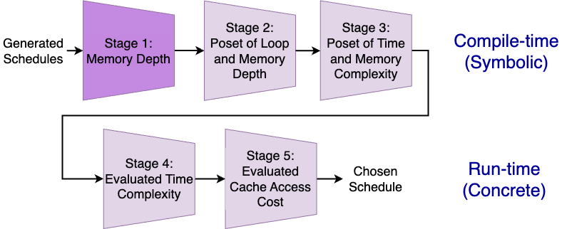
Figure 6. Pruning Stages of the auto-scheduler. The light purple stages compare one schedule against other schedules for pruning. The dark purple stage uses an absolute measure for pruning without comparing it against other schedules. The top 3 stages in the diagram are executed during the compile-time with symbolic expressions in stages 2 and 3. The bottom 2 stages in the diagram are executed at run-time after evaluating symbolic expressions with real values.

5.1. Schedule Generation

For a given expression and an LIG, we generate all the loop index orders that conform to the sparse tensor constraints (i.e. that do not violate sparse index access patterns in the sparse tensors). Then we split the input tensors in the tensor contraction at different positions for all those index orders. For example, the input tensors in Figure 3 can be split at any position in $IT_{1}$ to $IT_{E}$. Once input tensors in the tensor contraction are split at different positions, we infer the temporary indices and call the same function recursively for both the consumer and producer sub-computations. Once those sub-computations return the consumer schedules $C_{Schedules}$ and producer schedules $P_{Schedules}$, we combine those 2 schedule spaces $P_{Schedules}\times C_{Schedules}$ to create super schedules that completely describe the required initial computation. If the producer and consumer sections can be fused as mentioned in Section 4.2, we merge the sub-computations to create fused schedules which are then added to the list of schedules. We use caching to help reduce the schedule generation time.

5.2. Memory Depth Based Pruning

The first pruning stage uses the dimensionality of the temporary tensors used in the computation. For example, Schedule 1(a) does not use any intermediate temporaries. Hence, the memory depth is $0$. In Schedule 1(b), $T<K>$ relates to a memory depth of just $1$ whereas Schedules 1(c)- 1(d) all have a memory depth of $2$ since 2D temporary tensors are used in the computation. In our example, if the fusion did not happen and we split the computation to $T_{jkl}=B_{ijk}*C_{jl}$ and $A_{lmn}=T_{jkl}*D_{jm}*E_{kn}$, the memory depth would be $3$, and this extra temporary would likely consume a lot of memory. A greater memory depth increases the likelihood for a given computation to consume more memory due to memory depth being multiplicative. As such, we use this heuristic to prune the schedules that have a memory depth greater than or equal to $3$.

We chose this heuristic for the first stage because it helps prune a large number of schedules that are likely to consume a large amount of memory leading to slow execution times. At the end of this stage, we compute the symbolic iteration time complexity and symbolic auxiliary memory complexity of each of the schedules and allocate them into baskets (same set) if they have the same complexities.

5.3. Loop and Memory Depth Based Pruning

In Section 3, we explained how using only the loop depth at a time could prune potentially useful schedules. Therefore, at this stage, we consider both the loop depth and memory depth for pruning. We use a partially ordered set (poset) based pruning mechanism to prune the schedules that are worse in terms of both loop depth and memory depth compared to another schedule. We call this poset-based pruning because, in this stage, we create partially ordered sets of schedules based on the loop depth and memory depth of the schedules and select the schedules that are not dominated by any other schedule considering both criteria. This poset-based pruning mechanism ensures that fused schedules contain all the schedules with simple linear loop nests with no branches, including the default fully fused schedule by TACO. This guarantees that we end up with a superior schedule in the end compared to the default schedule. The memory depth heuristic we used in Stage 1 in Section 5.2 ensures that we do not prune schedules that are likely to have lesser loop depth than the fused simple linear loop nest schedules without branches. The poset-based pruning mechanism can be formally written as follows.

This stage removes $s^{\prime}$ from the set of schedules $S$ from Stage 1 if $\exists$ $c^{\prime}\in S$ s.t.

$$(L(s^{\prime})>L(c^{\prime})\land M(s^{\prime})>=M(c^{\prime}))\lor(L(s^{\prime})>=L(c^{\prime})\land M(s^{\prime})>M(c^{\prime}))$$

where $L(s^{\prime})$ and $M(s^{\prime})$ are the loop depth and memory depth of the schedule $s^{\prime}$ respectively. This prune schedules that are worse in terms of both loop depth and memory depth compared to another schedule. This kind of Poset-based pruning is important to ensure that we do not remove schedules that are likely to be better.

5.4. SMT Solver Based Pruning

In some cases, the user (eg: performance engineer) may know some information about the loop bounds or sparsities of the sparse tensors used in the computation during the compile time. For example, if it is a graph neural network computation, the user may know that the feature size of the nodes is only going to change between 16 and 256, or the user may know that the graph size is on the order of 10 million and the sparsity of the graph is going to fall somewhere between 0.01 and 0.001. Then, the user can provide those values as a range and the auto-scheduler can use an SMT solver to reason about the time and memory complexities of the schedules using symbolic cost expressions that it builds for each schedule as explained in Section 3. Note that in this kind of reasoning, we have to assume that the tensors have uniform sparsities. There are 3 types of constraints that we can inject into the SMT solver; (1) Range constraints: the range in which dense loop bounds and sparsities can vary; (2) Inferred constraints: non-zero values in a sparse tensor are always less than the number of non-zero values in its dense representation and the non-affine loop that iterates through the sparse tensor will vary between 0 and the dense loop bound that defines the sparse tensor; (3) User-defined constraints: other special constraints that the user may know about the loop bounds or sparsities. For example, the user may know that the sparsity is equal to the square root of some dense loop bound, or that one loop bound is twice another.

After injecting the constraints known at compile time to the environment, we check if one schedule is dominated by at least one other schedule in the schedule space in terms of both iteration time and auxiliary memory complexities, then we remove that schedule from the Pareto frontier. This procedure can be formally written as follows.

Let user-defined constraints of loop bounds and sparsities be $\Phi$, let $Z3$ be the SMT solver, and the schedules from Stage 2 be $S$. Inject $\Phi$ into $Z3$.
Remove $s^{\prime}$ from $S$ if $\exists$ $c^{\prime}\in S$ s.t.
$\exists$ loop bounds and sparsities s.t.

$$(T(s^{\prime})>T(c^{\prime})\land N(s^{\prime})>=N(c^{\prime}))\lor(T(s^{\prime})>=T(c^{\prime})\land N(s^{\prime})>N(c^{\prime}))$$

$\nexists$ loop bounds and sparsities s.t.

$$(T(s^{\prime})<=T(c^{\prime})\land N(s^{\prime})<N(c^{\prime}))\lor(T(s^{\prime})<T(c^{\prime})\land N(s^{\prime})<=N(c^{\prime}))$$

Here, $T(s^{\prime})$ and $N(s^{\prime})$ denote the symbolic iteration time complexity and symbolic additional memory complexity of the schedule $s^{\prime}$ respectively.

An auto-scheduler could have this stage alone without the previous stage in Section 5.3. But, when any of the above conditions are $unsat$, the $Z3$ SMT solver takes a long time to complete the computation and return. The previous stage compares a lot more schedules than this stage. Therefore, using a comparative (i.e. absolute values of depth for comparison) poset-based pruning strategy, which is lighter in terms of computing, is beneficial compared to using an SMT solver. Nonetheless, this stage is important because we can further reduce the number of schedules evaluated at run time with the information available to the user at compile time by using an SMT solver.

5.5. Time Complexity Based Pruning

This is the first stage of filtration at runtime. We evaluate the symbolic iteration time complexity and auxiliary memory complexity expressions with real values available at runtime and select the schedules that have the least iteration time complexity such that the auxiliary memory complexity is less than 50% of the last level cache (LLC) from the Pareto frontier. We take 50% as a rough margin for the selection criterion on the assumption that there is 50% of LLC available for the other input and output tensors in the computation. There can be multiple schedules with the same iteration time complexity due to having the same branched loop nest structure with different loop reorderings. These schedules are then passed to the next stage for further pruning.

5.6. Cache Based Pruning

We now consider the second runtime-based pruning method, cache-based pruning. The cache-based pruning stage is not a focus of this paper and we have it in place for completeness. Of the remaining schedules, many of them could have equivalent time and memory complexity due to loop reorderings. For example, both the loop orders $l,m$, and $m,l$ in the outer loop of Figure 1(b) have the same time and auxiliary memory complexities.

Since both schedules will have the same time and memory complexity, if one of these schedules was unpruned by previous methods, they both would remain unpruned. Thus, we have a simple model that assigns a cache access cost to each of the models. This cache model takes 2 criteria into account. (1) it looks at the leaves in the BIG and the leaf loop index. If the leaf loop index is $i$ and if a tensor in the compute expression at that leaf branch has $i$ as the last index (eg: $B(j,i)$) or index $i$ is not present in the tensor (eg: $B(j,k)$), then the cost of access is zero. If $i$ is present and not in the last accessed index (eg: $B(i,j)$), then we take the cache access cost as $j$ since elements are accessed $J$ locations apart. We assign costs to all the leaves in the BIG and sum those to calculate a final cache access cost. We take the last index of the leaves in the BIG into consideration because it has the highest impact in terms of both temporal and spatial cache locality. (2) We give precedence to the schedules that have the same index order as the loop order in the iteration graph. For example, if tensors in the computation have $B(i,j)$ and $C(j,k)$, it would favor the loop order $i,j,k$ over $k,j,i$. If both these criteria are the same in 2 schedules, we randomly select one of them.

6. Evaluation

Kernel	Description	Chosen Schedules After Z3 Pruning
$\langle SDDMM,SpMM\rangle$	$A_{il}=\displaystyle\sum_{jk}{{\textbf{{B}}}_{ij}}\>C_{ik}\>D_{jk}\>E_{jl}$	$i,{{\textbf{{j}}}^{\prime}}\left\langle t;k:t+={{\textbf{{B}}}_{ij}}\>C_{ik}\>D_{jk},l:A_{il}+=t\>E_{jl}\right\rangle$
$\langle SDDMM,SpMM,GEMM\rangle$	$A_{im}=\displaystyle\sum_{jkl}{{\textbf{{B}}}_{ij}}\>C_{ik}\>D_{jk}\>E_{jl}\>F_{lm}$	$i\left\langle T_{l};\right.$ $\enspace{{\textbf{{j}}}^{\prime}}\left\langle t;k:t+={{\textbf{{B}}}_{ij}}\>C_{ik}\>D_{jk},l:T_{l}^{1}+=t\>E_{jl}\right\rangle,$ $\enspace\left.m,l:A_{im}+=T_{l}\>F_{lm}\right\rangle$
		$i,{{\textbf{{j}}}^{\prime}}\left\langle t;k:t+={{\textbf{{B}}}_{ij}}\>C_{ik}\>D_{jk},m,l:A_{il}+=t\>E_{jl}\>F_{lm}\right\rangle$
		$i,l\left\langle t;{{\textbf{{j}}}^{\prime}},k:t+={{\textbf{{B}}}_{ij}}\>C_{ik}\>D_{jk}\>E_{jl},m,l:A_{il}+=t\>F_{lm}\right\rangle$
$\langle SpMMH,GEMM\rangle$	$A_{il}=\displaystyle\sum_{jk}{{\textbf{{B}}}_{ij}}\>C_{jk}\>D_{jk}\>E_{kl}$	$i,{{\textbf{{j}}}^{\prime}}\left\langle t;k:t+={{\textbf{{B}}}_{ij}}\>C_{jk}\>D_{jk},l:A_{il}+=t\>E_{jl}\right\rangle$
$\langle SpGEMM,GEMM\rangle$	$A_{il}=\displaystyle\sum_{jk}{{\textbf{{B}}}_{ij}}\>C_{jk}\>D_{kl}$	$i,k\left\langle t;{{\textbf{{j}}}^{\prime}}:t+={{\textbf{{B}}}_{ij}}\>C_{jk}\>,l:A_{il}+=t\>D_{kl}\right\rangle$
$\langle 3D\ TTMC\rangle$	$A_{lmn}=\displaystyle\sum_{ijk}{{\textbf{{B}}}_{ijk}}\>C_{il}\>D_{jm}\>E_{kn}$	$i,{{\textbf{{j}}}^{\prime}},n\left\langle t;{{\textbf{{k}}}^{\prime}}:t+={{\textbf{{B}}}_{ijk}}\>E_{kn}\>,m,l:A_{lmn}+=t\>C_{il}\>D_{jm}\right\rangle$
		$i,n\left\langle T_{m};\right.$ $\enspace{{\textbf{{j}}}^{\prime}}\left\langle t;{{\textbf{{k}}}^{\prime}}:t+={{\textbf{{B}}}_{ijk}}\>E_{kn},m:T_{m}+=t\>D_{jm}\right\rangle,$ $\enspace\left.m,l:A_{lmn}+=T_{m}\>C_{il}\right\rangle$
		$i,m,n\left\langle t;{{\textbf{{j}}}^{\prime}},{{\textbf{{k}}}^{\prime}}:t+={{\textbf{{B}}}_{ijk}}\>D_{jm}\>E_{kn}\>,m,l:A_{lmn}+=t\>C_{il}\right\rangle$
$\langle SpTTM,TTM\rangle$	$A_{ilm}=\displaystyle\sum_{jk}{{\textbf{{B}}}_{ijk}}\>C_{jl}\>D_{km}$	$i{{\textbf{{j}}}^{\prime}}m{{\textbf{{k}}}^{\prime}}l:A_{ilm}+=B_{ijk}\>C_{jl}\>D_{km}$
		$i,{{\textbf{{j}}}^{\prime}}m\left\langle t;{{\textbf{{k}}}^{\prime}}:t+={{\textbf{{B}}}_{ijk}}\>D_{jk},l:A_{il}+=t\>C_{jl}\right\rangle$
$\langle SpTTM,SpTTM\rangle$	${{\textbf{{A}}}_{ijm}}=\displaystyle\sum_{jk}{{\textbf{{B}}}_{ijk}}\>C_{kl}\>D_{lm}$	$i,{{\textbf{{j}}}^{\prime}}l\left\langle t;{{\textbf{{k}}}^{\prime}}:t+={{\textbf{{B}}}_{ijk}}\>C_{kl},m:{{\textbf{{A}}}_{il}}+=t\>D_{lm}\right\rangle$
$\langle MTTKRP,GEMM\rangle$	$A_{im}=\displaystyle\sum_{jk}{{\textbf{{B}}}_{ikl}}\>C_{lj}\>D_{kj}\>E_{jm}$	$i,{{\textbf{{j}}}^{\prime}}\left\langle t;{{\textbf{{k}}}^{\prime}}l:t+={{\textbf{{B}}}_{ijk}}\>C_{kl}\>D_{kj},m:A_{il}+=t\>E_{jm}\right\rangle$

Figure 7. The figure includes the descriptions, names of the kernels used in the evaluation, and the final schedules chosen by the auto-scheduler after the SMT solver-based pruning stage. The tensors or matrices in boldface capital letters denote sparse tensors or matrices. The boldface small letters with an apostrophe denote the corresponding non-affine loops of the indices in the computation in the description. Different kernels inside the angle brackets denote that the fused computation can be separated into those kernels. The inner branches of the loop nests are written as $\left\langle Temporary;Producer,Consumer\right\rangle$ under the Chosen Schedules column.

Kernel	Generated Schedules	Stage 1 Mem Depth	Stage 2 Depth Poset	Stage 3 SMT Solver
$\langle SDDMM,SpMM\rangle$	$16\,169$	$1472$ (255)	1 (1)	1 (1)
			-	1 (1)
$\langle SDDMM,SpMM,GEMM\rangle$	$145\,448\,232$	$207\,129$ ($18\,277$)	224 (43)	8 (3)
			-	32 (4)
$\langle SpMMH,GEMM\rangle$	$7426$	692 (133)	2 (1)	2 (1)
			-	2 (1)
$\langle SpGEMM,GEMM\rangle$	258	128 (34)	2 (1)	2 (1)
			-	2 (1)
$\langle 3D\ TTMC\rangle$	$14\,701\,776$	$30\,203$ ($2541$)	101 (26)	16 (3)
			-	16 (3)
$\langle SpTTM,TTM\rangle$	$2561$	352 (60)	3 (1)	3 (1)
			-	3 (1)
$\langle SpTTM,SpTTM\rangle$	109	46 (13)	1 (1)	1 (1)
			-	1 (1)
$\langle MTTKRP,GEMM\rangle$	$58\,127$	$4715$ (728)	5 (2)	2 (1)
			-	2 (1)

Figure 8. The number of schedules after each stage in the pruning pipeline. The numbers in the parenthesis denote the number of different (time complexity, auxiliary memory complexity) pairs. We allocate each schedule to a different (time, memory) bucket. In other words, the schedules in a bucket have the same iteration time and memory complexities but their loop orders are different. We report the number of schedules when we bypass Stage 2 and directly send Stage 1 schedules to Stage 3 to see if we get a different set of schedules without Stage 2, in the $2^{nd}$ row in the last column of each kernel. We see the same results as before for most of the kernels.

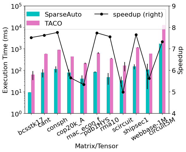
(a) ${\langle{SDDMM,SpMM}\rangle}$

[sddmm-spmm evaluation graph]¡long description¿

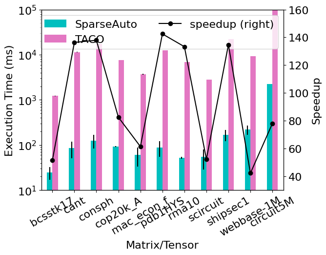
(b) ${\langle{SDDMM,SpMM,GEMM}\rangle}$

[sddmm-spmm-gemm evaluation graph]¡long description¿

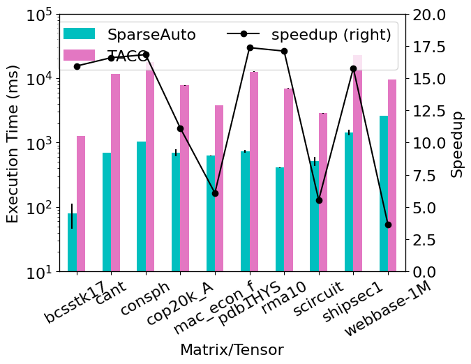
(c) ${\langle{SpMMH,GEMM}\rangle}$

[spmmh-gemm evaluation graph]¡long description¿

(d) ${\langle{SpGEMM,GEMM}\rangle}$

[spmm-gemm evaluation graph]¡long description¿

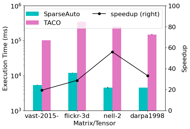
(e) ${\langle{3D\ TTMC}\rangle}$

[3D tensor contraction evaluation graph]¡long description¿

(f) ${\langle{SpTTM,TTM}\rangle}$

[spttm-ttm evaluation graph]¡long description¿

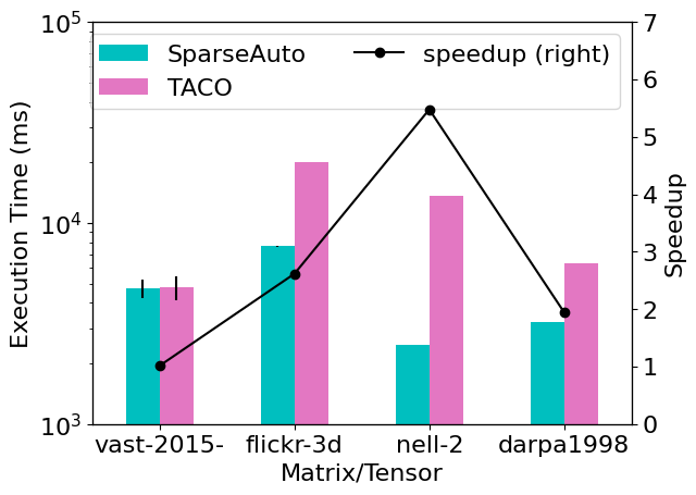
(g) ${\langle{SpTTM,SpTTM}\rangle}$

[spttm-spttm evaluation graph]¡long description¿

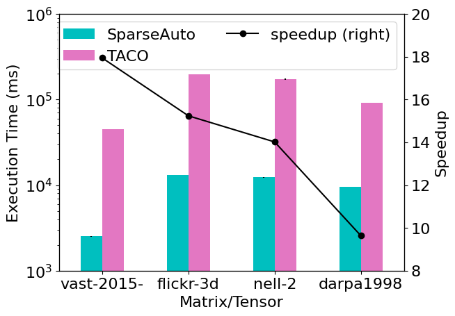
(h) ${\langle{MTTKRP,GEMM}\rangle}$

[mttkrp-gemm evaluation graph]¡long description¿

Figure 9. Performance Comparison with TACO.

We evaluate our approach on a set of sparse tensor kernels against the TACO (Kjolstad et al., 2017a) generated schedule.

6.1. Experimental Setup

We run the experiments on an Intel(R) Xeon(R) CPU E5-4650 32-core processor at 2.70 GHz with 32KB L1 data cache, 256KB L2 cache, and 20MB LLC shared per 4 cores. We compile the code using GCC 11.4.0 with -O3 –ffast-math. All experiments are run on a single core except for schedule generation. We execute a warm-up run and then execute the kernel computation 31 times and report the median with the corresponding standard deviation for the 31 runs. We use many real-world matrices and tensors described in Section 6.2 in the evaluation.

6.2. Datasets

The sparse matrices and tensors used in the evaluation are obtained from the SuiteSparse Collection (Davis and Hu, 2011), Network Repository (Rossi et al., 2015), Formidable Repository of Open Sparse Tensors and Tools (Smith et al., 2017), and 1998 DARPA Intrusion Detection Evaluation Dataset (Cunningham et al., 2000). The details of the datasets are shown in Table 1.

Table 1. Test tensors used in the evaluation from various matrix and tensor collections mentioned in the Section 6.2

Tensor Dimensions Non-zeros Sparsity bcsstk17 $11K\times 11K$ $429K$ 4E-3 pdb1HYS $36K\times 36K$ $4.34M$ 3E-3 rma10 $47K\times 47K$ $2.37M$ 1E-3 cant $62K\times 62K$ $4.01M$ 1E-3 consph $83K\times 83K$ $6.01M$ 9E-4 cop20k_A $12K\times 12K$ $2.62M$ 2E-4 shipsec1 $140K\times 140K$ $7.81M$ 2E-4 scircuit $171K\times 171K$ $959K$ 3E-5 mac_econ_fwd500 $207K\times 207K$ $1.27M$ 9E-5 webbase-1M $1.00M\times 1.00M$ $3.11M$ 3E-6 circuit5M $5.56M\times 5.56M$ $59.52M$ 2E-6 flickr-3d $320K\times 2.82M\times 1.60M$ $112.89M$ 3.92E-11 nell-2 $12K\times 9K\times 288K$ $76.88M$ 5.73E-05 vast-2015-mc1-3d $165K\times 11K\times 2$ $26.02M$ 8.36E-08 darpa1998 $22K\times 22K\times 23.7M$ $28.42M$ 2.50E-06

6.3. Kernels

We evaluate the performance of the kernel shown in Figure 7. We compare our approach with TACO (Kjolstad et al., 2017a). $SDDMM$ Sampled Dense-Dense Matrix Multiplication and $SpMM$ Sparse Matrix-Matrix multiplication are used in graph neural networks. $\langle 3DSpTTMC\rangle$ Tensor-Times Matrix Contractions are used in Tucker Decompositions (Tucker, 1966). We use combinations of these kernels in the evaluation. Note that the naming conventions for the superscript are as follows: $\langle SDDMM,\allowbreak SpMM\rangle$ means that the kernel is a combination of $SDDMM$ and $SpMM$ and the kernel can be separated to those two sub-kernels that can be performed one after the other. Figure 9 shows the execution times and speedups of the selected schedules against the default TACO schedule. We observe orders of magnitude better performance compared to TACO. We notice that the schedule selected by the auto-scheduler for the schedules $\langle SDDMM,\allowbreak SpMM\rangle$, $\langle SDDMM,\allowbreak SpMM,\allowbreak GEMM\rangle$, $\langle SpMMH,\allowbreak GEMM\rangle$, $\langle SpGEMM,GEMM\rangle$, and $\langle MTTKRP,\allowbreak GEMM\rangle$ are same as that of the schedules reported by in the SparseLNR (Dias et al., 2022).

Ahrens et al. (Ahrens et al., 2022) uses a different version of the
${\langle{SpGEMM,GEMM}\rangle}$ kernel where $D$ is transposed – $A_{il}=\sum_{jk}{{\textbf{{B}}}_{ij}}\>C_{jk}\>D_{lk}$. SparseLNR (Dias et al., 2022) uses the same kernel format as ours. The selected kernel of both those works is $i\langle T_{k}{,}$$\ {{\textbf{{j}}}^{\prime}}k:T_{k}+={{\textbf{{B}}}_{ij}}\>C_{jk}\>{,}$$\ lk:A_{il}+=T_{k}\>D_{lk}\rangle$ with an extra 1D auxiliary memory. The schedule picked by our auto-scheduler dominates this schedule in terms of auxiliary memory because the schedule in Figure 7 uses a scalar memory. The schedule with 1D auxiliary memory works better than ours for $A_{il}=\sum_{jk}{{\textbf{{B}}}_{ij}}\>C_{jk}\>D_{lk}$ and $A_{il}=\sum_{jk}{{\textbf{{B}}}_{ij}}\>C_{jk}\>D_{kl}$. But the schedule with the scalar auxiliary memory outperforms the one with 1D auxiliary memory for $A_{il}=\sum_{jk}{{\textbf{{B}}}_{ij}}\>C_{kj}\>D_{kl}$ and $A_{il}=\sum_{jk}{{\textbf{{B}}}_{ij}}\>C_{kj}\>D_{lk}$ versions. One schedule performs better in one instance and not in the other because of the cache access effects when the transpose of the matrices is used. To avoid this, the auto-scheduler would be required to reason about the cache misses and the cache access patterns. This is beyond the scope of this paper. We leave this as future work.

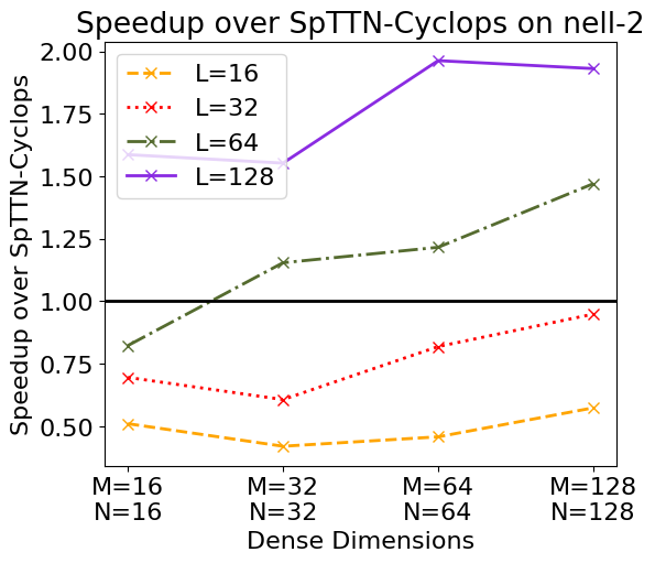
(a)   

[Comparison of TTMC with SpTTN-Cyclops for nell-2 dataset]¡long description¿

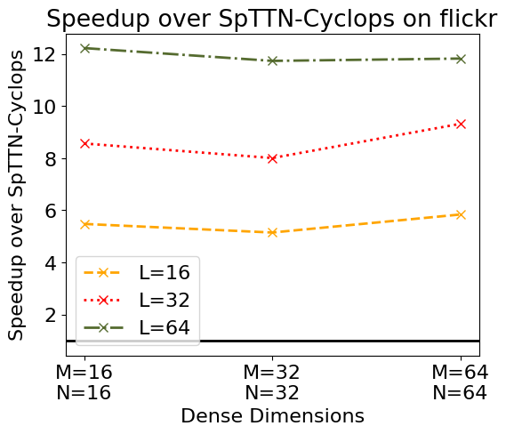
(b)   

[comparison of TTMC with SpTTN-Cyclops with flickr datataset]¡long description¿

Figure 10. Performance Comparison with SpTTN-Cyclops of $TTMC$ kernel by varying dense dimensions $L$, $M$, and $N$.

We compare our selected schedule with the SpTTN-Cyclops (Kanakagari and Solomonik, 2023) selected schedule for $3D\ TTMC$ kernel for $flickr$ and $nell-2$ datasets (See Figure 10). Since their auto-scheduler does not optimize for memory, their schedule is $i\langle T_{mn}^{2};$$\>{{\textbf{{j}}}^{\prime}}\langle T_{n}^{1};{{\textbf{{k}}}^{\prime}},n:T_{n}^{1}+={{\textbf{{B}}}_{ijk}}\>E_{kn},m,n:T_{mn}^{2}+=T_{n}^{1}\>D_{jm}\rangle;$$\>l,m,n:A_{lmn}+=T_{mn}^{2}\>C_{il}\rangle$ with one 2D and another 1D intermediate temporaries whereas our schedule $i,n\langle T_{m};$$\>{{\textbf{{j}}}^{\prime}}\langle t;{{\textbf{{k}}}^{\prime}}:t+={{\textbf{{B}}}_{ijk}}\>E_{kn},m:T_{m}+=t\>D_{jm}\rangle;$$\>m,l:A_{lmn}+=T_{m}\>C_{il}\rangle$ uses only one scalar and one 1D intermediate temporaries. When the temporary sizes as dictated by M and N dimensions are large and the temporaries are accessed more frequently as dictated by L, our schedule tends to perform better. For smaller temporaries and fewer temporary access frequencies, SpTTN-Cyclops (Kanakagari and Solomonik, 2023) tends to perform better. Note that both these schedules have the same iteration time complexity. The speedup differences stem from cache accesses. SpTTN-Cyclops maps computations to BLAS calls. We omitted this mapping of BLAS calls in our evaluation.

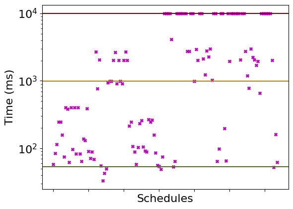
(a)   

[bcsstk17 for all schedules with K,L dense dimensions set to 64]¡long description¿

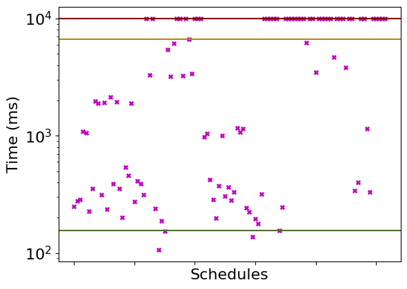
(b)   

[bcsstk17 for all schedules with K,L dense dimensions set to 128]¡long description¿

Figure 11. Performance Comparison of SparseAuto with all of the other schedules for $\langle SpMM,GEMM\rangle$ kernel with dense dimensions $K$, $L$ set to 64 (left) and 128 (right). The green line corresponds to the execution time of SparseAuto, the gold line corresponds to the execution time of the default TACO schedule, and the red line represents the timeout of the evaluation.

Furthermore, we compare the performance of SparseAuto selected schedule with all of the other schedules in Figure 11 for a kernel with a fewer number of schedules. We see that SparseAuto selected schedule is at the top few best schedules.

7. Related Works

There have been several works on dense and sparse tensor contractions relating to tensor compilers, compiler optimizations, and targeted optimizations for specific kernels.

Loop optimizations for dense tensor algebra have been extensively studied in the literature for decades. The research works (Sahoo et al., 2005; Allam et al., 2006; Sahoo et al., 2005; Cociorva et al., 2003) focus on CPU optimizations for dense tensor contractions targetting memory-constrained environments. Dense transformations are relatively easier compared to sparse transformations and scheduling because array accesses are not constrained by the structure or sparse access patterns in dense tensors or arrays. The research works (Nelson et al., 2015a; Kim et al., 2019; Abdelfattah et al., 2016; Nelson et al., 2015b) focus on GPU optimizations for dense tensor computations. However, they are not applicable to sparse tensor computations because sparse tensors do not have random access and the intricacies of sparse data structures and non-affine loops in the computations.

The Tensor Contraction Engine (TCE)  (Auer et al., 2006) generates code targetting a given amount of main memory and uses a feedback loop to a memory minimization module to fuse more loops to reduce auxiliary memory usage. Their approach is for dense tensor computations and differs from our approach which uses a poset-based mechanism. The research works (Lam et al., 1997; Hartono et al., 2009) works along similar optimization as TCE for dense tensors. Johnnie et al.  (Gray and Kourtis, 2021) maps the tensor contraction problem to a graph problem focusing on dense tensor contractions.

General sparse tensor algebra compilers such as TACO (Kjolstad et al., 2017a), COMET (Tian et al., 2021b), Sparsifier (Bik et al., 2022) in MLIR focus on generating general code for sparse tensor computations but they cannot generate nested multiple levels of loop branches and they do not have a mechanism to explore the search space. SparseTIR (Ye et al., 2023), SparseLNR (Dias et al., 2022), and ReACT (Zhou et al., 2023) can generate fused sparse loops but they are limited, and not versatile enough to let the user generate arbitrary loop nests with multiple branches and explore the search space.

Ahrens et al.  (Ahrens et al., 2022) introduces an auto-scheduler that focuses on loop depth and then later uses an asymptotic cost model to prune the search space. They do not optimize for both time and auxiliary memory complexities. Their auto-scheduler is completely offline and does not use user-defined constraints at compile time to prune the search space. Their system has the disadvantages described in detail in Section 3. Their framework evaluated on TACO cannot support intermediate temporaries with more than 1 dimension. They focus on data layout transformations in their auto-scheduler.

Kanakagari et al.  (Kanakagari and Solomonik, 2023) is another auto-scheduler for sparse tensor contractions. Their framework is a complete auto-scheduler and the user has no control over selecting their schedule with manual scheduling directives. They do not focus on posed-based pruning, instead, they also select the minimum loop depth schedules, which may not be optimal as we explained in Section 3. They do not support the use of user-defined constraints on an SMT solver to reason about the complexities of the schedules to prune the search space. Their loop generation algorithm runs at runtime with effects on the evaluation time whereas our method minimizes the number of schedules evaluated at runtime. They limit their code generation to 1 sparse input tensor and if the output tensor is sparse, then it needs to have the same sparsity structure as the input sparse tensor in the tensor contraction. Our scheduling primitive is more general.

References

• (1)
• Abdelfattah et al. (2016) A. Abdelfattah, M. Baboulin, V. Dobrev, J. Dongarra, C. Earl, J. Falcou, A. Haidar, I. Karlin, Tz. Kolev, I. Masliah, and S. Tomov. 2016. High-performance Tensor Contractions for GPUs. Procedia Computer Science 80 (2016), 108–118. https://doi.org/10.1016/j.procs.2016.05.302 International Conference on Computational Science 2016, ICCS 2016, 6-8 June 2016, San Diego, California, USA.
• Ahrens et al. (2022) Willow Ahrens, Fredrik Kjolstad, and Saman Amarasinghe. 2022. Autoscheduling for Sparse Tensor Algebra with an Asymptotic Cost Model. In Proceedings of the 43rd ACM SIGPLAN International Conference on Programming Language Design and Implementation (San Diego, CA, USA) (PLDI 2022). Association for Computing Machinery, New York, NY, USA, 269–285. https://doi.org/10.1145/3519939.3523442
• Allam et al. (2006) A. Allam, J. Ramanujam, G. Baumgartner, and P. Sadayappan. 2006. Memory minimization for tensor contractions using integer linear programming. In Proceedings 20th IEEE International Parallel Distributed Processing Symposium. 8 pp.–. https://doi.org/10.1109/IPDPS.2006.1639717
• Auer et al. (2006) Alexander A. Auer, Gerald Baumgartner, David E. Bernholdt, Alina Bibireata, Daniel Cociorva Venkatesh Choppella, Xiaoyang Gao, Robert Harrison, Sandhya Krishnan Sriram Krishnamoorthy, Chi-Chung Lam, Qingda Lu, Marcel Nooijen, Russell Pitzer, J. Ramanujam, P. Sadayappan, and Alexander Sibiryakov. 2006. Automatic code generation for many-body electronic structure methods: the tensor contraction engine. Molecular Physics 104, 2 (2006), 211–228. https://doi.org/10.1080/00268970500275780 arXiv:https://doi.org/10.1080/00268970500275780
• Bik et al. (2022) Aart Bik, Penporn Koanantakool, Tatiana Shpeisman, Nicolas Vasilache, Bixia Zheng, and Fredrik Kjolstad. 2022. Compiler Support for Sparse Tensor Computations in MLIR. ACM Trans. Archit. Code Optim. 19, 4, Article 50 (sep 2022), 25 pages. https://doi.org/10.1145/3544559
• Bik and Wijshoff (1993) Aart J. C. Bik and Harry A. G. Wijshoff. 1993. Compilation Techniques for Sparse Matrix Computations. In Proceedings of the 7th International Conference on Supercomputing (Tokyo, Japan) (ICS ’93). Association for Computing Machinery, New York, NY, USA, 416–424. https://doi.org/10.1145/165939.166023
• Chou et al. (2018) Stephen Chou, Fredrik Kjolstad, and Saman Amarasinghe. 2018. Format Abstraction for Sparse Tensor Algebra Compilers. Proc. ACM Program. Lang. 2, OOPSLA, Article 123 (oct 2018), 30 pages. https://doi.org/10.1145/3276493
• Cociorva et al. (2003) D. Cociorva, Xiaoyang Gao, S. Krishnan, G. Baumgartner, Chi-Chung Lam, P. Sadayappan, and J. Ramanujam. 2003. Global communication optimization for tensor contraction expressions under memory constraints. In Proceedings International Parallel and Distributed Processing Symposium. 8 pp.–. https://doi.org/10.1109/IPDPS.2003.1213121
• Cunningham et al. (2000) R. K. Cunningham, R. P. Lippmann, D. J. Fried, S. L. Garfinkel, I. Graf, K. R. Kendall, S. E. Webster, D. Wychogrod, and M. A. Zissman. 2000. Evaluating Intrusion Detection Systems without Attacking your Friends: The 1998 DARPA Intrusion Detection Evaluation. Proceedings of the 2000 DARPA Information Survivability Conference and Exposition (DISCEX’00) (2000), 12–26. https://doi.org/10.1109/DISCEX.2000.823339
• Davis and Hu (2011) Timothy A. Davis and Yifan Hu. 2011. The University of Florida Sparse Matrix Collection. ACM Trans. Math. Softw. 38, 1, Article 1 (dec 2011), 25 pages. https://doi.org/10.1145/2049662.2049663
• Dias et al. (2022) Adhitha Dias, Kirshanthan Sundararajah, Charitha Saumya, and Milind Kulkarni. 2022. SparseLNR: accelerating sparse tensor computations using loop nest restructuring. In Proceedings of the 36th ACM International Conference on Supercomputing.
• Gray and Kourtis (2021) Johnnie Gray and Stefanos Kourtis. 2021. Hyper-optimized tensor network contraction. Quantum 5 (March 2021), 410. https://doi.org/10.22331/q-2021-03-15-410
• Hamilton et al. (2017) Will Hamilton, Rex Ying, and Jure Leskovec. 2017. Inductive representation learning on large graphs. Advances in neural information processing systems 30 (2017), 1024–1034.
• Hartono et al. (2009) Albert Hartono, Qingda Lu, Thomas Henretty, Sriram Krishnamoorthy, Huaijian Zhang, Gerald Baumgartner, David E. Bernholdt, Marcel Nooijen, Russell Pitzer, J. Ramanujam, and P. Sadayappan. 2009. Performance Optimization of Tensor Contraction Expressions for Many-Body Methods in Quantum Chemistry. The Journal of Physical Chemistry A 113, 45 (2009), 12715–12723. https://doi.org/10.1021/jp9051215 arXiv:https://doi.org/10.1021/jp9051215 PMID: 19888780.
• Hirato ([n. d.]) So Hirato. [n. d.]. Tensor Contraction Engine: Abstraction an Automated Parallel Implementation of Configuration-Interaction, Coupled-Cluster, and Many-Body Perturbation Theories. The journal of physical chemistry. A 107, 46 ([n. d.]), 9887–9897. https://doi.org/10.1021/jp034596z
• Hu et al. (2020) Yuwei Hu, Zihao Ye, Minjie Wang, Jiali Yu, Da Zheng, Mu Li, Zheng Zhang, Zhiru Zhang, and Yida Wang. 2020. FeatGraph: A Flexible and Efficient Backend for Graph Neural Network Systems. In Proceedings of the International Conference for High Performance Computing, Networking, Storage and Analysis (Atlanta, Georgia) (SC ’20). IEEE Press, Article 71, 13 pages.
• Kanakagari and Solomonik (2023) Raghavendra Kanakagari and Edgar Solomonik. 2023. Minimum Cost Loop Nests for Contraction of a Sparse Tensor with a Tensor Network. https://doi.org/10.48550/arXiv.2307.05740
• Kim et al. (2019) Jinsung Kim, Aravind Sukumaran-Rajam, Vineeth Thumma, Sriram Krishnamoorthy, Ajay Panyala, Louis-Noël Pouchet, Atanas Rountev, and P. Sadayappan. 2019. A Code Generator for High-Performance Tensor Contractions on GPUs. In 2019 IEEE/ACM International Symposium on Code Generation and Optimization (CGO). 85–95. https://doi.org/10.1109/CGO.2019.8661182
• Kjolstad et al. (2019) Fredrik Kjolstad, Peter Ahrens, Shoaib Kamil, and Saman Amarasinghe. 2019. Tensor Algebra Compilation with Workspaces. none 0 (2019), 180–192. http://dl.acm.org/citation.cfm?id=3314872.3314894
• Kjolstad et al. (2017a) Fredrik Kjolstad, Shoaib Kamil, Stephen Chou, David Lugato, and Saman Amarasinghe. 2017a. The Tensor Algebra Compiler. Proc. ACM Program. Lang. 1, OOPSLA, Article 77 (Oct. 2017), 29 pages. https://doi.org/10.1145/3133901
• Kjolstad et al. (2017b) Fredrik Kjolstad, Shoaib Kamil, Stephen Chou, David Lugato, and Saman Amarasinghe. 2017b. The Tensor Algebra Compiler. Proc. ACM Program. Lang. 1, OOPSLA, Article 77 (Oct. 2017), 29 pages. https://doi.org/10.1145/3133901
• Kossaifi et al. (2017) Jean Kossaifi, Aran Khanna, Zachary Lipton, Tommaso Furlanello, and Anima Anandkumar. 2017. Tensor Contraction Layers for Parsimonious Deep Nets. In Proceedings of the IEEE Conference on Computer Vision and Pattern Recognition (CVPR) Workshops.
• Kotlyar et al. (1997) Vladimir Kotlyar, Keshav Pingali, and Paul Stodghill. 1997. A Relational Approach to the Compilation of Sparse Matrix Programs. In Proceedings of the Third International Euro-Par Conference on Parallel Processing (Euro-Par ’97). Springer-Verlag, Berlin, Heidelberg, 318–327.
• Lam et al. (1997) Chi-Chung Lam, P. Sadayappan, and Rephael Wenger. 1997. On Optimizing a Class of Multi-Dimensional Loops with Reductions for Parallel Execution. Parallel Process. Lett. 7 (1997), 157–168. https://api.semanticscholar.org/CorpusID:9440379
• Markov (2008) Igor L. an Shi Yaoyun Markov. 2008. Simulating Quantum Computation by Contracting Tensor Networks. SIAM J. Comput. 38, 3 (2008), 963–981. https://doi.org/10.1137/050644756
• Nelson et al. (2015a) Thomas Nelson, Axel Rivera, Prasanna Balaprakash, Mary Hall, Paul D. Hovland, Elizabeth Jessup, and Boyana Norris. 2015a. Generating Efficient Tensor Contractions for GPUs. In 2015 44th International Conference on Parallel Processing. 969–978. https://doi.org/10.1109/ICPP.2015.106
• Nelson et al. (2015b) Thomas Nelson, Axel Rivera, Prasanna Balaprakash, Mary Hall, Paul D. Hovland, Elizabeth Jessup, and Boyana Norris. 2015b. Generating Efficient Tensor Contractions for GPUs. In 2015 44th International Conference on Parallel Processing. 969–978. https://doi.org/10.1109/ICPP.2015.106
• Rahman et al. (2021) Md. Khaledur Rahman, Majedul Haque Sujon, and Ariful Azad. 2021. FusedMM: A Unified SDDMM-SpMM Kernel for Graph Embedding and Graph Neural Networks. In 2021 IEEE International Parallel and Distributed Processing Symposium (IPDPS). 256–266. https://doi.org/10.1109/IPDPS49936.2021.00034
• Ran et al. (2017) Shi-Ju Ran, Emanuele Tirrito, Cheng Peng, Xi Chen, Gang Su, and Maciej Lewenstein. 2017. Review of tensor network contraction approaches. arXiv preprint arXiv:1708.09213 (2017).
• Ran et al. (2020) Shi-Ju Ran, Emanuele Tirrito, Cheng Peng, Xi Chen, Luca Tagliacozzo, Gang Su, and Maciej Lewenstein. 2020. Tensor Network Contractions: Methods and Applications to Quantum Many-Body Systems. Springer Nature. https://doi.org/10.1007/978-3-030-34489-4
• Rossi et al. (2015) Luca Rossi, Nesreen K. Ahmed, Jennifer Neville, and Keith Henderson. 2015. The Network Data Repository with Interactive Graph Analytics and Visualization. 42, 1 (2015). https://doi.org/10.1145/2740908
• Sahoo et al. (2005) S.K. Sahoo, S. Krishnamoorthy, R. Panuganti, and P. Sadayappan. 2005. Integrated Loop Optimizations for Data Locality Enhancement of Tensor Contraction Expressions. In SC ’05: Proceedings of the 2005 ACM/IEEE Conference on Supercomputing. 13–13. https://doi.org/10.1109/SC.2005.35
• Senanayake et al. (2020) Ryan Senanayake, Changwan Hong, Ziheng Wang, Amalee Wilson, Stephen Chou, Shoaib Kamil, Saman Amarasinghe, and Fredrik Kjolstad. 2020. A Sparse Iteration Space Transformation Framework for Sparse Tensor Algebra. Proc. ACM Program. Lang. 4, OOPSLA, Article 158 (Nov. 2020), 30 pages. https://doi.org/10.1145/3428226
• Smith et al. (2017) Shaden Smith, Jee W. Choi, Jiajia Li, Richard Vuduc, Jongsoo Park, Xing Liu, and George Karypis. 2017. FROSTT: The Formidable Repository of Open Sparse Tensors and Tools. New York, NY, USA. https://doi.org/10.1145/2049662.2049663
• Tian et al. (2021a) Ruiqin Tian, Luanzheng Guo, Jiajia Li, Bin Ren, and Gokcen Kestor. 2021a. A High Performance Sparse Tensor Algebra Compiler in MLIR. In 2021 IEEE/ACM 7th Workshop on the LLVM Compiler Infrastructure in HPC (LLVM-HPC). 27–38. https://doi.org/10.1109/LLVMHPC54804.2021.00009
• Tian et al. (2021b) Ruiqin Tian, Luanzheng Guo, Jiajia Li, Bin Ren, and Gokcen Kestor. 2021b. A High Performance Sparse Tensor Algebra Compiler in MLIR. In 2021 IEEE/ACM 7th Workshop on the LLVM Compiler Infrastructure in HPC (LLVM-HPC). 27–38. https://doi.org/10.1109/LLVMHPC54804.2021.00009
• Tucker (1966) Ledyard R. Tucker. 1966. Some Mathematical Notes on Three-Mode Factor Analysis. Psychometrika 31, 3 (1966), 279–311. https://doi.org/10.1007/BF02289464
• Venkat et al. (2015) Anand Venkat, Mary Hall, and Michelle Strout. 2015. Loop and Data Transformations for Sparse Matrix Code. In Proceedings of the 36th ACM SIGPLAN Conference on Programming Language Design and Implementation (Portland, OR, USA) (PLDI ’15). Association for Computing Machinery, New York, NY, USA, 521–532. https://doi.org/10.1145/2737924.2738003
• Ye et al. (2023) Zihao Ye, Ruihang Lai, Junru Shao, Tianqi Chen, and Luis Ceze. 2023. SparseTIR: Composable Abstractions for Sparse Compilation in Deep Learning. arXiv:2207.04606 [cs.LG]
• Zhou et al. (2023) Tong Zhou, Ruiqin Tian, Rizwan A. Ashraf, Roberto Gioiosa, Gokcen Kestor, and Vivek Sarkar. 2023. ReACT: Redundancy-Aware Code Generation for Tensor Expressions. In Proceedings of the International Conference on Parallel Architectures and Compilation Techniques (Chicago, Illinois) (PACT ’22). Association for Computing Machinery, New York, NY, USA, 1–13. https://doi.org/10.1145/3559009.3569685