Causality-Informed Data-Driven Predictive Control

Abstract

As a useful and efficient alternative to generic model-based control scheme, data-driven predictive control is subject to bias-variance trade-off and is known to not perform desirably in face of uncertainty. Through the connection between direct data-driven control and subspace predictive control, we gain insight into the reason being the lack of causality as a main cause for high variance of implicit prediction. In this article, we seek to address this deficiency by devising a novel causality-informed formulation of direct data-driven control. Built upon LQ factorization, an equivalent two-stage reformulation of regularized data-driven control is first derived, which bears clearer interpretability and a lower complexity than generic forms. This paves the way for deriving a two-stage causality-informed formulation of data-driven predictive control, as well as a regularized form that balances between control cost minimization and implicit identification of multi-step predictor. Since it only calls for block-triangularization of a submatrix in LQ factorization, the new causality-informed formulation comes at no excess cost as compared to generic ones. Its efficacy is investigated based on numerical examples and application to model-free control of a simulated industrial heating furnace. Empirical results corroborate that the proposed method yields obvious performance improvement over existing formulations in handling stochastic noise and process nonlinearity.

I Introduction

Model predictive control (MPC) has been broadly employed in industrial practice due to its efficacy to tackle constraints and multiple performance criteria [1, 2, 3, 4]. To achieve desirable closed-loop performance, a sufficiently accurate process model is indispensable in MPC, which requires either first-principle modelling or identification from data [5, 6, 7, 8]. The recent years have witnessed a paradigm shift from model-based control towards a streamline of “direct" approaches termed data-enabled predictive control (DeePC) [9, 10], whose idea can be traced back to the early subspace predictive control (SPC) [11]. Therein, a non-parametric predictor is constructed from an input/output trajectory straightforwardly while bypassing explicit identification exercise that is possibly cumbersome. Due to such intriguing features and its appeal in a data-rich world, DeePC has found widespread applications in power systems [12, 13], motion control [14, 15, 16], smart buildings [17, 18], fuel cell systems [19], to name a few. See [20] for a comprehensive review in this vein.

Building upon behavioral systems theory [21, 22, 23], data-driven control design has pros and cons of its own. Like two sides of a coin, the direct DeePC scheme excels in face of “bias" error induced by inadequate model fitting, e.g., nonlinear systems [24], but may not perform well in the case of “variance" uncertainty [25, 26]. In the latter case, the indirect method is typically superior to DeePC owing to the denoising effect of explicit model identification. Such a bias-variance trade-off has been theoretically formalized and investigated in [27, 25]. In [27], an intermediate between two extremal formulations was achieved by endowing DeePC with a novel regularizer, which allows for a flexible regulation of bias-variance trade-off.

For performance improvement, extensive research efforts have been made in integrating useful prior knowledge into data-driven control design [28]. As is known to all, the multi-step predictor embedded in predictive control shall be causal a priori as a fundamental property, which is naturally ensured by parametric models such as a state-space representation. We also notice that the causality of predictor models has been intensively studied in subspace identification literature [29, 30, 31]. In [30], the lack of causality was identified as a main cause for inflated estimation errors in subspace identification, based on which some remedies were suggested. In data-driven control design, however, it is still an open question how to ensure strict causality of data-driven non-parametric representations of LTI systems. In a recent work [32], a modified formulation of DeePC was put forth by segmenting trajectories within the control horizon. This can partially alleviate (but not thoroughly remove) the non-causal effect in predictions, which, however, comes at a higher computational cost due to additional decision variables involved in the modification.

These relevant endeavors indicate that the lack of causality in DeePC be a critical factor to its underperformance in face of uncertainty. In this work, we seek to formalize a causality-informed scheme of data-driven predictive control, in order to boost its practical performance and narrow the gap with model-based schemes under stochastic uncertainty. The primary tool we utilize is the LQ factorization, which has been exploited by [33] to reformulate SPC and its variants into a unified two-stage formulation. We first establish the equivalence of the two-stage formulation in [33] to a broader class of DeePC with regularization, thereby yielding clearer interpretability and possibly a lower complexity than generic regularized formulations. These new reformulations lay the groundwork for deriving a simple yet effective causality-informed implementation of DeePC, which turns out to only call for block-triangularizing a submatrix in the LQ factorization. Moreover, a regularized formulation is further developed to flexibly balance between control cost minimization and implicit identification of multi-step predictor, which can be seen as generalizing the regularizer in [27] to the causality-aware setup.

We investigate the efficacy of the new causality-informed DeePC via numerical examples and high-fidelity simulations of an industrial heating furnace system. Empirical results showcase that, the enforced causality in DeePC helps to suppress output prediction errors when there exists large variance uncertainty or model mismatch caused by system nonlinearity, thereby always leading to control performance improvement over present schemes. Its advantage tends to become more pronounced when the dataset is not sufficiently informative for identifying the non-parametric intput-output predictor. It is worth noting that even in the presence of nonlinearity, enhanced prediction accuracy and control performance can be attained by the causality-informed formulation. Moreover, as compared to generic DeePC, the proposed causality-informed DeePC only entails slight modification of LQ factorization and is thus as easy to implement as generic DeePC without accounting for causality. To sum up, with effective performance improvement and a variety of merits inherited, the proposed causality-informed implementation provides a promising and systematic scheme of DeePC.

The rest of this article is organized as follows. In Section II, basics of DeePC are briefly revisited and a unified framework based on LQ factorization is presented. In Section III, causality-informed DeePC is formalized and a regularized version is proposed. Case studies on numerical examples and a simulated heating furnace are presented in Sections IV and V, respectively, followed by final concluding remarks.

Notation: We denote by $\mathbb{Z}$ ($\mathbb{Z}^{+}$) the set of (positive) integers. The identity matrix of size $s\in\mathbb{Z}^{+}$ is $I_{s}\in\mathbb{R}^{s\times s}$. The zero vector of size $s$ and matrix of size $s_{1}\times s_{2}$ are denoted as $0_{s}\in\mathbb{R}^{s}$ and $0_{s_{1},s_{2}}\in\mathbb{R}^{s_{1}\times s_{2}}$. For a matrix $X$, $\|X\|_{F}$ denotes the Frobenius-norm and $X^{\dagger}$ denotes the Moore-Penrose inverse. Letting $i,~{}j\in\mathbb{N}^{*},1\leq i\leq j\leq s_{1}$, $X(i:j)$ denote the submatrix constructed with the elements from the $i$-th to the $j$-th row of $X$. For a block matrix $X\in\mathbb{R}^{pL\times mL}$ where each block has size $p\times m$, the operator $\mathcal{LT}_{p,m}(X)$ returns the lower-block triangular part of $X$. Given a sequence $\{x(i)\}_{i=1}^{N}\in\mathbb{R}^{n}$, $x_{[i:j]}=\mathrm{col}(x(i),...,x(j))$ denotes its restriction to the interval $[i,j]$. A block Hankel matrix of depth $s\in\mathbb{Z}^{+}$ can be constructed from ${x}_{[i,j]}$ via the following defined block Hankel matrix operator as:

$$\mathcal{H}_{s}({x}_{[i,j]})=\begin{bmatrix}x(i)&x(i+1)&\cdots&x(j-s+1)\\ x(i+1)&x(i+2)&\cdots&x(j-s+2)\\ \vdots&\vdots&\ddots&\vdots\\ x(i+s-1)&x(i+s)&\cdots&x(j)\end{bmatrix}.$$

For a system $(A,B,C,D)$, its lag $\ell(A,B,C,D)$ is defined as the smallest integer $\ell$ such that the extended observability matrix $[C^{\top}~{}~{}(CA)^{\top}~{}~{}\cdots~{}~{}(CA^{\ell-1})^{\top}]^{\top}$ has full column rank.

II A Unified Formulation of Data-Driven Predictive Control via LQ factorization

II-A Basics of data-driven predictive control

A discrete-time linear time-invariant (LTI) system subject to process and measurement noise is described as:

$$\left\{\begin{aligned} x(t+1)&=Ax(t)+Bu(t)+w(t)\\ y(t)&=Cx(t)+Du(t)+v(t)\end{aligned}\right.$$ (1)

where ${x}(t)\in\mathbb{R}^{n}$, ${u}(t)\in\mathbb{R}^{m}$ and ${y}(t)\in\mathbb{R}^{p}$ stand for state, input and output, respectively. $w(t)\in\mathbb{R}^{m}$ and $v(t)\in\mathbb{R}^{p}$ denote process and measurement noise, respectively. It is assumed that (1) is controllable. $w(t)$ and $v(t)$ are zero-mean white Gaussian noise. In addition, they are mutually independent and uncorrelated with $u(t)$. Before proceeding with the fundamental lemma, the underpinning notion of persistency of excitation is recalled, and an assumption is made.

Definition 1 (Persistent Excitation [34]).

A sequence ${x}_{[i,j]}$ is said to be persistently exciting of order $s$ if the Hankel matrix $\mathcal{H}_{s}({x}_{[i,j]})$ has full row rank.

Assumption 1.

Assume that the system matrices $(A,B,C,D)$ are unknown, while we have access to a sequence of an input-output trajectory $\{u_{d}(i),y_{d}(i)\}_{i=1}^{N_{d}}$, where $\{u_{d}(i)\}_{i=1}^{N_{d}}$ is persistently exciting of order $L+n$ and $L\geq\ell(A,B,C,D)$.

Theorem 1 (Fundamental lemma [34]).

Assume that the system (1) is a noise-free system ($w(t)=0$ and $v(t)=0$). Assume that Assumption 1 holds. Let $U_{d}=\mathcal{H}_{L}({u}_{d,[1,N]})$ and $Y_{d}=\mathcal{H}_{L}({y}_{d,[1,N]})$. Then $\{u(i),y(i)\}_{i=1}^{N}$ is a trajectory of (1) if and only if there exists a vector $g\in\mathbb{R}^{N_{d}-L+1}$ such that

$$\begin{bmatrix}{U}_{d}\\ {Y}_{d}\end{bmatrix}g=\begin{bmatrix}u_{[1:L]}\\ y_{[1:L]}\end{bmatrix}.$$ (2)

In its basic form, (2) supplies a data-driven system description as an alternative to (1), where the column span of block Hankel matrix coincides with the space of new trajectories and the linking variable is given by $g$. This enables to make data-driven output prediction even without knowing $(A,B,C,D)$. To this end, we split $U_{d}$ and $Y_{d}$ into past and future sections, with past horizon $L_{p}$ and future horizon $L_{f}$:

$$U_{d}=\begin{bmatrix}U_{p}\\ U_{f}\end{bmatrix},~{}Y_{d}=\begin{bmatrix}Y_{p}\\ Y_{f}\end{bmatrix},$$ (3)

where $U_{p}$ ($Y_{p}$) is composed of first $L_{p}$ block rows in $U_{d}$ ($Y_{d}$). In a similar spirit, $u_{[1:L]}=[u_{p}^{\top}~{}~{}u_{f}^{\top}]^{\top}$ and $y_{[1:L]}=[y_{p}^{\top}~{}~{}y_{f}^{\top}]^{\top}$. If $L_{p}\geq\ell(A,B,C,D)$, one can first solve for $g$:

$$\begin{bmatrix}U_{p}\\ Y_{p}\\ U_{f}\end{bmatrix}g=\begin{bmatrix}u_{p}\\ y_{p}\\ u_{f}\end{bmatrix},$$ (4)

and then make exact prediction $\hat{y}_{f}=Y_{f}g$ without knowing $(A,B,C,D)$. Its application in predictive control leads to the standard formulation of DeePC [9], which combines system identification, state estimation and control design in a single optimization problem:

$$\min_{u_{f},\hat{y}_{f},g}\quad \mathcal{J}(u_{f},\hat{y}_{f})$$ (5a)

$$\mathrm{s.t.}\quad~{} \begin{bmatrix}Z_{p}\\ U_{f}\\ {Y}_{f}\end{bmatrix}g=\begin{bmatrix}z_{p}\\ u_{f}\\ \hat{y}_{f}\end{bmatrix},$$ (5b)

$$u_{f}\in\mathbb{U},\ \hat{y}_{f}\in\mathbb{Y},$$ (5c)

where $Z_{p}=[U_{p}^{\top}~{}~{}Y_{p}^{\top}]^{\top}$, $z_{p}=[u_{p}^{\top}~{}~{}y_{p}^{\top}]^{\top}$ are shorthand for past input/output data. $\mathbb{U}$ and $\mathbb{Y}$ stand for, respectively, input and output constraint sets. The control cost $\mathcal{J}(\cdot,\cdot)$ can be specified as the standard quadratic function:

$$\mathcal{J}(u_{f},\hat{y}_{f})=||\hat{y}_{f}-r||_{\mathcal{Q}}^{2}+||{u}_{f}||_{\mathcal{R}}^{2},$$ (6)

where $r$ is a reference signal, and $\mathcal{R},\mathcal{Q}\succ 0$ are input and output cost matrices.

In the presence of uncertainty such as process disturbance and measurement noise ($w(t)\neq 0$ and $v(t)\neq 0$), the solution of $g$ in (5) may become ill-conditioned. A useful remedy is to adopt the Moore-Penrose inverse:

$$g^{*}_{\rm pinv}=\begin{bmatrix}Z_{p}\\ {U}_{f}\end{bmatrix}^{\dagger}\begin{bmatrix}z_{p}\\ u_{f}\end{bmatrix},$$ (7)

which is the minimum-norm solution to (5b). This supplies a direct data-driven predictor of $\hat{y}_{f}$ using $z_{p}$ and $u_{f}$, based on which the subspace predictive control (SPC) is formulated as [11, 35]:

$$\min_{u_{f},\hat{y}_{f}}\quad \mathcal{J}(u_{f},\hat{y}_{f})$$ (8a)

$$\mathrm{s.t.}\quad~{} \hat{y}_{f}=Y_{f}\begin{bmatrix}Z_{p}\\ {U}_{f}\end{bmatrix}^{\dagger}\begin{bmatrix}z_{p}\\ u_{f}\end{bmatrix},$$ (8b)

$$u_{f}\in\mathbb{U},\ \hat{y}_{f}\in\mathbb{Y},$$ (8c)

which has found applications in various fields such as bioreactors, pressurized water reactors, among others [36, 37, 38, 39].

II-B Two-stage reformulations of DeePC via LQ factorization

In [33], a unified regime of DeePC has been attained via LQ factorization of the joint input-output block Hankel matrix:

$$\begin{bmatrix}Z_{p}\\ U_{f}\\ Y_{f}\end{bmatrix}=\begin{bmatrix}L_{11}&0&0\\ L_{21}&L_{22}&0\\ L_{31}&L_{32}&L_{33}\\ \end{bmatrix}\begin{bmatrix}Q_{1}\\ Q_{2}\\ Q_{3}\end{bmatrix},$$ (9)

where matrices $\{L_{ii}\}_{i=1}^{3}$ are non-singular and $\{Q_{i}\}_{i=1}^{3}$ are orthonormal matrices satisfying $Q_{i}Q_{i}^{\top}=I$ and $Q_{i}Q_{j}^{\top}=0,~{}\forall i\neq j$. Combining (5b) with (9), we arrive at:

$$\begin{bmatrix}z_{p}\\ u_{f}\\ \hat{y}_{f}\end{bmatrix}\\ =\begin{bmatrix}Z_{p}\\ U_{f}\\ Y_{f}\end{bmatrix}g=\begin{bmatrix}L_{11}&0&0\\ L_{21}&L_{22}&0\\ L_{31}&L_{32}&L_{33}\\ \end{bmatrix}\begin{bmatrix}Q_{1}\\ Q_{2}\\ Q_{3}\end{bmatrix}g.$$ (10)

By defining a new decision variable $\gamma=\begin{bmatrix}\gamma^{\top}_{1}&\gamma^{\top}_{2}&\gamma^{\top}_{3}\end{bmatrix}^{\top}=[Q_{1}g;Q_{2}g;Q_{3}g]$, the data-driven control design problem (5) can be equivalently reformulated as a two-stage problem [33]:

$$\min_{u_{f},\hat{y}_{f},\gamma} ~{}\mathcal{J}(u_{f},\hat{y}_{f})$$ (11a)

$${\rm s.t.}~{}~{} ~{}\begin{bmatrix}L_{11}&0&0\\ L_{21}&L_{22}&0\\ L_{31}&L_{32}&L_{33}\end{bmatrix}\begin{bmatrix}\gamma_{1}\\ \gamma_{2}\\ \gamma_{3}\end{bmatrix}=\begin{bmatrix}z_{p}\\ u_{f}\\ \hat{y}_{f}\end{bmatrix},$$ (11b)

$$~{}u_{f}\in\mathbb{U},~{}\hat{y}_{f}\in\mathbb{Y}.$$ (11c)

where “two-stage" indicates that LQ factorization (9) is made in the first stage and the optimal control problem (11) is resolved in the second stage. Thanks to this, the parameterization of implicit predictor in DeePC can be decomposed into three interpretable terms with distinct roles. Indeed, $\gamma_{1}^{*}=L_{11}^{-1}z_{p}$ can be computed beforehand, which isolates the effect of initial condition $z_{p}$. The decision variable $\gamma_{2}$ characterizes the input-output relation between $u_{f}$ and $\hat{y}_{f}$ for future prediction, while by enforcing $\gamma_{3}=0$ one recovers the generic SPC formulation [33].

Theorem 2 (Equivalence to standard SPC [33]).

Under Assumption 1, solving the data-driven control problem (11) under the additional constraint $\gamma_{3}=0$ yields the same control decision $u_{f}^{*}$ and output prediction $\hat{y}_{f}^{*}$ as those by solving the standard SPC problem (8).

Theorem 2 indicates that solving (11) with $\gamma_{3}=0$ implicitly estimates the same predictive model as SPC. In [40, 41], the relaxation of (11) was made by means of regularization:

$$\min_{u_{f},\hat{y}_{f},\gamma} ~{}\mathcal{J}(u_{f},\hat{y}_{f})+\mu\cdot\Phi(\gamma)$$ (12a)

$${\rm s.t.}~{}~{} ~{}\begin{bmatrix}L_{11}&0&0\\ L_{21}&L_{22}&0\\ L_{31}&L_{32}&L_{33}\end{bmatrix}\begin{bmatrix}\gamma_{1}\\ \gamma_{2}\\ \gamma_{3}\end{bmatrix}=\begin{bmatrix}z_{p}\\ u_{f}\\ \hat{y}_{f}\end{bmatrix},$$ (12b)

$$~{}u_{f}\in\mathbb{U},~{}\hat{y}_{f}\in\mathbb{Y},$$ (12c)

where $\mu>0$ and $\Phi(\gamma)$ indicate the weight and regularization term, respectively. By using a finite $\mu$, the input-output predictor underlying (12), which is even not explicitly identified, does not adhere to the SPC predictor (8b) anymore but can be time-varying when (12) is resolved iteratively in a receding horizon fashion. This enables to flexibly balance between minimizing the control cost and identifying a predictor from data, which is likely to yield improved performance, as theoretically reasoned in [25]. In [40, 41], it was pointed out that regularizing $\gamma$ is closely related to regularizing $g$ in (5). For the latter, a notable projection-based regularizer was coined in [27], based on which the regularized DeePC (R-DeePC) problem is formally described as:

$$\min_{u_{f},\hat{y}_{f},g}\quad \mathcal{J}(u_{f},\hat{y}_{f})+\mu\cdot\|(I-\Pi)g\|^{2}$$ (13a)

$$\mathrm{s.t.}\quad~{} \begin{bmatrix}Z_{p}\\ U_{f}\\ {Y}_{f}\end{bmatrix}g=\begin{bmatrix}z_{p}\\ u_{f}\\ \hat{y}_{f}\end{bmatrix},$$ (13b)

$$u_{f}\in\mathbb{U},\ \hat{y}_{f}\in\mathbb{Y},$$ (13c)

where

$$\Pi=\begin{bmatrix}Z_{p}\\ U_{f}\end{bmatrix}^{\dagger}\begin{bmatrix}Z_{p}\\ U_{f}\end{bmatrix}$$

is a orthogonal projection matrix onto the column span of $[Z_{p}^{\top}~{}U_{f}^{\top}]$. Despite the conceptual resemblance between (12) and (13), a precise relation is yet to be clarified in known literature. Next we establish their equivalence for a suitable choice of $\Phi(\gamma)$.

Theorem 3 (Equivalence to R-DeePC).

Under Assumption 1, solving the regularized problem (12) with the norm-based regularizer $\Phi(\gamma)=\|\gamma_{3}\|^{2}$ yields the same control decision $u_{f}^{*}$ and output prediction $\hat{y}_{f}^{*}$ as those by solving the R-DeePC problem (13).

In order not to disturb the flow of presentation, the proof of Theorem 3 is left to the Appendix. The following remarks are made.

Remark 1.

Theorem 3 incorporates Theorem 2 first proposed in [33] as a special case by setting $\mu\to\infty$. This provides a clear vision on the effect of $\gamma_{3}$ and the regularizer $\Phi(\gamma)=\|\gamma_{3}\|^{2}$ in (12), which trades off implicit model identification against control cost minimization in a same way as (13). Meanwhile, another implication is that the two-stage reformulation (12) could be more computationally efficient than (13). More precisely, the dimension of decision variables $[\gamma_{2}^{\top}~{}\gamma_{3}^{\top}]^{\top}\in\mathbb{R}^{(m+n)L_{f}}$ in (12) is likely to be much smaller than that of $g\in\mathbb{R}^{N_{d}-L+1}$ in (13), especially when $N_{d}$ is large. Thus, it suffices to employ the regularized two-stage formulation (12) when one seeks to regulate the bias-variance trade-off.

Remark 2.

In a variety of DeePC formulations slack variables are utilized to hedge against uncertainty; see e.g. [26, 12, 18, 42, 43, 44]. As an example, in R-DeePC the linking relation (13b) becomes

$$\begin{bmatrix}Z_{p}\\ U_{f}\\ {Y}_{f}\end{bmatrix}g=\begin{bmatrix}z_{p}+\sigma\\ u_{f}\\ y_{f}\end{bmatrix}$$

and in the objective (13a) $\sigma$ is penalized via an additional regularizer. The two-stage formulation (12) can also be extended to this case. Similar to Theorem 3, one can show that adding slack variables to (13) essentially equals to adding slack variables to (12).

In view of Theorems 2 and 3, the two-stage formulation (12) offers a unified regime of data-driven control strategies at large, which enjoys clear interpretability, computational efficiency, and flexibility of imposing regularizers and slack variables. However, in the majority of current DeePC formulations, lacking of causality is a critical factor to their underperformance in face of uncertainty and/or model mismatch. Next, building upon (12), we develop a causality-informed formulation of DeePC along with its regularized version, which only asks for simple modifications of (11) and thus inherits above merits.

III Causality-Informed Data-Driven Predictive Control Formulation

III-A Causal formulation of DeePC via LQ factorization

Indeed, (8b) is the SPC predictor originally proposed in [11] and plays an equally critical role in subspace identification. To see this, we construct the following linear multi-step predictor:

$$y_{f}=\underbrace{[K_{p}~{}~{}|~{}~{}K_{f}]}_{\triangleq K}\cdot\begin{bmatrix}z_{p}\\ u_{f}\end{bmatrix},$$ (14)

where $K_{p}$ and $K_{f}$ are associated with initial input/output trajectory and future inputs, respectively. An ordinary least-squares fitting can be made based on Hankel matrix data:

$$\min_{K}~{}\left\|Y_{f}-K\cdot\begin{bmatrix}Z_{p}\\ U_{f}\end{bmatrix}\right\|_{F}^{2}.$$ (15)

Without making any structural presumption on $K$, solving (15) yields the classic SPC predictor [11], as already used in (8b):

$$K^{*}=Y_{f}\begin{bmatrix}Z_{p}\\ U_{f}\end{bmatrix}^{\dagger},~{}\hat{y}_{f}=K^{*}\begin{bmatrix}z_{p}\\ u_{f}\end{bmatrix}=Y_{f}\begin{bmatrix}Z_{p}\\ {U}_{f}\end{bmatrix}^{\dagger}\begin{bmatrix}z_{p}\\ u_{f}\end{bmatrix}.$$ (16)

The SPC predictor has been extensively derived as an intermediate in subspace identification. In principle, $K_{f}$ is supposed be block lower-triangular in order to enforce strict causality, a fundamental attribute that shall be possessed by the multi-step predictor (14). It was shown that the non-causal terms in $K_{f}$ will asymptotically vanish with $L\to\infty$. However, in a finite sample regime, the least-squares fit in (15) inevitably leads to a non-causal relation between $U_{f}$ and $Y_{f}$ [31, 45], and consequently, increased error variances and risk of model over-fitting in subspace identification [29, 30]. To preserve causality of predictor, one may turn to a constrained least-squares formulation:

$$\begin{split}\min_{K}~{}&\left\|Y_{f}-K\cdot\begin{bmatrix}Z_{p}\\ U_{f}\end{bmatrix}\right\|_{F}^{2}\\ {\rm s.t.}~{}~{}&~{}K=[K_{p}~{}~{}K_{f}],~{}K_{f}\text{ is~{}lower-block~{}triangular}.\end{split}$$ (17)

which has been considered in subspace identification literature [30].

Our focus is then shifted towards data-driven optimal control tasks. By embedding the data-driven causality-informed solution (17) of SPC into control design, we present a new formulation called causal SPC (C-SPC), which is a bilevel program:

$$\min_{u_{f},\hat{y}_{f}} ~{}\mathcal{J}(u_{f},\hat{y}_{f})$$ (18a)

$${\rm s.t.}~{} ~{}\hat{y}_{f}=K^{*}\begin{bmatrix}z_{p}\\ u_{f}\end{bmatrix},~{}K^{*}~{}{\rm solves~{}\eqref{eq: causal K}},$$ (18b)

$$~{}u_{f}\in\mathbb{U},~{}\hat{y}_{f}\in\mathbb{Y}.$$ (18c)

As compared to the generic SPC (8), C-SPC embodies prior knowledge of causality within the solution $K^{*}$, which is expected to improve the prediction accuracy as well as the control design performance. Next we reveal a close relation between the causality-informed solution to the constrained least-squares problem (17) and LQ factorization (9), which is a new result in both DeePC and subspace identification literature.

Lemma 1.

The $i$th block row of $K^{*}$ in (17), denoted by $K^{*}_{i}$, can be compactly expressed as:

$$\begin{split}&~{}K^{*}_{i}\\ =&\left[[L_{31,i}~{}~{}L_{32,i}^{\prime}]\begin{bmatrix}L_{11}&0\\ L_{21,[1:i]}&L_{22,[1:i],[1:i]}\end{bmatrix}^{-1}~{}\left|~{}0_{p\times(L_{f}-i)m}\right.\right]\\ =&~{}[L_{31,i}~{}~{}L_{32,i}^{\prime}~{}~{}0_{p\times(L_{f}-i)m}]\begin{bmatrix}L_{11}&0\\ L_{21}&L_{22}\end{bmatrix}^{-1},\end{split}$$ (19)

where $L_{32,i}^{\prime}=L_{32,i}(:,1:im)$ indicates the first $i$ column blocks in the $i$th row block of $L_{32}$, and $L_{22,[1:i],[1:i]}=L_{22}(1:im,1:im)$ is the submatrix of $L_{22}$. As such, the optimal solution $K^{*}$ to (17) can be succinctly expressed as:

$$K^{*}=[L_{31}~{}~{}\mathcal{LT}_{p,m}(L_{32})]\begin{bmatrix}L_{11}&0\\ L_{21}&L_{22}\end{bmatrix}^{-1}.$$ (20)

Proof.

Let us define

$$U_{f,[1:i]}=\begin{bmatrix}u_{d,[L_{p}+1:L_{p}+N_{d}-L+2]}\\ u_{d,[L_{p}+2:L_{p}+N_{d}-L+3]}\\ \vdots\\ u_{d,[L_{p}+i:L_{p}+N_{d}-L+i+1]}\end{bmatrix},$$ (21)

which is composed of the first $i$ block rows of $U_{f}$. Meanwhile, we define the $i$th block row of $Y_{f}$ as

$$Y_{f,i}=y_{d,[L_{p}+i:L_{p}+N_{d}-L+i+1]}.$$ (22)

Note that each row block of $K^{*}$ can be independently solved for in (17). More precisely, the last $(L_{f}-i)$ column blocks of $K^{*}_{i}$ are known to be zero that strictly assure the causality of predictor:

$$K_{i}^{*}=[\bar{K}_{i}^{*}~{}~{}0_{p\times(L_{f}-i)m}],$$ (23)

where

$$\begin{split}\bar{K}_{i}^{*}&=\arg\min_{\bar{K}_{i}}\left\|Y_{f,i}-\bar{K}_{i}\cdot\begin{bmatrix}Z_{p}\\ U_{f,[1:i]}\end{bmatrix}\right\|_{F}^{2}\\ &=Y_{f,i}\begin{bmatrix}Z_{p}\\ U_{f,[1:i]}\end{bmatrix}^{\dagger}\\ &=[L_{31,i}~{}~{}L_{32,i}^{\prime}~{}~{}0_{p\times(L_{f}-i)m}]\begin{bmatrix}L_{11}&0\\ L_{21}&L_{22}\end{bmatrix}^{-1}\end{split}$$ (24)

is the solution to the constrained least-squares problem based on the LQ factorization as well as the triangular structure of $L_{22}$. Stacking (19) eventually yields (20). ∎

Remark 3.

It can be readily verified that if we use the causal multi-step predictor $K^{*}$ in (17), the residual of constrained least-squares fitting is given by:

$$\tilde{Y}_{f}=Y_{f}-K^{*}\cdot\begin{bmatrix}Z_{p}\\ U_{f}\end{bmatrix}=L^{\prime}_{32}Q_{2}+L_{33}Q_{3},$$ (25)

where $L^{\prime}_{32}=L_{32}-\mathcal{LT}_{p,m}(L_{32})$ encloses non-causal components in $L_{32}$. On the other hand, in the generic non-causal SPC predictor (15), the fitting residual of least-squares can also be delineated using LQ factorization:

$$\tilde{Y}_{f}=Y_{f}-K^{*}\cdot\begin{bmatrix}Z_{p}\\ U_{f}\end{bmatrix}=L_{33}Q_{3}.$$ (26)

It directly follows that:

$$\left\|L^{\prime}_{32}Q_{2}+L_{33}Q_{3}\right\|_{F}^{2}\geq\left\|L_{33}Q_{3}\right\|_{F}^{2},$$ (27)

where the equality holds if and only if $L^{\prime}_{32}=0$. Due to a smaller fitting residual, the non-causal multi-step predictor tends to embody more noise components than the causal one. This indicates that using the causal multi-step predictor can better hedge against data overfitting and suppress out-of-sample prediction error, which is beneficial for the control performance.

Lemma 1 indicates that LQ factorization (9) implies an elegant solution to the constrained least-squares problem (17), which we are unaware of in literature. Based on this, we arrive at the following reformulation of the bilevel problem (18) of C-SPC.

Theorem 4 (Equivalence to C-SPC).

Under Assumption 1, solving the following data-driven control problem

$$\min_{u_{f},\hat{y}_{f},\gamma} ~{}\mathcal{J}(u_{f},\hat{y}_{f})$$ (28a)

$${\rm s.t.}~{}~{} ~{}\begin{bmatrix}L_{11}&0&0\\ L_{21}&L_{22}&0\\ L_{31}&\mathcal{LT}_{p,m}(L_{32})&L_{33}\end{bmatrix}\begin{bmatrix}\gamma_{1}\\ \gamma_{2}\\ \gamma_{3}\end{bmatrix}=\begin{bmatrix}z_{p}\\ u_{f}\\ \hat{y}_{f}\end{bmatrix},$$ (28b)

$$~{}~{}\gamma_{3}=0,~{}u_{f}\in\mathbb{U},~{}\hat{y}_{f}\in\mathbb{Y}$$ (28c)

yields the same control decision $u_{f}^{*}$ and output prediction $\hat{y}_{f}^{*}$ as those by solving the bilevel problem (18).

Proof.

In virtue of Lemma 1, the predictor in (18) can be equivalently expressed as:

$$\hat{y}_{f}=[L_{31}~{}~{}\mathcal{LT}_{p,m}(L_{32})]\begin{bmatrix}L_{11}&0\\ L_{21}&L_{22}\end{bmatrix}^{-1}\begin{bmatrix}z_{p}\\ u_{f}\end{bmatrix}.$$ (29)

Defining

$$\begin{bmatrix}\gamma_{p}\\ \gamma_{f}\\ \end{bmatrix}=\begin{bmatrix}L_{11}&0\\ L_{21}&L_{22}\end{bmatrix}^{-1}\begin{bmatrix}z_{p}\\ u_{f}\end{bmatrix},$$ (30)

it follows that

$$\gamma_{p}=L_{11}^{-1}z_{p},~{}u_{f}=L_{21}L_{11}^{-1}z_{p}+L_{22}\gamma_{f}.$$ (31)

Combining (29)-(31) as a substitution of the multi-step predictor in (18) yields the desired result. ∎

Recall that the classical SPC problem (8) can be recast into the LQ factorization-based form (11) under an additional constraint $\gamma_{3}=0$. Remarkably, as compared to (11), the new causality-informed version of SPC in (28) only calls for an additional block-triangularization of $L_{32}$, which can be interpreted as removing the “non-causal" terms in order to enforce causality of multi-step predictor. In this sense, the proposed new formulation of C-SPC in (28) is as easy to solve as (11) thanks to LQ factorization. The receding horizon implementation of C-SPC is detailed in Algorithm 1.

Algorithm 1 Receding horizon implementation of C-SPC

Inputs:	Data matrices $\{U_{d},Y_{d}\}$;
	The initial past trajectory $z_{p}=\{u_{p},y_{p}\}$;
	Reference trajectory $r_{f}(t)$;
	Weighting matrices $\mathcal{Q}\geq 0$ and $\mathcal{R}\geq 0$;
	Constraint sets $\mathbb{U}$ and $\mathbb{Y}$;

1:Compute matrices $\{L_{ij}\}_{i=1}^{3},j=1,2,3$ via LQ factorization (9);

2:Compute $\mathcal{LT}_{p,m}(L_{32})$ and $L^{\prime}_{32}=L_{32}-\mathcal{LT}_{p,m}(L_{32})$;

3:Find $\gamma_{1}^{*}=L_{11}^{-1}z_{p}$;

4:repeat

5:     Solving problem (28) for $\{u^{*}_{f}(t)\}$;

6:     Extract the first optimal input from $\{u_{f}^{*}(t)\}$;

7:until Output optimal input $\{u_{f}^{*}(t)\}$.

Remark 4 (Comparison with segmented SPC (S-SPC) [32]).

Recently, a modified formulation of DeePC, viz. S-SPC, was developed in [32] by segmenting input-output trajectories within the control horizon $L_{f}$, which enables to partially alleviate the non-causality. However, the induced implicit predictor is not thoroughly causal. In addition, it requires $L_{f}$ to be a multiple of $L_{p}$, which is indeed more restrictive than the proposed C-SPC.

III-B Regularized causality-informed DeePC

As discussed earlier, the two-stage reformulation (11) of SPC with $\gamma_{3}=0$ may suffer from the loss of “adaptability" by resorting to a fixed input-output predictive relation. This has been effectively tackled by R-DeePC (12) via relaxation and regularization [27]. Not surprisingly, the causal reformulation (28) will be prone to a similar issue, which can also be alleviated using regularization to flexibly regulate the bias-variance trade-off. We rewrite the design problem (28) as:

$$\min_{u_{f},\hat{y}_{f},\gamma} \mathcal{J}(u_{f},\hat{y}_{f})$$ (32a)

$${\rm s.t.}~{} \begin{bmatrix}L_{11}&0&0&0\\ L_{21}&L_{22}&0&0\\ L_{31}&\mathcal{LT}_{p,m}(L_{32})&L^{\prime}_{32}&L_{33}\end{bmatrix}\begin{bmatrix}\gamma_{1}\\ \gamma_{2}\\ \gamma^{\prime}_{2}\\ \gamma_{3}\end{bmatrix}=\begin{bmatrix}z_{p}\\ u_{f}\\ \hat{y}_{f}\end{bmatrix}$$ (32b)

$$~{}~{}\gamma_{2}^{\prime}=0,~{}\gamma_{3}=0,~{}u_{f}\in\mathbb{U},~{}\hat{y}_{f}\in\mathbb{Y}$$ (32c)

As highlighted in Remark 3, the residual of identifying the implicit causal multi-step predictor in (32) is associated with both $L^{\prime}_{32}$ and $L_{33}$. Recall that the residual in the generic non-causal case (12) is only related to $L_{33}$, so relaxation can be made through the penalty $\Phi(\gamma)=\|\gamma_{3}\|^{2}$ in (12), whose rationale has been justified in Theorem 3. In a similar spirit, we propose to drop two equalities in (32) and regularize both $\gamma^{\prime}_{2}$ and $\gamma_{3}$ for the sake of relaxation:

$$\min_{u_{f},\hat{y}_{f},\gamma} ~{}\mathcal{J}(u_{f},\hat{y}_{f})+\lambda\cdot\|\gamma^{\prime}_{2}\|^{2}+\mu\cdot\|\gamma_{3}\|^{2}$$ (33a)

$${\rm s.t.}~{} \begin{bmatrix}L_{11}&0&0&0\\ L_{21}&L_{22}&0&0\\ L_{31}&\mathcal{LT}_{p,m}(L_{32})&L_{32}^{\prime}&L_{33}\end{bmatrix}\begin{bmatrix}\gamma_{1}\\ \gamma_{2}\\ \gamma^{\prime}_{2}\\ \gamma_{3}\end{bmatrix}=\begin{bmatrix}u_{f}\\ \hat{y}_{f}\end{bmatrix}$$ (33b)

$$~{}u_{f}\in\mathbb{U},~{}\hat{y}_{f}\in\mathbb{Y}$$ (33c)

where $\lambda\geq 0$ and $\mu\geq 0$ are tuning parameters. Here, a hybrid regularizer $\lambda\cdot\|\gamma^{\prime}_{2}\|^{2}+\mu\cdot\|\gamma_{3}\|^{2}$ is adopted in (33), which yields a natural extension of the regularized non-causal formulation (12) to the causality-informed setup. Notably, while solving (33) with finite $\lambda$ and $\mu$, the implicit multi-step predictor no longer adheres strictly to the causal predictor identified by (17), which sacrifices some identification accuracy for possible improvement of control performance. As to be shown in case studies, this strategy turns out to be useful for further ameliorating the control performance.

IV Numerical Case Studies

In this section, numerical case studies are carried out to validate the proposed causality-informed DeePC and provide an empirical verification to demonstrate the effectiveness compared with other variants of DeePC to date. For a thorough comparison, we first consider the generic SPC and its two improved versions that account for causality of multi-step ahead prediction:

• C-SPC: The proposed SPC (28) with causal term $\mathcal{LT}_{p,m}(L_{32})$.

• S-SPC [32]: The improved formulation of SPC with segmented trajectories.

• SPC [11, 35]: The classical non-causal formulation of SPC (8).

In addition, relaxations of above control methods through regularization are also considered:

• RC-DeePC: The regularized causal formulation of DeePC (33), where $\mu$ and $\lambda$ are optimally selected from a grid of value within $[10^{-5},10^{5}]$.

• RS-DeePC [32]: The relaxation of S-SPC via regularization, where $\mu$ is optimally selected from a grid of value within $[10^{-5},10^{5}]$.

• R-DeePC [27]: The regularized classical non-causal formulation of DeePC (12), where $\mu$ is optimally selected from a grid of values within $[10^{-5},10^{5}]$.

IV-A Data-driven control of LTI systems

In the presence of process disturbance and measurement noise, the state-space model (1) of LTI system can be alternatively expressed in an innovation form [46]:

$$\left\{\begin{aligned} x(t+1)&=Ax(t)+Bu(t)+Ke(t)\\ y(t)&=Cx(t)+Du(t)+e(t)\end{aligned}\right.$$

where the innovation $e(t)\sim\mathcal{N}(0,\sigma_{e}^{2})$ and $K$ is the steady state Kalman gain. By varying $\sigma_{e}^{2}$ in the innovation form, one can readily simulate the stochastic LTI system (1) under different noise levels. We adopt the system given in [47], whose matrices are given by:

$$A=\begin{bmatrix}0.7326&-0.0861\\ 0.1722&0.9909\end{bmatrix},~{}B=\begin{bmatrix}0.0609\\ 0.0064\end{bmatrix},$$

$$C=\begin{bmatrix}0&1.4142\end{bmatrix},~{}D=1,$$

and $K=[-0.3645\quad 0.9973]^{\top}$ such that $A-KC$ is strictly stable. Next, we consider two cases where an input-output trajectory $\{u_{d}(i),y_{d}(i)\}_{i=1}^{N_{d}}$ of length $N_{d}$ is collected under open-loop and closed-loop conditions, respectively.

IV-A1 Data collection under open-loop conditions

For offline data collection, a square wave with a period of 200 and amplitude of 3 is used as the persistently exciting input $\{u_{d}(i)\}_{i=1}^{N_{d}}$ in open-loop operations. The past horizon $L_{p}$ and the control horizon $L_{f}$ are chosen as 15 and 30, respectively. In optimal control problems, the cost weighting matrices are set as $\mathcal{Q}=I_{p\times L_{f}}$ and $\mathcal{R}=0.05I_{m\times L_{f}}$, respectively. Meanwhile, we set the input and output constraint sets $\mathbb{U}\in\mathbb{R}^{mL_{f}}$ and $\mathbb{Y}\in\mathbb{R}^{pL_{f}}$. The reference to be tracked is a sinusoidal signal $r(t)=\mathrm{sin}(2\pi t/N_{c}),\ t=1,2,\cdots,N_{c}$, where $N_{c}=60$ is the simulation duration. All optimal control problems are solved using Gurobi [48] via the YALMIP interface [49]. To quantitatively evaluate the control performance, the following index is introduced:

$$J=\sum_{t=1}^{N_{c}}||y(t)-r(t)||_{\mathcal{Q}}^{2}+\sum_{t=1}^{N_{c}}||u(t)||_{\mathcal{R}}^{2}.$$

We first investigate the performance of SPC along with its two improved versions, i.e. C-SPC and S-SPC. We create a variety of cases with different dataset sizes and noise levels, by letting $N_{d}=200$, $400$, and $600$, and varying the noise level $\sigma_{e}$ from $0.1$ to $0.3$ in increments of $0.05$. In each case, $100$ Monte Carlo runs are carried out for a comprehensive evaluation of control performance, and the simulation results are shown in Fig. 1. It can be seen that in the noise-free case ($\sigma_{e}=0$), three methods exhibit identical performance. This is not surprising because the multi-step predictors implicitly identified are perfectly causal. As the noise becomes stronger, the performance of three methods gets negatively impacted, whereas the proposed C-SPC strategy shows the best performance. As expected, when the noise level is higher and the dataset size $N_{d}$ is smaller, the outperformance of C-SPC becomes more evident. This is because for S-SPC and SPC without fully ensuring causality, a heavier overfitting will occur for larger $\sigma_{e}$ and smaller $N_{d}$, which can be effectively alleviated by C-SPC.

(a) $N_{d}$ = $200$

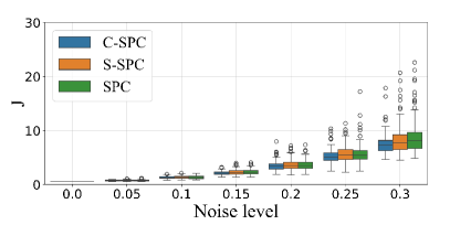
(b) $N_{d}$ = $400$

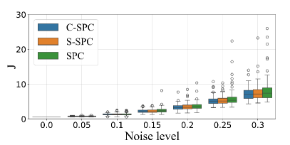
(c) $N_{d}$ = $600$

Figure 1: Control performance of C-SPC, S-SPC, and SPC of LTI system with open-loop data collection in $100$ Monte Carlo simulation.

Next, we delve into the performance of three regularized DeePC methods, i.e. RC-DeePC, RS-DeePC and R-DeePC, which are relaxations of C-SPC, S-SPC and SPC, respectively. For the clarity of comparison, we let $\lambda=\mu$ in RC-DeePC so that there is only a single parameter $\mu$ to be calibrated in three methods. By varying $\mu$ within a wide range, a continuum of control costs realized by a particular control design can be obtained. Due to the randomness of data sampling and its impact on multi-step predictor modelling, the results can be categorized into two classes with different patterns.

• Class I: A minimal control cost is achieved by using a finite $\mu$, which is lower than that without relaxation ($\mu\to\infty$), e.g. C-SPC, S-SPC and SPC.

• Class II: A minimal control cost is achieved by setting $\mu\to\infty$.

As exemplified in Fig. 2 with $N_{d}=200$ and $\sigma_{e}=0.35$, using a finite $\mu\in(10,100)$ in Class I allows the implicit predictor to differ from the one identified directly from data, thereby yielding improved control performance. A plausible explanation is that the predictor identified from data is not perfect such that even sacrificing some fitting accuracy may lead to performance improvement over non-relaxed counterparts. In the case of Class II, relaxation does not result in performance improvement. We further carry out 100 simulation runs using RC-DeePC under $N_{d}=200,400,600$ and compute the percentages of occurrence of Class I, which turn out to be $42\%$, $34\%$ and $32\%$, being decreasing with $N_{d}$. This further validates our hypothesis since with more data available, there is a higher possibility of identifying a good predictor directly from data and thus Class II appears more frequently.

The outperformance of RC-DeePC among different regularized methods with $\mu$ optimally chosen can be showcased as follows. Across 100 Monte Carlo simulations, RC-DeePC performs invariably the best under $N_{d}=200,400,600$ and $\sigma_{e}=0.35$. For a clear comparison, we normalize control costs of various methods such that the control cost of RC-DeePC is 1. The results are summarized in Table I, where the results of C-SPC, which corresponds to RC-DeePC with $\mu=\lambda=\infty$, are also reported. As $N_{d}$ increasing, the advantage of RC-DeePC over RS-DeePC and R-DeePC gradually vanishes, mainly because the lack of causality in the latter two methods can be alleviated using a larger dataset. Meanwhile, RC-DeePC outperforms C-SPC by means of regularization, and the gap becomes smaller with $N_{d}$ increasing. This showcases the usefulness of relaxation when there are no abundant data. Next, we provide a full view of performance of RC-DeePC in a single Monte Carlo run ($\sigma_{e}=0.35$, $N_{d}=200$) by varying values of $\lambda$ and $\mu$, as portrayed in Fig. 3, where the best performance can be achieved using finite $\lambda$ and $\mu$. Importantly, it suffices to set $\lambda$ and $\mu$ sufficiently large for a desirable performance, which sheds more light on better performance of RC-DeePC than that of C-SPC within Class I.

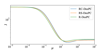
(a) Class I

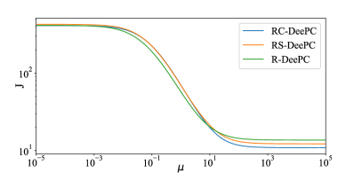
(b) Class II

Figure 2: Control performance of R-DeePC, RS-DeePC, and RC-DeePC $(\lambda=\mu)$ of LTI system with open-loop data collection ($\sigma_{e}=0.35$, $N_{d}=200$).

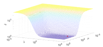
Figure 3: Control performance of RC-DeePC of LTI system with open-loop data collection ($\sigma_{e}=0.35$, $N_{d}=200$). The red star indicates that optimal performance is achieved with $\lambda=9770.1$ and $\mu=117.6812$.

TABLE I: Normalized Control Costs of Different Control Strategies of LTI System with Open-Loop Data ($\sigma_{e}=0.35$).

	$N_{d}=200$	$N_{d}=400$	$N_{d}=600$
RC-DeePC	1	1	1
RS-DeePC	1.1689	1.0970	1.0508
R-DeePC	1.3140	1.1190	1.0933
C-SPC	1.0581	1.0460	1.0214

IV-A2 Data collection under closed-loop conditions

Admittedly, the informativity of offline dataset heavily impacts the quality of multi-step predictor. In closed-loop conditions, data generated are typically prone to poor informativity, which may render the implicit predictor overfitted from data and thus poses challenges for data-driven control [38]. In this case, accounting for causality may be particularly helpful due to its effect in hedging against overfitting. To shed light onto this, we close the loop by a stabilizing controller $C(z)$, which is formulated as the following LTI system:

$$\left\{\begin{aligned} x_{c}(t+1)&=A_{c}x_{c}(t)+B_{c}[y(t)-r(t)]\\ u(t)&=C_{c}x_{c}(t)+D_{c}[y(t)-r(t)]\end{aligned}\right.$$ (34)

where $x_{c}(t)\in\mathbb{R}^{n_{c}}$ denotes internal state of the controller, and $r(t)\in\mathbb{R}^{p}$ denotes the reference signal. The system matrices of $C(z)$ are chosen as:

$$A_{c}=\begin{bmatrix}1&0\\ 0.0722&1\end{bmatrix},~{}B_{c}=\begin{bmatrix}0.2609\\ 0.164\end{bmatrix},$$

$$C_{c}=\begin{bmatrix}0.8&0.2142\end{bmatrix},~{}D_{c}=-0.07.$$

In closed-loop control, the reference $r(t)$ remains constant. We vary $\sigma_{e}$ from $0.1$ to $0.3$ in increments of $0.05$. Under each option of $\sigma_{e}$, $100$ Monte Carlo runs are carried out with $N_{d}=200$. The performance of C-SPC, S-SPC, and SPC is showcased in Fig. 4, where C-SPC outperforms the other two strategies. Notably, by further comparing Fig. 4 and Fig. 1(a) with $N_{d}=200$, the superiority of C-SPC appears to become more significant while using offline data collected in closed-loop. This bears rationality because in case of low data informativity, lacking of causality in ordinary least-squares (15) typically degrades the accuracy of multi-step predictor, which conversely highlights the necessity of causality-informed SPC.

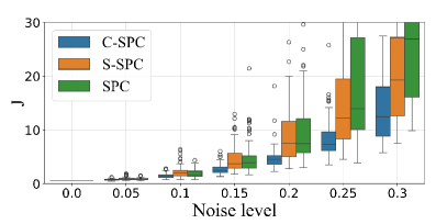
Figure 4: Control performance of C-SPC, S-SPC, and SPC of LTI system with closed-loop data collection in $100$ Monte Carlo simulation ($N_{d}=200$).

The control performance of R-DeePC, RS-DeePC, and RC-DeePC is evaluated through closed-loop data collection with $\sigma_{e}=0.35$. Using the same setup as the open-loop case, we show in Table II the normalized performance metrics of various methods with $N_{d}=200,400,600$, where RC-DeePC performs much better than the others. Meanwhile, RC-DeePC gains an upper hand over C-SPC, which showcases the benefit of using regularization for further enhancement of control performance.

TABLE II: Normalized Control Costs of Different Control Strategies of LTI System with Closed-Loop Data ($\sigma_{e}=0.35$).

	$N_{d}=200$	$N_{d}=400$	$N_{d}=600$
RC-DeePC	1	1	1
RS-DeePC	2.0411	2.6284	3.2939
R-DeePC	2.5520	2.6578	3.3114
C-SPC	1.1048	1.0843	1.0371

IV-B Data-driven control of nonlinear systems

In real-world scenarios, dynamical systems are inevitably subject to nonlinearity. Even if DeePC remains a linear predictive control scheme, its the effectiveness of DeePC in tackling nonlinear systems has been validated by a variety of empirical findings [50, 51, 16, 14], even if a wrong model class is selected. Now, we examine the efficacy of the proposed causality-informed formulation and its regularized version in nonlinear systems. We consider the following discrete-time nonlinear system:

$$\left\{\begin{aligned} x(t+1)&=Ax(t)+B\tilde{u}(t)+Ke(t)\\ y(t)&=Cx(t)+D\tilde{u}(t)+e(t)\end{aligned}\right.$$

where $\tilde{u}(t)=(1-\varepsilon)u(t)+\varepsilon[{\rm sin}(u(t))+2u^{3}(t)]$, and $\varepsilon\in[0,1]$ characterizes the degree of nonlinearity. When $\varepsilon$ is set to 0, the model dynamics is entirely linear, and the level of nonlinearity increases with $\varepsilon$. The reference to be tracked is set as a sinusoidal signal and system matrices remain the same as previous ones in LTI system.

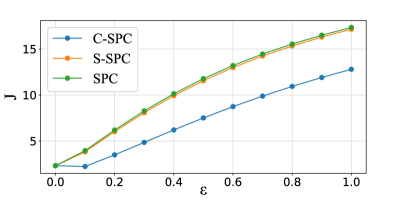
(a) $\sigma_{e}=0$

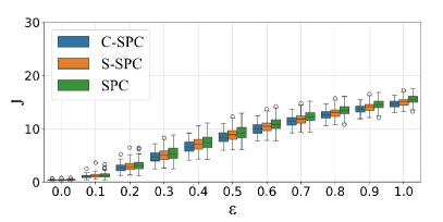
(b) $\sigma_{e}=0.05$

Figure 5: Control performance of C-SPC, S-SPC, and SPC of nonlinear system with open-loop data collection ($N_{d}=200$). Note that with $\sigma_{e}=0$, Monte Carlo simulations are no longer necessary due to the absence of uncertainty.

We collect input-output trajectories of length $N_{d}=200$ from open-loop condition to implement different data-driven control strategies. We first vary $\varepsilon$ between $0$ to $1$ in the noise-free case with $\sigma_{e}=0$, where the system becomes purely deterministic. The results of SPC, C-SPC and S-SPC are depicted in Fig. 5(a). It can be seen that the performance of all methods degrades with $\varepsilon$ increasing, while C-SPC outperforms the other methods by a large margin for $\varepsilon>0$. Very interestingly, despite the absence of uncertainty, considering causality in the implicit input-output predictor still brings obvious benefits to the realized control performance. This is indeed plausible because when a linear model class is used in SPC and S-SPC to characterize nonlinear dynamics, the implicit non-causal predictor will inevitably enclose model mismatch components in the non-causal terms, thereby leading to degraded prediction accuracy. The results in the noisy setting with $\sigma_{e}=0.05$ are further shown in Fig. 5(b), where C-SPC consistently outperforms the other two methods. This showcases that considering causality within DeePC is not only useful in reducing errors in the presence of stochastic uncertainty but also important in handling nonlinear systems. The performance of three regularized control designs that are optimally tuned along with C-SPC with $\sigma_{e}=0.3$ is also presented in Table III, where the outperformance of RC-DeePC is evident.

TABLE III: Normalized Control Costs of Different Control Strategies of Nonlinear System with Open-Loop Data ($\sigma_{e}=0.3$).

	$N_{d}=200$	$N_{d}=400$	$N_{d}=600$
RC-DeePC	1	1	1
RS-DeePC	1.2094	1.0893	1.1024
R-DeePC	1.4660	1.1674	1.1360
C-SPC	1.1113	1.0828	1.0350

V Predictive Control of A Simulated Industrial Heating Furnace

The tubular furnace is a critical equipment in petro-chemical industry, which is responsible for heating crude oil to a prescribed temperature before entering into downstream processing units [52]. As profiled in Fig. 6(a), the crude oil is heated in several spiral pipes by combustion of fuel gas. For economic and efficient combustion in the furnace, an appropriate amount of air is necessary, which is made by manipulating the inlet air flow rate, while the suitability of inlet air flow rate can be assessed by inspecting the concentration of oxygen in the stack gas. The main operational goal considered here is to make the temperature of outlet crude oil track a prescribed reference and maintain the ${\rm O}_{2}$ content of stack gas around a desired value, by manipulating flow rates of fuel gas and air.

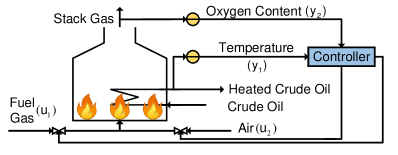
(a) Schematic diagram

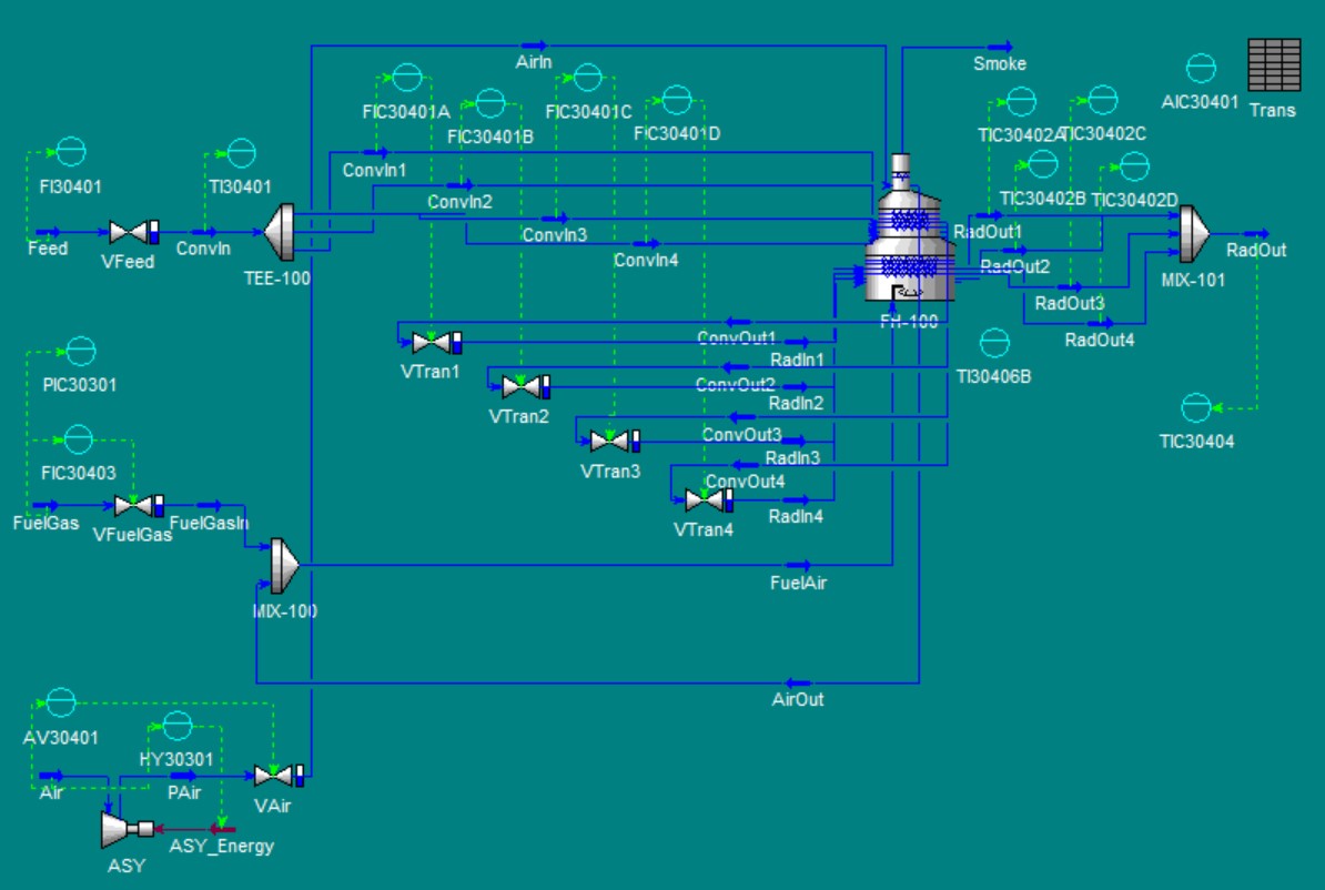
(b) Flow sheet in Honeywell UniSim Design

Figure 6: Structure of the tubular furnace.

High-fidelity simulations of the tubular furnace are enabled by using the Fired Process Heater Modeler in Honeywell UniSim Design, which is a popular process simulation software in process control, as sketched in Fig. 6(b). For control design purposes, the flow rates of fuel gas ($u_{1}$, $\text{\,}\mathrm{m}^{3}\mathrm{/}\mathrm{h}$) and air ($u_{2}$, $\text{\,}\mathrm{m}^{3}\mathrm{/}\mathrm{h}$) are chosen as the inputs, and the outlet temperature of crude oil ($y_{1}$, $\text{\,}\mathrm{\SIUnitSymbolCelsius}$) and the ${\rm O}_{2}$ content of stack gas ($y_{2}$, %) are the outputs as controlled variables. However, it is a nontrivial task to precisely describe the underlying mechanism of the tubular furnace, especially the nonlinear effect of ${\rm O}_{2}$ content together with the amount of fuel on heating efficiency. What’s more, it can be seen from Fig. 6(b) that the crude oil is split into four branches for heating, while four built-in flow controllers FIC30401A-FIC30401D are used to balance the flow in each branch and better hedge against the effect of heterogeneous combustion in the furnace. This results in a complicated external process dynamics subject to uncertainty, thereby posing a significant challenge for model-based control design. Therefore, without having to know a detailed model, it is of particular interest to implement data-driven control design of this nonlinear process.

V-A Data collection under open-loop conditions

Considering the slow dynamics of the process, data collection and control are carried out with an interval of 3 mins. To implement data-driven control strategies, an input-output trajectory $\{u_{d}(i),y_{d}(i)\}_{i=1}^{N_{d}}$ of length $N_{d}=1000$ is first collected by varying $u_{1}$ between $2740\text{\,}\mathrm{m}^{3}\mathrm{/}\mathrm{h}$ with $3160\text{\,}\mathrm{m}^{3}\mathrm{/}\mathrm{h}$ and $u_{2}$ between $30\,000\text{\,}\mathrm{m}^{3}\mathrm{/}\mathrm{h}$ with $32\,000\text{\,}\mathrm{m}^{3}\mathrm{/}\mathrm{h}$ in open-loop conditions. Data collected are then normalized to account for different scales of process variables. In online receding horizon control, the goal is to make $y_{1}$ track a varying square wave, while maintaining $y_{2}$ around $3\text{\,}\%$ for high combustion efficiency. We choose $L_{p}=50$, $L_{f}=100$, $\mathcal{Q}={\rm diag}(1_{L_{f}}\otimes[10^{-2},5\times 10^{-3}])$, and $\mathcal{R}={\rm diag}(1_{L_{f}}\otimes[10^{-4},10^{-4}])$. The constraint set $\mathbb{U}$ for inputs is designed such that $u_{1}\in[$2100\text{\,}\mathrm{m}^{3}\mathrm{/}\mathrm{h}$,$3200\text{\,}\mathrm{m}^{3}\mathrm{/}\mathrm{h}$]$ and $u_{2}\in[$24\,000\text{\,}\mathrm{m}^{3}\mathrm{/}\mathrm{h}$,$34\,000\text{\,}\mathrm{m}^{3}\mathrm{/}\mathrm{h}$]$.

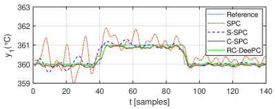
(a) Outlet temperature of crude oil

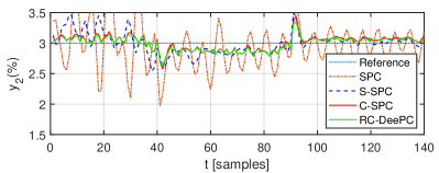
(b) ${\rm O_{2}}$ content of stack gas

Figure 7: Outputs of the tubular furnace system controlled by different controllers using open-loop data, including SPC, S-SPC, the proposed C-SPC and RC-DeePC with $\lambda=5\times 10^{-3}$ and $\mu=0.1$.

TABLE IV: Control Performance Metrics of Different Control Strategies with Open-Loop Data.

	$\mathbb{E}\{\|y_{1}(t)-r_{1}(t)\|_{2}^{2}\}$	$\mathbb{E}\{\|y_{2}(t)-r_{2}(t)\|_{2}^{2}\}$	$\mathbb{E}\{\|u_{1}(t)\|_{2}^{2}\}$	$\mathbb{E}\{\|u_{2}(t)\|_{2}^{2}\}$
SPC	0.2076	0.6081	11.685	4.031
S-SPC	0.0318	0.1271	12.163	4.193
C-SPC	0.0199	0.0611	12.615	4.449
RC-DeePC	0.0148	0.0517	12.293	4.329

The process outputs under different data-driven control strategies, including SPC, S-SPC, C-SPC and RC-DeePC, are shown in Fig. 7, and empirical performance metrics such as average tracking errors and control costs are detailed in Table IV. It can be observed that SPC yields oscillatory tracking behavior that is much less desirable than S-SPC and C-SPC, indicating that considering causality can indeed improve the control performance. Meanwhile, the tracking performance of C-SPC is superior to that of S-SPC due to a strictly causal predictor identified from data. Besides, RC-DeePC performs better than the C-SPC, which showcases the benefit of using finite regularization parameters $\lambda$ and $\mu$ in improving the control performance of this nonlinear process. The results in Table IV further indicates that C-SPC and RC-DeePC yield a desirable tracking performance by accounting for causality.

V-B Data collection under closed-loop conditions

In industrial practice, one may not be allowed to operate the process in open-loop. A practically relevant scenario is that for safety or efficiency concerns, the process has to be operated in closed-loop conditions, but practitioners may be interested in designing a data-driven predictive controller to pursue better control performance.

To ensure process safety, we assume that the loop is closed by a coarsely tuned stabilizing PI controller $C(z)$ in form of (34), whose parameters are given by:

$$A_{c}=\begin{bmatrix}1&0\\ 1&0\end{bmatrix},~{}B_{c}=\begin{bmatrix}0.0802&0\\ 0.2990&0\end{bmatrix},$$

$$C_{c}=\begin{bmatrix}1&0\\ 1&0\end{bmatrix},~{}D_{c}=\begin{bmatrix}0.3260&0\\ 0.6250&0\end{bmatrix}.$$

Under closed-loop feedback control, an input-output trajectory of length $N_{d}=2000$ is generated by varying the setpoint of $y_{1}$ between $360\text{\,}\mathrm{\SIUnitSymbolCelsius}$ and $366\text{\,}\mathrm{\SIUnitSymbolCelsius}$ and that of $y_{2}$ between $1.5\text{\,}\%$ and $2.5\text{\,}\%$. In online predictive control, the reference of $y_{1}$ is a square wave varying between $363\text{\,}\mathrm{\SIUnitSymbolCelsius}$ and $364\text{\,}\mathrm{\SIUnitSymbolCelsius}$, while a constant reference is set for $y_{2}$. For data-driven predictive controller design, we set $\mathcal{Q}={\rm diag}(1_{L_{f}}\otimes[10^{-3},5\times 10^{-3}])$ and $\mathcal{R}={\rm diag}(1_{L_{f}}\otimes[10^{-4},10^{-4}])$, while the other parameters are the same as those in the previous open-loop case.

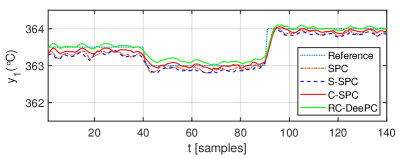
(a) Outlet temperature of crude oil

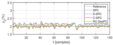
(b) ${\rm O_{2}}$ content of stack gas

Figure 8: Outputs of the tubular furnace system controlled by different controllers using closed-loop data, including SPC, S-SPC, the proposed C-SPC and RC-DeePC.

TABLE V: Control Performance Metrics of Different Control Strategies with Closed-Loop Data.

	$\mathbb{E}\{\|y_{1}(t)-r_{1}(t)\|_{2}^{2}\}$	$\mathbb{E}\{\|y_{2}(t)-r_{2}(t)\|_{2}^{2}\}$	$\mathbb{E}\{\|u_{1}(t)\|_{2}^{2}\}$	$\mathbb{E}\{\|u_{2}(t)\|_{2}^{2}\}$
SPC	0.0235	0.0527	1.6463	1.4371
S-SPC	0.0325	0.0819	1.6930	1.3320
C-SPC	0.0123	0.0183	1.5110	1.7562
RC-DeePC	0.0123	0.0148	1.3039	1.3625

We implement four data-driven control schemes, including SPC, S-SPC, C-SPC, and RC-DeePC, to investigate their realized performance of the simulated tubular furnace. In RC-DeePC, the regularization parameters are chosen as $\lambda=5\times 10^{-3}$ and $\mu=0.1$. The controlled outputs are depicted in Fig. 8. Empirical performance metrics, such as average tracking errors and control costs, can be found in Table V. It can be seen that S-SPC exhibits an even less favorable tracking than SPC, whereas C-SPC exhibits better performance than SPC due to the enforced causality. In addition, the regularized formulation RC-DeePC, as a relaxation of C-SPC, gains the upper hand over C-SPC, in terms of less tracking errors and remarkably reduced control costs. This showcases the usefulness of enforcing a causal predictive relation in data-driven control, based on which regularizaion may bring further benefit.

VI Conclusion

In this paper, a novel causality-informed formulation of DeePC was derived by means of LQ factorization, which can lead to remarkably improved performance over the existing DeePC methodology that falls short of considering causality. To achieve this goal, we first revisited the two-stage formulation of DeePC using LQ factorization [33], and established the equivalence between its regularized version and R-DeePC in [27]. This yields a unified framework for data-driven control with clear interpretability and compatibility with regularization. On this basis, a simple two-stage formulation of causality-informed DeePC is developed, which only requires block-triangularization of a submatrix in the LQ factorization as compared to the generic two-stage formulation in [33]. Thus, the proposed new causality-informed formulation is as easy to solve as the two-stage formulation. Furthermore, a regularized reformulation was derived that balances between control cost minimization and implicit identification of multi-step predictors, which can bring further performance improvement. Numerical examples and applications to a simulated industrial furnace system were presented to demonstrate the significantly improved performance of the causality-informed data-driven control formulation, in the presence of not only stochastic noise but also insufficient data informativity and process nonlinearity.

Appendix: Proof of Theorem 3

We first assume that $\begin{bmatrix}\gamma^{\top}_{1}&\gamma^{\top}_{2}&\gamma^{\top}_{3}\end{bmatrix}^{\top}$ along with $u_{f}$ and $\hat{y}_{f}$ yields a feasible solution to (12), and then construct a candidate solution $g=\sum^{3}_{i=1}Q^{\top}_{i}\gamma_{i}$ to (13). According to the relation in (10), one obtains:

$$\begin{split}\begin{bmatrix}z_{p}\\ u_{f}\\ \hat{y}_{f}\end{bmatrix}=&\begin{bmatrix}L_{11}&0&0\\ L_{21}&L_{22}&0\\ L_{31}&L_{32}&L_{33}\end{bmatrix}\begin{bmatrix}\gamma_{1}\\ \gamma_{2}\\ \gamma_{3}\\ \end{bmatrix}\\ =&\begin{bmatrix}L_{11}&0&0\\ L_{21}&L_{22}&0\\ L_{31}&L_{32}&L_{33}\end{bmatrix}\begin{bmatrix}Q_{1}\\ Q_{2}\\ Q_{3}\\ \end{bmatrix}g\\ =&\begin{bmatrix}Z_{p}\\ U_{f}\\ {Y}_{f}\end{bmatrix}g,\end{split}$$

which indicates that $\{g,u_{f},\hat{y}_{f}\}$ satisfies (13b) and (13c). Next, we further show that the feasible solution $\begin{bmatrix}\gamma^{\top}_{1}&\gamma^{\top}_{2}&\gamma^{\top}_{3}\end{bmatrix}^{\top}$ to (12) and $g$ to (13) have same objective values. It can be easily proven by LQ factorization (9) that the psuedo inverse is given by:

$$\begin{bmatrix}Z_{p}\\ U_{f}\end{bmatrix}^{\dagger}=\begin{bmatrix}Q_{1}\\ Q_{2}\end{bmatrix}^{\top}\begin{bmatrix}L_{11}&0\\ L_{21}&L_{22}\end{bmatrix}^{-1}.$$ (35)

Using (35) and orthonormal properties of $\{Q_{i}\}_{i=1}^{3}$, we obtain:

$$\Pi g= \begin{bmatrix}Q_{1}\\ Q_{2}\end{bmatrix}^{\top}\begin{bmatrix}\gamma_{1}\\ \gamma_{2}\end{bmatrix}.$$

It then follows that

$$(I-\Pi)g =g-\Pi g$$

$$=\begin{bmatrix}Q_{1}\\ Q_{2}\end{bmatrix}^{\top}\begin{bmatrix}\gamma_{1}\\ \gamma_{2}\end{bmatrix}+Q_{3}^{\top}\gamma_{3}-\begin{bmatrix}Q_{1}\\ Q_{2}\end{bmatrix}^{\top}\begin{bmatrix}\gamma_{1}\\ \gamma_{2}\end{bmatrix}$$

$$=Q^{\top}_{3}\gamma_{3},$$

which indicates that $\|(I-\Pi)g\|^{2}=\|Q^{\top}_{3}\gamma_{3}\|^{2}=\|\gamma_{3}\|^{2}$ due to $Q_{3}Q^{\top}_{3}=I$. In summary, given any feasible solution $\begin{bmatrix}\gamma^{\top}_{1}&\gamma^{\top}_{2}&\gamma^{\top}_{3}\end{bmatrix}^{\top}$ to (12), there always exists a feasible solution $g$ to (13) such that they have same objective values.

Then we assume that $\{g,u_{f},\hat{y}_{f}\}$ is a feasible solution to (13). Let $Q=[Q_{1}^{\top}~{}Q_{2}^{\top}~{}Q_{3}^{\top}~{}Q_{4}^{\top}]$ be an orthogonal matrix satisfying $QQ^{\top}=I$, such that its row space forms a set of complete bases and $g$ can be expressed uniquely as $g=Q^{\top}_{1}\pi_{1}+Q^{\top}_{2}\pi_{2}+Q^{\top}_{3}\pi_{3}+Q^{\top}_{4}\pi_{4}$. To construct a feasible solution to (12) conversely, we first construct an alternative feasible solution $\{g^{\prime},u_{f},\hat{y}_{f}\}$ to (13), where $g^{\prime}=Q^{\top}_{1}\pi_{1}+Q^{\top}_{2}\pi_{2}+Q^{\top}_{3}\pi_{3}$ provably satisfies (13b) in virtue of the LQ factorization. Meanwhile, both $\{g^{\prime},u_{f},\hat{y}_{f}\}$ and $\{g,u_{f},\hat{y}_{f}\}$ have the same control cost $\mathcal{J}(u_{f},\hat{y}_{f})$, while $\|(I-\Pi)g^{\prime}\|^{2}<\|(I-\Pi)g\|^{2}$ holds for $\pi_{4}\neq 0$. Letting $\gamma_{i}=\pi_{i},~{}i=1,2,3$, we then show that $\{\gamma,u_{f},\hat{y}_{f}\}$ is feasible to (12) and has the same objective value as $\{g^{\prime},u_{f},\hat{y}_{f}\}$. Note that

$$\begin{split}\begin{bmatrix}z_{p}\\ u_{f}\\ \hat{y}_{f}\\ \end{bmatrix}=\begin{bmatrix}Z_{p}\\ U_{f}\\ {Y}_{f}\end{bmatrix}g^{\prime}=\begin{bmatrix}L_{11}&0&0\\ L_{21}&L_{22}&0\\ L_{31}&L_{32}&L_{33}\\ \end{bmatrix}\begin{bmatrix}\pi_{1}\\ \pi_{2}\\ \pi_{3}\end{bmatrix},\end{split}$$

which indicates $\{\gamma,u_{f},\hat{y}_{f}\}$ fulfills (12b). Using a similar argument as above, one can readily show that $\{\gamma,u_{f},\hat{y}_{f}\}$ and $\{g^{\prime},u_{f},\hat{y}_{f}\}$ lead to the same control cost as well as the penalty value. Thus, given any feasible solution $\{g,u_{f},\hat{y}_{f}\}$, there always exists $\{g^{\prime},u_{f},\hat{y}_{f}\}$ that is no worse than $\{g,u_{f},\hat{y}_{f}\}$ and exactly corresponds to a feasible solution $\{\gamma,u_{f},\hat{y}_{f}\}$ to (12). Combining the above arguments finishes the proof of Theorem 3.

References

- [1] S. J. Qin and T. A. Badgwell, “An overview of industrial model predictive control technology,” in AIche symposium series, vol. 93, no. 316. New York, NY: American Institute of Chemical Engineers, 1971-c2002., 1997, pp. 232–256.
- [2] M. Morari and J. H. Lee, “Model predictive control: past, present and future,” Computers & chemical engineering, vol. 23, no. 4-5, pp. 667–682, 1999.
- [3] S. J. Qin and T. A. Badgwell, “A survey of industrial model predictive control technology,” Control Engineering Practice, vol. 11, no. 7, pp. 733–764, 2003.
- [4] J. B. Rawlings, D. Q. Mayne, and M. Diehl, Model predictive control: theory, computation, and design. Nob Hill Publishing Madison, WI, 2017, vol. 2.
- [5] M. Gevers, “Identification for control: From the early achievements to the revival of experiment design,” European Journal of Control, vol. 11, no. 4-5, pp. 335–352, 2005.
- [6] I. Markovsky, “A software package for system identification in the behavioral setting,” Control Engineering Practice, vol. 21, no. 10, pp. 1422–1436, 2013.
- [7] H. Hjalmarsson, M. Gevers, and F. De Bruyne, “For model-based control design, closed-loop identification gives better performance,” Automatica, vol. 32, no. 12, pp. 1659–1673, 1996.
- [8] C. Shang, W.-H. Chen, A. D. Stroock, and F. You, “Robust model predictive control of irrigation systems with active uncertainty learning and data analytics,” IEEE Transactions on Control Systems Technology, vol. 28, no. 4, pp. 1493–1504, 2020.
- [9] J. Coulson, J. Lygeros, and F. Dörfler, “Data-enabled predictive control: In the shallows of the DeePC,” in 2019 18th European Control Conference (ECC). IEEE, 2019, pp. 307–312.
- [10] M. Yin, A. Iannelli, and R. S. Smith, “Maximum likelihood estimation in data-driven modeling and control,” IEEE Transactions on Automatic Control, vol. 68, no. 1, pp. 317–328, 2023.
- [11] W. Favoreel, B. De Moor, and M. Gevers, “SPC: Subspace predictive control,” IFAC Proceedings Volumes, vol. 32, no. 2, pp. 4004–4009, 1999.
- [12] L. Huang, J. Coulson, J. Lygeros, and F. Dörfler, “Decentralized data-enabled predictive control for power system oscillation damping,” IEEE Transactions on Control Systems Technology, vol. 30, no. 3, pp. 1065–1077, 2021.
- [13] D. Bilgic, A. Koch, G. Pan, and T. Faulwasser, “Toward data-driven predictive control of multi-energy distribution systems,” Electric Power Systems Research, vol. 212, p. 108311, 2022.
- [14] E. Elokda, J. Coulson, P. N. Beuchat, J. Lygeros, and F. Dörfler, “Data-enabled predictive control for quadcopters,” International Journal of Robust and Nonlinear Control, vol. 31, no. 18, pp. 8916–8936, 2021.
- [15] R. T. Fawcett, K. Afsari, A. D. Ames, and K. A. Hamed, “Toward a data-driven template model for quadrupedal locomotion,” IEEE Robotics and Automation Letters, vol. 7, no. 3, pp. 7636–7643, 2022.
- [16] P. G. Carlet, A. Favato, S. Bolognani, and F. Dörfler, “Data-driven predictive current control for synchronous motor drives,” in 2020 IEEE Energy Conversion Congress and Exposition. IEEE, 2020, pp. 5148–5154.
- [17] V. Chinde, Y. Lin, and M. J. Ellis, “Data-enabled predictive control for building HVAC systems,” Journal of Dynamic Systems, Measurement, and Control, vol. 144, no. 8, p. 081001, 2022.
- [18] Y. Lian, J. Shi, M. Koch, and C. N. Jones, “Adaptive robust data-driven building control via bilevel reformulation: An experimental result,” IEEE Transactions on Control Systems Technology, vol. 31, no. 6, pp. 2420–2436, 2023.
- [19] L. Schmitt, J. Beerwerth, M. Bahr, and D. Abel, “Data-driven predictive control with online adaption: Application to a fuel cell system,” IEEE Transactions on Control Systems Technology, DOI:10.1109/TCST.2023.3293790, 2023.
- [20] I. Markovsky and F. Dörfler, “Behavioral systems theory in data-driven analysis, signal processing, and control,” Annual Reviews in Control, vol. 52, pp. 42–64, 2021.
- [21] J. C. Willems, “Paradigms and puzzles in the theory of dynamical systems,” IEEE Transactions on Automatic Control, vol. 36, no. 3, pp. 259–294, 1991.
- [22] ——, “The behavioral approach to open and interconnected systems,” IEEE control systems magazine, vol. 27, no. 6, pp. 46–99, 2007.
- [23] J. C. Willems and J. W. Polderman, Introduction to Mathematical Systems Theory: A Behavioral Approach. Springer Science & Business Media, 1997, vol. 26.
- [24] T. Martin, T. B. Schön, and F. Allgöwer, “Guarantees for data-driven control of nonlinear systems using semidefinite programming: A survey,” Annual Reviews in Control, p. 100911, 2023.
- [25] V. Krishnan and F. Pasqualetti, “On direct vs indirect data-driven predictive control,” in 2021 60th IEEE Conference on Decision and Control. IEEE, 2021, pp. 736–741.
- [26] F. Fiedler and S. Lucia, “On the relationship between data-enabled predictive control and subspace predictive control,” in 2021 European Control Conference (ECC). IEEE, 2021, pp. 222–229.
- [27] F. Dörfler, J. Coulson, and I. Markovsky, “Bridging direct & indirect data-driven control formulations via regularizations and relaxations,” IEEE Transactions on Automatic Control, vol. 68, no. 2, pp. 883–897, 2023.
- [28] J. Berberich, C. W. Scherer, and F. Allgöwer, “Combining prior knowledge and data for robust controller design,” IEEE Transactions on Automatic Control, vol. 68, no. 8, pp. 4618–4633, 2023.
- [29] S. J. Qin and L. Ljung, “Closed-loop subspace identification with innovation estimation,” IFAC Proceedings Volumes, vol. 36, no. 16, pp. 861–866, 2003.
- [30] S. J. Qin, W. Lin, and L. Ljung, “A novel subspace identification approach with enforced causal models,” Automatica, vol. 41, no. 12, pp. 2043–2053, 2005.
- [31] B. Huang and R. Kadali, “Dynamic modeling, predictive control and performance monitoring: A data-driven subspace approach,” Springer, 2008.
- [32] E. O’Dwyer, E. C. Kerrigan, P. Falugi, M. Zagorowska, and N. Shah, “Data-driven predictive control with improved performance using segmented trajectories,” IEEE Transactions on Control Systems Technology, vol. 31, no. 3, pp. 1355–1365, 2023.
- [33] V. Breschi, A. Chiuso, and S. Formentin, “Data-driven predictive control in a stochastic setting: A unified framework,” Automatica, vol. 152, p. 110961, 2023.
- [34] J. C. Willems, P. Rapisarda, I. Markovsky, and B. L. De Moor, “A note on persistency of excitation,” Systems & Control Letters, vol. 54, no. 4, pp. 325–329, 2005.
- [35] S. Sedghizadeh and S. Beheshti, “Data-driven subspace predictive control: Stability and horizon tuning,” Journal of the Franklin Institute, vol. 355, no. 15, pp. 7509–7547, 2018.
- [36] E. T. Hale and S. J. Qin, “Subspace model predictive control and a case study,” in Proceedings of the 2002 American Control Conference, vol. 6. IEEE, 2002, pp. 4758–4763.
- [37] V. Vajpayee, S. Mukhopadhyay, and A. P. Tiwari, “Data-driven subspace predictive control of a nuclear reactor,” IEEE Transactions on Nuclear Science, vol. 65, no. 2, pp. 666–679, 2017.
- [38] J. Dong, M. Verhaegen, and E. Holweg, “Closed-loop subspace predictive control for fault tolerant MPC design,” IFAC Proceedings Volumes, vol. 41, no. 2, pp. 3216–3221, 2008.
- [39] J. Cigler and S. Prívara, “Subspace identification and model predictive control for buildings,” in 2010 11th International Conference on Control Automation Robotics & Vision. IEEE, 2010, pp. 750–755.
- [40] V. Breschi, M. Fabris, S. Formentin, and A. Chiuso, “Uncertainty-aware data-driven predictive control in a stochastic setting,” arXiv preprint arXiv:2211.10321, 2022.
- [41] V. Breschi, A. Chiuso, M. Fabris, and S. Formentin, “On the impact of regularization in data-driven predictive control,” arXiv preprint arXiv:2304.00263, 2023.
- [42] M. Lazar and P. Verheijen, “Generalized data–driven predictive control: Merging subspace and Hankel predictors,” Mathematics, vol. 11, no. 9, p. 2216, 2023.
- [43] J. Berberich, J. Köhler, M. A. Müller, and F. Allgöwer, “Data-driven model predictive control with stability and robustness guarantees,” IEEE Transactions on Automatic Control, vol. 66, no. 4, pp. 1702–1717, 2021.
- [44] S. Formentin and A. Chiuso, “Core: Control-oriented regularization for system identification,” in 2018 IEEE Conference on Decision and Control (CDC). IEEE, 2018, pp. 2253–2258.
- [45] R. Shi and J. F. MacGregor, “A framework for subspace identification methods,” in Proceedings of the 2001 American Control Conference, vol. 5. IEEE, 2001, pp. 3678–3683.
- [46] G. Van der Veen, J.-W. van Wingerden, M. Bergamasco, M. Lovera, and M. Verhaegen, “Closed-loop subspace identification methods: An overview,” IET Control Theory & Applications, vol. 7, no. 10, pp. 1339–1358, 2013.
- [47] A. Bemporad, M. Morari, V. Dua, and E. N. Pistikopoulos, “The explicit linear quadratic regulator for constrained systems,” Automatica, vol. 38, no. 1, pp. 3–20, 2002.
- [48] Gurobi Optimization, LLC, “Gurobi optimizer reference manual,” 2023. [Online]. Available: https://www.gurobi.com
- [49] J. Löfberg, “YALMIP: A toolbox for modeling and optimization in MATLAB,” in 2004 IEEE International Conference on Robotics and Automation, 2004, pp. 284–289.
- [50] L. Huang, J. Zhen, J. Lygeros, and F. Dörfler, “Quadratic regularization of data-enabled predictive control: Theory and application to power converter experiments,” IFAC-PapersOnLine, vol. 54, no. 7, pp. 192–197, 2021.
- [51] ——, “Robust data-enabled predictive control: Tractable formulations and performance guarantees,” IEEE Transactions on Automatic Control, vol. 68, no. 5, pp. 3163–3170, 2023.
- [52] Z. Zeybek, “Role of adaptive heuristic criticism in cascade temperature control of an industrial tubular furnace,” Applied Thermal Engineering, vol. 26, no. 2-3, pp. 152–160, 2006.