Entanglement constraint on wave-particle duality for tripartite systems

Abstract

A global multi-partite entanglement may place a constraint on the wave-particle duality. We investigate this constraint relation of the global entanglement and the quantitative wave-particle duality in tripartite systems. We perform quantum state tomography to reconstruct the reduced density matrix by using the OriginQ quantum computing cloud platform. As a result, we show that, theoretically and experimentally, the quantitative wave-particle duality is indeed constrained by the global tripartite entanglement.

1 Introduction

The principle of wave-particle duality plays an important role in quantum physics. In 1924, De Broglie Ph.D.thesis(1925) first proposed the hypothesis of matter wave, which is intrinsically related to the Bohr complementarity principle Nature.121.580(1928) and the Heisenberg uncertainty relation Z.Phys.33.879(1925) . In recent years, with the development of quantum physics, especially quantum information theory, how to quantify the wave-particle duality has received the most attention.

In 1979, Wootters and Zurek PhysRevD.19.473(1979) first investigated the problem of quantifying wave-particle duality. Soon afterward Greenberger and Yasin Phys.Lett.A.128.391(1988) proposed a duality relation $P^{2}+V^{2}=1$ for the pure state of a single particle, where $P$ is path predictability characterizing particleness, and $V$ is the amount of interference describing waviness. Also, Englert Phys.Rev.Lett.77.2154(1996) derived $D^{2}+V^{2}\leq 1$, where $D$ denotes path distinguishability to quantify the particleness and $V$ is fringe visibility to quantify the waviness. Since then, other interesting aspects of quantifying wave-particle duality have been investigated, such as asymmetric beams Proc.R.Soc.A.468.1065(2012) ; Phys.Rev.A.98.022130(2018) , multi-slit interference Phys.Rev.A.64.042113(2001) ; Int.J.Quant.Inf.6.129(2008) ; Phys.Rev.A.92.012118(2015) ; Phys.Rev.A.93.062111(2016) , etc. These studies mainly focus on the case of the single particle.

For bipartite systems, it is found that one should consider three quantities $P$, $V$ and the entanglement measure between two particles Phys.Rev.A.48.1023(1993) ; Phys.Rev.A.51.54(1995) . Typically, Jakob and Bergou Opt.Commun.283.827(2010) have reported a triality relation for the bipartite system as $P^{2}+V^{2}+C^{2}=1$, where $C$ is the well-known bipartite entanglement measure, concurrence. So far, the research on the triality relation for bipartite systems has achieved fruitful results Phys.Rev.A.76.052107(2007) ; Phys.Rev.A.103.022409(2021) ; Opt.Lett.46.492(2021) . For multi-partite systems, more recently, Marrou josaa.40.4.c22(2023) et al. designed the experimental tests to show the triality relations using coupled photons involving the polarization and the spatial degrees of freedom. However, such relations were constrained only by the concurrence rather than the global tripartite entanglement.

In this paper, we focus on quantifying wave-particle duality constrained by the global tripartite entanglement. Based on quantum state tomography, we design quantum circuit to test the constraint relation by using the OriginQ quantum computing cloud platform.

2 Quantitative wave-particle duality

For a single qubit system, the quantum state can be represented by the density matrix

$$\rho=\left(\begin{array}[]{cc}\rho_{11}&~{}\rho_{12}\\ \rho_{21}&~{}\rho_{22}\\ \end{array}\right).$$ (3)

Density matrix $\rho$ can be used to characterize waviness and particleness Phys.Rev.A.64.042113(2001) , namely, visibility and predictability.

The visibility is usually defined by

$$V=2|\rho_{12}|.$$ (4)

It is related to non-diagonal elements of the density matrix under two orthogonal bases $|0\rangle$ and $|1\rangle$, and it measures the waviness for the single qubit systems. While for the particleness, it can always be measured by the diagonal elements of the density matrix, that is, the predictability

$$P=|\rho_{22}-\rho_{11}|$$ (5)

introduced in the two-beam interferometers Phys.Lett.A.128.391(1988) ; Phys.Rev.Lett.77.2154(1996) .

More generally, for multipartite systems, the waviness and particleness of the $k$-th subsystem obey the same rules as single-qubit Opt.Commun.283.827(2010) ; Phys.Rev.A.103.022409(2021) . One can express them as

$$V_{k}=2|\rho_{k_{12}}|$$ (6)

and

$$P_{k}=|\rho_{k_{22}}-\rho_{k_{11}}|,$$ (7)

where $\rho_{k}$ is the reduced density matrix of the $k$-th subsystem.

3 Tripartite entanglement constraint on wave-particle duality

Consider the tripartite systems consisting of three qubits, i.e., $A$, $B$ and $C$, and an arbitrary pure state of such systems can be expressed as

$$\begin{split}|\psi_{ABC}\rangle=&a|000\rangle+b|001\rangle+c|010\rangle+d|100\rangle+e|110\rangle+f|101\rangle\ \\ &+g|011\rangle+h|111\rangle,\end{split}$$ (8)

where $a,b,c,d,e,f,g,h$ are complex numbers satisfying $|a|^{2}+|b|^{2}+|c|^{2}+|d|^{2}+|e|^{2}+|f|^{2}+|g|^{2}+|h|^{2}=1$. The density matrix of the state $|\psi_{ABC}\rangle$ is

$$\rho_{ABC} =|\psi_{ABC}\rangle\langle\psi_{ABC}|$$ (9)

and the reduced density matrices of the subsystems $A$, $B$ and $C$ are respectively

$$\begin{split}\rho_{A}&=\textrm{Tr}_{BC}(\rho_{ABC})\ \\ &=\left(\begin{array}[]{cc}aa^{*}+bb^{*}+cc^{*}+gg^{*}&~{}ad^{*}+bf^{*}+ce^{*}+gh^{*}\\ a^{*}d+b^{*}f+c^{*}e+g^{*}h&~{}dd^{*}+ee^{*}+ff^{*}+hh^{*}\\ \end{array}\right),\end{split}$$ (10)

$$\begin{split}\rho_{B}&=\textrm{Tr}_{AC}(\rho_{ABC})\ \\ &=\left(\begin{array}[]{cc}aa^{*}+bb^{*}+dd^{*}+ff^{*}&~{}ac^{*}+bg^{*}+de^{*}+fh^{*}\\ a^{*}c+b^{*}g+d^{*}e+f^{*}h&~{}cc^{*}+ee^{*}+gg^{*}+hh^{*}\\ \end{array}\right)\end{split}$$ (11)

and

$$\begin{split}\rho_{C}&=\textrm{Tr}_{AB}(\rho_{ABC})\ \\ &=\left(\begin{array}[]{cc}aa^{*}+cc^{*}+dd^{*}+ee^{*}&~{}ab^{*}+cg^{*}+df^{*}+eh^{*}\\ a^{*}b+c^{*}g+d^{*}f+e^{*}h&~{}bb^{*}+ff^{*}+gg^{*}+hh^{*}\\ \end{array}\right).\end{split}$$ (12)

We calculate $V_{k}$ and $P_{k}$, respectively, and we have

$$V_{A} =2|ad^{*}+bf^{*}+ce^{*}+gh^{*}|,$$ (13)

$$V_{B} =2|ac^{*}+bg^{*}+de^{*}+fh^{*}|,$$ (14)

$$V_{C} =2|ab^{*}+cg^{*}+df^{*}+eh^{*}|,$$ (15)

$$P_{A}=||d|^{2}+|e|^{2}+|f|^{2}+|h|^{2}-|a|^{2}-|b|^{2}-|c|^{2}-|g|^{2}|,$$ (16)

$$P_{B}=||c|^{2}+|e|^{2}+|g|^{2}+|h|^{2}-|a|^{2}-|b|^{2}-|d|^{2}-|f|^{2}|$$ (17)

and

$$P_{C}=||b|^{2}+|f|^{2}+|g|^{2}+|h|^{2}-|a|^{2}-|c|^{2}-|d|^{2}-|e|^{2}|.$$ (18)

Then it is not difficult to check that

$$\sum_{k=A,B,C}(V_{k}^{2}+P_{k}^{2})\leq 3.$$ (19)

This means that these quantities, like $V_{k}$ and $P_{k}$, that are associated with the waviness and particleness of the subsystems can be constrained by such an inequality. In order to build up a complete description of wave-particle duality for tripartite systems with equality rather than inequality, just as for bipartite systems Opt.Commun.283.827(2010) , it is natural to think of the tripartite entanglement.

Here we consider the multi-partite entanglement measure J.Math.Phys.43.4273(2002) ; 0305094 $Q=2[1-\frac{1}{n}\sum_{k=0}^{n-1}\textrm{Tr}(\rho_{k}^{2})]$, where $\rho_{k}$ is the reduced density matrix of the $k$-th subsystem of the combined system $\rho$. Let $n=3$, then for the state $|\psi_{ABC}\rangle$ we have

$$Q=\frac{2}{3}[3-\textrm{Tr}(\rho_{A}^{2})-\textrm{Tr}(\rho_{B}^{2})-\textrm{Tr}(\rho_{C}^{2})].$$ (20)

A straightforward calculation using Eqs.(13)-(18) shows that

$$Q+\frac{1}{3}\sum_{k=A,B,C}V_{k}^{2}+\frac{1}{3}\sum_{k=A,B,C}P_{k}^{2}=1.$$ (21)

This leads to the conclusion that there exists a constraint relation of the global tripartite entanglement, quantitative waviness and particleness for the tripartite systems. Thus, one can argue that indeed the quantities associated with the waviness and particleness of the subsystems are constrained by the “global entanglement”.

4 Experimental test of the triality relation

We next verify the present constraint relation for tripartite systems by means of quantum state tomography.

4.1 Quantum state tomography

Quantum state tomography Phys.RevA.64.052312.(2001) is an effective method for determining the state of a quantum system. It uses projective measurements on a collection of identically prepared systems and then it is capable of reconstructing the density matrix of the unknown quantum system.

For a single qubit, select a set of measurement operators $\mu_{0}=|0\rangle\langle 0|+|1\rangle\langle 1|$, $\mu_{1}=|0\rangle\langle 0|$, $\mu_{2}=|-\rangle\langle-|$ and $\mu_{3}=|R\rangle\langle R|$, where $|-\rangle=(|0\rangle-|1\rangle)/\sqrt{2}$ and $|R\rangle=(|0\rangle-\textrm{i}|1\rangle)/\sqrt{2}$. These four measurements are respectively related by the counts $n_{0}=N/2(\langle 0|\rho|0\rangle+\langle 1|\rho|1\rangle)$, $n_{1}=N\langle 0|\rho|0\rangle$, $n_{2}=N\langle-|\rho|-\rangle$ and $n_{3}=N\langle R|\rho|R\rangle$, where $N$ is a constant on the experimental configuration. By this, it will suffice to reconstruct single qubit state as

$$\rho =\frac{1}{2}\sum^{3}_{i=0}\frac{S_{i}}{S_{0}}\sigma_{i},$$ (22)

where $S_{0}=2n_{0}$, $S_{1}=2(n_{1}-n_{0})$, $S_{2}=2(n_{2}-n_{0})$ and $S_{3}=2(n_{3}-n_{0})$ are the Stokes parameters, and $\sigma_{0}=|R\rangle\langle R|+|L\rangle\langle L|$, $\sigma_{1}=|R\rangle\langle L|+|L\rangle\langle R|$, $\sigma_{2}=\textrm{i}(|L\rangle\langle R|-|R\rangle\langle L|)$ and $\sigma_{3}=|R\rangle\langle R|-|L\rangle\langle L|$ are the Pauli matrices. Here $|L\rangle=(|0\rangle+\textrm{i}|1\rangle)/\sqrt{2}$.

4.2 Experimental test using OriginQ quantum computer

OriginQ offers a cloud platform to carry out quantum calculation with superconducting quantum computers OriginQ . We now turn to the experimental test of the constraint relation on the quantum cloud platform.

First, consider the states of tripartite systems

$$|\psi\rangle_{ABC}= \cos\frac{\theta_{1}}{2}\cos\frac{\theta_{2}}{2}\cos\frac{\theta_{3}}{2}|000\rangle+\cos\frac{\theta_{1}}{2}\cos\frac{\theta_{2}}{2}\sin\frac{\theta_{3}}{2}|001\rangle$$ (23)

$$+\cos\frac{\theta_{1}}{2}\sin\frac{\theta_{2}}{2}\cos\frac{\theta_{3}}{2}|010\rangle+\sin\frac{\theta_{1}}{2}\sin\frac{\theta_{2}}{2}\sin\frac{\theta_{3}}{2}|100\rangle$$

$$+\cos\frac{\theta_{1}}{2}\sin\frac{\theta_{2}}{2}\sin\frac{\theta_{3}}{2}|011\rangle+\sin\frac{\theta_{1}}{2}\cos\frac{\theta_{2}}{2}\sin\frac{\theta_{3}}{2}|110\rangle$$

$$+\sin\frac{\theta_{1}}{2}\sin\frac{\theta_{2}}{2}\cos\frac{\theta_{3}}{2}|101\rangle+\sin\frac{\theta_{1}}{2}\cos\frac{\theta_{2}}{2}\cos\frac{\theta_{3}}{2}|111\rangle,$$

which can be prepared by using the rotation operators $R_{y}(\theta_{i})=\left(\begin{array}[]{cc}\cos{\theta_{i}}/{2}&-\sin{\theta_{i}}/{2}\\ \sin{\theta_{i}}/{2}&\cos{\theta_{i}}/{2}\\ \end{array}\right)$, $i=1,2,3$, and two CNOT gates with the initial state $|0\rangle^{\otimes 3}$, as shown in Fig.1.

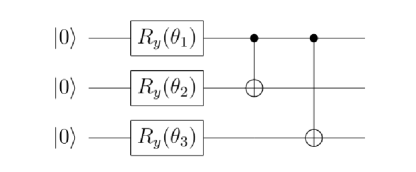
Figure 1: The quantum circuit diagram of the preparation of the initial quantum states.

Without loss of generality, we take $\theta_{1}={\pi}/{4}$, $\theta_{2}={\pi}/{6}$, $\theta_{3}={\pi}/{8}$. Then, we perform quantum simulation on the Wuyuan 2 device to test our constraint relation. We repeat the experiment 5 times and each circuit is implemented in 10000 shots. The set of 4 tomographic measurement operators and the corresponding counts for the qubit A, B or C are respectively shown in Table 1.

• Table 1. Tomographic measurement operators and the corresponding counts for each qubit.

$\mu_{i}$	$n_{i}$	qubit A	qubit B	qubit C
$\mu_{0}=|0\rangle\langle 0|+|1\rangle\langle 1|$	$n_{0}$	5000	5000	5000
$\mu_{1}=|0\rangle\langle 0|$	$n_{1}$	8252	7743	7740
$\mu_{2}=|-\rangle\langle-|$	$n_{2}$	4411	2729	3196
$\mu_{3}=|R\rangle\langle R|$	$n_{3}$	4989	4951	4941

To proceed, we calculate the Stokes parameters. Substituting these results into the formula (22) yields

$$\rho_{A}=\left(\begin{array}[]{cc}0.8252&~{}0.0589-\textrm{i}0.0011\\ 0.0589+\textrm{i}0.0011&~{}0.1748\\ \end{array}\right),$$ (26)

$$\rho_{B}=\left(\begin{array}[]{cc}0.7743&~{}0.2271-\textrm{i}0.0049\\ 0.2271+\textrm{i}0.0049&~{}0.2257\\ \end{array}\right)$$ (29)

and

$$\rho_{C}=\left(\begin{array}[]{cc}0.7740&~{}0.1804-\textrm{i}0.0059\\ 0.1804+\textrm{i}0.0059&~{}0.2260\\ \end{array}\right).$$ (32)

A straightforward calculation shows that these density matrices satisfy the following properties: (i) the normalization, $\textrm{Tr}(\rho_{k})=1$; (ii) the Hermiticity, $\rho^{{\dagger}}_{k}=\rho_{k}$; and (iii) the positive semidefiniteness, the eigenvalues lie in the interval $[0,1]$ and $\textrm{Tr}(\rho^{2}_{k})<1$, where $k=A,B,C$.

Then we calculate the quantities $V_{k}$, $P_{k}$ and $Q$, as shown in Table 2.

• Table 2. Experimental results of $V_{k}$, $P_{k}$ and $Q$.

$V_{A}$	$V_{B}$	$V_{C}$	$P_{A}$	$P_{B}$	$P_{C}$	$Q$
0.1178	0.4543	0.3610	0.6504	0.5486	0.5480	0.5420

By this, one can obtain

$$Q+\frac{1}{3}\sum_{k=A,B,C}V_{k}^{2}+\frac{1}{3}\sum_{k=A,B,C}P_{k}^{2}=1.0003.$$ (33)

The result is very close to the theoretical value 1, given by Eq. (21). It means that, the constraint relation of the entanglement measure, quantitative waviness and particleness can be tested by using the quantum cloud platform.

In order to provide some perspective on how the tripartite entanglement constraint on wave-particle duality, we now consider two cases with a random variable $\theta$, e.g., $\theta_{1}=\theta_{2}=\theta_{3}=\theta$ and $\theta_{1}=\theta$, $\theta_{2}=\theta_{3}=0$ in the state (23).

Theoretically, for $\theta_{1}=\theta_{2}=\theta_{3}=\theta$ one gets

$$\frac{1}{3}\sum_{k=A,B,C}V_{k}^{2}=\frac{1}{3}(\sin^{6}\theta+2\sin^{2}\theta),$$ (34)

$$\frac{1}{3}\sum_{k=A,B,C}P_{k}^{2}=\frac{1}{3}(2\cos^{4}\theta+\cos^{2}\theta),$$ (35)

$$Q=-\frac{1}{3}(\sin^{6}\theta+2\sin^{4}\theta-3\sin^{2}\theta);$$ (36)

and for $\theta_{2}=\theta_{3}=0$, $\theta_{1}=\theta$ we have

$$\frac{1}{3}\sum_{k=A,B,C}V_{k}^{2}=0,$$ (37)

$$\frac{1}{3}\sum_{k=A,B,C}P_{k}^{2}=\cos^{2}\theta,$$ (38)

$$Q=\sin^{2}\theta.$$ (39)

Taking $\theta=0,\pi/4,\pi/2,3\pi/4,\pi$, respectively, we perform quantum simulation on the Wuyuan 2 device. Finally, we calculate each quantity on the left hand side of the Eq. (21), as shown in Table 3 for $\theta_{1}=\theta_{2}=\theta_{3}=\theta$ and Table 4 for $\theta_{1}=\theta$, $\theta_{2}=\theta_{3}=0$.

• Table 3. Experimental results for $\theta_{1}=\theta_{2}=\theta_{3}=\theta$.

$\theta$	$\frac{1}{3}\Sigma_{k=A,B,C}V_{k}^{2}$	$\frac{1}{3}\Sigma_{k=A,B,C}P_{k}^{2}$	$Q$	sum
0	0.0001	0.8960	0.1030	0.9991
$\frac{\pi}{4}$	0.3322	0.2910	0.3770	1.0002
$\frac{\pi}{2}$	0.8670	0.0001	0.1330	1.0001
$\frac{3\pi}{4}$	0.3320	0.2930	0.3750	1.0000
$\pi$	0.0001	0.8680	0.1370	1.0051

• Table 4. Experimental results for $\theta_{1}=\theta$, $\theta_{2}=\theta_{3}=0$.

$\theta$	$\frac{1}{3}\Sigma_{k=A,B,C}V_{k}^{2}$	$\frac{1}{3}\Sigma_{k=A,B,C}P_{k}^{2}$	$Q$	sum
0	0.0001	0.9000	0.0990	0.9991
$\frac{\pi}{4}$	0.0002	0.4430	0.5570	1.0002
$\frac{\pi}{2}$	0.0002	0.0001	0.9997	1.0000
$\frac{3\pi}{4}$	0.0002	0.4430	0.5570	1.0002
$\pi$	0.0002	0.8810	0.1190	1.0002

As shown in Figs. 2 and 3, furthermore, we show the experimental test as well as the theoretical results, for these two cases, respectively. The solid lines are the theoretical results to fit the experimentally achieved visibility and the experimental data are respectively taken to $\theta=0,\pi/4,\pi/2,3\pi/4,\pi$. As a result, it can be found that these experimental outcomes are almost identical with the theoretical values. The difference between the experimental and theoretical results are mainly caused by the qubit crosstalk, CNOT gates in quantum circuit and readout errors, etc. It is worth mentioning that the constraint of the Eq. (21) on their variation is very strong, since the sums of these three quantities (quantitative waviness, particleness and the global entanglement) are always taken to 1.

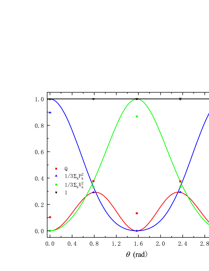
Figure 2: Theoretical results versus experimental tests for cases $\theta_{1}=\theta_{2}=\theta_{3}=\theta$.

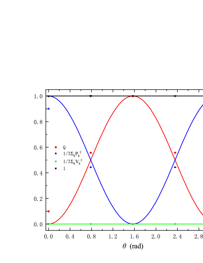
Figure 3: Theoretical results versus experimental tests for cases $\theta_{1}=\theta$, $\theta_{2}=\theta_{3}=0$.

5 Discussion and summary

In summary, we have proposed a constraint relation involving the global tripartite entanglement measure and quantitative wave-particle duality for the tripartite systems. In terms of quantum state tomography, we have performed quantum simulation to test the constraint relation on the Wuyuan 2 superconducting quantum device. It is found that the results of experimental test are almost identical with the theoretical values. This means that the quantitative waviness and particleness are closely related to the global entanglement in quantum system.

Declarations

Data availability statement

The authors confirm that the data supporting the findings of this study are available within the article.

Funding and/or Conflicts of interests/Competing interests

The authors declare that they have no conflicts of and competing interests.

References

- (1) De Broglie, L.: Recherches sur la theorie des quanta, Thesis (Paris), (1924), Research on the theory of quanta. Annals of Physics 3, 22 (1925)
- (2) Bohr, N.: The quantum postulate and the recent development of atomic theory. Nature (London) 121, 580-590 (1928)
- (3) Heisenberg, W.: Über quantentheoretische Umdeutung kinematischer und mechanischer Beziehungen. Z. Phys. 33, 879-893 (1925)
- (4) Wootters, W. K., Zurek, W. H.: Complementarity in the double-slit experiment: quantum nonseparability and a quantitative statement of Bohr’s principle. Phys. Rev. D 19, 473-484 (1979)
- (5) Greenberger, D. M., Yasin, A.: Simultaneous wave and particle knowledge in a neutron interferometer. Phys. Lett. A 128, 391-394 (1988)
- (6) Englert, B.-G.: Fringe visibility and which-way information: an inequality. Phys. Rev. Lett. 77, 2154-2157 (1996)
- (7) Vaccaro, J. A.: Particle-wave duality: a dichotomy between symmetry and asymmetry. Proc. R. Soc. A 468, 1065-1084 (2012)
- (8) Menon, K. K., Qureshi, T.: Wave-particle duality in asymmetric beam interference. Phys. Rev. A 98, 022130 (2018)
- (9) Dürr, S.: Quantitative wave-particle duality in multibeam interferometers. Phys. Rev. A 64, 042113 (2001)
- (10) Englert, B.-G., Kaszlikowski, D., Kwek, L. C., Chee, W. H.: Wave-particle duality in multi-path interferometers: general concepts and three-path interferometers. Int. J. Quant. Inf. 6, 129-157 (2008)
- (11) Bera, M. N., Qureshi, T., Siddiqui, M. A., Pati, A. K.: Duality of quantum coherence and path distinguishability. Phys. Rev. A 92, 012118 (2015)
- (12) Coles, P. J.: Entropic framework for wave-particle duality in multipath interferometers. Phys. Rev. A 93, 062111 (2016)
- (13) Jaeger, G., Horne, M. A., Shimony, A.: Complementarity of one-particle and two-particle interference. Phys. Rev. A 48, 1023 (1993)
- (14) Jaeger, G., Shimony, A., Vaidman, L.: Two interferometric complementarities. Phys. Rev. A 51, 54 (1995)
- (15) Jakob, M., Bergou, J. A.: Quantitative complementarity relations in bipartite systems: entanglement as a physical reality. Opt. Commun. 283, 827-830 (2010)
- (16) Jakob, M., Bergou, J. A.: Complementarity and entanglement in bipartite qudit systems. Phys. Rev. A 76, 052107 (2007)
- (17) Schwaller, N., Dupertuis, M.-A., Javerzac-Galy, C.: Evidence of the entanglement constraint on wave-particle duality using the IBM Q quantum computer. Phys. Rev. A 103, 022409 (2021)
- (18) Qureshi, T.: Predictability, distinguishability, and entanglement. Opt. Lett. 46, 492-495 (2021)
- (19) Marrou, J. P., La Torre, C. M., Jara, M., De Zela, F.: Wave-particle duality in tripartite systems. J. Opt. Soc. Am. A 40(4), c22-c29 (2023)
- (20) Meyer, D. A., Wallach, N. R.: Global entanglement in multiparticle systems. J. Math. Phys. 43, 4273-4278 (2002)
- (21) Brennen, G. K.: An observable measure of entanglement for pure states of multi-qubit systems. Quantum Inf. Comput. 3, 619-626 (2003)
- (22) James, D. F. V., Kwiat, P. G., Munro, W. J., White, A. G.: Measurement of qubits. Phys. Rev. A 64, 052312. (2001)
- (23) OriginQ Quantum Experience, https://qcloud.originqc.com.cn/.