Anytime Solvers for Variational Inequalities:
the (Recursive) Safe Monotone Flows

Abstract

This paper synthesizes anytime algorithms, in the form of continuous-time dynamical systems, to solve monotone variational inequalities. We introduce three algorithms that solve this problem: the projected monotone flow, the safe monotone flow, and the recursive safe monotone flow. The first two systems admit dual interpretations: either as projected dynamical systems or as dynamical systems controlled with a feedback controller synthesized using techniques from safety-critical control. The third flow bypasses the need to solve quadratic programs along the trajectories by incorporating a dynamics whose equilibria precisely correspond to such solutions, and interconnecting the dynamical systems on different time scales. We perform a thorough analysis of the dynamical properties of all three systems. For the safe monotone flow, we show that equilibria correspond exactly with critical points of the original problem, and the constraint set is forward invariant and asymptotically stable. The additional assumption of convexity and monotonicity allows us to derive global stability guarantees, as well as establish the system is contracting when the constraint set is polyhedral. For the recursive safe monotone flow, we use tools from singular perturbation theory for contracting systems to show KKT points are locally exponentially stable and globally attracting, and obtain practical safety guarantees. We illustrate the performance of the flows on a two-player game example and also demonstrate the versatility for interconnection and regulation of dynamical processes of the safe monotone flow in an example of a receding horizon linear quadratic dynamic game.

,

1 Introduction

Variational inequalities encompass a wide range of problems arising in operations research and engineering applications, including minimizing a function, characterizing Nash equilibria of a game, and seeking saddle points of a function. In this paper, we synthesize continuous-time flows whose trajectories converge to the solution set of a monotone variational inequality while respecting the constraints at all times.

Our motivation for considering this problem is two-fold. First, iterative algorithms in numerical computing can be interpreted as dynamical systems. This opens the door for the use of controls and system-theoretic tools to characterize their qualitative and quantitative properties, e.g., stability of solutions, convergence rate, and robustness to disturbances. In turn, the availability of such characterization sets the stage for developing sample-data implementations and systematically designing new algorithms equipped with desired properties.

The second motivation stems from problems where the solution to the variational inequality is used to regulate a physical process modeled as a dynamically evolving plant (e.g., providing setpoints, specifying optimization-based controllers, steering the plant toward an optimal steady-state). This type of problem arises in multiple application areas, including power systems, network congestion control, and traffic networks. In these settings, the algorithm used to solve the variational inequality is interconnected with a plant, and thus the resulting coupled system naturally lends itself to system-theoretic analysis and design. We are particularly interested in situations where the problem incorporates constraints which, when violated, would threaten the safe operation of the physical system. In such cases, it is desirable that the algorithm is anytime, meaning that it is guaranteed to return a feasible point even when terminated before it has converged to a solution. The anytime property ensures that the specifications conveyed to the plant remain feasible at all times.

Related Work

The study of the interplay between continuous-time dynamical systems and variational inequalities has a rich history. In the context of optimization, classical references include [7, 16, 31]. For general variational inequalities, flows solving them can be obtained through differential inclusions involving monotone set-valued maps, originally introduced in [15]. These systems have been equivalently described as a projected dynamical systems [36] and complementarity systems [17, 30]. One limitation of these systems is that they are, in general, discontinuous, which poses challenges both for their theoretical analysis and practical implementation.

The interconnection of optimization algorithms with physical plants has attracted much attention recently [20, 29]. The specific setting where the algorithm optimizes the steady-state of the plant is typically referred to as online feedback optimization and has been studied in the context of power systems [23, 33], network congestion control [35], and traffic networks [11], to name a few. Recently this framework has also been generalized to game scenarios [1, 10]. A complementary approach uses extremum seeking control [6], which has been generalized to the setting of games in [28]. Extremum seeking differs from the methods introduced here in that they are typically zeroth-order methods, and do not offer exact stability guarantees. The recent work [43] considers safety guarantees for extremum seeking control for the special case of a single inequality constraint. In fact, the proposed algorithm can be understood as an approximation of the safe gradient flow in [3], which is a precursor for constrained optimization of the algorithms proposed here for constraint sets parameterized by multiple inequality and equalities.

To synthesize our flows, we employ techniques from safety-critical control [4, 19], which refers to the problem of designing a feedback controller that ensures that the state of the system satisfies certain constraints. The problem of ensuring safety is typically formalized by specifying a set of states where the system is said to remain safe, and ensuring the safe set is forward invariant. The work [12] reviews set invariance in control. A popular technique for synthesizing safe controllers uses the concept of control barrier functions (CBFs), see [42, 5, 44] and references therein, to specify optimization-based feedback controllers which “filter” a nominal system to ensure it remains in the safe set. Here, we apply this strategy to synthesize anytime algorithms, viewing the constraint set as a safety set and the monotone operator of the variational inequality as the nominal system. This view has connections to projected dynamical systems, whose relationship with CBF-based control design has recently been explored in [25], and leads to the alternative “projection-based” interpretation of the projected monotone flow and safe monotone flow proposed here.

Statement of Contributions

We consider the synthesis of continuous-time dynamical systems solving variational inequalities while respecting the constraints at all times, with a view toward applications where the flow is used to regulate a physical process through interconnection with a dynamically evolving plant. We discuss three flows that solve this problem. The projected monotone flow is already known, but we provide a novel control-theoretic interpretation as a control system whose closed-loop behavior is as close as possible to the monotone operator while still belonging to the tangent cone of the constraint set. The safe monotone flow can be interpreted either as a control system with a feedback controller synthesized using techniques from safety-critical control or as an approximation of the projected monotone flow. The latter interpretation relies on the novel notion of restricted tangent set, which generalizes the usual concept of tangent cone from variational geometry. We show that equilibria correspond exactly with critical points of the original problem, establish existence and uniqueness of solutions, and characterize the regularity properties of flow. We also show that the constraint set is forward invariant and asymptotically stable, and derive global stability guarantees under the additional assumption of convexity and monotonicity. Our technical analysis relies on a suite of Lyapunov functions to establish stability properties with respect to the constraint set and the whole state space. When the constraint set is polyhedral, we establish that the system is contracting and exponentially stable. Finally, the recursive safe monotone flow bypasses the need for continuously solving quadratic programs along the trajectories by incorporating a dynamics whose equilibria precisely correspond to such solutions, and interconnecting the dynamical systems on different time scales. Using tools from singular perturbation theory for contracting systems, we show that for variational inequalities with polyhedral constraints, the KKT points are locally exponentially stable and globally attracting, and obtain practical safety guarantees. We compare the three flows on a simple two-player game and also demonstrate how the safe monotone flow can be interconnected with dynamical processes on an example of a receding horizon linear quadratic dynamic game.

The algorithms introduced here generalize the safe gradient flow introduced in our previous work [3]. With respect to it, our treatment extends the results in three key ways. First, we consider variational inequalities, rather than just constrained optimization problems, making the flows introduced here applicable to a much broader range of problems. Second, with assumptions of monotonicity and convexity of the constraints, we obtain global stability and convergence results, rather than local stability results. Third, the rigorous characterization of the contractivity properties of the safe monotone flow paves the way for its interconnection with other dynamically evolving processes. In fact, the proposed recursive safe monotone flow critically builds on this analysis by leveraging different timescales and singular perturbation theory.

2 Preliminaries

We review here basic notions from variational inequalities, projections, and set invariance. Readers familiar with these concepts can safely skip this section.

2.1 Notation

Let denote the set of real numbers. For $c\in$, $[c]_{+}=\max\{0,c\}$. For $x\in^{n}$, $x_{i}$ denotes the $i$th component and $x_{-i}$ denotes all components of $x$ excluding $i$. For $v,w\in^{n}$, $v\leq w$ (resp. $v<w$) denotes $v_{i}\leq w_{i}$ (resp. $v_{i}<w_{i}$) for $i\in\{1,\dots,n\}$. We let $\left\lVert v\right\rVert$ denote the Euclidean norm. We write $Q\succeq 0$ (resp., $Q\succ 0$) to denote $Q$ is positive semidefinite (resp., $Q$ is positive definite). Given $Q\succeq 0$, we let $\left\lVert x\right\rVert_{Q}=\sqrt{x^{\top}Qx}$. For a symmetric $Q$, $\lambda_{\text{min}}(Q)$ and $\lambda_{\textnormal{max}}{(Q)}$ denote the minimum and maximum eigenvalues of $Q$, resp. Given $C\subset^{n}$, the distance of $x\in^{n}$ to $C$ is $\textnormal{dist}(x,C)=\inf_{y\in C}\left\lVert x-y\right\rVert$. We let $\overline{C}$, $\text{int}(C)$, and $\partial C$ denote its closure, interior, and boundary, resp. The projection map onto $\overline{\mathcal{C}}$ is $\Pi_{\mathcal{C}}:^{n}\rightrightarrows\overline{\mathcal{C}}$, where $\Pi_{\mathcal{C}}(x)=\big{\{}y\in\overline{\mathcal{C}}\mid\left\lVert x-y\right\rVert=\textnormal{dist}(x,\mathcal{C})\big{\}}$. Given a closed and convex set $\mathcal{C}\subset^{n}$, the normal cone to $\mathcal{C}$ at $x\in^{n}$ is $N_{\mathcal{C}}(x)=\{d\in^{n}\mid d^{\top}(x^{\prime}-x)\leq 0,\;\forall x^{\prime}\in\mathcal{C}\}$ and the tangent cone to $\mathcal{C}$ at $x$ is $T_{\mathcal{C}}(x)=\{\xi\in^{n}\mid d^{\top}\xi\leq 0,\;\forall d\in N_{\mathcal{C}}(x)\}$.

Given $g:^{n}\to$, we denote its gradient by $\nabla g$. For $g:^{n}\to^{m}$, $\frac{\partial g(x)}{\partial x}$ denotes its Jacobian. For $I\subset\{1,2,\dots,m\}$, we denote by $\frac{\partial g_{I}(x)}{\partial x}$ the matrix whose rows are $\{\nabla g_{i}(x)^{\top}\}_{i\in I}$. Given a function $f:^{n}\to$, we say it is directionally differentiable if for all $\xi\in^{n}$, the following limit exists

$$f^{\prime}(x;\xi)=\lim_{h\to 0^{+}}\frac{f(x+h\xi)-f(x)}{h}.$$

Given a vector field $\mathcal{G}:^{n}\to^{n}$ and a function $V:^{n}\to$, the Upper-right Dini derivative of $V$ along $\mathcal{G}$ is

$$D^{+}_{\mathcal{G}}V(x)=\limsup_{h\to 0^{+}}\frac{1}{h}\left(V(\Phi_{h}(x))-V(x)\right),$$

where $\Phi_{h}$ is the flow map corresponding to $\dot{x}=\mathcal{G}(x)$. When $V$ is directionally differentiable $D^{+}_{\mathcal{G}}V(x)=V^{\prime}(x,\mathcal{G}(x))$ and when $V$ is differentiable, then $D^{+}_{\mathcal{G}}V(x)=\nabla V(x)^{\top}\mathcal{G}(x)$.

2.2 Variational Inequalities

Here we review the basic theory of variational inequalities following [27]. Let $F:^{n}\to^{n}$ be a map and $\mathcal{C}\subset^{n}$ a set of constraints. A variational inequality refers to the problem of finding $x^{*}\in\mathcal{C}$ such that

$$(x-x^{*})^{\top}F(x^{*})\geq 0,\qquad\forall x\in\mathcal{C}.$$ (1)

We use $\textnormal{VI}(F,\mathcal{C})$ to refer to the problem (1) and $\textnormal{SOL}(F,\mathcal{C})$ to denote its set of solutions. Variational inequalities provide a framework to study many different analysis and optimization problems, including

• Solving the nonlinear equation $F(x^{*})=0$, which corresponds to $\textnormal{VI}(F,^{n})$;

• Minimizing the function $f:^{n}\to$ subject to the constraint that $x\in\mathcal{C}$, which corresponds to $\textnormal{VI}(\nabla f,\mathcal{C})$;

• Finding saddle points of the function $\ell:^{n}\times^{m}\to$ subject to the constraints that $x_{1}\in X_{1}$ and $x_{2}\in X_{2}$, which corresponds to $\textnormal{VI}([\nabla_{x_{1}}\ell;-\nabla_{x_{2}}\ell],X_{1}\times X_{2})$.

• Finding the Nash equilibria of a game with $N$ agents, where the $i$th agent wants to minimize the cost $J_{i}(x_{i},x_{-i})$ subject to the constraint $x_{i}\in X_{i}$, which corresponds to $\textnormal{VI}(F,\mathcal{C})$, where $F$ is the pseudogradient operator defined by $F(x)=(\nabla_{x_{1}}J_{1}(x),\dots,\nabla_{x_{N}}J_{N}(x))$ and $\mathcal{C}=X_{1}\times X_{2}\times\cdots\times X_{N}$.

The map $F:^{n}\to^{n}$ is monotone if

$$(x_{1}-x_{2})^{\top}(F(x_{1})-F(x_{2}))\geq 0,$$

for all $x_{1},x_{2}\in^{n}$, and $F$ is $\mu$-strongly monotone if there exists $\mu>0$ such that

$$(x_{1}-x_{2})^{\top}(F(x_{1})-F(x_{2}))\geq\mu\left\lVert x_{1}-x_{2}\right\rVert^{2},$$

for all $x_{1},x_{2}\in^{n}$. When $F$ is a gradient map, i.e. $F=\nabla f$ for some function $f:^{n}\to$, then monotonicity (resp. $\mu$-strong monotonicity) is equivalent to convexity (resp. strong convexity) of $f$. When $F$ is monotone and $\mathcal{C}$ is convex, $\textnormal{VI}(F,\mathcal{C})$ is a monotone variational inequality.

In order to provide a characterization of the solution set $\textnormal{SOL}(F,\mathcal{C})$, we need to introduce a more explicit description of the set of constraints. Suppose that $g:^{n}\to^{m}$ and $h:^{n}\to^{k}$ are continuously differentiable and $\mathcal{C}$ is described by inequality constraints and affine equality constraints,

$$\mathcal{C}=\{x\in^{n}\mid g(x)\leq 0,\;h(x)=Hx-c_{h}=0\},$$ (2)

where $A\in^{k\times n}$ and $b\in^{k}$. For $x\in^{n}$, we denote the active constraint, inactive constraint, and constraint violation sets, resp., as

$$I_{0}(x) =\{i\in[1,m]\mid g_{i}(x)=0\},$$

$$I_{-}(x) =\{i\in[1,m]\mid g_{i}(x)<0\},$$

$$I_{+}(x) =\{i\in[1,m]\mid g_{i}(x)>0\}.$$

The problem (1) satisfies the constant-rank condition at $x\in\mathcal{C}$ if there exists an open set $U$ containing $x$ such that for all $I\subset I_{0}(x)$, the rank of $\{\nabla g_{i}(y)\}_{i\in I}\cup\{\nabla h_{j}(y)\}_{j=1}^{k}$ remains constant for all $y\in U$. The problem (1) satisfies the Mangasarian-Fromovitz Constraint Qualification (MFCQ) condition at $x\in\mathcal{C}$ if $\{\nabla h_{j}(x)\}_{i=1}^{k}$ are linearly independent, and there exists $\xi\in^{n}$ such that $\nabla g_{i}(x)^{\top}\xi<0$ for all $i\in I_{0}(x)$, and $\nabla h_{j}(x)^{\top}\xi=0$ for all $j\in\{1,\dots,k\}$. If MFCQ holds at $x^{*}\in\mathcal{C}$, then, if $x^{*}$ satisfies (1), there exists $(u^{*},v^{*})\in^{m}\times^{k}$ such that

$$F(x^{*})+\sum_{i=1}^{m}u^{*}_{i}\nabla g_{i}(x^{*})+\sum_{j=1}^{k}v_{j}^{*}\nabla h_{j}(x^{*}) =0$$ (3a)

$$g(x^{*}) \leq 0$$ (3b)

$$h(x^{*}) =0$$ (3c)

$$u^{*} \geq 0$$ (3d)

$$(u^{*})^{\top}g(x^{*}) =0.$$ (3e)

Equations (3) are called the KKT conditions. A point $(x^{*},u^{*},v^{*})$ satisfying them is a KKT triple and the pair $(u^{*},v^{*})$ is a Lagrange multiplier. We denote the set of KKT triples by $\textnormal{KKT}(F,\mathcal{C})$. For monotone variational inequalities, when MFCQ holds at $x^{*}$, then the KKT conditions are both necessary and sufficient for $x^{*}\in\textnormal{SOL}(F,\mathcal{C})$. When $F$ is monotone $\textnormal{SOL}(F,\mathcal{C})$ is closed and convex. If $F$ is additionally $\mu$-strongly monotone, then the set of solutions is a singleton.

2.3 Controller Synthesis for Set Invariance

We review here notions from the theory of set invariance for control systems following [12] and discuss methods for synthesizing feedback controllers that ensure it. Consider a control-affine system

$$\dot{x} =\mathcal{F}(x,\mu)=F_{0}(x)+\sum_{i=1}^{r}\mu_{i}F_{i}(x),$$ (4)

with Lipschitz-continuous vector fields $F_{i}:^{n}\to^{n}$, for $i\in\{0,\dots,r\}$, and a set $\mathcal{U}\subset^{m}$ of valid control inputs $\mu$. Let $\mathcal{C}\subset^{n}$ be a constraint set of the form (2) to which we want to restrict the evolution of the system. We consider the problem of designing a feedback controller $k:^{n}\to\mathcal{U}$ such that $\mathcal{C}$ is forward invariant with respect to the closed-loop dynamics $\dot{x}=\mathcal{F}(x,k(x))$. In applications, $\mathcal{C}$ often corresponds to the set of states for which the system can operate safely. For this reason, we refer to $\mathcal{C}$ as the safety set, and call the system safe under a controller $k$ if $\mathcal{C}$ is forward invariant. A controller ensuring safety is safeguarding. We discuss two optimization-based strategies for synthesizing safeguarding controllers.

2.3.1 Safeguarding Control via Projection

The first strategy ensures the closed-loop dynamics lie in the tangent cone of the safety set. If MFCQ holds at $x\in\mathcal{C}$, the tangent cone can conveniently be expressed as, cf. [40, Theorem 6.31], $T_{\mathcal{C}}(x)=\{\xi\in^{n}\left|\frac{\partial h(x)}{\partial x}\xi=0,\frac{\partial g_{I}(x)}{\partial x}\xi\leq 0\right.\}$. We then define the set-valued map $K_{\text{proj}}:^{n}\rightrightarrows\mathcal{U}$ which characterizes the set of inputs that ensure the system remains inside the safety set. The set has the form,

$$K_{\text{proj}}(x) =\big{\{}\mu\in\mathcal{U}\mid$$

$$D^{+}_{F_{0}}g_{i}(x)+\sum_{\ell=1}^{r}\mu_{\ell}D^{+}_{F_{\ell}}g_{i}(x)\leq 0,\;i\in I(x),$$

$$D^{+}_{F_{0}}h_{j}(x)+\sum_{\ell=1}^{r}\mu_{\ell}D^{+}_{F_{\ell}}h_{j}(x)=0,\;j=1,\dots,k\big{\}}.$$

Any feedback $k:\mathcal{C}\to\mathcal{U}$ such that $k(x)\in K_{\text{proj}}(x)$ for $x\in\mathcal{C}$ renders $\mathcal{C}$ forward invariant.

Lemma 2.1.

(Projection-based Safeguarding Feedback) Consider the system (4) with safety set $\mathcal{C}$ and suppose that $K_{\text{proj}}(x)\neq\emptyset$ for all $x\in\mathcal{C}$. Then, the feedback controller $k:\mathcal{C}\to\mathcal{U}$ is safeguarding if $k(x)\in K_{\text{proj}}(x)$ for all $x\in\mathcal{C}$ and the closed-loop system $\dot{x}=\mathcal{F}(x,k(x))$ admits a unique solution for all initial conditions.

By hypothesis, the closed-loop system satisfies $\mathcal{F}(x,k(x))\in T_{\mathcal{C}}(x)$ for all $x\in\mathcal{C}$. Then, $\mathcal{C}$ is forward invariant by Nagumo’s Theorem [12, Theorem 3.1]. ∎

To synthesize a safeguarding controller, we propose a strategy where $k(x)$ at each $x\in\mathcal{C}$ is expressed as the solution to a mathematical program. Because $K_{\text{proj}}(x)$ is defined in terms of affine constraints on the control input $\mu$, we can readily express a feedback satisfying the hypotheses of Lemma 2.1 in the form of a mathematical program,

$$k(x)\in\underset{\mu\in K_{\text{proj}}(x)}{\text{argmin}}J(x,\mu),$$ (5)

for an appropriate choice of cost function $J:\mathcal{C}\times\mathcal{U}\to$. In general, care must be taken to ensure that the set $K_{\text{proj}}$ is nonempty and that the controller $k$ in (5) satisfies appropriate regularity conditions to ensure existence and uniqueness for solutions of the resulting closed-loop dynamics. Even if these properties hold, the approach has several limitations: the controller is ill-defined for initial conditions lying outside the safety set and the closed-loop system in general is nonsmooth.

2.3.2 Safeguarding Control via Control Barrier Functions

The second strategy for synthesizing safeguarding controllers addresses the limitations of projection-based methods. The approach relies on the notion of a vector control barrier functions [4, 3]. Given a set $X\supset\mathcal{C}$ and set of valid control inputs $\mathcal{U}\subset^{m}$, we say the pair $(g,h):^{n}\times^{k}\to^{m}$ is a $(m,k)$-vector control barrier function (VCBF) for $\mathcal{C}$ on $X$ relative to $\mathcal{U}$ if there exists $\alpha>0$ such that the map $K_{\text{cbf},\alpha}:^{n}\rightrightarrows\mathcal{U}$ given by

$$K_{\text{cbf},\alpha}(x) =\big{\{}\mu\in\mathcal{U}\mid$$

$$D^{+}_{F_{0}}g_{i}(x)+\sum_{\ell=1}^{r}\mu_{\ell}D^{+}_{F_{\ell}}g_{i}(x)\!+\!\alpha g_{i}(x)\leq 0,$$

$$D^{+}_{F_{0}}h_{j}(x)+\sum_{\ell=1}^{r}\mu_{\ell}D^{+}_{F_{\ell}}h_{j}(x)+\alpha h_{j}(x)=0,$$

$$\leq i\leq m,\;1\leq j\leq k\big{\}},$$

takes nonempty values for all $x\in X$. Similar to the previous strategy, the set $K_{\text{cbf},\alpha}$ characterizes the set of inputs which ensure that the state remains inside the safe set. Unlike the previous strategy, this assurance is implemented gradually: the parameter $\alpha$ corresponds to how tolerant we are of trajectories approaching the boundary of the safety set, with smaller values of $\alpha$ corresponding to situations where the trajectories beginning in the interior are more aggressively controlled. For $\alpha=\infty$, the set corresponds to $K_{\text{proj}}$.

When $m=1$ and $k=0$, a vector control barrier function is equivalent to the usual notion of a control barrier function [4, Definition 2]. The generalization provided by VCBFs allows us to consider a broader class of safety sets.

Lemma 2.2.

(VCBF-based Safeguarding Feedback) Consider the system (4) with safety set $\mathcal{C}$ and suppose $(g,h)$ is a vector control barrier function for $\mathcal{C}$ on $X$ relative to $\mathcal{U}$. Then, the feedback controller $k:X\to\mathcal{U}$ is safeguarding and ensures asymptotic stability of $\mathcal{C}$ on $X$ if $k(x)\in K_{\alpha}(x)$ for all $x\in X$ and the closed-loop system $\dot{x}=\mathcal{F}(x,k(x))$ admits a unique solution for all initial conditions.

To synthesize a safeguarding feedback controller, one can pursue a design using a similar approach to Section 2.3.1. Given a cost function $J:X\times\mathcal{U}\to$, we let $k(x)$ solve the following mathematical program:

$$k(x)\in\underset{\mu\in K_{\text{cbf},\alpha}(x)}{\text{argmin}}J(x,\mu).$$ (6)

Similarly to the case of projection-based safeguarding feedback control, care must be taken to verify the existence and uniqueness of solutions to the closed-loop system, as well as to handle situations where (6) does not have unique solutions. If these properties hold, then the control design addresses the challenges of projection-based methods. In particular, we can ensure that a controller of the form (6) is well-defined outside the safety set and results in closed-loop system with continuous solutions, under mild conditions which we discuss in the following sections.

3 Problem Formulation

Consider a variational inequality $\textnormal{VI}(F,\mathcal{C})$ defined by a continuously differentiable map $F:^{n}\to^{n}$ and a convex set $\mathcal{C}$ of the form (2), where $g:^{n}\to^{m}$ is continuously differentiable. Our goal is to synthesize a dynamical system that solves the variational inequality. We formalize this next.

Problem 1.

(Anytime solver of variational inequality) Design a dynamical system, $\dot{x}=\mathcal{G}(x)$, which is well defined on a set $X$ containing $\mathcal{C}$ such that

1. Trajectories of the system converge to $\textnormal{SOL}(F,\mathcal{C})$;

2. $\mathcal{C}$ is forward invariant;

3. Trajectories of the system with initial condition outside $\mathcal{C}$ converge to $\mathcal{C}$.

Item (i) ensures that the dynamical system can be viewed as an algorithm which solves (1): solutions can be obtained by simulating system trajectories and taking the limit as $t\to\infty$ of $x(t)$. Item (ii) ensures that this algorithm is anytime, meaning that even if terminated early, it is guaranteed to return a feasible solution provided the initial condition is feasible. Item (iii) accounts for infeasible initial conditions, and ensures asymptotic safety. Both the expression of the algorithm in the form of a continuous-time dynamical system and the anytime property are particularly useful for real-time applications, where the algorithm might be interconnected with other physical processes – e.g., when the algorithm output is used to regulate a physical plant and constraints of the optimization problem ensure the safe operation of the plant.

In the following, we introduce three dynamics to solve Problem 1. The first, synthesized using the technique outlined in Section 2.3.1, is the projected monotone flow. This dynamics is already well-known but we reinterpret it here through the lens of control theory. The next two, synthesized using the technique outlined in Section 2.3.2, are the safe monotone flow and the recursive safe monotone flow. Both dynamics are entirely novel.

4 Projected Monotone Flow

In this section, we discuss our first solution to Problem 1, in the form of the projected monotone flow. We show that the system can be implemented in two equivalent ways: either as a control system with a feedback controller designed using the strategy outlined in Section 2.3.1, or as a projected dynamical system. In fact, this system admits many other equivalent descriptions, for example in terms of monotone differential inclusions, or complementarity systems [17, 30, 8], and its properties have been extensively studied [36]. However, we focus here on the control-based and projection-based forms. In the following sections we describe in detail the derivation of each implementation, show they are equivalent, and discuss the properties of the resulting flow regarding safety and stability.

4.1 Control-Based Implementation

Our design strategy originates from the observation that, when $F$ is monotone, the system $\dot{x}=-F(x)$ finds solutions to the unconstrained variational inequality $\textnormal{VI}(F,^{n})$. However, trajectories flowing along this dynamics might leave the constraint set $\mathcal{C}$. This leads us to consider the control-affine system:

$$\dot{x} =\mathcal{F}(x,u,v)$$ (7)

$$=-F(x)-\sum_{i=1}^{m}u_{i}\nabla g_{i}(x)-\sum_{j=1}^{k}v_{j}\nabla h_{j}(x).$$

Here, we have augmented the system with inputs from the admissible set $\mathcal{U}=^{m}_{\geq 0}\times^{k}$ to modify the flow of the original drift $-F$ to account for the constraints in a way that ensures that the solutions to (7) stay inside of or approach $\mathcal{C}$. The idea is that if the constraint $g_{i}(x)\leq 0$ is in danger of being violated, the corresponding input $u_{i}$ can be increased to ensure trajectories continue to satisfy it. Likewise, the input $v_{j}$ can be increased or decreased to ensure the corresponding constraint $h_{j}(x)=0$ is satisfied along trajectories.

Our design proceeds by thinking of $\mathcal{C}$ as a safety set for the system and using the approach outlined in Section 2.3.1 to synthesize a safeguarding feedback controller $u=k(x)$. Assuming that MFCQ holds for all $x\in\mathcal{C}$, $K_{\text{proj}}:^{n}\rightrightarrows^{m}_{\geq 0}\times^{k}$ takes the form

$$K_{\text{proj}}(x) =\Big{\{}(u,v)\in^{m}_{\geq 0}\times^{k}\mid$$

$$-\frac{\partial g_{I}}{\partial x}F(x)-\frac{\partial g_{I}}{\partial x}\frac{\partial g}{\partial x}^{\top}u-\frac{\partial g_{I}}{\partial x}\frac{\partial h}{\partial x}^{\top}v\leq 0,$$

$$-\frac{\partial h}{\partial x}F(x)-\frac{\partial h}{\partial x}\frac{\partial g}{\partial x}^{\top}u-\frac{\partial h}{\partial x}\frac{\partial h}{\partial x}^{\top}v=0\Big{\}}.$$ (8)

The following result states that the set of admissible controls is nonempty. We omit its proof for space reasons, but note that it readily follows from Farka’s Lemma [39].

Lemma 4.1.

(Projection onto Tangent Cone is Feasible) If $x\in\mathcal{C}$ and MFCQ holds at $x$, then $K_{\text{proj}}(x)\neq\emptyset$.

We then use the feedback controller

$$k(x)\in\underset{(u,v)\in K_{\text{proj}}(x)}{\text{argmin}}J(x,u,v),$$ (9)

where we set the objective function to be

$$J(x,u,v)=\frac{1}{2}\big{\|}\sum_{i=1}^{m}u_{i}\nabla g_{i}(x)+\sum_{j=1}^{k}v_{j}\nabla h_{j}(x)\big{\|}^{2}.$$ (10)

This function measures the magnitude of the “modification” of the drift term in (7). Thus, the QP-based controller (9) has the interpretation, at each $x$, of finding the control input such that the closed-loop system dynamics are as close as possible to $-F(x)$, while still being in $T_{\mathcal{C}}(x)$. In general, the program given by (9) does not have unique solutions. Despite this, we show below that the closed-loop dynamics of (7) is well defined regardless of which solution to (5) is chosen. We refer to it as the projected monotone flow and denote it by $\mathcal{P}$.

4.2 Projection-Based Implementation

The second implementation of the projected monotone flow consists of projecting $-F(x)$ onto the tangent cone of the constraint set. In general, the tangent cone does not have a representation that allows us to compute the projection easily. However, when the appropriate constraint qualification condition holds, the tangent cone admits a convenient parameterization which allows for the projection to be implemented as a quadratic program. Let $x\in\mathcal{C}$ and suppose that MFCQ holds at $x$. It follows that the tangent cone can be parameterized as

$$T_{\mathcal{C}}(x)=\Big{\{}\xi\in^{n}\left|\frac{\partial h(x)}{\partial x}\xi=0,\frac{\partial g_{I_{0}}(x)}{\partial x}\xi\leq 0\right.\Big{\}}.$$ (11)

The projection-based implementation of the projected monotone flow takes then the following form:

$$\dot{x} =\Pi_{T_{\mathcal{C}}(x)}(-F(x))$$ (12)

$$=\underset{\xi\in^{n}}{\text{argmin}}\quad\frac{1}{2}\left\lVert\xi+F(x)\right\rVert^{2}$$

$$\quad\;\text{subject to}\quad\frac{\partial g_{I_{0}}(x)}{\partial x}\xi\leq 0,\frac{\partial h(x)}{\partial x}\xi=0.$$

The projection onto the tangent ensures by Nagumo’s Theorem [12, Theorem 3.1] that $\mathcal{C}$ is forward invariant.

4.3 Properties of Projected Monotone Flow

Here, we lay out the properties of the projected monotone flow. We begin by establishing the equivalence between the control- and projection-based implementations. We then discuss existence and uniqueness of solutions, and finally the stability and safety properties of the dynamics.

4.3.1 Equivalence of Control-Based and Projection-Based Implementations

Equivalence follows directly from the properties of the tangent cone, as we show next.

Proposition 4.2.

(Equivalence of Control-Based and Projected-Based Implementations) Assume MFCQ holds at $x\in\mathcal{C}$ and let $(u,v)$ be any solution to (9) (note that $\mathcal{P}(x)=\mathcal{F}(x,u,v)$). Then, $\mathcal{P}(x)=\Pi_{T_{\mathcal{C}}(x)}(-F(x))$.

Let $(u,v)$ be any solution to (9) and $\xi=\Pi_{T_{\mathcal{C}}(x)}(-F(x))$. Then $\mathcal{F}(x,u,v)\in T_{\mathcal{C}}(x)$, so it follows immediately by optimality of $\xi$ that

$$\left\lVert\xi+F(x)\right\rVert^{2}\leq\left\lVert\mathcal{F}(x,u,v)+F(x)\right\rVert^{2}.$$

Next, because $\xi$ is given by a projection, there exists $w\in N_{\mathcal{C}}(x)$ such that $\xi+F(x)+w=0$, see e.g., [17, Corollary 2]. If MFCQ holds at $x\in\mathcal{C}$, by [40, Theorem 6.14], there exists $(\bar{u},\bar{v})$ such that $w$ can be written as

$$w=\sum_{i=1}^{m}\bar{u}_{i}\nabla g_{i}(x)+\sum_{j=1}^{k}\bar{v}_{j}\nabla h_{j}(x),$$

$$\bar{u}\geq 0,\quad\bar{u}^{\top}g(x)=0.$$

Combining this expression with the fact that $\xi=-F(x)-w\in T_{\mathcal{C}}(x)$ and using the parameterization of the tangent cone in (11), we deduce that $(\bar{u},\bar{v})\in K_{\text{proj}}(x)$. By optimality of $(u,v)$,

$$\left\lVert\xi+F(x)\right\rVert^{2} =\big{\|}\sum_{i=1}^{m}\bar{u}_{i}\nabla g_{i}(x)+\sum_{j=1}^{k}\bar{v}_{j}\nabla h_{j}(x)\big{\|}^{2}$$

$$\geq\big{\|}\sum_{i=1}^{m}u_{i}\nabla g_{i}(x)+\sum_{j=1}^{k}v_{j}\nabla h_{j}(x)\big{\|}^{2}$$

$$=\left\lVert\mathcal{F}(x,u,v)+F(x)\right\rVert^{2}.$$

But since the projection onto the tangent cone must be unique, we conclude $\xi=\mathcal{F}(x,u,v)$. ∎

The value of Proposition 4.2 stems from showing that safety-critical control can be used to systematically design algorithms that solve variational inequalities. Though the control strategy pursued in Section 4.1 results in a known flow, this sets up the basis for employing other design strategies from safety-critical control to yield novel methods, as we will show later.

4.3.2 Existence and Uniqueness of Solutions

The projected monotone flow is discontinuous, and hence one must consider notions of solutions beyond the classical ones, see e.g., [21]. Here, we consider Carathéodory solutions, which are absolutely continuous functions that satisfy (12) almost everywhere. The existence and uniqueness of solutions for all initial conditions follows readily from [8, Chapter 3.2, Theorem 1(i)].

4.3.3 Safety and Stability of Projected Monotone Flow

We now show that the projected monotone flow is safe, meaning that the constraint set $\mathcal{C}$ is forward invariant, and the solution set $\textnormal{SOL}(F,\mathcal{C})$ is stable. Forward invariance of $\mathcal{C}$ follows directly from Nagumo’s Theorem. The equilibria of the projected monotone flow correspond to solutions to $\textnormal{VI}(F,\mathcal{C})$. Finally, stability of a solution $x^{*}$ can be certified using the Lyapunov function $V(x)=\frac{1}{2}\left\lVert x-x^{*}\right\rVert^{2}$, as a consequence of [8, Chapter 3.2, Theorem 1(ii)]. These properties are summarized in the following result.

Theorem 4.3.

(Safe and Stability Properties of Projected Monotone Flow) Let $\mathcal{C}$ be convex and suppose MFCQ holds everywhere on $\mathcal{C}$. The following hold for the projected monotone flow:

1. $\mathcal{C}$ is forward invariant;

2. $x^{*}$ is an equilibrium of the projected monotone flow if and only if $x^{*}\in\textnormal{SOL}(F,\mathcal{C})$;

3. If $x^{*}\in\textnormal{SOL}(F,\mathcal{C})$ and $F$ is monotone, then $x^{*}$ is globally Lyapunov stable relative to $\mathcal{C}$;

4. If $F$ is $\mu$-strongly monotone, then the projected monotone flow is contracting at rate $\mu$. In particular, the unique solution $x^{*}\in\textnormal{SOL}(F,\mathcal{C})$ is globally exponentially stable relative to $\mathcal{C}$.

5 Safe Monotone Flow

In this section, we discuss a second solution to Problem 1, which results in an entirely novel flow, termed safe monotone flow. Similar to the projected monotone flow, this system admits two equivalent implementations: either as a control-system with a safeguarding feedback controller or as a projected dynamical system.

5.1 Control-Based Implementation

We start with the control system (7) with the admissible control set $\mathcal{U}=^{m}_{\geq 0}\times^{k}$, viewing $\mathcal{C}$ as a safety set, and design a safeguarding controller. We synthesize this controller using the function $(g,h)$ as a VCBF, following the approach outlined in Section 2.3.2.

Letting $\alpha>0$ be a parameter, the set of control inputs ensuring safety is given by

$$K_{\text{cbf},\alpha} (x)=\Big{\{}(u,v)\in_{\geq 0}^{m}\times^{k}\Big{|}$$ (13)

$$-\frac{\partial g}{\partial x}F(x)-\frac{\partial g}{\partial x}\frac{\partial g}{\partial x}^{\top}u-\frac{\partial g}{\partial x}\frac{\partial h}{\partial x}^{\top}v\leq-\alpha g(x)$$

$$-\frac{\partial h}{\partial x}F(x)-\frac{\partial h}{\partial x}\frac{\partial g}{\partial x}^{\top}u-\frac{\partial h}{\partial x}\frac{\partial h}{\partial x}^{\top}v=-\alpha h(x)\Big{\}}.$$

The next result shows that this set is nonempty on an open set containing the constraint set.

Lemma 5.1.

(Vector Control Barrier Function for (7)) Assume MFCQ holds for all $x\in\mathcal{C}$. Then there exists an open set $X\supset\mathcal{C}$ on which $\phi=(g,h)$ is a vector-control barrier function of (7) for $\mathcal{C}$, on $X$, relative to ${}^{m}_{\geq 0}\times^{k}$.

The proof of this result is identical to [3, Lemma 4.1] and we omit it for brevity. By Lemma 5.1, the feedback controller $(u,v)=k(x)$ where

$$k(x)\in\underset{(u,v)\in K_{\text{cbf},\alpha}(x)}{\text{argmin}}J(x,u,v),$$ (14)

and $J$ is given by (10), is well defined on $X$. This controller has the same interpretation as before: determining the control input belonging to $K_{\text{cbf},\alpha}(x)$ such that the closed-loop system dynamics are as close as possible to $-F(x)$. Similar to the case with projection-based methods, the problem (6) does not necessarily have unique solutions. However, we show below that the closed-loop system is well-defined regardless of which solution is chosen. We refer to it as the safe monotone flow with safety parameter $\alpha$, denoted $\mathcal{G}_{\alpha}$.

5.2 Projection-Based Implementation

Here we describe the implementation of the safe monotone flow as a projected dynamical system. Similar to the projected monotone flow, the projected system is obtained by projecting $-F(x)$ onto a set-valued map. However, because the projection onto the tangent cone is in general discontinuous as a function of the state, we replace the tangent cone with the $\alpha$-restricted tangent set, denoted $T_{\mathcal{C}}^{(\alpha)}$, defined as

$$T^{(\alpha)}_{\mathcal{C}} (x)=\big{\{}\xi\in^{n}\mid$$ (15)

$$\frac{\partial g(x)}{\partial x}\xi\leq-\alpha g(x),\frac{\partial h(x)}{\partial x}\xi=-\alpha h(x)\big{\}}.$$

Figure 1 illustrates this definition. This set can be interpreted as an approximation of the usual tangent cone, but differs in several key ways. First, the restricted tangent set is not a cone, meaning that vectors in $T^{(\alpha)}_{\mathcal{C}}(x)$ cannot be scaled arbitrarily: in certain direction, the magnitude of vectors in $T^{(\alpha)}_{\mathcal{C}}(x)$ is restricted. An important property of $T^{(\alpha)}_{\mathcal{C}}(x)$ is that, even though the tangent cone is undefined for $x\not\in\mathcal{C}$, this is not the case for the restricted tangent set. In fact, it can be shown that $T_{\mathcal{C}}^{(\alpha)}$ takes nonempty values on an open set containing $\mathcal{C}$. This property allows for the safe monotone flow to be well-defined for infeasible initial conditions. The next result summarizes properties of the $\alpha$-restricted tangent set.

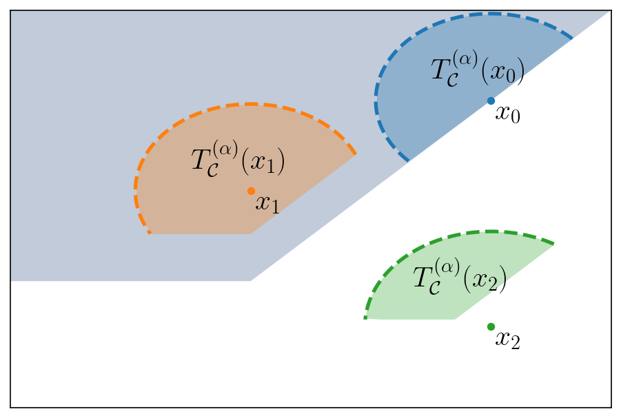
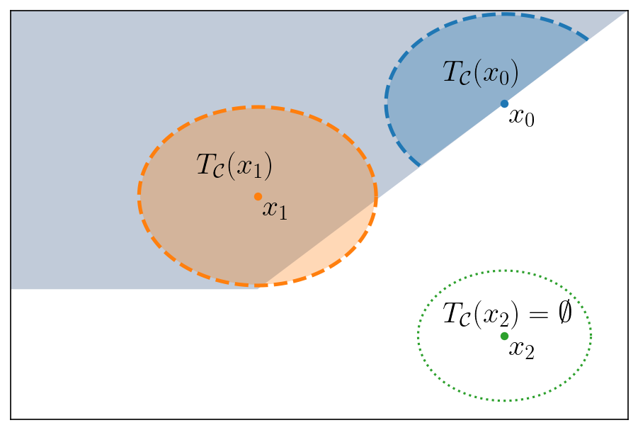
Figure 1: Illustration of the notion of tangent cone, and $\alpha$-restricted tangent set. The gray-shaded region represents the set $\mathcal{C}$. The colored regions depict either type of set, which consists of vectors centered various points $x_{i}$. The dashed border indicates directions in which the magnitude of vectors in the set are unbounded. (a) The $\alpha$-restricted tangent set. Note that the set is well-defined at $x_{2}\not\in\mathcal{C}$, however because the region does not overlap with the point $x_{2}$, the set $T^{(\alpha)}_{\mathcal{C}}(x_{2})$ does not contain any zero vectors, and all vectors point strictly toward the feasible set. (b) The tangent cone. Note that the tangent cone is not well defined at points outside $\mathcal{C}$.

Proposition 5.2.

(Properties of $\alpha$-Restricted Tangent Set) Assume MFCQ holds for all $x\in\mathcal{C}$. The set-valued map $T_{\mathcal{C}}^{(\alpha)}:^{n}\rightrightarrows^{n}$ satisfies:

1. $T_{\mathcal{C}}^{(\alpha)}(x)$ is convex for all $x\in^{n}$;

2. For any fixed $x\in\mathcal{C}$, the set $T^{(\alpha)}_{\mathcal{C}}(x)$ satisfies MFCQ at all $\xi\in T^{(\alpha)}_{\mathcal{C}}(x)$.

3. There exists an open set $X$ containing $\mathcal{C}$ such that $T^{(\alpha)}_{\mathcal{C}}(x)\neq\emptyset$ for all $x\in X$;

4. If $x\in\mathcal{C}$, then $T_{\mathcal{C}}^{(\alpha)}\subset T_{\mathcal{C}}(x)$.

We first observe that (i) follows from the fact that the constraints characterizing $T_{C}^{(\alpha)}(x)$ are affine in the variable $\xi$. We prove (ii) using the same strategy as [3, Lemma 4.5], which we sketch here. If MFCQ holds at $x\in\mathcal{C}$, then the inequalities defining (15) satisfy Slater’s condition [14, Chapter 5.2.3] at $x$ and therefore MFCQ holds for all $\xi\in T^{(\alpha)}_{\mathcal{C}}(x)$. To show (iii), we note that Slater’s condition implies that the affine constraints parameterizing $T^{(\alpha)}_{\mathcal{C}}(x)$ are regular [38, Theorem 2], meaning that the system remains feasible with respect to perturbations. Since $T^{(\alpha)}_{\mathcal{C}}(x)$ is nonempty for all $x\in\mathcal{C}$, it follows that there exists an open set $X$ containing $\mathcal{C}$ such that $T^{(\alpha)}_{\mathcal{C}}(x)$ is nonempty for all $x\in X$. Finally, (iv) follows from the definition of the tangent cone. ∎

Using the $\alpha$-restricted tangent set, we can define the projected dynamical system

$$\dot{x} =\Pi_{T^{(\alpha)}_{\mathcal{C}}(x)}(-F(x))$$ (16)

$$=\underset{\xi\in^{n}}{\text{argmin}}\quad\frac{1}{2}\left\lVert\xi+F(x)\right\rVert^{2}$$

$$\quad\text{subject to}\quad\frac{\partial g(x)}{\partial x}\xi\leq-\alpha g(x)$$

$$\quad\phantom{subjectto}\quad\frac{\partial h(x)}{\partial x}\xi=-\alpha h(x).$$

Similar to the projected monotone flow, the projection operation ensures that the trajectories of the system remain in the safety set. However, as we show next, the advantages of projecting onto the restricted tangent cone is that the system is well defined for infeasible initial conditions, and trajectories of the system are smooth.

5.3 Properties of Safe Monotone Flow

We now discuss the properties of the safe monotone flow. We begin by establishing the equivalence of the control-based and projection-based implementations. Next, we discuss its stability and safety properties.

5.3.1 Equivalence of Control-Based and Projection-Based Implementations

We establish here that the control-based and projection-based implementations of the safe monotone flow are equivalent. The next result states that the closed-loop dynamics resulting from the implementation of (6) over (7) is equivalent to the projection onto $T^{(\alpha)}_{\mathcal{C}}(x)$. The structure of the proof mirrors that of Proposition 4.2.

Proposition 5.3.

(Equivalence of Control-Based and Projection-Based Implementations) Assume MFCQ holds for everywhere on $\mathcal{C}$ and let $X\subset^{n}$ be an open set containing $\mathcal{C}$ on which $K_{\text{cbf},\alpha}$ takes nonempty values. Let $(u,v)$ be any solution to (14) at $x\in X$ (note that $\mathcal{G}_{\alpha}(x)=\mathcal{F}(x,u,v)$). Then, $\mathcal{G}_{\alpha}(x)=\Pi_{T^{(\alpha)}_{\mathcal{C}}(x)}(-F(x))$.

Let $(u,v)$ be any solution to (14) and $\xi=\Pi_{T^{(\alpha)}_{\mathcal{C}}(x)}(-F(x))$. Then $\mathcal{F}(x,u,v)\in T^{(\alpha)}_{\mathcal{C}}(x)$, so it follows immediately by optimality of $\xi$ that $\left\lVert\xi+F(x)\right\rVert^{2}\leq\left\lVert\mathcal{F}(x,u,v)+F(x)\right\rVert^{2}$. Next, because $\xi$ is given by a projection, there exists $w\in N_{T}(\xi)$, where $T=T^{(\alpha)}_{\mathcal{C}}(x)$ such that $\xi+F(x)+w=0$, see e.g., [17, Corollary 2], and where

$$w=\sum_{i=1}^{m}\bar{u}_{i}\nabla g_{i}(x)+\sum_{j=1}^{k}\bar{v}_{j}\nabla h_{j}(x),\quad\bar{u}\geq 0,$$

$$\bar{u}^{\top}(\nabla g(x)^{\top}+\alpha g(x))=0.$$

Combining this expression with the fact that $\xi=-F(x)-w\in T^{(\alpha)}_{\mathcal{C}}(x)$ and using the definition of the $\alpha$-restricted tangent cone, we deduce that $(\bar{u},\bar{v})\in K_{\text{cbf},\alpha}(x)$. By optimality of $(u,v)$, we have

$$\left\lVert\xi+F(x)\right\rVert^{2} =\big{\|}\sum_{i=1}^{m}\bar{u}_{i}\nabla g_{i}(x)+\sum_{j=1}^{k}\bar{v}_{j}\nabla h_{j}(x)\big{\|}^{2}$$

$$\geq\big{\|}\sum_{i=1}^{m}u_{i}\nabla g_{i}(x)+\sum_{j=1}^{k}v_{j}\nabla h_{j}(x)\big{\|}^{2}$$

$$=\left\lVert\mathcal{F}(x,u,v)+F(x)\right\rVert^{2}.$$

But since the projection onto the $\alpha$-restricted tangent cone must be unique, we conclude $\xi=\mathcal{F}(x,u,v)$. ∎

5.3.2 Existence and Uniqueness of Solutions

We now discuss conditions for the existence and uniqueness of solutions of the safe monotone flow.

Proposition 5.4.

(Existence and Uniqueness of Solutions to Safe Monotone Flow) Assume MFCQ and the constant-rank condition hold on $\mathcal{C}$ for all $x\in\mathcal{C}$ and let $X$ be the open set containing $\mathcal{C}$ in Proposition 5.2(iii). Then

1. For all $x_{0}\in\mathcal{C}$, there exists a unique solution $x:_{\geq 0}\to^{n}$ to the safe monotone flow with $x(0)=x_{0}$.

2. For all $x_{0}\in X$, there exists a unique solution $x:[0,t_{f}]\to^{n}$ such that $x(0)=x_{0}$. Furthermore, the solution can be extended so that either $t_{f}=\infty$ or $x(t)\to\partial X$ as $t\to t_{f}$.

We first note that the program (16) satisfies the General Strong Second-Order Sufficient Condition (cf. [34]) and Slater’s condition at $x\in X$. Because the objective function and constraints of (16) are twice continuously differentiable, we can apply [34, Theorem 3.6] to conclude that $\mathcal{G}_{\alpha}$ is locally Lipschitz at $x$. Therefore, $\mathcal{G}_{\alpha}$ is also lower semicontinuous and by [8, Chapter 2, Theorem 1] there exists for all $x_{0}\in X$ a solution $x:[0,t_{f}]\to^{n}$ for some $t_{f}>0$ with $x(0)=x_{0}$. Furthermore, either $t_{f}=\infty$ or $x(t)\to\partial X$ as $t\to t_{f}$. Uniqueness of solutions holds by local Lipschitznes and (ii) follows.

To show (i), we note that $\mathcal{G}_{\alpha}(x)\in T_{\mathcal{C}}(x)$, and by [12, Theorem 3.1], for any solution with $x(0)\in\mathcal{C}$, we have that $x(t)\in\mathcal{C}$ for all $t\geq 0$ on the interval on which the solution exists. Since $\mathcal{C}\subset\text{int}(X)$, solutions beginning in $\mathcal{C}$ cannot approach $\partial X$, and exist for all time.

5.3.3 Safety of Safe Monotone Flow

Here we establish the safety properties of the safe monotone flow. We begin by characterizing optimality conditions for the closed-loop dynamics.

Lemma 5.5.

(Optimality Conditions for Closed-loop Dynamics) For $x\in^{n}$, consider the equations

$$\xi+F(x)+\frac{\partial g(x)}{\partial x}^{\top}u+\frac{\partial h(x)}{\partial x}^{\top}v =0,$$ (17a)

$$\frac{\partial g(x)}{\partial x}\xi+\alpha g(x) \leq 0,$$ (17b)

$$\frac{\partial h(x)}{\partial x}\xi+\alpha h(x) =0,$$ (17c)

$$u \geq 0,$$ (17d)

$$u^{\top}\Big{(}\frac{\partial g(x)}{\partial x}\xi+\alpha g(x)\Big{)} =0,$$ (17e)

in $(\xi,u,v)$. Let $\Lambda_{\alpha}:^{n}\rightrightarrows^{m}_{\geq 0}\times^{k}$ be

$$\Lambda_{\alpha}(x)=\{(u,v)\mid\exists\xi\text{ such that }(\xi,u,v)\text{ solves~{}\eqref{eq:KKT_proj}}\}.$$

Assume MFCQ holds everywhere on $\mathcal{C}$. Then, there exists an open set $X\supset\mathcal{C}$ such that, if $x\in X$, then $\Lambda_{\alpha}(x)\neq\emptyset$. If $(\xi,u,v)$ solves (17), then $\mathcal{G}_{\alpha}(x)=\xi$ and $(u,v)$ solves (14).

Let $\tilde{F}(x,\xi)=F(x)+\xi$. Then

$$\xi=\Pi_{T^{(\alpha)}_{\mathcal{C}}(x)}(-F(x))$$

is a solution to the monotone variational inequality $\textnormal{VI}(\tilde{F}(x,\cdot),T^{(\alpha)}_{\mathcal{C}}(x))$, parameterized by $x$. Since MFCQ holds at all $\xi\in T^{(\alpha)}_{\mathcal{C}}(x)$ by Proposition 5.2(iii), we can use the KKT conditions to characterize $\mathcal{G}_{\alpha}(x)$, which correspond to (17). Further, by Proposition 5.2(iv), solutions to (17) exist on an open set $X$ containing $\mathcal{C}$. Since $\tilde{F}$ is strongly monotone with respect to $\xi$, the solution to $\textnormal{VI}(\tilde{F}(x,\cdot),T^{(\alpha)}_{\mathcal{C}}(x))$ is unique, proving the result. ∎

We rely on the optimality conditions in Lemma 5.5 to establish the following result characterizing the equilibria and safety properties of the safe monotone flow.

Theorem 5.6.

(Equilibria and Safety of Safe Monotone Flow) Let $\alpha>0$, $\mathcal{C}$ be convex, and suppose MFCQ and the constant rank condition holds everywhere on $\mathcal{C}$. The following hold for the safe monotone flow:

1. $\mathcal{C}$ is forward invariant and asymptotically stable on $X$;

2. $x^{*}$ is an equilibrium if and only if $x^{*}\in\textnormal{SOL}(F,\mathcal{C})$;

To show (i), note that by Proposition 5.3, for all $x\in X$ there exists $(u(x),v(x))\in K_{\text{cbf},\alpha}(x)$ such that $\mathcal{G}_{\alpha}(x)=\mathcal{F}(x,u(x),v(x))$. Given the existence and uniqueness of solutions of the closed-loop system, cf. Propositions 5.4, the result follows from Lemma 2.2 since $\phi(x)=(g(x),h(x))$ is a VCBF. Statement (ii) follows from the observation that, if $\mathcal{G}_{\alpha}(x^{*})=0$, by Lemma 5.5, there exists $(u^{*},v^{*})$ such that $(0,u^{*},v^{*})$ solves (17), which holds if and only if $(x^{*},u^{*},v^{*})$ solves (3). ∎

5.3.4 Stability of Safe Monotone Flow

Here we characterize the stability properties of the safe monotone flow. We begin by establishing conditions for stability relative to $\mathcal{C}$.

Theorem 5.7.

(Stability of Safe Monotone Flow Relative to $\mathcal{C}$) Assume MFCQ holds everywhere on $\mathcal{C}$. Then

1. If $x^{*}\in\textnormal{SOL}(F,\mathcal{C})$ and $F$ is monotone, then $x^{*}$ is globally Lyapunov stable relative to $\mathcal{C}$;

2. If $x^{*}\in\textnormal{SOL}(F,\mathcal{C})$ and $F$ is $\mu$-strongly monotone, then $x^{*}$ is globally asymptotically stable relative to $\mathcal{C}$.

Before proving Theorem 5.7, we provide several intermediate results. Our strategy relies on fixing $x^{*}\in\textnormal{SOL}(F,\mathcal{C})$ and considering the candidate Lyapunov function

$$V(x)\!=\!\underbrace{\frac{1}{2}\left\lVert x-x^{*}\right\rVert^{2}}_{\tilde{V}(x)}\!-\frac{1}{\alpha^{2}}\!\underbrace{\inf_{\xi\in T^{(\alpha)}_{\mathcal{C}}(x)}\!\!\!\big{\{}\xi^{\top}F(x)\!+\!\frac{1}{2}\left\lVert\xi\right\rVert^{2}\!\big{\}}}_{W(x)}\!.$$ (18)

We first compute bounds on the Dini derivative of $\tilde{V}$ along $\mathcal{G}_{\alpha}$.

Lemma 5.8.

(Dini Derivative of $\tilde{V}$) Assume MFCQ holds everywhere on $\mathcal{C}$. For $x^{*}\in\textnormal{SOL}(F,\mathcal{C})$, let $(u^{*},v^{*})$ be Lagrange multipliers corresponding to $x^{*}$. For $x\in X$ and $(u,v)\in\Lambda_{\alpha}(x)$, then

$$D^{+}_{\mathcal{G}_{\alpha}} \tilde{V}(x)\leq-\mu\left\lVert x-x^{*}\right\rVert^{2}$$

$$-(u-u^{*})^{\top}(g(x)-g(x^{*}))-(v-v^{*})^{\top}h(x),$$

if $F$ is $\mu$-strongly monotone (inequality holds with $\mu=0$ if F is monotone instead).

Note that

$$D^{+}_{\mathcal{G}_{\alpha}}\tilde{V}(x)=-(x-x^{*})^{\top}F(x)$$

$$\quad-\sum_{i=1}^{m}u_{i}(x-x^{*})^{\top}\nabla g_{i}(x)-\sum_{j=1}^{k}v_{j}(x-x^{*})^{\top}\nabla h_{j}(x).$$

By $\mu$-strong monotonicity of $F$, $-(x-x^{*})^{\top}F(x)\leq-\mu\left\lVert x-x^{*}\right\rVert^{2}-(x-x^{*})^{\top}F(x^{*})$ (the inequality holds with $\mu=0$ if $F$ is monotone). Next, we rearrange (3a) and use that $g_{i}$ is convex for all $i=1,\dots,m$ and $h_{j}$ is affine for all $j=1,\dots,m$ to obtain

$$- (x-x^{*})^{\top}F(x^{*})$$

$$=\sum_{i=1}^{m}u_{i}^{*}(x-x^{*})^{\top}\nabla g_{i}(x^{*})+\sum_{j=1}^{k}v_{j}^{*}(x-x^{*})^{\top}\nabla h_{j}(x^{*})$$

$$\leq\sum_{i=1}^{m}u_{i}^{*}(g_{i}(x)-g_{i}(x^{*}))+\sum_{j=1}^{k}v_{j}^{*}(h_{j}(x)-h_{j}(x^{*}))$$

$$=(u^{*})^{\top}(g(x)-g(x^{*}))+(v^{*})^{\top}h(x).$$

where the last equality follows from the fact that $h(x^{*})=0$. By a similar line of reasoning, we have

$$-\sum_{i=1}^{m}u_{i}(x-x^{*})^{\top}\nabla g_{i}(x)-\sum_{j=1}^{k}v_{j}(x-x^{*})^{\top}\nabla h_{j}(x)$$

$$\leq-\sum_{i=1}^{m}u_{i}(g_{i}(x)-g_{i}(x^{*}))-\sum_{j=1}^{k}v_{j}(h_{j}(x)-h_{j}(x^{*}))$$

$$=-u^{\top}(g(x)-g(x^{*}))-v^{\top}h(x).$$

The result follows by summing the two expressions. ∎

We now move on to characterizing properties of $W$.

Lemma 5.9.

(Properties of $W$) Assume MFCQ holds everywhere on $\mathcal{C}$. Define the matrix-valued function $Q:X\times^{m}_{\geq 0}\to^{n\times n}$ by

$$Q(x,u)=\frac{1}{2}\Big{(}\frac{\partial F(x)}{\partial x}+\frac{\partial F(x)}{\partial x}^{\top}\Big{)}+\sum_{i=1}^{m}u_{i}\nabla^{2}g_{i}(x).$$

Then, for all $x\in X$ and $(u,v)\in\Lambda_{\alpha}(x)$,

$$W(x)=-\frac{1}{2}\left\lVert\mathcal{G}_{\alpha}(x)\right\rVert^{2}+\alpha u^{\top}g(x)+\alpha v^{\top}h(x)$$ (19)

and

$$D^{+}_{\mathcal{G}_{\alpha}}W(x) \geq\mathcal{G}_{\alpha}(x)^{\top}Q(x,u)\mathcal{G}_{\alpha}(x)$$ (20)

$$\quad-\alpha^{2}u^{\top}g(x)-\alpha^{2}v^{\top}h(x).$$

We first show that the solution to the optimization problem in the definition of $W$ is $\xi=\mathcal{G}_{\alpha}(x)$. Note that the constraints in the definition of $W$ in (18) and (16) are identical. Let $J(x,\xi)$ denote the objective function in the definition of $W$. Then $J(x,\xi)-\frac{1}{2}\left\lVert\xi+F(x)\right\rVert^{2}=-\frac{1}{2}\left\lVert F(x)\right\rVert^{2}$. Because the difference between the objective functions of (16) and the definition of $W$ is independent of $\xi$, the two optimization problems have the same solution. The claim now follows because the solution to (16) is $\mathcal{G}_{\alpha}(x)$.

Next we show that $W$ can be expressed in closed form as (19). Because the optimizer is $\xi=\mathcal{G}_{\alpha}(x)$, we have

$$W(x)=\mathcal{G}_{\alpha}(x)^{\top}F(x)+\frac{1}{2}\left\lVert\mathcal{G}_{\alpha}(x)\right\rVert^{2}.$$ (21)

Note that $(\mathcal{G}_{\alpha}(x),u,v)$ satisfies the optimality conditions (17) for all $(u,v)\in\Lambda_{\alpha}(x)$. Therefore we can rearrange (17a) to obtain $F(x)=-\mathcal{G}_{\alpha}(x)-\frac{\partial g(x)}{\partial x}^{\top}u-\frac{\partial h(x)}{\partial x}^{\top}v$. Next

$$\mathcal{G}_{\alpha}(x) {}^{\top}F(x)$$

$$=-\left\lVert\mathcal{G}_{\alpha}(x)\right\rVert^{2}-u^{\top}\frac{\partial g(x)}{\partial x}\mathcal{G}_{\alpha}(x)-v^{\top}\frac{\partial h(x)}{\partial x}\mathcal{G}_{\alpha}(x)$$

$$=-\left\lVert\mathcal{G}_{\alpha}(x)\right\rVert^{2}+\alpha u^{\top}g(x)+\alpha v^{\top}h(x),$$

where the second equality follows by rearranging (17c) and (17e). Then, (19) follows by substituting the previous expression into (21).

Finally we show (20). Let $L(x;\xi,u,v)$ be the Lagrangian of the parametric optimization problem in the definition of $W$ in (18). Then

$$L( x;\xi,u,v)=\xi^{\top}F(x)+\frac{1}{2}\left\lVert\xi\right\rVert^{2}+$$ (22)

$$\sum_{i=1}^{m}u_{i}(\nabla g_{i}(x)^{\top}\xi+\alpha g_{i}(x))+\sum_{i=1}^{k}v_{i}(\nabla h_{i}(x)^{\top}\xi+\alpha h_{i}(x)).$$

Next by [13, Theorem 4.2], it follows that

$$D^{+}_{\mathcal{G}_{\alpha}}W(x)=\sup_{(u,v)\in\Lambda_{\alpha}(x)}\left\{\nabla_{x}L(x;\mathcal{G}_{\alpha}(x),u,v)^{\top}\mathcal{G}_{\alpha}(x)\right\}$$

$$\geq\nabla_{x}L(x;\mathcal{G}_{\alpha}(x),u,v)^{\top}\mathcal{G}_{\alpha}(x).$$

By direct computation, we can verify that

$$\nabla_{x}L(x;\xi,u,v) =Q(x,u)\xi+\alpha\frac{\partial g(x)}{\partial x}^{\top}u+\alpha\frac{\partial h(x)}{\partial x}^{\top}v$$

Therefore

$$\nabla_{x}L(x;\mathcal{G}_{\alpha}(x),u,v)^{\top}\mathcal{G}_{\alpha}(x)=\mathcal{G}_{\alpha}(x)^{\top}Q(x,u)\mathcal{G}_{\alpha}(x)$$

$$\qquad+\alpha u^{\top}\frac{\partial g(x)}{\partial x}\mathcal{G}_{\alpha}(x)+\alpha v^{\top}\frac{\partial h(x)}{\partial x}\mathcal{G}_{\alpha}(x)$$

$$=\mathcal{G}_{\alpha}(x)^{\top}Q(x,u)\mathcal{G}_{\alpha}(x)-\alpha^{2}u^{\top}g(x)-\alpha^{2}v^{\top}h(x),$$

where once again, the last equality above follows by rearranging (17c) and (17e). ∎

We are now ready to prove Theorem 5.7.

[Proof of Theorem 5.7] Let $x^{*}\in\textnormal{SOL}(F,\mathcal{C})$ and suppose the hypotheses of (i) hold. Consider the function $V:X\to$ defined by (18). We show that $V$ is a (strict) Lyapunov function when $F$ is ($\mu$-strongly) monotone. Let $x\in\mathcal{C}$ and $(u,v)\in\Lambda_{\alpha}(x)$. Then, using (17d), $\alpha u^{\top}g(x)+v^{\top}h(x)\leq 0$, so by examining the expression in (19) we see that $W(x)\leq 0$ for all $x\in\mathcal{C}$ with equality if and only if $x\in\textnormal{SOL}(F,\mathcal{C})$. Thus $V$ is positive definite with respect to $x^{*}$. Next, $D^{+}_{\mathcal{G}_{\alpha}}V(x)=D^{+}_{\mathcal{G}_{\alpha}}\tilde{V}(x)-\frac{1}{\alpha^{2}}D^{+}_{\mathcal{G}_{\alpha}}W(x)$, and by Lemmas 5.8 and 5.9,

$$D^{+}_{\mathcal{G}_{\alpha}}V(x)\leq-\frac{1}{\alpha^{2}}\mathcal{G}_{\alpha}(x)Q(x,u)\mathcal{G}_{\alpha}(x)+u^{\top}g(x)+v^{\top}h(x)$$

$$\qquad-(u-u^{*})^{\top}(g(x)-g(x^{*}))(v-v^{*})^{\top}(h(x)-h(x^{*}))$$

$$=-\frac{1}{\alpha^{2}}\mathcal{G}_{\alpha}(x)Q(x,u)\mathcal{G}_{\alpha}(x)$$

$$\qquad+(u^{*})^{\top}g(x)+(v^{*})^{\top}h(x)+u^{\top}g(x^{*})+v^{\top}h(x^{*}).$$

Since $u\geq 0$ and $x^{*}\in\mathcal{C}$, we have $g(x^{*})\leq 0$ and $h(x^{*})=0$, and therefore $u^{\top}g(x^{*})+v^{\top}h(x^{*})\leq 0$. Similarly, since $u^{*}\geq 0$, and $x\in\mathcal{C}$, we have $g(x)\leq 0$ and $h(x)=0$, and therefore $(u^{*})^{\top}g(x)+(v^{*})^{\top}h(x)\leq 0$. Finally, since $F$ is monotone and $g$ is convex, it follows that $Q(x,u)$ is positive semi-definite, and therefore $D^{+}_{\mathcal{G}_{\alpha}}V(x)\leq 0$. To show (ii), we can use the same reasoning above to show that $D^{+}_{\mathcal{G}_{\alpha}}V(x)\leq-\mu\left\lVert x-x^{*}\right\rVert^{2}$. ∎

Next, we discuss stability with respect to the entire state space, which ensures the safe monotone flow can be used to solve $\textnormal{VI}(F,\mathcal{C})$ even for infeasible initial conditions.

Theorem 5.10.

(Stability of Safe Monotone Flow with Respect to ⁿ) Assume MFCQ and the constant-rank condition holds on $\mathcal{C}$. Then

1. If $x^{*}\in\textnormal{SOL}(F,\mathcal{C})$ and $F$ is monotone, then $x^{*}$ is globally Lyapunov stable;

2. If $x^{*}\in\textnormal{SOL}(F,\mathcal{C})$ and $F$ is $\mu$-strongly monotone, then $x^{*}$ is globally asymptotically stable.

To prove Theorem 5.10, we can no longer rely on the Lyapunov function $V$ defined in (18) because it is no longer positive definite and may take negative values for $x\not\in\mathcal{C}$. Instead, we consider the new candidate Lyapunov function

$$V_{\epsilon}(x)=\tilde{V}(x)+\Big{[}-\frac{1}{\alpha^{2}}W(x)\Big{]}_{+}+\delta_{\epsilon}(x)$$ (23)

where $\epsilon>0$ and $\delta_{\epsilon}$ is the penalty function given by

$$\delta_{\epsilon}(x)=\frac{1}{\epsilon}\sum_{i=1}^{m}[g_{i}(x)]_{+}+\frac{1}{\epsilon}\sum_{j=1}^{k}|h_{j}(x)|.$$

Before proceeding to the proof of Theorem 5.10, we provide a bound for the Dini derivative of $\delta_{\epsilon}$ along $\mathcal{G}_{\alpha}$.

Lemma 5.11.

(Dini Derivative of $\delta_{\epsilon}$) For all $x\in X$ and $\xi\in^{n}$, $\delta_{\epsilon}$ is directionally differentiable along $\xi$ at $x$. In particular,

$$D^{+}_{\mathcal{G}_{\alpha}}\delta_{\epsilon}(x)\leq-\frac{\alpha}{\epsilon}\sum_{i\in I_{+}(x)}g_{i}(x)-\frac{\alpha}{\epsilon}\sum_{j\in I_{h}(x)}\left|h_{j}(x)\right|,$$ (24)

where $I_{h}(x)=\{j\in[1,k]\mid h_{j}(x)\neq 0\}$.

Note that $\delta_{\epsilon}$ corresponds to the $\ell^{1}$ penalty function for the set $\mathcal{C}$. By [26, Proposition 3], the directional derivative of $\delta_{\epsilon}$ is

$$\delta^{\prime}_{\epsilon} (x;\xi)=$$

$$\frac{1}{\epsilon}\sum_{i\in I_{+}(x)}\nabla g_{i}(x)^{\top}\xi+\frac{1}{\epsilon}\sum_{i\in I_{0}(x)}[\nabla g_{i}(x)^{\top}\xi]_{+}+$$

$$\frac{1}{\epsilon}\sum_{j\in I_{h}(x)}\textnormal{sgn}(h_{j}(x))\nabla h_{j}(x)^{\top}\xi+\frac{1}{\epsilon}\sum_{j\not\in I_{h}(x)}\left|\nabla h_{j}(x)^{\top}\xi\right|.$$

Note $D^{+}_{\mathcal{G}_{\alpha}}\delta_{\epsilon}(x)=\delta^{\prime}_{\epsilon}(x;\mathcal{G}_{\alpha}(x))$. Expression (24) follows by noting that $\nabla g_{i}(x)^{\top}\mathcal{G}_{\alpha}(x)\leq-\alpha g_{i}(x)$ and $\nabla h_{j}(x)^{\top}\mathcal{G}_{\alpha}(x)=-\alpha h_{j}(x)$. ∎

We are now ready to prove Theorem 5.10.

[Proof of Theorem 5.10] We begin by showing (i). Let $x^{*}\in\textnormal{SOL}(F,\mathcal{C})$. Note that, from the optimality conditions (17), $\Lambda_{\alpha}(x^{*})$ corresponds to the set of Lagrange multipliers of the solution $x^{*}$ to $\textnormal{VI}(F,\mathcal{C})$. Because MFCQ holds at $x^{*}$, it follows that $\Lambda_{\alpha}(x^{*})$ is bounded. Thus, it is possible to choose $\epsilon>0$ small enough so that

$$\frac{\alpha}{\epsilon}>\sup_{(u^{*},v^{*})\in\Lambda_{\alpha}(x^{*})}\big{\{}\left\lVert(u^{*},v^{*})\right\rVert_{\infty}\big{\}}.$$ (25)

Next, it follows immediately from the definition (23) that $V_{\epsilon}$ is positive definite with respect to $x^{*}$. We now compute $D^{+}_{\mathcal{G}_{\alpha}}V_{\epsilon}(x)$ and show that it is negative semidefinite. Let $x\in X$. We consider three cases: $W(x)<0$, $W(x)>0$, and $W(x)=0$. In the case where $W(x)<0$,

$$D^{+}_{\mathcal{G}_{\alpha}}V_{\epsilon}=D^{+}_{\mathcal{G}_{\alpha}}\tilde{V}(x)-\frac{1}{\alpha^{2}}D^{+}_{\mathcal{G}_{\alpha}}W(x)+D^{+}_{\mathcal{G}_{\alpha}}\delta_{\epsilon}(x).$$

Combining the bounds in Lemmas 5.8, 5.9, and 5.11,

$$D^{+}_{\mathcal{G}_{\alpha}}V_{\epsilon}(x)\leq-\frac{1}{\alpha^{2}}\mathcal{G}_{\alpha}(x)Q(x,u)\mathcal{G}_{\alpha}(x)$$ (26)

$$+\sum_{i\in I_{+}(x)}\left(u^{*}-\frac{\alpha}{\epsilon}\right)g_{i}(x)+\sum_{j\in I_{h}(x)}\left(v^{*}-\frac{\alpha}{\epsilon}\right)\left|h_{j}(x)\right|.$$

Since $\epsilon$ satisfies (25), it follows that $D^{+}_{\mathcal{G}_{\alpha}}V_{\epsilon}(x)\leq 0$.

For the case where $W(x)>0$, we rearrange (19) to write

$$u^{\top}g(x)+v^{\top}h(x)=\frac{1}{\alpha}W(x)+\frac{1}{2\alpha}\left\lVert\mathcal{G}(x)\right\rVert^{2}>\frac{1}{2\alpha}\left\lVert\mathcal{G}(x)\right\rVert^{2}.$$

Then, we have

$$D^{+}_{\mathcal{G}_{\alpha}} V_{\epsilon}(x)=D^{+}_{\mathcal{G}_{\alpha}}\tilde{V}(x)+D^{+}_{\mathcal{G}_{\alpha}}\delta_{\epsilon}(x)$$

$$\leq-(u-u^{*})^{\top}g(x)-(v-v^{*})^{\top}h(x)$$

$$\qquad-\frac{\alpha}{\epsilon}\sum_{i\in I_{+}(x)}g_{i}(x)-\frac{\alpha}{\epsilon}\sum_{j\in I_{h}(x)}\left|h_{j}(x)\right|$$

$$\leq-\frac{1}{2\alpha}\left\lVert\mathcal{G}_{\alpha}(x)\right\rVert^{2}+$$ (27)

$$\sum_{i\in I_{+}(x)}\left(u^{*}-\frac{\alpha}{\epsilon}\right)g_{i}(x)+\sum_{j\in I_{h}(x)}\left(v^{*}-\frac{\alpha}{\epsilon}\right)\left|h_{j}(x)\right|,$$

and $D^{+}_{\mathcal{G}_{\alpha}}V_{\epsilon}(x)\leq 0$. In the case where $W(x)=0$,

$$D^{+}_{\mathcal{G}_{\alpha}}V_{\epsilon}(x)=D^{+}_{\mathcal{G}_{\alpha}}\tilde{V}(x)+\frac{1}{\alpha^{2}}[-D^{+}_{\mathcal{G}_{\alpha}}W(x)]_{+}+D^{+}_{\mathcal{G}_{\alpha}}\delta_{\epsilon}(x),$$

which leads us to two subcases: (a) $D^{+}_{\mathcal{G}_{\alpha}}W(x)<0$ and (b) $D^{+}_{\mathcal{G}_{\alpha}}W(x)\geq 0$. In subcase (a), $D^{+}_{\mathcal{G}_{\alpha}}V_{\epsilon}(x)$ satisfies the bound in (26) and, therefore, $D^{+}_{\mathcal{G}_{\alpha}}V_{\epsilon}(x)\leq 0$. In subcase (b), $u^{\top}g(x)+v^{\top}h(x)=\frac{1}{2\alpha}\left\lVert\mathcal{G}_{\alpha}(x)\right\rVert^{2}$ and, therefore, $D^{+}_{\mathcal{G}_{\alpha}}V_{\epsilon}(x)$ satisfies the bound in (5.3.4), so $D^{+}_{\mathcal{G}_{\alpha}}V_{\epsilon}(x)\leq 0$.

Finally, for (ii), we can use the same arguments above to show in each case $D^{+}_{\mathcal{G}_{\alpha}}V_{\epsilon}(x)\leq-\mu\left\lVert x-x^{*}\right\rVert^{2}$. ∎

We conclude this section by discussing the contraction properties of the safe monotone flow. Contraction refers to the property that any two trajectories of the system approach each other exponentially (cf. [24, 18] for a precise definition), and implies exponential stability of an equilibrium. We show that, for sufficiently large $\alpha$, the safe monotone flow system is contracting provided $F$ is globally Lipschitz and the constraint set $\mathcal{C}$ is polyhedral.

Our analysis relies relies on the following result.

Lemma 5.12.

([45, Lemma 2.1]) Consider the following quadratic program

$$\underset{(u,v)\in^{m}_{\geq 0}\times^{k}}{\textnormal{min}}\;\frac{1}{2}\left\lVert\begin{bmatrix}u\\ v\end{bmatrix}\right\rVert_{\tilde{Q}}^{2}+c^{\top}\begin{bmatrix}u\\ v\end{bmatrix}+p,$$ (28)

where $\tilde{Q}\succeq 0$. Then $(u^{*},v^{*})$ solves (28) if and only if it is a solution to the linear program

$$\underset{(u,v)\in^{m}_{\geq 0}\times^{k}}{\textnormal{min}}\left(\tilde{Q}\begin{bmatrix}u^{*}\\ v^{*}\end{bmatrix}+c\right)^{\top}\begin{bmatrix}u\\ v\end{bmatrix}.$$ (29)

We now show that the safe monotone flow is contracting.

Theorem 5.13.

(Contraction and Exponential Stability of Safe Monotone Flow) Let $F$ be $\mu$-strongly monotone and globally Lipschitz with constant $\ell_{F}$ and $\mathcal{C}$ a polyhedral set defined by (2) with $g(x)=Gx-c_{g}$ and $h(x)=Hx-c_{h}$. If

$$\alpha>\frac{\ell_{F}^{2}}{4\mu},$$ (30)

then the safe monotone flow is contracting with rate $c=\mu-\frac{\ell_{F}^{2}}{4\alpha}$. In particular, the unique solution $x^{*}\in\textnormal{SOL}(F,\mathcal{C})$ is globally exponentially stable.

We claim that if the assumptions hold, then

$$(x-y)^{\top}(\mathcal{G}_{\alpha}(x)-\mathcal{G}_{\alpha}(y))\leq-c\left\lVert x-y\right\rVert^{2},$$ (31)

in which case the system is contracting by [24, Theorem 31], and exponential stability of $x^{*}\in\textnormal{SOL}(F,\mathcal{C})$ follows as a consequence. To show the claim, from (17a), note that

$$\mathcal{G}_{\alpha}(x)=-F(x)-G^{\top}u_{x}-H^{\top}v_{x}.$$

for any $(u_{x},v_{x})\in\Lambda_{\alpha}(x)$. Let then $x,y\in X$ and $(u_{x},v_{x})\in\Lambda_{\alpha}(x)$ and $(u_{y},v_{y})\in\Lambda_{\alpha}(y)$. Then, using the strong monotonicity of $F$,

$$(x- y)^{\top}(\mathcal{G}_{\alpha}(x)-\mathcal{G}_{\alpha}(y))=-(x-y)^{\top}(F(x)-F(y))$$

$$+(x-y)^{\top}(\mathcal{G}_{\alpha}(x)+F(x)-\mathcal{G}_{\alpha}(y)-F(y))$$

$$\leq-\mu\left\lVert x-y\right\rVert^{2}-(x-y)^{\top}\begin{bmatrix}G^{\top}&H^{\top}\end{bmatrix}\begin{bmatrix}u_{x}-u_{y}\\ v_{x}-v_{y}\end{bmatrix}$$

$$=-\mu\left\lVert x-y\right\rVert^{2}-\begin{bmatrix}u_{x}-u_{y}\\ v_{x}-v_{y}\end{bmatrix}^{\top}\begin{bmatrix}G(x-y)\\ H(x-y)\end{bmatrix}.$$ (32)

Next, let $\tilde{J}(x;u,v)=-\inf_{\xi\in^{n}}L(x;\xi,u,v)$, where $L$ is the Lagrangian of (16), defined in (22), and let

$$\tilde{Q}=\begin{bmatrix}GG^{\top}&GH^{\top}\\ HG^{\top}&HH^{\top}\end{bmatrix}.$$

For $x\in^{n}$, $L$ is minimized when $\xi=-F(x)-G^{\top}u-H^{\top}v$, and therefore

$$\tilde{J}(x;u,v)= \frac{1}{2}\left\lVert\begin{bmatrix}u\\ v\end{bmatrix}\right\rVert^{2}_{\tilde{Q}}\!\!+\!\begin{bmatrix}GF(x)\!-\!\alpha(Gx-c_{g})\\ HF(x)\!-\!\alpha(Hx-c_{h})\end{bmatrix}^{\top}\!\!\begin{bmatrix}u\\ v\end{bmatrix}$$ (33)

$$+\frac{1}{2}\left\lVert F(x)\right\rVert^{2}.$$

If $(u_{x},v_{x})\in\Lambda_{\alpha}(x)$, then $(u_{x},v_{x})$ is a solution to the program $\min_{(u,v)\in^{m}_{\geq 0}\times^{k}}\tilde{J}(x,u,v)$, which is the Lagrangian dual of (16). By Lemma 5.12, $(u_{x},v_{x})$ is also a solution to the linear program,

$$\underset{(u,v)\in^{m}_{\geq 0}\times^{k}}{\textnormal{min}}\left(\tilde{Q}\begin{bmatrix}u_{x}\\ v_{x}\end{bmatrix}+\begin{bmatrix}GF(x)-\alpha(Gx-c_{g})\\ HF(x)-\alpha(Hx-c_{h})\end{bmatrix}\right)^{\top}\begin{bmatrix}u\\ v\end{bmatrix}.$$

Since $(u_{y},v_{y})$ is also feasible for the previous linear program, by optimality of $(u_{x},v_{x})$,

$$- \begin{bmatrix}u_{x}-u_{y}\\ v_{x}-v_{y}\end{bmatrix}^{\top}\begin{bmatrix}Gx-c_{g}\\ Hx-c_{h}\end{bmatrix}\leq-\frac{1}{\alpha}\left\lVert\begin{bmatrix}u_{x}\\ v_{x}\end{bmatrix}\right\rVert^{2}_{\tilde{Q}}$$

$$+\frac{1}{\alpha}\begin{bmatrix}u_{y}\\ v_{y}\end{bmatrix}^{\top}\tilde{Q}\begin{bmatrix}u_{x}\\ v_{x}\end{bmatrix}-\frac{1}{\alpha}\begin{bmatrix}u_{x}-u_{y}\\ v_{x}-v_{y}\end{bmatrix}^{\top}\begin{bmatrix}GF(x)\\ HF(x)\end{bmatrix}.$$

By a similar line of reasoning,

$$- \begin{bmatrix}u_{y}-u_{x}\\ v_{y}-v_{x}\end{bmatrix}^{\top}\begin{bmatrix}Gy-c_{g}\\ Hy-c_{h}\end{bmatrix}\leq-\frac{1}{\alpha}\left\lVert\begin{bmatrix}u_{y}\\ v_{y}\end{bmatrix}\right\rVert^{2}_{\tilde{Q}}$$

$$+\frac{1}{\alpha}\begin{bmatrix}u_{x}\\ v_{x}\end{bmatrix}^{\top}\tilde{Q}\begin{bmatrix}u_{y}\\ v_{y}\end{bmatrix}-\frac{1}{\alpha}\begin{bmatrix}u_{y}-u_{x}\\ v_{y}-v_{x}\end{bmatrix}^{\top}\begin{bmatrix}GF(y)\\ HF(y)\end{bmatrix}.$$

Combining the previous two expressions, we obtain

$$-\begin{bmatrix}u_{x}-u_{y}\\ v_{x}-v_{y}\end{bmatrix}^{\top}\begin{bmatrix}G(x-y)\\ H(x-y)\end{bmatrix}$$

$$\leq-\frac{1}{\alpha}\begin{bmatrix}u_{x}-u_{y}\\ v_{x}-v_{y}\end{bmatrix}^{\top}\begin{bmatrix}G(F(x)-F(y))\\ H(F(x)-F(y))\end{bmatrix}-\frac{1}{\alpha}\left\lVert\begin{bmatrix}u_{x}-u_{y}\\ v_{x}-v_{y}\end{bmatrix}\right\rVert^{2}_{\tilde{Q}}$$

$$\leq\frac{\ell_{F}}{\alpha}\left\lVert\begin{bmatrix}G\\ H\end{bmatrix}^{\top}\begin{bmatrix}u_{x}-u_{y}\\ v_{x}-v_{y}\end{bmatrix}\right\rVert\left\lVert x-y\right\rVert-\frac{1}{\alpha}\left\lVert\begin{bmatrix}G\\ H\end{bmatrix}^{\top}\begin{bmatrix}u_{x}-u_{y}\\ v_{x}-v_{y}\end{bmatrix}\right\rVert^{2}\!\!,$$

where we used $\|(u,v)\|_{\tilde{Q}}=\left\lVert M^{\top}(u,v)\right\rVert$, with $M=[G;H]$. For any $\epsilon>0$, by Young’s Inequality [41, pp. 140],

$$-\begin{bmatrix}u_{x}-u_{y}\\ v_{x}-v_{y}\end{bmatrix}^{\top} \begin{bmatrix}G(x-y)\\ H(x-y)\end{bmatrix}\leq\frac{\ell_{F}}{2\epsilon\alpha}\left\lVert x-y\right\rVert^{2}$$

$$-\Big{(}\frac{1}{\alpha}-\frac{\epsilon\ell_{F}}{2\alpha}\Big{)}\left\lVert\begin{bmatrix}G\\ H\end{bmatrix}^{\top}\begin{bmatrix}u_{x}-u_{y}\\ v_{x}-v_{y}\end{bmatrix}\right\rVert^{2}\!\!.$$

Substituting into (5.3.4), we obtain

$$(x-y)^{\top} (\mathcal{G}_{\alpha}(x)-\mathcal{G}_{\alpha}(y))\leq-\Big{(}\mu-\frac{\ell_{F}}{2\epsilon\alpha}\Big{)}\left\lVert x-y\right\rVert^{2}$$

$$-\Big{(}\frac{1}{\alpha}-\frac{\epsilon\ell_{F}}{2\alpha}\Big{)}\left\lVert\begin{bmatrix}G\\ H\end{bmatrix}^{\top}\begin{bmatrix}u_{x}-u_{y}\\ v_{x}-v_{y}\end{bmatrix}\right\rVert^{2}.$$

Therefore, (31) holds with $c=\mu-\frac{\ell_{F}}{2\epsilon\alpha}$ if $\epsilon$ satisfies $\frac{\ell_{F}}{2\alpha\mu}\leq\epsilon\leq\frac{2}{\ell_{F}}$. Such $\epsilon$ can be chosen if $\alpha>\frac{\ell_{F}^{2}}{4\mu}$, which corresponds to the condition (30). The optimal estimate of the contraction rate is $c=\mu-\frac{\ell_{F}^{2}}{4\alpha}$. ∎

Remark 5.14.

(Connection with Safe Gradient Flow) The safe monotone flow is a generalization of the safe gradient flow introduced in [3]. The latter was originally studied in the context of nonconvex optimization and, similar to the case of the safe monotone flow, enjoys safety of the feasible set and correspondence between equilibria and critical points. Further, under certain constraint qualifications, the local stability of equilibria relative to the constraint set under the safe gradient flow can be established using the objective function as a Lyapunov function. Because we are working with variational inequalities, $F$ may not correspond to the gradient of a scalar objective function, so the Lyapunov functions used in [3] are not directly applicable. The assumption of convexity and monotonicity here allows us to construct novel Lyapunov functions to obtain global stability results. $\bullet$

6 Recursive Safe Monotone Flow

A drawback of the projected and safe monotone flows is that, in order to implement them, one needs to solve either the quadratic programs (9) or (14) at each time along the trajectory of the system. As a third algorithmic solution to Problem 1, in this section we introduce the recursive safe monotone flow which gets around this limitation by incorporating a dynamics whose equilibria correspond to the solutions of the quadratic program. We begin by showing how to derive the dynamics for general constraint sets $\mathcal{C}$ by interconnecting two systems on multiple time scales. Next, we use the theory of singular perturbations of contracting flows to obtain stability guarantees in the case where $\mathcal{C}$ is polyhedral, and show that trajectories of the recursive safe monotone flow track those of the safe monotone flow. The latter property enables us to formalize a notion of “practical safety” that the recursive safe monotone flow satisfies.

6.1 Construction of the Dynamics

We discuss here the construction of the recursive safe monotone flow. The starting point for our derivation is the control-affine system (7). The safe monotone flow consists of this system with a feedback controller specified by the quadratic program (14). Rather than solving this program exactly, the approach we take is to replace it with a monotone variational inequality parameterized by the state. For fixed $x\in X$, we can solve solve this inequality, and hence obtain the feedback $k(x)$, using the safe monotone flow corresponding to this problem. Coupling this flow with the control system (7) yields the recursive safe monotone flow.

In this section we carry out this strategy in mathematically precise terms. We rely on the following result, which provides an alternative characterization of the CBF-QP (14).

Lemma 6.1.

(Alternative Characterization of Safe Feedback) For $x\in^{n}$, consider the optimization

$$\underset{(u,v)\in_{\geq 0}^{m}\times^{k}}{\textnormal{minimize}}\;\frac{1}{2}\big{\|}\sum_{i=1}^{m}u_{i}\nabla g_{i}(x)+\sum_{j=1}^{k}v_{j}\nabla h_{j}(x)\big{\|}^{2}$$ (34)

$$+u^{\top}\Big{(}\frac{\partial g}{\partial x}F(x)-\alpha g(x)\Big{)}+v^{\top}\Big{(}\frac{\partial h}{\partial x}F(x)-\alpha h(x)\Big{)}.$$

If $(u,v)$ is a solution to (34), then $(u,v)$ is a solution to (14).

Note that the constraints of (34) satisfy MFCQ for all $(u,v)\in^{m}_{\geq 0}\times^{k}$. Since the objective function in (34) is convex in $(u,v)$, one can see that necessary and sufficient conditions for optimality are given by a KKT system that, after some manipulation, takes the form

$$-\frac{\partial g}{\partial x}\frac{\partial g}{\partial x}^{\top}u-\frac{\partial g}{\partial x}\frac{\partial h}{\partial x}^{\top}v-\frac{\partial g}{\partial x}F(x)-\alpha g(x) \leq 0$$

$$-\frac{\partial h}{\partial x}\frac{\partial g}{\partial x}^{\top}u-\frac{\partial h}{\partial x}\frac{\partial h}{\partial x}^{\top}v-\frac{\partial h}{\partial x}F(x)-\alpha h(x) =0$$

$$u \geq 0$$

$$u^{\top}\Big{(}-\frac{\partial g}{\partial x}\frac{\partial g}{\partial x}^{\top}u-\frac{\partial g}{\partial x}\frac{\partial h}{\partial x}^{\top}v-\frac{\partial g}{\partial x}F(x)-\alpha g(x)\Big{)} =0.$$

It follows immediately that if $(u,v)$ satisfies the above equations, then $(u,v)\in K_{\text{cbf},\alpha}(x)$ given by (13). ∎

The rationale for considering (34), rather than working with (14) directly, is that the constraints of (34) are independent of $x$, which will be important for reasons we show next. Being a constrained optimization problem, (34) can be expressed in terms of a variational inequality (parameterized by $x\in^{n}$). Formally, let $\tilde{F}(x,u,v)$ be given by

$$\tilde{F}(x,u,v)=\begin{bmatrix}-\frac{\partial g}{\partial x}\mathcal{F}(x,u,v)-\alpha g(x)\\ -\frac{\partial h}{\partial x}\mathcal{F}(x,u,v)-\alpha h(x)\end{bmatrix},$$ (35)

where $\mathcal{F}$ is given by (7) and let $\tilde{\mathcal{C}}=^{m}_{\geq 0}\times^{k}$, which we parameterize as

$$\tilde{\mathcal{C}}=\{(u,v)\in^{m}\times^{k}\mid u\geq 0\}.$$ (36)

The optimization problem (34) corresponds to the variational inequality $\textnormal{VI}(\tilde{F}(x,\cdot,\cdot),\tilde{\mathcal{C}})$.

Our next step is to write down the safe monotone flow with safety parameter $\beta>0$ corresponding to the variational inequality $\textnormal{VI}(\tilde{F}(x,\cdot),\tilde{\mathcal{C}})$. Note that the $\beta$-restricted tangent set (15) of $\tilde{\mathcal{C}}$ is

$$T^{(\beta)}_{\tilde{\mathcal{C}}}(u,v)=\Big{\{}(\xi_{u},\xi_{v})\in^{m}\times^{k}\mid\xi_{u}\geq-\beta u\Big{\}}.$$

The projection onto $T^{(\beta)}_{\tilde{\mathcal{C}}}(u,v)$ has the following closed-form solution

$$\Pi_{T^{(\beta)}_{\tilde{\mathcal{C}}}(u,v)}\left(\begin{bmatrix}a\\ b\end{bmatrix}\right)=\begin{bmatrix}\max\{-\beta u,a\}\\ b\end{bmatrix}.$$

Using this expression and applying Proposition 5.3, we write the safe monotone flow corresponding to $\textnormal{VI}(\tilde{F}(x,\cdot),\tilde{\mathcal{C}})$ as

$$\dot{u} =\max\Big{\{}-\beta u,\frac{\partial g(x)}{\partial x}\mathcal{F}(x,u,v)+\alpha g(x)\Big{\}}$$ (37)

$$\dot{v} =\frac{\partial h(x)}{\partial x}\mathcal{F}(x,u,v)+\alpha h(x).$$

Under certain assumptions, which we formalize in the sequel, for a fixed $x$, trajectories of (37) converge to solutions of the QP (14).

This discussion suggests a system solving the original variational inequality $\textnormal{VI}(F,\mathcal{C})$ can be obtained by coupling (37) with the dynamics (7) as follows:

$$\dot{x} =\mathcal{F}(x,u,v)$$ (38a)

$$\tau\dot{u} =\max\Big{\{}-\beta u,\frac{\partial g(x)}{\partial x}\mathcal{F}(x,u,v)+\alpha g(x)\Big{\}}$$ (38b)

$$\tau\dot{v} =\frac{\partial h(x)}{\partial x}\mathcal{F}(x,u,v)+\alpha h(x).$$ (38c)

We refer to the system (38) as the recursive safe monotone flow. The parameter $\tau$ characterizes the separation of timescales between the system (38a) and (38b)-(38c). The interpretation of the dynamics is that, when $\tau>0$ are sufficiently small, (38b)-(38c) evolve on a much faster timescale and rapidly approach the solution set of (14). The system on the slower timescale (38a) then approximates the safe monotone flow. We formalize this analysis next.

6.2 Stability of Recursive Safe Monotone Flow

To prove stability of the system (38), we rely on results from contraction theory [24]. Specifically, we derive conditions on the time-scale separation $\tau$ that ensures that (38) is contracting and, as a consequence, globally attractive and locally exponentially stable. Throughout the section, we assume the following assumption holds.

Assumption 1.

(Strong Monotonicity, Lipschitzness, and Polyhedral Constraints) The following holds:

1. $F$ is $\mu$-strongly monotone and $\ell_{F}$-Lipschitz;

2. $\mathcal{C}$ is a polyhedral set defined by (2) with $g(x)=Gx-c_{g}$ and $h(x)=Hx-c_{h}$, and the matrix

   $$\tilde{Q}=\begin{bmatrix}GG^{\top}&GH^{\top}\\ HG^{\top}&HH^{\top}\end{bmatrix}$$ (39)

   has full rank.

Next, we show that it is possible to tune the parameters $\beta$ so the system (37) is contracting, uniformly in $x$.

Lemma 6.2.

(Contractivity of (37)) Under Assumption 1, if $\beta>\frac{1}{4}\frac{\lambda_{\textnormal{max}}(\tilde{Q})}{\lambda_{\textnormal{min}}(\tilde{Q})},$ then the system (37) is contracting with rate $\bar{c}=\lambda_{\textnormal{min}}(\tilde{Q})-\frac{\lambda_{\textnormal{max}}(\tilde{Q})}{4\beta}$ uniformly in $x$.

We first observe that $\tilde{F}$ is given by

$$\tilde{F}(x,u,v)=\tilde{Q}\begin{bmatrix}u\\ v\end{bmatrix}-\alpha\begin{bmatrix}Gx-c_{g}\\ Hx-c_{h}\end{bmatrix}.$$

By Assumption 1, $\tilde{Q}\succ 0$ and therefore $\tilde{F}$ is (i) $\lambda_{\textnormal{min}}(\tilde{Q})$-strongly monotone in $(u,v)$ uniformly in $x$ and (ii) $\|\tilde{Q}\|$-Lipschitz in $(u,v)$ uniformly in $x$. By Theorem 5.13, if $\beta>\frac{\|\tilde{Q}\|^{2}}{4\lambda_{\textnormal{min}}(\tilde{Q})}$, the system (37) is uniformly contracting. The result follows by observing that $\|\tilde{Q}\|^{2}=\lambda_{\textnormal{max}}(\tilde{Q})$. ∎

We now characterize the contraction and stability properties of the recursive safe monotone flow.

Theorem 6.3.

(Contractivity of Recursive Safe Monotone Flow) Assume $F$ is $\mu$-strongly monotone and $\ell_{F}$ globally Lipschitz, and $\alpha$ satisfies (30). Under Assumption 1 and $\beta$ chosen as in Lemma 6.2, then

1. the unique KKT triple, $(x^{*},u^{*},v^{*})$ corresponding to $\textnormal{VI}(F,\mathcal{C})$ is the only equilibrium of (38).

Moreover, for all $\epsilon>0$, there exists $\tau^{*}>0$, such that for all $0<\tau<\tau^{*}$,

1. the system (38) is contracting on the set

   $$\mathcal{Z}_{\epsilon}=\big{\{}(x,u,v)\in X\times^{m}\times^{k}\mid$$

   $$\left\lVert(u,v)-k(x)\right\rVert\leq\epsilon\big{\}},$$

   and every solution of (38) eventually enters $\mathcal{Z}_{\epsilon}$ in finite time. In particular, there exists a class $\mathcal{K}\mathcal{L}$ function $\beta:_{\geq 0}\times_{\geq 0}\to$ such that for every solution $(x(t),u(t),v(t))$

   $$\left\lVert\big{(}u(x(t)),v(x(t))\big{)}-k(x(t))\right\rVert$$

   $$\leq\beta\big{(}\left\lVert\big{(}u(x(0)),v(x(0))\big{)}-k(x(0))\right\rVert,t\big{)};$$

2. the unique KKT triple $(x^{*},u^{*},v^{*})$ is locally exponentially stable and globally attracting.

We begin with (i). By direct examination of (38), we see that the equilibria correspond exactly with triples satisfying (3). Since the matrix $\tilde{Q}$ has full rank, the gradients of all the constraints are linearly independent, and hence MFCQ holds on $\mathcal{C}$. Since $F$ is $\mu$-strongly monotone, the solution $x^{*}\in\textnormal{SOL}(F,\mathcal{C})$ is unique and there exists a unique Lagrange multiplier $(u^{*},v^{*})$ such that $(x^{*},u^{*},v^{*})$ satisfies (3).

To show (ii), we verify that all hypotheses in [22, Theorem 4] hold. First, note that the map $x\mapsto\mathcal{F}(x,u,v)$ is $\ell_{F}$-Lipschitz in $x$ uniformly in $(u,v)$, and $\left\lVert[G;H]\right\rVert$-Lipschitz in $(u,v)$, uniformly in $x$. Let $\mathcal{H}$ denote the righthand side of (37). Because $\mathcal{H}$ is piecewise affine in $(u,v)$ and $F$ globally Lipschitz, there exists constants $\ell_{\mathcal{H},x}$, $\ell_{\mathcal{H},u,v}>0$, such that $\mathcal{H}$ is $\ell_{\mathcal{H},x}$-Lipschitz in $x$ uniformly in $(u,v)$ and $\ell_{\mathcal{H},u,v}$-Lipschitz in $(u,v)$ uniformly in $x$. By Lemma 6.2, there exists $\bar{c}>0$ such that (37) is $\bar{c}$-contracting, uniformly in $x$. Finally, we note that the reduced system corresponding to (38) is $\dot{x}=\mathcal{G}_{\alpha}(x)$, which is contracting by Theorem 5.13. Thus all the hypotheses of [22, Theorem 4] hold and (ii) follows. Finally (iii) follows from combining (i) and (ii). ∎

6.3 Safety of Recursive Safe Monotone Flow

Here we discuss the safety properties of the recursive safe monotone flow. In general, even if the initial condition belongs to $\mathcal{C}$, i.e., $x(0)\in\mathcal{C}$, it is not guaranteed that solutions of the system (38) satisfy $x(t)\in\mathcal{C}$ for $t>0$. However, under appropriate conditions, we can show that the system is “practically safe”, in the sense that $x(t)$ remains in a slightly expanded form of the original constraint set $\mathcal{C}$.

Theorem 6.4.

(Practical Safety of Recursive Safe Monotone Flow) Assume $F$ is $\mu$-strongly monotone and $\ell_{F}$ globally Lipschitz, and $\alpha$ satisfies (30). Under Assumption 1 and $\beta$ chosen as in Lemma 6.2, then for all $\epsilon>0$, there exists $\delta>0$ and $\tau^{*}$ such that, if $0<\tau<\tau^{*}$, any solution to (38) with

• $x(0)\in\mathcal{C}$;

• $\left\lVert(u(0),v(0))-k(x(0))\right\rVert\leq\delta$;

satisfies $x(t)\!\in\!\mathcal{C}_{\epsilon}\!=\!\{x\!\in\!^{n}\!\mid\!g(x)\leq\epsilon,\left|h(x)\right|\leq\epsilon\}$ for all $t\geq 0$.

To prove Theorem 6.4, we rely on the notion of input-to-state safety. Consider the system

$$\dot{x}=\mathcal{G}_{\alpha}(x)-\sum_{i=1}^{n}e_{i}(t)\nabla g_{i}(x)-\sum_{j=1}^{m}d_{j}(t)\nabla h_{j}(x).$$ (40)

This system can be interpreted as the safe monotone flow perturbed by a disturbance determined by $(e(t),d(t))$. The set $\mathcal{C}$ is input-to-state safe (ISSf) with respect to (40), with gain $\gamma$, if there exists a class $\mathcal{K}$ function $\gamma$ such that, if $\gamma(\left\lVert(e,d)\right\rVert_{\infty})<\epsilon$, then $\mathcal{C}_{\epsilon}$ is forward invariant under (40). This notion of input-to-state safety is a slight generalization of the standard definition, cf. [32], to the case where the safe set is parameterized by multiple equality and inequality constraints. We show next that (40) is ISSf.

Lemma 6.5.

(Perturbed Safe Monotone Flow is ISSf) Under Assumption 1, the set $\mathcal{C}$ is input-to-state safe with respect to (40) with gain $\gamma(r)=\frac{\lambda_{\textnormal{max}}(\tilde{Q})}{\alpha}r$, where $\tilde{Q}$ is defined in (39).

For $i\in\{1,\dots,m\}$, under (40)

$$\dot{g}_{i}(x) =G_{i}^{\top}\big{(}\mathcal{G}_{\alpha}(x)-\sum_{i=1}^{n}e_{i}(t)\nabla g_{i}(x)-\sum_{j=1}^{m}d_{j}(t)\nabla h_{j}(x)\big{)}$$

$$\leq-\alpha g_{i}(x)-G^{\top}_{i}\Big{(}\sum_{i=1}^{n}e_{i}(t)\nabla g_{i}(x)-\sum_{j=1}^{m}d_{j}(t)\nabla h_{j}(x)\Big{)}$$

$$\leq-\alpha g_{i}(x)+\lambda_{\textnormal{max}}(\tilde{Q})\left\lVert(e(t),d(t))\right\rVert,$$

where $G^{\top}_{i}$ is the $i$th row of $G$. It follows from [32, Theorem 1] that the set $\mathcal{C}_{g_{i}}=\{x\in^{n}\mid G_{i}^{\top}x-(c_{g})_{i}\leq 0\}$ is input-to-state safe with gain $\gamma$ with respect to (38).

For $j\in\{1,\dots,k\}$, under (40),

$$\dot{h} {}_{j}(x)=H_{j}^{\top}\big{(}\mathcal{G}_{\alpha}(x)-\sum_{i=1}^{n}e_{i}(t)\nabla g_{i}(x)-\sum_{j=1}^{m}d_{j}(t)\nabla h_{j}(x)\big{)}$$

$$=-\alpha h_{j}(x)-H_{j}^{\top}\Big{(}\sum_{i=1}^{n}e_{i}(t)\nabla g_{i}(x)-\sum_{j=1}^{m}d_{j}(t)\nabla h_{j}(x)\Big{)},$$

where $H^{\top}_{j}$ is the $j$th row of $H$. It follows that

$$\dot{h}_{j}(x) \leq-\alpha h_{j}(x)+\lambda_{\textnormal{max}}(\tilde{Q})\left\lVert(e(t),d(t))\right\rVert,$$

$$\dot{h}_{j}(x) \geq-\alpha h_{j}(x)-\lambda_{\textnormal{max}}(\tilde{Q})\left\lVert(e(t),d(t))\right\rVert.$$

Thus, by [32, Theorem 1], the sets $\mathcal{C}^{-}_{h_{j}}=\{x\in^{n}\mid H_{j}^{\top}x-(c_{h})_{j}\leq 0\}$, and $\mathcal{C}^{+}_{h_{j}}=\{x\in^{n}\mid H_{j}^{\top}x-(c_{h})_{j}\geq 0\}$ are also input-to-state safe with gain $\gamma$ with respect to (38). Finally, input-to-state safety of $\mathcal{C}$ follows from the fact that

$$\mathcal{C}=\Big{(}\bigcap_{i=1}^{m}\mathcal{C}_{g_{i}}\Big{)}\cap\Big{(}\bigcap_{j=1}^{k}(\mathcal{C}^{+}_{h_{j}}\cap\mathcal{C}^{-}_{h_{j}})\Big{)}.\qed$$

We are now ready to prove Theorem 6.4.

[Proof of Theorem 6.4] By Lemma 6.5, $\mathcal{C}$ is input-to-state safe with respect to (40), with gain $\gamma(r)=\frac{\lambda_{\textnormal{max}}(\tilde{Q})}{\alpha}r$. Note that, for any solution $(x(t),u(t),v(t))$ of (38), the trajectory $x(t)$ solves (40) with

$$\begin{bmatrix}e(t)\\ d(t)\end{bmatrix}=\begin{bmatrix}u(t)\\ v(t)\end{bmatrix}-k(x(t)).$$

Next, by Theorem 6.3, for all $\epsilon$, there exists $\tau^{*}>0$ such that if $0<\tau<\tau^{*}$, then for all $t\geq 0$, $\left\lVert\big{(}e(t),d(t)\big{)}\right\rVert\leq\beta\big{(}\left\lVert\big{(}e(0),d(0)\big{)}\right\rVert,t\big{)}$ for some class $\mathcal{K}\mathcal{L}$ function $\beta$. Now, choose $\delta>0$ such that $\alpha^{-1}\lambda_{\textnormal{max}}(\tilde{Q})\beta(\delta,0)<\epsilon$ and let $\left\lVert(u(0),v(0))-k(x(0))\right\rVert\leq\delta$. Then, for all $t\geq 0$,

$$\gamma\left(\left\lVert\big{(}e(t),d(t)\big{)}\right\rVert\right) \leq\gamma(\beta(\delta,t))\leq\gamma(\beta(\delta,0))<\epsilon.$$

Hence, for $x(0)\in\mathcal{C}\subset\mathcal{C}_{\epsilon}$, since $\mathcal{C}$ is input-to-state safe with respect to (40), we conclude $x(t)\in\mathcal{C}_{\epsilon}$ for all $t\geq 0$. ∎

7 Numerical Examples

Here we illustrate the behavior of the proposed flows on two example problems. The first example is a variational inequality on ² corresponding to a two-player game with quadratic payoff functions where we compare the projected monotone flow. The second example is a constrained linear-quadratic dynamic game where we implement the safe monotone flow in a receding horizon manner to examine its anytime properties.

7.1 Nash Equilibria of Two-Player Game

The first numerical example we discuss is a variational inequality on ² corresponding to a two-player game, where player $i\in\{1,2\}$ wants to minimize a cost $J_{i}(x_{1},x_{2})$ subject to the constraints that $x_{i}\in\mathcal{C}_{i}\subset$. We take $\mathcal{C}=\mathcal{C}_{1}\times\mathcal{C}_{2}\subset^{2}$. We have selected a two-dimensional example that allows us to visualize the constraint set and the trajectories of the proposed flows to better illustrate their differences. The problem of finding the Nash equilibria of a game of this form is equivalent to the variational inequality $\textnormal{VI}(F,\mathcal{C})$, where $F$ is the pseudogradient map, given by $F(x)=(\nabla_{x_{1}}J_{1}(x_{1},x_{2}),\nabla_{x_{2}}J_{2}(x_{1},x_{2}))$. For $i\in\{1,2\}$, let $\mathcal{C}_{i}=\{x\in\mid-1\leq x\leq 1\}$ and $J_{i}$ be the quadratic function $J_{i}(x_{1},x_{2})=\frac{1}{2}x^{\top}Q_{i}x+r_{i}^{\top}x$, with

$$Q_{1}=\begin{bmatrix}1&-1\\ -1&1\end{bmatrix}\in^{2\times 2},\qquad r_{1}=\begin{bmatrix}0\\ 0\end{bmatrix}\in^{2},$$

$$Q_{2}=\begin{bmatrix}1&1\\ 1&1\end{bmatrix}\in^{2\times 2},\qquad r_{2}=\begin{bmatrix}0.5\\ 0.5\end{bmatrix}\in^{2}.$$

The pseudogradient map is given by $F(x)=Qx+r$ where

$$Q=\begin{bmatrix}1&-1\\ 1&1\end{bmatrix}\qquad r=\begin{bmatrix}0\\ 0.5\end{bmatrix}$$

Because $\frac{1}{2}(Q+Q^{\top})=I\succ 0$, it follows that the $F$ is $1$-strongly monotone, and therefore the problem has a unique solution $x^{*}\in\textnormal{SOL}(F,\mathcal{C})$.

Figure 2 shows the results of implementing each of the proposed flows to find the Nash equilibrium. The projected monotone flow, cf. Figure 2(a), is only well defined in $\mathcal{C}$. However, the constraint set remains forward invariant and all trajectories converge to the solution $x^{*}$. The safe monotone flow with $\alpha=1.0$, cf. Figure 2(b), also keeps the constraint set forward invariant and has all trajectories converge to $x^{*}$. In addition, the system is well defined outside of $\mathcal{C}$, and trajectories beginning outside the feasible set converge to it.

In Figure 2(c), we consider the recursive safe monotone flow with $\alpha=1.0$, $\beta=1.0$ and $\tau=0.25$, where $u(0)=0$. The trajectories converge to $x^{*}$ and closely approximate the trajectories of the safe monotone flow. Note, however, that the set $\mathcal{C}$ is not safe but only practically safe. This is illustrated in the zoomed-in Figure 2(d), where it is apparent that the trajectories do not always remain in $\mathcal{C}$ but remain close to it.

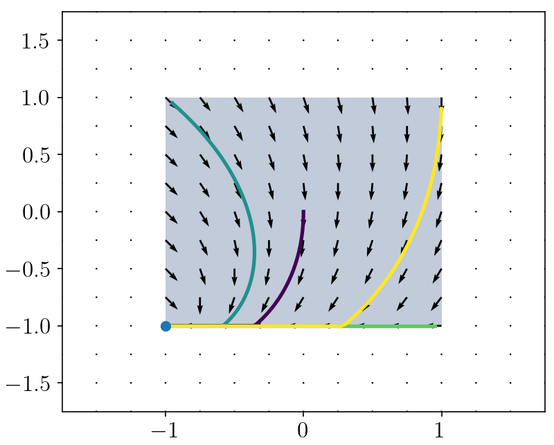
(a) Projected monotone flow

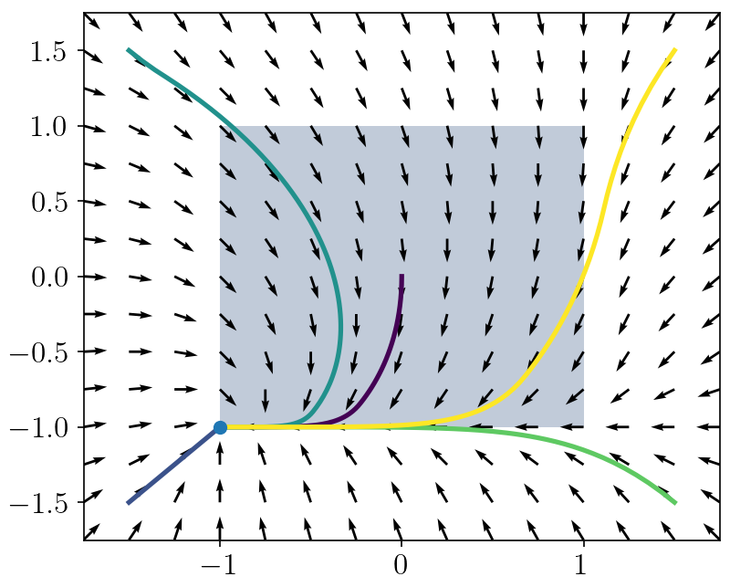
(b) Safe monotone flow

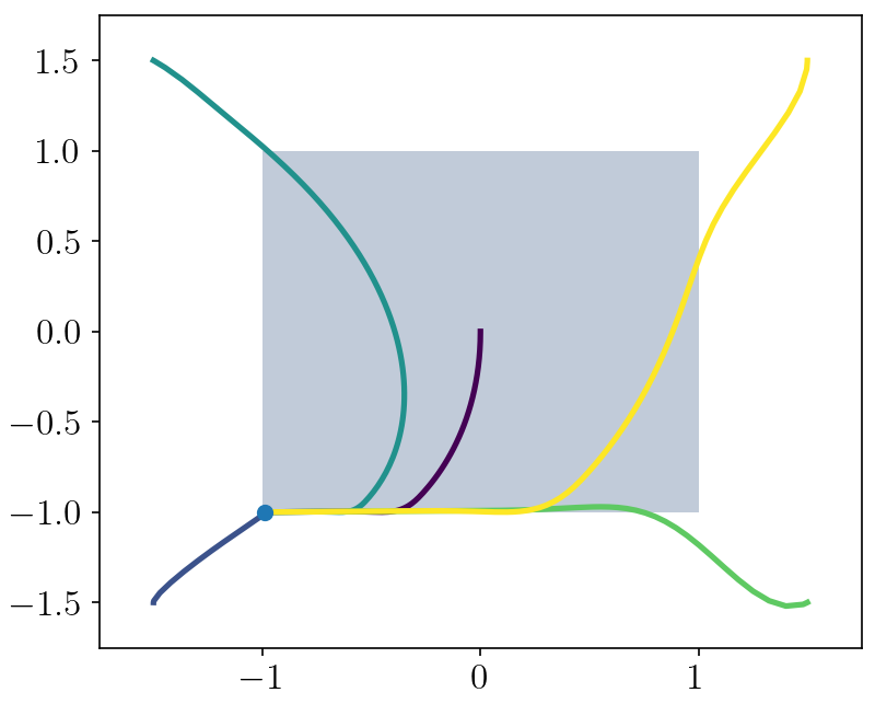
(c) Recursive safe monotone flow

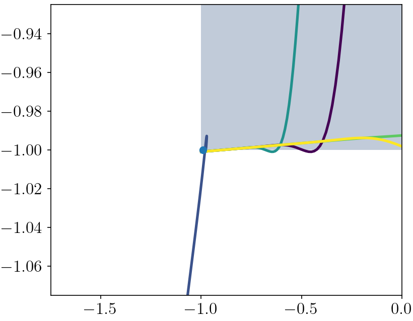
(d) Zoomed-in plot of (c)

Figure 2: Implementation of (a) projected monotone flow, (b) safe monotone flow ($\alpha=1.0$), and (c) recursive safe monotone flow ($\tau=0.25$) in a two-player game. The shaded region shows the constraint set $\mathcal{C}$ and the colored paths represent trajectories of the corresponding flow starting from various initial condition. (d) shows a zoomed-in portion of the boundary of $\mathcal{C}$ to illustrate the practical safety of the recursive safe monotone flow.

7.2 Receding Horizon Linear-Quadratic Dynamic Game

We now discuss a more complex example, where the input to a plant is specified by the solution to a variational inequality parameterized by the state of the plant. To solve it, we interconnect the plant dynamics with the safe monotone flow, and demonstrate that the anytime property of the latter ensures good performance and satisfaction of the constraints even when terminated terminated early. The plant takes the form of a discrete-time linear time-invariant system with two inputs,

$$z(s+1)=Az(s)+B_{1}w_{1}(s)+B_{2}w_{2}(s),$$ (41)

where $A\in^{n_{z}\times n_{z}}$ and $B_{i}\in^{n_{z}\times n_{w}}$ for $i\in\{1,2\}$. We consider a linear-quadratic dynamic game (LQDG) between two players, where each player $i\in\{1,2\}$ can influence the system (41) by choosing the corresponding input $w_{i}\in W_{i}\subset^{n_{w}}$. We fix a time horizon, $N>0$, and an initial condition $z(0)=z_{0}$, and define a cost $J$ as the quadratic payoff function,

$$J(w_{1}(\cdot), w_{2}(\cdot))=\left\lVert z(N)\right\rVert^{2}_{Q_{f}}$$ (42)

$$+\sum_{s=0}^{N-1}\left\lVert z(s)\right\rVert^{2}_{Q}+\left\lVert w_{1}(s)\right\rVert_{R_{1}}^{2}-\left\lVert w_{2}(s)\right\rVert_{R_{2}}^{2},$$

where $Q_{f},Q\succeq 0$ and $R_{1},R_{2}\succ 0$. The goal of player 1 is to minimize the payoff (42), whereas the goal of player 2 is to maximize it. This problem can be solved in closed form when the constraints $W_{i}$ are trivial (cf. [9, Chapter 6], [37]), but must be solved numerically for nontrivial ones.

We first note the LQDG problem can be written as a variational inequality. Indeed, let $\bar{z}=(z(1),\dots,z(N))$ and, for $i\in\{1,2\}$, let $\bar{w}_{i}=(w_{i}(0),\dots,w_{i}(N-1))$. Define

$$\mathcal{A}=\begin{bmatrix}A\\ A^{2}\\ \vdots\\ A^{N}\end{bmatrix},\qquad C_{i}=\begin{bmatrix}B_{i}&0&\cdots&0\\ AB_{i}&B_{i}&\cdots&0\\ A^{2}B_{i}&AB_{i}&\cdots&0\\ \vdots&\vdots&\ddots&\vdots\\ A^{N-1}B_{i}&A^{N-2}B_{i}&\cdots&B_{i}\end{bmatrix}.$$

Next, letting $\bar{Q}=\text{diag}(Q,\dots,Q,Q_{f})$ and $\bar{R}_{i}=\text{diag}(R_{i},\dots,R_{i})$, and using the fact that $\bar{z}=\mathcal{A}z_{0}+C_{1}\bar{w}_{1}+C_{2}\bar{w}_{2}$, we see that the payoff function (42) can be written as,

$$J(\bar{w}_{1},\bar{w}_{2})= \begin{bmatrix}\bar{w}_{1}\\ \bar{w}_{2}\end{bmatrix}^{\top}\begin{bmatrix}C_{1}^{\top}\bar{Q}C_{1}+\bar{R}_{1}&C_{1}^{\top}\bar{Q}C_{2}\\ C_{2}^{\top}\bar{Q}C_{1}&C_{2}^{\top}\bar{Q}C_{2}-\bar{R}_{2}\end{bmatrix}\begin{bmatrix}\bar{w}_{1}\\ \bar{w}_{2}\end{bmatrix}$$

$$+2\begin{bmatrix}C_{1}^{\top}\bar{Q}\mathcal{A}z_{0}\\ C_{2}^{\top}\bar{Q}\mathcal{A}z_{0}\end{bmatrix}^{\top}\begin{bmatrix}\bar{w}_{1}\\ \bar{w}_{2}\end{bmatrix}+z_{0}^{\top}\mathcal{A}^{\top}\bar{Q}\mathcal{A}z_{0}.$$

Finally, letting $x=(\bar{w}_{1},\bar{w}_{2})$, we see that the problem corresponds to the variational inequality $\textnormal{VI}(F(\cdot,z_{0}),\mathcal{C})$, where

$$F(x,z_{0})\!=\!\begin{bmatrix}C_{1}^{\top}\bar{Q}C_{1}+\bar{R}_{1}&C_{1}^{\top}\bar{Q}C_{2}\\ -C_{2}^{\top}\bar{Q}C_{1}&\bar{R}_{2}-C_{2}^{\top}\bar{Q}C_{2}\end{bmatrix}\!\begin{bmatrix}\bar{w}_{1}\\ \bar{w}_{2}\end{bmatrix}\!+\!\begin{bmatrix}C_{1}^{\top}\bar{Q}\mathcal{A}z_{0}\\ -C_{2}^{\top}\bar{Q}\mathcal{A}z_{0}\end{bmatrix}$$

and the constraint set is

$$\mathcal{C}=\underset{N\text{ times}}{\underbrace{W_{1}\times W_{1}\times\cdots W_{1}}}\times\underset{N\text{ times}}{\underbrace{W_{2}\times W_{2}\times\cdots\times W_{2}}}.$$

If the problem data satisfies

$$\begin{bmatrix}C_{1}^{\top}\bar{Q}C_{1}+\bar{R}_{1}&0\\ 0&\bar{R}_{2}-C_{2}^{\top}\bar{Q}C_{2}\end{bmatrix}\succ 0,$$

then $F$ is strongly monotone.

For simulation purposes, we take $n_{z}=5$, $n_{w}=2$, $B_{i}=I$, $W_{i}=^{2}_{\geq 0}$, and $A$ a marginally stable matrix selected randomly. We use the safe monotone flow to solve the variational inequality and implement the solution in a receding horizon manner: given the initial state $z_{0}$, we solve for the optimal input sequence $(w_{1}(\cdot),w_{2}(\cdot))$ over the entire time horizon, apply the input $(w_{1}(0),w_{2}(0))$ to (41) to obtain $z(1)$, update the initial condition $z_{0}\leftarrow z(1)$ and repeat. When $F$ is strongly monotone, on each iteration the flow converges to the exact solution as $t\to\infty$. However, we also consider here the effect of terminating the solver early at some $t=t_{f}<\infty$.

Figure 3 shows the results of the simulation. In Figure 3(a), we plot $\left\lVert z(s)\right\rVert$ for various values of termination times. We denote the exact solution with $t_{f}=\infty$. The closed-loop dynamics with the exact solution to the receding horizon LQDG is stabilizing, and as $t_{f}$ grows larger, the early terminated solution drives the state of the system closer to the origin. In Figure 3(b), we plot the first component of $w_{1}(s)$ in blue and the first component of $w_{2}(s)$ in red. Regardless of when terminated, the inputs satisfy the input constraints on each iteration due to the safety properties of the safe monotone flow.

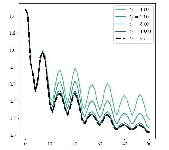
(a) $\left\lVert z(s)\right\rVert$ on each iteration

(b) First component of $\{w_{i}(s)\}_{i\in\{1,2\}}$ on each iteration

Figure 3: Receding horizon implementation of the safe monotone flow solving a linear quadratic dynamic game for different choices of termination time $t_{f}$. The closed-loop implementation of the exact solution corresponds to $t_{f}=\infty$ (dashed lines). (a) We plot the evolution of $\left\lVert z(s)\right\rVert$ in green. (b) We plot the evolution of the first component of $w_{1}(s)$ in blue-green (scale in left $y$-axis) and the first component of $w_{2}(x)$ in red-orange (scale in right $y$-axis).

8 Conclusions

We have tackled the design of anytime algorithms to solve variational inequalities as a feedback control problem. Using techniques from safety-critical control, we have synthesized three continuous-time dynamics which find solutions to monotone variational inequalities: the projected monotone flow, already well known in the literature, and the novel safe monotone and recursive safe monotone flows. The equilibria of these flows correspond to solutions of the variational inequality, and so we have embarked in the precise characterization of their asymptotic stability properties. We have established asymptotic stability of equilibria in the case of strong monotonicity, and contractivity and exponential stability in the case of polyhedral constraints. We have also shown that the safe monotone flow renders the constraint forward invariant and asymptotically stable. The recursive safe monotone flow offers an alternative implementation that does not necessitate the solution of a quadratic program along the trajectories. This flow results from coupling two systems evolving on different timescales, and we have established local exponential stability and global attractivity of equilibria, as well as practical safety guarantees. We have illustrated in two game scenarios the properties of the proposed flows and, in particular, their amenability for interconnection and regulation of physical processes. Future work will develop methods for distributed network problems and consider applications to feedback optimization arising in applications such as power systems, traffic networks, and communications systems.

References

- [1] A. Agarwal, J. W. Simpson-Porco, and L. Pavel. Game-theoretic feedback-based optimization. IFAC-PapersOnLine, 55(13):174–179, 2022.
- [2] A. Allibhoy and J. Cortés. Safety-critical control as a design paradigm of anytime solvers of variational inequalities. In IEEE Conf. on Decision and Control, pages 6211–6216, Cancun, Mexico, December 2022.
- [3] A. Allibhoy and J. Cortés. Control barrier function-based design of gradient flows for constrained nonlinear programming. IEEE Transactions on Automatic Control, 69(6), 2024. To appear.
- [4] A. D. Ames, S. Coogan, M. Egerstedt, G. Notomista, K. Sreenath, and P. Tabuada. Control barrier functions: theory and applications. In European Control Conference, pages 3420–3431, Naples, Italy, 2019.
- [5] A. D. Ames, X. Xu, J. W. Grizzle, and P. Tabuada. Control barrier function based quadratic programs for safety critical systems. IEEE Transactions on Automatic Control, 62(8):3861–3876, 2017.
- [6] K. B. Ariyur and M. Krstić. Real-Time Optimization by Extremum-Seeking Control. Wiley, New York, 2003.
- [7] K. Arrow, L Hurwitz, and H. Uzawa. Studies in Linear and Non-Linear Programming. Stanford University Press, Stanford, CA, 1958.
- [8] J. P. Aubin and A. Cellina. Differential Inclusions, volume 264 of Grundlehren der mathematischen Wissenschaften. Springer, New York, 1984.
- [9] T. Başar and G. J. Olsder. Dynamic Noncooperative Game Theory. SIAM, 2 edition, 1999.
- [10] G. Belgioioso, D. Liao-McPherson, M. H. de Badyn, S. Bolognani, R. S. Smith, J. Lygeros, and F. Dörfler. Online feedback equilibrium seeking. arXiv preprint arXiv:2210.12088, 2022.
- [11] G. Bianchin, J. Cortés, J. I. Poveda, and E. Dall’Anese. Time-varying optimization of LTI systems via projected primal-dual gradient flows. IEEE Transactions on Control of Network Systems, 9(1):474–486, 2022.
- [12] F. Blanchini. Set invariance in control. Automatica, 35(11):1747–1767, 1999.
- [13] V. Bondarevsky, A. Leschov, and L. Minchenko. Value functions and their directional derivatives in parametric nonlinear programming. Journal of Optimization Theory & Applications, 171(2):440–464, 2016.
- [14] S. Boyd and L. Vandenberghe. Convex Optimization. Cambridge University Press, Cambridge, UK, 2009.
- [15] Haim Brezis. Operateurs Maximaux Monotones et Semi-groupes de Contractions dans Les Espaces de Hilbert. Elsevier, 1973.
- [16] R. W. Brockett. Dynamical systems that sort lists, diagonalize matrices, and solve linear programming problems. Linear Algebra and its Applications, 146:79–91, 1991.
- [17] B. Brogliato, A. Daniilidis, C. Lemaréchal, and V. Acary. On the equivalence between complementarity systems, projected systems, and differential inclusions. Systems & Control Letters, 55(1):45–51, 2006.
- [18] F. Bullo. Contraction Theory for Dynamical Systems. Kindle Direct Publishing, 1.1 edition, 2023.
- [19] M. Cohen and C. Belta. Adaptive and Learning-Based Control of Safety-Critical Systems. Springer, New York, 2023.
- [20] M. Colombino, E. Dall’Anese, and A. Bernstein. Online optimization as a feedback controller: Stability and tracking. IEEE Transactions on Control of Network Systems, 7(1):422–432, 2020.
- [21] J. Cortés. Discontinuous dynamical systems - a tutorial on solutions, nonsmooth analysis, and stability. IEEE Control Systems, 28(3):36–73, 2008.
- [22] L. Cothren, F. Bullo, and E. Dall’Anese. Singular perturbation via contraction theory. arXiv preprint arXiv:2310.07966, 2023.
- [23] E. Dall’Anese and A. Simonetto. Optimal power flow pursuit. IEEE Transactions on Smart Grid, 9(2):942–952, 2016.
- [24] A. Davydov, S. Jafarpour, and F. Bullo. Non-Euclidean contraction theory for robust nonlinear stability. IEEE Transactions on Automatic Control, 67(12):6667–6681, 2022.
- [25] G. Delimpaltadakis and W. P. M. H. Heemels. On the relationship between control barrier functions and projected dynamical systems. arXiv preprint arXiv:2309.04378, 2023.
- [26] G. Di Pillo and L. Grippo. Exact penalty functions in constrained optimization. SIAM Journal on Control and Optimization, 27(6):1333–1360, 1989.
- [27] F. Facchinei and J.-S. Pang. Finite-Dimensional Variational Inequalities and Complementarity Problems. Springer, 2003.
- [28] P. Frihauf, M. Krstić, and T. Başar. Nash equilibrium seeking in noncooperative games. IEEE Transactions on Automatic Control, 57(5):1192–1207, 2012.
- [29] A. Hauswirth, S. Bolognani, G. Hug, and F. Dörfler. Optimization algorithms as robust feedback controllers. arXiv preprint arXiv:2103.11329, 2021.
- [30] W. P. M. H. Heemels, J. M. Schumacher, and S. Weiland. Projected dynamical systems in a complementarity formalism. Operations Research Letters, 27:83–91, 2000.
- [31] U. Helmke and J. B. Moore. Optimization and Dynamical Systems. Springer, 1994.
- [32] S. Kolathaya and A. D. Ames. Input-to-state safety with control barrier functions. IEEE Control Systems Letters, 3(1):108–113, 2018.
- [33] L. S. P. Lawrence, J. W. Simpson-Porco, and E. Mallada. Linear-convex optimal steady-state control. IEEE Transactions on Automatic Control, 66(11):5377–5384, 2021.
- [34] J. Liu. Sensitivity analysis in nonlinear programs and variational inequalities via continuous selections. 33(4):1040–1060, 1995.
- [35] S. H. Low, F. Paganini, and J. C. Doyle. Internet congestion control. IEEE Control Systems, 22(1):28–43, 2002.
- [36] A. Nagurney and D. Zhang. Projected Dynamical Systems and Variational Inequalities with Applications, volume 2 of International Series in Operations Research and Management Science. Kluwer Academic Publishers, Dordrecht, The Netherlands, 1996.
- [37] M. Pachter and K. D. Pham. Discrete-time linear-quadratic dynamic games. Journal of Optimization Theory & Applications, 146:151–179, 2010.
- [38] S. M. Robinson. Stability theory for systems of inequalities. Part I: Linear systems. SIAM Journal on Numerical Analysis, 12(5):754–769, 1975.
- [39] R. T. Rockafellar. Convex Analysis. Princeton University Press, 1970.
- [40] R. T. Rockafellar and R. J. B. Wets. Variational Analysis, volume 317 of Comprehensive Studies in Mathematics. Springer, New York, 1998.
- [41] H. L. Royden and P. Fitzpatrick. Real Analysis. Prentice Hall, 2010.
- [42] P. Wieland and F. Allgöwer. Constructive safety using control barrier functions. IFAC Proceedings Volumes, 40(12):462–467, 2007.
- [43] A. Williams, M. Krstic, and A. Scheinker. Semi-global practical extremum seeking with practical safety. arXiv preprint arXiv:2309.15401, 2023.
- [44] W. Xiao, C. G. Cassandras, and C. Belta. Safe Autonomy with Control Barrier Functions: Theory and Applications. Synthesis Lectures on Computer Science. Springer, New York, 2023.
- [45] N. D. Yen. Lipschitz continuity of solutions of variational inequalities with a parametric polyhedral constraint. Mathematics of Operations Research, 20(3):695–708, 1995.