Identifying Systems with Symmetries using Equivariant Autoregressive Reservoir Computers

Abstract

The investigation reported in this document focuses on identifying systems with symmetries using equivariant autoregressive reservoir computers. General results in structured matrix approximation theory are presented, exploring a two-fold approach. Firstly, a comprehensive examination of generic symmetry-preserving nonlinear time delay embedding is conducted. This involves analyzing time series data sampled from an equivariant system under study. Secondly, sparse least-squares methods are applied to discern approximate representations of the output coupling matrices. These matrices play a pivotal role in determining the nonlinear autoregressive representation of an equivariant system. The structural characteristics of these matrices are dictated by the set of symmetries inherent in the system. The document outlines prototypical algorithms derived from the described techniques, offering insight into their practical applications. Emphasis is placed on their effectiveness in the identification and predictive simulation of equivariant nonlinear systems.

1 Introduction

In the dynamic realm of computational science, reservoir computing has emerged as a formidable approach for system identification and dynamic modeling. Notably, this machine learning algorithm excels in processing information from dynamical systems using observed time-series data, primarily due to its minimal training data and computational resource requirements. Yet, the traditional reservoir computing model, reliant on randomly sampled matrices for its underlying recurrent neural network, faces challenges from the numerous metaparameters needing optimization. Recent strides, particularly in nonlinear vector autoregression (NVAR), have marked a significant evolution in reservoir computing by offering efficient alternatives requiring shorter training datasets and less training time Gauthier et al. (2021).

Building upon these advancements, this paper introduces an extended autoregressive reservoir computing strategy, tailored for modeling dynamic systems with inherent symmetries. Our work delves into the theoretical underpinnings and algorithmic strategies crucial for realizing these novel reservoir computing architectures. These architectures not only reflect linear and nonlinear autoregressive vector models but also incorporate symmetry-preserving equivariant matrix approximation methods, thereby offering a nuanced approach to equivariant system identification and modeling.

Our investigation presents as a main contribution: a strategy that bridges structured matrix approximation methods with the robustness of autoregressive models. This synergetic approach, detailed in Section 3, provides a reliable mathematical solution for identifying dynamic systems with symmetries accurately and efficiently.

A particularly exciting offshoot of our research is the development of a Python-based toolkit for equivariant reservoir computer model identification. This toolkit embodies the practical application of concepts discussed in Sections 3 and 4, and is readily accessible for scholarly use.

The practical implications of our structured operator identification technology are vast and varied, with applications stretching from the nuanced demands of cyber-physical systems simulation Yuan et al. (2019) to toxicity prediction Cremer et al. (2023).

To demonstrate the practical application of the proposed theory, we present a prototype algorithm for the computation of equivariant autoregressive reservoir computers, rooted in the methodologies expounded upon in Section 3. This is further brought to life in Section 4, where we outline the algorithm’s architecture and functionality.

Finally, in Section 5, we present two computational experiments. The first experiment is focused on the identification of a Hamiltonian system that is characterized by its inherent symmetries. The second experiment applies the symmetry-preserving system identification methods discussed in our study to the realm of finance. Here, we simulate the ”representation ranking” of five financial institutions within a given market or portfolio. Inspired by dynamic ecological models for competitive species, this approach assigns a score ranging from $0$ to $1$ to each institution. The representation ranking measures each institution’s market participation compared to its peers, providing a nuanced view of its financial influence and dominance. Furthermore, this methodology offers potential applications in assessing financial stability, as it captures the dynamic balance similar to that observed in natural systems. Through this, the representation ranking not only reveals the competitive dynamics of each institution but also hints at their broader implications for market stability, reflecting their varying positions over time.

2 Preliminaries and Notation

The symbols $\mathbb{R}^{+}$ and $\mathbb{Z}^{+}$ will be used to denote the positive real numbers and positive integers, respectively. For any pair $p,n\in\mathbb{Z}^{+}$ the expression $d_{p}(n)$ will denote the positive integer $d_{p}(n)=n(n^{p}-1)/(n-1)+1$. For any finite group $G$, the expression $|G|$ will be used to denote the order of $G$, that is, the number of elements of $G$. The symbol $\mathbf{1}_{n}$ will be used to denote the vector in $\mathbb{R}^{n}$ with all of its coordinates equal to $1$.

Given a scalar time series $\Sigma=\{x_{t}\}_{t\geq 1}\subset\mathbb{R}^{n}$, a positive integer $L$ and any $t\geq L$, we will write $\mathbf{x}_{L}(t)$ to denote the vector:

$$\mathbf{x}_{L}(t)=\begin{bmatrix}\mathbf{x}^{(1)}_{L}(t)^{\top}&\mathbf{x}^{(2)}_{L}(t)^{\top}&\cdots&\mathbf{x}^{(n)}_{L}(t)^{\top}\end{bmatrix}^{\top}\in\mathbb{R}^{nL},$$

with

$$\mathbf{x}^{(j)}_{L}(t)=\begin{bmatrix}x^{(j)}_{t-L+1}&x^{(j)}_{t-L+2}&\cdots&x^{(j)}_{t-1}&x^{(j)}_{t}\end{bmatrix}^{\top}\in\mathbb{R}^{L}.$$

for $1\leq j\leq n$, where $x_{j,s}$ denotes the scalar $j$-component of each element $x_{s}$ in the vector time series $\Sigma$, for $s\geq 1$.

The identity matrix in $\mathbb{R}^{n\times n}$ will be denoted by $I_{n}$, and we will write $\hat{e}_{j,n}$ to denote the matrices in $\mathbb{R}^{n\times 1}$ representing the canonical basis of $\mathbb{R}^{n}$ (each $\hat{e}_{j,n}$ corresponds to the $j$-column of $I_{n}$). Given a matrix $X\in\mathbb{R}^{m\times n}$, the expression $\|X\|_{F}$ will denote the Frobenius norm of $X$.

For any integer $n>0$, in this article, we will identify the vectors in $\mathbb{R}^{n}$ with column matrices in $\mathbb{R}^{n\times 1}$.

Given a matrix $A\in\mathbb{R}^{m\times n}$, we write $\mathrm{vec}(A)$ to denote the column vector obtained by stacking the columns of $A$ according to the following expression

$$\mathrm{vec}(A)=\begin{bmatrix}\mathbf{a}[1]^{\top}&\cdots&\mathbf{a}[n]^{\top}\end{bmatrix}^{\top}$$

where $\mathbf{a}[j]$ denotes the $j$-column of $A$ for $1\leq j\leq n$. For any $\mathbf{x}\in\mathbb{R}^{mn}$ we will write $\mathrm{vec}^{\dagger}_{m}(\mathbf{x})$ to denote the operation such that $\mathrm{vec}_{m}^{\dagger}(\mathrm{vec}(A))=A$ for any $A\in\mathbb{R}^{m\times n}$.

Let $A\in\mathbb{R}^{m\times n}$, $B\in\mathbb{R}^{p\times q}$, the tensor Kronecker tensor product $A\otimes B\in\mathbb{R}^{mp\times nq}$ is determined by the following operation.

$$A\otimes B=\begin{bmatrix}a_{11}B&\cdots&a_{1n}B\\ \vdots&\ddots&\vdots\\ a_{m1}B&\cdots&a_{mn}B\end{bmatrix}$$

For any integer $p>0$ and any matrix $X\in\mathbb{R}^{m\times n}$, we will write $X^{\otimes p}$ to denote the operation determined by the following expression.

$$X^{\otimes p}=\left\{\begin{array}[]{ll}X&,p=1\\ X\otimes X^{\otimes(p-1)}&,p\geq 2\end{array}\right.$$

We will also use the symbol $\Pi_{p}$ to denote the operator $\Pi_{p}:\mathbb{R}^{n}\to\mathbb{R}^{n^{p}}$ that is determined by the expression $\Pi_{p}(x):=x^{\otimes p}$, for each $x\in\mathbb{R}^{n}$. Given a list $A_{1},A_{2},\ldots,A_{m}$ such that for $1\leq j\leq m$, $A_{j}\in\mathbb{R}^{n_{j}\times n_{j}}$ for some integer $n_{j}>0$. The expression $A_{1}\oplus A_{2}\oplus\cdots\oplus A_{m}$ will denote the block diagonal matrix

$$A_{1}\oplus A_{2}\oplus\cdots\oplus A_{m}=\begin{bmatrix}A_{1}&&&\\ &A_{2}&&\\ &&\ddots&\\ &&&A_{m}\end{bmatrix},$$

where the zero matrix blocks have been omitted. Given two vectors $\mathbf{x}=[x_{j}]$, $\mathbf{y}$ in $\mathbb{R}^{m}$, we will write $\mathbf{x}\odot\mathbf{y}$ to denote the operation corresponding to their Hadamard product $\mathbf{x}\odot\mathbf{y}=\begin{bmatrix}x_{j}y_{j}\end{bmatrix}\in\mathbb{R}^{m}$. The group of orthogonal matrices in $\mathrm{R}^{n\times n}$ will be denoted by $\mathbb{O}(n)$ in this study.

3 Approximate evolution operator representation

Let us consider discrete-time dynamical systems determined by the pair $(\hat{\boldsymbol{\Sigma}},\mathcal{T})$ with $\hat{\boldsymbol{\Sigma}}\subset\mathbb{R}^{n}$, where $\mathcal{T}:\hat{\boldsymbol{\Sigma}}\to\hat{\boldsymbol{\Sigma}}$ is an evolution operator. Given a finite group $G$ and some matrix representation (Steinberg, 2012, Definition 3.1.1) $\boldsymbol{\pi}:G\to G_{\boldsymbol{\pi}}\subset\mathbb{O}(n),g\mapsto g_{\boldsymbol{\pi}}$, the system $(\hat{\boldsymbol{\Sigma}},\mathcal{T})$ is said to be $G$-equivariant with respect to $\boldsymbol{\pi}$ if:

$$g_{\boldsymbol{\pi}}\mathcal{T}(x)=\mathcal{T}(g_{\boldsymbol{\pi}}x)$$ (1)

for each $x\in\hat{\boldsymbol{\Sigma}}$ and each $g_{\boldsymbol{\pi}}\in\boldsymbol{\pi}(G)$. When it is clear from the context, an explicit reference to $\boldsymbol{\pi}$ may be omitted.

Given $\epsilon>0$, some matrix representation $G_{\boldsymbol{\pi}}\subset\mathbb{O}(n)$ of a finite group $G$, and an orbit of a $G$-equivariant discrete-time system to be identified that can be represented by a vector times series $\Sigma=\{x_{t}\}_{t\geq 1}\subset\mathbb{R}^{n}$. We will study the problem of identifying a (generally nonlinear) operator $\hat{\mathcal{T}}:\mathbb{R}^{n}\to\mathbb{R}^{n}$ such that

$$gx_{t+1}=\hat{\mathcal{T}}(gx_{t}),$$ (2)

for each $1\leq t\leq\tau$, each $g\in G_{\boldsymbol{\pi}}$ and some prescribed $\tau>0$, with $x_{t+1}=\hat{\mathcal{T}}(x_{t})$ for each $t\geq 1$.

3.1 Equivariant reservoir computers for approximate evolution operator representation

When for a matrix representation $\boldsymbol{\pi}:G\to\mathbb{O}(n)$ of some given finite group $G$, we consider the time series data $\Sigma\subset\mathbb{R}^{n}$ corresponding to an orbit determined by the difference equation

$$x_{t+1}=\mathcal{T}(x_{t}),$$ (3)

for some $G$-equivariant discrete-time system $(\hat{\boldsymbol{\Sigma}},\mathcal{T})$ with respect to $\boldsymbol{\pi}$ to be identified. One may need to preprocess the time series data before proceeding with the approximate representation of a suitable evolution operator. For this purpose, given some prescribed integer $L>0$, one can consider the time series $\mathcal{D}_{L}(\Sigma)$ determined by the expression.

$$\mathcal{D}_{L}(\Sigma)=\{\mathbf{x}_{L}(t)\}_{t\geq L}$$

For the dilated time series $\mathcal{D}_{L}(\Sigma)$, the previously considered recurrence relation $x_{t+1}=\mathcal{T}(x_{t})$, $t\geq 1$, induces the following difference equations

$$\mathbf{x}_{L}(t+1)=\tilde{\mathcal{T}}(\mathbf{x}_{L}(t)),$$ (4)

for $t\geq L$. Where $\tilde{\mathcal{T}}$ is some evolution operator to be identified such that

$$(\boldsymbol{\pi}(g)\otimes I_{L})\mathbf{x}_{L}(t+1)=\tilde{\mathcal{T}}\left((\boldsymbol{\pi}(g)\otimes I_{L})\mathbf{x}_{L}(t)\right),$$ (5)

for each $g\in G$.

For any $p\geq 1$, let us consider the map $\eth_{p}:\mathbb{R}^{n}\to\mathbb{R}^{d_{p}(n)}$ for $d_{p}(n)=n(n^{p}-1)/(n-1)+1$, which is determined by the expression.

$$\eth_{p}(x):=\begin{bmatrix}\Pi_{1}(x)\\ \Pi_{2}(x)\\ \vdots\\ \Pi_{p}(x)\\ 1\end{bmatrix}=\begin{bmatrix}x^{\otimes 1}\\ x^{\otimes 2}\\ \vdots\\ x^{\otimes p}\\ 1\end{bmatrix}$$ (6)

Here, the number $p$ will be called the order of the embedding map $\eth_{p}$. Given integers $p,L>0$, an orbit $\Sigma=\{x_{t}\}_{t\geq 1}\subset\mathbb{R}^{n}$ of an equivariant system with a finite symmetry group represented by a set of orthogonal matrices $G\subset\mathbb{R}^{n\times n}$. For a finite sample $\Sigma_{N}=\{x_{t}\}_{t=1}^{T}\subset\Sigma$, let us consider the matrices:

$$\mathbf{H}^{(0,p)}_{L}(\Sigma_{T}) =\begin{bmatrix}\eth_{p}(\mathbf{x}_{L}(L))&\cdots&\eth_{p}(\mathbf{x}_{L}(T-1))\end{bmatrix}$$ (7)

$$\mathbf{H}^{(1)}_{L}(\Sigma_{T}) =\begin{bmatrix}\mathbf{x}_{L}(L+1)&\cdots&\mathbf{x}_{L}(T)\end{bmatrix}$$

The operator identification mechanism used in this study for dilated systems of the form (4), will be described by the expression:

$$\hat{\mathcal{T}}(\mathbf{x}_{L}(t))=W\eth_{p}(\mathbf{x}_{L}(t)),\>\>t\geq L,$$ (8)

for some matrix $W=\hat{W}R_{p,L}(n)\in\mathbb{R}^{n\times d_{p}(n)}$ to be partially determined, with $d_{p}(n)=n(n^{p}-1)/(n-1)+1$. Building on the operator theoretic techniques and ideas presented in Rieffel (1980), Maehara and Murota (2011), Panahi et al. (2021) and Vides et al. (2023), the matrix $\hat{W}$ in (8) can be estimated by approximately solving the matrix equation

$$\hat{W}(R_{p,L}(n)\mathbf{H}^{(0,p)}_{L}(\Sigma_{T}))=\mathbf{H}^{(1)}_{L}(\Sigma_{T}).$$ (9)

Where $R_{p,L}(n)$ is the matrix described by (Vides et al., 2023, Theorem III.6), and by (4) and (5) $\hat{W}$ shall belong to the linear space of matrices that solve equations of the form:

$$\|g_{j}\otimes I_{L}X-XR_{p,L}(n)G_{j}\|_{F}=0,1\leq j\leq|\mathbf{G}_{\boldsymbol{\pi}}|$$ (10)

and where for each $1\leq j\leq|\mathbf{G}_{\boldsymbol{\pi}}|$ the matrix $G_{j}$ satisfies the condition

$$\eth_{p}(g_{j}\otimes I_{L}\mathbf{x})=G_{j}\eth_{p}(\mathbf{x})$$ (11)

for any $\mathbf{x}\in\mathbb{R}^{nL}$. The devices described by (8) are called equivariant autoregressive reservoir computers (EARC) in this paper.

3.2 Structured output coupling matrix identification

The solvability of the matrix identification problems described by equations (10) and (11) will be studied from a structured matrix analysis perspective.

Lemma 1

Given an integer $p\geq 1$, and a finite group representation $\mathbf{G}_{\boldsymbol{\pi}}=\{g_{1},\ldots,g_{N}\}\subset\mathbb{O}(n)$. For each $1\leq j\leq N=|\mathbf{G}_{\boldsymbol{\pi}}|$, the matrix $G_{j}$ satisfies the condition

$$\eth_{p}(g_{j}\otimes I_{L}\mathbf{x})=G_{j}\eth_{p}(\mathbf{x})$$

for any $\mathbf{x}\in\mathbb{R}^{nL}$, is determined by the expression

$$G_{j}:=(g_{j}\otimes I_{L})\oplus(g_{j}\otimes I_{L})^{\otimes 2}\oplus\cdots\oplus(g_{j}\otimes I_{L})^{\otimes p}\oplus 1.$$ (12)

By iterating on (Zhan, 2013, Lemma 2.1) we will have that for any $\mathbf{x}\in\mathbb{R}^{nL}$ and any integers $k\geq 1$ and $1\leq j\leq N$:

$$((g_{j}\otimes I_{L})\mathbf{x})^{\otimes k} =(g_{j}\otimes I_{L})^{\otimes k}\mathbf{x}^{\otimes k}$$

$$=(g_{j}\otimes I_{L})^{\otimes k}\Pi_{k}(\mathbf{x})$$

Consequently, by (6) it can be seen that if $G_{j}$ is determined by (12) we will have that

$$\eth_{p}(g_{j}\otimes I_{L}\mathbf{x})=G_{j}\eth_{p}(\mathbf{x}).$$

This completes the proof.

Given a finite group representation $\mathbf{G}_{\boldsymbol{\pi}}=\{g_{1},\ldots,g_{N}\}\subset\mathbb{O}(n)$ and a subset of matrix representations $\{\hat{g}_{1},\ldots,\hat{g}_{r}\}\subset\mathbf{G}_{\boldsymbol{\pi}}$ of the generators of $G$, then a basis for the space of solutions to equations (10) can be computed by applying the following lemma.

Lemma 2

Given a subset of matrix representations $\{\hat{g}_{1}$ , $\ldots$ , $\hat{g}_{r}\}$ $\subset$ $\mathbf{G}_{\boldsymbol{\pi}}$ of the generators of a group of symmetries $G$ of a $G$-equivariant system under study whose output coupling matrix is determined by (9), then a basis $\{X_{1},\ldots,X_{M}\}$ for the space of solutions to equations (10) will be determined by a basis $\{\mathbf{x}_{1},\ldots,\mathbf{x}_{M}\}$ of

$$\ker\left(\sum_{j=1}^{r}K_{j}^{\top}K_{j}\right)$$ (13)

according to the rule

$$X_{j}=\mathrm{vec}_{nL}^{\dagger}(\mathbf{x}_{j}),1\leq j\leq M.$$ (14)

Where

$$K_{j}:=I_{q_{1}}\otimes(\hat{g}_{j}\otimes I_{L})-(G_{j}^{\top}R_{p,L}(n)^{\top})\otimes I_{q_{2}}$$ (15)

for each $1\leq j\leq r$ and some suitable integers $q_{1},q_{2}\geq 1$.

Let $q_{1}=nL$ and $q_{2}$ be equal to the number of rows of $R_{p,L}(n)$ determined by (Vides et al., 2023, Theorem III.6). Since $\hat{g_{1}},\ldots,\hat{g}_{r}$ represent generators of the group of symmetries $G$, by (Zhan, 2013, Equation (2.10) in §2.2), (15), and by matrix kernel properties we will have that any matrix solvent $X$ of the matrix equations (10) satisfies the following condition.

$$\mathrm{vec}(X)\in\ker\left(\begin{bmatrix}K_{1}\\ \vdots\\ K_{r}\end{bmatrix}\right)=\ker\left(\sum_{j=1}^{r}K_{j}^{\top}K_{j}\right)$$ (16)

Consequently, given a basis $\{\mathbf{x}_{1},\ldots,\mathbf{x}_{M}\}$ (13) we will have that $\mathrm{vec}(X)\in\mathrm{span}(\{\mathbf{x}_{1},\ldots,\mathbf{x}_{M}\})$. Therefore, $X\in\mathrm{span}(\{\mathrm{vec}_{nL}^{\dagger}(\mathbf{x}_{1}),\ldots,\mathrm{vec}_{nL}^{\dagger}(\mathbf{x}_{M})\})$ and $\{\mathrm{vec}_{nL}^{\dagger}(\mathbf{x}_{1})$ , $\ldots$ , $\mathrm{vec}_{nL}^{\dagger}(\mathbf{x}_{M})\}$ determines a basis for the space of solutions to (10). This completes the proof.

Corollary 3

Let us consider the matrix equation (9), and let us set:

$$\mathbf{H}_{0} :=R_{p,L}(n)\mathbf{H}^{(0,p)}_{L}(\Sigma_{T}),$$

$$\mathbf{H}_{1} :=\mathbf{H}^{(1)}_{L}(\Sigma_{T}).$$

A structured output coupling matrix $\hat{W}$ that satisfies (9) and (10), can be identified using the expression

$$\hat{W}:=\sum_{j=1}^{m}c_{j}X_{j}.$$

Where $\{X_{1},\ldots,X_{M}\}$ is the basis for the space of solutions to equations (10) described by Lemma 2, and the coefficients $c_{j}$ can be obtained by solving the following linear system of equations

$$\begin{bmatrix}|&&|\\ \mathrm{vec}(X_{1}\mathbf{H}_{0})&\cdots&\mathrm{vec}(X_{M}\mathbf{H}_{0})\\ |&&|\end{bmatrix}\begin{bmatrix}c_{1}\\ \vdots\\ c_{M}\end{bmatrix}=\mathrm{vec}(\mathbf{H}_{1}).$$ (17)

This is can be verified by applying the operation $\mathrm{vec}$ to both sides of (9), and is a consequence of linear space bases properties and the definition of the operation $\mathrm{vec}$, as it can be seen from its definition of this operation that the operation $\mathrm{vec}$ is linear. This completes the proof.

4 Algorithm

In this section, we focus on the applications of the structured matrix approximation methods presented in §3, to reservoir computer models identification for equivariant dynamical systems. More specifically, we propose a prototypical algorithm for general purpose equivariant system identification, that is described by Algorithm 1.

Data: $\Sigma_{T}=\{x_{t}\}_{t=1}^{T}\subset\mathbb{R}^{n},\mathbf{G}_{\boldsymbol{\pi}}\subset\mathbb{O}(n)$.

Result: $\hat{W},R_{p,L}(n)$

• Choose or estimate the lag value $L$ using auto-correlation function based methods.

• Set a tensor order value $p$.

• Compute compression matrix $R_{p,L}(n)$ applying Algorithm A.2 in Vides et al. (2023).

• Compute matrices:

  $$\mathbf{H}_{0} :=\mathbf{H}^{(0,p)}_{L}(\Sigma_{T})$$

  $$\mathbf{H}_{1} :=\mathbf{H}^{(1)}_{L}(\Sigma_{T})$$

• For each $g_{j}\in\mathbf{G}_{\boldsymbol{\pi}}$, compute the matrix $G_{j}$ such that $\eth_{p}(g_{j}\otimes I_{L}\mathbf{x})=G_{j}\eth_{p}(\mathbf{x})$ for any $\mathbf{x}\in\mathbb{R}^{nL}$.

• Compute a basis $\{\hat{X}_{1},\ldots,\hat{X}_{m}\}$ for the space of solutions to equations:

  $$g_{j}\otimes I_{L}X-XR_{p,L}(n)G_{j}=\mathbf{0}_{n},1\leq j\leq|\mathbf{G}_{\boldsymbol{\pi}}|$$

• Compute the coefficients that approximately solve:

  $$\sum_{j=1}^{m}c_{j}\hat{X}_{j}\left(R_{p,L}(n)\mathbf{H}_{0}\right)=\mathbf{H}_{1}$$

  applying Algorithm A.1 in Vides et al. (2023).

• Set $\hat{W}:=\sum_{j=1}^{m}c_{j}\hat{X}_{j}$.

return $\hat{W},R_{p,L}(n)$

Algorithm 1 EARCModel: EARC model identification

5 Computational Examples

In this section we will present some numerical simulations computed using the SPORT toolset available in Vides (2023), which was developed as part of this project, the toolset consists of a collection of programs written in Python that can be used for sparse identification and numerical simulation of dynamical systems.

The numerical experiments documented in this section were performed with Python 3.8.10. All the programs written for synthetic data generation and sparse model identification as part of this project are available at Vides (2023).

5.1 Identification of a Hamiltonian system with symmetries using EARC

Let us consider a Hamiltonian system determined by the following initial value problem.

$$\frac{dq}{dt}=p^{3}-p,$$ (18)

$$\frac{dp}{dt}=q^{3}-q,$$

$$q(0)=1,p(0)=0$$

As observed in (Sinha et al., 2020) the system (18) is $K_{4}$-equivariant. For the configuration used for this experiment, the matrix representation $\mathbf{G}_{\boldsymbol{\pi}}(K_{4})$ of the corresponding group of symmetries

$$K_{4}=\left\langle r_{1},r_{2}\left|r_{1}^{2}=r_{2}^{2}=\left(r_{1}r_{2}\right)^{2}=e\right.\right\rangle$$

is determined by the following assignments.

$$r_{1} \mapsto r_{1,\boldsymbol{\rho}}=\begin{bmatrix}0&1\\ 1&0\end{bmatrix}$$

$$r_{2} \mapsto r_{2,\boldsymbol{\rho}}=\begin{bmatrix}-1&0\\ 0&-1\end{bmatrix}$$

The synthetic signals corresponding to the data sample $\Sigma_{600}\subset\mathbb{R}^{3}$ that will be used for system identification have been computed with an explicit time integration scheme, using lsoda from the FORTRAN library odepack via the Python function odeint, with the Python program HamiltonianSystem.py in Vides (2023). The model was trained using an embedding map $\eth_{p}$ of order $p=3$, with $15\%$ of the synthetic reference data.

The reference synthetic signal data and the corresponding identified signals are illustrated in Figure 1.

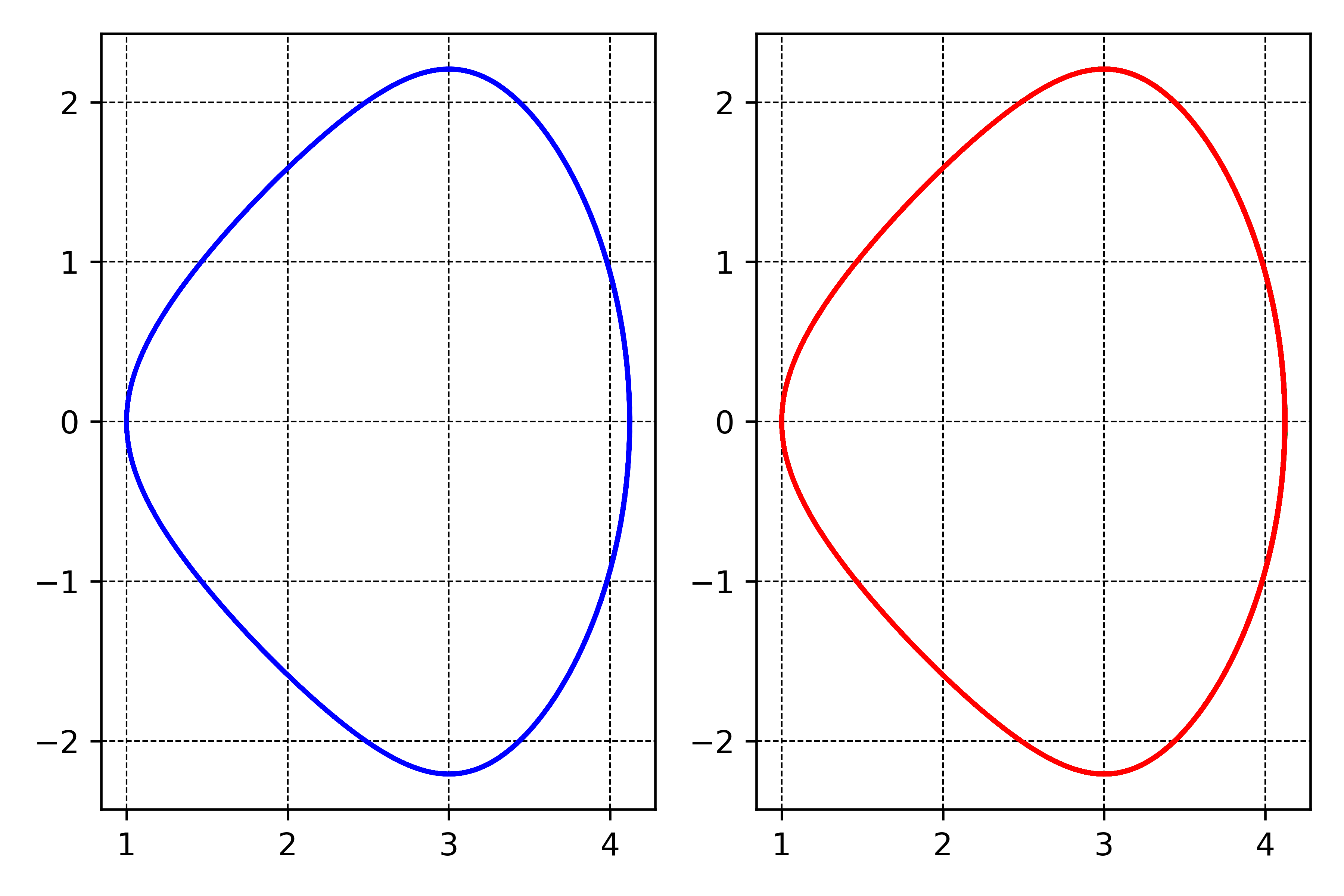
Figure 1: $2D$ graphical representation of: training data (left), predicted behavior (right).

For this experiment we have considered the following configuration: a lag value $L=5$, an embedding order $p=3$. To verify that the output coupling matrix $\hat{W}$ identified for this example using Algorithm 1 satisfies the equivariant matrix constraints (11), we can compute the number:

$$\boldsymbol{\Delta}_{EM}:=\sum_{g_{j}\in\mathbf{G}_{\boldsymbol{\pi}}(K_{4})}\left\|g_{j}\otimes I_{5}\hat{W}R_{3,5}(2)-\hat{W}R_{3,5}(2)G_{j}\right\|_{F}$$

Where each $G_{j}$ is determined by each $g_{j}$ according to (12). For this experiment, we obtain the following value:

$$\boldsymbol{\Delta}_{EM}=4.1434207423062456\times 10^{-15}.$$

The computational setting used for the experiments performed in this section is documented in the Python program HamiltonianSystemID.py in Vides (2023) that can be used to replicate these experiments.

5.2 Identification of a financial competition system with symmetries using EARC

In this experiment, we explore a specific aspect of the commercial banking sub-system, which is part of a larger financial system supervised by a regulatory body. The focus of this study is on the dynamic system that tracks the ”representation ranking” of a selected group of banks. This ranking is a numerical score, ranging from $0$ to $1$, which quantifies each bank’s participation in relation to others within the same market or portfolio. A score of $1$ indicates a leading position in the market or portfolio, while a score of $0$ denotes no market presence.

To compute the representation ranking, we first calculate each bank’s total participation in the market or portfolio under consideration. We then identify the bank or banks with the highest market participation. The participation of each bank is divided by this maximum value, yielding a score between $0$ and $1$. This scoring system ensures that the rankings are consistent and comparable across various markets or portfolios, thereby providing a clear and quantifiable measure of each bank’s relative market dominance and competitive stance.

Furthermore, from the perspective of a regulatory body, the representation ranking model is crucial for assessing financial stability. Banks with higher representation rankings generally are systemically important institutions relevant to the stability of the financial system under consideration. Regulatory bodies can use these models to monitor the market influence and competitive distortions, identify principal peers or competitive groups, and anticipate the accumulation of potential risks. By doing so, they can take proactive measures aimed at preventing and mitigating the impact of failures in banks with higher dominance. In this way, representation ranking serves as a valuable tool for comprehending competitive dynamics and takes on a pivotal role in the development of a proactive regulatory framework that enhances resilience and ensures the overall stability of the financial system.

Let us consider a discrete-time financial competition system for $5$ banks, characterized by the following recurrence relation:

$$\mathbf{p}(t+1)=\mathbf{p}(t)+\mathbf{r}\odot\mathbf{p}(t)\odot(\mathbf{1}_{5}-\mathbf{N}\mathbf{p}(t))$$ (19)

In this model, the $i$-th component $\mathbf{p}(t)[i]$ of each vector $\mathbf{p}(t)$ is an approximate representation for the value at time step $t$, of the discrete-time signal determined by the smoothed evolution of the representation ranking of bank $i$ in a given market or portfolio, as assessed by some regulating body. The matrix $\mathbf{N}$, is defined as:

$$\mathbf{N} =\begin{bmatrix}1&1.1&0&0&1\\ 1&1&1.1&0&0\\ 0&1&1&1.1&0\\ 0&0&1&1&1.1\\ 1.1&0&0&1&1\end{bmatrix}$$

and represents the interaction between banks of the system under consideration. It corresponds to the expected interaction network $\mathcal{N}=(V_{\mathcal{N}},E_{\mathcal{N}})$ of the $5$ banks considered in this experiment. The corresponding directed graph is illustrated in Figure 2.

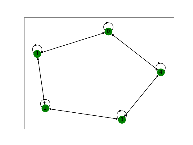
Figure 2: Expected interaction network $\mathcal{N}=(V_{\mathcal{N}},E_{\mathcal{N}})$.

When all components of the growth vector $\mathbf{r}$ are equal, the system becomes $\mathbb{Z}_{5}$-equivariant. For the configuration used for this experiment, $\mathbf{r}=0.376\mathbf{1}_{5}$ and the matrix representation $\mathbf{G}_{\boldsymbol{\pi}}(\mathbb{Z}_{5})$ of the corresponding group of symmetries $\mathbb{Z}_{5}=\langle r|r^{5}=e\rangle$ is determined by the following assignment.

$$r \mapsto r_{\boldsymbol{\rho}}=\begin{bmatrix}0&1&0&0&0\\ 0&0&1&0&0\\ 0&0&0&1&0\\ 0&0&0&0&1\\ 1&0&0&0&0\\ \end{bmatrix}$$

The synthetic signals corresponding to the data sample $\Sigma_{425}\subset\mathbb{R}^{5}$ that will be used for system identification have been computed according to (19). The model was trained using an embedding map $\eth_{p}$ of order $p=2$, with less than $7.3\%$ of the synthetic reference data.

For this experiment, we have considered the following configuration: a lag value $L=1$, and an embedding order $p=2$. To verify that the output coupling matrix $\hat{W}$ identified for this example using Algorithm 1 satisfies the equivariant matrix constraints (11), we can compute the number:

$$\boldsymbol{\Delta}_{EM}:=\sum_{g_{j}\in\mathbf{G}_{\boldsymbol{\pi}}(\mathbb{Z}_{5})}\left\|g_{j}\hat{W}R_{2,1}(5)-\hat{W}R_{2,1}(5)G_{j}\right\|_{F}$$

Where each $G_{j}$ is determined by each $g_{j}$ according to (12). For this experiment, we obtain the following value:

$$\boldsymbol{\Delta}_{EM}=2.083018984548649\times 10^{-14}.$$

The reference synthetic signal data and the corresponding identified signals are illustrated in Figure 3.

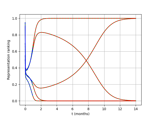
Figure 3: Representation ranking evolution: training data (blue solid lines), reference behavior data (solid green lines), predicted behavior (dashed red lines).

The computational setting used for the experiments performed in this section is documented in the Python program Python program FinancialCompetitionModel.py in Vides (2023) that can be used to replicate these experiments.

6 Data Availability

The Python programs that support the findings of this study are openly available in the SPORT repository, reference number Vides (2023).

7 Conclusion

In conclusion, this study has demonstrated the effectiveness of equivariant autoregressive reservoir computers (EARCs) in identifying systems with inherent symmetries. Our comprehensive analysis revealed that EARCs can successfully capture the underlying dynamics of such systems, preserving their symmetrical properties. The use of sparse least-squares methods further enhanced the ability to discern approximate representations of the output coupling matrices, offering a novel approach to equivariant system identification. These findings not only deepen our understanding of equivariant systems but also open up new possibilities for the application of EARCs in various scientific and engineering domains. This work lays a foundational stone for future research, where the exploration of more complex symmetries and the integration of our methodologies into real-world scenarios could lead to interesting developments in the study and control of dynamical systems with symmetries.

The computational simulations documented in this paper were performed with computational resources from the National Commission of Banks and Insurance Companies of Honduras (CNBS). The views expressed in the article do not necessarily represent the views of the National Commission of Banks and Insurance Companies of Honduras.

References

- Cremer et al. (2023) Cremer, J., Medrano Sandonas, L., Tkatchenko, A., Clevert, D.A., and De Fabritiis, G. (2023). Equivariant graph neural networks for toxicity prediction. Chemical Research in Toxicology, 36(10), 1561–1573. 10.1021/acs.chemrestox.3c00032. URL https://doi.org/10.1021/acs.chemrestox.3c00032.
- Gauthier et al. (2021) Gauthier, D.J., Bollt, E., Griffith, A., and Barbosa, W.A.S. (2021). Next generation reservoir computing. Nature Communications, 12(1), 5564. 10.1038/s41467-021-25801-2. URL https://doi.org/10.1038/s41467-021-25801-2.
- Maehara and Murota (2011) Maehara, T. and Murota, K. (2011). Algorithm for error-controlled simultaneous block-diagonalization of matrices. SIAM Journal on Matrix Analysis and Applications, 32(2), 605–620. 10.1137/090779966. URL https://doi.org/10.1137/090779966.
- Panahi et al. (2021) Panahi, S., Klickstein, I., and Sorrentino, F. (2021). Cluster synchronization of networks via a canonical transformation for simultaneous block diagonalization of matrices. Chaos: An Interdisciplinary Journal of Nonlinear Science, 31(11), 111102. 10.1063/5.0071154. URL https://doi.org/10.1063/5.0071154.
- Rieffel (1980) Rieffel, M.A. (1980). Actions of finite groups on C*-algebras. Mathematica Scandinavica, 47(1), 157–176. URL http://www.jstor.org/stable/24491389.
- Sinha et al. (2020) Sinha, S., Nandanoori, S.P., and Yeung, E. (2020). Koopman operator methods for global phase space exploration of equivariant dynamical systems. IFAC-PapersOnLine, 53(2), 1150–1155. https://doi.org/10.1016/j.ifacol.2020.12.1322. 21st IFAC World Congress.
- Steinberg (2012) Steinberg, B. (2012). Representation Theory of Finite Groups: An Introductory Approach. Springer.
- Vides (2023) Vides, F. (2023). SPORT: Structure preserving operator representation toolset for Python. Https://github.com/FredyVides/SPORT.
- Vides et al. (2023) Vides, F., Nogueira, I.B.R., Banegas, L., and Flores, E. (2023). Dynamic financial processes identification using sparse regressive reservoir computers. ArXiv:2310.12144 [eess.SY].
- Yuan et al. (2019) Yuan, Y., Tang, X., Zhou, W., Pan, W., Li, X., Zhang, H.T., Ding, H., and Goncalves, J. (2019). Data driven discovery of cyber physical systems. Nature Communications, 10(1), 4894. 10.1038/s41467-019-12490-1. URL https://doi.org/10.1038/s41467-019-12490-1.
- Zhan (2013) Zhan, X. (2013). Matrix Theory, volume 147 of Graduate Studies in Mathematics. American Mathematical Society, Providence, RI. 10.1090/gsm/147.