Pseudo-keypoint RKHS Learning for Self-supervised 6DoF Pose Estimation

Abstract

This paper addresses the simulation-to-real domain gap in 6DoF PE, and proposes a novel self-supervised keypoint radial voting-based 6DoF PE framework, effectively narrowing this gap using a learnable kernel in RKHS. We formulate this domain gap as a distance in high-dimensional feature space, distinct from previous iterative matching methods. We propose an adapter network, which evolves the network parameters from the source domain, which has been massively trained on synthetic data with synthetic poses, to the target domain, which is trained on real data. Importantly, the real data training only uses pseudo-poses estimated by pseudo-keypoints, and thereby requires no real groundtruth data annotations. RKHSPose achieves state-of-the-art performance on three commonly used 6DoF PE datasets including LINEMOD ($+4.2\%$), Occlusion LINEMOD ($+2\%$), and YCB-Video ($+3\%$). It also compares favorably to fully supervised methods on all six applicable BOP core datasets, achieving within $-10.8\%$ to $-0.3\%$ of the top fully supervised results.

1 Introduction

RGB-D Six Degree-of-Freedom Pose Estimation (6DoF PE) is a problem being actively explored in Computer Vision (CV). Given an RGB image and its associated depth map, the task is to detect objects and estimate their poses comprising 3DoF rotational angles and 3DoF translational offsets in the camera reference frame. This task enables many applications such as Augmented Reality (AR) [34, 87, 36, 40], Robotic Bin Picking [19, 35, 43], Autonomous Driving [53, 88] and Visual-guided Surgeries [21, 25]

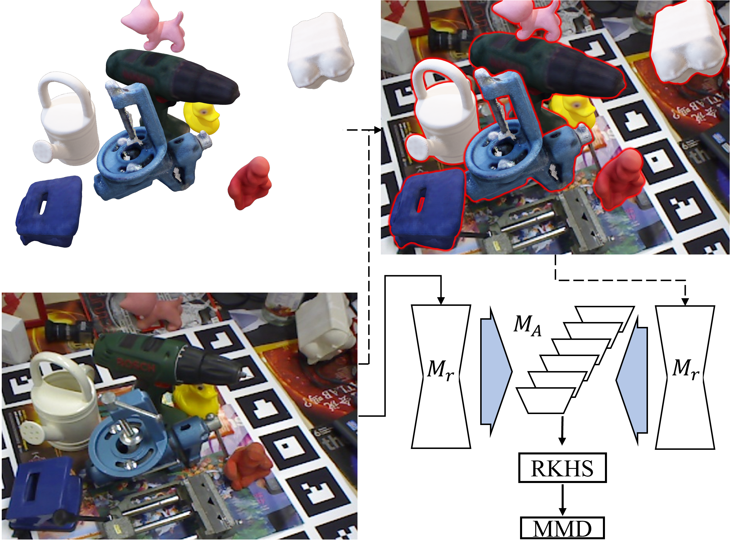
Figure 1: RKHSPose adapts the network pretrained on synthetic data (top left) to real test scenes (bottom left), by comparing network feature spaces with real image inputs (solid arrows), against those with syn/real image (top right) inputs (dashed arrows).

As with other machine learning (ML) tasks, 6DoF PE requires large annotated datasets. This requirement is particularly challenging for 6DoF PE, as the annotations comprise not only the identity of the objects in the scene, but also their 6DoF pose, which makes the data relatively expensive to annotate compared to related tasks such as classification, detection and segmentation. This is due to the fact that humans are not able to qualitatively or intuitively estimate 6DoF pose, which therefore requires additional instrumentation of the scene at data collection, and/or more sophisticated user interface tools [34, 87]. Consequently, synthetic 6Dof PE datasets [36, 43] have been introduced, either as an additional complement to a real dataset, or as a standalone purely synthetic dataset. Annotated synthetic datasets are of course trivially inexpensive to collect, simply because precise synthetic pose annotation in a simulated environment is fully automatic. A known challenge in using synthetic data, however, is that there typically exists a domain gap between the real and synthetic data, which makes results less accurate when using purely synthetic datasets. Expectations of the potential benefit of synthetic datasets has led to the exploration of a rich set of Domain Adaptation (DA) methods, which specifically aim to reduce the domain gap [6, 92, 64] using inexpensive synthetic data for a wide variety of tasks, recently including 6DoF PE [28, 46, 49].

Early methods [86, 42] ignored the simulation-to-real (sim2real) domain gap and, nevertheless improved performance by training on both synthetic and real data, effectively augmenting the real images with the synthetic. However, these methods still required real labels to be sufficiently accurate and robust for practical applications, partially due to the domain gap. As shown in Fig. 1, the rendered synthetic objects (left image) have a slightly different appearance than the real objects (right image). The details of the CAD models, both geometry and texture, are not precise, as can be seen for the can object (which lacks a mouth and shadows), the benchvise (which is missing a handle), and the holepuncher (which has coarse geometric resolution). Several recent methods [44, 73, 77, 9, 81] have started to address the sim2real gap for 6DoF PE by first training on labeled synthetic data and then fine-tuning on unlabeled real data. These methods, commonly known as self-supervised methods, reduce the domain gap by adding extra supervision using features extracted from real images without making use of real groundtruth (GT) labels. The majority of these methods are viewpoint/template matching-based, and the self-supervision commonly iteratively matches 2D masks or 3D point clouds.

While the above-mentioned self-supervison works have shown promise, there exist a wealth of DA techniques that can be brought to bear to improve performance further for this task. One such technique is Reproducing Kernel Hilbert Space (RKHS), which is a kernel method with a reproducing property in a Hilbert Space. RKHS was initially used to create decision boundaries for non-separable data [12, 62], and has been shown to be effective at reducing the domain gap for various tasks and applications [93, 67, 7]. The reproducing kernel guarantees that the domain gap can be statistically measured, allowing the real and synthetic data to be effectively comparable using specifically tailored metrics.

To address this sim2real domain gap in 6DoF PE, we propose RKHSPose, which is a keypoint-based method [86, 85] trained on a mixture of a large collection of labeled synthetic data, and a small handful of unlabeled real data. RKHSPose estimates the intermediate radial voting quantity, which has shown to be effective for estimating keypoints [86], by first training a modified FCN-Resnet-18 on purely synthetic data with synthetic GT poses. The radial quantity is a map of the distance from each image pixel to each keypoint. Next, real images are passed through the synthetically trained network, resulting in a set of pseudo-keypoints. The real images and their corresponding pseudo-keypoints are used to render a set of ‘synthetic-over-real’ (synth/real) images, by first estimating the pseudo-pose from the pseudo-keypoints, and then overlaying the synthetic object, rendered with the pseudo-pose, onto the real image. The network training then continues on the synth/real images, invoking an RKHS network module with a trainable linear product kernel, which minimizes the Maximum Mean Discrepancy (MMD) loss. At the front end, a proposed Keypoint Radial Vote Net (KRVNet) CNN learns to cast votes to estimate keypoints from the backend-generated radial maps. The final pose is then determined using ePnP [47] based on the estimated and corresponding object keypoints.

The main contributions of this work are:

• A novel learnable RKHS-based Adapter backend network to minimize the sim2real domain gap in 6DoF PE;

• A novel CNN-based frontend network KRVNet for keypoint radial voting;

• A self-supervised keypoint-based 6DoF PE method, RKHSPose, which is shown to have state-of-the-art (SOTA) performance, based on our experiments and several ablation studies.

2 Related Work

2.1 6DoF PE

Method CAD Syn Real Real Model Data Images Labels LatentFusion [61] ✗ ✓ ✗ ✗ FS6D [33] ✓ ✓ ✗ ✗ OSOP [69] ✓ ✓ ✗ ✗ AAE [73] ✓ ✓ ✗ ✗ MHP [56] ✓ ✓ ✗ ✗ Sock et al. [70] ✓ ✓ ✗ ✗ DSC [89] ✓ ✓ ✗ ✗ Xiao et al. [89] ✓ ✓ ✗ ✗ Sundermeyer [74] ✓ ✓ ✗ ✗ Kleeberger et al. [44] ✓ ✓ ✗ ✗ SO-Pose [18] ✓ ✓ ✓ ✓ Su et al. [71] ✓ ✓ ✓ ✗ Self6D [81] ✓ ✓ ✓ ✗ Self6D++ [82] ✓ ✓ ✓ ✗ Deng et al. [15] ✓ ✓ ✓ ✗ TexPose [9] ✓ ✓ ✓ ✗ SMOC-Net [77] ✓ ✓ ✓ ✗ DPODv2 [68] ✓ ✓ ✓ ✗ GDRNet [83] ✓ ✓ ✓ ✗ RKHSPose (Ours) ✓ ✓ ✓ ✗

Table 1: Existing self-supervised 6DoF PE methods. Some of the methods used CAD models, synthetic (syn) data with labels (GT pose), and real data without labels whereas others used only the labeled synthetic data. SO-Pose [18] used very few real labels to improve performance.

ML based 6DoF PE methods [87, 59, 63] all train a network to regress quantities, such as keypoints and camera viewpoints, as have been used in classical algorithms [34]. ML-based methods, which initially became popular in the general object detection field, have started to dominate the 6DoF PE literature due to their accuracy and efficiency.

There are two main categories of ML-based fully supervised methods: feature matching-based [87, 59, 72, 30, 29], and keypoint-based methods [63, 31, 32, 90]. Feature matching-based methods make use of the structures from general object detection networks most directly. The network encodes and matches features and estimates pose by either regressing elements of the pose (e.g. the transformation matrix [77], rotational angles and translational offsets [87] or 3D vertices [72]) directly, or by regressing some intermediate feature-matching representations, such as viewpoints or segments.

In contrast, keypoint-based methods encode features to estimate keypoints which are predefined within the reference frame of an object’s CAD model. These methods then use (modified) classical algorithms such as PnP [22, 47], Horn’s method [38], and ICP [3] to estimate the final pose. Unlike feature-matching methods, keypoint-based methods are typically more accurate due to the redundancies encountered through voting mechanisms [63, 86, 31] and by generating confidence hypotheses of keypoints [32, 90].

Recently, self-supervised 6DoF PE methods have been explored in order to reduce the reliance on labeled real data, which is expensive to acquire. As summarized in Table 1, these methods commonly use real images without GT labels. Some methods use pure synthetic data and CAD models only, with one exception [61] which trained the model using only synthetic data. The majority of these methods [33, 69, 74, 71, 81, 15, 82, 9, 77, 70] are inspired by the fully supervised feature-matching methods, except DPODv2 [68] and DSC [89], in which keypoint correspondences are rendered and matched.

A few methods [69, 15] fine-tuned the pose trivially by iteratively matching the template/viewpoint, whereas others [89, 44, 61, 33] augmented the training data by adding noise [89, 44], rendering textures [33, 68] and creating a latent space [61]. Some methods [73, 74, 56] also implemented Domain Adaptation (DA) techniques such as encoding a codebook [74], PCA [74] and symmetric Bingham distributions [56]. Most methods [69, 71, 81, 82, 70, 89] used rendering techniques to render and match a template. There are a few methods that combined 3D reconstruction techniques, such as Neural radiance fields (Nerf) [57] and Structure from Motion (SfM) [78]. TexPose [9] matched CAD models to segments generated by Nerf, and SMOC-Net [77] used SfM to create the 3D segment and matched with the CAD model.

2.2 Kernel Methods and Deep Learning

Although Deep Learning (DL) is the most common ML technique within the CV literature, kernel methods [12, 62, 66] have also been actively explored. Kernel methods are typically in a RKHS space [76] with reproducing properties so that non-linear problems can be solved by mapping input data into high dimensional spaces where those data can be linearly separated [23, 11]. Some well-known early kernel methods that have been applied to CV problems are Support Vector Machines [12] (SVMs) and Principle Component Analysis [62] (PCA). One recent method [66] linked energy distance and MMD in RKHS, and showed the effectiveness of kernels in statistical hypothesis testing.

More recent studies compare kernel methods with DL networks. RKHS is found to be performing better on classification tasks than one single block of a Convolutional Neural Network (CNN) comprising convolution, pooling and downsampling (linear) layers [41]. RKHS can also help with the generalization of CNN by meta-regularization on image registration problems[1]. Similarly, norms defined in RKHS help with the regularization of CNN [5, 4]. Further, discriminant information in label distributions in unsupervised DA is addressed and RKHS-based Conditional Kernel Bures metric is proposed [52] . Lastly, the connection between Neural Tangent Kernel and MMD is established, and an efficient MMD for two-sample tests is developed [10].

Inspired by the previous work, RKHSPose applies concepts of kernel learning to keypoint-based 6DoF PE, to provide an effective means to self-supervise a synthetically trained network on unlabelled real data.

3 Method

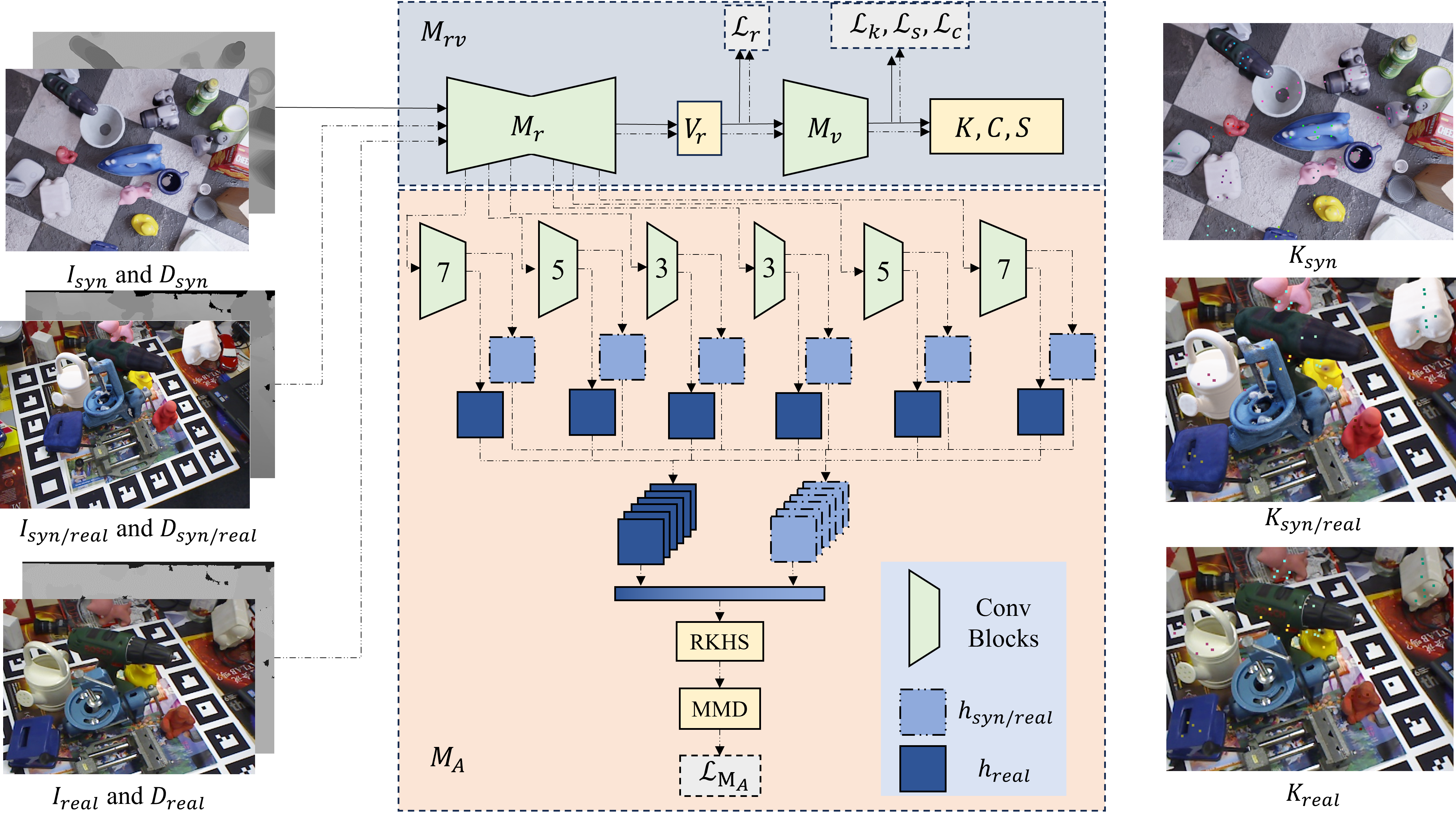
Figure 2: RKHSPose architecture. RKHPose is first trained on synthetic labeled data (solid arrows), and then finetuned on alternating syn/real and (unlabelled) real images (dashed arrows). $M_{A}$ is measured by MMD in RKHS by densely mapping the intermediate features of $M_{r}$ into high dimensional spaces with conv blocks. The distance is treated as $\mathcal{L}_{M_{A}}$ and back-propagated through $M_{A}$ and $M_{r}$.

3.1 Network Overview

As shown in Fig. 2, RKHSPose is made up of two networks, one main network $M_{rv}$ for keypoint regression and classification, and one Adapter network $M_{A}$ to minimize the synthetic-real domain gap by densely comparing the feature maps of every convolution block of $M_{rv}$ trained on both synthetic and real images.

The input of $M_{rv}$ with shape $W\!\times\!H\!\times\!4$, is the concatenation of an RGB image $I$ and its corresponding depth map $D$. This input can be synthetically generated with an arbitrary background ($I_{syn}$ and $D_{syn}$), a synthetic mask overlayed on a real background ($I_{syn/real}$ and $D_{syn/real}$), or real ($I_{real}$ and $D_{real}$) images. The outputs are $n$ projected 2D keypoints $K$, along with corresponding classification labels $C$ and visibility scores $S$.

The main network $M_{rv}$ comprises two sub-networks, regression network $M_{r}$ and voting network $M_{v}$. Inspired by recent voting techniques [63, 31, 86, 85, 94], $M_{r}$ estimates an intermediate voting quantity, which is a radial distance map $V_{r}$ [86], by using a modified Fully Connected ResNet 18 (FCN-ResNet-18). The radial voting map $V_{r}$ , with shape $W\!\times\!H$, stores the Euclidean distance from each object point to each keypoint in the 3D camera world reference frame. The voting network $M_{v}$ (described in Sec. 3.3) then takes $V_{r}$ as input, accumulates votes, detects the peak, and estimates the final keypoints $K$, classification labels $C$ and confidence scores $S$.

The Adapter model $M_{A}$ consists of a series of CNNs which encode pairs of feature maps from $M_{rv}$, and are trained on both synthetic overlayed and pure real data. $M_{A}$ encodes feature map pairs $(f_{syn/real},f_{real})$ into corresponding high-dimensional feature maps $(h_{syn/real},h_{real})$. The input data, $(I_{syn/real},I_{real})$ and $(D_{syn/real},D_{real})$, are also treated as $(f_{syn/real},f_{real})$ during the learning of $M_{A}$. Each of these networks creates a high-dimensional latent space, essentially the Reproducing Kernel Hilbert Space (RKHS) [2] and contributes to the learning of both $M_{rv}$ and $M_{A}$ by calculating the MMD [27].

The loss function $\mathcal{L}$ is made up of five elements: Radial regression loss $\mathcal{L}_{r}$ for $V_{r}$; Keypoint projection loss $\mathcal{L}_{k}$ for $K$; Classification loss $\mathcal{L}_{c}$ for $C$; Confidence loss $\mathcal{L}_{s}$ for $S$, and finally; Adapter loss $\mathcal{L}_{M_{A}}$ for the comparison of intermediate feature maps. The regression losses $\mathcal{L}_{r}$, $\mathcal{L}_{k}$, and $\mathcal{L}_{s}$ all use the smooth L1 metric, whereas classification loss $\mathcal{L}_{c}$ uses the cross-entropy metric. RKHSPose losses can then be denoted as:

$$\mathcal{L}_{r} = smooth_{\mathcal{L}_{1}}(V_{r},\widehat{V_{r}})$$ (1)

$$\mathcal{L}_{k} = smooth_{\mathcal{L}_{1}}(K,\widehat{K})$$ (2)

$$\mathcal{L}_{c} = H(p(C),\widehat{p(C)})$$ (3)

$$\mathcal{L}_{s} = smooth_{\mathcal{L}_{1}}(S,\widehat{S})$$ (4)

$$\mathcal{L}_{M_{A}} = MMD(\widehat{f_{syn/real}},\widehat{f_{real}})$$ (5)

$$\mathcal{L}=\lambda_{r}\mathcal{L}_{r}+\lambda_{k}\mathcal{L}_{k}+\lambda_{c}\mathcal{L}_{c}+\lambda_{s}\mathcal{L}_{s}+\lambda_{D}\mathcal{L}_{M_{A}}$$ (6)

where $\lambda_{r}$, $\lambda_{k}$, $\lambda_{c}$, $\lambda_{s}$, and $\lambda_{D}$ are weights for adjustment during training, and all non-hatted quantities are GT values.

At inference, $M_{rv}$ takes the $I_{real}$ and $D_{real}$ as input, and outputs $K$, $C$ and $S$. The keypoints $K$ are ranked and grouped by $S$ and $C$, and are then forwarded into the ePnP [47] algorithm which estimates a 6DoF pose value.

3.2 Convolutional RKHS Adapter

Reproducing Kernel Hilbert Space $\mathcal{H}$ is a commonly used vector space for Domain Adaptation [60, 79]. Hilbert Space is a complete metric space (in which every Cauchy sequence of points has a limit within the metric) represented by the inner product of vectors. For a non-empty set of data $\mathcal{X}$, a function $K_{X}\!:\!\mathcal{X}\!\times\!\mathcal{X}\!\rightarrow\!\mathcal{R}$ is a reproducing kernel if:

$$\begin{cases}&k(\cdot,x)\in\mathcal{H}\;\;\;\forall\;\;\;x\in\mathcal{X}\\ &\left\langle f(\cdot),k(\cdot,x)\right\rangle=f(x)\;\;\;\forall\;\;\;x\in\mathcal{X},f\in\mathcal{H}\end{cases}$$ (7)

where $\left\langle a,b\right\rangle$ denotes the inner product of two vectors $a$ and $b$, $k(\cdot,x)=K_{\mathcal{X}}$ for each $x\!\in\!\mathcal{X}$, and $f$ is a function in $\mathcal{H}$. The second equation in Eq. 7 is an expression of the reproducing property of $\mathcal{H}$.

In order to utilize $\mathcal{H}$ for DA, we expand the kernel definition to two sets of data $\mathcal{X}$ and $\mathcal{Y}$. The reproducing kernel can then be defined as:

$$K(\mathcal{X},\mathcal{Y})=\left\langle K_{\mathcal{X}},K_{\mathcal{Y}}\right\rangle_{H}$$ (8)

Here, $K_{\mathcal{X}}$ and $K_{\mathcal{Y}}$ are themselves inner product kernels that map $\mathcal{X}$ and $\mathcal{Y}$ respectively into their own Hilbert spaces, and $K(\mathcal{X},\mathcal{Y})$ is the joint Hilbert space kernel of $\mathcal{X}$ and $\mathcal{Y}$.

Note that $K(\mathcal{X},\mathcal{Y})$ is not the kernel commonly defined for CNNs. Rather, it is the similarity function defined in kernel methods, such as is used by SVM techniques to calculate similarity measurements. Some recent methods [58, 55, 54, 8] named it a Convolutional Kernel Network (CKN) in order to distinguish it from CNNs.

Various kernels of CKN, such as the Gaussian Kernel [55], the RBF Kernel [54] and the Inner Product Kernel [58], have been shown to be comparable to shallow CNNs for various tasks, especially for Domain Adaption. The most intuitive inner product kernel is mathematically similar to a Fully Connected (FC) Layer, where trainable weights are multiplied by the input feature map. To allow the application of RKHS methods into our CNN based Adapter network $M_{A}$, trainable weights are added to $K(\mathcal{X},\mathcal{Y})$ [50]. The trainable Kernel $K_{w}(\mathcal{X},\mathcal{Y})$ can then be denoted as:

$$K_{w}(\mathcal{X},\mathcal{Y})=\left\langle\left\langle\mathcal{X},W_{\mathcal{X}}\right\rangle,\left\langle\mathcal{Y},W_{\mathcal{Y}}\right\rangle\right\rangle_{H}$$ (9)

where $W_{\mathcal{X}}$ and $W_{\mathcal{Y}}$ are trainable weights. By adding $W_{\mathcal{X}}$ and $W_{\mathcal{Y}}$ , $K_{w}(\mathcal{X},\mathcal{Y})$ still satisfies RKHS constraints.

The synthetic-real domain gap of feature maps $f$ being trained in $M_{rv}$ (with few real images and no real GT labels) are hard to measure using trivial distance metrics. In contrast, RKHS can be a more accurate and robust space for comparison, since it is known to be capable of handling high-dimensional data with a low number of samples [24, 58]. To compare $(f_{syn/real},f_{real})$ in RKHS, a series of CNN layers encodes $(f_{syn/real},f_{real})$ into higher-dimensional features $(h_{syn/real},h_{real})$, followed by the trainable $K_{w}(\mathcal{X},\mathcal{Y})$. Once mapped into RKHS, $h_{syn/real}\!=\!\{sr_{i}\}_{i=1}^{m}$ and $h_{real}\!=\!\{r_{i}\}_{i=1}^{m}$ can then be measured by Maximum Mean Discrepancy (MMD), a common DA measurement [27, 50], which is the square distance between the kernel embedding [26]:

$$MMD( h_{syn/real},h_{real})=\hskip 85.35826pt$$ (10)

$$\left[\frac{1}{m^{2}}\right. \left(\left(\sum_{i=1}^{m}\sum_{j=1}^{m}{k_{w}(sr_{i},sr_{j})}\right.\right.-\left.\sum_{i=1}^{m}{k_{w}(sr_{i},sr_{i})}\right)$$

$$-\left(\sum_{i=1}^{m}\sum_{j=1}^{m}{k_{w}(sr_{i},r_{j})}\right.-\left.\sum_{i=1}^{m}{k_{w}(sr_{i},r_{i})}\right)$$

$$+\left(\sum_{i=1}^{m}\sum_{j=1}^{m}{k_{w}(r_{i},r_{j})}\right.-\left.\left.\left.\sum_{i=1}^{m}{k_{w}(r_{i},r_{i})}\right)\right)\right]^{0.5}$$

In summary, the Adapter $M_{A}$, shown in Fig. 2, measures MMD for each $(h_{syn/real},h_{real})$ in RKHS by increasing the $f_{syn/real}$ and $f_{real}$ dimension using a CNN and thereby constructing a learnable kernel $K_{w}$. The output are the feature maps $h_{syn/real}$ and $h_{real}$ which are supervised by loss $\mathcal{L}_{M_{A}}$, during training of the real data epochs. Based on the experiments in Sec. 5.1, our trainable inner product kernel is shown to be more accurate for our task than other known kernels [55, 54, 58] used in such kernel methods.

3.3 Keypoint Radial Vote Net

Keypoint Radial Vote Net (KRVNet) votes for keypoints using a CNN network architecture, taking the radial voting quantity resulting from $M_{v}$ as input. VoteNet [65] previously used a CNN approach to vote for object centers, whereas other keypoint-based techniques have implemented GPU-based parallel RANSAC [31, 63] methods for offset and vector quantities. The radial quantity is known to be more accurate but less efficient than the vector or offset quantities, and has been previously implemented with a CPU-based parallel accumulator space method [86, 85].

Given its superior accuracy, KRVNet $M_{v}$ implements radial voting using a CNN to improve efficiency. The voting is parallelized on a GPU, and jointly estimates confidence scores alongside the radial votes themselves, thereby improving robustness. Given a 2D radial map $\widehat{V_{r}}$ estimated by $M_{r}$ and supervised by GT radial maps $V_{r}$, the task is to accumulate votes, find the peak, and estimate the keypoint location. The $V_{r}$ foreground pixels (which lie on the target object) store the Euclidean distance from these pixels to each of the keypoints, with background (non-object) pixels set to value $-1$.

The estimated radial map $\widehat{V_{r}}$ is indeed an inverse heat map of the candidate keypoints’ locations , distributed in a radial pattern centered at the keypoints. To forward $\widehat{V_{r}}$ into a CNN voting module, it is inversely normalized so that it becomes a heat map. Suppose that $v^{max}_{r}$ and $v^{min}_{r}$ are the maximum and minimum global radial distances of all objects in a dataset, which can be calculated by iterating through all GT radial maps, or alternately generated from the object CAD models. An inverse radial map $\widehat{V^{-1}_{r}}$ can then be denoted as:

$$\widehat{V^{-1}_{r}}=(v^{max}_{r}\!-\!\widehat{V_{r}})/(v^{max}_{r}\!-\!v^{min}_{r})$$ (11)

Thus, $M_{v}$ takes $\widehat{V^{-1}_{r}}$ as the input and generates the accumulated vote map by a series of convolution, ReLu, and batch normalization layers. The complete network architecture is provided in the Supplementary material. The background pixels are filtered out by a ReLu layer, and only foreground pixels contribute to voting. The accumulated vote map is then max-pooled (peak extraction) and reshaped using a fully connected layer into a $n\!\times\!4$ output. The output represents $n$ keypoints and comprises $n\!\times\!2$ projected 2D keypoint $K$, $n$ classification labels $C$, and $n$ confidence scores $S$. The labels $C$ indicate which object the corresponding keypoint belongs to, and $S$ ranks the confidence level of keypoints before being forwarded into ePnP [47] for pose estimation. KRVNet $M_{v}$ is supervised by $\mathcal{L}_{k}$, $\mathcal{L}_{c}$, and $\mathcal{L}_{s}$, and is trained end-to-end with $M_{r}$.

4 Experiments

4.1 Datasets and Evaluation Metrics

RKHSPose uses BOP Procedural Blender [17] (PBR) synthetic images [36, 37, 75, 16] for the synthetic training phase. The images are generated by dropping synthetic objects (CAD models) onto a plane in a simulated environment using PyBullet [13], and then rendering them with synthetic textures. All objects in the synthetic images are thus directly labeled with precise GT poses.

We evaluated RKHSPose for the six BOP [37, 75] core datasets (LM (LMO) [34], YCB-V (YCB) [87], TLESS [35], TUDL [36], ITODO [20], and HB [40]) all except IC-BIN [19], which does not include any real training and validation images and is therefore not applicable. ITODO and HB have no real images in the training set, and so instead we used the real images in their validation sets, which were disjoint from their test sets.

Our main results are evaluated with the ADD(S) [34] metric for the LM and LMO dataset, and the ADD(S) AUC [87] metric for the YCB dataset. These are the standard metrics commonly used to compare self-supervised 6DoF PE methods. ADD(S) is based on the mean distance (minimum distance for symmetry) between the object surfaces for GT and estimated poses, whereas ADD(S) AUC plots a curve formed by ADD(S) for various object diameter thresholds. We use the BOP average recall ($AR$) metrics for our ablation studies. The $AR$ metric, based on the original ADD(S) [34], evaluates three aspects, including Visible Surface Discrepancy ($AR_{VSD}$), Maximum Symmetry-Aware Surface Distance ($AR_{MSSD}$), and Maximum Symmetry-Aware Projection Distance ($AR_{MSPD}$).

4.2 Implementation Details

RKHSPose is trained on a server with an Intel Xeon 5218 CPU and 2 RTX6000 GPUs with a batch size of 32. The Adam optimizer is used for the training of $M_{rv}$, on both synthetic and real data, and $M_{A}$ is optimized by SGD. Both of the optimizers have an initial learning rate of $lr\!=\!1e-3$ and weight decay for $80$ and $20$ epochs respectively.

The input of the network is normalized before training, as follows. The images $I$ are normalized and standardized using ImageNet [14] specifications. The depth maps $D$ are normalized by their local minima and maxima, to lie within a range of 0 to 1. The radial distances in radial map $V_{r}$ and 2D projected keypoints are both normalized by the width and height of $I$. A single set of keypoints is chosen by KeyGNet [84] for the set of all objects in each dataset. One extra class is added to $C$ in order to filter out the redundant background points in $K$.

$M_{rv}$ is first trained for $120$ epochs on synthetic data, during which $M_{A}$ remains frozen. Following this, training proceeds for an additional $80$ epochs which alternate between real and synthetic data. When training on real data, both $M_{A}$ and $M_{rv}$ weights are learned, whereas $M_{A}$ is frozen for the alternating synthetic data training.

During real data epochs, $M_{rv}$ initially estimates pseudo-keypoints for each real image. These pseudo-keypoints are then forwarded into ePnP for pseudo-pose estimation. Each estimated pseudo-pose is then augmented into a set of poses $P_{aug}$, by applying arbitrary rotational and translational perturbations. Rotational perturbation $\Delta_{R}$ and translational perturbation $\Delta_{T}$ have respective ranges of $[-\frac{\pi}{18},\frac{\pi}{18}]$ radians and $[-0.1,0.1]$ along three axes within the normalized model frame, which is defined using the largest object in the dataset. The set of hybrid synthetic/real images are rendered by overlaying onto the real image the CAD model of each object using each augmented pose value in $P_{aug}$. The cardinality of $P_{aug}$ is set to be one less than the batch size, and the adapter $M_{A}$ is trained on a mini-batch of the hybrid images resulting from $P_{aug}$, plus the image resulting from the original estimated pseudo-pose.

Initially $M_{A}$ is frozen, and for the first $80$ epochs, the loss is set to emphasize the classification and the visibility score regression, i.e. $\lambda_{c}\!=\!\lambda_{s}\!=\!0.6$ and $\lambda_{r}\!=\!\lambda_{k}\!=\!0.4$. Following this, up to epoch $200$, the scales of losses are then exchanged to fine-tune the localization of the keypoints, i.e. $\lambda_{c}\!=\!\lambda_{s}\!=\!0.4$ and $\lambda_{r}\!=\!\lambda_{k}\!=\!0.6$. After epoch $120$, $M_{A}$ is unfrozen each alternating epoch, and $\lambda_{D}$ is set to 1 during the $M_{A}$ training epochs. This training strategy, shown in Fig. 2, minimizes the synthetic-to-real gap without any real image GT labels, and using very few real images.

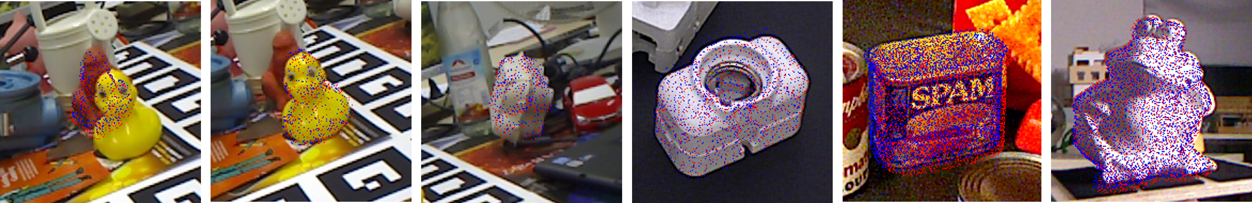
Figure 3: Qualitative overlay results on selected datasets. Red dots are projected GT poses and blue dots are projected estimated poses. The estimated overlay is better aligned visually for some objects (ape in LMO, potted meat can in YCB, and frog in TUDL), possibly due to the accurate synthetic labels.

4.3 Results

Dataset Methods Real LM LMO YCB data ADD(S) ADD-S ​img​ ​lbl​ ADD(S) AUC AUC AAE [73] ✗ ✗ 31.4 - - - MHP [56] ✗ ✗ 38.8 - - - GDR^∗∗ [83] ✗ ✗ 77.4 52.9 - - Sock et al. [70] ✓ ✗ 60.6 22.8 - - DSC [91] ✓ ✗ 58.6 24.8 - - Self6D [81] ✓ ✗ 58.9 32.1 - - SMOC-Net [77] ✓ ✗ 91.3 63.3 - - Self6D++ [82] ✓ ✗ 88.5 64.7 80.0 91.4 TexPose [9] ✓ ✗ 91.7 66.7 - - Ours ✓ ✗ 95.8 68.6 82.8 92.4 Ours+ICP ✓ ✗ 95.9 68.7 83.0 92.6

Table 2: Accuracy results on LM, LMO and YCB datasets: accuracy of RKHSPose for LM and LMO is evaluated with ADD(S), and for YCB is evaluated with ADD(S) AUC. Under ‘Real Data’, ‘img’ stands for images and ‘lbl’ stands for labels. All syn/real methods use real images without real (GT) labels. Methods annotated with ^∗∗ are the TexPose [9] re-implementation.

Methods real Dataset lbl LM LMO TLESS TUDL ITODD HB YCB MegaPose^∗ [45] ✓ - 70.4 71.8 91.6 59.2 87.2 85.5 SurfEmb^∗ [30] ✓ - 76.0 82.8 85.4 65.9 86.6 79.9 RCVPose3D [85] ✓ - 72.9 70.8 96.6 73.3 86.3 84.3 PFA^∗ [39] ✓ - 79.2 84.9 96.3 70.6 86.7 89.9 ZebraPose [72] ✓ - 78.0 86.2 95.6 65.4 92.1 89.9 GDRNPP [83, 51] ✓ - 77.5 87.4 96.6 72.2 92.6 92.1 Ours ✗ 95.7 68.2 85.5 96.2 68.6 92.2 83.6 Ours+ICP ✗ 95.8 68.4 85.6 96.2 68.7 92.3 83.8

Table 3: BOP AR results compared to fully supervised methods with real GT labels on BOP leaderboard: RKHSPose results on TLESS ($-1.8$), TUDL ($-0.4$), ITODD ($-4.6$) and HB ($-0.3$) compares to SOTA methods with full supervision of real GT labels. RKHSPose performs second best on HB. Methods annotated with ^∗ use the detection results by other detection methods.

The results are summarized in Tables 2 and 3. To the best of our knowledge, RKHSPose outperforms all existing self-supverised 6DoF PE methods. Specifically, on LM and LMO, our ADD(S) is $+4.2\%$ and $+2\%$ better than the second best method TexPose [9]. Although very few methods evaluate on YCB, we nevertheless compared our performance to self6D++ [82] and made $3\%$ improvements after ICP on ADD(S) AUC. Last but not least, our performance evaluated on the other four BOP core datasets is comparable to several SOTA methods from the BOP leaderboard, which are fully supervised with real labels (Table 3). Some test scenes of RKHSPose are shown in Fig. 3.

RKHSPose runs at 34 fps on an Intel i7 2.5GHz CPU and an RTX 3090 GPU with 24G VRAM. Specifically, it takes $8.7ms$ for loading data, $4.5ms$ for forward inference through $M_{rv}$, and $16.2ms$ for ePnP.

5 Ablation Studies

5.1 Dense Vs. Sparse Adapter

Adapter $AR_{VSD}$ $AR_{MSSD}$ $AR_{MSPD}$ $AR$ $M^{s}_{A}$ 78.1 77.8 77.8 77.9 $M_{A}$ 84.9 84.1 84.3 84.4

Table 4: Average $AR$ of different Adapters on LM and six BOP core datasets.

The Adapter $M_{A}$ densely matches the intermediate feature maps, whereas the majority of other methods [77, 15, 81] only compare the final output. In order to show the necessity of dense comparison, we conduct an experiment with different variations of $M_{A}$. A sparse matching $M^{s}_{A}$, is trained on synthetic and real data comparing only a single feature map, which is the intermediate radial map. $M^{s}_{A}$ has the exact same overall learning capacity (number of parameters) as the dense matching $M_{A}$ described in Sec. 3.3.

The results are shown in Table 4. $M_{A}$ surpassed $M^{s}_{A}$ on all six datasets tested. Specifically, on ITODD, $M_{A}$ is $12.1\%$ more accurate than $M^{s}_{A}$. This experiment shows the effectiveness of our densely matched $M_{A}$.

5.2 Adapter Kernels and Metrics

Kernels $w$ $AR_{VSD}$ $AR_{MSSD}$ $AR_{MSPD}$ $AR$ Linear ✗ 71.6 70.8 70.6 71.0 ✓ 84.9 84.1 84.3 84.4 RBF ✗ 73.4 72.9 73.2 73.2 ✓ 82.5 81.3 81.5 81.6

Table 5: Average $AR$ of different RKHS kernels on LM and five BOP core datasets.

Metrics $AR_{VSD}$ $AR_{MSSD}$ $AR_{MSPD}$ $AR$ MMD 84.9 84.1 84.3 84.4 KL Div 78.0 77.8 78.0 77.9 Wass Distance 80.9 80.6 80.9 80.8

Table 6: Average $AR$ of different metrics on LM and five BOP core datasets.

We use linear (dot product) kernel and MMD in RKHS for domain gap measurements. There are various other kernels and similarity measurements that can be implemented in RKHS as described in Sec. 3.2. First, we add trainable weights to the RBF kernel in a similar manner of $K_{w}$ defined in Eq. 9. The trainable RBF kernel on two sets of data $X$ and $Y$ can be denoted as:

$$K_{rbf}(X,Y)=exp(-w\left\|X-Y\right\|^{2})$$ (12)

where $w$ is the trainable weights, which replaces the original adjustable parameter in the classical RBF kernel.

We also experiment with the classical RKHS kernel functions, including the inner product kernel and the RBF kernel [80], for comparison. Further, we experiment on other commonly used distance measures, including Kullback-Leibler Divergence (KL Div, i.e. relative-entropy) and Wasserstein (Wass) Distance.

In Table 5, the RBF kernel performs very similarly to the linear product kernel with a slight performance dip. In Table 6, MMD minimizes the domain gap better than the Wass Distance, followed by the KL Div metric, leading to a better overall performance on $AR$. Based on these results, we therefore We use the linear product kernel, and chose MMD as the main loss metric in our final structure.

5.3 Syn/Real Synchronized Training

Training Type $AR_{VSD}$ $AR_{MSSD}$ $AR_{MSPD}$ $AR$ Mixed 84.9 84.1 84.3 84.4 Sequantial 82.3 81.7 81.7 81.9

Table 7: The average $AR$ of different Training Strategies on LM and five BOP core datasets.

When training RKHSPose, real epochs are alternated with synthetic epochs. In contrast, some other methods [9, 81, 82, 77] separate the synthetic/real training. We conducted an experiment to compare these two different training strategies, the results of which are shown in Table 7. The alternating training performs slightly better ($+2.5\%$ on average) than the sequential training, possibly due to the early access to real scenes thereby avoiding local minima.

5.4 Number of Real Images and Real Labels

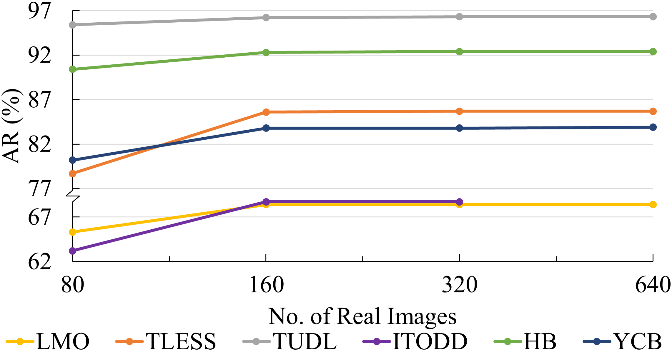
Figure 4: Impact of No. of real images without GT labels used during training. All datasets are evaluated by the BOP AR metric. There are only 357 real training images available in ITODD, and we only conduct experiments from 80 to 320 real images. For those datasets in which there is only one object per real image, we use $No.\_of\_Objects\!\times\!No.\_of\_Images$ so that it is a fair comparison against other datasets.

The objective of RKHSPose is to reduce real data usage and train without any real GT labels. To show the effectiveness of the approach, we conducted an experiment by training on different numbers of real images, the results of which are shown in Fig. 4. We used 640 real images in all cases, except for that of ITODD which contains only 357 real images. The $AR$ of all datasets saturates at 160 images except YCB. The improvement of YCB is also only $0.1\%$ and saturates after 320 real images. We nevertheless conservatively use $320$ real images for our main results.

6 Conclusion

To sum up, we propose a novel self-supervised keypoint radial voting-based 6DoF PE method using RGB-D data called RKHSPose. RKHSPose fine-tunes poses pre-trained on synthetic data by densely matching features with a learnable kernel in RKHS, using real data albeit without any real GT poses. By applying this DA technique in feature space, RKHSPose achieved SOTA performance on six BOP core datasets, surpassing the performance of all other self-supervised methods. Notably, the RKHSPose performance closely approaches that of several fully-supervised methods, which indicates the strength of the approach at reducing the sim2real domain gap for this problem.

In future work, we will explore the extension of these methods to the problem of novel object 6DoF PE, in which initial CAD models of the target objects are unavailable during training.

Limitations: A limitation of RKHSPose is that it relies on the accuracy of estimated pseudo-keypoints, which at the beginning of the training process, are initially generated purely from processing synthetic data, and therefore depend upon the similarity between the domains of the real and synthetic images. If this domain gap is too large, then the initial pseudo-keypoints could be inaccurate, which could degrade performance.

Supplementary Material

7 Overview

We document here some addition implementation details and results. The detailed structures of Keypoint Radial Vote Net (KRVNet) $M_{v}$ and Convolutional RKHS Adapter $M_{A}$ are shown in Figs. 5 and 6. Fig. 7 shows the visualized radial pattern of the dragon object in TUDL, which inspired us to use a CNN (KRVNet $M_{v}$) to simulate the voting process. The $AR_{VSD}$, $AR_{MSSD}$, $AR_{MSPD}$, and $AR$ results of all datasets we used for all ablation studies are listed in Tables 8, 9, 10, and 11. Last but not least, detailed ADD(S) results for each category of object on LM and LMO are listed in Tables 12 and 13, and ADD-S AUC results on YCB are shown in Table 14.

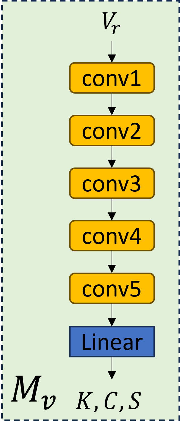
Figure 5: KRVNet $M_{v}$ detailed structure. Each conv block comprises convolution, batch normalization, and ReLu layers. The final linear layer reshapes the feature map into the output $K,C,S$.

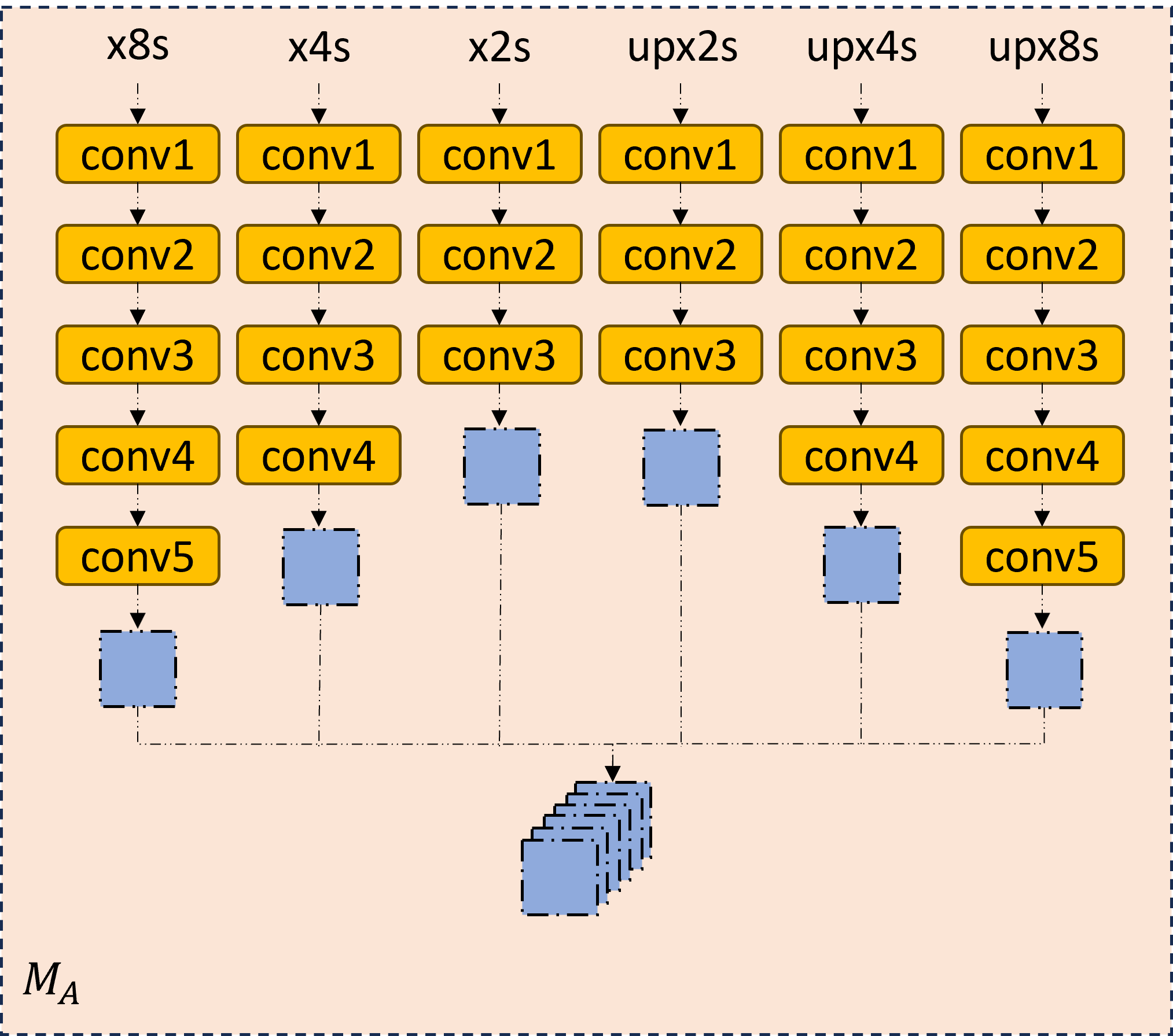
Figure 6: Covolutional RKHS Adapter $M_{A}$ detailed structure. Each conv block comprises convolution, batch normalization, and ReLu layers. Inputs of $M_{A}$, i.e. x8s, x4s, x2s, upx2s, upx4s, and upx8s are feature maps extracted from each stage of $M_{r}$. Outputs of each column of conv blocks are concatenated and mapped into RKHS by a linear layer.

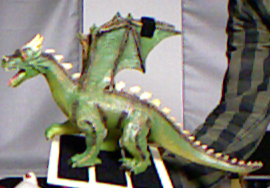
(a) RGB image

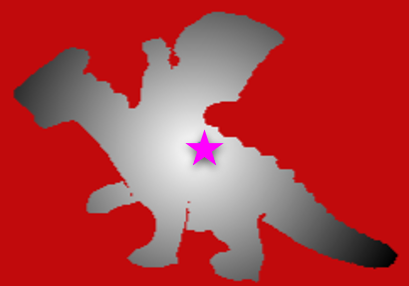
(b) center keypoint $\widehat{V^{-1}_{r}}$

(c) left keypoint $\widehat{V^{-1}_{r}}$

(d) right keypoint $\widehat{V^{-1}_{r}}$

Figure 7: TUDL [36] dataset dragon object (a) RGB image and (b)-(d) inverse radial maps $\widehat{V^{-1}_{r}}$. Keypoints (pink stars) are located at the (b) center, (c) left, and (d) right.

Adapter Dataset $AR_{VSD}$ $AR_{MSSD}$ $AR_{MSPD}$ $AR$ $M_{A}$ LM 96.0 95.7 95.7 95.8 LMO 68.7 68.2 68.2 68.4 TLESS 85.9 85.1 85.8 85.6 TUDL 97.6 96.4 95.4 96.2 ITODD 69.2 68.5 68.4 68.7 HB 92.7 91.6 92.5 92.3 YCB 83.9 83.4 84 83.8 2-62.5 average 84.9 84.1 84.3 84.4 $M^{s}_{A}$ LM 93.4 92.7 92.6 92.9 LMO 59.7 59.3 59.2 59.4 TLESS 78.8 78.7 78.8 78.8 TUDL 95.6 95.3 95.5 95.5 ITODD 56.7 56.7 56.5 56.6 HB 85.7 85.3 85.6 85.5 YCB 76.5 76.4 76.6 76.5 2-62.5 average 78.1 77.8 77.8 77.9

Table 8: The impact of sparse ($M^{s}_{A}$) and dense ($M_{A}$) Adapters defined in Sec. 5.1 in the main paper on LM and five BOP core datasets.

Kernels $w$ Dataset $AR_{VSD}$ $AR_{MSSD}$ $AR_{MSPD}$ $AR$ Linear ✗ LM 85.4 84.2 84.4 84.7 LMO 56.9 56.3 55.4 56.2 TLESS 74.3 73.8 74.2 74.1 TUDL 88.2 87.3 84.3 86.6 ITODD 45.2 44.7 45.3 45.1 HB 79.3 78.6 79.2 79.0 YCB 72.2 70.5 71.3 71.3 3-72.5 average 71.6 70.8 70.6 71.0 1-73 RBF ✗ LM 85.3 84.1 84.3 84.6 LMO 57.1 56.3 55.2 56.2 TLESS 73.7 73.1 73.6 73.5 TUDL 90.3 89.7 89.9 90.0 ITODD 52.7 51.9 52.5 52.4 HB 80.2 79.6 79.3 79.7 YCB 72.6 71.8 71.5 72.0 3-72.5 average 73.4 72.9 73.2 73.2 Linear ✓ LM 96.0 95.7 95.7 95.8 LMO 68.7 68.2 68.2 68.4 TLESS 85.9 85.1 85.8 85.6 TUDL 97.6 96.4 95.4 96.2 ITODD 69.2 68.5 68.4 68.7 HB 92.7 91.6 92.5 92.3 YCB 83.9 83.4 84 83.8 3-72.5 average 84.9 84.1 84.3 84.4 1-73 RBF ✓ LM 94.7 94.5 94.4 94.5 LMO 57.1 56.3 55.2 56.2 TLESS 83.7 82.9 83.3 83.3 TUDL 97.4 95.8 94.9 95.1 ITODD 66.7 63.6 64.2 64.7 HB 85.6 83.9 84.8 84.8 YCB 82.8 82.6 82.8 82.7 3-72.5 average 82.5 81.3 81.5 81.6

Table 9: The impact of different RKHS kernels defined in Sec. 5.2 in the main paper on LM and five BOP core datasets.

Metrics Dataset $AR_{VSD}$ $AR_{MSSD}$ $AR_{MSPD}$ $AR$ MMD LM 96.0 95.7 95.7 95.8 LMO 68.7 68.2 68.2 68.4 TLESS 85.9 85.1 85.8 85.6 TUDL 97.6 96.4 95.4 96.2 ITODD 69.2 68.5 68.4 68.7 HB 92.7 91.6 92.5 92.3 YCB 83.9 83.4 84 83.8 2-62.5 average 84.9 84.1 84.3 84.4 KL LM 90.2 90.3 90.5 90.3 Div LMO 63.4 62.2 63.6 63.1 TLESS 79.8 79.7 80.2 79.9 TUDL 93.4 93.2 92.9 93.2 ITODD 62.1 62.2 62.1 62.1 HB 84.6 84.3 84.7 84.5 YCB 72.6 72.5 72.3 72.4 2-62.5 average 78.0 77.8 78.0 77.9 Wass LM 92.3 91.7 92.2 92.1 Distance LMO 64.7 64.2 64.7 64.5 TLESS 82.3 82.2 81.9 82.1 TUDL 95.7 95.6 95.5 95.6 ITODD 65.7 64.9 65.6 65.4 HB 89.3 89.1 89.5 89.3 YCB 76.5 76.3 76.6 76.4 2-62.5 average 80.9 80.6 80.9 80.8

Table 10: The impact of different metrics defined in Sec. 5.2 in the main paper for $M_{A}$ on LM and five BOP core datasets.

Training Type Dataset $AR_{VSD}$ $AR_{MSSD}$ $AR_{MSPD}$ $AR$ Mixed LM 96.0 95.7 95.7 95.8 LMO 68.7 68.2 68.2 68.4 TLESS 85.9 85.1 85.8 85.6 TUDL 97.6 96.4 95.4 96.2 ITODD 69.2 68.5 68.4 68.7 HB 92.7 91.6 92.5 92.3 YCB 83.9 83.4 84 83.8 2-62.5 average 84.9 84.1 84.3 84.4 Sequantial LM 95.4 95.2 95.3 95.3 LMO 65.3 65.2 65.2 65.2 TLESS 85.7 85.3 85.6 85.5 TUDL 97.6 96.4 95.4 96.2 ITODD 63.4 62.2 62.3 62.6 HB 88.6 88.4 88.3 88.4 YCB 79.8 79.5 80.0 79.8 2-62.5 average 82.3 81.7 81.7 81.9

Table 11: The impact of different training strategies described in Sec. 5.3 in the main paper on LM and five BOP core datasets.

		Object
			bench-								hole-
Mode	Method	ape	vise	camera	can	cat	driller	duck	eggbox∗	glue∗	puncher	iron	lamp	phone	mean
syn	AAE [73]	4.0	20.9	30.5	35.9	17.9	24.0	4.9	81.0	45.5	17.6	32.0	60.5	33.8	31.4
	MHP [56]	11.9	66.2	22.4	59.8	26.9	44.6	8.3	55.7	54.6	15.5	60.8	-	34.4	38.8
	DeepIM# [48, 82]	85.8	93.1	99.1	99.8	98.7	100.0	61.9	93.5	93.3	32.1	100.0	99.1	94.8	88.0
syn +	DSC [91]	31.2	83.0	49.6	56.5	57.9	73.7	31.3	96.0	63.4	38.8	61.9	64.7	54.4	58.6
real	Self6D [81]	38.9	75.2	36.9	65.6	57.9	67.0	19.6	99.0	94.1	16.2	77.9	68.2	50.1	58.9
image	GDR∗∗ [83, 9]	85.0	99.8	96.5	99.3	93.0	100.0	65.3	99.9	98.1	73.4	86.9	99.6	86.3	91.0
	Sock et al. [70]	37.6	78.6	65.6	65.6	52.5	48.8	35.1	89.2	64.5	41.5	80.9	70.7	60.5	60.6
	Self6D++∗∗ [82, 9]	75.4	94.9	97.0	99.5	86.6	98.9	68.3	99.0	96.1	41.9	99.4	98.9	94.3	88.5
	SMOC-Net [77]	85.6	96.7	97.2	99.9	95.0	100.0	76.0	98.3	99.2	45.6	99.9	98.9	94.0	91.3
	TexPose [9]	80.9	99	94.8	99.7	92.6	97.4	83.4	94.9	93.4	79.3	99.8	98.3	78.9	91.7
	DPODv2 [68]	80.0	99.7	99.2	99.6	95.1	98.9	79.5	99.6	99.8	72.3	99.4	96.3	96.8	93.5
	Ours	90.2	99.7	99.1	99.8	96.2	99.2	86.3	99.8	99.8	80.3	99.6	98.8	97.2	95.8
	Ours+ICP	90.3	99.7	99.1	99.8	96.4	99.3	86.5	99.8	99.8	80.7	99.6	98.8	97.2	95.9
syn +	SO-Pose [18]	-	-	-	-	-	-	-	-	-	-	-	-	-	96.0
real	Ours	92.3	99.7	99.3	99.8	97.5	99.2	90.2	99.8	99.8	84.3	99.6	98.8	97.2	96.7
labels	Ours+ICP	92.7	99.7	99.3	99.8	97.5	99.2	90.7	99.8	99.8	84.5	99.6	98.8	97.3	96.8

Table 12: LINEMOD Accuracy Results: Non-symmetric objects are evaluated with ADD, and symmetric objects (annotated with ^∗) are evaluated with ADD-S . All the syn + real image methods use real images without GT labels. The methods annotated with ^∗∗ are the TexPose [9] re-implementations. DeepIM annotated with ^# is the self6D++ re-implementation.

Object hole- Mode Method ape can cat driller duck eggbox^∗ glue^∗ puncher Mean syn GDR [83] 44 83.9 49.1 88.5 15 33.9 75 34 52.9 syn + Self6D [81] 13.7 43.2 18.7 32.5 14.4 57.8 54.3 22 32.1 real images Sock et al. [70] 12 27.5 12 20.5 23 25.1 27 35 22.8 DSC [91] 9.1 21.1 26 33.5 12.2 39.4 37 20.4 24.8 SMOC-Net [77] 60.0 94.5 59.1 93.0 37.2 48.3 89.3 25.0 63.3 Self6D++ ^∗∗ [82, 9] 59.4 96.5 60.8 92 30.6 51.1 88.6 38.5 64.7 TexPose [9] 60.5 93.4 56.1 92.5 55.5 46 82.8 46.5 66.7 Ours 62.7 93.5 58.2 92.5 58.7 48.2 88.7 46.5 68.6 Ours+ICP 62.7 93.7 58.2 92.7 58.7 48.3 88.7 46.7 68.7

Table 13: LMO accuracy results: accuracy of RKHSPose for non-symmetric objects is evaluated with ADD, and for symmetric objects (annotated with ^∗) is evaluated with ADD-S. All the syn + real image methods use real images without GT labels. The methods annotated with ^∗∗ are the TexPose [9] re-implementation.

002 master 003 cracker 004 sugar 005 tomato 006 mustard 007 tuna fish 008 pudding 009 gelatin 010 potted 011 banana 019 pitcher 021 bleach 024 bowl^∗ 025 mug 035 power 036 wood 037 scissors 040 large 051 large 052 extra large^∗ 061 foam Mode Metric Method chef can box box soup can bottle can box box meat can base cleanser drill block^∗ marker clamp^∗ clamp brick^∗ Mean syn+ ADD-S Self6D++ [82] 88.8 94.2 95.8 90.8 98.6 97.5 98.4 94.0 89.3 98.5 98.9 93.5 89.1 94.1 95.2 78.3 69.2 87.5 79.2 87.3 95.5 91.1 real AUC Ours 88.7 94.7 96.2 92.2 99.5 98.2 98.3 95.2 92.7 98.4 99.1 94.2 92.3 95.2 95.5 81.2 71.3 89.2 83.4 90.2 95.5 92.4 images Ours+ICP 88.9 94.9 96.4 92.3 99.7 98.5 98.5 95.5 92.9 98.6 99.2 94.4 92.5 95.4 95.7 81.4 71.5 89.4 83.6 90.4 95.7 92.6 ADD(S) Self6D++ [82] 8.4 84.9 88.0 79.4 92.7 89.7 93.9 83.9 75.7 91.8 92.1 84.5 89.1 81.4 84.2 78.3 45.2 74.6 79.2 87.3 95.5 80.0 AUC Ours 13.7 86.2 91.3 83.2 92.7 92.3 94.3 84.2 76.3 93.7 94.3 86.0 92.3 83.2 86.3 81.2 62.3 75.6 83.4 90.2 95.5 82.8 Ours+ICP 13.8 86.5 91.5 83.3 93.6 92.5 94.5 84.5 76.3 93.9 94.5 86.1 92.5 83.4 86.5 81.4 62.5 75.7 83.6 90.4 95.7 83.0 syn+ ADD-S Self6D++ [82] 93.8 98.8 99.6 95.4 100.0 99.9 63.3 92.9 91.1 93.0 99.3 91.2 87.2 96.4 99.7 68.6 78.9 93.0 81.7 86.9 94.3 90.7 real AUC Ours 95.4 98.8 99.2 96.3 99.6 99.8 67.2 93.5 94.3 95.2 99.5 93.7 92.3 96.3 99.6 71.2 81.2 94.3 84.2 90.2 94.8 92.2 labels Ours+ICP 95.7 99.0 99.5 96.5 99.8 100.0 67.5 93.7 94.5 95.5 99.7 93.9 92.5 96.4 99.8 71.4 81.4 94.4 84.3 90.4 95.2 92.4 ADD(S) Self6D++ [82] 56.7 92.8 95.0 90.5 94.7 97.0 42.1 84.7 78.2 80.5 98.7 81.9 87.2 86.6 93.6 68.6 61.3 81.7 81.7 86.9 94.3 82.6 AUC Ours 62.3 95.3 94.9 93.2 95.2 97.0 50.2 87.2 81.2 83.2 99.1 83.2 92.3 87.2 95.2 71.2 74.3 82.7 84.2 90.2 94.8 85.4 Ours+ICP 62.7 95.6 95.2 93.4 95.5 97.2 50.5 87.5 81.4 83.3 99.2 83.4 92.5 87.3 95.4 71.4 74.4 82.8 84.3 90.4 95.2 85.6

Table 14: YCB and ADD(S) AUC [87] results: Non-symmetric objects are evaluated with ADD AUC, and symmetric objects (annotated with ^∗) are evaluated with ADD-S AUC. To the best of our knowledge, self6d++ [82] is the only self supervision method that provided YCB results.

References

- Al Safadi and Song [2021] Ebrahim Al Safadi and Xubo Song. Learning-based image registration with meta-regularization. In Proceedings of the IEEE/CVF conference on computer vision and pattern recognition, pages 10928–10937, 2021.
- Aronszajn [1950] Nachman Aronszajn. Theory of reproducing kernels. Transactions of the American mathematical society, 68(3):337–404, 1950.
- Besl and McKay [1992] Paul J Besl and Neil D McKay. Method for registration of 3-d shapes. In Sensor fusion IV: control paradigms and data structures, pages 586–606. International Society for Optics and Photonics, 1992.
- Bietti and Mairal [2019] Alberto Bietti and Julien Mairal. Group invariance, stability to deformations, and complexity of deep convolutional representations. The Journal of Machine Learning Research, 20(1):876–924, 2019.
- Bietti et al. [2019] Alberto Bietti, Grégoire Mialon, Dexiong Chen, and Julien Mairal. A kernel perspective for regularizing deep neural networks. In International Conference on Machine Learning, pages 664–674. PMLR, 2019.
- Bozorgtabar et al. [2020] Behzad Bozorgtabar, Dwarikanath Mahapatra, and Jean-Philippe Thiran. Exprada: Adversarial domain adaptation for facial expression analysis. Pattern Recognition, 100:107111, 2020.
- Chen et al. [2020a] Chao Chen, Zhihang Fu, Zhihong Chen, Sheng Jin, Zhaowei Cheng, Xinyu Jin, and Xian-Sheng Hua. Homm: Higher-order moment matching for unsupervised domain adaptation. In Proceedings of the AAAI conference on artificial intelligence, pages 3422–3429, 2020a.
- Chen et al. [2020b] Dexiong Chen, Laurent Jacob, and Julien Mairal. Convolutional kernel networks for graph-structured data. In International Conference on Machine Learning, pages 1576–1586. PMLR, 2020b.
- Chen et al. [2023] Hanzhi Chen, Fabian Manhardt, Nassir Navab, and Benjamin Busam. Texpose: Neural texture learning for self-supervised 6d object pose estimation. In Proceedings of the IEEE/CVF Conference on Computer Vision and Pattern Recognition, pages 4841–4852, 2023.
- Cheng and Xie [2021] Xiuyuan Cheng and Yao Xie. Neural tangent kernel maximum mean discrepancy. Advances in Neural Information Processing Systems, 34:6658–6670, 2021.
- Corcoran [2020] Padraig Corcoran. An end-to-end graph convolutional kernel support vector machine. Applied Network Science, 5(1):1–15, 2020.
- Cortes and Vapnik [1995] Corinna Cortes and Vladimir Vapnik. Support-vector networks. Machine learning, 20:273–297, 1995.
- Coumans and Bai [2016–2021] Erwin Coumans and Yunfei Bai. Pybullet, a python module for physics simulation for games, robotics and machine learning. http://pybullet.org, 2016–2021.
- Deng et al. [2009] J. Deng, W. Dong, R. Socher, L. Li, Kai Li, and Li Fei-Fei. Imagenet: A large-scale hierarchical image database. In 2009 IEEE Conference on Computer Vision and Pattern Recognition, pages 248–255, 2009.
- Deng et al. [2020] Xinke Deng, Yu Xiang, Arsalan Mousavian, Clemens Eppner, Timothy Bretl, and Dieter Fox. Self-supervised 6d object pose estimation for robot manipulation. In 2020 IEEE International Conference on Robotics and Automation (ICRA), pages 3665–3671. IEEE, 2020.
- Denninger et al. [2020] Maximilian Denninger, Martin Sundermeyer, Dominik Winkelbauer, Dmitry Olefir, Tomas Hodan, Youssef Zidan, Mohamad Elbadrawy, Markus Knauer, Harinandan Katam, and Ahsan Lodhi. Blenderproc: Reducing the reality gap with photorealistic rendering. In International Conference on Robotics: Sciene and Systems, RSS 2020, 2020.
- Denninger et al. [2023] Maximilian Denninger, Dominik Winkelbauer, Martin Sundermeyer, Wout Boerdijk, Markus Knauer, Klaus H. Strobl, Matthias Humt, and Rudolph Triebel. Blenderproc2: A procedural pipeline for photorealistic rendering. Journal of Open Source Software, 8(82):4901, 2023.
- Di et al. [2021] Yan Di, Fabian Manhardt, Gu Wang, Xiangyang Ji, Nassir Navab, and Federico Tombari. So-pose: Exploiting self-occlusion for direct 6d pose estimation. In Proceedings of the IEEE/CVF International Conference on Computer Vision (ICCV), pages 12396–12405, 2021.
- Doumanoglou et al. [2016] Andreas Doumanoglou, Rigas Kouskouridas, Sotiris Malassiotis, and Tae-Kyun Kim. Recovering 6d object pose and predicting next-best-view in the crowd. In Proceedings of the IEEE conference on computer vision and pattern recognition, pages 3583–3592, 2016.
- Drost et al. [2017] Bertram Drost, Markus Ulrich, Paul Bergmann, Philipp Hartinger, and Carsten Steger. Introducing mvtec itodd-a dataset for 3d object recognition in industry. In Proceedings of the IEEE international conference on computer vision workshops, pages 2200–2208, 2017.
- Gadwe and Ren [2018] Aniket Gadwe and Hongliang Ren. Real-time 6dof pose estimation of endoscopic instruments using printable markers. IEEE Sensors Journal, 19(6):2338–2346, 2018.
- Gao et al. [2003] X. Gao, Xiaorong Hou, Jianliang Tang, and H. Cheng. Complete solution classification for the perspective-three-point problem. IEEE Trans. Pattern Anal. Mach. Intell., 25:930–943, 2003.
- Ghojogh et al. [2021] Benyamin Ghojogh, Ali Ghodsi, Fakhri Karray, and Mark Crowley. Reproducing kernel hilbert space, mercer’s theorem, eigenfunctions, nystr” om method, and use of kernels in machine learning: Tutorial and survey. arXiv preprint arXiv:2106.08443, 2021.
- Ghorbani et al. [2020] Behrooz Ghorbani, Song Mei, Theodor Misiakiewicz, and Andrea Montanari. When do neural networks outperform kernel methods? Advances in Neural Information Processing Systems, 33:14820–14830, 2020.
- Greene et al. [2023] Nicholas Greene, Wenkai Luo, and Peter Kazanzides. dvpose: Automated data collection and dataset for 6d pose estimation of robotic surgical instruments. In 2023 International Symposium on Medical Robotics (ISMR), pages 1–7. IEEE, 2023.
- Gretton et al. [2006] Arthur Gretton, Karsten Borgwardt, Malte Rasch, Bernhard Schölkopf, and Alex Smola. A kernel method for the two-sample-problem. Advances in neural information processing systems, 19, 2006.
- Gretton et al. [2012] Arthur Gretton, Karsten M Borgwardt, Malte J Rasch, Bernhard Schölkopf, and Alexander Smola. A kernel two-sample test. The Journal of Machine Learning Research, 13(1):723–773, 2012.
- Guo et al. [2023] Shuxuan Guo, Yinlin Hu, Jose M Alvarez, and Mathieu Salzmann. Knowledge distillation for 6d pose estimation by aligning distributions of local predictions. In Proceedings of the IEEE/CVF Conference on Computer Vision and Pattern Recognition, pages 18633–18642, 2023.
- Hai et al. [2023] Yang Hai, Rui Song, Jiaojiao Li, Mathieu Salzmann, and Yinlin Hu. Rigidity-aware detection for 6d object pose estimation. In Proceedings of the IEEE/CVF Conference on Computer Vision and Pattern Recognition, pages 8927–8936, 2023.
- Haugaard and Buch [2022] Rasmus Laurvig Haugaard and Anders Glent Buch. Surfemb: Dense and continuous correspondence distributions for object pose estimation with learnt surface embeddings. In Proceedings of the IEEE/CVF Conference on Computer Vision and Pattern Recognition, pages 6749–6758, 2022.
- He et al. [2020] Yisheng He, Wei Sun, Haibin Huang, Jianran Liu, Haoqiang Fan, and Jian Sun. Pvn3d: A deep point-wise 3d keypoints voting network for 6dof pose estimation. In Proceedings of the IEEE/CVF Conference on Computer Vision and Pattern Recognition (CVPR), 2020.
- He et al. [2021] Yisheng He, Haibin Huang, Haoqiang Fan, Qifeng Chen, and Jian Sun. Ffb6d: A full flow bidirectional fusion network for 6d pose estimation. In Proceedings of the IEEE/CVF Conference on Computer Vision and Pattern Recognition, pages 3003–3013, 2021.
- He et al. [2022] Yisheng He, Yao Wang, Haoqiang Fan, Jian Sun, and Qifeng Chen. Fs6d: Few-shot 6d pose estimation of novel objects. In Proceedings of the IEEE/CVF Conference on Computer Vision and Pattern Recognition, pages 6814–6824, 2022.
- Hinterstoisser et al. [2012] Stefan Hinterstoisser, Vincent Lepetit, Slobodan Ilic, Stefan Holzer, Gary Bradski, Kurt Konolige, and Nassir Navab. Model based training, detection and pose estimation of texture-less 3d objects in heavily cluttered scenes. In Asian conference on computer vision, pages 548–562. Springer, 2012.
- Hodaň et al. [2017] Tomáš Hodaň, Pavel Haluza, Štěpán Obdržálek, Jiří Matas, Manolis Lourakis, and Xenophon Zabulis. T-LESS: An RGB-D dataset for 6D pose estimation of texture-less objects. IEEE Winter Conference on Applications of Computer Vision (WACV), 2017.
- Hodan et al. [2018] Tomas Hodan, Frank Michel, Eric Brachmann, Wadim Kehl, Anders GlentBuch, Dirk Kraft, Bertram Drost, Joel Vidal, Stephan Ihrke, Xenophon Zabulis, et al. Bop: Benchmark for 6d object pose estimation. In Proceedings of the European conference on computer vision (ECCV), pages 19–34, 2018.
- Hodaň et al. [2020] Tomáš Hodaň, Martin Sundermeyer, Bertram Drost, Yann Labbé, Eric Brachmann, Frank Michel, Carsten Rother, and Jiří Matas. Bop challenge 2020 on 6d object localization. In European Conference on Computer Vision, pages 577–594. Springer, 2020.
- Horn et al. [1988] Berthold KP Horn, Hugh M Hilden, and Shahriar Negahdaripour. Closed-form solution of absolute orientation using orthonormal matrices. JOSA A, 5(7):1127–1135, 1988.
- Hu et al. [2022] Yinlin Hu, Pascal Fua, and Mathieu Salzmann. Perspective flow aggregation for data-limited 6d object pose estimation. In European Conference on Computer Vision, pages 89–106. Springer, 2022.
- Kaskman et al. [2019] Roman Kaskman, Sergey Zakharov, Ivan Shugurov, and Slobodan Ilic. Homebreweddb: Rgb-d dataset for 6d pose estimation of 3d objects. In Proceedings of the IEEE/CVF International Conference on Computer Vision Workshops, pages 0–0, 2019.
- Khosravi and Smith [2023] Mohammad Khosravi and Roy S Smith. The existence and uniqueness of solutions for kernel-based system identification. Automatica, 148:110728, 2023.
- Kleeberger and Huber [2020] Kilian Kleeberger and Marco F Huber. Single shot 6d object pose estimation. In 2020 IEEE International Conference on Robotics and Automation (ICRA), pages 6239–6245. IEEE, 2020.
- Kleeberger et al. [2019] Kilian Kleeberger, Christian Landgraf, and Marco F Huber. Large-scale 6d object pose estimation dataset for industrial bin-picking. In 2019 IEEE/RSJ International Conference on Intelligent Robots and Systems (IROS), pages 2573–2578. IEEE, 2019.
- Kleeberger et al. [2021] Kilian Kleeberger, Markus Völk, Richard Bormann, and Marco F Huber. Investigations on output parameterizations of neural networks for single shot 6d object pose estimation. In 2021 IEEE International Conference on Robotics and Automation (ICRA), pages 13916–13922. IEEE, 2021.
- Labbé et al. [2022] Yann Labbé, Lucas Manuelli, Arsalan Mousavian, Stephen Tyree, Stan Birchfield, Jonathan Tremblay, Justin Carpentier, Mathieu Aubry, Dieter Fox, and Josef Sivic. Megapose: 6d pose estimation of novel objects via render & compare. In Proceedings of the 6th Conference on Robot Learning (CoRL), 2022.
- Lee et al. [2022] Taeyeop Lee, Byeong-Uk Lee, Inkyu Shin, Jaesung Choe, Ukcheol Shin, In So Kweon, and Kuk-Jin Yoon. Uda-cope: unsupervised domain adaptation for category-level object pose estimation. In Proceedings of the IEEE/CVF Conference on Computer Vision and Pattern Recognition, pages 14891–14900, 2022.
- Lepetit et al. [2009] Vincent Lepetit, Francesc Moreno-Noguer, and Pascal Fua. Ep n p: An accurate o (n) solution to the p n p problem. International journal of computer vision, 81:155–166, 2009.
- Li et al. [2018] Yi Li, Gu Wang, Xiangyang Ji, Yu Xiang, and Dieter Fox. Deepim: Deep iterative matching for 6d pose estimation. In Proceedings of the European Conference on Computer Vision (ECCV), pages 683–698, 2018.
- Li et al. [2021] Zhigang Li, Yinlin Hu, Mathieu Salzmann, and Xiangyang Ji. Sd-pose: Semantic decomposition for cross-domain 6d object pose estimation. In Proceedings of the AAAI Conference on Artificial Intelligence, pages 2020–2028, 2021.
- Liu et al. [2020] Feng Liu, Wenkai Xu, Jie Lu, Guangquan Zhang, Arthur Gretton, and Danica J Sutherland. Learning deep kernels for non-parametric two-sample tests. In International conference on machine learning, pages 6316–6326. PMLR, 2020.
- Liu et al. [2022] Xingyu Liu, Ruida Zhang, Chenyangguang Zhang, Bowen Fu, Jiwen Tang, Xiquan Liang, Jingyi Tang, Xiaotian Cheng, Yukang Zhang, Gu Wang, and Xiangyang Ji. Gdrnpp. https://github.com/shanice-l/gdrnpp_bop2022, 2022.
- Luo and Ren [2021] You-Wei Luo and Chuan-Xian Ren. Conditional bures metric for domain adaptation. In Proceedings of the IEEE/CVF Conference on Computer Vision and Pattern Recognition, pages 13989–13998, 2021.
- Ma et al. [2019] Xinzhu Ma, Zhihui Wang, Haojie Li, Pengbo Zhang, Wanli Ouyang, and Xin Fan. Accurate monocular 3d object detection via color-embedded 3d reconstruction for autonomous driving. In Proceedings of the IEEE/CVF International Conference on Computer Vision, pages 6851–6860, 2019.
- Mairal [2016] Julien Mairal. End-to-end kernel learning with supervised convolutional kernel networks. Advances in neural information processing systems, 29, 2016.
- Mairal et al. [2014] Julien Mairal, Piotr Koniusz, Zaid Harchaoui, and Cordelia Schmid. Convolutional kernel networks. Advances in neural information processing systems, 27, 2014.
- Manhardt et al. [2019] Fabian Manhardt, Diego Martin Arroyo, Christian Rupprecht, Benjamin Busam, Tolga Birdal, Nassir Navab, and Federico Tombari. Explaining the ambiguity of object detection and 6d pose from visual data. In Proceedings of the IEEE/CVF International Conference on Computer Vision (ICCV), 2019.
- Mildenhall et al. [2021] Ben Mildenhall, Pratul P Srinivasan, Matthew Tancik, Jonathan T Barron, Ravi Ramamoorthi, and Ren Ng. Nerf: Representing scenes as neural radiance fields for view synthesis. Communications of the ACM, 65(1):99–106, 2021.
- Misiakiewicz and Mei [2022] Theodor Misiakiewicz and Song Mei. Learning with convolution and pooling operations in kernel methods. Advances in Neural Information Processing Systems, 35:29014–29025, 2022.
- Oberweger et al. [2018] Markus Oberweger, Mahdi Rad, and Vincent Lepetit. Making deep heatmaps robust to partial occlusions for 3d object pose estimation. In Proceedings of the European Conference on Computer Vision (ECCV), pages 119–134, 2018.
- Pan et al. [2010] Sinno Jialin Pan, Ivor W Tsang, James T Kwok, and Qiang Yang. Domain adaptation via transfer component analysis. IEEE transactions on neural networks, 22(2):199–210, 2010.
- Park et al. [2020] Keunhong Park, Arsalan Mousavian, Yu Xiang, and Dieter Fox. Latentfusion: End-to-end differentiable reconstruction and rendering for unseen object pose estimation. In Proceedings of the IEEE/CVF conference on computer vision and pattern recognition, pages 10710–10719, 2020.
- Pearson [1901] Karl Pearson. Liii. on lines and planes of closest fit to systems of points in space. The London, Edinburgh, and Dublin philosophical magazine and journal of science, 2(11):559–572, 1901.
- Peng et al. [2019] Sida Peng, Yuan Liu, Qixing Huang, Xiaowei Zhou, and Hujun Bao. Pvnet: Pixel-wise voting network for 6dof pose estimation. In Proceedings of the IEEE/CVF Conference on Computer Vision and Pattern Recognition, pages 4561–4570, 2019.
- Pinheiro et al. [2019] Pedro O Pinheiro, Negar Rostamzadeh, and Sungjin Ahn. Domain-adaptive single-view 3d reconstruction. In Proceedings of the IEEE/CVF International Conference on Computer Vision, pages 7638–7647, 2019.
- Qi et al. [2019] Charles R Qi, Or Litany, Kaiming He, and Leonidas J Guibas. Deep hough voting for 3d object detection in point clouds. In proceedings of the IEEE/CVF International Conference on Computer Vision, pages 9277–9286, 2019.
- Sejdinovic et al. [2013] Dino Sejdinovic, Bharath Sriperumbudur, Arthur Gretton, and Kenji Fukumizu. Equivalence of distance-based and rkhs-based statistics in hypothesis testing. The annals of statistics, pages 2263–2291, 2013.
- Shan et al. [2023] Peng Shan, Yiming Bi, Zhigang Li, Qiaoyun Wang, Zhonghai He, Yuhui Zhao, and Silong Peng. Unsupervised model adaptation for multivariate calibration by domain adaptation-regularization based kernel partial least square. Spectrochimica Acta Part A: Molecular and Biomolecular Spectroscopy, 292:122418, 2023.
- Shugurov et al. [2021] Ivan Shugurov, Sergey Zakharov, and Slobodan Ilic. Dpodv2: Dense correspondence-based 6 dof pose estimation. IEEE transactions on pattern analysis and machine intelligence, 44(11):7417–7435, 2021.
- Shugurov et al. [2022] Ivan Shugurov, Fu Li, Benjamin Busam, and Slobodan Ilic. Osop: A multi-stage one shot object pose estimation framework. In Proceedings of the IEEE/CVF Conference on Computer Vision and Pattern Recognition, pages 6835–6844, 2022.
- Sock et al. [2020] Juil Sock, Guillermo Garcia-Hernando, Anil Armagan, and Tae-Kyun Kim. Introducing pose consistency and warp-alignment for self-supervised 6d object pose estimation in color images. In 2020 International Conference on 3D Vision (3DV), pages 291–300. IEEE, 2020.
- Su et al. [2015] Hao Su, Charles R Qi, Yangyan Li, and Leonidas J Guibas. Render for cnn: Viewpoint estimation in images using cnns trained with rendered 3d model views. In Proceedings of the IEEE international conference on computer vision, pages 2686–2694, 2015.
- Su et al. [2022] Yongzhi Su, Mahdi Saleh, Torben Fetzer, Jason Rambach, Nassir Navab, Benjamin Busam, Didier Stricker, and Federico Tombari. Zebrapose: Coarse to fine surface encoding for 6dof object pose estimation. In Proceedings of the IEEE/CVF Conference on Computer Vision and Pattern Recognition, pages 6738–6748, 2022.
- Sundermeyer et al. [2018] Martin Sundermeyer, Zoltan-Csaba Marton, Maximilian Durner, Manuel Brucker, and Rudolph Triebel. Implicit 3d orientation learning for 6d object detection from rgb images. In Proceedings of the european conference on computer vision (ECCV), pages 699–715, 2018.
- Sundermeyer et al. [2020] Martin Sundermeyer, Maximilian Durner, En Yen Puang, Zoltan-Csaba Marton, Narunas Vaskevicius, Kai O Arras, and Rudolph Triebel. Multi-path learning for object pose estimation across domains. In Proceedings of the IEEE/CVF conference on computer vision and pattern recognition, pages 13916–13925, 2020.
- Sundermeyer et al. [2023] Martin Sundermeyer, Tomáš Hodaň, Yann Labbe, Gu Wang, Eric Brachmann, Bertram Drost, Carsten Rother, and Jiří Matas. Bop challenge 2022 on detection, segmentation and pose estimation of specific rigid objects. In Proceedings of the IEEE/CVF Conference on Computer Vision and Pattern Recognition, pages 2784–2793, 2023.
- Szafraniec [2000] Franciszek Hugon Szafraniec. The reproducing kernel hilbert space and its multiplication operators. Complex Analysis and Related Topics, pages 253–263, 2000.
- Tan and Dong [2023] Tao Tan and Qiulei Dong. Smoc-net: Leveraging camera pose for self-supervised monocular object pose estimation. In Proceedings of the IEEE/CVF Conference on Computer Vision and Pattern Recognition, pages 21307–21316, 2023.
- Ullman [1979] Shimon Ullman. The interpretation of structure from motion. Proceedings of the Royal Society of London. Series B. Biological Sciences, 203(1153):405–426, 1979.
- Venkateswara et al. [2017] Hemanth Venkateswara, Jose Eusebio, Shayok Chakraborty, and Sethuraman Panchanathan. Deep hashing network for unsupervised domain adaptation. In Proceedings of the IEEE conference on computer vision and pattern recognition, pages 5018–5027, 2017.
- Vert et al. [2004] Jean-Philippe Vert, Koji Tsuda, and Bernhard Schölkopf. A primer on kernel methods. Kernel methods in computational biology, 47:35–70, 2004.
- Wang et al. [2020] Gu Wang, Fabian Manhardt, Jianzhun Shao, Xiangyang Ji, Nassir Navab, and Federico Tombari. Self6d: Self-supervised monocular 6d object pose estimation. In European Conference on Computer Vision, pages 108–125. Springer, 2020.
- Wang et al. [2021a] Gu Wang, Fabian Manhardt, Xingyu Liu, Xiangyang Ji, and Federico Tombari. Occlusion-aware self-supervised monocular 6d object pose estimation. IEEE Transactions on Pattern Analysis and Machine Intelligence, 2021a.
- Wang et al. [2021b] Gu Wang, Fabian Manhardt, Federico Tombari, and Xiangyang Ji. Gdr-net: Geometry-guided direct regression network for monocular 6d object pose estimation. In Proceedings of the IEEE/CVF Conference on Computer Vision and Pattern Recognition, pages 16611–16621, 2021b.
- Wu and Greenspan [2023] Yangzheng Wu and Michael Greenspan. Learning better keypoints for multi-object 6dof pose estimation. arXiv preprint arXiv:2308.07827, 2023.
- Wu et al. [2022a] Yangzheng Wu, Alireza Javaheri, Mohsen Zand, and Michael Greenspan. Keypoint cascade voting for point cloud based 6dof pose estimation. In 2022 International Conference on 3D Vision (3DV), pages 176–186. IEEE, 2022a.
- Wu et al. [2022b] Yangzheng Wu, Mohsen Zand, Ali Etemad, and Michael Greenspan. Vote from the center: 6 dof pose estimation in rgb-d images by radial keypoint voting. In European Conference on Computer Vision, pages 335–352. Springer, 2022b.
- Xiang et al. [2018] Yu Xiang, Tanner Schmidt, Venkatraman Narayanan, and Dieter Fox. Posecnn: A convolutional neural network for 6d object pose estimation in cluttered scenes. 2018.
- Xiao et al. [2019a] Fanyi Xiao, Haotian Liu, and Yong Jae Lee. Identity from here, pose from there: Self-supervised disentanglement and generation of objects using unlabeled videos. In Proceedings of the IEEE/CVF International Conference on Computer Vision, pages 7013–7022, 2019a.
- Xiao et al. [2019b] Yang Xiao, Xuchong Qiu, Pierre-Alain Langlois, Mathieu Aubry, and Renaud Marlet. Pose from shape: Deep pose estimation for arbitrary 3d objects. arXiv preprint arXiv:1906.05105, 2019b.
- Yang and Pavone [2023] Heng Yang and Marco Pavone. Object pose estimation with statistical guarantees: Conformal keypoint detection and geometric uncertainty propagation. In Proceedings of the IEEE/CVF Conference on Computer Vision and Pattern Recognition, pages 8947–8958, 2023.
- Yang et al. [2021] Zongxin Yang, Xin Yu, and Yi Yang. Dsc-posenet: Learning 6dof object pose estimation via dual-scale consistency. In Proceedings of the IEEE/CVF Conference on Computer Vision and Pattern Recognition, pages 3907–3916, 2021.
- Zhang et al. [2017] Yang Zhang, Philip David, and Boqing Gong. Curriculum domain adaptation for semantic segmentation of urban scenes. In Proceedings of the IEEE international conference on computer vision, pages 2020–2030, 2017.
- Zhang et al. [2018] Zhen Zhang, Mianzhi Wang, Yan Huang, and Arye Nehorai. Aligning infinite-dimensional covariance matrices in reproducing kernel hilbert spaces for domain adaptation. In Proceedings of the IEEE Conference on Computer Vision and Pattern Recognition, pages 3437–3445, 2018.
- Zhou et al. [2023] Jun Zhou, Kai Chen, Linlin Xu, Qi Dou, and Jing Qin. Deep fusion transformer network with weighted vector-wise keypoints voting for robust 6d object pose estimation. In Proceedings of the IEEE/CVF International Conference on Computer Vision, pages 13967–13977, 2023.