Joint Visibility Region and Channel Estimation for Extremely Large-scale MIMO Systems

Abstract

In this work, we investigate the channel estimation (CE) problem for extremely large-scale multiple-input-multiple-output (XL-MIMO) systems, considering both the spherical wavefront effect and spatial non-stationarity (SnS). Unlike existing non-stationary CE methods that rely on the statistical characteristics of channels in the spatial or temporal domain, our approach seeks to leverage sparsity in both the spatial and wavenumber domains simultaneously to achieve an accurate estimation. To this end, we introduce a two-stage visibility region (VR) detection and CE framework. Specifically, in the first stage, the belief regarding the visibility of antennas is obtained through a structured message passing (MP) scheme, which fully exploits the block sparse structure of the antenna-domain channel. In the second stage, using the obtained VR information and wavenumber-domain sparsity, we accurately estimate the SnS channel employing the belief-based orthogonal matching pursuit (BB-OMP) method. Simulations demonstrate that the proposed algorithms lead to a significant enhancement in VR detection and CE accuracy, especially in low signal-to-noise ratio (SNR) scenarios.

I Introduction

Extremely large-scale multiple-input-multiple-output (XL-MIMO) systems operating in millimeter wave (mmWave) or sub-terahertz (sub-THz) bands have been widely regarded as a promising technique to meet the explosive data demand in beyond 5G (B5G) and 6G networks [1, 2, 3, 4]. In comparison to traditional massive MIMO systems, XL-MIMO systems increase the number of antennas by an order of magnitude, which significantly enhances system performance in terms of capacity, spectral efficiency, transmission delays and reliability [5, 6]. Therefore, XL-MIMO technique has attracted substantial attention from academia and industry.

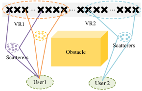
Figure 1: Illustration of spatial non-stationarity in XL-MIMO systems

In XL-MIMO systems, the large-aperture array results in a more significant Rayleigh distance, causing the transmission to occur in the near-field region [7, 8, 9]. Consequently, the planar wavefront assumption used in far-field communications becomes invalid, as the wavefront curvature over the array is no longer negligible. Additionally, due to obstacles and incomplete scattering, spatial non-stationarity (SnS) may appear along the array [10, 11, 12, 13]. Specifically, different portions of the array may observe different users, as the energy of each user is focused on a particular portion of the array, referred to as the visibility region (VR), as shown in Fig. 1.

The presence of spherical wavefront effects and SnS in XL-MIMO systems opens up new possibilities for spatial multiplexing and random access (RA). On one hand, due to the non-negligible wavefront curvature over the array, XL-MIMO channels exhibit a high-rank property, even in a line-of-sight (LoS) scenario, thereby enabling the transmission of multiple data streams [1, 14, 15, 16, 17]. For example, in our previous work [1], we evaluated the high-rank characteristic and the structured sparsity of LoS XL-MIMO channels in the wavenumber domain. Additionally, the authors of [17] proposed reconfigurable uniform linear array (ULA) schemes that employed rotating transceiver ULAs to adapt the spatial degrees of freedom (DoFs) in the case of different signal-to-noise ratio (SNR) and enhance system performance. On the other hand, SnS offers a unique advantage in improving RA performance, particularly in crowded user scenarios. Specifically, the authors of [18] introduced a non-overlapping VR RA protocol, which schedules users with non-overlapping VRs in the same payload pilot resource, allowing for the simultaneous access of more users. However, it is crucial to emphasize that these advantages heavily depend on the availability of accurate channel state information (CSI).

I-A Related Works

To the best of our knowledge, it is observed that there have been a few early attempts to address the XL-MIMO channel estimation (CE) problem. Most existing works, such as [19, 20, 21, 22, 23], primarily focused on spherical wavefront effect and did not consider the issue of SnS. Specifically, the authors of [19] studied CE for XL-MIMO systems that exploits polar-domain sparsity. Based on the polar-domain codebook, on-grid and off-grid simultaneous orthogonal matching pursuit (OMP) algorithms were proposed. Moreover, the polar-domain codebook was further applied to near-field beam training [20, 21] and hybrid-field CE [22, 23]. Regrettably, overlooking SnS could result in a significant mismatch between existing CE schemes and the actual channels. If these methods are directly applied, they may fail to capture SnS, leading to a degradation in estimation performance.

To this end, the authors of [24] proposed the subarray-wise and scatterer-wise schemes to estimate the SnS channels. Nevertheless, the schemes were heuristic without exploiting the specific channel structure, such as the antenna-domain or wavenumber-domain sparsity. In addition, in the context of SnS reconfigurable intelligent surface (RIS) cascaded channels, a three-step VR detection and CE scheme was proposed in [10]. Specifically, the cascaded channel was first roughly estimated according to the method in [25], then the VR of the user was identified by exploiting the statistical characteristic of the received power across the array elements. Finally, the channel was further refined by exploiting the near-field characteristics and jointly utilizing the pilots of multiple users. However, the VR detection method based on power detection is dependent on the accuracy of CE and is sensitive to the noise level. In particular, under low SNR scenarios, this approach could experience significant performance degradation.

Taking into consideration the antenna-domain sparsity of SnS channels, the authors of [26] characterized the XL-MIMO channels with a subarray-wise Bernoulli-Gaussian distribution. Then, a bilinear message passing algorithm was proposed for joint user activity detection and CE subjected to SnS. In fact, the assumption of subarray-wise VR is ideal since the user could only view a portion of array elements in the subarray. The authors of [27] further characterized antenna-domain channels with the element-wise Bernoulli-Gaussian distribution and utilized the one-order Markov chain to capture the spatial correlation of adjacent antenna elements.

However, the above solutions only used the statistical distribution (mean and variance) to characterize the spatial-domain channel while ignoring the propagation characteristics, such as the curvature of spherical wavefront and wavenumber-domain or polar-domain sparsity, which leads to potential estimation performance degradation. Meanwhile, these methods are developed based on a full digital precoding architecture, making it challenging to extend them to a hybrid precoding architecture.

I-B Main Contributions

In this paper, we consider the joint VR detection and CE for XL-MIMO systems with the hybrid precoding architecture. Different from the existing works that only utilize the spatial-domain sparsity, we propose to fully exploit the spatial-domain and wavenumber-domain sparsity. In particular, a two-stage VR detection and CE framework is developed. The main contributions are summarized as follows.

• We first delve into the structured sparsity characteristics of SnS XL-MIMO channels in both the spatial and wavenumber domains. Specifically, in the antenna domain, the channels exhibit a block sparse structure, a direct result of SnS. Furthermore, SnS brings about a reduction in the effective array size, resulting in two significant effects: 1) the reduction of effective spatial bandwidth; 2) the extension of beamwidth. These two effects collectively contribute to the block sparsity of SnS channels in the wavenumber domain.

• Based on the observed structured sparsity, we propose a two-stage VR detection and CE framework. In the first stage, the presence of VR is detected by leveraging the sparse structure of the spatial domain channels. Specifically, we derive the visibility belief of each antenna element according to the sum-product rule. Subsequently, a VR detection-oriented message passing (VRDO-MP) algorithm is proposed to achieve approximate Bayesian inference. In the second stage, based on the estimated VR information and wavenumber-domain sparsity, the SnS channel is accurately estimated using the belief-based orthogonal matching pursuit (BB-OMP) algorithm.

• Compared to existing state-of-the-art baselines, the proposed CE algorithm exhibits superior performance thanks to the simultaneous exploitation of the structured sparsity of SnS XL-MIMO channels in both the antenna and wavenumber domains, especially in low-SNR scenarios. In addition, simulation results show that the wavenumber-domain codebook is a practical choice for SnS XL-MIMO CE in LoS or sparse scattering environments.

I-C Organization and Notations

Organization: The rest of this paper is organized as follows. In Section II, the system model is introduced. Specifically, we first derive the wavenumber-domain channel representation and then discuss the effects of SnS. Then in Section III, we propose a two-stage VR detection and CE framework. Simulations are carried out in Section IV, and the conclusions and future works are drawn in Section V.

Notations: lower-case letters, bold-face lower-case letters, and bold-face upper-case letters are used for scalars, vectors and matrices, respectively; The superscripts $\left(\cdot\right)^{\mathrm{T}}$ and $\left(\cdot\right)^{\mathrm{H}}$ stand for transpose and conjugate transpose, respectively; $\mathrm{diag}\left(x_{1},x_{2},\dotso,x_{N}\right)$ denotes an $N\times N$ diagonal matrix with $\{x_{1},x_{2},\dotso,x_{N}\}$ being its diagonal elements; $\mathbf{I}_{N}$ denotes an $N\times N$ identity matrix; $\mathbb{C}^{M\times N}$ denotes an $M\times N$ complex matrix. In addition, a random vector $x\in\mathbb{C}$ drawn from the complex Gaussian distribution with mean $x_{0}$ and variance $v$ is characterized by the probability density function $\mathcal{CN}(x;x_{0},v)={\exp\left\{-{\left|x-x_{0}\right|^{2}}/{v}\right\}}/{\pi v}$.

II System Model

In this section, we first introduce the XL-MIMO channel model and its wavenumber-domain representation. Then, we discuss the effects of SnS.

II-A XL-MIMO Channel Model

Consider a time-division-duplexing (TDD) based narrow-band XL-MIMO communication system operating in the mmWave bands, as shown in Fig. 2. The base station (BS) utilizes a hybrid precoding architecture, where the transmit array with $N$ antenna elements employs a uniform linear array (ULA) geometry that is connected to the $N_{\mathrm{rf}}$ radio frequency (RF) chains through phase shifters to serve $Q$ single-antenna users simultaneously. The antenna spacing is denoted by $d=\lambda/2$, where $\lambda$ is the wavelength.

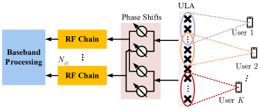
Figure 2: XL-MIMO system with hybrid precoding.

Due to the limited diffraction and severe absorption loss, the mmWave environment exhibits significantly weaker multipath propagation effects[28]. Hence, our focus primarily revolves around the LoS path. Furthermore, the combination of extremely large-scale antenna arrays and mmWave bands results in a notable increase in the Rayleigh distance, leading to users being predominantly located in the near-field region of the BS. Thus, the channel response between the $n$-th antenna element and the $q$-th user with non-uniform spherical wavefront is given by [29]

$$h_{q,n}=\frac{\lambda}{4\pi t_{q,n}}\gamma_{q}\mathrm{e}^{\mathrm{j}k_{0}t_{q,n}},$$ (1)

where $k_{0}=2\pi/\lambda$ denotes the wavenumber; $t_{q,n}=\lVert\mathbf{s}_{q}-\mathbf{r}_{n}\rVert$ is the distance between the $q$-th user and the $n$-th transmit antenna element with $\mathbf{s}_{q}=[s_{q,x},s_{q,y},s_{q,z}]^{\mathrm{T}}$ and $\mathbf{r}_{n}=[r_{n,x},r_{n,y},r_{n,z}]^{\mathrm{T}}$ indicating the corresponding coordinates, respectively; $\gamma_{q}\sim\mathcal{CN}(\gamma_{q};0,1)$ denotes the complex gain associated with the LoS path for the $q$-th user. As a result, the channel response vector $\mathbf{h}_{q}\in\mathbb{C}^{N\times 1}$ for the $q$-th user can be written as

$$\mathbf{h}_{q}=\frac{\lambda}{4\pi}\gamma_{q}\mathbf{b}(\mathbf{t}_{q}),$$ (2)

where $\mathbf{t}_{q}=[t_{q,1},t_{q,2},\cdots,t_{q,N}]^{\mathrm{T}}$ denotes the distance vector between BS and user $q$; $\mathbf{b}(\mathbf{t}_{q})$ is the array response vector with non-uniform spherical wavefront, which is denoted by

$$\mathbf{b}(\mathbf{t}_{q})=\left[\frac{\mathrm{e}^{\mathrm{j}k_{0}t_{q,1}}}{t_{q,1}},\frac{\mathrm{e}^{\mathrm{j}k_{0}t_{q,2}}}{t_{q,2}},\cdots,\frac{\mathrm{e}^{\mathrm{j}k_{0}t_{q,N}}}{t_{q,N}}\right]^{\mathrm{T}}.$$ (3)

II-B Wavenumber-Domain Channel Representation

It is intractable to analyze the property of the near-field spherical wavefront directly from (2). To this end, we decompose ${\mathrm{e}^{\mathrm{j}k_{0}t_{q,n}}}/{t_{q,n}}$ as the infinite number of plane waves traveling to different directions utilizing Weyl’s identity [30]. Since the decomposition is the same for all $Q$ users, for brevity, the subscript $q$ in the formulation (2) can be omitted. Consequently, we can obtain

$$\frac{\mathrm{e}^{\mathrm{j}k_{0}t_{n}}}{t_{n}}=\iint_{\mathcal{D}(k)}g(k_{x},k_{y};\mathbf{s})\mathrm{e}^{\mathrm{j}(k_{x}r_{n,x}+k_{y}r_{n,y})}\mathrm{d}k_{x}\mathrm{d}k_{y},$$ (4)

where $g(k_{x},k_{y};\mathbf{s})$ denotes the amplitude corresponding to the plane wave component with wave vector $\mathbf{k}=[k_{x},k_{y},k_{z}]^{\mathrm{T}}$, satisfying $k_{z}=\sqrt{k^{2}_{0}-k_{x}^{2}-k_{y}^{2}}$. Assume that the reactive propagation mechanisms are excluded, the integration region is limited to $\mathcal{D}(k)=\left\{(k_{x},k_{y}):k_{x}^{2}+k_{y}^{2}\leq k_{0}^{2}\right\}$. Particularly, in the case of ULA, the component $k_{y}$ can be omitted (assume that the array is deployed along with $x$-axis), and the wavenumber support reduces to $\mathcal{D}(k)=\left\{k_{x}:-k_{0}\leq k_{x}\leq k_{0}\right\}$.

Similar to the transition from Fourier integral to Fourier series, (4) can be discretized to finite sampling points. Assume that the size of the transmit array along the $x$-axis is denoted as $L$. In this way, the wavenumber support $\mathcal{D}(k)$ can be partitioned with spacing $\Delta=2\pi/SL$ along the $k_{x}$-axis, where $S\geq 1$ denotes the oversampling factor. By re-scaling $k_{x}$ as $k_{x}SL/2\pi$, these partitions are indexed by

$$\mathcal{S} =\left\{\xi\in\mathbb{Z}\Big{|}-1\leq\frac{\lambda\xi}{SL}<1\right\},$$ (5)

where $\xi_{i}$ indicates the $i$-th entry of $\mathcal{S}$ and corresponds to the spatial frequency component $2\pi\xi_{i}/SL$. Thus, (4) can be rewritten as

$$\frac{\mathrm{e}^{\mathrm{j}k_{0}t_{n}}}{t_{n}}\approx\sum_{i=1}^{J}g(\xi_{i};\mathbf{s})a_{R}(\xi_{i},\mathbf{r}_{n}),$$ (6)

where ${J}=\left|\mathcal{S}\right|$ is the coordinate of set $\mathcal{S}$; $g(\xi_{i};\mathbf{s})$ denotes the $i$-th decomposition coefficient. Note that the users are associated with different coefficients $g(\xi_{i};\mathbf{s})$ due to the distinctions of locations. In addition, $a_{R}(\xi_{i},\mathbf{r}_{n})$ is denoted as

$${a_{R}}(\xi_{i},\mathbf{r}_{n}) =\exp\left\{\mathrm{j}\left(\frac{2\pi}{SL}\xi_{i}r_{n,x}\right)\right\}.$$ (7)

Define vector $\mathbf{a}(\xi_{i})$ as the array response vector associated with the $i$-th spatial frequency component, which collects all the $N$ response elements, i.e.,

$$\mathbf{a}(\xi_{i}) =\frac{1}{\sqrt{N}}\left[{a}_{R}(\xi_{i},\mathbf{r}_{1}),\cdots,{a}_{R}(\xi_{i},\mathbf{r}_{N})\right]^{\mathrm{T}}.$$ (8)

Therefore, the channel response vector of the $q$-th user can be represented as

$$\mathbf{h}_{q}\approx\sqrt{N}\sum_{i=1}^{J}c_{q,i}\mathbf{a}(\xi_{i}),$$ (9)

where $c_{q,i}=\lambda\gamma_{q}g(\xi_{i};\mathbf{s}_{q})/{4\pi}$ denotes the $i$-th equivalent coefficient of the $q$-th user. Note that the random variable $c_{q,i}$ characterizes the complex gain of each plane wave component with mean zeros and variance $(\lambda g(\xi_{i};\mathbf{s}_{q})/{4\pi})^{2}$, where the variance is associated with the path loss [31].

Moreover, introduce $\cos\vartheta_{i}=2\pi\xi_{i}/SLk_{0}$ and utilize the fact that the coordinates of antenna $n$ is denoted as $\mathbf{r}_{n}=[nd,0,0]^{\mathrm{T}}$, $n\in\left\{0,1,\cdots,N-1\right\}$, and we have ${a_{R}}(\xi_{i},\mathbf{r}_{n})=\exp\left\{\mathrm{j}{\pi}\cos\vartheta_{i}n\right\}$. In this manner, (8) can be further written as

$$\mathbf{a}(\xi_{i}) =\frac{1}{\sqrt{N}}\left[1,e^{\mathrm{j}\pi\cos\vartheta_{i}},\cdots,e^{\mathrm{j}\pi\cos\vartheta_{i}(N-1)}\right]^{\mathrm{T}}.$$ (10)

Therefore, (9) can be rewritten more compactly in matrix form as

$$\mathbf{h}_{q}={\mathbf{F}}\mathbf{h}_{a,q},$$ (11)

where $\mathbf{h}_{a,q}=\sqrt{N}[c_{q,1},c_{q,2},\cdots,c_{q,J}]^{\mathrm{T}}\in\mathbb{C}^{J\times 1}$ denotes the wavenumber-domain channel vector for the $q$-th user; ${\mathbf{F}}\in\mathbb{C}^{N_{t}\times J}$ composes of the stacking array response vectors $\mathbf{a}(\xi_{i})$, $i=1,2,\cdots,J$. Note that that ${\mathbf{F}}$ is a semi-unitary matrix, which realizes the transformation from antenna domain to wavenumber domain. Therefore, ${\mathbf{F}}$ can be essentially seen as the wavenumber-domain codebook.

Due to the limited array size, only a few spatial frequency components are significant in $\mathcal{S}$, and these components usually concentrate on a specific range of spatial frequencies, which is called effective spatial bandwidth. The effective spatial bandwidth for the $q$-th user is defined as [1]

$$B_{q,e}=k_{0}\left(\max_{\mathbf{r}_{n}\in\mathcal{L}}\hat{\mathbf{r}}^{\mathrm{T}}(\mathbf{r}_{n},\mathbf{s}_{q})\hat{\mathbf{x}}-\min_{\mathbf{r}_{n}\in\mathcal{L}}\hat{\mathbf{r}}^{\mathrm{T}}(\mathbf{r}_{n},\mathbf{s}_{q})\hat{\mathbf{x}}\right),$$ (12)

where $\hat{\mathbf{r}}(\mathbf{r}_{n},\mathbf{s}_{q})=(\mathbf{r}_{n}-\mathbf{s}_{q})/\lVert\mathbf{r}_{n}-\mathbf{s}_{q}\rVert$ denotes the unit vector from $\mathbf{r}_{n}$ to $\mathbf{s}_{q}$; $\hat{\mathbf{x}}$ is the unit vector parallel to the ULA; $\mathcal{L}$ is the linear region spanned by the ULA. According to (12), we can obtain the number of effective spatial frequency components for the $q$-th user as

$$J_{q,e}\approx\lceil{B_{q,e}}/{\Delta}\rceil.$$ (13)

where $\lceil\cdot\rceil$ is to take the ceiling.

Example: For the sake of clarity, let us illustrate the wavenumber-domain of XL-MIMO channels using an example with the following parameters: $\lambda=0.01$m, $N_{t}=256$, $\mathbf{s}_{1}=[0,20\mathrm{m},0]^{\mathrm{T}}$, $\mathbf{r}_{n}=[nd,0,0]^{\mathrm{T}}$, $\forall n\in\left\{0,1,\cdots,255\right\}$, $L\approx 128\lambda$, and $S=1$. According to (5), we have $\mathcal{S}=\left\{-128,-127,\cdots,126,127\right\}$, $J=256$, and $\cos\theta_{i}=2\xi_{i}/N$. At this point, $\mathbf{F}$ becomes a $256\times 256$ DFT matrix. Additionally, using (12) and (13), we can obtain $J_{1,e}=9$.

Remark 1.

The formula (9) provides a wavenumber-domain decomposition for LoS XL-MIMO channels, which is represented as a superposition of multiple plane wave components. Due to the limited size of the array, only $J_{q,e}$ ($J_{q,e}\ll J$) components significantly contribute to the channel of the $q$-th user, which implies that the LoS XL-MIMO channels present the sparsity in wavenumber domain. In contrast to the existing polar-domain representation proposed in [19], which simultaneously samples angle- and distance-domain information, the representation presented in (11) exclusively samples in the wavenumber domain. Distance information is embedded in the effective spatial bandwidth, resulting in a more low-dimensional codebook.

II-C Effects of SnS

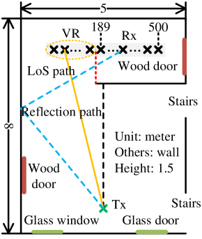
(a) Simulation Scenarios

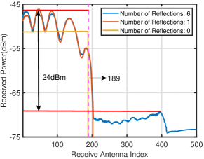
(b) Received power across elements

Figure 3: SnS simulations based on Rencom Wireless Insite Software.

Another important characteristic of XL-MIMO channels is SnS, where different users are visible to various portions of the array, as illustrated in Fig. 2. Given that an obstacle may have an arbitrary size and appear at an unpredictable location, the VR is modeled as a randomly selected subset of antenna elements for simplification. Define $\boldsymbol{\phi}_{q}\in\left\{1,2,\cdots N\right\}$ as the set of the visible antenna elements for the $q$-th user, thus, the VR indicator vector of the $q$-th user is denoted as $\boldsymbol{\alpha}_{q}\in\mathbb{Z}^{N\times 1}$, whose $n$-th element is given by

$${\alpha}_{q,n}=\left\{\begin{aligned} 1&,\quad\text{if}\ n\in\boldsymbol{\phi}_{q},\\ 0&,\quad\text{otherwise}.\\ \end{aligned}\right.$$ (14)

with

$$\psi_{q}={\left|\boldsymbol{\phi}_{q}\right|}/{N},$$ (15)

indicating the proportion of array elements visible to the $q$-th user. Then, the SnS channel $\mathbf{x}_{q}$ between BS and the $q$-th user can be written as [11, 27]

$$\mathbf{x}_{q}=\boldsymbol{\alpha}_{q}\odot\mathbf{h}_{q}=\mathrm{diag}(\boldsymbol{\alpha}_{q})\mathbf{h}_{q},$$ (16)

where $\odot$ denotes the Hadamard product.

According to (16), the SnS could result in significant variations in the average received power across antenna elements. Specifically, the received power within the VR is considerably higher than the received power outside the VR. To empirically validate this observation, we conduct simulations of SnS using Remcom Wireless Insite, a commercial 3D ray-tracing software [32]. The simulations are performed in a 5$\times$8 m indoor room, as depicted in Figure 3(a). The transmitter (Tx) and receiver (Rx) consist of omnidirectional antennas placed at a height of 1.5 m above the ground. A narrow-band sinusoidal waveform at a frequency of 28 GHz was utilized. To simulate the SnS, some of the receive array elements are obstructed by a wall, resulting in a subset of visible antenna elements denoted as $\boldsymbol{\phi}=\left\{1,2,\cdots,189\right\}$. Figure 3(b) illustrates the received power across the elements for varying numbers of reflections. When the number of reflections is small (0 or 1), the received power of the array elements outside the VR is nearly zero. Furthermore, even with an adequate number of reflections, the received power of the array elements outside the VR remains significantly lower than that of the array elements within the VR. These results confirm the effectiveness of the SnS channel model described in (16).

Fig. 4 illustrates the wavenumber-domain channels in both spatial stationary and SnS scenarios with $N=512$, $\lambda=3\times 10^{-3}$m, $\psi=0.25$, the distance between the center of ULA and user is $10$m. It is evident that both the spatial stationary and SnS XL-MIMO channels exhibit specific block sparsity. Notably, the sparsity characteristics in the two scenarios have subtle differences. The distinctions in the wavenumber-domain channels can be elaborated upon from the following two aspects:

1. Due to the presence of SnS, only a portion of the array can capture the electromagnetic wave radiated by the user. This is equivalent to reducing the effective receiving size of the array between BS and user. As described in (12), when the effective size of the array is reduced, the effective spatial bandwidth between the user and array will also be correspondingly diminished.

2. Additionally, it is noted that the decrease on the effective array size also leads to the more significant energy spread phenomenon, i.e., the beamwidth corresponding to each spatial frequency component will be extended[33].

Therefore, the block sparsity of SnS XL-MIMO channels in the wavenumber domain results from the synthesis of two factors. Specifically, when the decrease in effective spatial frequency components dominates, the wavenumber-domain channel will exhibit more pronounced sparsity, as depicted in Fig. 4. Conversely, when the energy spread phenomenon dominates, the significant components of $\mathbf{h}_{a,q}$ will further increase.

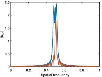
Figure 4: The wavenumber-domain channel of spatial stationary and non-stationary scenarios.

III Two-Stage VR Detection and CE Scheme

In this section, we first introduce the joint VR detection and CE scheme. Then, we formulate the VR detection as a Bayesian inference problem, which is efficiently solved using a structured MP framework in the antenna domain. Finally, leveraging the obtained VR information, the wavenumber-domain channel estimation is derived as a sparse signal recovery problem and is solved through OMP-based method.

III-A Joint VR Detection and CE Protocol

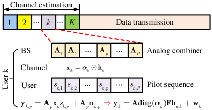
Figure 5: The proposed two-stage CE protocol

To obtain the VR information and channel coefficients, different users transmit the pilot sequence to the BS over $P$ slots. Due to the reciprocity of the TDD channel, we could only consider the uplink to formulate the VR detection and CE problems. Assume that the $Q$ users transmit mutually orthogonal pilot sequences to the BS, e.g., orthogonal time resources are utilized for different users. Denote $s_{q,p}$ as the transmit pilot of the $q$-th user in time slot $p$, as shown in Fig. 5. Then, the received pilot signal $\mathbf{y}_{q,p}\in\mathbb{C}^{N_{\mathrm{rf}}\times 1}$ in RF chains can be expressed as

$$\mathbf{y}_{q,p}=\mathbf{A}_{p}\mathbf{x}_{q}s_{q,p}+\mathbf{A}_{p}\mathbf{n}_{q,p},$$ (17)

where $\mathbf{x}_{q}$ is the spatial-domain channel response given in (16); $\mathbf{A}_{p}\in\mathbb{C}^{N_{\mathrm{rf}}\times N}$ and $\mathbf{n}_{q,p}\sim\mathcal{CN}(\mathbf{n}_{q,p};0,\sigma_{N}^{2}\mathbf{I}_{N})\in\mathbb{C}^{N\times 1}$ denote the analog combiner matrix and the complex additional white Gaussian noise (AWGN) in the $p$-th time slot, respectively; Without loss of generality, assume $s_{q,p}=1$ ($\forall q$ and $p$) and collect $P$ pilot symbol, the overall received pilot sequence $\mathbf{y}_{q}=[\mathbf{y}_{q,1}^{\mathrm{T}},\mathbf{y}_{q,2}^{\mathrm{T}},\cdots,\mathbf{y}_{q,P}^{\mathrm{T}}]^{\mathrm{T}}\in\mathbb{C}^{PN_{\mathrm{rf}}\times 1}$ for user $k$ can be denoted as

$$\mathbf{y}_{q}=\mathbf{A}\mathbf{x}_{q}+\mathbf{w}_{q},$$ (18)

where $\mathbf{A}=[\mathbf{A}_{1}^{\mathrm{T}},\mathbf{A}_{2}^{\mathrm{T}},\cdots,\mathbf{A}_{P}^{\mathrm{T}}]^{\mathrm{T}}$ $\in\mathbb{C}^{PN_{\mathrm{rf}}\times N}$ denotes the overall combiner matrix, which is composed of $M=PN_{\mathrm{rf}}$ randomly selected rows of the normalized DFT matrix, whose $(m,n)$-th entry is given by $\frac{1}{\sqrt{N}}\exp\left({\mathrm{j}\frac{2\pi(m-1)(n-1)}{N}}\right)$; $\mathbf{w}_{q}=[\mathbf{n}^{\mathrm{T}}_{q,1}\mathbf{A}_{1}^{\mathrm{T}},\mathbf{n}^{\mathrm{T}}_{q,2}\mathbf{A}_{2}^{\mathrm{T}},\cdots,\mathbf{n}^{\mathrm{T}}_{q,P}\mathbf{A}_{P}^{\mathrm{T}}]^{\mathrm{T}}\in\mathbb{C}^{PN_{\mathrm{rf}}\times 1}$ denotes the effective noise. Since $\mathbf{A}$ is a semi-unitary matrix, i.e., $\mathbf{A}\mathbf{A}^{\mathrm{H}}=\mathbf{I}_{M}$, $\mathbf{w}_{q}$ is still Gaussian noise satisfying $\mathcal{CN}(\mathbf{w}_{q};0,\sigma^{2}_{N}\mathbf{I}_{M})$. Since the orthogonal time resources are utilized for different users, we consider the $q$-th user as an example and other users can follow a similar procedure. For brevity, we omit the subscript $q$ in the following part of this subsection.

Recently, various schemes have been explored to estimate the SnS channels [10, 24, 26, 27]. However, two limitations arise with these existing methods. Firstly, in low SNR scenarios, the VR detection performance may be limited. Secondly, neglecting the spherical wavefront and wavenumber-domain sparsity might result in estimation performance degradation. To improve the VR detection and CE performance, we propose to exploit the sparsity of both the antenna and wavenumber domains in this work. Utilizing the representation in (11), the overall receive signal can be rewritten as

$$\mathbf{y}=\mathbf{A}\mathbf{x}+\mathbf{w}=\mathbf{A}\mathrm{diag}(\boldsymbol{\alpha})\mathbf{F}\mathbf{h}_{a}+\mathbf{w},$$ (19)

where $\mathbf{F}$ represents the wavenumber-domain basis used to transform the channels from the spatial domain to the wavenumber domain. Additionally, $\mathbf{A}$ denotes the overall analog combiner matrix responsible for mapping the received signals from various antenna elements to a limited number of RF chains to reduce the hardware cost.

In this paper, our goal is to estimate the user’s VR $\boldsymbol{\alpha}$ and wavenumber-domain channel $\mathbf{h}_{a}$ based on the observation vector $\mathbf{y}$. However, this estimation task faces two significant challenges. Firstly, given that the number of RF chains is much smaller than the number of antennas, the BS cannot simultaneously observe signals from all antennas, leading to unacceptable pilot overhead. Secondly, the estimation of $\boldsymbol{\alpha}$ and $\mathbf{h}_{a}$ occurs in different domains, making simultaneous estimation difficult. To solve these problems, we propose a two-stage estimation scheme. Specifically, in the first stage, our focus is on detecting the visibility region of the user, which is formulated as a Bayesian inference problem. To effectively address this problem, we introduce a structured MP framework. In the second stage, based on the extracted VR information and the wavenumber-domain sparsity, the CE is derived as a sparse signal recovery problem.

III-B Stage I: VR Detection in Antenna Domain

Due to the SnS of XL-MIMO channels, the spatial-domain channel $\mathbf{x}$ exhibits block sparsity. With some abuse of notation, we assume that the channel coefficients conditioned on VR are independent and identically distributed as Bernoulli Gaussian [27, 26], which is given by

$$p(x_{n}|\alpha_{n})=(1-\alpha_{n})\delta(x_{n})+\alpha_{n}\mathcal{CN}(x_{n};0,\sigma^{2}),$$ (20)

where $\delta(\cdot)$ denotes the Dirac delta function, which evaluates to 1 when $x=0$ and 0 otherwise; $x_{n}$ is the channel coefficient between the $n$-th antenna and the user; $\alpha_{n}$ denotes the corresponding visibility indicator. According to (20), it is evident that when the antenna element $n$ is invisible to the user, indicated by $\alpha_{n}=0$, the channel coefficient $x_{n}$ is zero. Otherwise, when $\alpha_{n}=1$, the channel coefficient $x_{n}$ follows a Gaussian distribution with mean zero and variance $\sigma^{2}$.

In practical scenarios, the VR of the user shows spatial correlation among the adjacent antennas. This implies that the non-zero elements of $\boldsymbol{\alpha}$ tend to concentrate within a specific portion of the antenna elements. To effectively capture this spatial correlation, a block-sparse structure can be employed, which can be characterized using a one-order Markov chain as

$$p(\boldsymbol{\alpha})=p(\alpha_{1})\prod_{n=2}^{N}p(\alpha_{n}|\alpha_{n-1}),$$ (21)

where the steady state probability of Markov chain is given by $p(\alpha_{n}=1)=\psi$, where $\psi$ is defined in (15) and reflects the sparsity of the antenna-domain channel. The transition probability of Markov chain $p(\alpha_{n}|\alpha_{n-1})$, $n=2,3,\cdots,N$, is given by

$$p(\alpha_{n}|\alpha_{n-1})=\left\{\begin{aligned} (1-p_{01})^{1-\alpha_{n}}p_{01}^{\alpha_{n}}&,\quad\alpha_{n-1}=0,\\ p_{10}^{1-\alpha_{n}}(1-p_{10})^{\alpha_{n}}&,\quad\alpha_{n-1}=1,\\ \end{aligned}\right.$$ (22)

where $p_{01}=p(\alpha_{n}=0|\alpha_{n-1}=1)$ and other three transition probabilities are defined similarly. With the steady-state assumption, the Markov chain can be completely characterized by two parameters $\psi$ and $p_{10}$. The other three transition probabilities can be easily obtained as $p_{01}=\psi p_{10}/(1-\psi)$, $p_{00}=1-p_{01}$, and $p_{11}=1-p_{10}$.

Combining the prior distribution provided in (20) and (21), the probabilistic signal model describing the problem in (19) can be derived as

$$p(\mathbf{y},\mathbf{x},\boldsymbol{\alpha})=p(\mathbf{y}|\mathbf{x},\boldsymbol{\alpha})p(\mathbf{x}|\boldsymbol{\alpha})p(\boldsymbol{\alpha}),$$ (23)

where the conditional probability $p(\mathbf{y}|\mathbf{x},\boldsymbol{\alpha})$ is obtained from the AWGN channel as

$$p(\mathbf{y}|\mathbf{x},\boldsymbol{\alpha})=\frac{1}{\pi\sigma_{N}^{2}}\exp\left(-\frac{\lVert\mathbf{y-Ax}\rVert^{2}}{\sigma_{N}^{2}}\right).$$ (24)

Based on the probabilistic model provided in (23), the optimal detection of VR in terms of the minimum mean square error (MMSE) principle can be realized by Bayesian inference. Specifically, the posterior probability $\boldsymbol{\alpha}$ is given by

$$p(\boldsymbol{\alpha},\mathbf{x}|\mathbf{y})=\frac{p(\boldsymbol{\alpha},\mathbf{x},\mathbf{y})}{p(\mathbf{y})}\propto p(\boldsymbol{\alpha},\mathbf{x},\mathbf{y}).$$ (25)

Thus, the VR detection can be formulated as a posterior estimation problem, i.e.,

$$\hat{\boldsymbol{\alpha}}\propto\mathop{\arg\max}\limits_{\boldsymbol{\alpha}}p(\mathbf{y}|\mathbf{x},\boldsymbol{\alpha})p(\mathbf{x}|\boldsymbol{\alpha})p(\boldsymbol{\alpha}).$$ (26)

By comparing (26) with a predefined threshold, the antenna visibility can be accurately decided.

Due to the fact that the number of antenna elements in XL-MIMO systems is extremely large, it is computationally intractable to obtain the exact solution of (26). Recently, approximate message passing (AMP) techniques [34, 35, 36] with low complexity have been extensively utilized for the maximum posterior (MAP) estimation problem. For example, based on the generalized approximate message passing (GAMP) method [34, 35], the work in [36] proposed a novel bilinear message-scheduling GAMP, that jointly performs device activity detection, channel estimation and data decoding in a grant-free massive MIMO scenario. Inspired by the superiority of MP in MAP estimation, we propose to utilize the structured MP framework to approximately extract the VR. Specifically, the VR detection-orientated MP (VRDO-MP) framework decouples the original problem (26) into two MMSE estimators as shown in Fig. 6:

• Module A: linear MMSE estimator of $\mathbf{x}$, which is decoupled from the observation $\mathbf{y}$ by exploiting the likelihood $p(\mathbf{y}|\mathbf{x},\boldsymbol{\alpha})$ and the messages from Module B;

• Module B: VR detector of $\boldsymbol{\mathbf{\alpha}}$, where $\boldsymbol{\mathbf{\alpha}}$ is estimated by combining the structured priors $p(\mathbf{x}|\boldsymbol{\alpha})$, $p(\boldsymbol{\alpha})$ and the output message from Module A.

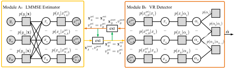
Figure 6: The block diagram of the proposed structured message passing.

Since the information of VR is implicit in $\mathbf{x}$, Module A and Module B utilize $\mathbf{x}$ as a bridge for message passing. Fig. 6 also depicts the factor graph corresponding to the probabilistic model presented in (26), where the likelihood and prior are represented as factor nodes (gray rectangles), while the random variables are represented as variable nodes (blank circles), and the gray circles indicate the observed values.

III-B1 LMMSE Estimator

In Module A, the antenna-domain channel $\mathbf{x}$ is estimated based on the received pilot vector $\mathbf{y}$ and the prior distribution $\mathcal{CN}(\mathbf{x};\mathbf{x}_{A}^{\mathrm{pri}},v_{A}^{\mathrm{pri}})$, where $\mathbf{x}_{A}^{\mathrm{pri}}$ and $v_{A}^{\mathrm{pri}}$ are extrinsic inputs from Module B, which is elaborated later. Given the received pilot sequence $\mathbf{y}$ and prior distribution of $\mathbf{x}$, the posterior mean and the mean-square error (MSE) matrix of $\mathbf{x}$ are respectively derived by using LMMSE rule as [37]

$$\mathbf{x}_{A}^{\mathrm{post}} =\mathbf{x}_{A}^{\mathrm{pri}}+v_{A}^{\mathrm{pri}}\mathbf{A}^{\mathrm{H}}\left(v_{A}^{\mathrm{pri}}\mathbf{A}\mathbf{A}^{\mathrm{H}}+\sigma_{N}^{2}\mathbf{I}_{M}\right)^{-1}(\mathbf{y}-\mathbf{A}\mathbf{x}_{A}^{\mathrm{pri}})$$ (27)

$$\overset{(a)}{=}\mathbf{x}_{A}^{\mathrm{pri}}+\frac{v_{A}^{\mathrm{pri}}}{v_{A}^{\mathrm{pri}}+\sigma_{N}^{2}}\mathbf{A}^{\mathrm{H}}(\mathbf{y}-\mathbf{A}\mathbf{x}_{A}^{\mathrm{pri}}),$$

$$\mathbf{V}_{A}^{\mathrm{post}} =v_{A}^{\mathrm{pri}}{\mathbf{I}_{N}}-(v_{A}^{\mathrm{pri}})^{2}\mathbf{A}^{\mathrm{H}}\left(v_{A}^{\mathrm{pri}}\mathbf{A}\mathbf{A}^{\mathrm{H}}+\sigma_{N}^{2}\mathbf{I}_{M}\right)^{-1}\mathbf{A}$$ (28)

$$\overset{(b)}{=}\left(v_{A}^{\mathrm{pri}}-\frac{M}{N}\frac{(v_{n,A}^{\mathrm{pri}})^{2}}{v_{n,A}^{\mathrm{pri}}+\sigma_{N}^{2}}\right)\mathbf{I}_{N}.$$

where $(a)$ and $(b)$ are obtained due to $\mathbf{A}^{\mathrm{H}}\mathbf{A}=(M/N)\mathbf{I}_{N}$ and $\mathbf{A}{\mathbf{A}^{\mathrm{H}}}=\mathbf{I}_{M}$.

Then, the extrinsic outputs of Module A are respectively given by [27, 38]

$$v_{A}^{\mathrm{ext}} =\left({1}/{v_{A}^{\mathrm{post}}}-{1}/{v_{A}^{\mathrm{pri}}}\right)^{-1},$$ (29)

$$\mathbf{x}_{A}^{\mathrm{ext}} =v_{A}^{\mathrm{ext}}\left({\mathbf{x}_{A}^{\mathrm{post}}}/{v_{A}^{\mathrm{post}}}-{\mathbf{x}_{A}^{\mathrm{pri}}}/{v_{A}^{\mathrm{pri}}}\right).$$ (30)

Meanwhile, the extrinsic outputs of Module A serve as the approximate likelihood to Module B, i.e., $\mathbf{x}_{B}^{\mathrm{pri}}=\mathbf{x}_{A}^{\mathrm{ext}}$, ${v}_{B}^{\mathrm{pri}}=v_{A}^{\mathrm{ext}}$.

III-B2 VR Detector

To begin with, the input messages of Module B, $\mathbf{x}_{B}^{\mathrm{pri}}$, are characterized as an additive white Gaussian noise observation [39], i.e., $\mathbf{x}_{B}^{\mathrm{pri}}=\mathbf{x}+\mathbf{z}$, where $\mathbf{z}\sim\mathcal{CN}(\mathbf{z};0,{v}_{B}^{\mathrm{pri}}\mathbf{I}_{N})$ is independent of $\mathbf{x}$, and ${v}_{B}^{\mathrm{pri}}$ is the input variance from Module A. Therefore, the observation variable nodes $\{y_{m}\}$ of factor graph in Fig. 6 are replaced by $\{{x}_{n,B}^{\mathrm{pri}}\}$, and the factor nodes $\{p(y_{m}|\mathbf{x})\}$ are replaced by $\{p(x_{n,B}^{\mathrm{pri}}|x_{n})\}$. In this manner, we have

$$p(x_{n,B}^{\mathrm{pri}}|x_{n})=\mathcal{CN}(x_{n,B}^{\mathrm{pri}};x_{n},v_{B}^{\mathrm{pri}}).$$ (31)

Then, we will derive the message passing process in Module B. The definitions of involved messages for Module B are summarized in TABLE. I. According to the sum-product rules, message updates are presented as follows.

TABLE I: Message Definition for Module B

Notation	Definition	Distribution
$\nu_{x_{n}\rightarrow p(x_{n}|\alpha_{n})}(x_{n})$	message from $x_{n}$ to $p(x_{n}|\alpha_{n})$	$\mathcal{CN}(x_{n};x_{n,B}^{\mathrm{pri}},v_{n,B}^{\mathrm{pri}})$
$\nu_{p(x_{n}|\alpha_{n})\rightarrow\alpha_{n}}(\alpha_{n})$	message from $p(x_{n}|\alpha_{n})$ to $\alpha_{n}$	$\pi_{n}^{\mathrm{out}}\delta(1-\alpha_{n})+(1-\pi_{n}^{\mathrm{out}})\delta(\alpha_{n})$
$\nu_{\alpha_{n}\rightarrow p(\alpha_{n+1}|\alpha_{n})}$	message from $\alpha_{n}$ to $p(\alpha_{n+1}|\alpha_{n})$	$\lambda^{f}_{n}\pi_{n}^{\mathrm{out}}\delta(1-\alpha_{n})+(1-\lambda^{f}_{n})(1-\pi_{n}^{\mathrm{out}})\delta(\alpha_{n})$
$\nu_{p(\alpha_{n}|\alpha_{n-1})\rightarrow\alpha_{n}}(\alpha_{n})$	message from $p(\alpha_{n}|\alpha_{n-1})$ to $\alpha_{n}$	$(1-\lambda^{f}_{n-1})(1-\pi_{n-1}^{\mathrm{out}})p(\alpha_{n}|\alpha_{n-1}=0)$ $+\lambda^{f}_{n-1}\pi_{n-1}^{\mathrm{out}}p(\alpha_{n}|\alpha_{n-1}=1)$
$\nu_{\alpha_{n}\rightarrow p(\alpha_{n}|\alpha_{n-1})}(\alpha_{n})$	message from $\alpha_{n}$ to $p(\alpha_{n}|\alpha_{n-1})$	$\lambda^{b}_{n}\pi_{n}^{\mathrm{out}}\delta(1-\alpha_{n})+(1-\lambda^{b}_{n})(1-\pi_{n}^{\mathrm{out}})\delta(\alpha_{n})$
$\nu_{p(\alpha_{n+1}|\alpha_{n})\rightarrow\alpha_{n}}(\alpha_{n})$	message from $p(\alpha_{n+1}|\alpha_{n})$ to $\alpha_{n}$	$(1-\lambda^{b}_{n+1})(1-\pi_{n+1}^{\mathrm{out}})p(\alpha_{n+1}=0|\alpha_{n})$ $+\lambda^{b}_{n+1}\pi_{n+1}^{\mathrm{out}}p(\alpha_{n+1}=1|\alpha_{n})$
$\nu_{\alpha_{n}\rightarrow p(x_{n}|\alpha_{n})}(\alpha_{n})$	message from $\alpha_{n}$ to $p(x_{n}|\alpha_{n})$	$\pi^{\mathrm{in}}_{n}\delta(1-\alpha_{n})+(1-\pi^{\mathrm{in}}_{n})\delta(\alpha_{n})$
$\nu_{p(x_{n}|\alpha_{n})\rightarrow x_{n}}(x_{n})$	message from $p(x_{n}|\alpha_{n})$ to $x_{n}$	$\pi^{\mathrm{in}}_{n}\mathcal{CN}(x_{n};0,\sigma^{2})+(1-\pi^{\mathrm{in}}_{n})\delta(x_{n})$
$\mathcal{M}(\alpha_{n})$	message from $p(y_{m}|\mathbf{x})$ to $x_{n}$	$\lambda_{n}^{\mathrm{post}}\delta(1-\alpha_{n})+(1-\lambda_{n}^{\mathrm{post}})\delta(\alpha_{n})$

• The message from variable node $x_{n}$ to factor node $p(x_{n}|\alpha_{n})$ is given by

  $$\nu_{x_{n}\rightarrow p(x_{n}|\alpha_{n})}(x_{n})=\mathcal{CN}(x_{n};x_{n,B}^{\mathrm{pri}},v_{n,B}^{\mathrm{pri}}).$$ (32)

• The message from factor node $p(x_{n}|\alpha_{n})$ to variable node $\alpha_{n}$ is written as

  $$\nu_{p(x_{n}|\alpha_{n})\rightarrow\alpha_{n}}(\alpha_{n})$$ (33)

  $$= \int\nu_{x_{n}\rightarrow p(x_{n}|\alpha_{n})}(x_{n})p(x_{n}|\alpha_{n})\mathrm{d}x_{n}$$

  $$\propto \pi_{n}^{\mathrm{out}}\delta(1-\alpha_{n})+(1-\pi_{n}^{\mathrm{out}})\delta(\alpha_{n}),$$

  where

  $$\pi_{n}^{\mathrm{out}} =\frac{d_{n}}{\mathcal{CN}(0;x_{n,B}^{\mathrm{pri}},v_{n,B}^{\mathrm{pri}})+d_{n}},$$ (34)

  with

  $$d_{n}\triangleq\mathcal{CN}(0;x_{n,B}^{\mathrm{pri}},\sigma^{2}+v_{n,B}^{\mathrm{pri}}).$$ (35)

  Proof.

  see Appendix A. ∎

• Denote $\psi^{f}_{n}$ as the forward message passing of Markov chain from $p(\alpha_{n}|\alpha_{n-1})$ to $\alpha_{n}$, i.e., $\nu_{p(\alpha_{n}|\alpha_{n-1})\rightarrow\alpha_{n}}(\alpha_{n})=\psi^{f}_{n}\delta(1-\alpha_{n})+(1-\psi^{f}_{n})\delta(\alpha_{n}),\forall n\geq 2$. For $n=1$, we always have $\nu_{p(\alpha_{n}|\alpha_{n-1})\rightarrow\alpha_{n}}(\alpha_{n})=\psi\delta(1-\alpha_{n})+(1-\psi)\delta(\alpha_{n})$, since $p(\alpha_{1})$ is only connected with $\alpha_{1}$ in the factor graph [27, 38]. Then, the message from variable node $\alpha_{n}$ to factor node $p(\alpha_{n+1}|\alpha_{n})$ is written as

  $$\nu_{\alpha_{n}\rightarrow p(\alpha_{n+1}|\alpha_{n})}(\alpha_{n})$$ (36)

  $$= \nu_{p(x_{n}|\alpha_{n})\rightarrow\alpha_{n}}(\alpha_{n})\nu_{p(\alpha_{n}|\alpha_{n-1})\rightarrow\alpha_{n}}(\alpha_{n})$$

  $$= \psi^{f}_{n}\pi_{n}^{\mathrm{out}}\delta(1-\alpha_{n})+(1-\psi^{f}_{n})(1-\pi_{n}^{\mathrm{out}})\delta(\alpha_{n}).$$

• The message from factor node $p(\alpha_{n}|\alpha_{n-1})$ to variable node $\alpha_{n}$ is given by

  $$\nu_{p(\alpha_{n}|\alpha_{n-1})\rightarrow\alpha_{n}}(\alpha_{n})$$ (37)

  $$= \int\nu_{\alpha_{n-1}\rightarrow p(\alpha_{n}|\alpha_{n-1})}(\alpha_{n-1})p(\alpha_{n}|\alpha_{n-1})\mathrm{d}\alpha_{n-1}$$

  $$= (1-\psi^{f}_{n-1})(1-\pi_{n-1}^{\mathrm{out}})p(\alpha_{n}|\alpha_{n-1}=0)$$

  $$+ \psi^{f}_{n-1}\pi_{n-1}^{\mathrm{out}}p(\alpha_{n}|\alpha_{n-1}=1).$$

  Thus, we have

  $$\psi^{f}_{n}=\frac{p_{01}(1-\psi^{f}_{n-1})(1-\pi_{n-1}^{\mathrm{out}})+p_{11}\lambda^{f}_{n-1}\pi_{n-1}^{\mathrm{out}}}{(1-\psi^{f}_{n-1})(1-\pi_{n-1}^{\mathrm{out}})+\psi^{f}_{n-1}\pi_{n-1}^{\mathrm{out}}}.$$ (38)

• Denote $\psi^{b}_{n}$ as the backward message passing of Markov chain from $p(\alpha_{n+1}|\alpha_{n})$ to $\alpha_{n}$, i.e., $\nu_{p(\alpha_{n+1}|\alpha_{n})\rightarrow\alpha_{n}}(\alpha_{n})=\psi^{b}_{n}\delta(1-\alpha_{n})+(1-\psi^{f}_{n})\delta(\alpha_{n})$, $\forall n\leq N-1$. For $n=N$, we always have $\psi^{b}_{N}=1/2$. Then, the message from variable node $\alpha_{n}$ to factor node $p(\alpha_{n}|\alpha_{n-1})$ is written as

  $$\nu_{\alpha_{n}\rightarrow p(\alpha_{n}|\alpha_{n-1})}(\alpha_{n})$$ (39)

  $$= \nu_{p(x_{n}|\alpha_{n})\rightarrow\alpha_{n}}(\alpha_{n})\nu_{p(\alpha_{n+1}|\alpha_{n})\rightarrow\alpha_{n}}(\alpha_{n})$$

  $$= \psi^{b}_{n}\pi_{n}^{\mathrm{out}}\delta(1-\alpha_{n})+(1-\psi^{b}_{n})(1-\pi_{n}^{\mathrm{out}})\delta(\alpha_{n}).$$

• The message from $p(\alpha_{n+1}|\alpha_{n})$ to $\alpha_{n}$ is given by

  $$\nu_{p(\alpha_{n+1}|\alpha_{n})\rightarrow\alpha_{n}}(\alpha_{n})$$ (40)

  $$= \int\nu_{\alpha_{n+1}\rightarrow p(\alpha_{n+1}|\alpha_{n})}(\alpha_{n+1})p(\alpha_{n+1}|\alpha_{n})\mathrm{d}\alpha_{n+1}$$

  $$= (1-\psi^{b}_{n+1})(1-\pi_{n+1}^{\mathrm{out}})p(\alpha_{n+1}=0|\alpha_{n})$$

  $$+ \psi^{b}_{n+1}\pi_{n+1}^{\mathrm{out}}p(\alpha_{n+1}=1|\alpha_{n}).$$

  Thus, we obtain (41) shown in the top of next page.

  $$\psi^{b}_{n}=\frac{p_{10}(1-\psi^{b}_{n+1})(1-\pi_{n+1}^{\mathrm{out}})+p_{11}\psi^{b}_{n+1}\pi_{n+1}^{\mathrm{out}}}{(p_{10}+p_{00})(1-\psi^{b}_{n+1})(1-\pi_{n+1}^{\mathrm{out}})+(p_{11}+p_{01})\psi^{b}_{n+1}\pi_{n+1}^{\mathrm{out}}}.$$ (41)

• The message from $\alpha_{n}$ to $p(x_{n}|\alpha_{n})$ is given by

  $$\nu_{\alpha_{n}\rightarrow p(x_{n}|\alpha_{n})}(\alpha_{n})$$ (42)

  $$= \nu_{p(\alpha_{n}|\alpha_{n-1})\rightarrow\alpha_{n}}(\alpha_{n})\nu_{p(\alpha_{n+1}|\alpha_{n})\rightarrow\alpha_{n}}(\alpha_{n})$$

  $$= \lambda^{f}_{n}\lambda^{b}_{n}\delta(1-\alpha_{n})+(1-\psi^{f}_{n})(1-\psi^{b}_{n})\delta(\alpha_{n})$$

  $$\propto \pi^{\mathrm{in}}_{n}\delta(1-\alpha_{n})+(1-\pi^{\mathrm{in}}_{n})\delta(\alpha_{n}),$$

  where $\pi^{\mathrm{in}}_{n}$ is defined as

  $$\pi^{\mathrm{in}}_{n}=\frac{\psi^{f}_{n}\psi^{b}_{n}}{\psi^{f}_{n}\psi^{b}_{n}+(1-\psi^{f}_{n})(1-\psi^{b}_{n})}.$$ (43)

• The message from $p(x_{n}|\alpha_{n})$ to $x_{n}$ is written as

  $$\nu_{p(x_{n}|\alpha_{n})\rightarrow x_{n}}(x_{n})$$ (44)

  $$= \int\nu_{\alpha_{n}\rightarrow p(x_{n}|\alpha_{n})}(\alpha_{n})p(x_{n}|\alpha_{n})\mathrm{d}\alpha_{n}$$

  $$= \pi^{\mathrm{in}}_{n}\mathcal{CN}(x_{n};0,\sigma^{2})+(1-\pi^{\mathrm{in}}_{n})\delta(x_{n}).$$

To realize the message passing from Module B to Module A and detect the VR of the user, we further elaborate the posteriori distribution of $\mathbf{x}$ and the belief of $\boldsymbol{\alpha}$ in Module B. Utilizing (36) and (48), the posteriori mean $x_{n,B}^{\mathrm{post}}=\mathbb{E}\left\{x_{n}|x_{n,B}^{\mathrm{pri}}\right\}$ of $x_{n}$ are given by

$$x_{n,B}^{\mathrm{post}}=\mathbb{E}\left\{x_{n}|x_{n,B}^{\mathrm{pri}}\right\}=\frac{a_{n}x_{n,B}^{\mathrm{pri}}}{1+b_{n}q_{n}},$$ (45)

where $a_{n}$, $b_{n}$, $c_{n}$ and $q_{n}$ are intermediate variables, satisfying $a_{n}={\sigma^{2}}/({v_{n,B}^{\mathrm{pri}}+\sigma^{2}})$, $b_{n}={(1-\pi^{\mathrm{in}}_{n})(v_{n,B}^{\mathrm{pri}}+\sigma^{2})}/{\pi^{\mathrm{in}}_{n}v_{n,B}^{\mathrm{pri}}}$, $c_{n}={\sigma^{2}}/{v_{n,B}^{\mathrm{pri}}(\sigma^{2}+v_{n,B}^{\mathrm{pri}})}$, and $q_{n}=\exp(-c_{n}|x_{n,B}^{\mathrm{pri}}|^{2})$.

Proof.

see Appendix B. ∎

Similarly, the posterior variance $v_{n,B}^{\mathrm{post}}=\mathbb{V}\mathrm{ar}\left\{x_{n}|x_{n,B}^{\mathrm{pri}}\right\}$ of $x_{n}$ are given by

$$v_{n,B}^{\mathrm{post}} =\mathbb{V}\mathrm{ar}\left\{x_{n}|x_{n,B}^{\mathrm{pri}}\right\}=b_{n}q_{n}\left|x_{n,B}^{\mathrm{post}}\right|^{2}+\frac{v_{n,B}^{\mathrm{pri}}}{x_{n,B}^{\mathrm{pri}}}x_{n,B}^{\mathrm{post}},$$ (46)

$$v_{B}^{\mathrm{post}} =\frac{1}{N}\sum_{n=1}^{N}v_{n,B}^{\mathrm{post}}.$$ (47)

With the above posterior mean and variance, the extrinsic outputs of Module B can be obtained as follows

$$v_{B}^{\mathrm{ext}} =\left({1}/{v_{B}^{\mathrm{post}}}-{1}/{v_{B}^{\mathrm{pri}}}\right)^{-1},$$ (48)

$$\mathbf{x}_{B}^{\mathrm{ext}} =v_{B}^{\mathrm{ext}}\left({\mathbf{x}_{B}^{\mathrm{post}}}/{v_{B}^{\mathrm{post}}}-{\mathbf{x}_{B}^{\mathrm{post}}}/{v_{B}^{\mathrm{pri}}}\right).$$ (49)

Combining the message from the Markov chain and factor node $p(x_{n}|\alpha_{n})$, the belief of $\alpha_{n}$ is denotes by (50) where

$$\mathcal{M}(\alpha_{n})\propto \nu_{p(x_{n}|\alpha_{n})\rightarrow\alpha_{n}}(\alpha_{n})\nu_{p(\alpha_{n}|\alpha_{n-1})\rightarrow\alpha_{n}}(\alpha_{n})\nu_{p(\alpha_{n+1}|\alpha_{n})\rightarrow\alpha_{n}}(\alpha_{n})$$ (50)

$$= \pi_{n}^{\mathrm{out}}\lambda^{f}_{n}\lambda^{b}_{n}\delta(1-\alpha_{n})+(1-\pi_{n}^{\mathrm{out}})(1-\lambda^{f}_{n})(1-\lambda^{b}_{n})\delta(\alpha_{n})$$

$$\propto \lambda_{n}^{\mathrm{post}}\delta(1-\alpha_{n})+(1-\lambda_{n}^{\mathrm{post}})\delta(\alpha_{n}),$$

$$\psi_{n}^{\mathrm{post}}=\frac{\pi_{n}^{\mathrm{out}}\psi^{f}_{n}\psi^{b}_{n}}{\pi_{n}^{\mathrm{out}}\psi^{f}_{n}\psi^{b}_{n}+(1-\pi_{n}^{\mathrm{out}})(1-\psi^{f}_{n})(1-\psi^{b}_{n})},$$ (51)

with $\psi_{n}^{\mathrm{post}}$ indicating that the estimates of the probability that the $n$-th antenna is visible. If $\psi_{n}^{\mathrm{post}}$ is greater than a threshold, the $n$-th antenna is regarded as being visible, i.e.,

$$\hat{{\alpha}}_{n}=\left\{\begin{aligned} 1&,\quad\psi_{n}^{\mathrm{post}}>\psi_{\mathrm{th}},\\ 0&,\quad\psi_{n}^{\mathrm{post}}\leq\psi_{\mathrm{th}}.\end{aligned}\right.$$ (52)

where $\psi_{\mathrm{th}}$ is a predetermined threshold.

Algorithm 1 VRDO-MP Algorithm

1:the received vector $\mathbf{y}$ and pilot matrix $\mathbf{A}$;

2:Initialize: $\mathbf{x}_{A}^{\mathrm{pri}}\leftarrow\mathbf{0}$, $v_{A}^{\mathrm{pri}}\leftarrow 1$, and $\boldsymbol{\vartheta}$.

3:while the stopping criterion is not met do

4:/*Module A: LMMSE Estimator of $x_{n}$*/

5:     Update $\mathbf{x}_{A}^{\mathrm{post}}$ and $v_{A}^{\mathrm{post}}$ by (27) and (28);

6:     Update $\mathbf{x}_{A}^{\mathrm{ext}}$ and $v_{A}^{\mathrm{ext}}$ by (29) and (30);

7:     Update $\mathbf{x}_{B}^{\mathrm{pri}}$ and ${v}_{B}^{\mathrm{pri}}$ by $\mathbf{x}_{B}^{\mathrm{pri}}\leftarrow\mathbf{x}_{A}^{\mathrm{ext}}$ and ${v}_{B}^{\mathrm{pri}}\leftarrow{v}_{A}^{\mathrm{ext}}$;

8:/*Module B: Detector of $\alpha_{n}$*/

9:     Update the message $\nu_{x_{n}\rightarrow p(x_{n}|\alpha_{n})}(x_{n})$ by (32);

10:     Update the message $\nu_{p(x_{n}|\alpha_{n})\rightarrow\alpha_{n}}(\alpha_{n})$ by (33) and (34);

11:     Update the forward message passing of Markov chain by (36) and (38);

12:     Update the backward message passing of Markov chain by (39) and (41);

13:     Update $\nu_{\alpha_{n}\rightarrow p(x_{n}|\alpha_{n})}$ by (42) and (43);

14:     Update $\nu_{p(x_{n}|\alpha_{n})\rightarrow x_{n}}$ by (44);

15:     Calculate $x_{n,B}^{\mathrm{post}}$ and $v_{B}^{\mathrm{post}}$ by (45)-(47);

16:     Update $\mathbf{x}_{B}^{\mathrm{ext}}$ and $v_{B}^{\mathrm{ext}}$ by (48) and (49);

17:     Update $\mathbf{x}_{A}^{\mathrm{pri}}$ and ${v}_{A}^{\mathrm{pri}}$ by $\mathbf{x}_{A}^{\mathrm{pri}}\leftarrow\mathbf{x}_{B}^{\mathrm{ext}}$ and ${v}_{A}^{\mathrm{pri}}\leftarrow{v}_{B}^{\mathrm{ext}}$;

18:/*Parameters learning*/

19:     Update hyperparameter $\boldsymbol{\vartheta}$ by the EM algorithm in [40, Algorithm 2];

20:end while

21:/*Estimation of $\alpha_{n}$*/

22:Calculate $\psi_{n}^{\mathrm{post}}$ and $\hat{\boldsymbol{\alpha}}$ by (51) and (52).

23:the visibility probability $\boldsymbol{\psi}_{\mathrm{post}}$ and VR $\hat{\boldsymbol{\alpha}}$

The VRDO-MP algorithm requires the prior knowledge of the system statistics characterized by the hyperparameter set $\boldsymbol{\vartheta}=\{\sigma^{2},\sigma_{N}^{2},\psi,p_{10}\}$, where $\sigma^{2}$ is the variance of spatial-domain channels, $\sigma_{N}^{2}$ is the noise variance, $\psi$ is sparse level of spatial-domain channels and $p_{01}$ is the state transition probability from $\alpha_{n}=0$ to $\alpha_{n}=1$. Unfortunately, they may not be estimated accurately in advance. To this end, we propose to integrate the EM algorithm into the VRDO-MP algorithm, where the statistical parameters are learned from the received signals during the estimation procedure. Interested readers please refer to [40, Section V] for the detailed derivation of the EM algorithm. The overall algorithm is summarized in Algorithm 1.

III-C Stage II: CE in Wavenumber Domain

Algorithm 2 Proposed belief-Based OMP (BB-OMP) Algorithm

the received vector $\mathbf{y}$ and pilot matrix $\mathbf{A}$, $\boldsymbol{\lambda}^{\mathrm{post}}$, $\mathbf{F}$, wavenumber-domain codebook $\mathbf{F}$, and the visibility probability $\boldsymbol{\lambda}_{\mathrm{post}}$;

Initialize: $\mathbf{r}_{-1}=\mathbf{0}$, $\mathbf{r}_{0}=\mathbf{y}$, $\mathcal{I}_{0}=\emptyset$, and $t=1$;

Construct the sensing matrix $\hat{\boldsymbol{\Phi}}$ by (55);

while the stopping criterion is not met do

     $j=\mathop{\arg\min}\limits_{i}\left|\hat{\boldsymbol{\Phi}}(:,i)^{H}\mathbf{r}_{t-1}\right|$, $i\in\left\{1,2,\cdots,S\right\}$;

     $\mathcal{I}_{t}=\mathcal{I}_{t-1}\cup j$;

     $\mathbf{h}_{a}^{t}=\mathop{\arg\min}\limits_{\mathbf{h}_{a}}\lVert\mathbf{y}-\hat{\boldsymbol{\Phi}}_{\mathcal{I}_{t}}\mathbf{h}_{a}\rVert_{2}$;

     $\mathbf{r}_{t}=\mathbf{y}-\hat{\boldsymbol{\Phi}}_{\mathcal{I}_{t}}\mathbf{h}_{a}^{t}$;

     $t=t+1$;

end while

$\hat{\mathbf{h}}_{a}(i)=\mathbf{h}_{a}^{t}(i)$ for $i\in\mathcal{I}_{t-1}$ and $\hat{\mathbf{h}}_{a}(i)=0$ otherwise;

$\hat{\mathbf{x}}=\mathrm{diag}(\boldsymbol{\lambda}_{\mathrm{post}})\mathbf{F}\hat{\mathbf{h}}_{a}$.

$\hat{\mathbf{x}}$

In the second stage, we attempt to estimate $\mathbf{h}_{a}$ utilizing the VR information from the first stage and wavenumber-domain sparsity. Specifically, in the second stage, we have

$$\mathbf{y}=\mathbf{A}\mathrm{diag}(\hat{\boldsymbol{\alpha}})\mathbf{F}\mathbf{h}_{a}+\mathbf{n}=\boldsymbol{\Phi}\mathbf{h}_{a}+\mathbf{n},$$ (53)

where $\boldsymbol{\Phi}=\mathbf{A}\mathrm{diag}(\boldsymbol{\alpha})\mathbf{F}$ denotes the equivalent measurement matrix. Since $\mathbf{h}_{a}$ is sparse in the wavenumber domain, the estimation problem of $\mathbf{h}_{a}$ from (53) can be derived as a sparse signal recovery problem, i.e.,

$$\hat{\mathbf{h}}_{a}=\mathop{\arg\min}\limits_{\mathbf{h}_{a}} \quad\lVert\mathbf{y}-{\boldsymbol{\Phi}}\mathbf{h}_{a}\rVert_{2}$$ (54)

$$\mathrm{s.t.} \quad\lVert\mathbf{h}_{a}\rVert_{0}=J_{e},$$

where $J_{e}\approx\lceil{B_{e}^{\mathrm{n}}}/{\Delta}\rceil$ is the spatial level of $\mathbf{h}_{a}$ in wavenumber domain with $B_{e}^{\mathrm{n}}$ indicating the effective spatial bandwidth with SnS. In addition, inspired by the soft decision in channel coding and decoding theory [36], instead of utilizing $\hat{\boldsymbol{\alpha}}$ directly, we try to use the soft information of probability $\psi_{n}^{\mathrm{post}},\forall n$ to reconstruct the equivalent measurement matrix $\hat{\boldsymbol{\Phi}}$ in (53), i.e.,

$$\hat{\boldsymbol{\Phi}}=\mathbf{A}\mathrm{diag}(\boldsymbol{\psi}^{\mathrm{post}})\mathbf{F},$$ (55)

where $\boldsymbol{\psi}^{\mathrm{post}}=[\psi_{1}^{\mathrm{post}},\psi_{2}^{\mathrm{post}},\cdots,\psi_{N}^{\mathrm{post}}]^{\mathrm{T}}$ indicates the belief of antenna visibility.

The optimization problem in (54) is a non-convex optimization with $L_{0}$ norm and is difficult to solve. To this end, we propose the belief-based OMP (BB-OMP) algorithms to solve (54). The details will be is summarized in algorithm 2. Unlike the traditional OMP method, the proposed BB-OMP algorithm is characterized by the belief-based sensing matrix, which implies the SnS of the antenna domain. Therefore, the estimation performance can be greatly improved, which will be verified by simulations in Section IV.

III-D Overall Algorithm Description

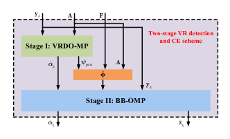
Figure 7: Illustration of the proposed two-stage VR detection and CE algorithm.

Algorithm 3 Two-Stage VR Detection and CE Algorithm

STAGE 1: Operating in antenna domain

1. input: the received vector $\mathbf{y}$ and pilot matrix $\mathbf{A}$;

2. obtain the visibility probability $\boldsymbol{\psi}_{\mathrm{post}}$ and VR $\hat{\boldsymbol{\alpha}}$ using Algorithm 1;

STAGE 2: Operating in wavenumber domain

1. input: the received vector $\mathbf{y}$, pilot matrix $\mathbf{A}$, wavenumber-domain codebook $\mathbf{F}$, and the visibility probability $\boldsymbol{\psi}_{\mathrm{post}}$;

2. obtain the channel estimate $\hat{\mathbf{x}}$ using Algorithm 2;

Outputs:

1. output: the VR $\hat{\boldsymbol{\alpha}}$;

2. the channel estimate $\hat{\mathbf{x}}$.

The two-stage VR detection and CE scheme is illustrated in Fig. 7. Specifically, the VR information $\hat{\boldsymbol{\alpha}}$ and $\boldsymbol{\psi}^{k}_{\mathrm{post}}$ is first obtained through VRDO-MP algorithm according to the observation vector $\mathbf{y}_{k}$ and analog combiner matrix $\mathbf{A}$. Subsequently, based on the obtained VR information $\boldsymbol{\psi}^{k}_{\mathrm{post}}$ and wavenumber codebook, the equivalent measurement matrix $\hat{\boldsymbol{\Phi}}$ can be obtained. Finally, the wavenumber-domain channel and corresponding spatial-domain channel can be estimated through BB-OMP algorithm. Algorithm 3 summarizes the two-stage VR detection and CE algorithm.

In the following, we provide the complexity ananlysis for Algorithm 3. Under the setting that $\mathbf{y}\in\mathbb{C}^{PN_{\mathrm{rf}}\times 1}$, $\mathbf{A}\in\mathbb{C}^{PN_{\mathrm{rf}}\times N}$, $\mathbf{F}\in\mathbb{C}^{N\times J}$, and $\mathbf{x}\in\mathbb{C}^{N\times 1}$, the complexity of VRDO-MP algorithm is elaborated as follows. In the stage I, the computational complexity for Module A per iteration is $\mathcal{O}(PN_{\mathrm{rf}}N)$. For module B, the complexity of the message passing per iteration is $\mathcal{O}(N\log N)$. Therefore, the overall complexity of Algorithm 1 is $\mathcal{O}(I_{1}PN_{\mathrm{rf}}N)$, where $I_{1}$ denotes the number of iterations in stage I. In the stage II, the computational complexity of Algorithm 2 per iteration is $\mathcal{O}(PN_{\mathrm{rf}}J)$. Thus, the overall complexity of Algorithm 3 is $\mathcal{O}(I_{1}PN_{\mathrm{rf}}N+I_{2}PN_{\mathrm{rf}}J)$, where $I_{2}$ denotes the number of iterations in stage II.

IV Simulation Results

In this section, we evaluate the performance of the proposed two-stage VR detection and CE scheme under various system setups. In particular, we consider the VR error rate (VRER) and normalized mean square error (NMSE) as performance metrics to evaluate the VR detection and CE accuracy, respectively. The VRER and NMSE are defined respectively as

$$\mathrm{VRER} \triangleq\frac{\sum_{n=1}^{N}\left|\alpha_{n}-\hat{{\alpha}}_{n}\right|}{N}\leq 1,$$ (56)

$$\mathrm{NMSE} \triangleq\frac{\lVert\hat{\mathbf{x}}-\mathbf{x}\rVert^{2}_{2}}{\lVert\mathbf{x}\lVert^{2}_{2}},$$ (57)

where $\hat{\boldsymbol{\alpha}}$ and $\hat{\mathbf{x}}$ denote the estimated channel and VR indicator vector, respectively; $\boldsymbol{\alpha}$ and ${\mathbf{x}}$ denote the true VR indicator vector and true channel vector.

The following parameters are utilized throughout the section unless specified otherwise: the number of total antenna elements $N=256$, the number of RF chains $N_{\mathrm{rf}}=4$, the carrier frequency $f_{c}=100$GHz, and the oversampling factor $S=2$. We assume that users are randomly distributed in a sector region of BS with a direction angle from $-\pi/3$ to $\pi/3$ and a distance from 5m to 50m. All the numerical results here are obtained by averaging over 5000 channel realizations.

IV-A VR Detection Performance

We utilize the rising and falling edges-based (RFEB) baseline proposed in [10] to verify the superiority of the developed VR detection algorithm. Note that the RFEB method is based on the CE result of the MJCE algorithm in [25]. However, the MJCE method cannot be applied to hybrid precoding architectures. Therefore, for comparison, we utilize the results of the least squares (LS) estimator to evaluate the performance of the RFEB method here.

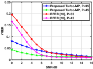
(a) $\psi=0.125$

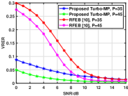
(b) $\psi=0.25$

Figure 8: VRER performance versus SNR

Fig. 8 shows the VRER performance against the SNR with the pilot lengths $P=35$ and $45$. It can be seen that the proposed VRDO-MP algorithm has superiority over the benchmark under low SNR conditions. The reason is that the VR detection method based on rising and falling edges is sensitive to the noise level. In other words, this RFEB method can easily obtain fake rising or falling edges in low SNR scenarios. Unlike the RFEB method that only utilizes the statistical characteristics of the received power, the proposed VRDO-MP fully exploits the structured block sparsity and spatial correlation through the Markov prior. Thus, the VRDO-MP detection algorithm is more robust to the noise level. Specifically, the average successful detection ratio of Turbo-MP is higher than $90\%$ with $SNR=0$dB, $P=35$, and $\psi=0.25$, while the one of RFEB is only around $70\%$, as shown in Fig. 8(b). Notably, although the detection performance of RFEB is slightly better than the proposed algorithm when $\psi=0.125$ and $SNR>8$, as shown in Fig. 8(a), the improvement is very limited or even negligible.

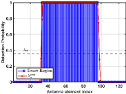
(a) Continuous visibility region

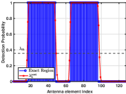
(b) Discontinuous visibility regions

Figure 9: Visibility probability of antenna elements

Moreover, Fig. 9 illustrates a realization of Monte Carlo simulation, where $SNR=5$dB, $P=45$, $\lambda=0.25$ with $\boldsymbol{\phi}=\left\{33,34,\cdots,63,64\right\}$ for Fig. 9(a), and $\boldsymbol{\phi}=\boldsymbol{\phi}^{1}\cup\boldsymbol{\phi}^{2}$ for Fig. 9(b), where $\boldsymbol{\phi}^{1}=\left\{17,18,\cdots,47,48\right\}$ and $\boldsymbol{\phi}^{2}=\left\{65,66,\cdots,95,96\right\}$. From Fig. 9(a), it is obvious that the detection probability $\lambda^{\mathrm{post}}_{n}$ is close to 1 in the VR and is close to 0 out of VR, which validates the effectiveness of the proposed detection algorithm. Moreover, the proposed detection algorithm is also feasible for discontinuous VRs, as shown in Fig. 9(b). Therefore, the proposed VR detection schemes easily expand the multi-path scenarios, where different scatters correspond to different VRs.

IV-B CE Performance

To the evaluate CE performance, we compare our proposed strategy with the following benchmarks.

• LS: Least square estimator based on the formulation (19).

• P-OMP: On-grid polar-domain simultaneous orthogonal matching pursuit algorithm for XL-MIMO channel proposed in [19] without considering VR.

• W-OMP: On-grid wavenumber-domain simultaneous orthogonal matching pursuit algorithm. Similar to P-SOMP, only the polar-domain codebook is replaced by wavenumber-domain codebook.

• AD-AMP: Antenna-domain AMP algorithm proposed in [27]. Compared with AD-AMP, the proposed algorithm operates simultaneously in the antenna and wavenumber domains to fully capture the structured sparsity of SnS XL-MIMO channels.

• Genie-aided W-SOMP. W-SOMP algorithm with perfect knowledge of VR as an absolute performance lower bound.

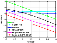
(a) NMSE versus SNR

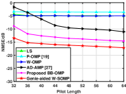
(b) NMSE versus pilot length

Figure 10: NMSE versus different estimation algorithms

To demonstrate the performance superiority of BB-SOMP, Fig. 10 compares the NMSE performance of different estimation algorithms. In particular, Fig. 10(a) provides NMSE performance against SNR, where the pilot length is $P=45$ and $\lambda=0.25$. The results show that XL-MIMO CE schemes that ignore the influence of SnS will suffer from severe performance degradation and even do not work. Therefore, the detection of VR is essential for practical CE. In addition, the proposed BB-SOMP algorithm outperforms the existing spatial-domain CE algorithm and approaches the performance bound achieved by the Genie-aided LS scheme. The reason is that compared with the antenna-domain approach proposed in [27], the proposed estimation scheme simultaneously exploits the antenna-domain and wavenumber-domain sparsity caused by the SnS. Therefore, the SnS XL-MIMO channel can be effectively estimated by the BB-SOMP algorithm.

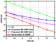
(a) $\psi=0.125$

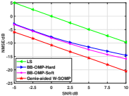
(b) $\psi=0.25$

Figure 11: NMSE versus different sensing matrices

Furthermore, the performance comparison of the proposed algorithms and the benchmarks at different pilot length $P$ is evaluated in Fig. 10(b) with $SNR=5$dB and $\psi=0.25$. The pilot sequence length $P$ increases from $32$ to $64$, so the compressive ratio $PN_{\mathrm{rf}}/N$ correspondingly increases from $0.5$ to $1$. Similarly, we can see that the proposed BB-SOMP algorithms significantly outperform the existing algorithms, especially when the pilot length is small, such as $P=36$ or $P=40$. This indicates that the proposed algorithms can significantly reduce the overhead of XL-MIMO CE.

Then, Fig. 11 investigates the estimation performance against different sensing matrices with $P=45$. Specifically, the sensing matrices are constructed by the following methods: 1) $\hat{\boldsymbol{\Phi}}=\mathbf{A}\mathrm{diag}(\boldsymbol{\lambda}^{\mathrm{post}})\mathbf{F}$; 2) $\hat{\boldsymbol{\Phi}}=\mathbf{A}\mathrm{diag}(\hat{\boldsymbol{\alpha}})\mathbf{F}$, which correspond to the BB-OMP-Soft and BB-OMP-Hard algorithms, respectively. It can be seen that the BB-SOMP-Soft always outperforms BB-SOMP-Hard algorithms due to the soft decision is more robust for the noise level. Additionally, the more sparse the channel in the antenna domain, the more obvious the performance improvement, as shown in Fig.11(a) and Fig. 11(b).

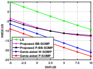
(a) $P=35$

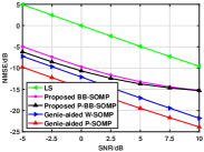
(b) $P=45$

Figure 12: NMSE performance comparison of different codebooks

Finally, inspired by the polar-main codebook proposed in [19], we also try to utilize the polar-main codebook for replacing the wavenumber-domain codebook in the formula (55) to evaluate the estimation performance. The estimation method based on the polar-domain codebook and belief of VR is called the P-BB-OMP algorithm. Figure. 12 illustrates the estimation performance comparison between the polar-domain and wavenumber-domain codebook with $\psi=0.25$. The results show that the polar-domain codebook can theoretically gain better estimation performance due to the simultaneous angle and distance sampling. However, the performance improvement is limited when the VR is not known perfectly, especially when the pilot length is small. In addition, it is noted that the size of the polar-domain codebook is much larger than the wavenumber-domain codebook. For example, when $N=256$ and $S=2$, the size of the polar-domain codebook is $2201$ [19], and the size of the wavenumber-domain codebook is only $512$. Therefore, due to their reduced dimensions and adequate estimation performance, the wavenumber-domain codebooks are a practical option for SnS XL-MIMO channels in line-of-sight or sparsely scattered scenarios.

V Conclusion and Future Works

In this paper, we have studied the CE issue in XL-MIMO systems with hybrid precoding architecture, where the spherical wavefront effect and SnS were considered. Firstly, the structured sparsity for the SnS XL-MIMO channel in the spatial and wavenumber domains was revealed. Then, based on the structured sparsity, the joint VR detection and CE were formulated as a sparse signal recovery problem, and a two-stage CE procedure was proposed. To be specific, in the first stage, the sum-product rule was used to generate the visibility belief of antenna elements, and a structured MP framework was presented to compute the belief. In the second stage, a belief-based sensing matrix was constructed to estimate the wavenumber-domain channel. Simulation results showed that the proposed CE schemes achieve much better VRER and NMSE performance than existing VR detection and CE schemes with less pilot overhead, especially in low SNR scenarios.

In this work, although the VR information in the spatial domain enhances the estimation performance of wavenumber-domain channels, the wavenumber-domain information of the SnS channel remains underutilized in updating the belief of VR. Therefore, the pursuit of concurrent VR detection and CE represents an interesting avenue for further research. Moreover, in most existing works, SnS is captured through a visibility indicator vector, whose dimension scales with the number of antenna elements. Consequently, as the number of antennas increases, the parameters needed to describe SnS also grow significantly, resulting in substantial estimation and feedback overhead. Hence, another vital consideration is the efficient representation of SnS channels, i.e., using fewer parameters to accurately characterize SnS.

Appendix A

According to the sum-product rule, the message from factor node $p(x_{n}|\alpha_{n})$ to variable node $\alpha_{n}$ is defined as

$$\nu_{p(x_{n}|\alpha_{n})\rightarrow\alpha_{n}}(\alpha_{n})$$ (A.1)

$$= \int\nu_{x_{n}\rightarrow p(x_{n}|\alpha_{n})}(x_{n})p(x_{n}|\alpha_{n})\mathrm{d}x_{n}$$

$$= \int\mathcal{CN}(x_{n};x_{n,B}^{\mathrm{pri}},v_{n,B}^{\mathrm{pri}})p(x_{n}|\alpha_{n})\mathrm{d}x_{n}$$

$$\propto \pi_{n}^{\mathrm{out}}\delta(1-\alpha_{n})+(1-\pi_{n}^{\mathrm{out}})\delta(\alpha_{n}),$$

where $\pi_{n}^{\mathrm{out}}$ is defined as

$$\pi_{n}^{\mathrm{out}} =\frac{d_{n}}{\mathcal{CN}(0;x_{n,B}^{\mathrm{pri}},v_{n,B}^{\mathrm{pri}})+d_{n}}$$ (A.2)

with

$$d_{n} =\int\mathcal{CN}(x_{n};0,\sigma^{2})\mathcal{CN}(x_{n};x_{n,B}^{\mathrm{pri}},v_{n,B}^{\mathrm{pri}})\mathrm{d}x_{n}$$ (A.3)

$$=\frac{1}{\pi(\sigma^{2}+v_{n,B}^{\mathrm{pri}})}\exp\left\{-\frac{\left|x_{n,B}^{\mathrm{pri}}\right|^{2}}{\sigma^{2}+v_{n,B}^{\mathrm{pri}}}\right\}$$

$$\triangleq\mathcal{CN}(0;x_{n,B}^{\mathrm{pri}},\sigma^{2}+v_{n,B}^{\mathrm{pri}}).$$

Appendix B

The posteriori mean of $x_{n}$ is given by

$$x_{n,B}^{\mathrm{post}}=\mathbb{E}\left\{x_{n}|x_{n,B}^{\mathrm{pri}}\right\}$$ (B.1)

$$= \int x_{n}\frac{p(x_{n,B}^{\mathrm{pri}}|x_{n})\nu_{p(x_{n}|\alpha_{n})\rightarrow x_{n}}}{p(x_{n,B}^{\mathrm{pri}})}\mathrm{d}x_{n}$$

$$= \frac{\pi^{\mathrm{in}}_{n}x_{n,B}^{\mathrm{pri}}d_{n}}{(1-\pi^{\mathrm{in}}_{n})\mathcal{CN}(0;x_{n,B}^{\mathrm{pri}},v_{B}^{\mathrm{pri}})+\pi^{\mathrm{in}}_{n}d_{n}}\frac{\sigma^{2}}{v_{n,B}^{\mathrm{pri}}+\sigma^{2}}.$$

Utilizing (A.3), (B.1) can be derived as

$$x_{n,B}^{\mathrm{post}}=\frac{a_{n}x_{n,B}^{\mathrm{pri}}}{1+b_{n}q_{n}},$$ (B.2)

where $a_{n}$, $b_{n}$, $c_{n}$ and $q_{n}$ are intermediate variables, satisfying $a_{n}={\sigma^{2}}/({v_{n,B}^{\mathrm{pri}}+\sigma^{2}})$, $b_{n}={(1-\pi^{\mathrm{in}}_{n})(v_{n,B}^{\mathrm{pri}}+\sigma^{2})}/{\pi^{\mathrm{in}}_{n}v_{n,B}^{\mathrm{pri}}}$, $c_{n}={\sigma^{2}}/{v_{n,B}^{\mathrm{pri}}(\sigma^{2}+v_{n,B}^{\mathrm{pri}})}$, and $q_{n}=\exp(-c_{n}|x_{n,B}^{\mathrm{pri}}|^{2})$.

References

• [1] A. Tang, J.-B. Wang, Y. Pan, W. Zhang, Y. Chen, H. Yu, and R. C. De Lamare, “Line-of-sight extra-large MIMO systems with angular-domain processing: Channel representation and transceiver architecture,” IEEE Trans. Commun., pp. 1–15, 2023, early access, doi: 10.1109/TCOMM.2023.3323681.
• [2] H. Tataria, M. Shafi, A. F. Molisch, M. Dohler, H. Sjöland, and F. Tufvesson, “6G wireless systems: Vision, requirements, challenges, insights, and opportunities,” Proc. IEEE, vol. 109, no. 7, pp. 1166–1199, 2021.
• [3] E. Björnson and L. Sanguinetti, “Power scaling laws and near-field behaviors of massive MIMO and intelligent reflecting surfaces,” IEEE Open J. Commun. Soc., vol. 1, pp. 1306–1324, 2020.
• [4] Y. Pan, C. Pan, S. Jin, and J. Wang, “RIS-aided near-field localization and channel estimation for the terahertz system,” IEEE J. Sel. Topics Signal Process., vol. 17, no. 4, pp. 878–892, 2023.
• [5] J. Zhang, E. Björnson, M. Matthaiou, D. W. K. Ng, H. Yang, and D. J. Love, “Prospective multiple antenna technologies for beyond 5G,” IEEE J. Sel. Areas Commun., vol. 38, no. 8, pp. 1637–1660, 2020.
• [6] L. Lu, G. Y. Li, A. L. Swindlehurst, A. Ashikhmin, and R. Zhang, “An overview of massive MIMO: Benefits and challenges,” IEEE J. Sel. Topics Signal Process., vol. 8, no. 5, pp. 742–758, 2014.
• [7] D. Dardari and N. Decarli, “Holographic communication using intelligent surfaces,” IEEE Commun. Mag., vol. 59, no. 6, pp. 35–41, 2021.
• [8] M. Cui, Z. Wu, Y. Lu, X. Wei, and L. Dai, “Near-field MIMO communications for 6G: Fundamentals, challenges, potentials, and future directions,” IEEE Commun. Mag., vol. 61, no. 1, pp. 40–46, 2023.
• [9] K. T. Selvan and R. Janaswamy, “Fraunhofer and fresnel distances: Unified derivation for aperture antennas,” IEEE Antennas Propag. Mag., vol. 59, no. 4, pp. 12–15, 2017.
• [10] Y. Han, S. Jin, C.-K. Wen, and T. Q. S. Quek, “Localization and channel reconstruction for extra large RIS-assisted massive MIMO systems,” IEEE J. Sel. Topics Sig. Proc., vol. 16, no. 5, pp. 1011–1025, 2022.
• [11] Z. Yuan, J. Zhang, Y. Ji, G. F. Pedersen, and W. Fan, “Spatial non-stationary near-field channel modeling and validation for massive MIMO systems,” IEEE Trans. Ant. Propag., vol. 71, no. 1, pp. 921–933, 2023.
• [12] E. D. Carvalho, A. Ali, A. Amiri, M. Angjelichinoski, and R. W. Heath, “Non-stationarities in extra-large-scale massive MIMO,” IEEE Wirel. Commun., vol. 27, no. 4, pp. 74–80, 2020.
• [13] J. Flordelis, X. Li, O. Edfors, and F. Tufvesson, “Massive MIMO extensions to the COST 2100 channel model: Modeling and validation,” IEEE Trans. Wireless Commun., vol. 19, no. 1, pp. 380–394, 2020.
• [14] S. S. A. Yuan, Z. He, X. Chen, C. Huang, and W. E. I. Sha, “Electromagnetic effective degree of freedom of an MIMO system in free space,” IEEE Antennas Wirel. Propag. Lett., vol. 21, no. 3, pp. 446–450, 2022.
• [15] D. Dardari, “Communicating with large intelligent surfaces: Fundamental limits and models,” IEEE J. Sel. Areas Commun., vol. 38, no. 11, pp. 2526–2537, 2020.
• [16] H. Do, N. Lee, and A. Lozano, “Line-of-sight MIMO via intelligent reflecting surface,” IEEE Trans. Wireless Commun., pp. 1–1, 2022.
• [17] Do, Heedong and Lee, Namyoon and Lozano, Angel, “Reconfigurable ULAs for Line-of-sight MIMO transmission,” IEEE Trans. Wireless Commun., vol. 20, no. 5, pp. 2933–2947, 2021.
• [18] J. C. M. Filho, G. Brante, R. D. Souza, and T. Abrão, “Exploring the non-overlapping visibility regions in XL-MIMO random access and scheduling,” IEEE Trans. Wireless Commun., vol. 21, no. 8, pp. 6597–6610, 2022.
• [19] M. Cui and L. Dai, “Channel estimation for extremely large-scale MIMO: Far-field or near-field?” IEEE Trans. Commun., vol. 70, no. 4, pp. 2663–2677, 2022.
• [20] W. Liu, H. Ren, C. Pan, and J. Wang, “Deep learning based beam training for extremely large-scale massive MIMO in near-field domain,” IEEE Commun. Lett., vol. 27, no. 1, pp. 170–174, 2023.
• [21] Y. Zhang, X. Wu, and C. You, “Fast near-field beam training for extremely large-scale array,” IEEE Wireless Commun. Lett., vol. 11, no. 12, pp. 2625–2629, 2022.
• [22] X. Wei and L. Dai, “Channel estimation for extremely large-scale massive mimo: Far-field, near-field, or hybrid-field?” IEEE Commun. Lett., vol. 26, no. 1, pp. 177–181, 2022.
• [23] Z. Hu, C. Chen, Y. Jin, L. Zhou, and Q. Wei, “Hybrid-field channel estimation for extremely large-scale massive MIMO system,” IEEE Commun. Lett., vol. 27, no. 1, pp. 303–307, 2023.
• [24] Y. Han, S. Jin, C.-K. Wen, and X. Ma, “Channel estimation for extremely large-scale massive MIMO systems,” IEEE Wireless Commun. Lett., vol. 9, no. 5, pp. 633–637, 2020.
• [25] J. Chen, Y.-C. Liang, H. V. Cheng, and W. Yu, “Channel estimation for reconfigurable intelligent surface aided multi-user mmWave MIMO systems,” IEEE Trans. Wireless Commun., pp. 1–1, 2023.
• [26] H. Iimori, T. Takahashi, K. Ishibashi, G. T. F. de Abreu, D. González G., and O. Gonsa, “Joint activity and channel estimation for extra-large MIMO systems,” IEEE Trans. Wireless Commun., vol. 21, no. 9, pp. 7253–7270, 2022.
• [27] Y. Zhu, H. Guo, and V. K. N. Lau, “Bayesian channel estimation in multi-user massive MIMO with extremely large antenna array,” IEEE Trans. Signal Process., vol. 69, pp. 5463–5478, 2021.
• [28] C. T. Neil, M. Shafi, P. J. Smith, P. A. Dmochowski, and J. Zhang, “Impact of microwave and mmWave channel models on 5G systems performance,” IEEE Trans. Antennas Propag., vol. 65, no. 12, pp. 6505–6520, 2017.
• [29] H. Lu and Y. Zeng, “Communicating with extremely large-scale array/surface: Unified modeling and performance analysis,” IEEE Trans. Wireless Commun., vol. 21, no. 6, pp. 4039–4053, 2022.
• [30] A. Pizzo, L. Sanguinetti, and T. L. Marzetta, “Spatial characterization of electromagnetic random channels,” IEEE Open J. Commun. Soc., vol. 3, pp. 847–866, 2022.
• [31] M. R. Akdeniz, Y. Liu, M. K. Samimi, S. Sun, S. Rangan, T. S. Rappaport, and E. Erkip, “Millimeter wave channel modeling and cellular capacity evaluation,” IEEE J. Sel. Areas Commun., vol. 32, no. 6, pp. 1164–1179, 2014.
• [32] Remcom, “Wireless insite,” https://www.remcom.com/wireless-insite-em-propagation-software.
• [33] J. Bian, C.-X. Wang, R. Feng, Y. Liu, W. Zhou, F. Lai, and X. Gao, “A novel 3d beam domain channel model for massive MIMO communication systems,” IEEE Trans. Wireless Commun., vol. 22, no. 3, pp. 1618–1632, 2023.
• [34] S. Rangan, “Generalized approximate message passing for estimation with random linear mixing,” in 2011 IEEE Int. Symp. Inf. Theo.r Proc., 2011, pp. 2168–2172.
• [35] P. Schniter and S. Rangan, “Compressive phase retrieval via generalized approximate message passing,” IEEE Trans. Signal Process., vol. 63, no. 4, pp. 1043–1055, 2015.
• [36] R. B. Di Renna and R. C. de Lamare, “Joint channel estimation, activity detection and data decoding based on dynamic message-scheduling strategies for mmtc,” IEEE Trans. on Commun., vol. 70, no. 4, pp. 2464–2479, 2022.
• [37] Q. Guo and D. D. Huang, “A concise representation for the soft-in soft-out lmmse detector,” IEEE Commun. Lett., vol. 15, no. 5, pp. 566–568, 2011.
• [38] A. Liu, L. Lian, V. K. N. Lau, and X. Yuan, “Downlink channel estimation in multiuser massive MIMO with hidden Markovian sparsity,” IEEE Trans. Signal Process., vol. 66, no. 18, pp. 4796–4810, 2018.
• [39] J. Ma, X. Yuan, and L. Ping, “Turbo compressed sensing with partial dft sensing matrix,” IEEE Signal Process Lett., vol. 22, no. 2, pp. 158–161, 2015.
• [40] W. Zhu, M. Tao, X. Yuan, and Y. Guan, “Message passing-based joint user activity detection and channel estimation for temporally-correlated massive access,” IEEE Trans. Commun., pp. 1–1, 2023.