Frozen Cheerios effect: Particle-particle interaction
induced by an advancing solidification front

Abstract

Particles at liquid interfaces have the tendency to cluster due to long-range capillary interactions. This is known as the Cheerios effect. Here we experimentally and theoretically study the interaction between two submerged particles near an advancing water-ice interface during the freezing process. Particles that are more thermally conductive than water are observed to attract each other and form clusters once frozen. We call this feature the frozen Cheerios effect. On the other hand, particles less conductive than water separate, highlighting the importance of thermal conduction during freezing. Based on existing models for single particle trapping in ice, we develop an understanding of multiple particle interaction. We find that the overall strength of the particle-particle interaction critically depends on the solidification front velocity. Our theory explains why the thermal conductivity mismatch between the particles and water dictates the attractive/repulsive nature of the particle-particle interaction.

The freezing of aqueous solutions containing rigid or soft particles (droplets, cells, bubbles, ect.,) is ubiquitous in many natural and industrial settings [1]. Typical examples are found in the food industry [2], frost-heaving in cold regions [3, 4, 5], or the cryopreservation of biological tissue [6, 7, 8]. During the solidification, the immersed particles are subjected to stresses [9], such that they may deform [10, 11, 12, 13, 14, 15, 16, 17] or get displaced [18, 19], which can significantly change the structure and property of the resulting solid [20, 21], and which is crucial for templating directionally porous materials [22, 23]. Indeed, clustering of particles is often observed at low freezing rates, while the particle dispersion stays intact for faster freezing (Fig. 1(a)) [24, 25]. A quantitative description of the particle aggregation during solidification is scarce. Such a clustering is reminiscent of the so-called Cheerios effect, that describes the solid particle aggregation at liquid-air interfaces [26].

In this Letter, we develop model experiments and an analytic theory to understand how two nearby particles interact at an advancing solidification front. We perform uni-directional freezing experiments of dilute suspensions/emulsions with a steady planar front (Supp. Mat., Sec. I). The sequences of images in Fig. 1(b) capture the behaviour of two oil drops and two glass particles respectively, at a solidification front advancing at constant velocity $V$ (Supp. Video 1 and 2). The snapshots are taken in the reference frame of the larger sized particle and the time $t=0$ corresponds to the first contact between particles and the front. First, for a duration of the order of a few minutes, the particles stay in contact with the moving front such that they get entrained in the freezing direction. The second observation is that the particles move in the transverse direction to the front in a non trivial way, as oil droplets repel each other while glass particles attract, evidencing some effective particle-particle interactions. Indeed, the lateral distance $\Delta(t)$ between the particles increases for the oil droplets and decreases for the glass particles (Fig. 1(c)). The lateral motion of the particles stops either because they made contact, i.e., $\Delta=0$ (bottom right panel Fig. 1(b)), or because at least one of the particles is being engulfed into the ice (bottom left panel Fig. 1(b)).

Before discussing these particle-particle interactions, we first focus on the behaviour of a single particle near a planar solidification front. The interactions between a single particle and a planar solidification front depend critically on the front velocity [27, 28, 29]. If the front velocity is smaller than a critical velocity $V_{\mathrm{crit}}$, the particles are indefinitely repelled (green triangles in Fig. 2(a)) and the newly-formed solid contains pure ice (Supp. Video 3). Oppositely, if $V\gg V_{\mathrm{crit}}$ (fast freezing, e.g. blue circles in Fig. 2(a)), the front rapidly sweeps over the particle which becomes immobile. However, when the front velocity is closely above the critical velocity, the particle is repelled by the front for a certain interaction time $t_{\mathrm{int}}$ before getting engulfed in the ice, leading to a total displacement $\ell_{\mathrm{int}}$. The amount of displacement diverges as the front velocity approaches the critical velocity (Fig. 2(c)) in a similar fashion for both oil droplets and glass particles, although the critical velocity differs by a factor 2.

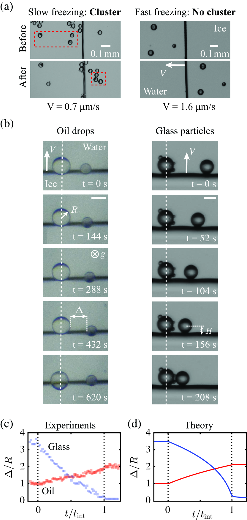
Figure 1: Interactions between two particles at a moving solidification front. (a) Glass particle distribution before and after engulfment into the ice for slow and fast freezing. (b) Sequence of images capturing the relative dynamics of two oil droplets (left) and glass particles (right) at an advancing solidification front in the reference frame of the larger particle. The velocity at which the front propagates is slightly above the critical velocity $V_{\mathrm{crit}}$, that governs particle rejection or engulfment into the solidifying bulk. The scale-bars indicate a length of $50\text{\,}\mathrm{\SIUnitSymbolMicro m}$. (c)-(d) Shortest lateral distance between two particles $\Delta(t)$ as a function of dimensionless time, experimentally (c) and theoretically (d). Oil drops ( ) are observed to repel whereas glass particles ( ) attract.

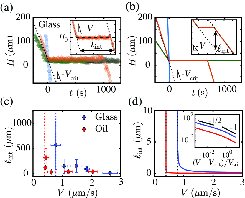
Figure 2: Freezing of a single particle. Front-particle distance $H(t)$ during the freezing of an isolated particle for experiments (a) and theory (b). Depending on the front velocity, three typical scenario are observed: full rejection ( ) at low freezing rate, no displacement ( ) for fast freezing, and partial rejection ( ) at intermediate speed. The insets highlight the definition of the particle-front interaction time $t_{\mathrm{int}}$ and length $\ell_{\mathrm{int}}$. Experimental (c) and theoretical (d) particle-front interaction length as a function of advancing velocity $V$ for single oil drops ( ) and glass particles ( ). The interaction length rapidly increases as $V$ approaches $V_{\mathrm{crit}}$ (dotted lines), where $V_{\mathrm{crit,oil}}\approx$0.39\text{\,}\mathrm{\SIUnitSymbolMicro m}\text{\,}{\mathrm{s}}^{-1}$$ and $V_{\mathrm{crit,glass}}\approx$0.78\text{\,}\mathrm{\SIUnitSymbolMicro m}\text{\,}{\mathrm{s}}^{-1}$$. Only the Hamaker constant $A$ is fitted to match the critical velocity $V_{\mathrm{crit}}$ in the theoretical model. We find $A_{\mathrm{oil}}\sim 10^{-21}$\text{\,}\mathrm{J}$$ and $A_{\mathrm{glass}}\sim 10^{-19}$\text{\,}\mathrm{J}$$. The inset on a log-log scale in (d) highlights the critical behaviour of $\ell_{\mathrm{int}}\propto(V-V_{\mathrm{crit}})^{-1/2}$.

We turn to our theoretical description that extends the models for single particle trapping in ice [30, 27, 28, 29]. The first challenge is to predict the repelling velocity $\mathbf{U}$ of a particle near a solidification front, which must be normal to the solid-liquid interface by symmetry. Particles engulfed in ice are known to be surrounded by a premelted liquid layer coming from intermolecular interactions [31]. We suppose that these interactions are the main cause of the particle repulsion by the moving front, and assume the presence of a van-der-Waals disjoining pressure, as $\Pi(\mathbf{x})=A/(6\pi d^{3}(\mathbf{x}))$, where $A$ is the Hamaker constant and $d(\mathbf{x})$ the local particle-front distance. Hence the repelling force $\mathbf{F}_{\Pi}$ can be found by integrating the disjoining pressure on the particle surface. The moving particle experiences a viscous friction force $\mathbf{F}_{\mathrm{vis}}$ opposing the particle motion, hence effectively attracting the particle towards the ice and promoting particle engulfment. The lubrication approximation is used to compute the friction force (Supp. Mat., Sec. II). The particle repelling velocity is then determined from the force balance $\mathbf{F}_{\Pi}+\mathbf{F}_{\mathrm{vis}}=\mathbf{0}$.

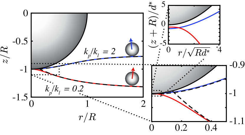
Figure 3: Solid-liquid interface shape. Numerical solution of the solid-liquid interface for $H=R(1+k_{e})$, with a conductivity ratio of $k_{p}/k_{l}=2$, i.e., $k_{e}=-0.25$, (blue, corresponding to glass particles) and $k_{p}/k_{l}=0.2$, i.e., $k_{e}=0.36$, (red, corresponding to oil droplets). A neighbouring particle might interact with the inclined interface, causing them to attract or repel, as shown with the schematic. A thin liquid film of typical thickness $d^{*}$ is separating the particle from the solid-liquid interface, as seen in the top right panel, which is a rescaled zoom-in of the first zoom-in. The dashed black lines correspond to the asymptotic limits away from the particle, that only deviate from the full solution at its base.

The precise shape of the freezing interface is required to compute the forces and is determined through the interface temperature condition. Under standard conditions the solid-liquid interface temperature $T_{i}(\mathbf{x})$ is given by the melting temperature of water $T_{m}$. In close proximity to the particle, however, the equilibrium condition changes due to local variations in pressure that reduce the melting temperature. The interface temperature is then [32]

$$T_{i}(\mathbf{x})=T_{m}-\frac{T_{m}}{\rho_{s}\mathcal{L}}\,\Delta p(\mathbf{x}),\quad\text{with}$$ (1a)

$$\Delta p(\mathbf{x})=\sigma_{\mathrm{sl}}\mathcal{K}(\mathbf{x})+\Pi(\mathbf{x}),$$ (1b)

where $\rho_{s}$ is the mass density of ice, $\mathcal{L}$ the latent heat, $\sigma_{\mathrm{sl}}$ is the surface energy of the solidification front and $\mathcal{K}$ its local curvature. Then, the heat equation allows to get a second condition for the interface. We assume that thermal diffusion dominates over convection , and the temperature field to be steady. Hence, the temperature follows Fourier’s law $\nabla^{2}T=0$ in both phases. An external far-field thermal gradient $\mathbf{G}=G\mathbf{e}_{z}$ is applied, and a spherical particle of radius $R$ is placed at a distance $H$ from the reference undeformed front, where its center of mass is at $\mathbf{x}_{0}$. The thermal conductivity of the particle and the surrounding liquid are denoted by $k_{p}$ and $k_{l}$. For simplicity, the ice is assumed to have the same conductivity as water, i.e., $k_{i}=k_{l}$, whereas in reality $k_{i}/k_{l}=4$. The heat equation can then be solved exactly [30] and the solid-liquid interface corresponds to the isotherm that matches the melting temperature in the far field, which is given by

$$T_{i}(\mathbf{x})=T_{m}+GH+\mathbf{G}\cdot(\mathbf{x}-\mathbf{x}_{0})+k_{e}R^{3}\,\frac{\mathbf{G}\cdot(\mathbf{x}-\mathbf{x}_{0})}{|\mathbf{x}-\mathbf{x}_{0}|^{3}}$$ (2)

with $k_{e}=(k_{l}-k_{p})/(2k_{l}+k_{p})$, with $-1<k_{e}<1/2$, is the dimensionless parameter that quantifies the mismatch in the thermal conductivities. Importantly, when the particle and liquid have different thermal conductivities, $k_{e}\neq 0$, the solid-liquid interface is shifted because of the heat flux boundary condition at the particle surface, leading to the extra term of dipolar symmetry in (2).

Combining equations (1) and (2) yields an expression for the shape of the solidification front, which can be solved numerically for any particle-front distance (Supp. Mat., Sec. III). The shape of the solid-liquid interface is shown in Fig. 3 for both more and less conductive particles when the front-particle distance $H=R(1+k_{e})$. The latter corresponds to the typical distance at which particle and ice nearly touch. A thin liquid film, of typical thickness $d^{*}\sim R[A/(6\pi R^{2}\sigma_{\mathrm{sl}})]^{1/3}$, is separating the particle from the interface. It is set by balancing the disjoining pressure with the Laplace pressure $A/(6\pi d^{*3})\sim\sigma_{\mathrm{sl}}/R$ [28]. For particles less conductive than water, the heat flux is deflected away from the particle, which causes the isotherm to bend toward the particle (blue line in Fig. 3, see also Supp. Mat., Fig. S3 in Sec. IV) and the other way around for more conductive particles (red line in Fig. 3).

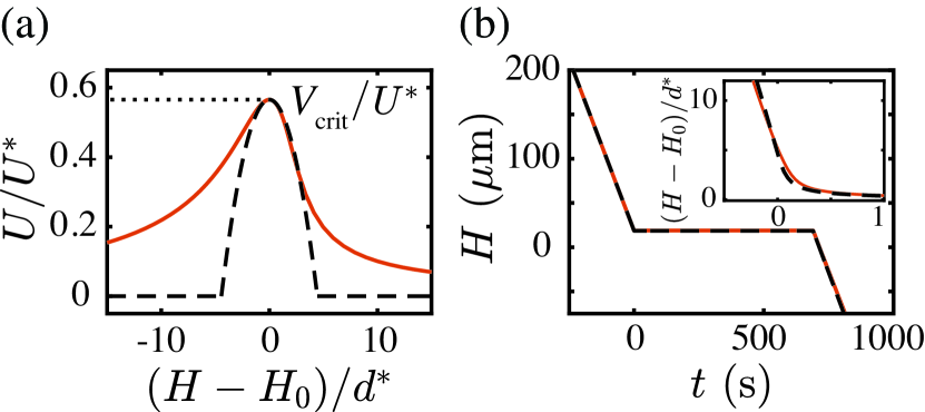
Figure 4: Particle repelling velocity. (a) Theoretical dimensionless particle velocity $U/U^{*}$ as a function of the rescaled particle-front distance $(H-H_{0})/d^{*}$. The critical velocity corresponds to the maximum of the particle velocity. The dashed lines show the approximated velocity used in the simplified theoretical model. (b) Numerical (solid line) and analytical (dashed line) front-particle distance $H(t)$ as function of time. The inset shows a rescaled zoom-in.

Now that the shape of the solid-liquid interface is known, we can compute both the repelling and the friction force and find the particle velocity. At the scaling level, the typical particle velocity $U^{*}$ is obtained by balancing the viscous lubrication pressure $\mu U^{*}R/d^{*2}$ with the disjoining pressure $A/(6\pi d^{*3})$, which gives $U^{*}=A/(6\pi\mu Rd^{*})$. The dimensionless particle velocity resulting from out calculation is plotted in Fig. 4(a) versus the particle-front distance and displays a maximum at a finite distance denoted $H_{0}$. Indeed, at a distance much larger than $H_{0}$, the disjoining pressure is small, so that $U(H\to\infty)\rightarrow 0$. As the particle gets very close to the front, the viscous friction increases, leading to $U(H\to 0)\rightarrow 0$. The maximum velocity corresponds to the critical velocity $V_{\mathrm{crit}}$ as steady stable solutions, where $U=V$ can only be found if the front velocity is smaller than $V_{\mathrm{crit}}$.

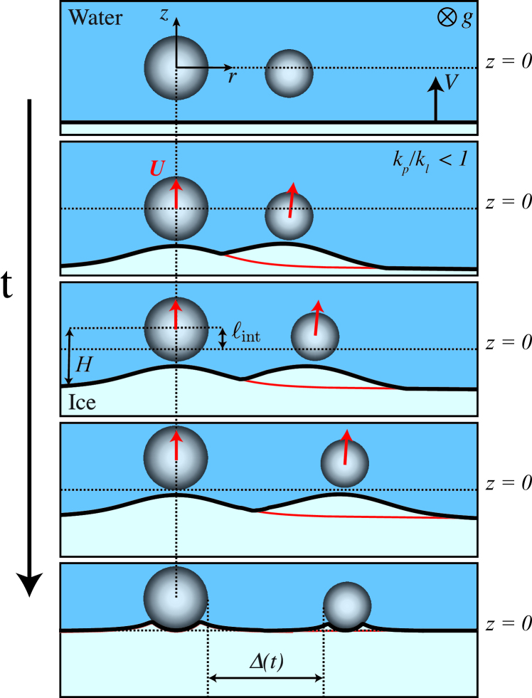
Figure 5: Mechanism of the particle-particle interactions. Schematic representation of the particle-particle interaction at the moving solidification front in the case of particles less conductive than the surrounding liquid, i.e., $k_{e}>0$, i.e., repelling particles. The thin red line indicates the shape of the solid-liquid interface in the absence of the second particle. As the particles interact with the advancing front, they start to move with velocity $\mathbf{U}$, causing a vertical displacement $\ell_{\mathrm{int}}$ during the time of interaction $t_{\mathrm{int}}$, as well as a lateral displacement, represented by $\Delta\,(t)$.

When the front velocity is slightly larger than $V_{\mathrm{crit}}$, say $V=V_{\mathrm{crit}}+\delta V$, the particle spends most of the time close to the front, getting repelled (Fig. 2(b)). Hence, we must characterize this stage of the full dynamics to estimate the particle trajectories. To obtain analytic insights, we simplify the analysis and suppose that the particle velocity is a piecewise defined function (see dashed lines in Fig. 4(a)), that follow the Taylor expansion of $U$ near $H_{0}$ as $U(H)\simeq V_{\mathrm{crit}}-B(H-H_{0})^{2}$ and $U(H)=0$ elsewhere. With this approximation the particle repelling trajectory can be obtained analytically (Supp. Mat., Sec. V), which provides a very good description of the full dynamics for front velocities close to the critical velocity (Fig. 4(b)). In particular, in the limit where $\delta V\ll V$, we find that the interaction time and length follow the asymptotic expressions

$$t_{\mathrm{int}}=\pi B^{-1/2}(V-V_{\mathrm{crit}})^{-1/2},$$ (3a)

$$\ell_{\mathrm{int}}=V_{\mathrm{crit}}\,t_{\mathrm{int}}=\pi V_{\mathrm{crit}}B^{-1/2}(V-V_{\mathrm{crit}})^{-1/2},$$ (3b)

which again agrees quantitatively with the full dynamics (Fig. 2(d)). Such scaling relations resemble the critical exponents found for second-order phase transition models within the mean-field approximation [34]. We did not try to verify the prediction of the critical exponent experimentally because of the intrinsic noise, with front velocity fluctuations being of the order of $\pm 10\%$. Therefore, it is not possible to set the front velocity close to the critical velocity with a good enough accuracy. This inherent variability is also responsible for the notable scatter of the experimental data (Fig. 2(c)), as we approach this critical point and the lack of quantitative agreement between Fig. 2(c) and (d). However, an excellent qualitative agreement is found, where the only adjustable parameter is the Hamaker constant, characterizing the particle-front interactions. For simplicity, we have omitted the effects of water expansion during freezing [35], as well as flows driven by thermo-capillarity [29], that should not qualitatively modify the interaction length criticality (Supp. Mat., Sec. VI), but would certainly change the fitted Hamaker constant. Lastly, in the other limit when the front velocity is much larger than the critical velocity, the interaction length is found to decay asymptotically as $1/V$. More specifically, it scales as $d^{*}V_{\mathrm{crit}}/V$ (Supp. Mat., Sec. V).

We now come back to particle-particle interactions at an advancing solidification front and suppose the presence of a second particle at distance $\Delta$ from the other (Fig. 5). Both particles are getting repelled in the normal direction to the solid-liquid interface. The repulsion mechanism being short-range interactions, we do not expect the presence of a second particle to drastically alter the front-particle dynamics in the normal direction. However, the shape of the solid-liquid interface will result from the sum of the individual front-particle interactions. We suppose that each particle is getting repelled in the normal direction to the local slope generated by the other particle, which causes effective particle-particle interactions. Hence, the tangential velocity is given by $U_{r}=-U_{z}\frac{\partial z}{\partial r}$, where $\frac{\partial z}{\partial r}$ is the local slope at the center of the second particle. This scenario is in agreement with the experimental observation of Fig. 1 that oil droplets repel, while glass particles attract. Indeed, the local slopes of these two cases are opposite (Fig. 3).

Finally, we discuss the shape of the solid-liquid interface at long distance, as it is important to quantify particle-particle interactions. As the particle-front interactions are only significant at short distances (near the base), they do not affect the long-distance solid-liquid interface. Furthermore, the long-range deformation is entirely dictated by the thermal conductivity mismatch, via the dipolar term in (2). In particular, the large-radius limit is found to be asymptotically $z\simeq-H+k_{e}R^{3}H/(H^{2}+r^{2})^{3/2}$, where the cylindrical coordinate system centered on the particle is used (Supp. Mat., Sec. VII). This simplified expression agrees fairly well with the numerical profiles as shown in Fig. 3. The sign of the interface slope changes with $k_{e}$, corresponding to the transition from particles less to more conductive than the surrounding liquid. Integrating the radial velocity with the long-range interface slope expression, we obtain a quantitative agreement with the experimental observation (Fig. 1(d)).

To conclude, in this Letter, we have experimentally and theoretically described how two particles interact at a moving solidification front. The nature of the two-body interaction depends on the relative conductivity of the particle with respect to the surrounding liquid, where more (resp. less) conductive particles attract (resp. repel). The strength of the interaction critically depends on the solidification front velocity. The derived model paves the way towards an understanding of cluster formations during solidification. In this context, extending the present formalism to n-body interactions, adding effects such as solute or volume expansion, or treating freezing suspensions with different types of particles offer a wide range of perspectives.

Supplementary Material

List of supplementary movies

• Movie 1: Freezing of a two nearby oil droplets showing some effective repulsion. The translational stage is moving the sample so that the freezing front appears stationary in the video. The front velocity is $V\approx$0.4\text{\,}\mathrm{\SIUnitSymbolMicro m}\text{\,}{\mathrm{s}}^{-1}$$ and the video is acquired at 0.25 frames/sec and sped up 175 times.

• Movie 2: Freezing of a two nearby glass particles showing some effective attraction. The front velocity is $V\approx$0.7\text{\,}\mathrm{\SIUnitSymbolMicro m}\text{\,}{\mathrm{s}}^{-1}$$ and the video is acquired at 0.25 frames/sec and sped up 120 times.

• Movie 3: Freezing of isolated glass particles for three front velocities highlighting the different scenarios depicted in Fig. 2(a), i.e. no particle displacement, partial rejection and full rejection. The videos are acquired at 0.25 frame/sec and sped up 115, 60 and 70 times, respectively.

I - Schematic of the experimental set-up and general details

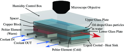
Figure 6: Schematic of the experimental set-up. The arrow indicates the direction in which the Hele-Shaw cell is pushed over the copper block.

In this section we further address some general experimental details and technicalities. A schematic of the experimental set-up is shown in Fig. 6. The exact protocol adopted in our current investigations is as follows. At the beginning of each experiment, the Hele-Shaw cell (Ibidi, $\mu$-Slide I Luer) is placed on a copper block maintained at a fixed thermal gradient and either the oil-in-water emulsion or the glass particles in water suspension is injected. For the bulk we used Milli-Q water. The dispersed phase in the emulsion is silicone oil (Sigma-Aldrich, Germany) with a viscosity of $50\text{\,}\mathrm{c}\mathrm{S}\mathrm{t}$ and the glass microspheres used in the suspension are purchased from Whitehouse Scientific, UK. The emulsion is prepared using an in-house designed co-flow device. To ensure stability a surfactant TWEEN-80 (Sigma-Aldrich, Germany) is added to the water. In the initial phase of our study samples were prepared using different concentrations and dilutions to study the effect the surfactant concentration might have on the observations. For the dilutions that were considered no significant changes were observed. For our current study we have chosen an initial surfactant concentration of $0.5\,\mathrm{vol}\%$, which after diluting the emulsion sample with water was lowered to $0.01\,\mathrm{vol}\%$.

We then initiate the solidification on the colder end of the Hele-Shaw cell by inserting a small piece of ice, that acts as nucleation site. After the initialization, a solidification front forms that slowly advances into the field of view of the camera (Nikon D850 with long working distance lens with a working distance of $86\text{\,}\mathrm{mm}$). If the slide remained stationary, the front would keep advancing until it has propagated out of view. To prevent this from happening and to be able to perform longer experiments, we set the Hele-Shaw cell slide in motion with velocity V, opposite to the direction of motion of the solidification front, using a linear actuator (Physik Instrumente, M-230.25). The lowest velocity that was measured at which the slide can be pushed is $V=$0.1\text{\,}\mathrm{\SIUnitSymbolMicro m}\text{\,}{\mathrm{s}}^{-1}$$. The calibration measurements verified that at this velocity the variations are within 25%. When increasing the velocity the stability increases and the variations fall within 10% for $V\approx$0.4\text{\,}\mathrm{\SIUnitSymbolMicro m}\text{\,}{\mathrm{s}}^{-1}$$ and beyond. By properly choosing V it will appear as if the front remains stationary and that the droplets approach the front, whereas in reality it is vice versa. We therefore change V by changing G. To correct for irregularities in environmental heat losses, that slightly alter the growth rate of the ice, the voltage of the Peltier element on the warmer side is continuously adjusted ($\pm$10\text{\,}\mathrm{mV}$$ roughly every 10 minutes, dependent on whether the front needs to speed up or slow down). We do so to ensure that the solidification front remains stationary in our reference framework. Thus, although V and G can be altered independently, we chose to perform experiments in a manner that the velocity of the freezing front is determined by the applied thermal gradient.

II - Forces acting on the particle

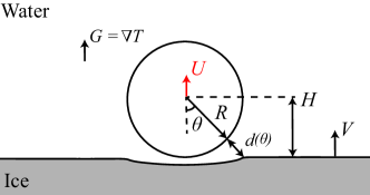
Figure 7: Sketch of the particle-front interaction, where we consider an axisymmetric, spherical coordinate system centered on the particle.

Friction force: viscous lubrication model

As sketched in Fig. 7, we suppose here that a spherical particle is moving away from an advancing solidification front. Following the previous works on the interactions between a particle and a solidification front [27, 28, 29], we use an axisymmetric, spherical coordinate system centered on the particle (see Fig. 7), where $\theta$ is the latitude angle which is defined from the basis of the particle. Although the solid-liquid boundary is translated at a speed $V$, it does not contribute to the friction force, as the liquid particles near the solid-liquid boundary are not moving but freeze. Assuming a no-slip condition, the boundary condition for the velocity field at the solid-liquid surface is $\mathbf{v}=\mathbf{0}$ [36]. On the other hand, the boundary condition for the velocity field at the particle surface is $\mathbf{v}=\mathbf{U}$, where $\mathbf{U}$ is the particle velocity. Due to the combined effect of front-particle intermolecular interactions (see Section III) and heat conduction (see Section IV), the solid-liquid interface is not flat, but curved near the particle. We define the local front-particle distance at a given angle $d(\theta)$ (see Fig. 7). The friction force experienced by the particle depends on the precise shape of the solid-liquid interface.

The intermolecular interactions being short range, the particle repelling velocity is significant only when the particle is very close to the solid-liquid interface. As discussed in the main text, the relevant film thickness at the basis of the particle is $d^{*}\sim R[A/(6\pi R^{2}\sigma_{\mathrm{sl}})]^{1/3}\ll R$, which is much smaller than the particle radius. In this situation, the friction force is largely enhanced as compared to the Stokes drag and can be computed using the viscous lubrication approximation [37]. In this approximation, the viscous pressure only depends on the angle and is uniform in the normal direction to the interface. The viscous pressure follows from the thin-film equation

$$\mathbf{U}\cdot\mathbf{n}=\nabla\cdot\left(\frac{d^{3}}{12\mu}\nabla p_{\mathrm{vis}}\right),$$ (4)

where $\mathbf{n}$ is the normal vector to the interface at a given angle, and $p_{\mathrm{vis}}$ the viscous pressure. Using the spherical coordinate system, this yields

$$U\cos\theta=\frac{1}{R^{2}\sin\theta}\frac{\partial}{\partial\theta}\left(\sin\theta\frac{d^{3}(\theta)}{12\mu}\frac{\partial p_{\mathrm{vis}}(\theta)}{\partial\theta}\right),$$ (5)

where we recall that $d$ and $p_{\mathrm{vis}}$ only depend on the latitude angle. The latter equation can be integrated from the pole $\theta=0$ (the basis of the particle) to an arbitrary latitude $\theta$ to give

$$\frac{\partial p_{\mathrm{vis}}(\theta)}{\partial\theta}=6\mu UR^{2}\frac{\sin\theta}{d^{3}(\theta)}.$$ (6)

The viscous pressure vanishes at large distances, i.e. in the $\theta\rightarrow\pi/2$ limit, so that the equation (6) can further be integrated over $\theta$ to obtain the viscous pressure field as

$$p_{\mathrm{vis}}(\theta)=6\mu UR^{2}\int_{\theta}^{\pi/2}\frac{\sin\hat{\theta}}{d^{3}(\hat{\theta})}\mathrm{d}\hat{\theta},$$ (7)

where the integration constant (reference pressure) is set to zero. Finally, the friction force in the viscous lubrication theory is given by the integral of the viscous pressure on the surface, as

$$\begin{split}F_{\mathrm{vis}}(\theta)&=2\pi R^{2}\int_{0}^{\pi/2}p_{\mathrm{vis}}(\theta)\cos\theta\sin\theta\,\mathrm{d}\theta\\ &=6\pi\mu UR^{4}\int_{0}^{\pi/2}\mathrm{d}\theta\sin 2\theta\int_{\theta}^{\pi/2}\frac{\sin\hat{\theta}}{d^{3}(\hat{\theta})}\,\mathrm{d}\hat{\theta},\end{split}$$ (8)

where we recover the expression as in Ref. [29].

Repelling force

The repelling force, arising from the intermolecular interaction, is similarly obtained by integrating the disjoining pressure $\Pi(\theta)=A/(6\pi d^{3}(\theta))$ over the surface of the particle, as

$$F_{\Pi}(\theta)=2\pi R^{2}\int_{0}^{\pi/2}\Pi(\theta)\cos\theta\sin\theta\,\mathrm{d}\theta=\frac{AR^{2}}{6}\int_{0}^{\pi/2}\frac{\sin 2\theta}{d^{3}(\theta)}\mathrm{d}\theta.$$ (9)

Combining equations (8) and (9) gives rise to a velocity scale

$$\mathcal{W}=A/\mu R^{2}$$ (10)

that is related to the typical particle velocity mentioned in the main text as $U^{*}=\mathcal{W}R/d^{*}$.

III - Numerical calculation of the front interface and particle velocity

As mentioned in the main text, the shape of the solid-liquid interface is obtained by combining the equilibrium condition (also Gibbs-Thompson, see (1)) and the isotherm matching the melting temperature in the far field (see (2)). More specifically, the solid-liquid interface shape follows [27, 28, 29]

$$\frac{T_{m}}{\rho_{s}\mathcal{L}}\,\left[\sigma_{\mathrm{sl}}\mathcal{K}(\mathbf{x})+\Pi(\mathbf{x})\right]+GH+\mathbf{G}\cdot(\mathbf{x}-\mathbf{x}_{0})+k_{e}R^{3}\,\frac{\mathbf{G}\cdot(\mathbf{x}-\mathbf{x}_{0})}{|\mathbf{x}-\mathbf{x}_{0}|^{3}}=0.$$ (11)

We again use the spherical coordinate system centered on the particle, see Fig. 7, such that the shape of the solid-liquid interface is determined via the local particle-front distance $d(\theta)$ as

$$L_{\sigma}\mathcal{K}R+\frac{L_{\Pi}^{4}}{d^{3}(\theta)}=(R+d(\theta))\cos\theta\left[1+k_{e}\left(\frac{R}{R+d(\theta)}\right)^{3}\right]-H,$$ (12)

where we introduce the length scales as in Refs. [27, 28, 29]

$$L_{\sigma} =\frac{T_{m}\sigma_{\mathrm{sl}}}{\rho_{s}\mathcal{L}GR}, L_{\mathrm{\Pi}} =\left(\frac{AT_{m}}{6\pi\rho_{s}\mathcal{L}G}\right)^{1/4}.$$ (13)

The typical film thickness near the basis of the particle $d^{*}$ can be found balancing the disjoining pressure with the Laplace pressure as $A/(6\pi d^{*3})\sim\sigma_{\mathrm{sl}}/R$, which is also related to the aforementioned lengths scales via $d^{*}=\left(L_{\Pi}^{4}/L_{\sigma}\right)^{1/3}=R[A/(6\pi R^{2}\sigma_{\mathrm{sl}})]^{1/3}$. Defining the solid-liquid interface with the front-particle distance $d$, the curvature of the latter follows as

$$\mathcal{K}=\left[\frac{-2(R+d)^{2}+(R+d)d^{\prime\prime}-3d^{\prime 2}}{((R+d)^{2}+d^{\prime 2})^{3/2}}+\frac{\cos\theta}{\sin\theta}\frac{d^{\prime}}{(R+d)((R+d)^{2}+d^{\prime 2})^{1/2}}\right],$$ (14)

with primes denoting derivatives with respect to $\theta$.

Non-dimensionalization

We rescale all the lengths in (12) by the radius of the particle $R$ so the dimensionless interface equation becomes

$$l_{\sigma}\kappa+\frac{l_{\Pi}^{4}}{\delta^{3}(\theta)}=(1+\delta)\cos(\theta)\left[1+k_{e}\left(\frac{1}{1+\delta(\theta)}\right)^{3}\right]-h,$$ (15)

where the rescaled variables are given by

$$\delta(\theta)=d(\theta)/R,\quad\quad h=H/R,\quad\quad l_{\sigma}=L_{\sigma}/R\quad\text{and}\quad l_{\Pi}=L_{\Pi}/R.$$ (16)

The dimensionless curvature $\kappa$ follows

$$\kappa=\frac{-2(1+\delta)^{2}+(1+\delta)\delta^{\prime\prime}-3\delta^{\prime 2}}{((1+\delta)^{2}+\delta^{\prime 2})^{3/2}}+\frac{\cos\theta}{\sin\theta}\frac{\delta^{\prime}}{(1+\delta)((1+\delta)^{2}+\delta^{\prime 2})^{1/2}},$$ (17)

with primes again denoting derivatives with respect to $\theta$.

Dynamics

We have assumed that both the fluid transport (Stokes flow), and the heat transport are steady. Hence, equation (15) holds for any instant $t$. We wish to determine the dynamics of the particle during the freezing. Therefore, we introduce time and set the initial particle position far from the front, typically $H(t=0)=1.5(R+k_{e})$. Hence, $d$, $H$ and $U$ are now time-dependent. The variation of particle-front distance is given by

$$\frac{\mathrm{d}h}{\mathrm{d}t}=u(t)-v,$$ (18)

where $u(t)=U(t)/\mathcal{W}$ and $v=V/\mathcal{W}$ are the dimensionless velocities and the time is nondimensionalized using $R/\mathcal{W}$ as a time scale. The particle velocity is set by the force balance $F_{\Pi}+F_{\mathrm{vis}}=0$. Injecting (8) and (9), and using dimensionless variables, we find

$$u(t)\int_{0}^{\pi/2}\mathrm{d}\theta\sin 2\theta\int_{\theta}^{\pi/2}\frac{\sin\hat{\theta}}{\delta^{3}(\hat{\theta},t)}\,\mathrm{d}\hat{\theta}+\int_{0}^{\pi/2}\frac{\sin 2\theta}{\delta^{3}(\theta,t)}\mathrm{d}\theta=0.$$ (19)

Numerical discretization

We now provide the numerical scheme that has been used to find the particle-front dynamics in Fig. 2(b) of the main text. Let us introduce a homogeneously discretized angular axis $\theta_{i}=i\mathrm{d}\theta$ on the interval $[0,\theta_{c}]$, where $\theta_{c}=N\mathrm{d}\theta=\pi/2$, with $N$ the number of angular grid points. In addition, we discretize time as $(t)^{n}=n\mathrm{d}t$, where superscript is used for the time discretization. The discretization of (15) is

$$l_{\sigma}(\kappa)_{i}^{n}+\frac{l_{\Pi}^{4}}{\left(\delta^{3}\right)_{i}^{n}}=(1+(\delta)_{i}^{n})\cos\theta_{i}\left[1+k_{e}\left(\frac{1}{1+(\delta)_{i}^{n}}\right)^{3}\right]-(h)^{n},$$ (20)

where the discrete curvature (see (17)) is given by

$$(\kappa)_{i}^{n}=\frac{-2(1+(\delta)_{i}^{n})^{2}+(1+(\delta)_{i}^{n})\left(\delta^{\prime\prime}\right)_{i}^{n}-3\left(\delta^{\prime 2}\right)_{i}^{n}}{((1+(\delta)_{i}^{n})^{2}+\left(\delta^{\prime 2}\right)_{i}^{n})^{3/2}}+\frac{\cos\theta_{i}}{\sin\theta_{i}}\frac{\left(\delta^{\prime}\right)_{i}^{n}}{(1+(\delta)_{i}^{n})((1+(\delta)_{i}^{n})^{2}+\left(\delta^{\prime 2}\right)_{i}^{n})^{1/2}}.$$ (21)

The angular derivative are discretized by using the following finite-difference scheme

$$\left(\delta^{\prime\prime}\right)_{i}^{n} =\frac{(\delta)_{i+1}^{n}-2(\delta)_{i}^{n}+(\delta)_{i-1}^{n}}{\mathrm{d}\theta^{2}}, \left(\delta^{\prime}\right)_{i}^{n} =\frac{(\delta)_{i+1}^{n}-(\delta)_{i}^{n}}{\mathrm{d}\theta}.$$ (22)

The front-particle dynamical equation is discretized by using an explicit scheme

$$(h)^{n+1}-(h)^{n}=((u)^{n}-v)\mathrm{d}t,$$ (23)

where the particle velocity is given by

$$(u)^{n}\sum_{i=1}^{N}\mathrm{d}\theta\sin 2\theta_{i}\sum_{j=i}^{N}\frac{\sin\theta_{N-j}}{\left(\delta^{3}\right)_{N-j}^{n}}\mathrm{d}\theta+\sum_{i=1}^{N}\frac{\sin 2\theta_{i}}{\left(\delta^{3}\right)_{i}^{n}}\mathrm{d}\theta=0.$$ (24)

We impose the following boundary conditions on the local particle-interface distance, that are

$$\delta^{\prime}(\theta=0)=0\quad\rightarrow\quad(\delta)_{2}^{n}-(\delta)_{1}^{n}=0,$$ (25)

$$\delta(\theta=\theta_{c})=\frac{h}{\cos\theta_{c}}-1\quad\rightarrow\quad(\delta)_{N}^{n}=\frac{(h)^{n}}{\cos\theta_{N}}-1,$$ (26)

that correspond to the symmetry condition at the center and we assume an undeformed, planar interface of the solidification front far from the center.

Assuming that $(\delta_{i})^{n}$ and $(h)^{n}$ are known, the algorithm performs the following steps. First, we determine the new particle-front distance $(h)^{n+1}$ by using (23) and (24). Then, we find the new local front-particle distance solving the non-linear equation (20), using an optimised root-finding algorithm. The numerical code used in this article is available at .

IV - Qualitative interpretation of the front deflection due to conductivity mismatch

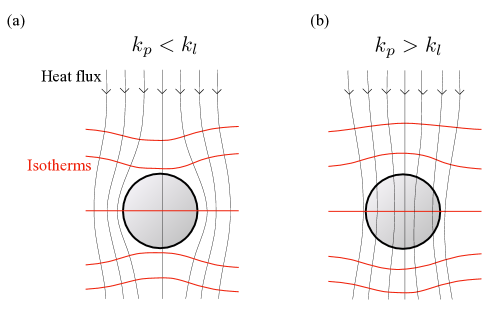
Figure 8: Schematic of the heat flux streamlines and isotherms when a particle is placed in an uniform external temperature gradient. In (a) (resp. (b)), the particle is less (resp. more) conductive than the surrounding liquid.

We provide here a qualitative explanation about the effects of the thermal conductivity mismatch on the solid-liquid interface observed in the Fig. 3 of the main text. We consider a system with a uniform external temperature gradient. Hence, the heat flux streamlines are straight and in the direction of the temperature gradient, via Fourier’s law. When a particle of different thermal conductivity is placed in the system, the heat flux streamlines will bend in the vicinity of the particle. If the particle is less conductive, the heat flux will be deflected away from the particle as the resistance is higher at the particle (see (a) in Fig. 8). The isotherms being orthogonal to the heat flux, they bend towards the particle. The opposite occurs for more conductive particles, such that the isotherms bend away from the particles. The solid-liquid interface being an isotherm at the melting temperature, we observe similar front deflections as the one depicted in Fig. 8.

V - Particle-front interaction length

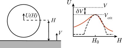
Figure 9: Sketch of the particle repelling velocity as a function of front-particle distance $H$. The red solid line shows the full solution, the black dashed line the parabolic approximation.

We wish to determine the distance travelled by the particle before getting engulfed, denoted $\ell_{\mathrm{int}}$ (see Fig. 2 of the main text). The latter can be computed by integrating the particle velocity in time as

$$\ell_{\mathrm{int}}=\int_{0}^{\infty}U[H(t)]\,\mathrm{d}t.$$ (27)

In the steady framework derived here, the particle velocity does not depend explicitly on time and is a function of the particle front distance $H(t)$ only. For very large particle-front distance, the intermolecular forces are negligible, so that the repelling force goes to zero, so does $U$. On the other hand, as $H$ decreases, the friction force increases so that the particle velocity also goes to zero in the limit $H\to-\infty$. Hence, $U(H)$ has a maximum at a given front-particle distance $H_{0}$, as drawn schematically in Fig. 9 (see also Fig. 4 of the main text for an example of numerical curve). The particle velocity at the maximum $U(H_{0})$ correspond to the critical engulfment velocity $V_{\mathrm{crit}}$. Indeed, if $V<V_{\mathrm{crit}}$, steady dynamical solutions can be found where the particle is indefinitely repelled. Therefore, the particle-front interaction length is only defined when $V>V_{\mathrm{crit}}$. We stress that once the particles and fluid properties are fixed, $\ell_{\mathrm{int}}$ only depends on the solidification front velocity $V$. The goal of this section is to describe the asymptotic behavior of the interaction length in both limits $V\rightarrow V_{\mathrm{crit}}^{+}$ and $V\gg V_{\mathrm{crit}}$.

Critical behavior near the engulfment velocity

We define the deviation of the front velocity with respect to the critical speed as $\delta V=V-V_{\mathrm{crit}}$. We are interested here in the limit where $\delta V\ll V_{\mathrm{crit}}$, which means for front velocities approaching the critical velocity. This regime corresponds to the situation where the particle is dragged by the front for a certain time before getting engulfed (see red dots in Fig. 2 of the main text). In this case, the typical time derivative of the particle-front distance is much smaller than the front velocity, i.e. $\frac{\mathrm{d}H}{\mathrm{d}t}=U-V\sim\delta V\ll V$ when the particle is near $H\simeq H_{0}$. The challenge is to obtain the time the particle spends in this region before getting engulfed.

To get analytical insight, we approximate the full $U(H)$ curve with a simpler function. To recover the asymptotic behavior when $\delta V\ll V_{\mathrm{crit}}$, the approximate function should correctly describe $U(H)$ in the vicinity of $H_{0}$. Hence, we choose a piecewise-defined function $U_{0}(H)$ (black dashed line in Fig. 9) that corresponds to the second order Taylor expansion of the full $U(H)$ curve near $H=H_{0}$, truncated such that $U_{0}$ is non negative. Specifically, $U_{0}$ is defined as

$$\begin{split}U(H)&\approx U_{0}(H)=V_{\mathrm{crit}}-B(H-H_{0})^{2},\\ &\text{for }\rvert H-H_{0}\rvert<\Delta H=\sqrt{\frac{V_{\mathrm{crit}}}{B}},\end{split}$$ (28)

where $B=-2U^{\prime\prime}(H)|_{H=H_{0}}$ is a positive constant that can be found numerically. With this approximation, the time evolution of the front-particle distance follows

$$\frac{\mathrm{d}H}{\mathrm{d}t}\simeq U_{0}-V=-\delta V-B(H-H_{0})^{2},$$ (29)

which can now be integrated analytically. The reference time $t=0$ is set at the moment where particle and front start interacting, leading to the initial condition $H(0)=H_{0}+\Delta H$. The equation (29) can be integrated analytically such that the particle-front distance follows

$$H(t)=H_{0}-\delta V\tau\tan\left(\frac{t}{\tau}-\phi\right),\quad\quad\tau=\sqrt{\frac{1}{B\delta V}},$$ (30)

where we identify a typical time scale $\tau$. The integration constant $\phi$ is found by using the initial condition, which leads to

$$\phi=\arctan\left(\frac{V_{\mathrm{crit}}}{\delta V}\right).$$ (31)

The time $t_{\mathrm{int}}$ at which the interaction stops in this simplified model is when $H(t_{\mathrm{int}})=H_{0}-\Delta H$, which leads to

$$t_{\mathrm{int}}=2\phi\tau\simeq\pi\tau,$$ (32)

where the approximation in equation (32) corresponds to the $\delta V\ll V_{\mathrm{crit}}$ limit. Lastly, the interaction length, or the distance travel by the particle can be found using (27), which leads to

$$\ell_{\mathrm{int}}=V_{\mathrm{crit}}t_{\mathrm{int}},$$ (33)

to leading order in the limit $\delta V\ll V_{\mathrm{crit}}$. Equation (33) corresponds to (3) of the main text.

Asymptotic solution at large front velocity

In the fast-freezing limit where $V\gg V_{\mathrm{crit}}$, the particle velocity is always much smaller than the front velocity as $U$ is bounded by $V_{\mathrm{crit}}$. Hence, the particle-front distance rate of change can be approximated by $\frac{\mathrm{d}H}{\mathrm{d}t}=U-V\approx-V$. Hence, the particle-front distance is approximately $H(t)\simeq H_{i}-Vt$, where $H_{i}$ is the initial condition. Therefore, the interaction length can be estimated by performing the following change of variable

$$\ell_{\mathrm{int}}=\int_{0}^{\infty}U(t)\,\mathrm{d}t=\frac{1}{V}\,\int_{-\infty}^{\infty}U(H)\,\mathrm{d}H.$$ (34)

The typical scale of the particle velocity and its $H$ variations are $V_{\mathrm{crit}}$ and $d^{*}$, respectively. Therefore, the typical scaling relationship of the interaction length at large front velocity is $\ell_{\mathrm{int}}\sim d^{*}V_{\mathrm{crit}}/V$, as stated in the main text.

VI - Water expansion and thermo-capillary effects

In the current analysis, we omitted the effects of water expansion during freezing, as well as flow driven by thermo-capillarity in the case of drops, i.e., the thermocapillary migration due to the Marangoni force [39, 40, 17]. When taken these effects into account, they will alter the particle force balance and therefore the particle repelling velocity (see Fig. 4 of the main text). More specifically, one would need to include two additional forces, $\mathbf{F}_{\mathrm{vol}}$ and $\mathbf{F}_{\mathrm{Ma}}$, that correspond to these effects, respectively. These additional force contributions have been derived in the Ref. [29] in the same coordinate system as in Fig. 7, and read

$$F_{\mathrm{vol}}(\theta)\sim-\pi\mu R^{2}V\rho^{\prime}\int_{0}^{\pi/2}\mathrm{d}\theta\sin 2\theta\int_{\theta}^{\pi/2}\frac{[R+d^{2}(\hat{\theta})]\sin\hat{\theta}}{d^{3}(\hat{\theta})}\mathrm{d}\hat{\theta},$$ (35)

where $V$ is the advancing velocity of the solid-liquid interface and $\rho^{\prime}=1-\rho_{s}/\rho_{l}$ quantifies the change in density between the solid (ice) and liquid (water). For the thermo-capillary effects we have the Marangoni force as

$$F_{\mathrm{Ma}}(\theta)\sim\pi R^{2}\frac{\partial\sigma}{\partial T}\int_{0}^{\pi/2}\mathrm{d}\theta\sin 2\theta\int_{\theta}^{\pi/2}\frac{1}{d(\hat{\theta})}\frac{\partial T}{\partial\hat{\theta}}\mathrm{d\hat{\theta}},$$ (36)

with $\partial\sigma/\partial T$ is the thermal coefficient of the interfacial surface tension between the droplet and the surrounding liquid. We decide to ignore these effects for the sake of clarity and simplicity. We anticipate that the addition of such effects would modify the precise form of the $U(H)$ function. However, the critical behavior of the interaction length for $V\simeq V_{\mathrm{crit}}$, extensively discussed in the previous section, will remain unaltered, up to a change in the prefactor $B$.

VII - Shape of the solid-liquid interface at large distance

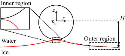
Figure 10: Sketch of the shape of the solid-liquid interface (red line). The solution to the inner region is governed by intermolecular interactions, whereas the outer region is given by the solution governed by the thermal conductivity mismatch (black-dashed line).

The solid-liquid interface profile is mainly governed by the thermal conductivity mismatch at large distances, see outer region in Fig. 10. Indeed, far from the base of the sphere, the short-range disjoining pressure, governing the solution of the inner region, can be neglected and the interface position follows

$$\frac{T_{m}\sigma_{\mathrm{sl}}}{\rho_{s}\mathcal{L}}\mathcal{K}(\mathbf{x})+GH+\mathbf{G}\cdot(\mathbf{x}-\mathbf{x}_{0})+k_{e}R^{3}\,\frac{\mathbf{G}\cdot(\mathbf{x}-\mathbf{x}_{0})}{|\mathbf{x}-\mathbf{x}_{0}|^{3}}=0,$$ (37)

where $\mathcal{K}(\mathbf{x})$ is the local curvature of the solid-liquid interface. Equation (37) compares the solid-liquid Laplace pressure to the thermal gradient, which has the same form as the hydrostatic pressure. Therefore, a length scale arises comparing these two pressures that is analogous to the capillary length in a gravito-capillary system, as

$$\sqrt{\frac{T_{m}\sigma_{\mathrm{sl}}}{\rho_{s}\mathcal{L}G}}=\sqrt{L_{\sigma}R}$$ (38)

For water-ice, with a thermal gradient $G=$10\text{\,}\mathrm{K}\text{\,}{\mathrm{cm}}^{-1}$$ and surface energy $\sigma_{\mathrm{sl}}=$0.03\text{\,}\mathrm{J}\text{\,}{\mathrm{m}}^{-2}$$ [27], the thermal capillary length is of the order of $1\text{\,}\mathrm{\SIUnitSymbolMicro m}$, and is much smaller than the particle radii in our experiments. Therefore, capillary effects are not predominant here at large distances, as the typical curvature of the interface is $1/R\ll 1/\sqrt{L_{\sigma}R}$. As a result, the capillary term can be neglected as well, and equation (37), written in cylindrical coordinates reads

$$H+z+k_{e}R^{3}\frac{z}{(z^{2}+r^{2})^{3/2}}=0.$$ (39)

Lastly, performing a expansion around the flat melting interface as $z=-H+\delta z$, with $\delta z\ll H$, we find

$$z\simeq-H+k_{e}R^{3}H/(H^{2}+r^{2})^{3/2},$$ (40)

which corresponds to the result stated in the main text (dashed lines in Fig. 3).

References

- Deville [2017] S. Deville, Freezing colloids: observations, principles, control, and use: applications in materials science, life science, earth science, food science, and engineering (Springer, 2017).
- Amit et al. [2017] S. K. Amit, M. M. Uddin, R. Rahman, S. Islam, and M. S. Khan, A review on mechanisms and commercial aspects of food preservation and processing, Agriculture & Food Security 6, 1 (2017).
- Rempel [2010] A. W. Rempel, Frost heave, Journal of Glaciology 56, 1122 (2010).
- Peppin et al. [2011] S. Peppin, A. Majumdar, R. Style, and G. Sander, Frost heave in colloidal soils, SIAM Journal on Applied Mathematics 71, 1717 (2011).
- Peppin and Style [2013] S. S. Peppin and R. W. Style, The physics of frost heave and ice-lens growth, Vadose Zone Journal 12 (2013).
- Bronstein et al. [1981] V. Bronstein, Y. Itkin, and G. Ishkov, Rejection and capture of cells by ice crystals on freezing aqueous solutions, Journal of Crystal Growth 52, 345 (1981).
- Körber [1988] C. Körber, Phenomena at the advancing ice–liquid interface: solutes, particles and biological cells, Quarterly Reviews of Biophysics 21, 229 (1988).
- Muldrew et al. [2004] K. Muldrew, J. P. Acker, J. A. Elliott, and L. E. McGann, The water to ice transition: implications for living cells, in Life in the frozen state (CRC Press, 2004) pp. 93–134.
- Gerber et al. [2022] D. Gerber, L. A. Wilen, F. Poydenot, E. R. Dufresne, and R. W. Style, Stress accumulation by confined ice in a temperature gradient, Proceedings of the National Academy of Sciences 119, e2200748119 (2022).
- Carte [1961] A. Carte, Air bubbles in ice, Proceedings of the Physical Society 77, 757 (1961).
- MAENO [1967] N. MAENO, Air bubble formation in ice crystals, Physics of Snow and Ice: proceedings 1, 207 (1967).
- Bari and Hallett [1974] S. Bari and J. Hallett, Nucleation and growth of bubbles at an ice–water interface, Journal of Glaciology 13, 489 (1974).
- Wei et al. [2000] P. Wei, Y. Kuo, S. Chiu, and C. Ho, Shape of a pore trapped in solid during solidification, International Journal of Heat and Mass Transfer 43, 263 (2000).
- Wei and Ho [2002] P. Wei and C. Ho, An analytical self-consistent determination of a bubble with a deformed cap trapped in solid during solidification, Metallurgical and Materials Transactions B 33, 91 (2002).
- Wei et al. [2004] P. Wei, C. Huang, Z. Wang, K. Chen, and C. Lin, Growths of bubble/pore sizes in solid during solidification—an in situ measurement and analysis, Journal of Crystal Growth 270, 662 (2004).
- Tyagi et al. [2022] S. Tyagi, C. Monteux, and S. Deville, Solute effects on the dynamics and deformation of emulsion droplets during freezing, Soft Matter 18, 4178 (2022).
- Meijer et al. [2023] J. G. Meijer, P. Kant, D. Van Buuren, and D. Lohse, Thin-film-mediated deformation of droplet during cryopreservation, Physical Review Letters 130, 214002 (2023).
- Körber et al. [1985] C. Körber, G. Rau, M. Cosman, and E. Cravalho, Interaction of particles and a moving ice-liquid interface, Journal of Crystal Growth 72, 649 (1985).
- Lipp and Körber [1993] G. Lipp and C. Körber, On the engulfment of spherical particles by a moving ice-liquid interface, Journal of Crystal Growth 130, 475 (1993).
- Saint-Michel et al. [2017] B. Saint-Michel, M. Georgelin, S. Deville, and A. Pocheau, Interaction of multiple particles with a solidification front: From compacted particle layer to particle trapping, Langmuir 33, 5617 (2017).
- Tyagi et al. [2021] S. Tyagi, C. Monteux, and S. Deville, Multiple objects interacting with a solidification front, Scientific Reports 11, 3513 (2021).
- Deville [2008] S. Deville, Freeze-casting of porous ceramics: a review of current achievements and issues, Advanced Engineering Materials 10, 155 (2008).
- Deville et al. [2022] S. Deville, A. P. Tomsia, and S. Meille, Complex composites built through freezing, Accounts of Chemical Research 55, 1492 (2022).
- Sexton et al. [2017] M. Sexton, M. E. Madden, A. L. Swindle, V. Hamilton, B. Bickmore, and A. E. Madden, Considering the formation of hematite spherules on mars by freezing aqueous hematite nanoparticle suspensions, Icarus 286, 202 (2017).
- Dedovets et al. [2018] D. Dedovets, C. Monteux, and S. Deville, Five-dimensional imaging of freezing emulsions with solute effects, Science 360, 303 (2018).
- Vella and Mahadevan [2005] D. Vella and L. Mahadevan, The “cheerios effect”, American Journal of Physics 73, 817 (2005).
- Rempel and Worster [1999] A. Rempel and M. Worster, The interaction between a particle and an advancing solidification front, Journal of Crystal Growth 205, 427 (1999).
- Rempel and Worster [2001] A. Rempel and M. Worster, Particle trapping at an advancing solidification front with interfacial-curvature effects, Journal of Crystal Growth 223, 420 (2001).
- Park et al. [2006] M. S. Park, A. A. Golovin, and S. H. Davis, The encapsulation of particles and bubbles by an advancing solidification front, Journal of Fluid Mechanics 560, 415 (2006).
- Shangguan et al. [1992] D. Shangguan, S. Ahuja, and D. Stefanescu, An analytical model for the interaction between an insoluble particle and an advancing solid/liquid interface, Metallurgical Transactions A 23, 669 (1992).
- Wettlaufer and Worster [2006] J. Wettlaufer and M. G. Worster, Premelting dynamics, Annu. Rev. Fluid Mech. 38, 427 (2006).
- Perez [2005] M. Perez, Gibbs–thomson effects in phase transformations, Scripta Materialia 52, 709 (2005).
- Note [1] The Peclet number is , with typical values for velocity , particle size and thermal diffusivity .
- Chaikin et al. [1995] P. M. Chaikin, T. C. Lubensky, and T. A. Witten, Principles of condensed matter physics, Vol. 10 (Cambridge university press Cambridge, 1995).
- Kao et al. [2009] J. C. Kao, A. A. Golovin, and S. H. Davis, Particle capture in binary solidification, Journal of Fluid Mechanics 625, 299 (2009).
- Davis [2001] S. H. Davis, Theory of solidification (Cambridge University Press, 2001).
- Batchelor [1967] G. K. Batchelor, An introduction to fluid dynamics (Cambridge university press, 1967).
- Note [2] The numerical code can be found at https://github.com/vincent-bertin/frozen_cheerios.
- Young et al. [1959] N. Young, J. S. Goldstein, and M. Block, The motion of bubbles in a vertical temperature gradient, Journal of Fluid Mechanics 6, 350 (1959).
- Subramanian [1983] R. S. Subramanian, Thermocapillary migration of bubbles and droplets, Advances in Space Research 3, 145 (1983).