Carbon Dioxide Emission Minimized Virtual Machine (VM) Placement in Cloud-Fog Network Architecture

Abstract

Cloud computing has provided economies of scale, savings, and efficiency for both individual consumers and enterprises. Its key advantage is its ability to handle increasing amounts of data and provide functionality that gives users the ability to scale their computing resources, including processing, data storage, and networking capabilities. Virtual Machines (VM), enabled via virtualization technology, allow cloud service providers to deliver their services to users. This, however, results in increasing carbon dioxide emissions from increased energy use.

This paper introduces a Mixed-Integer Linear Programming (MILP) model that investigates the VM placement, focusing on the British Telecom (BT) network topology, in a cloud-fog network architecture when renewable energy sources are introduced in the fog layer located near traffic-producing sources. VMs can be placed on nodes hosted on the core, metro, and access (fog) layers. We first investigate the effect of varying traffic on IP over WDM power consumption in the backbone network and the number of optical carrier signals to serve the traffic over a period of time. We later extend the model to consider the CO2-minimized optimal virtual machine placement given the sporadic traffic quantity, and the consideration of solar renewable energy sources placed in data centers located in the access (fog) layer throughout the day, imposed on the VM and the minimum workload requirement of the VM to maintain a service-level agreement (SLA).

This paper suggests a direct proportionality between power consumption and the imposed traffic. When integrating solar power into data centers within the British Telecom (BT) network topology, there was a noticeable reduction in power consumption, amounting to up to 16 percent in nodes that received solar energy. This paper demonstrates that a diminishing VM workload led to decreased VM replication in the metro and access layers for constant profiles. The linear profile exhibited the inverse behavior.

I Introduction

The primary selling point of cloud computing is its ability to accommodate exponential growth in voluminous data and provide entities to host functions by providing access, seemingly boundless, to a continuum of computing resources such as processing, data storage, and networking functions. The virtualization process, utilized by cloud service providers, produces VM services that allow for such functionality [1]. With the ever-increasing demand for cloud computing, strain has been imposed on cloud data centers and the energy utilized from the equipment needed to maintain the computing equipment is increasing. CO2 emissions are directly correlated to the electricity demand, which is expected to increase by 15-30% in 2025 [2].

As an attempt to alleviate the exponentially increasing energy expenditure and the strain imposed on data centers brought by traffic, fog computing is a paradigm that makes available computing components, that are able to host virtual machines, placed closer to traffic producing sources. The fog layer brings forth functionality such as filtering, in which voluminous traffic can be filtered in the fog layer without having redundant data be sent to the cloud layer, thus providing transport network energy and bandwidth savings [3]. Fog computing, in this paper, indicates the data centers located nearby traffic producing sources in the access network.

II Related Work and Background

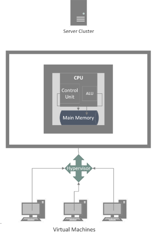
Figure 1: Multiple VM placement on a single server cluster node

Numerous studies have been conducted to further optimize energy usage in the fog layer. In [4], the authors proposed a Green-Demand Aware Fog Computing (GDAFC) solution that uses a prediction technique to map fog server nodes to different work profiles: working nodes, standby nodes, and idle nodes. A prediction model which predicts future volume of requests based on previous trends allocates working nodes for the precedented in, allowing nodes that are not utilized to be placed in idle mode. This resulted in up to 65% savings in energy in the fog layer. In [5], the authors investigate a Lyapunov optimization technique, that derives a greedy algorithm and a joint algorithm, which maps requests, in a network queue, to the amount of energy required to fulfill the requests and investigates whether to dispatch requests one by one or all at once. In [6], the authors investigated the energy efficiency of three different packet routing based objective functions, Objective Function Zero (OF0), Advanced Objective Function Zero (AF0), and Minimum Rank with Hysteresis Objective Function (MRHOF) for Routing Protocol for Low Power and Lossy Networks (RPL) in the fog layer. RPL is a routing protocol that assigns nodes a rank in respect to the root node. OF0 and MRHOF formulate a route based on hop count and expected transmission count respectively. The authors proposed AF0, which routes based on congestion, is optimal for QoS and energy efficiency. It is worth noting that fog computing was not introduced solely for its potential to save power, but to provide users with increased quality of service and low latency by offloading services on fog nodes whenever appropriate.

Cloud computing provides services that are in the form of Infrastructure-as-a-Service (IaaS) [7], allowing users access to processors, routers, and data storage through means of virtualization techniques that allow for data replication, log access, and machinery health. Platform-as-a-Service (PaaS) [7] provides users with an operating system, development tools, and business analytics, that can be accessed through manufacturer-specific API calls. Software-as-a-Service (SaaS) [7] are applications that can be accessed remotely via the internet, otherwise known as web-based software. Virtualization is a technique that provides customers with the mentioned services, by virtualizing underlying computing resources, such as CPU, data storage, and networking tools, of physical hardware to the extent the customer specifies. For example, customers can control the number of cores and the size of memory. Figure 1 illustrates how multiple virtual machines can be placed on a single server.

Virtualization provides interfaces to a variety of hardware-specific applications enabling them to seemingly run on different platforms. This especially comes to use in networking, where clusters containing various platforms and functionality can be accessed simultaneously by customers through means of a virtual machine. Virtualization allows for entire core network service functionalities to be placed in edge servers, within the proximity of a subscriber, through means of a virtual machine copy, this, however, comes at the expense of increased computing power and, therefore increased emissions. In contrast, placing a virtual machine in a core server node comes at the expense of transport network processing costs.

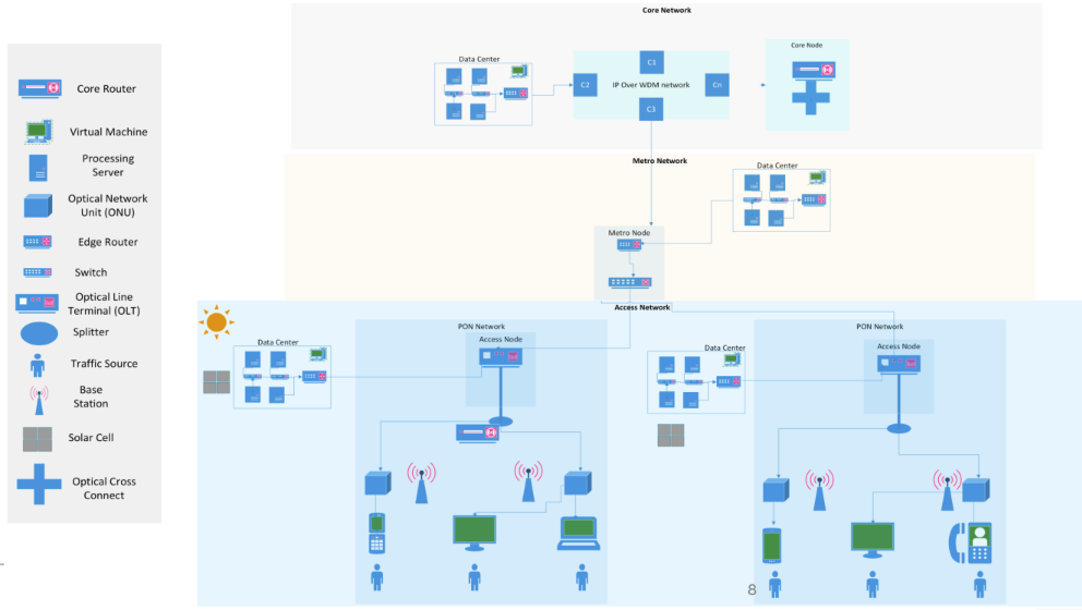
Figure 2: Cloud to fog architecture with solar power consideration.

VMs provide IaaS, PaaS, and SaaS cloud functionalities via VM categories such as Hardware Virtual Machine (HVM), allowing a machine to be virtualized with no operating system, and Container Virtual Machine, allowing multiple secure containers to run different applications on a single kernel, and facilitates user access to containers without interaction with other users. In this paper, Container Virtual Machines will be in consideration as it is the most efficient amongst other virtualization categories [8].

One might wonder, to what extent running a virtual machine on a host machine would affect power consumption compared to running it on native hardware. The difference in power consumption is minuscule and, therefore negligent [9]. This is because many of the virtualized services, such as the operating system and functionality, can be directly processed by the underlying host. Several papers have discussed different approaches to ensure virtualization and allocation are performed to ensure minimal power expenditure in mind. In [10], the authors propose an algorithm, that reduces the number of nodes, based on best-fit, in which VMs with a certain threshold of high traffic are placed on the same host machine to reduce traffic. The algorithm traverses through a list of available VMs, for each VM it searches for available computing nodes that can allocate it, if none is available, then a new computing node is allocated.

An under-utilized server can consume up to 70% of run-time power [11]. In [12], the authors investigate the dynamic reallocation of VMs according to CPU usage. This in turn becomes a bin-packing problem, where VMs are always evaluated on the basis of whether they should be placed in other nodes and their current node needs to be switched off. The power consumption of the processing unit of the underlying server is directly proportional to the workload imposed on the VMs [13], with the CPU component utilizing a greater portion of power compared to the storage and networking functions of the server. Therefore, this paper will consider two work profiles, constant and linear CPU workload profiles.

As data center components, such as routers, switches, and servers, etc. become more prone to failure with increased traffic [14], VM replication schemes have been widely adopted to increase overall redundancy and distribute workload tasks. Related research in this area focus primarily on the server consumption with hosting VMs, however, this work considers the power consumption of additional networking components such as routers and switches. It must be noted that this work only considers the CPU capacity, and not the limitations with the storage capacity of the server.

The consideration of renewable energy in the cloud-to-fog architecture has gained recent attention. In [5], the authors propose a solution, based on the Lyapunov Optimization Technique, that adopts the concept of a request dispatching controller in which all requests are dispatched to. The controller then dispatches requests to nodes that meet the minimum service time and are powered by sufficient green- energy, powered by solar cells. In [15], the authors develop an MILP model, where the effects of wind farms on the locations of clouds and content replication of the clouds are studied. The model identifies the number and locations of clouds given the current number of requests, the transport network power consumption incurred by having user requests processed at the new cloud location, and transmission loss of delivering renewable energy from wind farms. In [16], the authors aim to deliver Video-on-Demand (VoD) traffic by minimizing the energy reliance on non-renewable energy sources and maximizing the usage of solar power available to nodes in the access network. Due to the fluctuating nature of solar power energy, energy storage devices (ESD) were utilized to store surplus energy. For the core network, this paper considers IP over WDM bypass and Mixed Line Rate.

III The Proposed System

This paper presents an extension to [17], where the authors develop an MILP model to place virtualized machine (VM) services in different nodes in the cloud-fog architecture for optimum energy efficiency given several factors. These include: the minimum VM minimum workload requirement to operate, the VM popularity, and data rate incurred from traffic. The authors conducted the study on an AT&T cloud fog architecture with fixed traffic rates. This paper demonstrates the impact of placing renewable energy sources, such as solar power, in the access network on the placement of VMs on cloud to fog nodes. We consider the dynamic VM placement given the daily traffic quantities of the BT 21CN network topology shown in Figure 4. We consider the bypass approach of IP over WDM whereas [18] consider the non- bypass approach. Related research such that of [16], acknowledges that solar power energy is heavily reliant on the current forecast and the time of the day, therefore, surplus energy could be stored in either energy storage devices or on the power grid. This work will not consider ESDs due to limited battery shelf life and the process of making ESDs has environmental implications. Although lithium oxides can be recycled, resource depletion and ecotoxicity arise from materials such as copper, cobalt, and silver [19].

III-A Cloud-to-fog Network Design

The Cloud-to-fog network is composed of multiple layers, as indicated in Figure 2, the top is the core network, traversing down to the metro network, and finally to the access network. The core network is composed of the IP nodes over the WDM network, which facilitates the communication throughout the topology. It has two layers, the IP layer, containing core IP routers that provide maximum bandwidth to optimize routing to destination and group data packets based on common traits obtained from low-end edge routers, and an optical layer. Each core IP router is connected to the optical layer that consists of optical switches, which connects to an optical cross connect, which divides shares the bandwidth into multiple wavelengths of different frequencies, used in Frequency division multiplexing, via an associated transponder, that sends fiber data using a single fiber optic. As the network topology spans over a long distance, Erbium-Doped Fiber Amplifiers (EDFAs) are used as amplifiers, this is illustrated by Figure 3. [20] A transponder’s main job in IP over WDM is to convert the the signal received from an IP router into the desired WDM wavelength, and vice-versa at the demultiplexer end. A core network can be composed of several points of presence.

We design the nodes to contain a limited amount of IP routers at a given node and have a maximum amount of wavelengths to a single optical fiber cord. Power consumption that is utilized from the IP routers, optical switches, optical cross-connects, transponders, and EDFAs are summed as part of the objective function, which aims to minimize the total energy consumption stemming from the components. The model ensures that the flow conservation law is satisfied such that the total outgoing flow of data packets is equal to the total incoming flow if the node, or the point of presence, is an intermediate node. [21] If it is a source node, then the total output flow subtracted by the total input flow must be equal to the traffic demand between the node pair. [21] If it is a destination node then the total incoming flow minus the output flow is equal to the traffic demand between the node pair. This law ensures that data packets can be diverged throughout multiple nodes, in both the virtual and physical topologies. The virtual topology consists of a set of light paths that sits on top of the physical layer, this ensures that if a physical node is malfunctioning, then packets are still able to be routed appropriately. The model ensures that sufficient wavelength capacity is available in both the physical and virtual topologies.

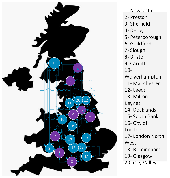
Figure 3: BT 21 CN Network Topology

[22] [23]

A metro network serves as an aggregation layer that connects access network node traffic to the core network. It is consistent of ethernet switches and edge routers. Metro switches are connected to multiple routers to increase redundancy.

The access network connects traffic to backbone network, it is considered the first point of access in which users access via an ONU, where data is forwarded and received by VMs directly. In this work, the GPON, which allows for VoIP, IP, etc. services is the chosen passive-optical network (PON) standard where the optical line terminal (OLT), connected by a single optical fiber, acts as the ISP networking endpoint. This work considers only upstream flow of data, as a downlink traffic is negligent. It is worth noting that other access network technologies such as Asymmetric digital subscriber line (ASDL), which has limited frequency bands, and Fiber to Node (FTTN) [24] [25] which incorporates copper and fiber optic, do exist, however will not be considered as GPON is adopted for the BT 21CN.

It is worth noting that due to the nature of many modern applications, users are not constantly imposing workloads to the network at the access rate stated by the ISP, which means, user time segmented upload workload is received by the network by Time Division Multiplexer. We consider traffic to be imposed only at access rates advertised, and not at variable access rates throughout the day.

III-B Renewable Energy in the Fog Nodes

This work considers solar power as renewable energy as their cell sizes can be configured to be appropriately placed in central offices, located in the PON network (access), near traffic-producing sources. The available solar power is in units of W/m2 and the values presented in Table 2 have been obtained from the SOLPOS calculator based on the BT network node locations.

III-C Datacenter design

Datacenter servers tend to consume up to 70 percent when in an idle state [26]. In order to combat this, VM consolidation is a technique that involves clustering VMs to servers with computing capacity left, however this decreases the performance of the VM. In this work, VM consolidation is not considered, despite its overall power efficiency improvement [27]. In order to maintain QoS, a VM service maintains a base workload load, this occurs from the CPU utilization used to host the OS, in order to provide the IaaS, SaaS, and PaaS services to users that request it. In addition, This workload consists of maintaining the memory footprint and listening to incoming requests from users. In the industry, VM replicas are used to increase service reliability [14] to serve users in nodes, the creation of multiple replicas is due to the fact that the number of users exceeds the maximum capacity a single VM unit can serve. The MILP model would determine the number of replicas needed for a single data center by dividing the total traffic imposed on the VM in the data center and divide it by the maximum number of users and their download rate a single VM can serve. As the number of users increases, the underlying CPU utilization increases in a linear fashion. This is accounted in the MILP model.

Variables

$$W_{jit}^{P}$$ Number of used wavelengths on physical link between nodes at time

Number of fibers on physical link between nodes at time

Wavelengths on the virtual link from nodes at time

Number of wavelength channels between through optical layer physical link at time

Number of wavelengths in the virtual link between the node pair and at time

Packet traffic flow between node pairs through virtual link at time

Number of fibers on virtual link between nodes at time

Number Wavelengths carried by fiber, between nodes at time

Number of router ports in node that aggregate traffic

Number of servers at node

Number of switches in cloud node

Number of router ports in fog data center connected to core node

Number of metro servers at node in the processing server

Number of switches in fog data center connected to core node

Number of metro node routers connected to core node

Number of metro node switches connected to core node

Number of access router ports in fog data center connected to core node

Number of access processing servers at node in data center

Number of access node switches at node in data center

Number of OLTs present in PON network

Number of ONUs connected to an OLT that is present in PON network connected to node

$$RVM_{xist}^{L}$$ Response traffic from the replicated VM unit hosted in the data center in PON (if access node), connected to core node , at time

Binary variable: 1 if a VM replica is hosted in access data center, in PON network , connected to core node at time , else 0

Binary variable in which , if a data center is hosted in network , connected to core node , at PON (if Access Node)

Binary variable in which if a VM replica is hosted in access data center, in PON network , connected to core node at time , else

Total workload by summing all VM replica workloads in node , at PON (if ), at time

Number of servers in data center connected to PON if(), connected to core node

Traffic flow from VM replica , hosted on node to users at time

Number of routers to be installed in data center in layer , connected to node

Number of switches to be installed in data center in layer , connected to node

Number of access router ports in fog data center connected to core node powered by brown sources

Number of access processing servers at node in data center powered by brown power sources

Total number of servers, derived from the number of both brown and green powered

Total number of switches, derived from the number of both brown and green powered

Total number of routers, derived from the number of both brown and green powered

Number of green powered servers at node , at PON

Number of green switches servers at node , at PON

Number of green-powered routers at node , at PON

Total response traffic from all VMs at PON connected at node at time

Parameters

$$C^{PUE}$$ Power Usage Effectiveness of Cloud

Distance between EDFAs (KM)

Physical link distance, between the nodes in N (KM)

Time of day (HR)

Set of IP over WDM nodes

. Number of EDFAs on the physical link between from

EDFA Power Consumption (W)

Power Consumption of a Transponder (W)

Router Port Power Consumption (W)

Number of router ports that aggregate traffic from metro routers at node

Traffic between node pair at time

Wavelength data rate or capacity (Gb/s)

Cloud Fog Router Power Consumption (W)

Cloud Switch Power Consumption (W)

Switch Redundancy cloud and fog

Cloud Data Center Power Usage Effectiveness

Server Power Consumption (W)

Power consumption of core network (W)

Power consumption of cloud servers (W)

Power consumption of cloud routers and switches (W)

$$M^{RP}$$ Metro Router Power Consumption (W)

Metro Switch Power Consumption

Metro Fog Redundancy

Metro Node Router Power Consumption

Metro Node Switch Power Consumption

Metro Node Redundancy

Metro Data Center Power Usage Effectiveness

Access fog router power consumption

Access fog switch power consumption

OLT power Consumption

ONU power consumption

Access Data Center Power Usage Effectiveness

Access Data Center Switch

Traffic flow from VM to users in PON connected to core node , at time

OLT Capacity at PON , connected to node

Broadband rate

Number of users at PON , connected to node accessing VM replica , at time

User download rate

$$Z$$ Very Large Number

Maximum workload of VM

Minimum workload requirement for VM . This equation represents workload per traffic unit

$$USER_{x}^{D}$$ User data rate accessing VM

Maximum number of users VM can support

Minimum workload requirement

IV MILP Model

Objective Function: Minimize

The objective of the MILP model is to minimize the total energy consumption, derived from non-renewable sources (grid), therefore the model will reduce the amount of servers, routers, switches, ONUs, and OLTs used in the network

$$P_{CN}=P_{\text{transponder}}+P_{\text{EDFA}}+P_{\text{routerPort}}$$ (1)

$$P_{transponder}=\Sigma_{j\epsilon N}\Sigma_{i\epsilon N_{m}}W_{jit}T^{p}(t)$$ (2)

$$P_{\text{EDFA}}=\sum_{t\in T}\sum_{j\in N}\sum_{i\in N_{m}}EDFA^{P}\left({\frac{D_{ij}}{S-1}+{2}}F^{P}_{mnt}\right)$$ (3)

$$P_{\text{routerPort}}=\sum_{j\in N}RP^{P}\left(RPs+\sum_{t\in T}\sum_{\begin{subarray}{c}i\in N\\ j\neq i\end{subarray}}W^{V}_{jit}\right)$$ (4)

$$PWR=P_{Metro}+P_{Core}+P_{Access}$$ (5)

$$\begin{split}P_{Core}=&\ P_{CS}\\ &+P_{CSR}\\ &+P_{CN}\end{split}$$ (6)

$$P_{CSR}=\sum_{t\in T}\sum_{z\in N}C^{\text{RP}}C_{z}^{\text{RA}}+(C^{\text{SWP}}C_{z}^{\text{SA}})$$ (7)

$$P_{CS}=C^{\text{PUE}}\sum_{t\in T}\sum_{z\in N}C_{z}^{\text{AS}}S^{P}$$ (8)

$$\text{CoreNetwork}=P_{\text{transponder}}+P_{\text{EDFA}}+P_{\text{routerPort}}$$ (9)

$$\text{MetroP}_{\text{datacenter}}=\text{MetroP}_{\text{server}}+\text{MetroP}_{\text{datacenterRouterSwitches}}$$ (10)

$$\text{MetroP}_{\text{server}}=M^{\text{PUE}}\sum_{z\in N}M_{z}^{\text{AS}}S^{P}$$ (11)

$$\text{MetroP}_{\text{datacenterRouterSwitches}} = \sum_{t\in T}\sum_{z\in N}\left(M^{\text{RP}}M_{z}^{\text{RA}}\right)$$ (12)

$$\quad+M^{\text{SWP}}MF^{\text{R}}M_{z}^{\text{SA}}$$

$$\text{MetroP}_{\text{router}}=\sum_{z\in N}\text{MN}^{\text{RP}}\text{MN}^{R}{\text{MN}}_{z}^{\text{AR}}$$ (13)

$$\text{MetroP}_{\text{switch}}=\sum_{z\in N}\text{MN}^{\text{SWP}}\text{MN}_{z}^{\text{ASW}}$$ (14)

$$\text{AccessP}=\text{AccessP}_{\text{datacenter}}+P^{\text{ONU}}+P^{\text{OLT}}$$ (15)

$$\text{AccessP}_{\text{datacenter}}=\text{AccessP}_{\text{server}}+\text{AccessP}_{\text{datacenterRouterSwitches}}$$ (16)

$$\text{AccessP}_{\text{server}}=A_{\text{PUE}}\sum_{z\in N}A_{z}^{\text{BASS}}P$$ (17)

$$\text{AccessP}_{\text{datacenterRouterSwitches}} = \sum_{t\in T}\sum_{z\in N}\Big{(}A^{\text{RP}}A_{z}^{\text{BRA}}$$ (18)

$$+\>A^{\text{SWP}}AF^{\text{R}}A_{z}^{\text{BSA}}\Big{)}$$

$$P_{OLT}=\sum_{i\in P}\sum_{z\in N}OLT^{P}(OLT_{iz}^{A})$$ (19)

$$P_{ONU}=\sum_{i\in P}\sum_{z\in N}ONU^{P}(ONU_{iz}^{A})$$ (20)

Constraints

$$\sum_{s\in N}\sum_{d\in N}P_{ijt}^{sd}\leq W_{ijt}^{P}F_{ijt}^{P},\quad i\in N,j\in N_{m},t\in T:i\neq j$$ (21)

Constraint (21) Maintains traffic quantity under physical link capacity

$$\sum_{s\in N}\sum_{d\in N}V_{ijt}^{sd}\leq W_{ijt}^{V}WN,\quad i,j\in N,t\in T:s\neq d$$ (22)

Constraint (22) Maintains traffic quantity under virtual link capacity

$$\begin{split}\sum_{\begin{subarray}{c}i\in N\\ i\neq j\end{subarray}}V_{jit}^{sd}-\sum_{\begin{subarray}{c}i\in N\\ i\neq j\end{subarray}}V_{ijt}^{sd}&=\left\{\begin{array}[]{ll}T_{t}^{sd}&\text{if }m=s\\ -T_{t}^{sd}&\text{if }m=d\\ 0&\text{otherwise}\end{array}\right.\\ &\quad\forall s,d,j\in N,\>\forall t\in T,\>s\neq d\end{split}$$ (23)

Constraint (23) maintains the flow conservation law in the core network virtual link. It ensures that packets are directed from the source to the destination. If the router is an intermediate router, then the incoming traffic is equal to the outgoing traffic

$$\begin{split}\sum_{j\in N_{m}}PT_{ijt}^{sd}-\sum_{j\in N_{m}}PT_{jit}^{sd}&=\left\{\begin{array}[]{ll}W_{ijt}^{V}&\text{if }i=s\\ -W_{ijt}^{V}&\text{if }i=d\\ 0&\text{else}\end{array}\right.\\ &\quad\forall t\in T,\;\forall s,d,i\in N,\;i\neq d\end{split}$$ (24)

Constraint (24) Maintains the physical flow conservation law in which incoming multiplexed wavelengths are either absorbed or sent.

$$\sum_{i\in P}\sum_{d\in N}RT_{xidt} = \sum_{s\in N}\sum_{i\in P}RVM_{xist}^{A}+\sum_{s\in N}RVM_{xst}^{M}$$ (25)

$$+\>\sum_{s\in N}\sum_{d\in N}RVM_{xsdt}^{C},$$

$$\quad\forall x\in VM,\>\forall t\in T$$

Constraint (25) ensures that the demand from traffic-producing sources is satisfied with a VM in a data center in a core network and/or a replica VM in a data center in a metro and PON networks

$$\begin{split}RT_{xidt}&=USER_{xidt}\cdot USER_{x}^{D},\\ &\quad\forall x\in VM,\>\forall t\in T,\>\forall d\in N,\>\forall i\in P\end{split}$$ (26)

Constraint (26) calculates the maximum bit rate imposed by the maximum amount of users a single VM replica can handle

$$\begin{split}RVM_{xist}^{A}&\geq A_{ixst}^{VM},\\ &\forall i\in P,\>\forall t\in T,\>\forall s\in N,\>\forall x\in VM\end{split}$$ (27)

$$\begin{split}RVM_{xist}^{A}&\leq A_{ixst}^{VM}Z,\\ &\forall i\in P,\>\forall t\in T,\>\forall s\in N,\>\forall x\in VM\end{split}$$ (28)

$$\begin{split}RVM_{xst}^{M}&\geq M_{xst}^{VM},\\ &\forall t\in T,\>\forall s\in N,\>\forall x\in VM\end{split}$$ (29)

$$\begin{split}RVM_{xst}^{M}&\leq M_{xst}^{VM}Z,\\ &\forall t\in T,\>\forall s\in N,\>\forall x\in VM\end{split}$$ (30)

$$\begin{split}Z\sum_{d\in N}RVM_{xsdt}^{C}&\geq C_{xst}^{VM},\\ &\text{for }\forall x\in VM,\>\forall t\in T,\>\forall s\in N\end{split}$$ (31)

$$\begin{split}\sum_{d\in N}RVM_{xsdt}^{C}&\leq C_{xst}^{VM}Z,\\ &\forall t\in T,\>\forall s\in N,\>\forall x\in VM\end{split}$$ (32)

Constraints (27-32) simulate the placement of a VM in a metro, PON and core networks

$$\sum_{x\in VM}A_{ixs}^{VM}\geq A_{si}^{DC},\quad s\in N,\quad i\in P$$ (33)

$$\sum_{x\in VM}A_{ixs}^{VM}\leq A_{si}^{DC}Z,\quad s\in N,\quad i\in P$$ (34)

$$\sum_{x\in VM}M_{xs}^{VM}\geq M_{s}^{DC},\quad s\in N,\quad i\in P$$ (35)

$$\sum_{x\in VM}M_{xs}^{VM}\leq M_{s}^{DC}Z,\quad s\in N,\quad i\in P$$ (36)

$$\sum_{x\in VM}C_{xs}^{VM}\geq C_{s}^{DC},\quad s\in N,\quad i\in P$$ (37)

$$\sum_{x\in VM}C_{xs}^{VM}\leq C_{s}^{DC}Z,\quad s\in N,\quad i\in P$$ (38)

Constraints (33-38) simulate the placement of a datacenters, that are able to host VM services, in the core, metro, and PON nodes.

$$\text{USER}_{x}^{MD}=\text{USER}_{x}^{D}\text{USER}_{x}^{m},\quad x\in VM$$ (39)

Constraint (39) calculates the maximum bit rate imposed by the maximum amount of users a single VM replica can handle

$$A_{xst}^{TVM} = \frac{VM_{x}^{maxW}-VM_{x}^{minW}}{USER_{x}^{MD}\cdot RVM_{xst}^{A}}+A_{xst}^{VM}$$ (40)

$$\times\left(\frac{RVM_{xsdt}^{A}}{USER_{x}^{MD}}\right),$$

$$\quad\forall t\in T,\>\forall x\in VM,\>\forall s\in N,\>\forall i\in P$$

$$M_{xst}^{TVM} = \frac{(VM_{x}^{maxW}-VM_{x}^{minW})RVM_{xst}^{M}}{USER_{x}^{MD}}$$ (41)

$$+\>M_{xst}^{VM}M\frac{RVM_{xsdt}^{M}}{USER_{x}^{MD}},$$

$$\quad\forall t\in T,\>\forall x\in VM,\>\forall s\in N$$

$$C_{xst}^{TVM} = \frac{(VM_{x}^{maxW}-VM_{x}^{minW})}{USER_{x}^{MD}}\sum_{d\in N}{RVM_{xsdt}^{C}}$$ (42)

$$+C_{xst}^{VM}M\sum_{d\in N}\frac{RVM_{xsdt}^{C}}{USER_{x}^{MD}},$$

$$\quad\forall t\in T,\>\forall x\in VM,\>\forall s\in N,\>\forall i\in P$$

$$A_{xst}^{TVM} = VM_{x}^{maxW}A_{xst}^{VM},$$ (43)

$$\quad\forall t\in T,\>\forall x\in VM,\>\forall s\in N$$

$$M_{xst}^{TVM} = VM_{x}^{maxW}M_{xst}^{VM},$$ (44)

$$\quad\forall t\in T,\>\forall x\in VM,\>\forall s\in N$$

$$C_{xst}^{TVM} = VM_{x}^{maxW}C_{xst}^{VM},$$ (45)

$$\quad\forall t\in T,\>\forall x\in VM,\>\forall s\in N$$

Constraints (40-42) calculate the total workload of a single VM placed in a data center that is hosted in a metro network node, a PON network node, or a core node. These constraints consist of two parts. The first part calculates the linear correlation of CPU utilization based on the number of users based on workload per traffic unit. The second part calculates the number of replicas needed in the data center based on the total workflow imposed on the data center and constraint (40). Constraints (43-45), calculate the workload of a VM under a constant CPU profile

$$VM_{ist}^{TWA} = \sum_{x\in VM}A_{xst}^{TVM},$$ (46)

$$\quad\forall t\in T,\>\forall x\in VM,\>\forall s\in N,\>\forall i\in P$$

$$VM_{st}^{TWM}=\sum_{x\in VM}M_{xst}^{TVM},\quad t\in T,\quad x\in VM,\quad s\in N$$ (47)

$$VM_{st}^{TWC} = \sum_{x\in VM}C_{xst}^{TVM},$$ (48)

$$\quad\forall t\in T,\>\forall x\in VM,\>\forall s\in N,\>\forall i\in P$$

Constraints (46-48), calculates the total workloads from the traffic by summing all the workloads of the VM replicas hosted in the datacenters located in the access, metro and core networks

$$\frac{VM_{xizt}^{TWA}}{S^{\text{max}}}\leq A_{is}^{AS},\quad i\in P,\quad s\in N$$ (49)

$$\frac{VM_{xst}^{TWM}}{S^{max}}\leq M_{s}^{AS},\quad s\in N$$ (50)

$$\frac{VM_{xst}^{TWC}}{S^{max}}\leq C_{s}^{AS},\quad s\in N$$ (51)

Constraints (49-51) calculate the number of servers needed each data center of the cloud fog network. The calculations are derived from the total workload imposed on the nodes divided by the maximum workload capacity a server can handle. A VM service utilizes the underlying server’s CPU

$$\begin{split}\frac{\sum_{x\in VM}RVM_{xst}^{A}}{A^{RBR}}&\leq A_{is}^{AR},\\ &\forall s\in N,\>\forall i\in P,\>\forall t\in T\end{split}$$ (52)

$$\frac{\sum_{s\in N}\sum_{v\in VM}RVM_{xst}^{C}}{C^{RBR}}\leq C_{s}^{AR},\quad s\in N$$ (53)

$$\frac{\sum_{x\in VM}RVM_{xst}^{M}}{M^{RBR}}\leq M_{s}^{AR},\quad s\in N$$ (54)

Constraints (52-54) calculate the number of routers needed each data center of the cloud fog network. The calculations are derived from the total traffic imposed on the nodes divided by the bit rate of the respective routers

$$\frac{\sum_{v\in VM}RVM_{xst}^{A}}{ASWB}\leq A_{is}^{ASW},\quad s\in N,\quad i\in P,\quad t\in T$$ (55)

$$\frac{\sum_{d\in N}\sum_{v\in VM}RVM_{xst}^{C}}{CSWB}\leq C_{s}^{ASW},\quad s\in N$$ (56)

$$\sum_{v\in VM}\frac{RVM_{xst}^{M}}{MSWB}\leq M_{s}^{ASW},\quad s\in N$$ (57)

Constraints (55-57) calculate the number of switches needed each data center of the cloud fog network. The calculations are derived from the total traffic imposed on the nodes divided by the bit rate of the respective routers

We now introduce novel constraints to the model to ensure green power is dedicated to routers, switches, and serves in the access fog data center:

$$A_{is}^{AS}=A_{is}^{AGS}+A_{is}^{BAS},\quad i\in P,s\in N$$ (58)

Constraint (58) Indicates the total number of servers in an access fog, in PON network i, connected to node z, is consistent with servers powered by both green and non-renewable energy

$$A_{\text{is}}^{\text{ASW}}=A_{\text{is}}^{\text{AGSW}}+A_{\text{is}}^{\text{BASW}},\quad i\in P,s\in N$$ (59)

Constraint (60) Indicates the total number of routers in an access fog, in the PON network i, connected to node z is consistent of servers powered by both green and non-renewable energy

$$A_{\text{is}}^{\text{AR}}=A_{\text{is}}^{\text{AGR}}+A_{\text{is}}^{\text{BAR}},\quad i\in P,s\in N$$ (60)

Constraint (59) Indicates the total number of switches in an access fog, in PON network i, connected to node n is consistent of servers powered by both green and non-renewable energy

$$A_{is}^{AGS} = \frac{{SP_{ist}^{m}SP-\left(A_{is}^{AGSW}A^{SWP}+A_{is}^{AGR}A^{RP}\right)}}{S^{P}},$$ (61)

$$\quad\forall t\in T,i\in P,s\in N$$

Constraint (61) Indicates the number of servers at PON p, connected to node z, powered by the available green energy at time t

$$A_{is}^{AGS}\leq\frac{VM_{ist}^{TWA}}{S^{\text{max}}}\quad\forall t\in T,i\in P,s\in N$$ (62)

Constraint (62) Indicates the number of routers at PON p, connected to node z, powered by the available green energy at time t

$$A^{GR} = \frac{{S^{P}_{ist}m^{SP}-\left(A_{is}^{AGS}S^{P}+A^{SWP}A_{is}^{AGSW}\right)}}{{A^{RP}}}$$ (63)

$$,\>\forall t\in T,i\in P,s\in N$$

Constraint (63) Indicates the number of switches at PON p, connected to node z, powered by the available green energy at time t

$$A_{is}^{GR}\leq\frac{{\sum_{x\in VM}RVM_{xist}^{A}}}{{A^{RBR}}}\,\\ ,\forall t\in T,i\in P,s\in N$$ (64)

Constraint (64) Indicates the number of servers at PON p, connected to node z, powered by the available green energy at time t, needs to be less than the total number of servers

$$A_{is}^{AGSW} = \frac{{SP_{ist}^{m}SP-\left(A_{is}^{AGS}S^{P}+A^{RP}A_{is}^{AGR}\right)}}{{A^{SWP}}}$$ (65)

$$,\>\forall t\in T,i\in P,s\in N$$

Constraint (66) Indicates the number of routers at PON p, connected to node z, powered by the available green energy at time t, needs to be less than the total number of routers

$${A_{iz}}$$

$$A_{is}^{AGSW}\leq\sum_{x\in VM}\frac{R^{VMA}_{xist}}{A^{SWB}}\,,\forall t\in T,i\in P,s\in N$$ (66)

Constraint (67) Indicates the number of switches at PON p, connected to node z, powered by the available green energy at time t, needs to be less than the total number of switches In which the number of brown-powered servers, switches, and routers placed in the data centers is minimized by the model.

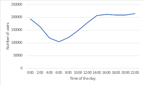
Figure 4: BT 21 CN Average Traffic

V Results

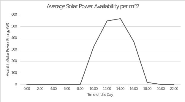
Figure 5: Average Solar Power Availability

Figure 6: Solar Power Availability at Different Nodes (W)

TABLE I: Access Fog Nodes and Access Network Parameters

Parameter	Input Value
PUE of an Access Node	1.5
Access Fog Switch Bit Rate	160 Gbps
Access Fog Switch Power Consumption	102W
Access Router Port Bit Rate	40 Gbps
Access Router Power Consumption	13 W

TABLE II: Metro Fog Nodes and Metro Network Parameters

Parameter	Input Value
PUE of a Metro Node	1.4
Metro Fog Switch Bit Rate	600 Gbps
Metro Fog Switch Power Consumption	470 W
Metro Fog Router Bit Rate	600 Gbps
Metro Fog Router Power Consumption	13W
Metro Network Node Router Bit Rate	40 GBps
Metro Network Node Power Consumption	30W
Metro Network Switch Bit Rate	384 Gbps
Metro Network Switch Power Consumption	55 W
Metro Fog Router Port Bit rate	40 Gbps

TABLE III: Core Network Inputs

Parameter	Input Value
Number of Wavelengths per fiber between (m, n)	32
Wavelength data rate	40 GBps
Maximum Distance between two EDFAs in km	80 km
Power consumption of an EDFA	55 W
Power consumption of a Transponder	167 W
Power Consumption of an IP router in the core network	638 W
PUE of a Cloud Node	1.3
Cloud Fog Switch Bit Rate	600 Gbps
Cloud Fog Switch Power Consumption	470 W
Cloud Fog Router Bit Rate	40 GBps
Cloud Fog Router Power Consumption	30W
Cloud router Port Bit Rate	40Gbps

TABLE IV: General Parameters

Parameter	Input Value
Server Power Consumption	450 W
Maximum Server Workload	100%
Metro Network Node Router Redundancy	2

TABLE V: VM Input

Parameter	Input Value
Number of Virtual Machines	1
User download rate from accessing VM x	{2 MBps}
Maximum number of users VM x can serve	640
Percentage of underlying CPU that VM x utilizes for its maximum workload capacity	{2%, 50%}
Minimum workload of VM x when no traffic is imposed	30%

TABLE VI: PON Network Input

Parameter	Input Value
Power Consumption of an OLT	1842 W
OLT Capacity located in PON i linked to node z	1280 Gbps
Number of OLTs present in PON network p	1
Power consumption of an ONU	5 W

In the cloud-to-fog, the power consumption of networking components varies, where components such as switches in the cloud and core networks consume greater power, and switches in the access networks tend to consume less power. The BT 21 CN network topology consists of 20 nodes and 68 bidirectional links as demonstrated in Figure 3. A node is an IP core router that supports multiple routing protocols and is connected via an optical switch to other nodes in the backbone. A node connects to the metro network via edge routers connected to the broadband network gateway. The access network is accessed via an ethernet switch connected to an OLT, which supports ONUs that allow users to access the network. Figure 4 indicates the varying traffic quantity over a day period obtained in 2016 [28]. According to [29], a list of networking vendors provide networking equipment for the BT 21 CN. This includes Cisco and Lucent for the backbone core nodes. Alcatel, Siemens, and Alcatel for the metro switches and edge routers. Ciena for the optical fibers that allow for the IP over WDM. Fujitsu for access network supplier. As the BT 21 CN topology utilizes the Dense-Wavelength Division Multiplexing (DWDM) the backbone, the Cisco CRS-1 Carrier Routing System is the adopted core IP router that provides for 40 Gbps throughput at 638 W of power, that provides routing of voice, data, and video induced to VMs.The Cisco IOS CR7 [30] is the adopted network operating system, therefore, the edge router located in the metro network is routed via the Cisco NCS-5502-SE Chassis with 30 W power consumption per 40 Gbps router port and is connected to the CRS-1 via a packet over SONET 10 Gbps link. The Cisco NCS-5502 is the router adopted in the data centers located in the metro and access networks, where 30 W of power is consumed per 40 Gbps. The Alcatel-Lucent OmniSwitch 6450 is the adopted switch for the data centers which consume 102 W of power and has a bit rate of 162 Gbps. This work considers tree-and-branch PON topology to connect users to the network. An optical fiber, provided by Ciena, connects to a splitter that splits the fiber link to time-shared user ONUs. The Wave7 ONT-G1000i is the adopted ONU, which consumes 5W of power, and communicates with the Hitachi 1220 OLT device, which consumes 1842 W of power. The MILP models in this paper have been solved on an AMD Ryzen 7 4800H with 8 Core CPUs.

Figure 8 illustrates the number of wavelengths needed in the physical and virtual links in order to fulfill traffic. Figure 7 indicates a linear increase in power consumption with increased traffic demand. The results show that IP routers consume almost 90 percent of the total power consumption, whilst EDFAs, Optical Cross Connects, etc. consume a smaller portion in the core node. This is due to the fact that IP routers are directly managing user traffic with multiple routing algorithms [31].

We investigate the optimal VM placement, given different workloads and VM workload profiles throughout the day at time t, with renewable energy placed in the access data centers. We do not consider VM replication as the primary reason for increasing redundancy and acknowledge that replicas throughout the network may not be consistent. The results indicate that the VM placement varies due to the amount of traffic.

Three workload profiles: 25 percent, 50 percent, and 100 percent of the underlying CPU capacity of the host server, workload profile (constant or linear), and user data rates of 2 Mbps, which for the most part satisfies basic user tasks such as social media, text messaging, etc. Ideal PUE values of 1.5, 1.4, and 1.3 for the core, metro, and access networks where utilized [32].

Figures 12,13 show Under the constant workload, it was indicated that as the workload of VMs decreases, from decreased traffic demand, more VM replication occurs in the metro and access fogs. This is due to the fact that computing resources in the fog layers are limited, which is sufficient for VMs with small workloads. This is the opposite case for periods of increased traffic where VMs are placed in the clouds, whereas the VMs are allowed more computational resources.

Under the linear workload, it has also been shown that workload is proportional to traffic, Figures 9, 10, and 11 demonstrate the VM placement in which the user data is 2 Mbps, and indicate the same behavior, however, lesser offloading to access and metro layers. The total power consumption, under a linear workload, with a minimum of 2 percent CPU utilization profile (to maintain QoS, and OS, etc.). The figure indicates that user traffic is proportional to power overall consumption.

It is clear that whenever solar power was high, between 12:00 – 16:00, VM replicas tended to be placed on the access nodes. This is due to the reason that the overall PUE of the access data center improved. In addition, transport cost is saved with the addition of solar power. Under constant workload, VMs were placed primarily in clouds whenever solar power was not available and were placed in access data centers whenever solar power was available. VM replicas are placed towards the access fog data centers whenever traffic and user data rate is increased. This means that the MILP accounted for the fact that an increased number of users requesting core data centers is less efficient. Under the linear workload, VM replicas tended to be placed in the access nodes as VM workload decreased. Whenever traffic was high, VMs were placed in the cloud and metro nodes. Overall power consumption was reduced by 16 percent as indicated in Figure 15 compared to Figure 14, where no solar power was noticed, this is noticeable in times 10:00 – 14:00, where solar power was high, and user the data rate was relatively low.

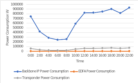
Figure 7: Power consumption of various core node components due to varying daily traffic

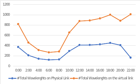
Figure 8: Number of wavelengths a physical and virtual link utilized due to varying daily traffic

Figure 9: VM Placement in Cloud Fog under linear workload, 25 percent VM workload, and user download rate of 2 Mbps

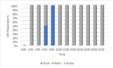
Figure 10: VM Placement in Cloud Fog under linear workload, 50 percent VM workload, and user download rate of 2 Mbps

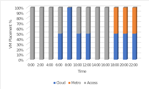
Figure 11: VM Placement in Cloud Fog under linear workload, 100 percent VM workload, and user download rate of 2 Mbps

Figure 12: VM Placement in Cloud Green Fog under constant workload, 50 percent VM workload, and user download rate of 2 Mbps

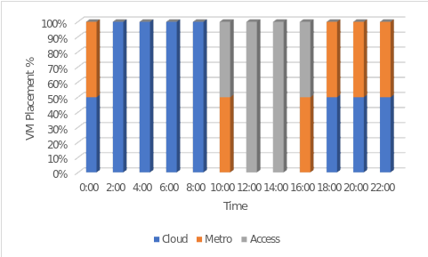
Figure 13: VM Placement in Cloud Green Fog under constant workload, 25 percent VM workload, and user download rate of 2 Mbps

Figure 14: Overall Power consumption with only brown energy consideration

Figure 15: Overall Power consumption with solar energy consideration

VI Conclusion

There are clear advantages to the use of solar power in the fog layer, especially when considering virtual machine (VM) placement in a topology such as BT’s 21st Century Network (21 CN). We have demonstrated that nodes powered by solar energy have been found to have more VM placement, therefore, providing lower latency rates to nearby users. This paper demonstrates one aspect of renewable energy solutions in network infrastructures by this notable improvement compared to other models in the field that solely depend on conventional ’brown’ power sources.

References

- [1] I. Odun-Ayo, O. Ajayi, and C. Okereke, “Virtualization in cloud computing: Developments and trends,” in 2017 International Conference on Next Generation Computing and Information Systems (ICNGCIS), Jammu, India, 2017, pp. 24–28.
- [2] International Energy Agency (IEA), “Global energy review: Co2 emissions in 2021 – analysis,” [Online]. Available: https://www.iea.org/reports/global-energy-review-co2-emissions-in-2021, 2022.
- [3] Z. Qu, Y. Wang, L. Sun, D. Peng, and Z. Li, “Study qos optimization and energy saving techniques in cloud, fog, edge, and iot,” Complexity, vol. 2020, 2020. [Online]. Available: https://doi.org/10.1155/2020/8964165
- [4] D. Ali Kumar, S. Newaz, F. Rahman, G. Lee, G. Karmakar, and T.-W. Au, “Green demand aware fog computing: A prediction-based dynamic resource provisioning approach,” Electronics, vol. 11, p. 608, 2022. [Online]. Available: https://www.mdpi.com/2079-9292/11/4/608
- [5] T. Cui, Y. Hu, B. Shen, and Q. Chen, “Task offloading based on lyapunov optimization for mec-assisted vehicular platooning networks,” Sensors, vol. 19, no. 22, p. 4974, Nov 2019.
- [6] A. Musaddiq, Y. Zikria, and e. a. Zulqarnain, “Routing protocol for low-power and lossy networks for heterogeneous traffic network,” Journal of Wireless Communications and Network, vol. 2020, no. 21, 2020. [Online]. Available: https://doi.org/10.1186/s13638-020-1645-4
- [7] R. Hat, “Iaas vs. paas vs. saas,” https://www.redhat.com/en/topics/cloud-computing/iaas-vs-paas-vs-saas, Aug 2022.
- [8] Q. Zhang, L. Liu, C. Pu, Q. Dou, L. Wu, and W. Zhou, “A comparative study of containers and virtual machines in big data environment,” arXiv, 2018. [Online]. Available: https://ar5iv.org/abs/1807.01842
- [9] J. Stoess, C. Lang, and F. Bellosa, “Energy management for hypervisor-based virtual machines,” in 2007 USENIX Annual Technical Conference, 2007. [Online]. Available: https://www.usenix.org/legacy/event/usenix07/tech/full_papers/stoess/stoess_html/index_old.html
- [10] P. Khani, B. Tang, J. Han, and M. Beheshti, “Power-efficient virtual machine replication in data centers,” 2022, accessed: March 06, 2022. [Online]. Available: https://csc.csudh.edu/btang/papers/vmr.pdf.
- [11] D. Meisner, B. Gold, and T. Wenisch, “Powernap: Eliminating server idle power,” Accessed: May 06, 2022. [Online]. Available: https://web.eecs.umich.edu/~twenisch/papers/asplos09.pdf, 2009.
- [12] N. G. et al., “Enhanced virtualization-based dynamic bin-packing optimized energy management solution for heterogeneous clouds,” Mathematical Problems in Engineering, vol. 2022, p. e8734198, Jan 2022.
- [13] L. Ismail and H. Materwala, “Eatsvm: Energy-aware task scheduling on cloud virtual machines,” in Procedia Computer Science, vol. 135, 2018, pp. 248–258.
- [14] F. Machida, M. Kawato, and Y. Maeno, “Redundant virtual machine placement for fault-tolerant consolidated server clusters,” in Proceedings of the 12th IEEE/IFIP Network Operations and Management Symposium (NOMS), mini conference, 2010.
- [15] A. Q. Lawey, T. E. H. El-Gorashi, and J. M. H. Elmirghani, “Renewable energy in distributed energy efficient content delivery clouds,” in 2015 IEEE International Conference on Communications (ICC), Jun. 2015.
- [16] M. B. A. Halim, S. H. Mohamed, T. E. H. El-Gorashi, and J. M. H. Elmirghani, “Fog-assisted caching employing solar renewable energy for delivering video on demand service,” in 2019 21st International Conference on Transparent Optical Networks (ICTON), Jul. 2019.
- [17] H. Alharbi, T. El-Gorashi, and J. Elmirghani, “Energy efficient virtual machine services placement in cloud-fog architecture,” in 2019 21st International Conference on Transparent Optical Networks (ICTON), 2019.
- [18] G. Shen and R. Tucker, “Energy-minimized design for ip over wdm networks,” Journal of Optical Communications and Networking, vol. 1, no. 1, p. 176, 2009.
- [19] S. Kim, V. I. Hegde, Z. Yao, Z. Lu, M. Amsler, J. He, S. Hao, J. R. Croy, E. Lee, M. M. Thackeray, and C. Wolverton, “Title of the article,” ACS Applied Materials & Interfaces, vol. 10, no. 16, pp. 13 479–13 490, 2018.
- [20] M. Osman and I. Musa, “Energy efficient ip over wdm networks using network coding,” 2016, accessed: May 06, 2022. [Online]. Available: https://etheses.whiterose.ac.uk/16644/1/ThesisFinalAllCorrections.pdf.
- [21] A. Bressan and K. T. Nguyen, “Conservation law models for traffic flow on a network of roads,” Networks and Heterogeneous Media, vol. 10, no. 2, pp. 255–293, Apr. 2015.
- [22] H. Alharbi, M. Musa, T. El-Gorashi, and J. Elmirghani, “Real-time emissions of telecom core networks,” in 2018 20th International Conference on Transparent Optical Networks (ICTON), 2018.
- [23] Kitz, “21cn - the next generation network,” https://kitz.co.uk/adsl/21cn_network.html, 2023.
- [24] L. Cobo, S. Chamberland, and A. Ntareme, “Low cost fiber-to-the-node access network design,” in 2012 15th International Telecommunications Network Strategy and Planning Symposium (NETWORKS), Oct. 2012.
- [25] R. Baliga, R. Ayre, K. Hinton, W. Sorin, and R. Tucker, “Energy consumption in optical ip networks,” Journal of Lightwave Technology, vol. 27, no. 13, pp. 2391–2403, 2009, accessed: May 4, 2022.
- [26] L. A. Barroso and U. Hölzle, “The case for energy-proportional computing,” IEEE Computer, 2007.
- [27] R. Kumar, S. K. Khatri, and M. J. Diván, “Power usage efficiency (pue) optimization with counterpointing machine learning techniques for data center temperatures,” International Journal of Mathematical, Engineering and Management Sciences, vol. 6, no. 6, pp. 1594–1611, Dec. 2021.
- [28] H. A. Alharbi, M. Musa, T. E. H. El-Gorashi, and J. M. H. Elmirghani, “Real-time emissions of telecom core networks,” in 2018 20th International Conference on Transparent Optical Networks (ICTON), Jul. 2018.
- [29] N. World, “Bt names vendors for 21st century network,” https://www.networkworld.com/article/2320210/bt-names-vendors-for-21st-century-network.html, accessed: [Insert Access Date Here].
- [30] “Cisco network convergence system 5500 series: Fixed chassis data sheet,” https://www.cisco.com/c/en/us/products/collateral/routers/network-convergence-system-5500-series/datasheet-c78-737935.html, accessed: May 06, 2022.
- [31] W. Van Heddeghem et al., “Evaluation of power rating of core network equipment in practical deployments,” in 2012 IEEE Online Conference on Green Communications (GreenCom), 2012, accessed: February 6, 2022.
- [32] R. Zoie, R. D. Mihaela, and S. Alexandru, “An analysis of the power usage effectiveness metric in data centers,” in 2017 5th International Symposium on Electrical and Electronics Engineering (ISEEE), 2017.