Central limit theorems for Fréchet means
on stratified spaces

Abstract.

Fréchet means of samples from a probability measure $\mu$ on any smoothly stratified metric space $\mathcal{M}$ with curvature bounded above are shown to satisfy a central limit theorem (CLT). The methods and results proceed by introducing and proving analytic properties of the escape vector of any finitely supported measure $\delta$ in $\mathcal{M}$, which records infinitesimal variation of the Fréchet mean ${\bar{\mu}}$ of $\mu$ in response to perturbation of $\mu$ by adding the mass $t\delta$ for $t\to 0$. The CLT limiting distribution $\mathcal{N}$ on the tangent cone $T_{\bar{\mu}}\mathcal{M}$ at the Fréchet mean ${\bar{\mu}}$ is characterized in four ways. The first uses tangential collapse $\mathcal{L}$ to compare $T_{\bar{\mu}}\mathcal{M}$ with a linear space and then applies a distortion map to the usual linear CLT to transfer back to $T_{\bar{\mu}}\mathcal{M}$. Distortion is defined by applying escape after taking preimages under $\mathcal{L}$. The second characterization constructs singular analogues of Gaussian measures on smoothly stratified spaces and expresses $\mathcal{N}$ as the escape vector of any such Gaussian mass. The third characterization expresses $\mathcal{N}$ as the directional derivative, in the space of measures on $\mathcal{M}$, of the barycenter map at $\mu$ in the (random) direction given by any Gaussian mass. The final characterization expresses $\mathcal{N}$ as the directional derivative, in the space $\mathcal{C}$ of continuous real-valued functions on $T_{\bar{\mu}}\mathcal{M}$, of a minimizer map, with the derivative taken at the Fréchet function $F\in\mathcal{C}$ along the (random) direction given by the negative of the Gaussian tangent field induced by $\mu$. Precise mild hypotheses on the measure $\mu$ guarantee these CLTs, whose convergence is proved via the second characterization of $\mathcal{N}$ by formulating a duality between Gaussian masses and Gaussian tangent fields.

Introduction

Overview

The central limit theorem (CLT) in $\mathbb{R}^{d}$ records how the averages of size $n$ samples are asymptotically distributed as $n$ grows and the differences between the population and empirical averages are rescaled by a factor of $\sqrt{n}$. In nonlinear intrinsic geometric settings, averages are replaced by Fréchet means, which are expected square-distance minimizers [Fré48]. Laws of large numbers for Fréchet means have been known for nearly half a century in great generality for samples from separable metric spaces [Zie77]. However, geometric CLTs have been much less forthcoming, with the first results in smooth settings arriving in the early 2000s [BP03, BP05]. The few CLTs available in singular (that is, non-smooth) contexts occur on spaces built from flat pieces glued together in combinatorial ways [HHL⁺13, BLO13, HMMN15, BLO18, BL18]. Of these, only [BL18], whose CLT occurs on nonnegatively curved spaces glued from right-angled orthants, treats phenomena at singularities in codimension more than $2$.

General stratified sample spaces are considered explicitly in prior research; see [EH19, Section 2.1] and [HMPS20] for apt, comprehensive reviews of the history and literature, including (in the former case) a summary of hypotheses that various known CLTs assume. However, non-smooth variation of Fréchet means and more general descriptors have until now been skirted, as pointed out in [EH19, Remark 2.8(ii)], by either assuming or proving that the relevant descriptor lies in a smooth space—or at least in a smooth part of the space of descriptors. The goal here is to face the singularities head on, treating truly singular variation of empirical Fréchet means in a general geometric context. Even deciphering the form taken by a CLT in the singular setting is a major theoretical stride.

Smooth CLTs proceed by approximating a manifold with its tangent space at the Fréchet mean. The known singular CLTs reduce to linear cases by gluing flat pieces. What should a CLT look like on general non-smooth spaces, where tangent spaces are not linear and no combinatorial gluing or flat pieces are available? Our main results answer this question by

• highlighting appropriate classes of singular spaces and measures on them;

• identifying the “Gaussian” random variables to which suitably rescaled empirical barycenters converge;

• understanding convergence to these distributions; and

• encapsulating how geometry of the space is reflected in the limiting distribution

to formulate and prove the first general CLT for Fréchet means in singular spaces. This paper is the final in a series whose prior three installments develop relevant convex geometry in tangent cones of spaces with curvature bounded above [MMT23a], introduce suitable singular spaces and show how to collapse them onto smooth spaces [MMT23b], and prove preliminary central limiting convergence along tangent rays at singular Fréchet means in these spaces [MMT23c].

Motivations

Our initial impetus to consider CLTs in singular spaces comes from statistics, where increasingly complex (“big”) data are sampled from increasingly complex spaces of data objects; see [HE20, MD21], for example. The spaces parametrize data objects such as phylogenetic and more general trees [BHV01, Hol03, FL⁺13, LSTY17, LGNH21], shapes [Le01, KBCL99], positive semi-definite matrices [GJS17, BP23], or arbitrary mixtures of linear subspaces or more general smooth spaces. Applications arise in disciplines ranging from computer vision [HTDL13] to medical image analysis [PSF20, PSD00], for instance. Despite the wealth of examples, sophisticated statistical techniques based on geometry currently lack mathematical foundations for probability and analysis in singular settings. A non-smooth CLT serves as a crucial first step. Quantitative bounds can then lead, for example, to confidence regions (generalizing [Wil19] for treespace) or singularity hypothesis testing by detecting whether asymptotics in a given dataset behave in smooth or singular ways. In addition, the inverse Hessian (see Section 1.5) is potentially key to generalizing the Cramér–Rao bound on variance in parametric statistics involving families of distributions indexed by manifolds to much more general settings, perhaps including essentially nonparametric settings in which distributions can be selected from more or less arbitrary spaces of measures. This approach could have impact throughout theoretical and applied statistics, including applications to topological data analysis via the space of persistence diagrams [MMH11].

The statistical perspective leads naturally to fundamental probabilistic problems, such as characterizing Gaussian objects in singular settings: do they have alternative interpretations in terms of infinite divisibility, heat dissipation, or random walks on singular spaces [BK01, Bou05, NW14, Nye20]? Again, the spaces in all of these studies of Brownian motion are glued in combinatorial ways from flat pieces, so general foundations are called for to enable unfettered investigations into geometric probability of singularities. Preliminary discussions indicate that singular Gaussians via tangential collapse are pivotal for proving that relevant processes are martingales [AM23].

On the metric geometry side, local features induce curvature that deforms the asymptotics of large samples. In the smooth CLT [BP05], curvature enters as a correction upon passing from a Riemannian manifold to its tangent space at the Fréchet mean, where the asymptotics naturally occur. Turning this observation on its head, understanding asymptotics of large samples furnishes insight into local curvature invariants. The metric geometry of shadows [MMT23a], tangential collapse [MMT23b], and distortion (Section 6.3), for instance, generalize the concept of angle deficit to singularities of stratified $\operatorname{CAT}(\kappa)$ spaces which, when integrated, could yield global topological information. Similarly, any advance on Brownian motion in singular spaces could have topological consequences, in analogy to the smooth setting, where Brownian motion leads to a proof of the Atiyah–Singer index theorem [Hsu88]. Hence another key motivation for this paper is to initiate a program to probe the geometry of singularities via asymptotics of sampling.

This program in singularity theory is especially tantalizing when the singularties are algebraic, as resolution of singularities [Hir64] permits comparison of smooth and singular settings. It suggests a functorial central limit theory that pulls back or pushes forward local sheaf-theoretic information around Fréchet means under dominant algebraic maps to correct for distortion, just as inverse Hessians on Riemannian manifolds (or the distortion map in our singular setting here) corrects the passage from a space to its tangent space. The first step would be to show that CLTs via desingularization agree with CLTs calculated directly on singular spaces, via the methods here, when the spaces satisfy the relevant smoothly stratified hypotheses. Desingularization then extends the theory to all varieties. Such a theory stands in analogy with how multiplier ideals encode their analytic incarnations in terms of locally summable holomorphic germs [Nad90] algebraically as sections of $\mathbb{Q}$-divisors [Dem12, Remark 5.9]. Thinking further along algebraic lines, when samples are taken from a moduli space, so sample points represent algebraic varieties or schemes, a CLT would summarize variation of average behavior in families.

Methods

The leaps required to formulate and derive the singular CLT involve multiple changes in perspective which, taken together, constitute a powerful toolkit for analyzing random variables valued in singular spaces. These include especially

1. comparison of the tangent cone at the population mean with the tangent cones infinitesimally near the population mean [MMT23b] and application of the resulting tangential collapse to push the CLT from a singular to a linear setting;

2. direct geometric construction of the inverse Hessian of the Fréchet function (the distortion map), given that the Hessian itself becomes singular in this setting;

3. interpretation of the CLT as convergence of random tangent fields to a Gaussian random field ray by ray at the Fréchet mean [MMT23c] followed by its transformation, through a variational problem, to full spatial variation about the mean;

4. characterization of the limiting distribution of a measure $\mu$ as the distribution of means after perturbing $\mu$ by adding a singular-Gaussian random measure.

To orient the reader, it may help to discuss these developments in more detail.

To begin, even the transition from sample space to tangent object at the population mean requires novel input in the singular context, namely the introduction [MMT23b] of a new class of singular spaces suitable for central limit theorems. These metric spaces are optimally general: they

• have curvature bounded above in the usual Alexandrov sense [BBI01];

• are stratified in the usual topological sense [GM88]; and

• admit logarithm and exponential maps that are locally inverses of each other, to enable transfer from the original space to the tangent cone.

See Section 2.1–2.2 for a summary of the salient points.

Broadly speaking, the driving theoretical advance here reduces variation of Fréchet means ${\bar{\mu}}_{n}$ of samples $\mu_{n}$ from a population measure $\mu$ to variation of the Fréchet mean ${\bar{\mu}}$ of $\mu$ itself upon perturbing $\mu$ by adding an infinitesimal finitely supported mass $t\delta$ with $t\to 0$. Behavior of the resulting escape vector (§1.4) as a function of $\delta$ is what distinguishes the singular setting from the smooth setting (where escape can be phrased in terms of influence functions; see Remark 6.28). Indeed, in linear settings, adding a point mass $\delta$ to $\mu$ simply causes the mean ${\bar{\mu}}$ to move along a vector pointing toward the support of $\delta$. In smooth settings, local perturbation of $\mu$ in the tangent space behaves similarly, but transferring that motion back from the tangent space to the sample space incurs a distortion quantified by the inverse Hessian of the Fréchet function to capture the average spread rate of geodesics through ${\bar{\mu}}$. In the singular setting of smoothly stratified spaces, the geometry is set up so that local perturbation of $\mu$ in the tangent cone makes sense. But the Hessian is singular: geodesics can branch at ${\bar{\mu}}$. The distortion inherent in transfer from the tangent cone to the sample space therefore requires direct construction of the inverse Hessian (§1.5) rather than proceeding by way of the Hessian itself.

The geometry of distortion on smoothly stratified metric spaces is distinctly singular in nature. As might be expected from branching geodesics, it collapses sectors containing sizable open sets; this is the geometry of shadows [MMT23a] and tangential collapse [MMT23b], which in turn form foundations for the construction of Gaussian objects in singular contexts (§1.6). These Gaussian masses are measures on the tangent cone defined essentially as sections (also known in probabilistic language as selections) of linear Gaussian random variables under tangential collapse.

But, crucially, the limiting distribution in a singular CLT is not Gaussian: rather, it is a type of convex projection of a Gaussian. In the smooth setting, since the tangent space at the Fréchet mean is already linear, distortion is a linear map. The lesson from the singular setting is to interpret that linear map as escape. Thus the limiting distribution of $\mu$ is the escape vector of the Gaussian mass $\Gamma_{\mu}$ constructed from $\mu$ via tangential collapse (Theorem 1 in §1.6).

Beyond producing limiting distributions, passage from a Gaussian mass $\Gamma_{\mu}$ to its escape vector is integral to the proof of the singular CLT. Indeed, thinking of this passage ray by ray amounts to minimizing the Fréchet function of $\mu$ after perturbing it by a Gaussian random tangent field $G$: a family of univariate Gaussian random variables indexed by the tangent cone at $\mu$ [MMT23c]. (Random tangent fields are reviewed in Section 2.3.) This perspective is made precise by a duality between $\Gamma_{\mu}$ and $G$ akin to Riesz representation (§2.3). The power of this duality stems from the CLT for random tangent fields [MMT23c] (Theorem 2.22), which translates, via duality and the continuous mapping theorem, into a perturbative version of the CLT (Theorem 2 in §1.7) from which all other versions of the CLT follow.

Expressing the CLT via distortion (Theorem 1 in §1.3) or Gaussian escape (Theorem 2 in §1.7) recovers a limiting distribution on a Euclidean space at the cost of pushing forward to the tangent vector space of an infinitesimally nearby point selected arbitrarily from the relevant stratum whose closure contains the population mean. Thinking more deeply about the perturbation proof techniques leads naturally to more refined and intrinsic interpretations of the CLT as assertions concerning directional derivatives in spaces of measures or spaces of functions (§1.8), which lend fresh insight even in the classical multivariate Euclidean setting.

Outline

The exposition in Section 1 provides a detailed overview of the core results, methods, and motivations. It starts with a review of the usual linear CLT and its generalization to smooth manifolds, viewed through a lens that casts the singular CLT as a natural outgrowth, culminating in a first precise statement of the singular CLT (§1.1–1.3). Subsequent subsections of Section 1 serve as guides through the geometric, analytic, and probabilistic ingredients of the statement and proof of the singular CLT (§1.4–1.7) as well as its interpretations via perturbation (§1.7) and as directional derivatives in measure or function spaces (§1.8).

Acknowledgements

The authors are grateful to Stephan Huckemann for numerous discussions on topics related to this work, both at Duke and at Göttingen, and for funding many visits to enable these discussions. DT was partly funded by DFG HU 1575/7. JCM thanks NSF RTG grant DMS-2038056 for general support as well as Davar Khoshnevisan and Sandra Cerrai for enlightening conversations. Amy Willis observed connections to influence functions (Remark 6.28) during a presentation of escape vectors at an Institute for Mathematical and Statistical Innovation workshop in Chicago, July 2023.

1. Core ideas

1.1. Linear setting

In a vector space such as $\mathbb{R}^{m}$, the law of large numbers (LLN) for a collection of independent random variables $X_{1},X_{2},\dots$, all with a common distribution $\mu$, states that

(1.1) $${\bar{\mu}}_{n}:=\frac{1}{n}\sum_{i=1}^{n}X_{i}\,\xrightarrow{n\to\infty\;}{}\!\int x\,\mu(dx)\,=:{\bar{\mu}}\ \text{ almost surely.}$$

Thus the empirical mean ${\bar{\mu}}_{n}$ fluctuates more tightly around the population mean ${\bar{\mu}}$ with increasing sample size $n$. The Central Limit Theorem (CLT) asserts that expanding the fluctuations (or, equivalently, zooming in) by a factor of $\sqrt{n}$ causes them to stabilize to a fixed limiting distribution:

(1.2) $$\sqrt{n}\,({\bar{\mu}}_{n}-{\bar{\mu}})=\frac{1}{\sqrt{n}}\sum_{i=1}^{n}X_{i}\xrightarrow{n\to\infty\;}{}N_{\Sigma}\text{ in distribution,}$$

where $N_{\Sigma}\sim\mathcal{N}(0,\Sigma)$ is a random variable distributed as a Gaussian measure with the same covariance $\Sigma$ as $\mu$.

1.2. Smooth manifold setting

Generalizing the LLN and CLT to an ambient space that is a smooth manifold instead of a vector space requires reinterpreting both (1.1) and (1.2) since addition, subtraction, and rescaling are not defined on manifolds.

The first ingredient in these reinterpretations comes from viewing the mean of a measure $\mu$ in light of its central importance in statistics, namely as the deterministic point which minimizes the expected squared distance from a random point distributed according to $\mu$. More explicitly, the formulas for ${\bar{\mu}}$ and ${\bar{\mu}}_{n}$ in (1.1) ask what point $p$ minimizes, respectively, the Fréchet function

(1.3) $$F_{\mu}(p)=\frac{1}{2}\int_{\mathcal{M}}d(p,x)^{2}\,\mu(dx)$$

of the population measure $\mu$ and the Fréchet function $F_{\mu_{n}}(p)$ of the empirical measure

$$\mu_{n}(dx)=\frac{1}{n}(\delta_{X_{1}}+\dots+\delta_{X_{n}}).$$

As usual, $\delta_{x}$ here is the unit singular measure supported at $x$, defined by $\delta_{x}(A)=1$ if $x\in A$ and $0$ otherwise.

On a metrized manifold the Fréchet function (1.3) of a measure $\mu$ is well defined. Hence ${\bar{\mu}}$ and ${\bar{\mu}}_{n}$ can be defined as points $p$ that respectively minimize $F_{\mu}(p)$ and $F_{\mu_{n}}(p)$:

(1.4) $${\bar{\mu}}=\operatorname*{argmin}_{p}F_{\mu}(p).$$

The classical summation formulas for these minimizers are not defined on an arbitrary manifold, but the empirical measure ${\bar{\mu}}_{n}$ is, because measures on any space can be added. Hence on a manifold the statement

(1.5) $${\bar{\mu}}_{n}\xrightarrow{n\to\infty\;}{}{\bar{\mu}}\ \text{ almost surely}$$

of the LLN remains unchanged, as should be expected [Zie77].

Turning to the CLT, it is natural to recast (1.2) as a statement taking place in the tangent space $T_{\bar{\mu}}\mathcal{M}$ of the manifold $\mathcal{M}$ being sampled. Indeed, since (1.2) concerns the variation of rescaled differences ${\bar{\mu}}_{n}-{\bar{\mu}}$ as the (moving) empirical mean converges to the (fixed) population mean, the limit is naturally a random tangent vector. The limiting process can be brought entirely into the tangent space using the logarithm map centered at the mean ${\bar{\mu}}$, which takes a point in $\mathcal{M}$ to the direction and distance that ${\bar{\mu}}$ moves to get there:

$$\log_{\bar{\mu}}:\mathcal{M}^{*} \to T_{\bar{\mu}}\mathcal{M}$$

$$v \mapsto\mathbf{d}({\bar{\mu}},v)V,$$

where $\mathcal{M}^{*}$ is the set of points in $\mathcal{M}$ with a unique shortest path to ${\bar{\mu}}$ (so $\mathcal{M}^{*}$ is the complement of the cut locus of ${\bar{\mu}}$) and $V$ is the tangent vector at ${\bar{\mu}}$ of the geodesic from ${\bar{\mu}}$ to $v$ traversed at unit speed in the given metric $\mathbf{d}$.

The pushforward of $\mu$ to the tangent space $T_{\bar{\mu}}\mathcal{M}$ is a measure $\nu=(\log_{\bar{\mu}})_{\sharp}\mu$ defined by

$$\nu(A)=\mu\bigl{(}\log_{\bar{\mu}}^{-1}(A)\bigr{)}$$

for measurable sets $A\subseteq T_{\bar{\mu}}\mathcal{M}$. Note that $\nu$ has mean $0$ automatically. The linear CLT

$$\sqrt{n}\,{\bar{\nu}}_{n}\xrightarrow{n\to\infty\;}{}\mathcal{N}(0,\Sigma)$$

for this pushforward from $\mathcal{M}$ to $T_{\bar{\mu}}\mathcal{M}$ has limiting distribution $\mathcal{N}(0,\Sigma)$, a Gaussian random variable taking values in $T_{\bar{\mu}}\mathcal{M}$ with the usual bilinear covariance

(1.6) $$\begin{split}\Sigma:T_{\bar{\mu}}\mathcal{M}\times T_{\bar{\mu}}\mathcal{M}&\to\mathbb{R}\\ (U,V)&\mapsto\int_{T_{\bar{\mu}}\mathcal{M}}\langle U,y\rangle\langle V,y\rangle\,\nu\>dy.\end{split}$$

However, pushing $\mu$ forward to the tangent space $T_{\bar{\mu}}\mathcal{M}$ unceremoniously flattens the geometry of $\mu$ in a way that erases the curvature of the sample space $\mathcal{M}$ at the Fréchet mean ${\bar{\mu}}$. The situation is remedied by pushing $\mathcal{N}$ forward through the distortion map

$$\mathcal{H}:T_{\bar{\mu}}\mathcal{M}\to T_{\bar{\mu}}\mathcal{M}$$

that coincides with the inverse of the Hessian at ${\bar{\mu}}$ of the Fréchet function (1.3). The distortion map encodes, for example, a tug of the covariance toward the origin in directions where geodesics spread rapidly as they depart the Fréchet mean. What results is the smooth CLT, to the effect that asymptotically, the rescaled sample Fréchet means are distributed as the pushforward of the Gaussian measure $\mathcal{N}(0,\Sigma)$ through the distortion map $\mathcal{H}$ [BP05, §2]:

(1.7) $$\lim_{n\to\infty}\sqrt{n}\log_{\bar{\mu}}{\bar{\mu}}_{n}\sim\mathcal{H}_{\sharp}\mathcal{N}(0,\Sigma).$$

Note that rescaling by $\sqrt{n}$ makes sense in the tangent space $T_{\bar{\mu}}\mathcal{M}$, unlike the expression on the left-hand side of (1.2), where the scaling, difference, and sum do not make formal sense in the nonlinear setting.

Typically, proofs of the LLN (1.5) or the CLT (1.7) proceed by expanding the pushed-foward empirical mean $\log_{\bar{\mu}}{\bar{\mu}}_{n}$ in a Taylor series and studying either the limit (for LLN) or rescaled limit (for CLT) in the tangent space $T_{\bar{\mu}}\mathcal{M}$. Doing so uses that the Fréchet function is differentiable and $T_{\bar{\mu}}\mathcal{M}$ is a vector space, so the classical LLN or CLT applies to the terms from the Taylor expansion. These classical LLN or CLT results are then distorted by $\mathcal{H}$ to obtain the limiting distribution on $T_{\bar{\mu}}\mathcal{M}$ in (1.7).

1.3. Stratified setting

Confinement of empirical Fréchet means to decreasing neighborhoods of the population mean pushes the CLT naturally to the tangent space, which in the smooth manifold setting of the previous subsection is a vector space. This linearity in the smooth setting recovers a CLT with the same form (1.7) as the ordinary CLT in a vector space (1.2), the differences being

• the logarithm map on the left-hand side of (1.7), which fulfills the need to push forward to the linear setting, and

• the distortion map $\mathcal{H}$ on the right-hand side of (1.7), which accounts for the curvature lost in transition from the manifold to the tangent space.

In the stratified setting, where the ambient metric space is a possibly singular union of smooth manifolds (Definition 2.12), the same general framework succeeds, but this time with an extra step to reach the linear setting: if the Fréchet mean ${\bar{\mu}}$ is a singular point, then the singularity must be flattened by a map $\mathcal{L}:T_{\bar{\mu}}\mathcal{M}\to\mathbb{R}^{m}$. Indeed, the defining property of a non-smooth point is the failure of its tangent space to be linear.

This brings us to the first version of our primary result. Theorem 1 is stated with complete precision (see Theorem 6.21), using terminology we hope is evocative enough to suffice until it is explained in Sections 1.4–1.6.

Theorem 1.

Fix a smoothly stratified metric space $\mathcal{M}$ with localized immured amenable probability measure $\mu$. A tangential collapse $\mathcal{L}:T_{\bar{\mu}}\mathcal{M}\to\mathbb{R}^{m}$ of $\mu$ exists, and if $\mathcal{N}(0,\Sigma)$ is a Gaussian random vector in $\mathbb{R}^{m}$ with the same covariance $\Sigma=\operatorname{Cov}\bigl{(}(\mathcal{L}\circ\log_{\bar{\mu}})_{\sharp}\mu\bigr{)}$ as the pushforward of $\mu$ under logarithm at the Fréchet mean ${\bar{\mu}}$ followed by collapse, then

(1.8) $$\lim_{n\to\infty}\sqrt{n}\log_{\bar{\mu}}{\bar{\mu}}_{n}\sim\mathcal{H}_{\sharp}\mathcal{N}(0,\Sigma),$$

where $\mathcal{H}:\mathbb{R}^{m}\to T_{\bar{\mu}}\mathcal{M}$ is the distortion map.

Theorem 1 is proved by way of a perturbative version of the CLT (§1.7), which is stated in terms of escape vectors (§1.4) of Gaussian masses (§1.6). Escape is also one of the two ingredients in distortion (§1.5), the other being tangential collapse [MMT23b], which is also the basis for defining Gaussian masses. The perturbative CLT itself leads directly not only to Theorem 1 but also to more sophisticated perspectives on what a singular CLT should mean, as singular analogues of Gâteaux derivatives in spaces of measures or functions (§1.8).

It should be noted that the path to the CLT here reprises certain key elements of [BL18], notably with our limit logarithm maps and escape cones, which play roles analogous to those in the developments by Barden and Le [BL18] on orthant spaces [MOP15]; see [MMT23a, Remark 3.3] and [MMT23b, Remark 2.13] for comments directly connecting the relevant definitions to corresponding definitions in [BL18]. Our abstract take on these notions yields complete control over how the limiting distribution behaves on the boundary of its support without relying on the piecewise Euclidean nature of orthant spaces.

1.4. Escape vectors

Perturbing a measure $\mu$ on a space $\mathcal{M}$ by adding an infinitesimal point mass $t\delta_{x}$ at $x\in\nolinebreak\mathcal{M}$ for $t\to 0$ causes the Fréchet mean ${\bar{\mu}}$ to wiggle. When $\mathcal{M}$ is $\operatorname{CAT}(\kappa)$, the direction and magnitude of the escape vector (Definition 4.1) along which this wiggle occurs depends only on the logarithm $X=\log_{\bar{\mu}}x$. Therefore this version of escape amounts to a function $\mathscr{E}:T_{\bar{\mu}}\mathcal{M}\to T_{\bar{\mu}}\mathcal{M}$.

More generally, since it is needed for technical reasons (that lead to foundational reimagining; see Remark 6.8), this discussion works as well when $\mu$ is perturbed by an infinitesimal measure $t\delta$ for $t\to 0$ that is finitely supported in $\mathcal{M}$. In that case the escape vector (Definition 4.9) only depends on the corresponding measure $\Delta=\log_{\bar{\mu}}\delta$ that is finitely supported on the tangent cone $T_{\bar{\mu}}\mathcal{M}$. Formalizing and proving these assertions occupies the entirety of Section 4, as we explain here.

Escape highlights a telling difference between the smooth and singular cases: escape is unfettered in the smooth case, whereas in the singular case, the escape vector of a measure $\Delta$ sampled from $T_{\bar{\mu}}\mathcal{M}$ (Definition 4.5) only occurs along a certain convex set of vectors, which constitute the escape cone $E_{\mu}$ (Definition 2.9). This paper is, in a sense, a detailed analytic study of escape: its

• constructions, implicit and explicit, to show it is well defined (Theorem 4.37);

• confinement to the escape cone $E_{\mu}$ (Theorem 4.37);

• continuity as a function of the input measure $\Delta$ (Corollary 4.39);

• consequences for asymptotics, when applied to a Gaussian mass, which yields the limiting distribution in the perturbative CLT (Theorem 6.14); and

• contribution to distortion (Definition 6.19) in concert with tangential collapse.

In addition, the need to apply a continuous mapping theorem requires the development of a functional version of escape (Section 5; see §1.7 for discussion).

For the purpose of asymptotics of sample Fréchet means, the measure $\delta$ is sampled not merely from $\mathcal{M}$ but from the potentially smaller set that is the support of $\mu$. For such measures the escape vector $\mathscr{E}(\delta)$ lies in the fluctuating cone $C_{\mu}$ (Definition 2.11): the intersection of the escape cone $E_{\mu}$ with the convex cone in $T_{\bar{\mu}}\mathcal{M}$ generated by the logarithm of the support of $\mu$. This further “fluctuating confinement” (Corollary 4.42) occurs when the population measure $\mu$ is immured (Section 3.2), a mild hypothesis that requires Fréchet means of finite samples from $\mu$ to land, after taking logarithm at ${\bar{\mu}}$, in the convex cone generated by the support.

1.5. Distortion and amenability

The difference between the singular and smooth CLT is not visible in the equations—Eq. (1.7) and (1.8) are identical on both sides—but lies rather in the tangential collapse

$$\mathcal{L}:T_{\bar{\mu}}\mathcal{M}\to\mathbb{R}^{m}$$

from [MMT23b], which is reviewed in Section 2.2. Its presence complicates the distortion map $\mathcal{H}$ in fundamentally singular (that is, non-smooth) ways that highlight the geometry behind two of the basic analytic hypotheses on the measure in Theorem 1.

Already in the smooth setting, the CLT (1.7) encapsulates a notion of curvature embedded in the distortion map $\mathcal{H}$. Specifically, because the Fréchet function $F(x)$ is the expectation of the squared distance function $x\mapsto\mathbf{d}(w,x)^{2}$, its Hessian at ${\bar{\mu}}$ furnishes a notion of spreading rate for geodesics through ${\bar{\mu}}$, from which sectional curvature can be inferred. Being the inverse of the Hessian at ${\bar{\mu}}$ of $F$, the distortion map $\mathcal{H}$ provides a $\mu$-average rate at which geodesics through ${\bar{\mu}}$ spread, which is a notion of Ricci curvature at ${\bar{\mu}}$. As a result, Theorem 1 requires the squared distance function to have second derivatives, at least directionally, and for those directional derivatives to have $\mu$-expectations. That is the meaning of the amenable hypothesis (Definition 3.2): for all $w$ outside of the cut locus of the Fréchet mean ${\bar{\mu}}$, the squared distance from $w$ has second-order directional derivative at ${\bar{\mu}}$ dominated by a $\mu$-integrable function on $\mathcal{M}$. This standard analytic sort of hypothesis on the measure $\mu$ allows differential and Taylor expansion techniques for optimization.

Tangential collapse is guaranteed to exist when the measure $\mu$ is localized (Definition 2.7): it has unique Fréchet mean ${\bar{\mu}}$, its Fréchet function is locally convex in a neighborhood of ${\bar{\mu}}$, and the logarithm map $\log_{\bar{\mu}}:\mathcal{M}\to T_{\bar{\mu}}\mathcal{M}$ is $\mu$-almost surely uniquely defined. This localized hypothesis is satisfied, for instance, if the support of $\mu$ lies in a metric ball of radius less than $\pi/\sqrt{\kappa}$ on a $\operatorname{CAT}(\kappa)$ space [MMT23b, Example 2.2]. In particular, all measures are localized when $\kappa=0$.

With tangential collapse in hand, distortion is its inverse image followed by escape (Definition 6.19). That is, given a point $V$ in the convex hull of the image of tangential collapse $\mathcal{L}$, find a measure $\Delta$ sampled from $T_{\bar{\mu}}\mathcal{M}$ whose image under $\mathcal{L}$ is $V$, and take the escape vector of $\Delta$. Thus $\mathcal{H}(V)=\mathscr{E}\circ\mathcal{L}^{-1}(V)$. The fact that $V$ need not lie in the image of $\mathcal{L}$ but only the convex hull of the image of $\mathcal{L}$ is why escape vectors of points do not suffice: $V$ might not have a preimage point under $\mathcal{L}$ (Remark 5.13). For geometric intuition regarding distortion, keep in mind the description of tangential collapse in terms of shadows [MMT23a, Remark 3.18]: some subcone of $T_{\bar{\mu}}\mathcal{M}$ collapses to a single ray while the rest of $T_{\bar{\mu}}\mathcal{M}$ remains intact locally isometrically.

1.6. Gaussians on singular spaces

Tangential collapse pushes the (singular) tangent cone $T_{\bar{\mu}}\mathcal{M}$ to a (smooth) linear space $\mathbb{R}^{m}$. In so doing, the population measure $\mu$ pushes forward to a measure ${\widehat{\mu}}$ on $T_{\bar{\mu}}\mathcal{M}$, and from there to a measure $\mu^{\mathcal{L}}$ on $\mathbb{R}^{m}$. Of course, $\mu^{\mathcal{L}}$ satisfies its own ordinary linear CLT, with Gaussian limiting distribution $\mathcal{N}(0,\Sigma)$.

Recovering a Gaussian object on $T_{\bar{\mu}}\mathcal{M}$ from this setup proceeds as in distortion:

• let $N_{\mu^{\mathcal{L}}}=\sim\mathcal{N}(0,\Sigma)$ be a linear Gaussian-distributed vector in $\mathbb{R}^{m}$, and

• define a Gaussian mass $\Gamma_{\mu}$ to be a lift of $N_{\mu^{\mathcal{L}}}$ to a random measure sampled from the support of ${\widehat{\mu}}$ in $T_{\bar{\mu}}\mathcal{M}$ (Definition 6.7).

Thus $\Gamma_{\mu}$ is a random finitely supported measure on the tangent cone $T_{\bar{\mu}}\mathcal{M}$.

In the end, the interest lies in the law not of $\Gamma_{\mu}$ but of its escape vector $\mathscr{E}(\Gamma_{\mu})$, for that turns out to be the limiting distribution in Theorem 1; see Theorem 2 in §1.7. That is, distortion of a linear Gaussian equals escape of a Gaussian mass:

$$\mathcal{H}(N_{\mu^{\mathcal{L}}})=\mathscr{E}(\Gamma_{\mu}).$$

This formula pinpoints fluctuating confinement, as discussed in §1.4, as essential for the theory surrounding distortion and Gaussian masses. Beyond the fact that the fluctuating cone $C_{\mu}$ maps isometrically to its image under tangential collapse $\mathcal{L}$ (by definition; see Section 2.2), fluctuating confinement renders distortion well defined. That is because the relevant preimages of $N_{\mu^{\mathcal{L}}}$ under $\mathcal{L}$ all have the same escape vector (Proposition 6.17), which in turn is precisely because the support of the Gaussian vector $N_{\mu^{\mathcal{L}}}$ is generated by samples from $\mu$.

1.7. Convergence via random tangent fields

On a $\operatorname{CAT}(\kappa)$ space $\mathcal{M}$, a random tangent field at a point ${\bar{\mu}}$ is a collection of real-valued random variables indexed by unit tangent vectors at ${\bar{\mu}}$ (see Section 2.3, which summarizes [MMT23c]). One way of producing such fields is by taking the inner product of a fixed tangent vector $V$ at ${\bar{\mu}}$ with a $T_{\bar{\mu}}\mathcal{M}$-valued random variable $X_{i}=\nolinebreak\log_{\bar{\mu}}x_{i}$, where $x_{i}\sim\mu$ is an $\mathcal{M}$-valued random variable. The inner product $\langle X_{i},V\rangle$ is not linear in the usual sense—there is no ambient linear structure on the tangent cone $T_{\bar{\mu}}\mathcal{M}$—but is merely a measure of angle derived from the metric on the unit sphere around ${\bar{\mu}}$ (Definition 2.3). Starting with $n$ independent random variables $x_{1},\dots,x_{n}$ in $\mathcal{M}$ therefore yields an empirical tangent field

$$G_{n}=\frac{1}{\sqrt{n}}\sum_{k=1}^{n}\langle X_{i},V\rangle$$

that is representable (Definition 5.6) via inner products with any vector $V$ in the escape cone $E_{\mu}$ (see §1.4).

The CLT for random tangent fields [MMT23c] (reviewed here as Theorem 2.22 and Corollary 2.23) captures the asymptotic variation of large sample means ray by ray: $G_{n}\to G$, where $G$ is a Gaussian tangent field (Definition 2.20). One consequence of the random field CLT is that Gaussian tangent fields are also representable, and in fact each is represented by a Gaussian mass, at least along rays in the fluctuating cone (Theorem 6.12):

$$G(X)=\langle\Gamma_{\mu},V\rangle_{\bar{\mu}}$$

for all fluctuating vectors $V$.

Thinking of inner products $\langle X_{i},V\rangle$ and $\langle\Gamma_{\mu},V\rangle$ as random continuous real-valued functions of $V\in T_{\bar{\mu}}\mathcal{M}$ that happen to be representable as inner products, the escape vectors $\mathscr{E}(X_{i})$ and $\mathscr{E}(\Gamma_{\mu})$ can be thought of as vectors in $T_{\bar{\mu}}\mathcal{M}$ that minimize perturbations of the Fréchet function by adding random representable functions $R$. This minimization is continuous as a function of $R$ (that is the role of Section 5; see Theorem 5.28), in analogy with continuity of escape for measures (Corollary 4.39), and it is similarly confined to the fluctuating cone when the measure is immured (Theorem 5.28), in analogy with escape for measures (Corollary 4.42). The continuous mapping theorem therefore applies, assembling the ray-by-ray convergence of the random field CLT into the following convergence of spatial variation around the Fréchet mean ${\bar{\mu}}$.

Theorem 2 (Perturbative CLT).

Fix a localized immured amenable measure $\mu$ on a smoothly stratified metric space $\mathcal{M}$. The empirical Fréchet mean ${\bar{\mu}}_{n}$ and escape vector $\mathscr{E}(\Gamma_{\mu})$ of any Gaussian mass $\Gamma_{\mu}$ satisfy

$$\lim_{n\to\infty}\sqrt{n}\log_{\bar{\mu}}{\bar{\mu}}_{n}\overset{d}{=}\mathscr{E}(\Gamma_{\mu}).$$

Theorem 2 is stated in more detail—including explicit formulas for the polar coordinates of the Gaussian tangent field $G$—as Theorem 6.14. That is before Theorem 1, which is proved as an easy consequence in Theorem 6.21, once the definition of distortion is made precise in Definition 6.19.

1.8. CLTs as directional derivatives

Tangential collapses provide a concrete handle on what the limiting distribution in the singular CLT looks like, but the construction may feel noncanonical, even if the end result does not depend on the choices of tangential resolution and Gaussian mass. That said, another major outcome of our methods is that they allow statements of the CLT that are universal in the sense they visibly involve only intrinsic information that requires no choices.

To begin, view the process of taking Fréchet means of measures as a map to $\mathcal{M}$ from the space $\mathcal{P}_{2}\mathcal{M}$ of $L^{2}$-measures on $\mathcal{M}$, namely

$$\mathfrak{b}:\mathcal{P}_{2}\mathcal{M} \to\mathcal{M}$$

$$\mu \mapsto{\bar{\mu}}.$$

The escape vector can be seen (Lemma 6.27) as a directional derivative (Definition 6.26):

$$\nabla_{\mu}\mathfrak{b}(X)=\mathscr{E}(X)\text{ for all }X\in T_{\bar{\mu}}\mathcal{M}.$$

which allows reinterpretion of the limiting distribution of ${\bar{\mu}}_{n}$ as a directional derivative.

Theorem 3.

The limiting distribution in the CLT for ${\bar{\mu}}_{n}$ (Theorems 1 and 2) is the directional derivative, in the space $\mathcal{P}_{2}(\mathcal{M})$ of measures, of the barycenter map $\mathfrak{b}$ at $\mu$ in the direction of a random discrete measure given by any Gaussian mass $\Gamma_{\mu}$:

$$\lim_{n\to\infty}\sqrt{n}\log_{\bar{\mu}}{\bar{\mu}}_{n}\overset{d}{=}\nabla_{\mu}\mathfrak{b}(\Gamma_{\mu}).s$$

Theorem 3 is restated and proved as Theorem 6.32.

Alternatively, the limiting distribution in the CLT of ${\bar{\mu}}_{n}$ can be viewed as the directional derivative of the confined minimizer map on continuous functions from the tangent cone to $\mathbb{R}$, namely

$$\mathfrak{C}:\mathcal{C}(T_{\bar{\mu}}\mathcal{M},\mathbb{R}) \to T_{\bar{\mu}}\mathcal{M}$$

$$f \mapsto\mathfrak{C}(f)\in\operatorname*{argmin}_{X\in{\hskip 0.60275pt\overline{C}\hskip 0.60275pt}{}_{\mu}^{\hskip 0.10764pte}}f(X),$$

which takes each function $f$ to a choice of minimizer in the closed fluctuating cone ${\hskip 0.86108pt\overline{C}\hskip 0.86108pt}{}_{\mu}^{\hskip 0.1507pte}$. (“$\mathfrak{C}$” here is for “confined”.) For this purpose, the directional derivative of the confined minimizer $\mathfrak{C}$ at $\widetilde{F}=F\circ\exp_{\bar{\mu}}$ along a function $R:T_{\bar{\mu}}\mathcal{M}\to\mathbb{R}$ is

$$\nabla_{\widetilde{F}}\mathfrak{C}(R)=\lim_{t\to 0}\frac{\mathfrak{C}(\widetilde{F}+tR)}{t}.$$

Theorem 4.

The limiting distribution in the CLT for ${\bar{\mu}}_{n}$ (Theorems 1 and 2) is the directional derivative, in the space $\mathcal{C}(T_{\bar{\mu}}\mathcal{M},\mathbb{R})$, of the confined minimizer map $\mathfrak{C}$ at the Fréchet function $\widetilde{F}$ along the negative of the Gaussian tangent field $G$ induced by $\mu$:

$$\lim_{n\to\infty}\sqrt{n}\log_{\bar{\mu}}{\bar{\mu}}_{n}\overset{d}{=}\nabla_{\widetilde{F}}\mathfrak{C}(-G).$$

Theorem 4 is restated and proved as Theorem 6.38. Ideally, the confined minimization over the closed fluctuating cone would be strengthened to minimize over the entire tangent cone. This is explained and stated precisely as Conjecture 6.39, which says that Theorem 4 holds after the word “confined” is deleted and both occurrences of the symbol $\mathfrak{C}$ are replaced by the minimizer map

$$\mathfrak{B}:\mathcal{C}(T_{\bar{\mu}}\mathcal{M},\mathbb{R}) \to T_{\bar{\mu}}\mathcal{M}$$

$$f \mapsto\mathfrak{B}(f)\in\operatorname*{argmin}_{X\in T_{\bar{\mu}}\mathcal{M}}f(X),$$

which takes each function $f$ to a choice of minimizer anywhere in the tangent cone. (“$\mathfrak{B}$” here is for “barycenter”.)

2. Geometric and probabilistic prerequisites

Formulating central limit theorems on singular spaces first requires a class of spaces with sufficient structure. These spaces are recalled from [MMT23b] in Section 2.2, along with the comparison of their tangent cones to linear spaces by tangential collapse. On the probabilistic side, a central limit theorem proof must eventually rely on a convergence theorem, which in this case is recalled from [MMT23c] in Section 2.3. Minimal basic background on geometry of $\operatorname{CAT}(\kappa)$ spaces necessary to make precise statements of these prerequisites and the main new results later on occupies Section 2.1. More details, proofs, and foundations can be found in the prequels [MMT23a, MMT23b, MMT23c] and in the sources they cite, especially [BBI01] and [BH13]. In particular, the exposition here assumes knowledge of $\operatorname{CAT}(\kappa)$ spaces; a bare-bones introduction to those, tailored to the new developments, can be found in [MMT23a, Section 1].

2.1. $\operatorname{CAT}(\kappa)$ background

Proposition 2.1.

Any point ${\bar{\mu}}$ in any $\operatorname{CAT}(\kappa)$ space $\mathcal{M}$ has a tangent cone $T_{\bar{\mu}}\mathcal{M}$ that is $\operatorname{CAT}(0)$ and carries an action of the nonnegative real numbers $\mathbb{R}_{+}$ by scaling. The set of unit vectors in $T_{\bar{\mu}}\mathcal{M}$ is the unit tangent sphere $S_{\bar{\mu}}\mathcal{M}$.

The following assertion about angles and the unit sphere metric comes from [BBI01, Lemma 9.1.39], but it might be helpful to note that it appears as [MMT23c, Lemma 1.2] and [MMT23a, Proposition 1.7] also.

Lemma 2.2.

The unit sphere $S_{\bar{\mu}}\mathcal{M}$ in Proposition 2.1 is a length space (induced from $T_{\bar{\mu}}\mathcal{M}$) whose angular metric $\mathbf{d}_{s}$ allows angles to be defined by

$$\mathbf{d}_{s}(V,W)=\angle(V,W)\text{ whenever }V,W\in S_{\bar{\mu}}\mathcal{M}\text{ with }\angle(V,W)<\pi$$

and $\angle(V,W)=\pi$ if $\mathbf{d}_{s}(V,W)\geq\pi$ (see Remark 2.4 for geometric explanation).

The following notions regarding inner products on $\operatorname{CAT}(\kappa)$ spaces are taken from [MMT23a, Definitions 1.11, 1.12, and 1.13 along with Lemma 1.21].

Definition 2.3.

The inner product of tangent vectors $V,W\in T_{\bar{\mu}}\mathcal{M}$ at any point ${\bar{\mu}}$ is

$$\langle V,W\rangle_{\bar{\mu}}=\|V\|\|W\|\cos\bigl{(}\angle(V,W)\bigr{)}.$$

When the point ${\bar{\mu}}$ is clear from context, the subscript ${\bar{\mu}}$ is suppressed.

Remark 2.4.

The shortest path in $T_{\bar{\mu}}\mathcal{M}$ from $V$ to $W$ passes through the cone point if $\mathbf{d}_{s}(V,W)\geq\pi$ and otherwise behaves as the edge opposite the angle of size $\mathbf{d}_{s}(V,W)$ between $V$ and $W$ in the triangle they span, which is Euclidean by [BBI01, Lemma 3.6.15]. That is, the conical metric on $T_{\bar{\mu}}\mathcal{M}$ is given by

$$\mathbf{d}_{p}(V,W)=\sqrt{\|V\|^{2}+\|W\|^{2}-2\langle V,W\rangle}\ \text{ for }V,W\in T_{\bar{\mu}}\mathcal{M}.$$

Lemma 2.5.

If a basepoint ${\bar{\mu}}$ in a $\operatorname{CAT}(\kappa)$ space has been fixed, then the inner product function $\langle\,\cdot\,,\,\cdot\,\rangle_{\bar{\mu}}:T_{\bar{\mu}}\mathcal{M}\times T_{\bar{\mu}}\mathcal{M}\to\mathbb{R}$ is continuous.

Definition 2.6.

Fix ${\bar{\mu}}\in\mathcal{M}$. For $v$ in the set $\mathcal{M}^{\prime}\subseteq\mathcal{M}$ of points in the $\operatorname{CAT}(\kappa)$ space $(\mathcal{M},\mathbf{d})$ with unique shortest path to ${\bar{\mu}}$, let the unit-speed shortest path from ${\bar{\mu}}$ to $v$ be $\gamma_{v}$, with tangent vector $V=\gamma_{v}^{\prime}(0)$ at ${\bar{\mu}}$. The log map is

$$\log_{\bar{\mu}}:\mathcal{M}^{\prime} \to T_{\bar{\mu}}\mathcal{M}$$

$$v \mapsto\mathbf{d}({\bar{\mu}},v)V.$$

A $\operatorname{CAT}(0)$ space $\mathcal{X}$ is conical with apex ${\bar{\mu}}$ if the log map $\mathcal{X}\to T_{\bar{\mu}}\mathcal{X}$ is an isometry.

The next concept was introduced in [MMT23b, Definition 2.1] to guarantee existence of tangential collapse as in Theorem 2.14.

Definition 2.7 (Localized measure).

A measure $\mu$ on $\operatorname{CAT}(\kappa)$ $\mathcal{M}$ is localized if

• $\mu$ has unique Fréchet mean ${\bar{\mu}}$,

• $\mu$ has locally convex Fréchet function in a neighborhood of ${\bar{\mu}}$, and

• the logarithm map $\log_{\bar{\mu}}:\mathcal{M}\to T_{\bar{\mu}}\mathcal{M}$ is $\mu$-almost surely uniquely defined.

Denote the pushforward of a localized measure $\mu$ to $T_{\bar{\mu}}\mathcal{M}$ by

$${\widehat{\mu}}=(\log_{\bar{\mu}})_{\sharp}\mu.$$

Definition 2.8.

Fix a localized measure $\mu$ on a $\operatorname{CAT}(\kappa)$ space $\mathcal{M}$. The Fréchet function $F$ has directional derivative at ${\bar{\mu}}$ given by

$$\nabla_{{\bar{\mu}}}F:T_{\bar{\mu}}\mathcal{M} \to\mathbb{R}$$

$$V \mapsto\frac{d}{dt}F(\exp_{\bar{\mu}}tV)|_{t=0}$$

in which the exponential is a geodesic with constant speed and tangent $V$ at ${\bar{\mu}}$.

The next three concepts are [MMT23b, Definition 2.12, 2.17, and 2.18], where explanations of their background, geometry, and motivation can be found.

Definition 2.9 (Escape cone).

The escape cone of a localized measure $\mu$ on a $\operatorname{CAT}(\kappa)$ space $\mathcal{M}$ is the set $E_{\mu}$ of tangent vectors along which the directional derivative of the Fréchet function vanishes at ${\bar{\mu}}$:

$$E_{\mu} =\{X\in T_{\bar{\mu}}\mathcal{M}\mid\nabla_{{\bar{\mu}}}F(X)=0\}.$$

Definition 2.10 (Hull).

If $\mathcal{X}$ is a conical $\operatorname{CAT}(0)$ space, then the hull of any subset $\mathcal{S}\subseteq\mathcal{X}$ is the smallest geodesically convex cone $\operatorname{hull}\mathcal{S}\subseteq\mathcal{X}$ containing $\mathcal{S}$. For a localized measure $\mu$ on a $\operatorname{CAT}(\kappa)$ space $\mathcal{M}$, set

$$\operatorname{hull}\mu=\operatorname{hull}\operatorname{supp}({\widehat{\mu}}),$$

the hull of the support in $\mathcal{X}=T_{\bar{\mu}}\mathcal{M}$ of the pushforward measure ${\widehat{\mu}}=(\log_{\bar{\mu}})_{\sharp}\mu$.

Definition 2.11 (Fluctuating cone).

The fluctuating cone of a localized measure $\mu$ on a $\operatorname{CAT}(\kappa)$ space $\mathcal{M}$ is the intersection

$$C_{\mu} =E_{\mu}\cap\operatorname{hull}\mu$$

$$=\{V\in\operatorname{hull}\mu\mid\nabla_{{\bar{\mu}}}F(V)=0\}$$

of the escape cone and hull of $\mu$. Let ${\hskip 0.86108pt\overline{C}\hskip 0.86108pt}_{\mu}$ be the closure in $T_{\bar{\mu}}\mathcal{M}$ of the escape cone $C_{\mu}$.

2.2. Tangential collapse on smoothly stratified spaces

Tangential collapse forces the tangent cone of a smoothly stratified metric space at the Fréchet mean of a given measure onto a linear space in a way that preserves enough of the geometry relevant to asymptotics of sampling. The essential results on tangential collapse are proved in [MMT23b], which also introduces the relevant class of spaces. The results in this subsection (except for the last) are restated or derived from [MMT23b, Definition 3.1, Definition 4.13, Theorem 4.21, and Corollary 4.22].

Definition 2.12 (Smoothly stratified metric space).

A smoothly stratified metric space is a complete, geodesic, locally compact $\operatorname{CAT}(\kappa)$ space that decomposes as

$$\mathcal{M}=\bigsqcup_{j=0}^{d}\mathcal{M}^{j}$$

into disjoint locally closed strata $\mathcal{M}^{j}$ such that the stratum $\mathcal{M}^{j}$ for each $j$ has closure

$$\overline{\mathcal{M}^{j}}=\bigcup_{k\leq j}\mathcal{M}^{k},$$

and both of the following hold.

1. (Manifold strata). The space $(\mathcal{M}^{j},\mathbf{d}|_{\mathcal{M}^{j}})$ is, for each stratum $\mathcal{M}^{j}$, a smooth manifold whose geodesic distance is the restriction $\mathbf{d}|_{\mathcal{M}^{j}}$ of $\mathbf{d}$ to $\mathcal{M}^{j}$.

2. (Local exponential maps). The exponential map $\exp_{p}=\log_{p}^{-1}$ is locally well defined and a homeomorphism around each point $p\in\mathcal{M}$; that is, there exists $\varepsilon>0$ such that the restriction of the logarithm map $\log_{p}$ at $p$ to an open ball $B(p,\varepsilon)\subseteq\mathcal{M}$ is a homeomorphism onto its image.

Definition 2.13 (Tangential collapse).

A tangential collapse of $\mu$ on a smoothly stratified metric space $\mathcal{M}$ is a map $\mathcal{L}:T_{\bar{\mu}}\mathcal{M}\to\mathbb{R}^{m}$ to an inner product space such that

1. the Fréchet mean of the pushforward $\mathcal{L}_{\sharp}{\widehat{\mu}}$ is $\mathcal{L}\bigl{(}\log_{\bar{\mu}}({\bar{\mu}})\bigr{)}=0$, where ${\widehat{\mu}}=(\log_{\bar{\mu}})_{\sharp}\mu$;

2. the restriction of $\mathcal{L}$ to the closure ${\hskip 0.86108pt\overline{C}\hskip 0.86108pt}_{\mu}$ of the fluctuating cone $C_{\mu}$ is injective;

3. for any tangent vector $V\in T_{\bar{\mu}}\mathcal{M}$ and any fluctuating vector $U\in C_{\mu}$,

   $$\langle U,V\rangle_{\bar{\mu}}=\bigl{\langle}\mathcal{L}(U),\mathcal{L}(V)\bigr{\rangle}_{\mathcal{L}({\bar{\mu}})}.$$

4. $\mathcal{L}$ is homogeneous, meaning $\mathcal{L}(tV)=t\mathcal{L}(V)$ for all real $t\geq 0$ and $V\in T_{\bar{\mu}}\mathcal{M}$; and

5. $\mathcal{L}$ is continuous.

Theorem 2.14 (Tangential collapse).

Any localized probability measure $\mu$ on a smoothly stratified metric space $\mathcal{M}$ admits a tangential collapse $\mathcal{L}:T_{\bar{\mu}}\mathcal{M}\to\mathbb{R}^{m}$ such that

1. $\mathcal{L}$ is the composite of a proper map followed by a convex geodesic projection from a $\operatorname{CAT}(0)$ space onto a subset, and

2. $\mathbb{R}^{m}$ is the tangent space to a particular smooth stratum of $\mathcal{M}$ containing ${\bar{\mu}}$.

Proof.

In the terminal collapse $\mathcal{L}=\mathbf{P}_{\infty}\circ\mathcal{L}_{\circ}:T_{\bar{\mu}}\mathcal{M}\to\nolinebreak T_{\infty}$ from [MMT23b, Theorem 4.21], the composite dévissage $\mathcal{L}_{\circ}$ [MMT23b, Definition 4.12] is defined by composing a sequence of limit logarithm maps [MMT23a, Definition 3.3], each of which is proper by [MMT23a, Corollary 3.19], and by [MMT23b, Definition 4.15] the terminal projection $\mathbf{P}_{\infty}$ is geodesic projection of the terminal smoothly stratified metric space onto the tangent space of the terminal stratum [MMT23b, Definition 4.8]. ∎

The target of tangential collapse is less important to CLTs than the convex hull of its image, characterized in [MMT23b, Lemma 4.25] as follows.

Lemma 2.15.

If $\mathcal{L}:T_{\bar{\mu}}\mathcal{M}\to\mathbb{R}^{m}$ is a tangential collapse of a measure $\mu$ and $\mu^{\mathcal{L}}=\mathcal{L}_{\sharp}{\widehat{\mu}}=(\mathcal{L}\circ\log_{\bar{\mu}})_{\sharp}\mu$, then $\operatorname{hull}\mu^{\mathcal{L}}=\operatorname{hull}\mathcal{L}(\operatorname{supp}{\widehat{\mu}})\cong\mathbb{R}^{\ell}$ is a linear subspace of $\mathbb{R}^{m}$.

2.3. Random tangent fields and their CLT

The precursor to the geometric central limit theorems in Section 6 is a ray-by-ray version, phrased here in terms of random tangent fields. These results summarize the entirety of [MMT23c, Section 2], followed by [MMT23c, Theorem 4.2 and Corollary 4.3]. The exposition in that paper draws connections to classical central limit theorems.

Definition 2.16 (Random tangent field).

Let $(\Omega,\mathcal{F},\mathbf{P})$ be a complete probability space and $\mathcal{M}$ a smoothly stratified metric space. A stochastic process $f$ indexed by the unit tangent sphere $S_{\bar{\mu}}\mathcal{M}$ at a point ${\bar{\mu}}\in\mathcal{M}$, meaning a measurable map

$$f:\Omega\times S_{\bar{\mu}}\mathcal{M} \to\mathbb{R},$$

is a random tangent field on $S_{\bar{\mu}}\mathcal{M}$. Typically $\omega$ is suppressed in the notation. A random tangent field $f$ is centered if its expectation vanishes: $\mathbb{E}f(V)=0$ for all $V\in S_{\bar{\mu}}\mathcal{M}$.

Remark 2.17.

A random tangent field $f$ is often thought of and notated as a collection of functions $\{f(V):\Omega\to\mathbb{R}\mid V\in S_{\bar{\mu}}\mathcal{M}\}$ indexed by unit tangents at ${\bar{\mu}}$. Any $\mathcal{M}$-valued random variable $x=x(\omega)$ and function $g:\mathcal{M}\times S_{\bar{\mu}}\mathcal{M}\!\to\!\mathbb{R}$ induce a random tangent field

$$(\omega,V)\mapsto g\bigl{(}x(\omega),V\bigr{)},$$

typically written $g(x,V)$ by abuse of notation.

Remark 2.18.

A random tangent field $f$ canonically extends to a homogeneous stochastic process indexed by $T_{\bar{\mu}}\mathcal{M}$ instead of $S_{\bar{\mu}}\mathcal{M}$, where $f$ is homogeneous if $f(tV)=tf(V)$ for all real $t\geq 0$ and $V\in T_{\bar{\mu}}\mathcal{M}$. This extension was not needed in [MMT23c] but arises later here, the first time being at the start of Section 4.2; see Definition 4.21.

Remark 2.19.

To center a random tangent field, subtract the tangent mean function

$$m(\mu,V)=\int_{\mathcal{M}}\langle\log_{\bar{\mu}}y,V\rangle_{\bar{\mu}}\mu(dy),$$

or equivalenty add the derivative $\nabla_{{\bar{\mu}}}F(V)$ by [MMT23b, Corollary 2.7], which asserts

$$\nabla_{{\bar{\mu}}}F(V)=-\int_{T_{\bar{\mu}}\mathcal{M}}\langle W,V\rangle_{\bar{\mu}}\,{\widehat{\mu}}(dW)$$

for any localized measure $\mu$ on any $\operatorname{CAT}(0)$ space $\mathcal{M}$. The tangent mean function $m(\mu,V)=-\nabla_{{\bar{\mu}}}F(V)$ is never strictly positive (as ${\bar{\mu}}$ is a minimizer of $F$) and vanishes precisely when $\nabla_{{\bar{\mu}}}F(V)=0$. This vanishing exactly means that $V$ lies in the escape cone $E_{\mu}$ (Definition 2.9). In summary, $m(\mu,V)\leq 0$, with equality if and only if $V\in E_{\mu}$.

Definition 2.20 (Gaussian tangent field).

A Gaussian tangent field with covariance $\operatorname{\Sigma}$ is a centered random tangent field $G:\Omega\times S_{\bar{\mu}}\mathcal{M}\to\mathbb{R}$ such that

1. the covariance $(V,W)\mapsto\mathbb{E}\,G(V)G(W)$ of $G$ is $\operatorname{\Sigma}(V,W)$ for all $V,W\in S_{\bar{\mu}}\mathcal{M}$, and

2. for all $V_{1},\ldots,V_{n}\!\in\!S_{\bar{\mu}}\mathcal{M}$, $\bigl{(}G(V_{1}),\ldots,G(V_{n})\bigr{)}$ is multivariate Gaussian distributed.

The Gaussian tangent field induced by $\mu$ is the centered Gaussian random tangent field $G:\Omega\times S_{\bar{\mu}}\mathcal{M}\to\mathbb{R}$ whose covariance is $\mathbb{E}G(V)G(W)=\operatorname{\Sigma}(\mu,V,W)$ for

$$\operatorname{\Sigma}(\mu,V,W)=\int_{\mathcal{M}}\bigl{[}\langle\log_{\bar{\mu}}y,V\rangle_{\bar{\mu}}-m(\mu,V)\bigr{]}\,\bigl{[}\langle\log_{\bar{\mu}}y,W\rangle_{\bar{\mu}}-m(\mu,W)\rangle_{\bar{\mu}}\bigr{]}\,\mu(dy).$$

Definition 2.21.

Let $\mathcal{M}$ be a $\operatorname{CAT}(\kappa)$ space $\mathcal{M}$ with a measure $\mu$. Fix a sequence $\mathbf{x}=(x_{1},x_{2},\ldots)\in\mathcal{M}^{\mathbb{N}}$ of mutually independent random variables $x_{i}\sim\mu$. Write the $n^{\mathrm{th}}$ empirical measure of $\mu$ induced by $\mathbf{x}$ as $\mu_{n}=\frac{1}{n}\sum_{i=1}^{n}\delta_{x_{i}}$. Let

$$g_{i}(V)=\langle\log_{\bar{\mu}}x_{i},V\rangle_{\bar{\mu}}-m(\mu,V)$$

be the centered random tangent field induced by $\mu$. Then

$$G_{n}(V) =\frac{1}{\sqrt{n}}\sum_{k=1}^{n}g_{i}(V)$$

is the empirical tangent field induced by $$\mu g_{1},\dots,g_{n}$$. In contrast, the average of is

$${\overline{g}}_{n}(V) =\frac{1}{n}\sum_{k=1}^{n}g_{i}(V)=\frac{1}{\sqrt{n}}G_{n}.$$

The stratified $\operatorname{CAT}(\kappa)$ space hypothesis in the following results, which are [MMT23c, Theorem 4.2 and Corollary 4.3], includes all smoothly stratified metric spaces. More precisely, such spaces satisfy all axioms for smoothly stratified metric spaces except for existence of local exponential maps in Definition 2.12.2; see [MMT23c, Definition 1.8].

Theorem 2.22 (Random field CLT).

Fix a stratified $\operatorname{CAT}(\kappa)$ space $\mathcal{M}$ and a localized measure $\mu$ on $\mathcal{M}$. Let $G_{n}=\sqrt{n}\,{\overline{g}}_{n}$ be the empirical tangent fields for the collection of independent random variables $x_{i}$ each distributed according to $\mu$, and let $G$ be the Gaussian tangent field induced by $\mu$. Then the $G_{n}$ converge to $G$:

$$G_{n}\overset{d\;}{\to}G$$

in distribution as $n\rightarrow\infty$.

Corollary 2.23.

In the setting of Theorem 2.22 there exist versions of  $G_{n}$ and $G$ so that

1. $G_{n}\to G$ almost surely in the space $\mathcal{C}(S_{\bar{\mu}}\mathcal{M},\mathbb{R})$ of continuous functions from the unit tangent sphere at ${\bar{\mu}}$ to $\mathbb{R}$, equipped with the supremum norm, and

2. $G$ is almost surely Hölder continuous for any Hölder exponent less than $1$.

3. Hypotheses on the population measure

Given a measure $\mu$ on a smoothly stratified metric spaces, the localized hypothesis in Definition 2.7 guarantees existence of tangential collapse in Theorem 2.14 and the central limit theorem for random tangent fields in Theorem 2.22. The CLTs in Section 6 require additional mild analytic and geometric hypotheses on $\mu$ (Sections 3.1 and 3.2, respectively) to allow techniques involving Taylor expansion and convex optimization.

3.1. Amenable measures

Remark 3.1.

The CLT on manifolds is derived from the Taylor expansion of the Fréchet function at the mean. It was pointed out in [Tra20] that the spreading rate of geodesics at ${\bar{\mu}}$ shapes the asymptotic behavior of the CLT. The spreading rate of geodesics at the mean is captured by the inverse of the Hessian of the Fréchet function [Tra20, Section 4.1]. On manifolds, this rate can be quantified by computing the second derivative of the squared distance function. It turns out that to derive a CLT for Fréchet means, full twice-differentiability of the squared distance function is not needed. Instead, only existence to second order of the Fréchet derivative is needed.

Recall that $S_{\bar{\mu}}\mathcal{M}$ is the unit tangent sphere (Lemma 2.2) at the Fréchet mean ${\bar{\mu}}$, and that the cut locus of a point is the closure of the set of points with more than one shortest path to ${\bar{\mu}}$ (see [LB14], for example, in a Riemannian manifold context that is relevant to the current purpose). Thus a point $w$ lies outside of the cut locus of ${\bar{\mu}}$ if $w$ has a neighborhood whose points all have unique shortest paths to ${\bar{\mu}}$.

Definition 3.2 (Amenable).

A measure $\mu$ on a $\operatorname{CAT}(\kappa)$ space $\mathcal{M}$ is amenable if for all $w$ not in the cut locus of the Fréchet mean, the half square-distance function

$$\rho_{w}=\frac{1}{2}\mathbf{d}^{2}(w,\mathord{\,\cdot\,})$$

has second-order directional derivative

$$\lambda_{w}:S_{\bar{\mu}}\mathcal{M} \to\mathbb{R}$$

$$Z \mapsto\nabla_{{\bar{\mu}}}^{2}\rho_{w}(Z,Z)$$

at ${\bar{\mu}}$ dominated by a $\mu$-integrable function $\mathfrak{f}:\mathcal{M}\to\mathbb{R}_{\geq 0}$; that is

1. $|\lambda_{w}(Z)|\leq\mathfrak{f}(w)$ for all $Z\in S_{\bar{\mu}}\mathcal{M}$, and

2. $\int_{\mathcal{M}}\mathfrak{f}(w)\mu(dw)<\infty$.

The derivative in Definition 3.2 amounts to taking the second derivative of the restriction of the function $\rho_{w}$ to the geodesic tangent to $Z$. The Fréchet function of any amenable measure $\mu$ has a second-order Taylor expansion at ${\bar{\mu}}$. To formalize this in Proposition 3.5, and indeed for many calculations throughout the paper—especially Section 4—it is cleanest to use polar coordinates. This is a manifestation of the transition from spatial to radial variation in [MMT23c].

Definition 3.3 (Polar coordinates).

Fix a point ${\bar{\mu}}$ in a $\operatorname{CAT}(\kappa)$ space $\mathcal{M}$. The polar coordinates of $x\in\mathcal{M}\setminus\{{\bar{\mu}}\}$ lying outside the cut locus of ${\bar{\mu}}$ are the radius $r_{x}=\mathbf{d}(x,{\bar{\mu}})$ and the direction $\theta_{x}=\frac{1}{r_{x}}\log_{\bar{\mu}}x$. For the case of ${\bar{\mu}}$, set $r_{\bar{\mu}}=0$ and let $\theta_{\bar{\mu}}$ take any value.

Remark 3.4.

Even though polar coordinates are defined outside of the cut locus and the point ${\bar{\mu}}$ itself, they are not truly coordinates, because distinct points can have the same polar coordinates. At issue is the same phenomenon that prevents exponential maps from existing: a single geodesic emanating from ${\bar{\mu}}$ can bifurcate at a singularity. Viewed backward, two shortest paths to ${\bar{\mu}}$ can join and thereafter share the same terminal segment; this is the phenomenon underlying the notion of shadow [MMT23a, Definition 3.7]; see [HMMN15, Figure 1] for a concrete example. Local exponential maps on smoothly stratified metric spaces (Definition 2.12) at least make polar coordinates into true coordinates locally near ${\bar{\mu}}$.

Proposition 3.5 (Taylor expansion).

Fix a $\operatorname{CAT}(\kappa)$ space $\mathcal{M}$ and an amenable measure $\mu$ on $\mathcal{M}$. There exists a continuous function

$$\Lambda_{\bar{\mu}}:S_{\bar{\mu}}\mathcal{M}\to\mathbb{R}$$

such that the Taylor expansion of $F(x)$ can be written in polar coordinates as

$$F(x)=F({\bar{\mu}})+r_{x}\nabla_{{\bar{\mu}}}F(\theta_{x})+r_{x}^{2}\Lambda_{\bar{\mu}}(\theta_{x})+o(r_{x}^{2}).$$

Proof.

By the amenable hypothesis (Definition 3.2), a Taylor expansion of the square distance function integrates to get a Taylor expansion of the Fréchet function (1.3). ∎

Lemma 3.6.

The second-order directional derivative $\Lambda_{\bar{\mu}}(\theta_{x})$ in Proposition 3.5 is positive. In addition, there exists a constant $C$ independent of $\mu$ such that

$$F(x)-F({\bar{\mu}})\geq C\mathbf{d}^{2}(x,{\bar{\mu}}).$$

Proof.

Since $\mathcal{M}$ is a $\operatorname{CAT}(\kappa)$ space and ${\bar{\mu}}$ is the minimizer of the Fréchet function $F$ of $\mu$, [Yok16, Corollary 12] (for the case $\kappa>0$) together with [Stu03, Proposition 2.3] (for the case $\kappa=0$) says that $F(x)$ is uniformly convex. Thus the second-order directional derivative $\Lambda_{\bar{\mu}}(\theta_{x})$ in Proposition 3.5 is positive.

Furthermore, [Yok16, Corollary 16] (for $\operatorname{CAT}(\kappa)$ with $\kappa>0$) together with [Stu03, Proposition 4.4] (for $\operatorname{CAT}(0)$) yields a lower quadratic bound for the rate of increase of $F$ at the minimizer ${\bar{\mu}}$, which implies the desired inequality. ∎

Remark 3.7.

The amenable hypothesis prevents the measure $\mu$ from being smeary as in [EH19] because the smeary arises when the quadratic Taylor term vanishes. Therefore smeary cases are not covered by the central limit theorems here.

Example 3.8.

On a smooth manifold of curvature bounded above, placing additional mass near the cut locus in one direction can induce fluctuations of the Fréchet mean in unrelated directions. However, doing so requires singular Hessian at the mean [EHT21, Theorem 8 and Theorem 10]), which forces the measure to violate the strong convexity property in Lemma 3.6, so $\mu$ is not amenable. For a specific example, let $\mu$ be uniform on a small disk centered at the south pole in the $2$-sphere. Add two point masses $\delta_{\gamma(t)}$ and $\delta_{\gamma(-t)}$ along an arbitrary direction $V$. Choose $t$ so that $t\cot t=-\frac{1-\varepsilon}{\varepsilon}$ (Figure 1). Then the Hessian of the perturbed measure is singular along a different direction $W$. The proof of [EHT21, Theorem 10] yields that the empirical Fréchet mean ${\bar{\mu}}_{n}$ is asymptotically concentrated along the direction $W$ with a scaling rate of $n^{1/6}$ although the two perturbation masses are situated along direction $V$.

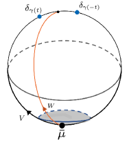
Figure 1. Fluctuation of a non-amenable mean in an unexpected direction

Despite this fluctuation being in an unexpected direction, the fluctuation does not exit the hull, since the measure $\mu$ is supported in a full (albeit small) neighborhood of the south pole.

3.2. Immured measures

A point mass added to a measure $\mu$ can cause the Fréchet mean to escape from ${\bar{\mu}}$ in directions that $\mu$ is unable to predict if the added mass lies outside the support of $\mu$. In contrast, the CLT only concerns perturbations of $\mu$ by masses sampled from $\mu$. It is reasonable to demand that Fréchet means of such samples land, after taking logarithm at ${\bar{\mu}}$, in the convex cone generated by the support.

Definition 3.9 (Immured).

A measure $\mu$ on a smoothly stratified metric space $\mathcal{M}$ is immured if the Fréchet mean ${\bar{\mu}}$ has an open neighborhood $U\subseteq\mathcal{M}$ such that $\log_{\bar{\mu}}{\bar{\mu}}_{n}\in\nolinebreak\operatorname{hull}\mu$ whenever $\mu_{n}$ is a finitely supported measure on $\operatorname{supp}\mu$ and ${\bar{\mu}}_{n}\in U$.

Example 3.10.

Every measure on a $\operatorname{CAT}(0)$ cone is immured, since the log map is an isometry there and the Fréchet mean of any measure on any $\operatorname{CAT}(0)$ space (conical or otherwise) is a limit of points in convex hulls of finite subsets of the support [Stu03, Theorem 4.7]. In particular, every measure on an open book [HHL⁺13] or a phylogenetic tree space as in [BHV01] is immured.

Example 3.11.

A measure $\mu$ on any smoothly stratified metric space $\mathcal{M}$ is immured if the support of $\mu$ contains a neighborhood of its Fréchet mean ${\bar{\mu}}$, because then $\operatorname{hull}\mu=T_{\bar{\mu}}\mathcal{M}$. More generally, $\mu$ is immured if its support is locally convex near ${\bar{\mu}}$ in the sense that $B({\bar{\mu}},\varepsilon)\cap\operatorname{supp}\mu$ is convex in the ball $B({\bar{\mu}},\varepsilon)$ of radius $\varepsilon$ around ${\bar{\mu}}$ for some $\varepsilon>0$.

Example 3.12.

Suppose that $\mu$ is a measure supported on the spine of an open book [HHL⁺13, Theorem 2.9]. Perturbing $\mu$ by adding a mass on a single page of the open book nudges the Fréchet mean ${\bar{\mu}}$ onto that page. Hence the escape cone $E_{\mu}$ equals the entire open book. Limit log along any individual page therefore collapses $E_{\mu}$ non-injectively. This elementary example explains why it is vital to control potential fluctuations by immuring them within the convex hull of the support of the measure (Lemma 4.40 and Corollary 4.42) in addition to their automatic confinement to $E_{\mu}$ (Theorem 4.37).

Remark 3.13.

The immured condition becomes relevant at the very end of Section 4.4.3, specifically Lemma 4.40 on the way to Corollary 4.42, where it confines escape vectors to the fluctuating cone $C_{\mu}$. No result before then, including the rest of Section 4.4.3 through Theorem 4.37, invokes the immured hypothesis. It is possible the immured condition is not necessary at all, for any of the main results; see Remark 4.43.

4. Escape vectors and confinement

Perturbing the measure $\mu$ by adding a small point mass at $x\in\mathcal{M}$ causes the Fréchet mean to escape from the population mean in a deterministic way, as a function of $x$ (Definition 4.1). The central limit theorem can be expressed as identifying the distribution that results when the point $x$ is a random tangent vector generating a Gaussian random tangent field (Theorem 6.14 via Theorem 6.12). The connection to classical expressions of the CLT as identifying the limiting distribution of rescaled Fréchet means of samples from $\mu$ proceeds by directly comparing those means to perturbations along empirical random tangent fields (Proposition 4.24), which suffices by the CLT for random tangent fields (Theorem 2.22).

The reduction of the CLT to empirical tangent perturbation occupies Section 4.2, after introducing concepts surrounding escape vectors in Section 4.1. The empirical perturbation itself is naturally expressed as a minimization over $\mathcal{M}$ or, by taking logarithms, over the tangent cone $T_{\bar{\mu}}\mathcal{M}$ at the Fréchet mean. That minimization is difficult to analyze directly. However, as Section 4.3 shows via well chosen approximations of the problem, it becomes tractable—with explicit formulas and straightforward uniqueness—when the minimization is taken only over the escape cone $E_{\mu}$. This tack succeeds because perturbation of $\mu$ naturally causes the Fréchet mean to exit from ${\bar{\mu}}$ along an escape vector. Confinement to $E_{\mu}$ in this manner is the main result of Section 4, Theorem 4.37. It is particularly potent for central limit theorems when the perturbation of $\mu$ occurs in the support of $\mu$, in which case the escape is further confined to the fluctuating cone $C_{\mu}$ (Corollary 4.42). A functional version of fluctuating confinement in Section 5 relates convergence in the context of escape vectors to convergence in the context of random tangent fields from Section 2.3, which is needed for an application of the continuous mapping theorem to the random field CLT from Theorem 2.22; see Remark 4.38.

The setting throughout Section 4 is that of Definition 2.21, except that $\mathcal{M}$ is not merely $\operatorname{CAT}(\kappa)$ but a smoothly stratified metric space: $x_{1},x_{2},\ldots\!\sim\mu$ are $\mathcal{M}$-valued independent random variables with distribution $\mu$ and empirical measure $\mu_{n}=\frac{1}{n}\sum_{i=1}^{n}\delta_{x_{i}}$, whose Fréchet function

$$F_{n}=F_{\mu_{n}}=\frac{1}{n}\sum_{j=1}^{n}\rho_{x_{j}}$$

is expressed compactly using the half square-distance function $\rho$ from Definition 3.2.

The measure $\mu$ is repeatedly (but not always) required to be amenable throughout this section because of Lemma 4.14 and its heavily cited consequence, Proposition 4.24. That said, many of the definitions make sense for measures that need not be amenable.

In this section, the subscript ${\bar{\mu}}$ is often suppressed in the inner product $\langle Y,Z\rangle_{\bar{\mu}}$ from Definition 2.3 when there is no ambiguity about the identity of the base point.

4.1. Escape vectors

The main result of this section, Theorem 4.37, shows that the output of the following definition exists and is well defined.

Definition 4.1.

Let $\mu$ be a measure on a smoothly stratified metric space $\mathcal{M}$. Fix $x\in\mathcal{M}$ with unit measure $\delta_{x}$ supported at $x$. For positive $t\to 0$, the perturbed measures $\mu+t\delta_{x}$ have Fréchet means ${\overline{\mu+t\delta_{x}}}$.

1. The escape vector of $x$ is

   $$\mathscr{E}(x)=\lim_{t\to 0^{+}}\frac{1}{t}\log_{\bar{\mu}}(\,{\overline{\mu+t\delta_{x}}}\,).$$

2. If $X\in T_{\bar{\mu}}\mathcal{M}$ is a tangent vector with exponential $x=\exp_{\bar{\mu}}X\in\mathcal{M}$, then the escape vector of $X$ is $\mathscr{E}(X)=\mathscr{E}(x)$.

3. More generally, if $X\in T_{\bar{\mu}}\mathcal{M}$ is any tangent vector, then set $\mathscr{E}(X)=\frac{1}{r}\mathscr{E}(rX)$ for any $r>0$ such that $rX$ is exponentiable (cf. Definition 2.12.2).

Remark 4.2.

It is not obvious that the limit in Definition 4.1.1 exists. Indeed, existence is part of the main result of this section, Theorem 4.37, whose primary conclusion is that escape vectors of arbitrary points in $\mathcal{M}$ lie in the escape cone $E_{\mu}$ from Definition 2.9; that is, escape vectors of arbitrary points yield vanishing directional derivatives of the Fréchet function. But arbitrary escape vectors can pull the Fréchet mean out of the fluctuating cone $C_{\mu}$ from Definition 2.11, necessitating Corollary 4.42 for escape vectors of samples from $\mu$.

Remark 4.3.

It is also not obvious that the rescaling procedure in Definition 4.1.3 yields a well defined output. That is also part of Theorem 4.37, the crucial point being homogeneity in Corollary 4.36, which is a consequence of the explicit formula for the radial polar coordinate of the escape vector in terms of its direction Proposition 4.34.

Remark 4.4.

The (limiting distribution in the) CLT can be thought of as resulting from taking Fréchet means after perturbing $\mu$ by adding mass at a single point along a Gaussian random tangent field; indeed, that is the meaning of Theorem 6.14. However, nonlinearity of the tangent cone at ${\bar{\mu}}$ forces consideration of perturbations by mass at finitely many points of $\mathcal{M}$. These finitely many points—or, more precisely, their logarithms in $T_{\bar{\mu}}\mathcal{M}$—are pushed to a vector space $\mathbb{R}^{m}$ by tangential collapse $\mathcal{L}$ (Section 2.2, especially Definition 2.13 and Theorem 2.14), where they are subsequently averaged to get a single vector. The technical obstacle is that this average vector in $\mathbb{R}^{m}$ need not have a preimage in $T_{\bar{\mu}}\mathcal{M}$, such as when $\mathcal{M}$ is the plane $\mathbb{R}^{2}$ with an open quadrant deleted, in which case $\mathcal{L}$ is the inclusion $\mathcal{M}\hookrightarrow\mathbb{R}^{2}$. Definition 4.9 accounts for the fact that assigning an escape vector to this single average vector in $\mathbb{R}^{m}$ (Definition 6.19) is a process that occurs not in $\mathbb{R}^{m}$ but in $T_{\bar{\mu}}\mathcal{M}$, before the vectors can be averaged, by working with finitely supported measures instead of with individual points. Stating Definition 4.9 therefore first requires extensions of inner products (Definition 2.3) and tangent cone rescaling to the setting of discrete measures instead of individual vectors.

Definition 4.5.

A measure $\delta$ on a space $\mathcal{M}$ is sampled from $\mathcal{M}$, written $\delta\Subset\mathcal{M}$, if it has finite support, so for some points $y^{1},\dots,y^{j}\in\mathcal{M}$ it has the form

$$\delta=\lambda_{1}\delta_{y^{1}}+\dots+\lambda_{j}\delta_{y^{j}}.$$

In terms of half square-distance $\rho$ in Definition 3.2, the measure $\delta$ has Fréchet function

$$F_{\delta} =\frac{1}{2}\bigl{(}\lambda_{1}\mathbf{d}^{2}(y^{1},\mathord{\,\cdot\,})+\dots+\lambda_{j}\mathbf{d}^{2}(y^{j},\mathord{\,\cdot\,})\bigr{)}$$

$$=\lambda_{1}\rho_{y^{1}}+\dots+\lambda_{j}\rho_{y^{j}}.$$

Definition 4.6.

For any measure $\Delta=\lambda_{1}\delta_{Y^{1}}+\dots+\lambda_{j}\delta_{Y^{j}}$ sampled from $T_{\bar{\mu}}\mathcal{M}$, set

$$\langle\Delta,\,\cdot\,\rangle=\lambda_{1}\langle Y^{1},\,\cdot\,\rangle+\dots+\lambda_{j}\langle Y^{j},\,\cdot\,\rangle$$

in terms of inner products (Definition 2.3). For any measure $\delta$ sampled from $\mathcal{M}$ with pushforward $(\log_{\bar{\mu}})_{\sharp}\delta=\nolinebreak\Delta$, simplify notation by writing $\Delta=\log_{\bar{\mu}}\delta$. If every $Y^{i}\in T_{\bar{\mu}}\mathcal{M}$ can be exponentiated (cf. Definition 2.12.2; note that this need not be the case even if $Y^{i}=\nolinebreak\log_{\bar{\mu}}y^{i}$ for all $i$), then also write $\delta=\exp_{\bar{\mu}}\Delta$ and say that $\Delta$ can be exponentiated.

Remark 4.7.

When the measure $\mu$ is localized, the discrete measure $\delta$ in Definition 4.6 almost surely has well defined logarithm by Definition 2.7. But transmitting information back to $\mathcal{M}$ requires the tangent vectors supporting $\Delta=\nolinebreak\log_{\bar{\mu}}\delta$ to be sufficiently short, cf. Definition 2.12.2. This issue is rectified, thereby allowing arbitrary measures $\Delta$ sampled from $T_{\bar{\mu}}\mathcal{M}$, using homogeneity in the sense of Definition 2.13.4: vectors in the support of $\Delta$ can be shrunk, operated on, and re-stretched (see Corollary 4.36). However, the default notation $t\Delta$ for $t\geq 0$ has (and needs to have, for the purpose of writing ${\widehat{\mu}}+t\Delta$) the standard meaning

$$t\Delta=t\lambda_{1}\delta_{Y^{1}}+\dots+t\lambda_{j}\delta_{Y^{j}}$$

which necessitates different notation for rescaling the vectors $Y^{1},\dots,Y^{j}$. Placing the scalar after $\Delta$ indicates it should scale the vectors instead of their masses, as follows.

Definition 4.8.

For $\Delta=\lambda_{1}\delta_{Y^{1}}+\dots+\lambda_{j}\delta_{Y^{j}}$ sampled from $T_{\bar{\mu}}\mathcal{M}$ and real $r\geq 0$, set

$$\Delta r=\lambda_{1}\delta_{rY^{1}}+\dots+\lambda_{j}\delta_{rY^{j}}$$

Definition 4.9 (Escape vector).

Fix a measure $\mu$ on a smoothly stratified space $\mathcal{M}$.

1. Any measure $\delta\Subset\mathcal{M}$ has escape vector

   $$\mathscr{E}(\delta)=\lim_{t\to 0^{+}}\frac{1}{t}\log_{\bar{\mu}}(\,{\overline{\mu+t\delta}}\,).$$

2. If $\Delta\Subset T_{\bar{\mu}}\mathcal{M}$ with exponential $\delta=\exp_{\bar{\mu}}\Delta\Subset\mathcal{M}$, then the escape vector of $\Delta$ is $\mathscr{E}(\Delta)=\mathscr{E}(\delta)$.

3. More generally, for any measure $\Delta\Subset T_{\bar{\mu}}\mathcal{M}$, set $\mathscr{E}(\Delta)=\frac{1}{r}\mathscr{E}(\Delta r)$ for any $r>0$ such that $\Delta r$ is exponentiable (cf. Definitions 2.12.2 and 4.8).

The goal of Section 4 is to show in Theorem 4.37 that escape vectors are well defined and moreover can be obtained by minimizing over meaningfully smaller subsets of points or tangent vectors than $\mathcal{M}$ or $T_{\bar{\mu}}\mathcal{M}$. Some further remarks and notations help set the stage for the constructions and proofs in the remainder of Section 4.

Remark 4.10.

The fact that the measure $\mu+t\delta$ is not a probability measure, because the mass of $\delta\Subset\mathcal{M}$ is unrestricted, makes no material difference to Definition 4.1.1 or Definition 4.9.1 because the Fréchet function in Eq. (1.3) is defined just as well for measures of nonunit mass, and the Fréchet mean in Eq. (1.4) is unaffected by globally scaling the measure. Thus the measure $\mu+t\delta$ yields the same minimizer as the probability measure obtained by rescaling $\mu+t\delta$. Geometrically, it can be helpful to think of the Fréchet function $F_{\delta}$ here as extending the notion of half square-distance $\rho$ from Definition 3.2.

Passing from minimization over points in $\mathcal{M}$ to minimization over their logarithms only works reversibly in a neighborhood of ${\bar{\mu}}$, cf. Definition 2.12.2. To maintain precision in the many minimizations to come, it is useful to have notations for sets of exponentiable tangent vectors at ${\bar{\mu}}$.

Definition 4.11.

Given a measure $\mu$ on a smoothly stratified metric space $\mathcal{M}$, let

$$T^{\hskip 0.3014pte}_{\bar{\mu}}\mathcal{M}\subseteq T_{\bar{\mu}}\mathcal{M}\qquad E_{\mu}^{\hskip 0.3014pte}\subseteq E_{\mu}\qquad\text{and}\qquad C_{\mu}^{\hskip 0.1507pte}\subseteq C_{\mu}$$

be the subsets of the tangent cone (Proposition 2.1), escape cone (Definition 2.9), and fluctuating cone (Definition 2.11) consisting of vectors that can be exponentiated.

Remark 4.12.

The $\operatorname*{argmin}$ in Remark 4.10 equals

$$a(t,\delta)=\operatorname*{argmin}_{X\in T^{\hskip 0.21529pte}_{\bar{\mu}}\mathcal{M}}\bigl{(}F(\exp_{\bar{\mu}}X)+tF_{\delta}(\exp_{\bar{\mu}}X)\bigr{)}$$

as long as the deformation of $\mu$ by $t\delta$ is sufficiently mild, so the Fréchet mean doesn’t move too much (see Lemma 4.31). That poses no meaningful obstacle for the purpose of escape vectors, since the point is to take limits as $t\to 0$ anyway.

Remark 4.13.

Rephrasing the $\operatorname*{argmin}$ as taking place over tangent vectors in Remark 4.12 instead of points from $\mathcal{M}$ in Remark 4.10 makes way for alternate methods to recover deformed Fréchet means directly in terms of operations on tangent vectors, notably inner products as in Definition 4.6. The methods use expressions of the form

$$b(t,\Delta) \in\operatorname*{argmin}_{X\in T^{\hskip 0.21529pte}_{\bar{\mu}}\mathcal{M}}\bigl{(}F(\exp_{\bar{\mu}}X)-t\langle\Delta,X\rangle\bigr{)}$$

or, via polar coordinates (Definition 3.3) and the second-order coefficient $$\Lambda_{\bar{\mu}}$$ in the Fréchet function Taylor expansion (Proposition 3.5),

$$c(t,\Delta) \in\operatorname*{argmin}_{X\in T^{\hskip 0.21529pte}_{\bar{\mu}}\mathcal{M}}\bigl{(}r_{X}^{2}\Lambda_{\bar{\mu}}(\theta_{X})-t\langle\Delta,X\rangle\bigr{)}.$$

4.2. Transforming the CLT to a perturbation problem

The goal of this subsection is to transform the problem of finding (the distribution of) the empirical Fréchet mean ${\bar{\mu}}_{n}=\operatorname*{argmin}_{x\in\mathcal{M}}F_{n}(x)$ into the problem of finding the minimizer a function obtained from perturbation of the Fréchet function $F=F_{\mu}$ by the empirical random tangent field ${\overline{g}}_{n}$ from Definition 2.21. This goal is accomplished in Proposition 4.24, which shows that a minimizer

$$h_{n}\in\operatorname*{argmin}_{x\in\mathcal{M}}\bigl{(}F(x)-{\overline{g}}_{n}(\log_{\bar{\mu}}x)\bigr{)}$$

serves as a suitable proxy for the Fréchet mean, in the sense that $\sqrt{n}\,\mathbf{d}(h_{n},{\bar{\mu}}_{n})\xrightarrow{P}0$. Note that ${\overline{g}}_{n}$ is considered here as a random tangent field on $T_{\bar{\mu}}\mathcal{M}$, as in Remark 2.18.

The first step is a uniform law of large numbers. This lemma uses amenability of the measure $\mu$ (Definition 3.2) explicitly in the proof and is one of the reasons for requiring that basic hypothesis. To understand the statement, observe that the quantity $\zeta_{n}$ defined there is a certain proxy, constructed from the law of cosines, for a $\sqrt{n}$-zoomed-in version of the half square-distance from the Fréchet mean ${\bar{\mu}}$ to $z$.

Lemma 4.14.

Fix an amenable measure $\mu$ on a smoothly stratified metric space $\mathcal{M}$. Using the half square-distance function $\rho_{w}$ from Definition 3.2, let

$$\zeta_{n}:\mathcal{M}\times\mathcal{M} \to\mathbb{R}$$

$$(w,z) \mapsto\sqrt{n}\bigl{(}\rho_{w}(z/\sqrt{n})-\rho_{w}({\bar{\mu}})+\langle W,Z/\sqrt{n}\rangle\bigr{)},$$

where $Z/\sqrt{n}=n^{-1/2}\log_{\bar{\mu}}z$ and $z/\sqrt{n}$ is shorthand for $\exp_{\bar{\mu}}(Z/\sqrt{n})$ and $W=\log_{\bar{\mu}}w$. Then for any compact set $U\subseteq\mathcal{M}$ there is a uniform law of large numbers

$$\sup_{z\in U}\Bigl{(}\frac{1}{n}\sum_{i=1}^{n}\sqrt{n}\,\zeta_{n}(x_{i},z/\sqrt{n})-\mathbb{E}\bigl{[}\sqrt{n}\,\zeta_{n}(x,z/\sqrt{n})\bigr{]}\Bigr{)}\xrightarrow{P}0.$$

Proof.

The result essentially follows from a relatively classical uniform law of large numbers (cf. [NM94, Lemma 2.4] or [Jen69]) whose assumptions are that there exists an integrable, positive, measurable function $\mathfrak{f}$ with $|\sqrt{n}\,\zeta_{n}(w,z/\sqrt{n})|\leq C\mathfrak{f}(w)$ for all $z\in U$ and that the family of random variables $\sqrt{n}\,\zeta_{n}(w,z/\sqrt{n})$ is uniformly continuous in $z$ in a sense made precise below. The argument is sketched here assuming existence of such a function $\mathfrak{f}$ and the needed uniform continuity.

The weak law of large numbers for triangular arrays (see [Dur19, Theorem 2.2.6] with $b_{n}=\sqrt{n}$) implies that for any fixed $z$,

$$\frac{1}{n}\sum_{i=1}^{n}\sqrt{n}\,\zeta_{n}(x_{i},z/\sqrt{n})-\mathbb{E}\sqrt{n}\,\zeta_{n}(x,z/\sqrt{n})\rightarrow 0$$

in probability as $n\rightarrow\infty$.

Since $U$ is compact and $\frac{\partial}{\partial z}\bigl{(}\sqrt{n}\,\zeta_{n}(w,z/\sqrt{n})\bigr{)}=\frac{\partial\zeta_{n}}{\partial z}(w,z/\sqrt{n})$, the collection of functions $\bigl{\{}\sqrt{n}\,\zeta_{n}(w,z/\sqrt{n})\bigm{|}n\in\mathbb{N}\bigr{\}}$ is uniformly continuous in $z$. From this and the discussion below, there also exists an integrable, positive measurable $\mathfrak{g}(w)$ so that for all $z\in U$ and $n\in\mathbb{N}$, and for all $\varepsilon>0$,

$$\gamma(z,w,\varepsilon):=\sup_{z^{\prime}\in B(z,\delta)}\bigl{|}\sqrt{n}\zeta_{n}(w,z^{\prime}/\sqrt{n})-\sqrt{n}\zeta_{n}(w,z/\sqrt{n})\bigr{|}\leq\mathfrak{g}(w)\varepsilon.$$

Fixing any $\varepsilon>0$, let $\{z_{k}\mid k=1,\dots,K_{\varepsilon}\}\subset U$ be such that $U\subset\bigcup_{k}B(z_{k},\varepsilon)$. Then

$$\sup_{z\in U} \Bigl{(}\frac{1}{n}\sum_{i=1}^{n}\sqrt{n}\,\zeta_{n}(x_{i},z/\sqrt{n})-\mathbb{E}\bigl{[}\sqrt{n}\,\zeta_{n}(x,z/\sqrt{n})\bigr{]}\Bigl{)}$$

$$=\max_{k\in\{1,\dots,K_{\varepsilon}\}}\sup_{z\in B(z_{k},\varepsilon)}\Bigl{(}\frac{1}{n}\sum_{i=1}^{n}\sqrt{n}\,\zeta_{n}(x_{i},z/\sqrt{n})-\mathbb{E}\bigl{[}\sqrt{n}\,\zeta_{n}(x,z/\sqrt{n})\bigr{]}\Bigr{)}$$

$$\leq\sup_{k\in\{1,\dots,K_{\varepsilon}\}}\Bigl{(}\frac{1}{n}\sum_{i=1}^{n}\sqrt{n}\,\zeta_{n}(x_{i},z_{k}/\sqrt{n})-\mathbb{E}\bigl{[}\sqrt{n}\,\zeta_{n}(x,z_{k}/\sqrt{n})\bigr{]}\Bigr{)}+\frac{\varepsilon}{n}\sum_{j=1}^{n}\mathfrak{g}(x_{j}).$$

The first term (with the supremum over $k$) goes to zero for each $\varepsilon$ by the weak law of large numbers. Again by the weak law of large numbers, the second term is bounded in probability by a constant times $\varepsilon$ as $n\rightarrow\infty$. Since $\varepsilon$ is arbitrary the proof is complete except for showing the existence of $\mathfrak{f}$ and $\mathfrak{g}$. Details are provided for the first, as the second is similar.

Suppose that $w$ and $z$ are two points in $\mathcal{M}$. Let

$$\gamma_{n}(t)=\exp_{\bar{\mu}}t\frac{Z}{\|Z\|}\text{ for }t\in\bigl{[}0,\|Z\|/\sqrt{n}\,\bigr{]}$$

be the unit speed geodesic from ${\bar{\mu}}$ to $z/\sqrt{n}$ and $Y_{n}(t)=\log_{\bar{\mu}}\gamma_{n}(t)$. Then the Taylor expansion at ${\bar{\mu}}$ of the half square-distance function $\rho_{w}$ evaluated at $z/\sqrt{n}$ reads

$$\rho_{w}(z/\sqrt{n})=\rho_{w}({\bar{\mu}})-\langle\log_{\bar{\mu}}w,Z/\sqrt{n}\rangle_{\bar{\mu}}+\frac{1}{2}\|Y_{n}(t_{0})\|^{2}\lambda_{w}\bigl{(}Y_{n}(t_{0})/t_{0}\bigr{)}$$

for some $t_{0}\in\bigl{[}0,\|Z\|/\sqrt{n}\,\bigr{]}$ by the Lagrange form of the remainder, where the middle term on the right is because $\nabla_{{\bar{\mu}}}\rho_{w}(V)=-\langle\log_{\bar{\mu}}w,V\rangle$ for all $V\in T_{\bar{\mu}}\mathcal{M}$ (this is [MMT23b, Proposition 2.5]) and the $\lambda_{w}$ term is as in Definition 3.2. Rearranging yields

(4.1) $$\rho_{w}(z/\sqrt{n})-\rho_{w}({\bar{\mu}})+\langle\log_{\bar{\mu}}w,Z/\sqrt{n}\rangle_{\bar{\mu}}=\frac{1}{2}\|Y_{n}(t_{0})\|^{2}\lambda_{w}\bigl{(}Y_{n}(t_{0})/t_{0}\bigr{)}.$$

Because $\|Y_{n}(t)\|=t\leq\|Z\|/\sqrt{n}$, there is a universal constant $C>0$ such that

$$\|Y_{n}(t)\|<\sqrt{2}n^{-1/2}C\text{ for all }z\in U\text{ and }t\in\bigl{[}0,\|Z\|/\sqrt{n}\,\bigr{]}.$$

By amenability (Definition 3.2) the second-order directional derivative $\lambda_{w}\bigl{(}Z/\|Z\|\bigr{)}$ of $\rho_{x}$ is dominated by a $\mu$-integrable function $\mathfrak{f}(w)$. Thus (4.1) implies

$$|\rho_{w}(z/\sqrt{n})-\rho_{w}({\bar{\mu}})+\langle\log_{\bar{\mu}}w,Z/\sqrt{n}\rangle_{\bar{\mu}}| \leq\frac{1}{2}(\sqrt{2}n^{-1/2}C)^{2}\mathfrak{f}(w)$$

$$\leq n^{-1}C^{2}\mathfrak{f}(w)$$

for all $z\in U$. Therefore, for all $z\in U$,

$$\bigl{|}\zeta_{n}(w,z/\sqrt{n})\bigr{|} =\bigl{|}\sqrt{n}\,\bigl{(}\rho_{w}(z/\sqrt{n})-\rho_{w}({\bar{\mu}})+\langle\log_{\bar{\mu}}w,Z/\sqrt{n}\rangle_{\bar{\mu}}\bigr{)}\bigr{|}$$

$$\leq n^{-1}C^{2}\mathfrak{f}(w),$$

which implies that

$$\bigl{|}\sqrt{n}\,\zeta_{n}(w,z/\sqrt{n})\bigr{|}\leq C^{2}\mathfrak{f}(w),$$

completing the proof. ∎

It is also necessary to recall a law of large numbers for the empirical means ${\bar{\mu}}_{n}$. This result does not require the measure $\mu$ to be amenable.

Theorem 4.15.

For any measure $\mu$ on a smoothly stratified metric space $\mathcal{M}$,

$$\lim_{n\to\infty}\mathbf{d}({\bar{\mu}}_{n},{\bar{\mu}})\overset{P}{=}0.$$

Proof.

See [Stu03] for $\operatorname{CAT}(0)$ spaces and [Yok16] for $\operatorname{CAT}(\kappa)$ with $\kappa>0$. ∎

The following result is used in the proof that $\sqrt{n}\log_{\bar{\mu}}{\bar{\mu}}_{n}$ is tight (Proposition 4.19).

Lemma 4.16 ([Van00, Theorem 5.52]).

Let $C$ be a constant and $\alpha>\beta$ be positive integers. Assume that for every $n$ and sufficiently small $\delta>0$, the Fréchet function $F=\nolinebreak F_{\mu}$ and the empirical Fréchet function $F_{n}=F_{\mu_{n}}$ satisfy

(4.2) $$\sup_{\mathbf{d}(z,{\bar{\mu}})<\delta}\bigl{|}F(x)-F({\bar{\mu}})\bigr{|}\geq C\delta^{\alpha}$$

(4.3) $$\makebox[0.0pt][r]{and\quad\ }\mathbb{E}\Bigl{[}\sqrt{n}\sup_{z\in B({\bar{\mu}},\delta)}\bigl{(}F_{n}(z)-F(z)-F_{n}({\bar{\mu}})+F\bigl{(}{\bar{\mu}})\bigr{)}\Bigr{]}\leq C\delta^{\beta}.$$

If additionally $\mathbf{d}({\bar{\mu}}_{n},{\bar{\mu}})\xrightarrow{P}0$ then $n^{1/(2\alpha-2\beta)}\mathbf{d}({\bar{\mu}}_{n},{\bar{\mu}})$ is tight.

Proof.

The proof is adapted from [Van00, Theorem 5.52] to our setting with some simplifications particular to our setting. For notational brevity, set the scale $r_{n}=n^{\frac{1}{2\alpha-2\beta}}$.

For each integer $n$ and $\varepsilon>0$, define

$$S_{j,n}^{\varepsilon}=\{z\in\mathcal{M}\mid 2^{j-1}<r_{n}\mathbf{d}(z,{\bar{\mu}})\leq 2^{j},\mathbf{d}(z,{\bar{\mu}})<\varepsilon\}.$$

Observe that the event $\{r_{n}\mathbf{d}({\bar{\mu}}_{n},{\bar{\mu}})>2^{M},\mathbf{d}({\bar{\mu}},{\bar{\mu}})<\varepsilon\}$ coincides with $\bigcup_{j\geq M}\{{\bar{\mu}}_{n}\!\in\nolinebreak\!S_{j,n}^{\varepsilon}\}$. Let $\delta$ be as in (4.2) and observe that fixing any $\varepsilon<\delta$, (4.2) guarantees that

$$z\in S_{j,n}^{\varepsilon}\Rightarrow F({\bar{\mu}})-F({\bar{\mu}}_{n})\leq-C\frac{2^{(j-1)\alpha}}{r_{n}^{\alpha}}\,.$$

Combining this implication with the fact that $F_{n}({\bar{\mu}}_{n})-F_{n}({\bar{\mu}})\leq 0$ almost surely, since ${\bar{\mu}}_{n}$ almost surely minimises $F_{n}$, produces

$$\{{\bar{\mu}}_{n}\in S_{j,n}^{\varepsilon}\} =\bigl{\{}F({\bar{\mu}})-F({\bar{\mu}}_{n})\leq-C\tfrac{2^{(j-1)\alpha}}{r_{n}^{\alpha}}\bigr{\}}\cap\bigl{\{}{\bar{\mu}}_{n}\in S_{j,n}^{\varepsilon}\bigr{\}}$$

$$=\bigl{\{}F({\bar{\mu}})-F({\bar{\mu}}_{n})+F_{n}({\bar{\mu}}_{n})-F_{n}({\bar{\mu}})\leq-C\tfrac{2^{(j-1)\alpha}}{r_{n}^{\alpha}}\bigr{\}}\cap\bigl{\{}{\bar{\mu}}_{n}\in S_{j,n}^{\varepsilon}\bigr{\}}$$

$$\subseteq\Bigl{\{}\sup_{z\in\mathcal{M}\,\mid\,\mathbf{d}(z,{\bar{\mu}})<2^{j}/r_{n}}n^{\frac{1}{2}}|F_{n}(z)-F(z)+F({\bar{\mu}})-F_{n}({\bar{\mu}})|\geq C\tfrac{n^{\frac{1}{2}}2^{(j-1)\alpha}}{r_{n}^{\alpha}}\Bigr{\}}.$$

Applying (4.3) and Markov’s inequality to the last term on the right above produces for $n$ sufficiently large

$$\mathbf{P}\bigl{(}\{r_{n}\mathbf{d}({\bar{\mu}}_{n},{\bar{\mu}})>2^{M}\}\cap\{\mathbf{d}({\bar{\mu}}_{n},{\bar{\mu}})<\varepsilon\}\bigr{)} =\sum_{j\geq M}\mathbf{P}\{{\bar{\mu}}_{n}\in S_{j,n}^{\varepsilon}\}$$

$$\leq\frac{r_{n}^{\alpha-\beta}}{n^{\frac{1}{2}}}\sum_{j\geq M}\frac{C}{2^{j(\alpha-\beta)}}\leq C_{\alpha,\beta,\varepsilon}2^{-M(\alpha-\beta)}$$

for some positive constant $C_{\alpha,\beta,\varepsilon}$ which depends on $\alpha$, $\beta$, and $\varepsilon$ but not on $n$ or $M$. Using this conclusion, observe that

$$\mathbf{P}\bigl{(}\{r_{n}\mathbf{d}({\bar{\mu}}_{n},{\bar{\mu}})>2^{M}\}\bigr{)}= \ \mathbf{P}\bigl{(}\{r_{n}\mathbf{d}({\bar{\mu}}_{n},{\bar{\mu}})>2^{M}\}\cap\{\mathbf{d}({\bar{\mu}}_{n},{\bar{\mu}})<\varepsilon\}\bigr{)}$$

$$\qquad+\mathbf{P}\bigl{(}\{r_{n}\mathbf{d}({\bar{\mu}}_{n},{\bar{\mu}})>2^{M}\}\cap\{\mathbf{d}({\bar{\mu}}_{n},{\bar{\mu}})\geq\varepsilon\}\bigr{)}$$

$$\leq \ C_{\alpha,\beta,\varepsilon}2^{-M(\alpha-\beta)}+\mathbf{P}\bigl{(}\mathbf{d}({\bar{\mu}}_{n},{\bar{\mu}})\geq\varepsilon\bigr{)}.$$

Since $\mathbf{d}({\bar{\mu}}_{n},{\bar{\mu}})\rightarrow 0$ in probability the last term goes to $0$ for all $\varepsilon>0$ as $n\rightarrow\infty$. ∎

Lemma 4.17.

Assume that $\mu$ is a probability measure such that $\int_{\mathcal{M}}d^{2}(x,{\bar{\mu}})\mu(dx)\leq K<\infty$. Then for any sufficiently small $\delta>0$ and any $n\in\mathbb{N}$,

$$\mathbb{E}\Bigl{[}\sqrt{n}\sup_{z\in B({\bar{\mu}},\delta)}\bigl{|}F_{n}(z)-F(z)+F({\bar{\mu}})-F_{n}({\bar{\mu}})\bigr{|}\Bigr{]} \leq C\delta,$$

where the constant $C$ does not depend on $\delta$.

Proof.

The proof is essentially the same as the proof of [Van00, Corollary 5.53]. There they employ [Van00, Lemma 19.34 and Corollary 19.35] to obtain the result via a chaining argument. The proof in [Van00, Corolary 5.53] is written in Euclidian space, but the results in [Van00, Lemma 19.34 and Corollary 19.35] are written for a general measure space. There are two facts in our setting which are needed to apply the result. First, in the notation of [Van00, Lemma 19.34, Corollary 19.35, and Example 19.7], it needs to be shown that $|\mathbf{d}^{2}(w_{1},z)-\mathbf{d}^{2}(w_{2},z)|\leq\dot{m}(z)\mathbf{d}(w_{1},w_{2})$ for all $w_{1},w_{2}\in B({\bar{\mu}},\delta)$ for $\delta$ sufficiently small and that $\int\dot{m}(z)^{2}\mu(dz)\leq\infty$. Observe that for $w_{1},w_{2}\in B({\bar{\mu}},\delta)$,

$$|\mathbf{d}^{2}(w_{1},z)-\mathbf{d}^{2}(w_{2},z)| =\lvert\mathbf{d}(w_{1},z)+\mathbf{d}(w_{2},z)\rvert\lvert\mathbf{d}(w_{1},z)-\mathbf{d}(w_{2},z)\rvert$$

$$\leq\bigl{(}\mathbf{d}(w_{1},z)+\mathbf{d}(w_{2},z)\bigr{)}\mathbf{d}(w_{1},w_{2})$$

$$\leq 2\bigl{(}\mathbf{d}({\bar{\mu}},z)+\delta\bigr{)}\mathbf{d}(w_{1},w_{2}).$$

So for $\delta$ sufficiently small, take $\dot{m}(z)=2\mathbf{d}({\bar{\mu}},z)+1$. By assumption, $\int\dot{m}(z)^{2}\mu(dz)\leq\nolinebreak\infty$.

The last needed ingredient is the entropy, which captures how log of the $\varepsilon$-covering number scales with $\varepsilon$, as discussed in [MMT23c, Section 3.3, especially Eq. (3.2)]. [Van00, Example 19.7] explains how to demonstrate that $\log(\frac{1}{\varepsilon})$ bounds the entropy in our setting when $z$ is in Euclidian space. Since locally our stratified space is just a union of a countable (in fact, finite) number of smooth manifolds, the result carries over to our setting by adding the log of the covering number of each of the strata. The result still scales like $\log(1/\varepsilon)$. This reasoning is covered in [MMT23c, Lemma 3.6]. ∎

Remark 4.18.

The fact that these chaining proofs can be adapted to our setting is not surprising, as the proofs of [Van00, Lemma 19.34 and Corolary 19.35] are more sophisticated versions of the chaining proof given in detail in [MMT23c, Theorem 3.1 and Lemma 5.8].

Now the tightness of $\sqrt{n}\log_{\bar{\mu}}{\bar{\mu}}_{n}$ can be addressed.

Proposition 4.19.

For any amenable measure $\mu$ on a smoothly stratified metric space, the sequence $\sqrt{n}\mathbf{d}({\bar{\mu}}_{n},{\bar{\mu}})$ is asymptotically bounded in probability as $n\rightarrow\infty$.

Proof.

Apply Lemma 4.16 for $\alpha=2$ and $\beta=1$. The LLN in Theorem 4.15 says that $\mathbf{d}({\bar{\mu}}_{n},{\bar{\mu}})\xrightarrow{P}0$. It remains to check the two inequalities in Lemma 4.16. The second one follows from Lemma 4.17. Next, recall from Lemma 3.6 that there is a universal constant $C$, independent of the measure $\mu$, such that for all $x$ in some neighborhood $B({\bar{\mu}},\delta)$ of ${\bar{\mu}}$ with $\delta<R_{\kappa/2}$,

$$|F(x)-F({\bar{\mu}})|\geq C\mathbf{d}^{2}(x,{\bar{\mu}}).$$

Thus the first inequality in Lemma 4.16 also holds. ∎

Remark 4.20.

The following results, culminating in Proposition 4.24, imply that to determine the limit law for the empirical Fréchet mean ${\bar{\mu}}_{n}$, it suffices to instead minimize the population Fréchet function after it is perturbed radially by an infinitesimal tangent field defined from a finite sample. That is because, in Proposition 4.24, the convergence of $h_{n}$ to ${\bar{\mu}}_{n}$ occurs even after stretching by a factor of $\sqrt{n}$.

Definition 4.21.

Fix a measure $\mu$ on a smoothly stratified space $\mathcal{M}$. The empirical tangent field ${\overline{g}}_{n}$ induced by $\mu$ (Definition 2.21) yields the average sample perturbation

$$h_{n}\in\operatorname*{argmin}_{x\in\mathcal{M}}\bigl{(}F(x)-{\overline{g}}_{n}(\log_{\bar{\mu}}x)\bigr{)},$$

where again ${\overline{g}}_{n}$ is considered a random tangent field on $T_{\bar{\mu}}\mathcal{M}$ via Remark 2.18.

Remark 4.22.

The $\operatorname*{argmin}$ defining an average sample perturbation is a set rather than a point, even when considered deterministically. But the choice of point in that set is irrelevant, since all choices behave the same way for convergence purposes, as follows.

Lemma 4.23.

Any rescaled average sample perturbation $\sqrt{n}\log_{\bar{\mu}}h_{n}$ is tight.

Proof.

First note that $\lim_{n\to\infty}\mathbf{d}({\bar{\mu}},h_{n})=0$. To see why, Lemma 3.6 says that there is a constant $C>0$ satisfying $F(x)-F({\bar{\mu}})\geq C\mathbf{d}^{2}({\bar{\mu}},x)$. On the other hand, because ${\overline{g}}_{n}$ is homogeneous as a random tangent field on $T_{\bar{\mu}}\mathcal{M}$ by Remark 2.18,

$${\overline{g}}_{n}(\log_{\bar{\mu}}x)-{\overline{g}}_{n}(\log_{\bar{\mu}}{\bar{\mu}})={\overline{g}}_{n}(\log_{\bar{\mu}}x)=\mathbf{d}({\bar{\mu}},x){\overline{g}}_{n}\bigl{(}\theta_{x}\bigr{)},$$

where $\theta_{x}$ is the direction of $x$ in polar coordinates (Definition 3.3). Thus

$${\overline{g}}_{n}(\log_{\bar{\mu}}x)-{\overline{g}}_{n}(\log_{\bar{\mu}}{\bar{\mu}})\leq\mathbf{d}({\bar{\mu}},x)\sup_{\theta\in S_{\bar{\mu}}\mathcal{M}}{\overline{g}}_{n}(\theta)=\frac{\mathbf{d}({\bar{\mu}},x)}{\sqrt{n}}\sup_{\theta\in S_{\bar{\mu}}\mathcal{M}}\sqrt{n}\,{\overline{g}}_{n}(\theta).$$

Subtracting this equation from the equation in Lemma 3.6 gives

$$F(x)-{\overline{g}}_{n}(\log_{\bar{\mu}}x)-F({\bar{\mu}})+{\overline{g}}_{n}(\log_{\bar{\mu}}{\bar{\mu}})\geq C\mathbf{d}^{2}({\bar{\mu}},h_{n})-\frac{\mathbf{d}({\bar{\mu}},h_{n})}{\sqrt{n}}\sup_{\theta\in S_{\bar{\mu}}\mathcal{M}}\sqrt{n}\,{\overline{g}}_{n}(\theta).$$

Replacing $x$ by $h_{n}$ and using that $h_{n}$ is a minimizer yields

$$0\geq F(h_{n})-{\overline{g}}_{n}(\log_{\bar{\mu}}h_{n})-F({\bar{\mu}})+{\overline{g}}_{n}(\log_{\bar{\mu}}{\bar{\mu}})\geq C\mathbf{d}^{2}({\bar{\mu}},h_{n})-\frac{\mathbf{d}({\bar{\mu}},h_{n})}{\sqrt{n}}\sup_{\theta\in S_{\bar{\mu}}\mathcal{M}}\sqrt{n}\,{\overline{g}}_{n}(\theta),$$

which implies that

(4.4) $$\frac{\sup_{\theta\in S_{\bar{\mu}}\mathcal{M}}\sqrt{n}\,{\overline{g}}_{n}(\theta)}{C}\geq\sqrt{n}\,\mathbf{d}({\bar{\mu}},h_{n}).$$

[MMT23c, Lemma 5.8] says that $G_{n}=\sqrt{n}\,{\overline{g}}_{n}$ is tight in $\mathcal{C}(S_{\bar{\mu}}\mathcal{M},\mathbb{R})$. In particular, $\sup_{\theta\in S_{\bar{\mu}}\mathcal{M}}\sqrt{n}\,{\overline{g}}_{n}(\theta)$ is tight. Thus (4.4) implies that $\sqrt{n}\,\mathbf{d}(h_{n},{\bar{\mu}})$ is also tight, completing the proof. ∎

Proposition 4.24.

Fix an amenable measure $\mu$ on a smoothly stratified metric space. Any average sample perturbation $h_{n}$ (Definition 4.21) converges in probability to the Fréchet mean faster than $1/\sqrt{n}$:

$$\sqrt{n}\,\mathbf{d}(h_{n},{\bar{\mu}}_{n})\xrightarrow{P}0.$$

Proof.

First expand, using the zoomed-in half square-distances $\zeta_{n}$ from Lemma 4.14:

$$n^{1/2}\Bigl{(}\frac{1}{n}\sum_{i=1}^{n} \zeta_{n}(x_{i},z/\sqrt{n})-\mathbb{E}\bigl{[}\zeta_{n}(x,z/\sqrt{n})\bigr{]}\Bigr{)}$$

(4.5) $$=n\biggl{(}\frac{1}{n}\Bigl{(}\sum_{j=1}^{n}\rho_{x_{j}}(z/\sqrt{n})-\sum_{j=1}^{n}\rho_{x_{j}}({\bar{\mu}})+\sum_{j=1}^{n}\langle X_{j},Z/\sqrt{n}\rangle\Bigr{)}$$

$$\phantom{\mbox{}=n\biggl{(}\biggr{.}}\ \ -\int_{\mathcal{M}}\rho_{x}(z/\sqrt{n})\mu(dx)+\int_{\mathcal{M}}\rho_{x}({\bar{\mu}})\mu(dx)-\int_{\mathcal{M}}\langle X,Z/\sqrt{n}\rangle\mu(dx)\biggr{)}.$$

Noting that $F_{n}(z)=\frac{1}{n}\sum_{j=1}^{n}\rho_{x_{j}}(z)$ and $F(z)=\int_{\mathcal{M}}\rho_{x}(z)\mu(dx)$, Eq. (4.5) reduces to

$$\begin{split}n^{1/2}\Bigl{(}\frac{1}{n}\sum_{i=1}^{n}&\zeta_{n}(x_{i},z/\sqrt{n})-\mathbb{E}\bigl{[}\zeta_{n}(x,z/\sqrt{n})\bigr{]}\Bigr{)}\\ &=n\bigl{(}F_{n}(z/\sqrt{n})-F_{n}({\bar{\mu}})\bigr{)}+nF({\bar{\mu}})-n\bigr{(}F(z/\sqrt{n})-{\overline{g}}_{n}(Z/\sqrt{n})\bigr{)}.\end{split}$$

Lemma 4.14 implies that the left-hand side is a sequence of stochastic processes converging uniformly to $0$ for $z$ in any compact set $U$ around ${\bar{\mu}}$. Hence the equation implies

(4.6) $$\sup_{z\in U}\Bigl{(}n\bigl{(}F_{n}(z/\sqrt{n})-F_{n}({\bar{\mu}})\bigr{)}+nF({\bar{\mu}})-n\bigl{(}F(z/\sqrt{n})-{\overline{g}}_{n}(Z/\sqrt{n})\bigr{)}\Bigr{)}=c_{n},$$

where $c_{n}$ is a random real valued sequence, independent of $z$, converging to $0$ in probability. Thus $z$ can be replaced by any tight random sequence in $\mathcal{M}$. Thanks to Lemma 4.23 and Proposition 4.19, both

$$\sqrt{n}\,{\bar{\mu}}_{n} =\exp(\sqrt{n}\log_{\bar{\mu}}{\bar{\mu}}_{n})$$

$$\text{and\quad}\sqrt{n}\,h_{n} =\exp(\sqrt{n}\log_{\bar{\mu}}h_{n})$$

are valid choices for $z$. Substituting them for $z$ in (4.6) produces

(4.7) $$n\bigl{(}F_{n}(h_{n})-F_{n}({\bar{\mu}})\bigr{)}=-nF({\bar{\mu}})+n\bigl{(}F(h_{n})-{\overline{g}}_{n}(\log_{\bar{\mu}}h_{n})\bigr{)}+c_{n}$$

and

(4.8) $$n\bigl{(}F_{n}({\bar{\mu}}_{n})-F_{n}({\bar{\mu}})\bigr{)}=-nF({\bar{\mu}})+n\bigl{(}F({\bar{\mu}}_{n})-{\overline{g}}_{n}(\log_{\bar{\mu}}{\bar{\mu}}_{n})\bigr{)}+c_{n}.$$

The definition of average sample perturbation $h_{n}$ (Definition 4.21) yields

$$h_{n}\in\operatorname*{argmin}_{x\in\mathcal{M}}\Bigl{(}-nF({\bar{\mu}})+n\bigl{(}F(x)-{\overline{g}}_{n}(\log_{\bar{\mu}}x)\bigr{)}\Bigr{)}.$$

Therefore

$$-nF({\bar{\mu}})+n\bigl{(}F(h_{n})-{\overline{g}}_{n}(\log_{\bar{\mu}}x)\bigr{)}\leq-nF({\bar{\mu}})+n\bigl{(}F({\bar{\mu}}_{n})-{\overline{g}}_{n}(\log_{\bar{\mu}}x)\bigr{)}.$$

Combining this inequality with (4.7) and (4.8) yields

$$n\bigl{(}F_{n}(h_{n})-F_{n}({\bar{\mu}})\bigr{)}-c_{n} =-nF({\bar{\mu}})+n\bigl{(}F(h_{n})-{\overline{g}}_{n}(\log_{\bar{\mu}}x)\bigr{)}$$

$$\leq-nF({\bar{\mu}})+n\bigl{(}F({\bar{\mu}}_{n})-{\overline{g}}_{n}(\log_{\bar{\mu}}x)\bigr{)}$$

$$=n\bigl{(}F_{n}({\bar{\mu}}_{n})-F_{n}({\bar{\mu}})\bigr{)}-c_{n}.$$

In short,

(4.9) $$n\bigl{(}F_{n}(h_{n})-F_{n}({\bar{\mu}})\bigr{)}\leq n\bigl{(}F_{n}({\bar{\mu}}_{n})-F_{n}({\bar{\mu}})\bigr{)}-2c_{n}.$$

On the other hand, ${\bar{\mu}}_{n}=\operatorname*{argmin}_{x\in\mathcal{M}}F_{n}(x)$, so

$${\bar{\mu}}_{n}=\operatorname*{argmin}_{x\in\mathcal{M}}\,n\bigl{(}F_{n}(x)-F_{n}({\bar{\mu}})\bigr{)}.$$

Therefore, for every $n$,

$$n\bigl{(}F_{n}({\bar{\mu}}_{n})-F_{n}({\bar{\mu}})\bigr{)}\leq n\bigl{(}F_{n}(h_{n})-F_{n}({\bar{\mu}})\bigr{)}.$$

From this inequality and (4.9) it follows that

(4.10) $$\bigl{|}n\bigl{(}F_{n}({\bar{\mu}}_{n})-F_{n}(h_{n})\bigr{)}\bigr{|}\leq 2c_{n}.$$

Lemma 3.6 produces a universal constant $C$, independent of the measure $\mu$, such that

$$\bigl{|}F_{n}({\bar{\mu}}_{n})-F_{n}(h_{n})\bigr{|}\geq C\mathbf{d}^{2}({\bar{\mu}}_{n},h_{n})$$

for some positive constant $C$. This inequality, in conjunction with (4.10), yields

$$\mathbf{d}({\bar{\mu}}_{n},h_{n})^{2}\leq\frac{2c_{n}}{nC},$$

or equivalently

$$\sqrt{n}\,\mathbf{d}({\bar{\mu}}_{n},h_{n})\leq\sqrt{\frac{2c_{n}}{C}},$$

which implies the Proposition since $c_{n}\xrightarrow{P}0$ as $n\to\infty$ by (4.6). ∎

4.3. Escape convergence and confinement

Escape vector theory rests on convergence of three flavors sequences that bring uniqueness, homogeneity, duality, an explicit formula, and confinement to the escape cone.

Notation 4.25.

Fix a measure $\mu$ on a smoothly stratified metric space $\mathcal{M}$ and

• a measure $\Delta=\lambda_{1}\delta_{Y^{1}}+\dots+\lambda_{j}\delta_{Y^{j}}$ sampled from $T_{\bar{\mu}}\mathcal{M}$;

• a sequence of measures $\Delta_{n}$ sampled from $T_{\bar{\mu}}\mathcal{M}$ converging weakly to $\Delta$ and

• a sequence of positive real numbers $t_{n}$ converging to $0$.

Using inner products (Definition 2.3), polar coordinates (Definition 3.3), and the second-order Taylor coefficient $\Lambda_{\bar{\mu}}$ of the Fréchet function (Proposition 3.5), define

$$b_{n} \in\operatorname*{argmin}_{x\in\exp_{\bar{\mu}}(E_{\mu}^{\hskip 0.21529pte})}\bigl{(}F(x)-t_{n}\langle\Delta_{n},\log_{\bar{\mu}}x\rangle\bigr{)}$$

$$\text{and}\quad c_{n} \in\operatorname*{argmin}_{x\in\exp_{\bar{\mu}}(E_{\mu}^{\hskip 0.21529pte})}\bigl{(}r_{x}^{2}\Lambda_{\bar{\mu}}(\theta_{x})-t_{n}\langle\Delta_{n},\log_{\bar{\mu}}x\rangle\bigr{)}$$

$$a_{n} =\operatorname*{argmin}_{x\in\exp_{\bar{\mu}}(E_{\mu}^{\hskip 0.21529pte})}\bigl{(}F(x)+t_{n}F_{\delta_{n}}(x)\bigr{)}.$$

Remark 4.26.

For $x\in\exp_{\bar{\mu}}E_{\mu}^{\hskip 0.3014pte}$, the (directional) Taylor expansion of the Fréchet function in Proposition 3.5 becomes

$$F(x)=F({\bar{\mu}})+r_{x}^{2}\Lambda_{\bar{\mu}}(\theta_{x})+o(r_{x}^{2})$$

because $\nabla_{{\bar{\mu}}}F(\theta_{x})=0$. Therefore the function minimized for $b_{n}$ is the function minimized for $c_{n}$ plus a constant and a hyperquadratic term, namely $F({\bar{\mu}})+o(r_{x}^{2})$.

Remark 4.27.

The sequences $b_{n}$ and $c_{n}$ are defined regardless of whether $\Delta_{n}$ is expressible as the logarithm of a measure sampled from $\mathcal{M}$. Of course, $\Delta_{n}$ is always a scalar multiple of such a logarithm, namely $\Delta_{n}=\frac{1}{t}\log_{\bar{\mu}}\exp_{\bar{\mu}}t\Delta_{n}$ for any positive $t\ll 1$ by Definition 2.12.2. The fact that $\Delta$ need not itself be a logarithm becomes irrelevant anyway: by Corollary 4.36, the limiting quantities derived from $a_{n}$, $b_{n}$, and $c_{n}$ are homogeneous—they behave well with respect to scaling $\Delta$ in the sense of Definition 4.8—so $\Delta$ can be shrunk to any desired length for the purpose of comparing $b_{n}$ to $a_{n}$, as long as $\Delta$ is stretched back to its original length later.

Remark 4.28.

That the minimizations in Notation 4.25 are taken over a subset of the escape cone and not all of it also causes no problems because the points $x$ of interest lie arbitrarily close to ${\bar{\mu}}$ for large $n$. Indeed, since $t_{n}\to 0$, the three sequences all minimize small perturbations of the Fréchet function; see Lemma 4.31 for an upper bound.

Remark 4.29.

The goal is to find the limit of $\log_{\bar{\mu}}b_{n}/t_{n}$ as $n\to\infty$ in Theorem 4.37, ideally—if the limit exists—without any dependence on the choice of $b_{n}$ in the $\operatorname*{argmin}$, which is selected from a set and need not be unique (Remark 4.22). The idea is to use $a_{n}$ since it is the (unique) minimizer of a convex function on $\mathcal{M}$ and is also automatically confined to the escape cone $E_{\mu}$ (Proposition 4.32). If $\mathbf{d}(a_{n},{\bar{\mu}})\leq Kt_{n}$ for all $n$ and a finite constant $K$, as is indeed proved in Lemma 4.31, then Taylor expansions of $F_{\delta_{n}}(x)$ and $F(x)$ can be used to approximate $a_{n}$ to order $o(t_{n})$. Consequently, in Proposition 4.34 the limits

$$\lim_{n\to\infty}\frac{\log_{\bar{\mu}}a_{n}}{t_{n}}=\lim_{n\to\infty}\frac{\log_{\bar{\mu}}b_{n}}{t_{n}}=\lim_{n\to\infty}\frac{\log_{\bar{\mu}}c_{n}}{t_{n}}$$

are shown to be equal and hence forced to be independent of potential $\operatorname*{argmin}$ selections for $b_{n}$ and $c_{n}$. The advantage of $c_{n}$ is the ability to solve for it explicitly (Lemma 4.33) in terms of the second-order Taylor coefficient. To summarize: $b_{n}$ is the one that’s needed via Proposition 4.24; $a_{n}$ is the one that’s unique and confined to $E_{\mu}$ (as well as interpretable, cf. Remark 4.10); and $c_{n}$ is the one that admits explicit solution.

Lemma 4.30.

Fix a measure $\mu$ on a smoothly stratified metric space. Using Notation 4.25, $\lim_{n\to\infty}\mathbf{d}({\bar{\mu}},a_{n})=0$. The same holds for $b_{n}$ or $c_{n}$ if $\mu$ is amenable.

Proof.

Similar arguments work for any of $a_{n}$, $b_{n}$, or $c_{n}$; only the $a_{n}$ case is presented in detail. For $x$ outside of the closed ball ${\hskip 0.86108pt\overline{B}\hskip 0.86108pt}({\bar{\mu}},\varepsilon)$ of radius $\varepsilon$ around ${\bar{\mu}}$, Lemma 3.6 produces a constant $C$ with

(4.11) $$F(x)-F({\bar{\mu}})\geq C\varepsilon^{2}.$$

On the other hand, because $\lim_{n\to\infty}\delta_{n}=\delta$, there exists $N_{0}$ and some positive, finite $K$ such that, for $n\geq N_{0}$,

$$F_{\delta_{n}}({\bar{\mu}})\leq 2F_{\delta}({\bar{\mu}})+1\leq K.$$

It follows that for any $x\in\mathcal{M}$ and $n\geq N_{0}$,

$$F_{\delta_{n}}(x)-F_{\delta_{n}}({\bar{\mu}})\geq-F_{\delta_{n}}({\bar{\mu}})\geq-2F_{\delta}({\bar{\mu}})-1\geq-K.$$

Multiplying the leftmost and rightmost sides by $t_{n}$ and adding corresponding sides to (4.11) gives

$$F(x)+t_{n}F_{\delta_{n}}(x)-F({\bar{\mu}})-t_{n}\rho_{\bar{\mu}}(x)\geq C\varepsilon^{2}-t_{n}K$$

for $x\notin{\hskip 0.86108pt\overline{B}\hskip 0.86108pt}({\bar{\mu}},\varepsilon)$. Hence, for $n\geq N_{0}$,

$$F(x)+t_{n}F_{\delta_{n}}(x)>F({\bar{\mu}})+t_{n}\rho_{\bar{\mu}}(x)\text{ if }x\notin{\hskip 0.86108pt\overline{B}\hskip 0.86108pt}({\bar{\mu}},\varepsilon),$$

and thus $\operatorname*{argmin}_{x\in E_{\mu}}\bigl{(}F(x)+t_{n}F_{\delta_{n}}(x)\bigr{)}\subseteq{\hskip 0.86108pt\overline{B}\hskip 0.86108pt}({\bar{\mu}},\varepsilon)$, or $a_{n}\in{\hskip 0.86108pt\overline{B}\hskip 0.86108pt}({\bar{\mu}},\varepsilon)$ for $n\geq N_{0}$. ∎

Lemma 4.31.

Fix a measure $\mu$ on a smoothly stratified metric space. Using $a_{n}$ from Notation 4.25, there exists a finite constant $K$ such that for $n$ sufficiently large,

$$\mathbf{d}(a_{n},{\bar{\mu}})\leq Kt_{n}.$$

Proof.

Starting from Lemma 4.30, the next step is to show that $t_{n}F_{\delta_{n}}(x)$ is Lipschitz of modulus $Lt_{n}$ in ${\hskip 0.86108pt\overline{B}\hskip 0.86108pt}({\bar{\mu}},\varepsilon)$ for some constant $L$. Suppose first that $\delta_{n}$ is supported on a single point $v_{n}$, so $F_{\delta_{n}}=\rho_{v_{n}}$. For $x,y\in{\hskip 0.86108pt\overline{B}\hskip 0.86108pt}({\bar{\mu}},\varepsilon)$ and $n$ large enough,

$$t_{n}\rho_{v_{n}}(x)-t_{n}\rho_{v_{n}}(y) =\frac{t_{n}}{2}\bigl{(}\mathbf{d}(v_{n},x)-\mathbf{d}(v_{n},y)\bigr{)}\bigl{(}\mathbf{d}(v_{n},x)+\mathbf{d}(v_{n},y)\bigr{)}$$

$$\leq\frac{t_{n}}{2}\mathbf{d}(x,y)\bigl{(}\mathbf{d}(v_{n},{\bar{\mu}})+\varepsilon+\mathbf{d}(v_{n},{\bar{\mu}})+\varepsilon\bigr{)}$$

$$\leq Lt_{n}\mathbf{d}(x,y)$$

for $L=\frac{1}{2}\bigl{(}\mathbf{d}(v_{n},{\bar{\mu}})+\mathbf{d}(v_{n},{\bar{\mu}})+2\varepsilon\bigr{)}$, where the middle line of the display is by the triangle inequality in both factors on the right-hand side. In the general case, when $\delta_{n}$ is supported at $j$ points, $t_{n}F_{\delta_{n}}(x)-t_{n}\rho_{v_{n}}(y)$ is a sum of $j$ terms, each bounded by an expression of the form $Lt_{n}\mathbf{d}(x,y)$, for similarly defined $L$ independent of $x$ and $y$.

Now invoke [BS13, Proposition 4.32] for the functions $f(x)=F(x)+t_{n}\rho_{v_{n}}(x)$ and $g(x)=F(x)$ on $E_{\mu}$ to deduce that

$$\mathbf{d}\Bigl{(}\operatorname*{argmin}_{x\in\exp_{\bar{\mu}}E_{\mu}^{\hskip 0.21529pte}\!}f(x),\operatorname*{argmin}_{x\in\exp_{\bar{\mu}}E_{\mu}^{\hskip 0.21529pte}\!}g(x)\Bigr{)}\leq Kt_{n}$$

for some finite constant $K$. In other words, for large $n$, $\mathbf{d}(a_{n},{\bar{\mu}})\leq Kt_{n}$ as desired. ∎

Proposition 4.32.

Using Notation 4.25, the unconfined analogue

$$\widetilde{a}_{n}=\operatorname*{argmin}_{x\in\exp_{\bar{\mu}}(T^{\hskip 0.21529pte}_{\bar{\mu}}\mathcal{M})}\bigl{(}F(x)+t_{n}F_{\delta_{n}}(x)\bigr{)}$$

of $a_{n}$ is confined to the escape cone: $\log_{\bar{\mu}}\widetilde{a}_{n}=\log_{\bar{\mu}}a_{n}\in E_{\mu}\text{ for all }n\gg 0.$

Proof.

Let $V\in T^{\hskip 0.3014pte}_{\bar{\mu}}\mathcal{M}$ be an exponentiable vector outside of the escape cone $E_{\mu}$. The linear term in the Taylor expansion at ${\bar{\mu}}$ of $F$ along $V$ is strictly positive by Remark 2.19. The linear term in the Taylor expansion at ${\bar{\mu}}$ of $t_{n}F_{\delta_{n}}$ is proportional to $t_{n}$ by Definition 4.5 the fact that $\nabla_{q\hskip 0.75346pt}\rho_{w}=-\log_{q}w$ [MMT23b, Proposition 2.5]. Therefore the linear coefficients in the Taylor expansions of $F+t_{n}F_{\delta_{n}}$ along $V$ for all $n$ are bounded below by a strictly positive number, since $F_{\delta_{n}}\to F_{\delta}$ as $\delta_{n}\to\delta$. As $\delta_{n}\to\delta$, the sequence $\frac{1}{t_{n}}\log_{\bar{\mu}}a_{n}$ eventually remains within a ball of any given radius $\varepsilon>0$ around ${\bar{\mu}}$ for all $n\gg 0$ by Lemma 4.31. Hence $v=\exp_{\bar{\mu}}V$ can’t be the minimizer $\widetilde{a}_{n}$ if $n\gg 0$ because $F(v)+t_{n}F_{\delta_{n}}(v)>F({\bar{\mu}})+t_{n}F_{\delta_{n}}({\bar{\mu}})$. ∎

An explicit formula for $c_{n}$ can be derived as follows.

Lemma 4.33.

Using Notation 4.25, polar coordinates for $c_{n}$ satisfy

$$\theta_{c_{n}}\in\operatorname*{argmax}_{x\in E_{\mu}^{\hskip 0.21529pte}}\frac{\langle\Delta_{n},\theta_{x}\rangle}{\sqrt{\Lambda_{\bar{\mu}}(\theta_{x})}}\quad\text{and}\quad r_{c_{n}}=\begin{cases}0&\text{if }\langle\Delta_{n},\theta_{c_{n}}\rangle\leq 0\\[2.15277pt] \displaystyle t_{n}\frac{\langle\Delta_{n},\theta_{c_{n}}\rangle}{2\Lambda_{\bar{\mu}}(\theta_{c_{n}})}&\text{otherwise.}\end{cases}$$

Proof.

The function that defines $c_{n}$ in Notation 4.25 can be written as a quadratic expression in the radial coordinate $r_{x}$:

$$r_{x}^{2}\Lambda_{\bar{\mu}}(\theta_{x})-t_{n}\langle\Delta_{n},\log_{\bar{\mu}}x\rangle =r_{x}^{2}\Lambda_{\bar{\mu}}(\theta_{x})-t_{n}r_{x}\langle\Delta_{n},\theta_{x}\rangle$$

$$=\Lambda_{\bar{\mu}}(\theta_{x})\biggl{(}r_{x}-\frac{t_{n}\langle\Delta_{n},\theta_{x}\rangle}{2\Lambda_{\bar{\mu}}(\theta_{x})}\biggr{)}^{2}-\frac{t_{n}^{2}\langle\Delta_{n},\theta_{x}\rangle^{2}}{4\Lambda_{\bar{\mu}}(\theta_{x})}.$$

By Lemma 3.6 $\Lambda_{\bar{\mu}}(\theta_{x})$ is always positive, and of course the radial coordinate $r_{x}$ is nonnegative. If $\langle\Delta_{n},\theta_{c_{n}}\rangle\leq 0$, then the squared expression containing $r_{x}$ is minimized when $r_{x}=0$. But if $\langle\Delta_{n},\theta_{c_{n}}\rangle>0$, then the squared $r_{x}$ expression is minimized—without altering $\theta_{x}$—when that entire expression vanishes, in which case $r_{x}$ is as claimed, and minimizing (twice the square root of) the other term yields the formula for $\theta_{c_{n}}$. ∎

Now having boundedness of $a_{n}$ (Lemma 4.31), confinement of its a priori unconfined analogue (Proposition 4.32), and an explicit formula for $c_{n}$ (Lemma 4.33), Remark 4.29 can be fulfilled: the sequence $a_{n}$ is approximated by $b_{n}$ and by $c_{n}$ to order $o(t_{n})$.

Proposition 4.34.

Using Notation 4.25,

$$\lim_{n\to\infty}\frac{\log_{\bar{\mu}}a_{n}}{t_{n}}=\lim_{n\to\infty}\frac{\log_{\bar{\mu}}b_{n}}{t_{n}}=\lim_{n\to\infty}\frac{\log_{\bar{\mu}}c_{n}}{t_{n}}=\mathscr{E}$$

is the unique vector whose polar coordinates (Definition 3.3) satsify

$$\theta_{\mathscr{E}}\in\operatorname*{argmax}_{X\in SE_{\mu}}\frac{\langle\Delta,X\rangle}{\sqrt{\Lambda_{\bar{\mu}}(X)}}\quad\text{and}\quad r_{\mathscr{E}}=\frac{\langle\Delta,\theta_{\mathscr{E}}\rangle^{+}}{2\Lambda_{\bar{\mu}}(\theta_{\mathscr{E}})},$$

where the $\operatorname*{argmax}$ is taken over the unit sphere $SE_{\mu}$ in the escape cone $E_{\mu}$ from Definition 2.9 and $\alpha^{+}=\max\{\alpha,0\}$, so the “+” exponent means to set $\alpha$ to $0$ if $\alpha<0$.

Proof.

To prove the equality of limits it suffices to show that

$$\mathbf{d}(a_{n},b_{n})=o(t_{n})\text{ and }\mathbf{d}(a_{n},c_{n})=o(t_{n}),$$

because $\mathbf{d}(a_{n},b_{n})=o(t_{n})$ implies equality of the $a_{n}$ and $b_{n}$ limits, and $\mathbf{d}(a_{n},c_{n})=o(t_{n})$ implies equality of the $a_{n}$ and $c_{n}$ limits, while equality of the $c_{n}$ limit with $\mathscr{E}$ is Lemma 4.33. The proof of $\mathbf{d}(a_{n},b_{n})=o(t_{n})$ is provided in detail; the corresponding estimation for $c_{n}$ instead of $b_{n}$ works similarly.

By Lemma 4.30, $\mathbf{d}(b_{n},{\bar{\mu}})\to 0$ as $n\to\infty$. As $\mu+t_{n}\delta_{n}$ is a measure, its Fréchet function $K_{n}(x)=F(x)+t_{n}F_{\delta_{n}}(x)$ satisfies the strong convexity property in Lemma 3.6. In particular, $K_{n}$ is strongly convex on $\exp_{\bar{\mu}}(E_{\mu}^{\hskip 0.3014pte})$. Consequently, in addition to $a_{n}=\operatorname*{argmin}_{x\in\exp_{\bar{\mu}}(E_{\mu}^{\hskip 0.21529pte})}K_{n}(x)$, Lemma 3.6 yields $K_{n}(x)-K_{n}(a_{n})\geq C\mathbf{d}^{2}(x,a_{n})$ for some positive constant $C$. In particular,

(4.12) $$K_{n}(b_{n})-K_{n}(a_{n})\geq C\mathbf{d}^{2}(b_{n},a_{n}).$$

The Taylor expansion for $F_{\delta_{n}}(x)$ at ${\bar{\mu}}$ gives

$$K_{n}(x)=F(x)-t_{n}\langle\Delta_{n},\log_{\bar{\mu}}x\rangle+t_{n}\rho_{\delta_{n}}({\bar{\mu}})+t_{n}O\bigl{(}\mathbf{d}^{2}({\bar{\mu}},b_{n})\bigr{)}.$$

Applying the above equation to (4.12) yields

(4.13) $$\begin{split}K_{n}(b_{n})-K_{n}(a_{n})&=F(b_{n})-t_{n}\langle\Delta_{n},\log_{\bar{\mu}}b_{n}\rangle-F(a_{n})+t_{n}\langle\Delta_{n},\log_{\bar{\mu}}a_{n}\rangle\\ &\phantom{\mbox{}=F(b_{n})}+t_{n}O(\mathbf{d}^{2}({\bar{\mu}},b_{n}))+t_{n}O(\mathbf{d}^{2}({\bar{\mu}},a_{n}))\\ &\geq C\mathbf{d}^{2}(a_{n},b_{n}).\end{split}$$

Since $b_{n}\in\operatorname*{argmin}_{x\in\exp_{\bar{\mu}}(E_{\mu}^{\hskip 0.21529pte})}F(x)-t_{n}\langle\Delta_{n},\log_{\bar{\mu}}x\rangle$ by Notation 4.25,

$$F(b_{n})-t_{n}\langle\Delta_{n},\log_{\bar{\mu}}b_{n}\rangle-F(a_{n})+t_{n}\langle\Delta_{n},\log_{\bar{\mu}}a_{n}\rangle\leq 0.$$

Thus (4.13) implies

(4.14) $$t_{n}O\bigl{(}\mathbf{d}^{2}({\bar{\mu}},b_{n})\bigr{)}+t_{n}O\bigl{(}\mathbf{d}^{2}({\bar{\mu}},a_{n})\bigr{)}\geq C\mathbf{d}^{2}(a_{n},b_{n}).$$

Claim 4.35.

The result of Lemma 4.31 holds for $b_{n}$ instead of $a_{n}$ if the measure $\mu$ is amenable: there is a finite constant $K_{b}$ such that for $n$ sufficiently large,

$$\mathbf{d}(b_{n},{\bar{\mu}})\leq K_{b}t_{n}.$$

Proof of Claim..

Assume conversely that $\{b_{n}\}$ has a subsequence $\{b_{n}^{\prime}\}$ such that

(4.15) $$\lim_{n\to\infty}\frac{\mathbf{d}(b^{\prime}_{n},{\bar{\mu}})}{t_{n}}=\infty.$$

Combining Lemma 4.31 with the triangle inequality for the three points $a_{n}$, $b_{n}$, and ${\bar{\mu}}$ produces, for $n$ sufficiently large,

(4.16) $$\mathbf{d}(b^{\prime}_{n},a_{n})\geq\mathbf{d}(b_{n}^{\prime},{\bar{\mu}})-\mathbf{d}({\bar{\mu}},a_{n})>\frac{1}{2}\mathbf{d}(b_{n}^{\prime},{\bar{\mu}}).$$

Combining (4.14) (for $b^{\prime}_{n}$ instead of $b_{n}$) with (4.16) produces

$$t_{n}O\bigl{(}\mathbf{d}^{2}({\bar{\mu}},b^{\prime}_{n})\bigr{)}+t_{n}O\bigl{(}\mathbf{d}^{2}({\bar{\mu}},a_{n})\bigr{)}\geq C\mathbf{d}^{2}(a_{n},b^{\prime}_{n})>\frac{C}{4}\mathbf{d}^{2}({\bar{\mu}},b^{\prime}_{n})$$

which is a contradiction as $\mathbf{d}(b_{n}^{\prime},{\bar{\mu}})>\mathbf{d}({\bar{\mu}},a_{n})$ for $n\gg 0$ and $t_{n}\to 0$ as $n\to\infty$. ∎

Continuing with the proof of Proposition 4.34, Eq. (4.14) gives

$$t_{n}O(t_{n}^{2})\geq C\mathbf{d}^{2}(a_{n},b_{n})$$

when combined with Lemma 4.31 and Claim 4.35, so as desired,

$$\mathbf{d}(a_{n},b_{n})=o(t_{n}).$$

All that remains is uniqueness of $\mathscr{E}$, which is a simple consequence of the equality of limits, because each point $a_{n}$ minimizes a convex function and is hence unique. ∎

The formulas in Lemma 4.33 imply that $\mathscr{E}$ depends homogeneously on $\Delta$.

Corollary 4.36.

For any $r\geq 0$, using the rescaling notation in Definition 4.8,

$$\lim_{n\to\infty}\frac{1}{t}\operatorname*{argmin}_{X\in E_{\mu}^{\hskip 0.21529pte}}\bigl{(}F(\exp_{\bar{\mu}}X)-t\langle\Delta r,X\rangle\bigr{)} =\lim_{n\to\infty}\frac{1}{t}\operatorname*{argmin}_{X\in E_{\mu}^{\hskip 0.21529pte}}\bigl{(}F(\exp_{\bar{\mu}}X)-t\langle r\Delta,X\rangle\bigr{)}$$

$$=r\lim_{t\to 0}\frac{1}{t}\operatorname*{argmin}_{X\in E_{\mu}^{\hskip 0.21529pte}}\bigl{(}F(\exp_{\bar{\mu}}X)-t\langle\Delta,X\rangle\bigr{)}.$$

Proof.

The formulas in Lemma 4.33 are homogeneous in $\Delta_{n}$, so the $c_{n}$ limit in Proposition 4.34 is homogeneous in $\Delta_{n}$. Therefore the same homogeneity holds for the desired $b_{n}$ limit here, which is equal to the $c_{n}$ limit by Proposition 4.34. ∎

Here is the result to which Section 4 has been building: arbitrary escape vectors $\mathscr{E}(\Delta)$ from Definition 4.9 are well defined and confined to the escape cone $E_{\mu}\subseteq T_{\bar{\mu}}\mathcal{M}$ from Definition 2.9, with an explicit polar coordinate (Definition 3.3) formula in terms of the second-order Taylor coefficient $\Lambda_{\bar{\mu}}$ (Proposition 3.5). (The word “arbitrary” here distinguishes from the case where the mass added to $\mu$ is restricted to the support of $\mu$, which begets further confinement to the fluctuating cone, cf. Corollary 4.42.)

Theorem 4.37.

Fix an amenable measure $\mu$ on a smoothly stratified metric space $\mathcal{M}$, a sequence of measures $\Delta_{n}$ sampled from $T_{\bar{\mu}}\mathcal{M}$ converging weakly to $\Delta$, and a sequence of positive real numbers $t_{n}\to 0$. The escape vector $\mathscr{E}=\mathscr{E}(\Delta)$ is well defined and

($$\mathscr{E} \mathscr{E}(\Delta) =\lim_{t\to 0}\frac{1}{t}\operatorname*{argmin}_{X\in E_{\mu}^{\hskip 0.21529pte}}\bigl{(}F(\exp_{\bar{\mu}}X)-t\langle\Delta,X\rangle\bigr{)}$$)

(b) $$=\lim_{n\to\infty}\frac{1}{t_{n}}\operatorname*{argmin}_{X\in E_{\mu}^{\hskip 0.21529pte}}\bigl{(}F(\exp_{\bar{\mu}}X)-t_{n}\langle\Delta_{n},X\rangle\bigr{)}$$

(c) $$=\lim_{n\to\infty}\frac{1}{t_{n}}\operatorname*{argmin}_{X\in E_{\mu}^{\hskip 0.21529pte}}\bigl{(}r_{X}^{2}\Lambda_{\bar{\mu}}(\theta_{X})-t_{n}\langle\Delta_{n},X\rangle\bigr{)}$$

is confined to the escape cone $E_{\mu}$, with polar coordinates

$$\theta_{\mathscr{E}}\in\operatorname*{argmax}_{X\in SE_{\mu}}\frac{\langle\Delta,X\rangle}{\sqrt{\Lambda_{\bar{\mu}}(X)}}\quad\text{and}\quad r_{\mathscr{E}}=\frac{\langle\Delta,\theta_{\mathscr{E}}\rangle^{+}}{2\Lambda_{\bar{\mu}}(\theta_{\mathscr{E}})}$$

where the $\operatorname*{argmax}$ is over the unit sphere $SE_{\mu}$ in the escape cone $E_{\mu}$ and $\alpha^{+}\!=\max\{\alpha,0\}$. If, in addition, $\Delta_{n}=\log_{\bar{\mu}}\delta_{n}$ for all $n$, then

(a) $$\mathscr{E}(\Delta)=\lim_{n\to\infty}\frac{1}{t_{n}}\!\operatorname*{argmin}_{\ \log_{{\bar{\mu}}\!}x\,\in E_{\mu}}\bigl{(}F(x)+t_{n}F_{\delta_{n}}(x)\bigr{)}.\qquad\$$

Proof.

The limits in the three right-hand sides of the top displayed equation exist and have the given polar coordinates by Proposition 4.34 because the middle of these two is $\lim_{t\to\infty}\frac{1}{t_{n}}\log_{\bar{\mu}}b_{n}$, the top one is the special case where $\Delta_{n}=\Delta$ for all $n$, and the bottom one is $\lim_{t\to\infty}\frac{1}{t_{n}}\log_{\bar{\mu}}c_{n}$. To show that these limits equal the escape vector of $\Delta$, begin with $\Delta$ exponentiable. In that case, the assertion follows from equality of the $a_{n}$ and $b_{n}$ limits in Proposition 4.34 because the $a_{n}$ limit yields $\mathscr{E}(\Delta)$ by Definition 4.9.2. The general case in Definition 4.9.3 reduces to the exponentiable case by homogeneity in Corollary 4.36 because (i) some scalar multiple of $\Delta$ is exponentiable by Definition 2.12, and (ii) the definitions of $b_{n}$ and $c_{n}$ do not require exponentiability.

It remains to prove the final displayed equation (a) despite the absence of any claim about covergence of the measures $\delta_{n}$. First use Lemma 4.31 to deduce that restricting the $\operatorname*{argmin}$ to points $x$ that are exponentials of vectors in $E_{\mu}$ suffices for all large $n$ and hence, for the purpose of taking limits, for all $n$: the $\frac{1}{t_{n}}\operatorname*{argmin}$ lands inside a compact neighborhood of ${\bar{\mu}}$ for all $n\gg 0$. Fix any convergent subsequence of $\frac{1}{t_{n}}\operatorname*{argmin}$ expressions indexed by $n(i)$ for $i=1,\dots,\infty$. The corresponding sequence $\delta_{n(i)}$ of measures need not converge, but since $\log_{\bar{\mu}}$ is a proper map (it preserves distance from ${\bar{\mu}}$ in the locally compact space $\mathcal{M}$), and the logarithmic image $\Delta_{n(i)}=\log_{\bar{\mu}}\delta_{n(i)}$ converges, the sequence $\delta_{n(i)}$ has a convergent subsequence, to which Proposition 4.34 applies and produces $\mathscr{E}(\Delta)$ as the limit of the original convergent subsequence of $\frac{1}{t_{n}}\operatorname*{argmin}$ expressions. Therefore every convergent subsequence of $\frac{1}{t_{n}}\operatorname*{argmin}$ expressions converges to the same limit $\mathscr{E}(\Delta)$. By compactness of the relevant neighborhood of ${\bar{\mu}}$, the whole sequence of $\frac{1}{t_{n}}\operatorname*{argmin}$ expressions converges. ∎

Remark 4.38.

Theorem 4.37 implies continuity of the escape map $\mathscr{E}$ as a function on measures sampled from $T_{\bar{\mu}}\mathcal{M}$; see Corollary 4.39. More importantly, Theorem 4.37 asserts a family-of-functions continuity: if positive real numbers $t_{n}\to 0$ are given and

$$\mathscr{E}_{n}(\Delta)=\frac{1}{t_{n}}\operatorname*{argmin}_{X\in C_{\mu}^{\hskip 0.10764pte}}\bigl{(}F(\exp_{\bar{\mu}}X)-t_{n}\langle\Delta,X\rangle\bigr{)}$$

is the $n^{\mathrm{th}}$ escape approximation of any measure $\Delta$ sampled from $T_{\bar{\mu}}\mathcal{M}$, then Theorem 4.37 asserts that $\mathscr{E}_{n}(\Delta_{n})\to\mathscr{E}(\Delta)$ when $\Delta_{n}\to\Delta$. A functional version of this convergence occupies Section 5, tailored to fit the hypotheses of a particular form of the continuous mapping theorem [VW13, Theorem 1.11.1], for application in the proof of Theorem 6.14.

Corollary 4.39.

The escape map $\mathscr{E}$ is continuous as a function on measures sampled from $T_{\bar{\mu}}\mathcal{M}$. In fact, the $\operatorname*{argmin}$ in Theorem 4.37(c) is equal to $t_{n}\mathscr{E}(\Delta_{n})$.

Proof.

The $\operatorname*{argmin}$ in Theorem 4.37(c) is $c_{n}$, so it equals $t_{n}\mathscr{E}(\Delta_{n})$ thanks to Lemma 4.33 and the polar coordinates in Theorem 4.37. For continuity, apply Theorem 4.37(c). ∎

When the measure $\mu$ is immured (Definition 3.9) and the measure $\delta$ is sampled from the support of $\mu$, the escape vector is further confined to the fluctuating cone $C_{\mu}\subseteq\nolinebreak E_{\mu}$ from Definition 2.11. The precise statement needs a lemma and a bit of notation. The immured hypothesis was designed specifically for Lemma 4.40 and Corollary 4.42.

Lemma 4.40.

Fix an immured measure $\mu$ on a smoothly stratified metric space $\mathcal{M}$. If $\delta$ is a measure sampled from $\operatorname{supp}\mu\subseteq\mathcal{M}$, then $\log_{\bar{\mu}}(\,{\overline{\mu+t\delta}}\,)\subseteq\operatorname{hull}\mu$ for all $t\ll 1$.

Proof.

The Fréchet mean set ${\overline{\mu+t\delta}}$ consists, by the law of large numbers [Zie77], limits of Fréchet means of measures sampled from $\operatorname{supp}\mu=\operatorname{supp}(\mu+\nolinebreak t\delta)$. By Lemma 4.31, for all positive $t\ll 1$ these Fréchet means eventually lie in any neighborhood $U$ of ${\bar{\mu}}$ as in Definition 3.9. As $\mu$ is immured, the logarithms of these Fréchet means therefore lie in $\operatorname{hull}\mu$. ∎

Definition 4.41.

Fix a conical $\operatorname{CAT}(0)$ space $\mathcal{X}$ (Definition 2.6). The cone over an arbitrary subset $\mathcal{S}\subseteq\mathcal{X}$ is the set $\mathbb{R}_{+}\mathcal{S}$ of scalar multiples of elements of $\mathcal{S}$:

$$\mathbb{R}_{+}\mathcal{S}=\{\alpha X\mid X\in\mathcal{S}\text{ and }\alpha\in\mathbb{R}_{+}\}.$$

When $\mathcal{S}=\operatorname{supp}{\widehat{\mu}}\subseteq T_{\bar{\mu}}\mathcal{M}$, simplify notation by writing

$$\mathbb{R}_{+}\mu=\mathbb{R}_{+}\operatorname{supp}{\widehat{\mu}},$$

and denote the closure of this set in $T_{\bar{\mu}}\mathcal{M}$ by ${\overline{\mathbb{R}_{+}\mu}}$.

Corollary 4.42.

Fix an immured amenable measure $\mu$ on a smoothly stratified space $\mathcal{M}$. If a measure $\Delta=\lambda_{1}\delta_{Y^{1}}+\dots+\lambda_{j}\delta_{Y^{j}}$ is sampled from ${\overline{\mathbb{R}_{+}\mu}}$, then the escape vector of $\Delta$ is confined to the closed fluctuating cone: $\mathscr{E}(\Delta)\in{\hskip 0.86108pt\overline{C}\hskip 0.86108pt}_{\mu}$.

Proof.

The support of a pushforward measure under a continuous map is the closure of the image of the support of the original measure. On the other hand, the logarithm $\log_{\bar{\mu}}$ is a proper map because it preserves distance from ${\bar{\mu}}$ and $\mathcal{M}$ is locally compact. Hence $\operatorname{supp}{\widehat{\mu}}=\log_{\bar{\mu}}(\operatorname{supp}\mu)$. The support hypothesis on $\Delta$ therefore means that for $i=1,\dots,j$, each $Y^{i}\in{\overline{\mathbb{R}_{+}\mu}}$ is expressible as a limit $\alpha_{i}Z^{i}_{n}\to Y_{i}$ with $Z^{i}_{n}=\log_{\bar{\mu}}z^{i}_{n}$ and $z^{i}_{n}\in\operatorname{supp}\mu$. Set $\Delta_{n}=\lambda_{1}\delta_{\alpha_{1}Z^{1}_{n}}+\dots+\lambda_{j}\delta_{\alpha_{j}Z^{j}_{n}}$ and use Definition 4.6 to compute

(4.17) $$\begin{split}\langle\Delta_{n},\,\cdot\,\rangle&=\lambda_{1}\langle\alpha_{1}Z^{1}_{n},\,\cdot\,\rangle+\dots+\lambda_{j}\langle\alpha_{j}Z^{j}_{n},\,\cdot\,\rangle\\ &=\lambda_{1}\alpha_{1}\langle Z^{1}_{n},\,\cdot\,\rangle+\dots+\lambda_{j}\alpha_{j}\langle Z^{j}_{n},\,\cdot\,\rangle\\ &=\langle\Delta^{\prime}_{n},\,\cdot\,\rangle\quad\text{for}\quad\Delta^{\prime}_{n}=\lambda_{1}\alpha_{1}Z^{1}_{n}+\dots+\lambda_{j}\alpha_{j}Z^{j}_{n}.\end{split}$$

Note that $\Delta_{n}\to\Delta$ and $\Delta^{\prime}_{n}=\log_{\bar{\mu}}\delta^{\hskip 0.60275pt\prime}_{n}$ for $\delta^{\hskip 0.60275pt\prime}_{n}=\lambda_{1}\alpha_{1}\delta_{z^{1}_{n}}+\dots+\lambda_{j}\alpha_{j}\delta_{z^{j}_{n}}$. Therefore

$$\mathscr{E}(\Delta) =\lim_{n\to\infty}\frac{1}{t_{n}}\operatorname*{argmin}_{X\in E_{\mu}^{\hskip 0.21529pte}}\bigl{(}F(\exp_{\bar{\mu}}X)-t_{n}\langle\Delta_{n},X\rangle\bigr{)}$$

$$=\lim_{n\to\infty}\frac{1}{t_{n}}\operatorname*{argmin}_{X\in E_{\mu}^{\hskip 0.21529pte}}\bigl{(}F(\exp_{\bar{\mu}}X)-t_{n}\langle\Delta^{\prime}_{n},X\rangle\bigr{)}$$

$$=\lim_{n\to\infty}\frac{1}{t_{n}}\!\operatorname*{argmin}_{\ \log_{{\bar{\mu}}\!}x\,\in E_{\mu}}\bigl{(}F(x)+t_{n}F_{\delta^{\hskip 0.21529pt\prime}_{n}}(x)\bigr{)},$$

where the middle equality is by (4.17) and the other two are by Theorem 4.37. The minimizer with $\delta^{\hskip 0.60275pt\prime}_{n}$ lies in $\operatorname{hull}\mu$ for $n\gg 0$ by Lemma 4.40 and in $E_{\mu}$ by construction. Hence the limit $\mathscr{E}(\Delta)$ lies in the closure of $E_{\mu}\cap\operatorname{hull}\mu$, which is ${\hskip 0.86108pt\overline{C}\hskip 0.86108pt}_{\mu}$ by Definition 2.11. ∎

Remark 4.43.

The immured hypothesis would be superfluous if one could prove directly that the hull in $T_{\bar{\mu}}\mathcal{M}$ of the set of escape vectors of points in $\operatorname{supp}\mu$ maps isometrically to its image under tangential collapse $\mathcal{L}$ as in Definition 2.13. It would suffice to show that this hull satisfies [MMT23a, Theorem 3.17], which says that the limit log map along a tangent vector $Z$ induces an isometry on any geodesically convex subcone containing at most one ray in the shadow $\mathcal{I}(Z)$. Indeed, then $C_{\mu}$ could be replaced by this hull throughout; the proof of Theorem 2.14 in [MMT23b] would remain essentially unchanged.

5. Functional confinement

5.1. Tangent perturbations

The main limit theorems in Section 6 have at their heart just one protean convergence, namely Theorem 2.22 for tangent fields. The strategy is to transform that convergence into other settings by the continuous mapping theorem (see [Kal97, Theorem 3.27], for example, or [VW13, Theorem 1.11.1] for the form applied here), in particular in the perturbative CLT in Theorem 6.14. This subsection treats the deterministic prerequisites, translating the convergences and confinements in Section 4.3 to a functional setting (Theorem 5.28) where the tangent field CLT in Theorem 2.22 lives.

For the purpose of Theorem 5.28, the input measure is assumed to be sampled only from the support of $\mu$ instead of arbitrarily from $\mathcal{M}$, to induce confinement to $C_{\mu}$ via Corollary 4.39 instead of the escape cone $E_{\mu}$ via Theorem 4.37. This sampling from $\operatorname{supp}\mu$ instead of $\mathcal{M}$ is forced by a compactness argument in Corollary 5.22 based on isometric embedding of the fluctuating cone $C_{\mu}$ by tangential collapse from Section 2.2. Of course, central limit theorems only care about measures sampled from $\operatorname{supp}\mu$, so this limitation does not pose an obstruction to the developments in Section 6.

Remark 5.1.

In terms of average sample perturbations $h_{n}$ (Definition 4.21), our main CLT amounts to identifying the limiting behavior of $h_{n}$ for large $n$, by Proposition 4.24:

$$\lim_{n\to\infty}\sqrt{n}\log_{\bar{\mu}}{\bar{\mu}}_{n}\overset{d}{=}\lim_{n\to\infty}\sqrt{n}\log_{\bar{\mu}}h_{n}=\lim_{n\to\infty}\sqrt{n}\log_{\bar{\mu}}\operatorname*{argmin}_{x\in\mathcal{M}}\bigl{(}F(x)-{\overline{g}}_{n}(\log_{\bar{\mu}}x)\bigr{)}.$$

As the $\operatorname*{argmin}$ takes place asymptotically in a neighborhood of ${\bar{\mu}}$, the random variable $H_{n}=\log_{\bar{\mu}}h_{n}$ is more compactly expressed as an $\operatorname*{argmin}$ over the tangent cone at ${\bar{\mu}}$.

Definition 5.2.

The empirical tangent perturbation is the random variable

$$H_{n} \in\operatorname*{argmin}_{X\in T^{\hskip 0.21529pte}_{\bar{\mu}}\mathcal{M}}\bigl{(}F(\exp_{\bar{\mu}}X)-{\overline{g}}_{n}(X)\bigr{)}$$

valued in the subset $$T^{\hskip 0.3014pte}_{\bar{\mu}}\mathcal{M}\subseteq T_{\bar{\mu}}\mathcal{M} F {\overline{g}}_{n} T_{\bar{\mu}}\mathcal{M}$$ of vectors that can be exponentiated, expressed in terms of the Fréchet function  and the average empirical tangent field  (Definition 2.21). The Gaussian tangent perturbation is the -valued random variable

$$H(t) \in\operatorname*{argmin}_{X\in{\hskip 0.60275pt\overline{C}\hskip 0.60275pt}{}_{\mu}^{\hskip 0.10764pte}}\bigl{(}F(\exp_{\bar{\mu}}X)-tG(X)\bigr{)},$$

for $t>0$, where $G$ is the Gaussian tangent field induced by $\mu$ (Definition 2.20) and ${\hskip 0.86108pt\overline{C}\hskip 0.86108pt}{}_{\mu}^{\hskip 0.1507pte}$ is the set of exponentiable vectors in the fluctuating cone $C_{\mu}$ (cf. Definition 4.11).

Remark 5.3.

Thus the CLT, which a priori aims to identify the distribution of $\lim_{n\to\infty}\sqrt{n}\log_{\bar{\mu}}{\bar{\mu}}_{n}$, instead need only identify $\lim_{n\to\infty}\sqrt{n}H_{n}$, by Proposition 4.24. The idea is that the convergence $\sqrt{n}\,{\overline{g}}_{n}\to G$ from Theorem 2.22 passes appropriately through the $\operatorname*{argmin}$. The purpose of this subsection is to prove the deterministic version of this continuity, with the random tangent fields $\sqrt{n}\,{\overline{g}}_{n}$ and $G$ replaced by deterministic continuous functions, in preparation for applying the continuous mapping theorem in Theorem 6.14. However, our method of proof to pass from $\lim_{n\to\infty}\sqrt{n}H_{n}$ to $\lim_{t\to 0}\frac{1}{t}H(t)$ cedes control over the $\operatorname*{argmin}$ in $H(t)$ outside of the fluctuating cone $C_{\mu}$—this is especially focused in Lemma 5.14—which explains why the $\operatorname*{argmin}$ in $H(t)$ is taken over ${\hskip 0.86108pt\overline{C}\hskip 0.86108pt}{}_{\mu}^{\hskip 0.1507pte}$ instead of $T^{\hskip 0.3014pte}_{\bar{\mu}}\mathcal{M}$.

Remark 5.4.

It would be nicer to prove that an unconfined version

$${\widetilde{H}}(t)\in\operatorname*{argmin}_{X\in T^{\hskip 0.21529pte}_{\bar{\mu}}\mathcal{M}}\bigl{(}F(\exp_{\bar{\mu}}X)-tG(X)\bigr{)}$$

is automatically confined to $C_{\mu}$, so that $\lim_{t\to 0}\frac{1}{t}{\widetilde{H}}(t)=\lim_{t\to 0}\frac{1}{t}H(t)$. And indeed, this should be true when the measure $\mu$ is immured, because samples from $\mu$ yield escape vectors that are automatically confined to $C_{\mu}$ by Corollary 4.42. But it is not needed for the main results, so it is left as an open question.

5.2. Representable limits

Definition 5.5.

Equip the set $\mathcal{C}(T_{\bar{\mu}}\mathcal{M},\mathbb{R})$ of continuous, positively homogeneous (commute with nonnegative scaling), real-valued functions on $T_{\bar{\mu}}\mathcal{M}$ with the sup norm

$$\|f\|_{\infty}=\sup_{Y\in S_{\bar{\mu}}\mathcal{M}}\|f(Y)\|.$$

Functions in $\mathcal{C}(T_{\bar{\mu}}\mathcal{M},\mathbb{R})$ may be considered as continuous functions on the unit tangent sphere $S_{\bar{\mu}}\mathcal{M}$ without explicit notation to denote restriction to $S_{\bar{\mu}}\mathcal{M}$.

Definition 5.6.

A function $R\in\mathcal{C}(T_{\bar{\mu}}\mathcal{M},\mathbb{R})$ is representable if there is a measure $\Delta$ sampled from ${\overline{\mathbb{R}_{+}\mu}}$ (Definitions 4.5 and 4.41) with

$$R(X)=\langle\Delta,X\rangle\text{ for all }X\in E_{\mu}.$$

A limit $R_{n}\to R$ in $\mathcal{C}(T_{\bar{\mu}}\mathcal{M},\mathbb{R})$ is representable if all $R_{n}$ are representable.

Remark 5.7.

The term “representable” in Definition 5.6 is meant to evoke the Riesz representation theorem, wherein functionals are represented as inner products. See also Section 6.1, which takes this idea further to represent Gaussian tangent fields.

Example 5.8.

The average empirical tangent field ${\overline{g}}_{n}$ in Definition 2.21 is representable by Remark 2.19, which explains why $m(\mu,X)=0$ for $X\in E_{\mu}$. The Gaussian tangent field $G$ from Definition 2.20 in principle might not be representable, but $G$ is almost surely a limit of representable functions by Corollary 2.23, which is all the extended continuous mapping theorem [VW13, Theorem 1.11.1] needs for application in Section 6. Note that even if $G$ is not representable on $E_{\mu}$ as required by Definition 5.6, it is at least representable on the closed fluctuating cone ${\hskip 0.86108pt\overline{C}\hskip 0.86108pt}_{\mu}$; this major result is Theorem 6.12.

Some preliminary results concerning restrictions of representable functions to the fluctuating cone $C_{\mu}$ are needed later, specifically for Corollary 5.22. These items use the isometry of $C_{\mu}$ with a convex cone in $\mathbb{R}^{m}$ from tangential collapse (Theorem 2.14).

Definition 5.9.

Fix a tangential collapse $\mathcal{L}:T_{\bar{\mu}}\mathcal{M}\to\mathbb{R}^{m}$ of the measure $\mu$ on a smoothly stratified metric space $\mathcal{M}$. For any measure $\Delta=\lambda_{1}\delta_{W^{1}}+\dots+\lambda_{j}\delta_{W^{j}}$ sampled from $T_{\bar{\mu}}\mathcal{M}$, set

$$\mathcal{L}(\Delta)=\lambda_{1}\mathcal{L}(W^{1})+\dots+\lambda_{j}\mathcal{L}(W^{j})\in\mathbb{R}^{m}.$$

Remark 5.10.

The image of the measure $\Delta$ under $\mathcal{L}$ in Definition 5.9 is a vector in $\mathbb{R}^{m}$, which is to be distinguished from the pushforward $\mathcal{L}_{\sharp}\Delta$, which is a measure sampled from $\mathbb{R}^{m}$. This usage of $\mathcal{L}(\Delta)$ differs from the identification of $\log_{\bar{\mu}}\delta$ with $(\log_{\bar{\mu}})_{\sharp}\delta$ in Definition 4.6, but confusion is minimized because there is no possibility to produce an element of $T_{\bar{\mu}}\mathcal{M}$ from $\log_{\bar{\mu}}\delta$ by adding the points of $T_{\bar{\mu}}\mathcal{M}$.

Lemma 5.11.

If $\mathcal{L}:T_{\bar{\mu}}\mathcal{M}\to\mathbb{R}^{m}$ is a tangential collapse and $V\!\in\mathbb{R}^{\ell}=\operatorname{hull}\mu^{\mathcal{L}}\subseteq\nolinebreak\mathbb{R}^{m}$ as in Lemma 2.15, then $V=\mathcal{L}(\Delta)$ for some measure $\Delta\Subset\operatorname{supp}{\widehat{\mu}}$ with support of size at most $m$. That is, the map

$$\mathcal{L}:\operatorname{Disc}_{m}(\operatorname{supp}{\widehat{\mu}})\twoheadrightarrow\mathbb{R}^{\ell}$$

induced by $\mathcal{L}$ on the space $\operatorname{Disc}_{m}(\operatorname{supp}{\widehat{\mu}})$ of measures sampled from $\operatorname{supp}{\widehat{\mu}}$ with support of size at most $m$ is surjective.

Proof.

$V$ is a positive linear combination $\lambda_{1}V^{1}+\dots+\lambda_{j}V^{j}$ of vectors $V^{i}=\mathcal{L}(X^{i})$ with $X^{i}$ in the support of ${\widehat{\mu}}$ by Lemma 2.15. The number of summands can be chosen to be $j=m$ by Carathéodory’s theorem [Zie95, Proposition 1.15]. ∎

Remark 5.12.

Despite the proof showing that the number of summands can be chosen equal to $m$, the set $\operatorname{Disc}_{m}(\operatorname{supp}{\widehat{\mu}})$ specifies ‘support size at most $m$” because some of those $m$ summands might be supported at the same point.

Remark 5.13.

Lemma 5.11 is one of the key reasons to introduce hulls in Definition 2.10: it allows construction of discrete measures as preimages under tangential collapse $\mathcal{L}$ whose escape vectors subsequently lie in the fluctuating cone $C_{\mu}$ by Corollary 4.42. In the presence of a tangential collapse $\mathcal{L}:T_{\bar{\mu}}\mathcal{M}\twoheadrightarrow\mathbb{R}^{m}$ that is surjective, or even merely $\mathcal{L}:T_{\bar{\mu}}\mathcal{M}\twoheadrightarrow\mathbb{R}^{\ell}\subseteq\mathbb{R}^{m}$, it would be possible to develop the theory in this subsection—and, indeed, in the rest of Sections 4 and 6—with individual tangent vectors $V_{n}\to V$ instead of $\Delta_{n}\to\Delta$, as nontrivial sums in Lemma 5.11 would not be needed.

The next lemma shows that representable limits can be represented by convergent sequences of measures and that the limit, while perhaps not representable on all of $E_{\mu}$, is at least representable on the closed fluctuating cone ${\hskip 0.86108pt\overline{C}\hskip 0.86108pt}_{\mu}$; cf. Remark 5.16.

Lemma 5.14.

Fix a localized measure $\mu$ on a smoothly stratified space $\mathcal{M}$. If $R_{n}\to\nolinebreak R$ is a representable limit, then some convergent sequence $\Delta_{n}\to\Delta$ of measures sampled from ${\overline{\mathbb{R}_{+}\mu}}$ satisfies $R_{n}(X)=\langle\Delta_{n},X\rangle$ and $R(X)=\langle\Delta,X\rangle$ for all $X\in{\hskip 0.86108pt\overline{C}\hskip 0.86108pt}_{\mu}$.

Proof.

Continuity of inner products in Lemma 2.5 and of the limit function $R$ imply that it suffices to prove the claim for $C_{\mu}$ instead of ${\hskip 0.86108pt\overline{C}\hskip 0.86108pt}_{\mu}$.

By Definition 5.6, the restriction of $R_{n}$ to $C_{\mu}$ is an inner product $\langle\Delta^{\prime}_{n},\,\cdot\,\rangle$ for some $\Delta^{\prime}_{n}$ sampled from $T_{\bar{\mu}}\mathcal{M}$. Choose a tangential collapse $\mathcal{L}:T_{\bar{\mu}}\mathcal{M}\to\mathbb{R}^{m}$ by Theorem 2.14, and identify $C_{\mu}$ with $\mathcal{L}(C_{\mu})\subseteq\mathbb{R}^{m}$ by Definition 2.13.2. For $X\in C_{\mu}$, the inner product $\langle\Delta^{\prime}_{n},X\rangle$ is equal to $\langle\mathcal{L}(\Delta^{\prime}_{n}),X\rangle$ by Definition 2.13.3, and hence $\langle\Delta^{\prime}_{n},X\rangle=\langle W_{n},X\rangle$ for a unique vector $W_{n}$ in the linear span of $C_{\mu}$. Since $R_{n}\to R$, it follows that $W_{n}\to W$ for a unique vector $W$ in the span of $C_{\mu}$ and that $\langle\Delta^{\prime},X\rangle=\langle W,X\rangle$ for $X\in C_{\mu}$.

Use Lemma 5.11 to pick $Y^{i}_{n}\!\in\!\operatorname{supp}{\widehat{\mu}}$ such that $\Delta^{\prime\prime}_{n}\!=\sum_{i=1}^{m}\lambda_{i}^{n}Y^{i}_{n}$ maps to $\mathcal{L}(\Delta^{\prime\prime}_{n})=\nolinebreak W_{n}$. There is no harm in assuming $\Delta^{\prime\prime}_{n}$ has exactly $m$ summands because the nonzero mass on one of the vectors can be split if necessary. Let $\theta^{i}_{n}\in S_{\bar{\mu}}\mathcal{M}$ be the direction of $Y^{i}_{n}$. The sequence $\{\theta^{i}_{n}\}_{n}$ of directions for fixed $i$ has a convergent subsequence because $S_{\bar{\mu}}\mathcal{M}$ is compact. Taking subsequences if necessary, assume $\{\theta^{i}_{n}\}_{n}$ converges for all $i=1,\dots,m$, so $\theta^{i}_{n}\to\theta^{i}$. Let $U^{i}_{n}=\mathcal{L}(\theta^{i}_{n})$ and $U^{i}=\mathcal{L}(\theta^{i})$, so $U^{i}_{n}\to U^{i}$ in $\mathbb{R}^{m}$ for all $i$.

Some size $\ell$ subset of the vectors $U^{1},\dots,U^{m}$ form a basis of $\mathbb{R}^{\ell}$ by Lemma 2.15. Renumbering if necessary, assume they are $U^{1},\dots,U^{\ell}$. Then $U^{1}_{n},\dots,U^{\ell}_{n}$ form a basis of $\mathbb{R}^{\ell}$ for all $i$ and all $n\gg 0$ because linear independence is an open condition. Taking subsequences if necessary, assume $U^{1}_{n},\dots,U^{\ell}_{n}$ form a basis of $\mathbb{R}^{\ell}$ for all $i$ and all $n$. The coefficients $\lambda_{1}^{n},\dots,\lambda_{\ell}^{n}$ of $W_{n}$ in the basis $U^{1}_{n},\dots,U^{\ell}_{n}$ converge to the coefficients $\lambda_{1},\dots,\lambda_{\ell}$ of $W$ in the basis $U^{1},\dots,U^{\ell}$ because $W_{n}\to W$ and $U^{i}_{n}\to U^{i}$ for all $i$. Take $\Delta_{n}=\sum_{i=1}^{\ell}\lambda_{i}^{n}\theta^{i}_{n}$, which by construction

• is sampled from ${\overline{\mathbb{R}_{+}\mu}}$,

• converges to $\Delta=\sum_{i=1}^{\ell}\lambda_{i}\theta^{i}$, and

• satisfies $W_{n}=\mathcal{L}(\Delta_{n})\to\mathcal{L}(\Delta)=W$,

so $R_{n}(X)=\langle\Delta^{\prime}_{n},X\rangle=\langle W_{n},X\rangle=\langle\Delta_{n},X\rangle$ for $X\in C_{\mu}$, and similarly for $R(X)$. ∎

5.3. Escape for continuous functions

Next comes the analogue for continuous functions $R$ of escape vectors for measures $\Delta$.

Definition 5.15.

Fix a measure $\mu$ on a smoothly stratified metric space $\mathcal{M}$. Make any choice of $\operatorname*{argmin}$s over exponentiable sets (Definition 4.11) as follows.

$$\Upsilon:\mathcal{C}(T_{\bar{\mu}}\mathcal{M},\mathbb{R}) \to T_{\bar{\mu}}\mathcal{M}$$

$$\Upsilon(R) \in\operatorname*{argmin}_{X\in E_{\mu}^{\hskip 0.21529pte}}\bigl{(}F(\exp_{\bar{\mu}}X)-R(X)\bigr{)}.$$

$$\text{and}\quad\raisebox{0.0pt}[0.0pt][0.0pt]{$\widetilde{\Upsilon}$}:\mathcal{C}(T_{\bar{\mu}}\mathcal{M},\mathbb{R}) \to T_{\bar{\mu}}\mathcal{M}$$

$$\raisebox{0.0pt}[0.0pt][0.0pt]{$\widetilde{\Upsilon}$}(R) \in\operatorname*{argmin}_{X\in T^{\hskip 0.21529pte}_{\bar{\mu}}\mathcal{M}}\bigl{(}F(\exp_{\bar{\mu}}X)-R(X)\bigr{)},$$

Remark 5.16.

The empirical tangent perturbation $H_{n}$ from Definition 5.2 results when $\widetilde{\Upsilon}$ is evaluated on the average empirical tangent field ${\overline{g}}_{n}$ from Definition 2.21, so

$$H_{n}=\raisebox{0.0pt}[0.0pt][0.0pt]{$\widetilde{\Upsilon}$}({\overline{g}}_{n})$$

define the same $\operatorname*{argmin}$ expression. Similarly, the Gaussian tangent perturbation $H(t)$ from Definition 5.2 results when $\widetilde{\Upsilon}$ is evaluated on the Gaussian tangent field $G$ from Theorem 2.22:

$$H(t)=\raisebox{0.0pt}[0.0pt][0.0pt]{$\widetilde{\Upsilon}$}(tG).$$

Remark 5.17.

With $\widetilde{\Upsilon}$ and $\Upsilon$ in Definition 5.15 and a representable limit $R_{n}\to R$, the goal is to show in Theorem 5.28 that the limit does not change when the $\operatorname*{argmin}$ is confined to the escape cone:

(5.1) $$\lim_{n\to\infty}\mathbf{d}\Bigl{(}\frac{\raisebox{0.0pt}[0.0pt][0.0pt]{$\widetilde{\Upsilon}$}(t_{n}R_{n})}{t_{n}},\frac{\Upsilon(t_{n}R_{n})}{t_{n}}\Bigr{)}=0.$$

Remark 5.18.

By Proposition 4.24, $\operatorname*{argmin}_{x\in\mathcal{M}}\bigl{(}F(x)-{\overline{g}}_{n}(\log_{\bar{\mu}}x)\bigr{)}$ is within $o(1/\sqrt{n})$ of ${\bar{\mu}}_{n}$. Thus it is safe to assume $\operatorname*{argmin}_{X\in T^{\hskip 0.21529pte}_{\bar{\mu}}\mathcal{M}}\bigl{(}F(\exp_{\bar{\mu}}X)-t_{n}R_{n}(X)\bigr{)}$ is within $o(t_{n})$ of ${\bar{\mu}}_{n}$. The aim is to replace the function $F$ by its order $2$ Taylor expansion at ${\bar{\mu}}$ for the purpose of taking $\operatorname*{argmin}_{x\in\mathcal{M}}\bigl{(}F(x)-{\overline{g}}_{n}(\log_{\bar{\mu}}x)\bigr{)}$. Applying this idea first needs that $\raisebox{0.0pt}[0.0pt][0.0pt]{$\widetilde{\Upsilon}$}(t_{n}R_{n})/t_{n}$ is bounded; cf. Lemma 4.31.

Lemma 5.19.

Suppose that $R_{n}\to R$ is representable and $t_{n}\to 0$ for a sequence of positive real numbers $t_{n}$. Then there is a finite constant $C(R)$, depending only on the limit $R=\lim_{n}R_{n}$, such that for some $N_{0}<\infty$,

$$\Bigl{\|}\frac{1}{t_{n}}\raisebox{0.0pt}[0.0pt][0.0pt]{$\widetilde{\Upsilon}$}(t_{n}R_{n})\Bigr{\|}\leq C(R)\text{ for all }n\geq N_{0}.$$

Proof.

The proof of Lemma 4.23 works when ${\overline{g}}_{n}$ is replaced by $t_{n}R_{n}$ and $1/\sqrt{n}$ by $t_{n}$. Specifically, altering Eq. (4.4) this way yields

$$\frac{\sup_{\theta\in S_{\bar{\mu}}\mathcal{M}}R_{n}(\theta)}{C}\geq\frac{1}{t_{n}}\,\mathbf{d}({\bar{\mu}},\raisebox{0.0pt}[0.0pt][0.0pt]{$\widetilde{\Upsilon}$}(t_{n}R_{n})),$$

whose left-hand side is bounded above by $C(R)=\frac{1}{C}\bigl{(}1+\sup_{\theta\in S_{\bar{\mu}}\mathcal{M}}R(\theta)\bigr{)}$ for large $n$.​​ ∎

Definition 5.20.

Recall from Definition 2.7 that ${\widehat{\mu}}=(\log_{\bar{\mu}})_{\sharp}\mu$, and let $\widetilde{F}=F\circ\nolinebreak\exp_{\bar{\mu}}$. Also recall the (directional) Taylor expansion of the Fréchet function at ${\bar{\mu}}$ from Proposition 3.5. For $R\in\mathcal{C}(T_{\bar{\mu}}\mathcal{M},\mathbb{R})$ define

$$\eta(R,x)=r_{x}\nabla_{{\bar{\mu}}}F(\theta_{x})+r_{x}^{2}\Lambda_{\bar{\mu}}(\theta_{x})-r_{x}R(\theta_{x}),$$

in polar coordinates from Definition 3.3. For representable $R_{n}\to R$, arbitrarily select

$$d_{n} \in\operatorname*{argmin}\limits_{x\in\exp_{\bar{\mu}}(E_{\mu}^{\hskip 0.21529pte})}\eta(t_{n}R_{n},x)$$

$$\makebox[0.0pt][r]{and\quad}\widetilde{d}_{n} \in\ \operatorname*{argmin}_{x\in\mathcal{M}}\ \eta(t_{n}R_{n},x).$$

Remark 5.21.

The sequence $d_{n}$ is a sort of functional version of the sequence $c_{n}$ from Notation 4.25. The sequence $\widetilde{d}_{n}$ is the unconfined version of $d_{n}$, with the argmin taken over $\mathcal{M}$ instead of the (exponential image of the) escape cone.

The first order of business is to show in Proposition 5.26 that $\frac{1}{\;t_{n}}\log_{\bar{\mu}}\widetilde{d}_{n}$ and $\frac{1}{\;t_{n}}\log_{\bar{\mu}}d_{n}$ approach the same limit. The limit itself is identified in Corollary 5.22 as a consequence of the main results of Section 4.3. The statement and proof of Proposition 5.26 then occurs after Lemmas 5.23, 5.24, and 5.25, which show respectively that the direction of $\widetilde{d}_{n}$ approaches the unit sphere $SE_{\mu}$ in the escape cone $E_{\mu}$ as $n$ goes to infinity, that polar coordinates of $d_{n}$ and $\widetilde{d}_{n}$ satisfy formulas derived without knowledge of their uniqueness or the relevant convergences, and that the radii of $\widetilde{d}_{n}$ converge appropriately.

Corollary 5.22.

In the situation of Lemma 5.14, $d_{n}=t_{n}\mathscr{E}(\Delta_{n})$ and

$$\lim_{n\to\infty}\frac{\log_{\bar{\mu}}d_{n}}{t_{n}}=\mathscr{E}(\Delta).$$

Proof.

If $R_{n}$ is represented on $E_{\mu}$ by any measure $\Delta_{n}\Subset{\overline{\mathbb{R}_{+}\mu}}$, whether this measure $\Delta_{n}$ resides in a convergent sequence or not, the $\operatorname*{argmin}$ defining $d_{n}$ equals the expression in Theorem 4.37(c) because $\nabla_{{\bar{\mu}}}F(\theta_{x})=0$ for $\theta_{x}\in E_{\mu}$ by Definition 2.9. Therefore $d_{n}=t_{n}\mathscr{E}(\Delta_{n})$ by Corollary 4.39. The simple fact that $\Delta_{n}\to\Delta$ is convergent, regardless of any agreement with $R_{n}$ or $R$, yields $\lim_{n\to\infty}\frac{1}{t_{n}}\log_{\bar{\mu}}d_{n}=\mathscr{E}(\Delta)$ by Theorem 4.37(c). ∎

Lemma 5.23.

For any choice of $\widetilde{d}_{n}$ in Definition 5.20,

$$\lim_{n\to\infty}\mathbf{d}_{s}(\theta_{\widetilde{d}_{n}},SE_{\mu})=0.$$

Proof.

Suppose conversely that

(5.2) $$\lim_{n\to\infty}\mathbf{d}_{s}(\theta_{\widetilde{d}_{n}},SE_{\mu})\geq\varepsilon>0.$$

In particular, assume $r(\widetilde{d}_{n})>0$ for all $n$. Since $\nabla_{{\bar{\mu}}}F:T_{\bar{\mu}}\mathcal{M}\to\mathbb{R}$ is continuous by Lemma 2.5 and [MMT23b, Corollary 2.7] (which expresses $\nabla_{{\bar{\mu}}}F(V)$ as an integral of inner products), so is its restriction $\nabla_{{\bar{\mu}}}F|_{S_{\bar{\mu}}\mathcal{M}}$ to the unit tangent sphere. As ${\bar{\mu}}$ is the minimizer of $F$, its derivative $\nabla_{{\bar{\mu}}}F$ is nonnegative. By Definition 2.9 (of $E_{\mu}$), $\nabla_{{\bar{\mu}}}F|_{S_{\bar{\mu}}\mathcal{M}}$ vanishes on $SE_{\mu}$ and is positive everywhere else. Thus there exists $\alpha>0$ such that

$$\nabla_{{\bar{\mu}}}F|_{S_{\bar{\mu}}\mathcal{M}}(\theta)>\alpha\text{ for all }\theta\in S_{\bar{\mu}}\mathcal{M}\text{ with }\mathbf{d}_{s}(\theta,SE_{\mu})>\varepsilon.$$

Choose an integer $N_{1}$ such that $t_{i}<\alpha/\sup_{\theta\in S_{\mu}\mathcal{M}}R_{n}(\theta)$ for all $i,n\geq N_{1}$. Then for any $x\neq{\bar{\mu}}$ and $\mathbf{d}_{s}(\theta_{x},E_{\mu})\geq\varepsilon$, the function $\eta$ from Definition 5.20 evaluates to

$$\eta(t_{n}R_{n},x) =r_{x}\nabla_{{\bar{\mu}}}F(\theta_{x})+r_{x}^{2}\Lambda_{\bar{\mu}}(\theta_{x})-t_{n}r_{x}R_{n}(\theta_{x})$$

$$>r_{x}\alpha+r_{x}^{2}\Lambda_{\bar{\mu}}(\theta_{x})-\alpha r_{x}>0$$

by Lemma 3.6. Thus $\eta(t_{n}R_{n},x)>0$ for all $n\geq N_{1}$ if $x\neq{\bar{\mu}}$ satisfies $\mathbf{d}_{s}(\theta_{x},E_{\mu})\geq\varepsilon$. In particular, $\eta(t_{n}R_{n},\widetilde{d}_{n})>0$ due to (5.2). This is a contradiction because

$$\eta(t_{n}R_{n},\widetilde{d}_{n})=\min_{x\in\mathcal{M}}\eta(t_{n}R_{n},x)\leq\min_{x\in\exp_{\bar{\mu}}E_{\mu}^{\hskip 0.21529pte}}\eta(t_{n}R_{n},x)=\eta(t_{n}R_{n},d_{n})$$

whereas if $\theta=\theta_{d_{n}}$ and $r=r_{d_{n}}$ then

$$\eta(t_{n}R_{n},d_{n})=r^{2}\Lambda_{\bar{\mu}}(\theta)-r\bigl{(}2r\Lambda_{\bar{\mu}}(\theta)\bigr{)}=-r^{2}\Lambda_{\bar{\mu}}(\theta)\leq 0$$

since $2r\Lambda_{\bar{\mu}}(\theta)=t_{n}R_{n}(\theta)^{+}$ by Lemma 5.24 and $\Lambda_{\bar{\mu}}(\theta_{d_{n}})>0$ by Lemma 3.6. ∎

Lemma 5.24.

The polar coordinates of $d_{n}$ satisfy

$$\theta_{d_{n}}\in\operatorname*{argmax}_{\theta\in SE_{\mu}}\frac{R_{n}(\theta)}{\sqrt{\Lambda_{\bar{\mu}}(\theta)}} \quad\text{and}\quad r_{d_{n}}=\frac{t_{n}R_{n}(\theta_{d_{n}})^{+}}{2\Lambda_{\bar{\mu}}(\theta_{d_{n}})},$$

while the polar coordinates of $$\widetilde{d}_{n}$$ satisfy

$$\theta_{\widetilde{d}_{n}}\in\operatorname*{argmax}_{\theta\in S_{\bar{\mu}}\mathcal{M}}\frac{t_{n}R_{n}(\theta)-\nabla_{{\bar{\mu}}}F(\theta)}{\sqrt{\Lambda_{\bar{\mu}}(\theta)}} \quad\text{and}\quad r_{\widetilde{d}_{n}}=\frac{\bigl{(}t_{n}R_{n}(\theta_{\widetilde{d}_{n}})-\nabla_{{\bar{\mu}}}F(\theta_{\widetilde{d}_{n}})\bigr{)}^{+}}{2\Lambda_{\bar{\mu}}(\theta_{\widetilde{d}_{n}})},$$

where $\alpha^{+}=\max\{\alpha,0\}$ as in Proposition 4.34.

Proof.

For $d_{n}$ this is Corollary 5.22 and Theorem 4.37. For $\widetilde{d}_{n}$, the proof of Lemma 4.33 works after replacing all occurrences of $\langle\Delta_{n},\theta_{x}\rangle$ with $t_{n}R_{n}(\theta_{x})-\nabla_{{\bar{\mu}}}F(\theta_{x})$. ∎

Lemma 5.25.

In terms of the escape vector $\mathscr{E}=\mathscr{E}(\Delta)$ in Corollary 5.22, the radial polar coordinate of $\widetilde{d}_{n}$ satisfies

$$\lim_{n\to\infty}\frac{r_{\widetilde{d}_{n}}}{t_{n}}=r_{\mathscr{E}}.$$

Proof.

Let $A=t_{n}R_{n}(\theta_{x})-\nabla_{{\bar{\mu}}}F(\theta_{x})$, so

$$\eta(t_{n}R_{n},x) =r_{x}\nabla_{{\bar{\mu}}}F(\theta_{x})+r_{x}^{2}\Lambda_{\bar{\mu}}(\theta_{x})-r_{x}t_{n}R_{n}(\theta_{x})$$

$$=\Lambda_{\bar{\mu}}(\theta_{x})\biggl{(}r_{x}-\frac{A}{2\Lambda_{\bar{\mu}}(\theta_{x})}\biggr{)}^{2}-\frac{A^{2}}{4\Lambda_{\bar{\mu}}(\theta_{x})}.$$

As in the proof of Lemma 5.24 (see the proof of Lemma 4.33), this expression is minimized either when $r_{x}=0$ or the parenthesized expression vanishes. In either case, using the minimizer radius formulas in Lemma 5.24,

(5.3) $$\eta(t_{n}R_{n},x)=-\Lambda_{\bar{\mu}}(\theta_{x})r_{x}^{2}\text{ when }x\text{ is a minimizer for either }d_{n}\text{ or }\widetilde{d}_{n}.$$

Therefore

$$-\Lambda_{\bar{\mu}}(\theta_{\widetilde{d}_{n}})r^{2}_{\widetilde{d}_{n}}=\eta(t_{n}R_{n},\widetilde{d}_{n})\leq\eta(t_{n}R_{n},d_{n})=-\Lambda_{\bar{\mu}}(\theta_{d_{n}})r^{2}_{d_{n}},$$

with the inequality because $\widetilde{d}_{n}$ is minimized over a larger set. The inequality implies

$$\frac{r_{\widetilde{d}_{n}}\sqrt{\Lambda_{\bar{\mu}}(\raisebox{0.0pt}[0.0pt][0.0pt]{$\theta_{\widetilde{d}_{n}}$})}}{t_{n}}\geq\frac{r_{d_{n}}\sqrt{\Lambda_{\bar{\mu}}(\raisebox{0.0pt}[0.0pt][0.0pt]{$\theta_{d_{n}}$})}}{t_{n}}.$$

Substituting the formulas for $r_{\widetilde{d}_{n}}$ and $r_{d_{n}}$ from Lemma 5.24 into this inequality yields

$$\frac{R_{n}(\theta_{\widetilde{d}_{n}})}{2\sqrt{\Lambda_{\bar{\mu}}(\raisebox{0.0pt}[0.0pt][0.0pt]{$\theta_{\widetilde{d}_{n}}$})}}-\frac{\nabla_{{\bar{\mu}}}F(\theta_{\widetilde{d}_{n}})}{t_{n}\sqrt{\Lambda_{\bar{\mu}}(\raisebox{0.0pt}[0.0pt][0.0pt]{$\theta_{\widetilde{d}_{n}}$})}}\geq\frac{R_{n}(\theta_{d_{n}})}{2\sqrt{\Lambda_{\bar{\mu}}(\raisebox{0.0pt}[0.0pt][0.0pt]{$\theta_{d_{n}}$})}}\,.$$

Taking the limit as $n\to\infty$ and using Corollary 5.22 yields

(5.4) $$\lim_{n\to\infty}\biggl{(}\frac{R_{n}(\raisebox{0.0pt}[0.0pt][0.0pt]{$\theta_{\widetilde{d}_{n}}$})}{2\sqrt{\Lambda_{\bar{\mu}}(\raisebox{0.0pt}[0.0pt][0.0pt]{$\theta_{\widetilde{d}_{n}}$})}}-\frac{\nabla_{{\bar{\mu}}}F(\raisebox{0.0pt}[0.0pt][0.0pt]{$\theta_{\widetilde{d}_{n}}$})}{t_{n}\sqrt{\Lambda_{\bar{\mu}}(\raisebox{0.0pt}[0.0pt][0.0pt]{$\theta_{\widetilde{d}_{n}}$})}}\biggr{)}\geq\frac{R(\theta_{\mathscr{E}})}{2\sqrt{\Lambda_{\bar{\mu}}(\theta_{\mathscr{E}})}}\,.$$

On the other hand, $\nabla_{{\bar{\mu}}}F\bigl{(}\theta(x)\bigr{)}\geq 0$ for all $x\in\mathcal{M}$, since ${\bar{\mu}}$ is the minimizer of $F$ and $\Lambda_{\bar{\mu}}(\theta_{x})>0$ by Lemma 3.6. Combining this with Lemma 5.23 gives

(5.5) $$\begin{split}\lim_{n\to\infty}\biggl{(}\frac{R_{n}(\raisebox{0.0pt}[0.0pt][0.0pt]{$\theta_{\widetilde{d}_{n}}$})}{2\sqrt{\Lambda_{\bar{\mu}}(\raisebox{0.0pt}[0.0pt][0.0pt]{$\theta_{\widetilde{d}_{n}}$})}}-\frac{\nabla_{{\bar{\mu}}}F(\raisebox{0.0pt}[0.0pt][0.0pt]{$\theta_{\widetilde{d}_{n}}$})}{t_{n}\sqrt{\Lambda_{\bar{\mu}}(\raisebox{0.0pt}[0.0pt][0.0pt]{$\theta_{\widetilde{d}_{n}}$})}}\biggr{)}&\leq\max_{\theta\in SE_{\mu}}\frac{R(\theta)}{2\sqrt{\Lambda_{\bar{\mu}}(\theta)}}\\ &=\frac{R(\theta_{\mathscr{E}})}{2\sqrt{\Lambda_{\bar{\mu}}(\theta_{\mathscr{E}})}}\end{split}$$

by Corollary 5.22 (where $\mathscr{E}=\mathscr{E}(\Delta)$ is defined) and the directional polar coordinate in Theorem 4.37. Combining (5.4) and (5.5) produces

$$\lim_{n\to\infty}\biggl{(}\frac{R_{n}(\raisebox{0.0pt}[0.0pt][0.0pt]{$\theta_{\widetilde{d}_{n}}$})}{2\sqrt{\Lambda_{\bar{\mu}}(\raisebox{0.0pt}[0.0pt][0.0pt]{$\theta_{\widetilde{d}_{n}}$})}}-\frac{\nabla_{{\bar{\mu}}}F(\raisebox{0.0pt}[0.0pt][0.0pt]{$\theta_{\widetilde{d}_{n}}$})}{t_{n}\sqrt{\Lambda_{\bar{\mu}}(\raisebox{0.0pt}[0.0pt][0.0pt]{$\theta_{\widetilde{d}_{n}}$})}}\biggr{)}=\frac{R(\theta_{\mathscr{E}})}{2\sqrt{\Lambda_{\bar{\mu}}(\theta_{\mathscr{E}})}}\,.$$

Substituting back the formula for $r_{\widetilde{d}_{n}}$ in Lemma 5.24 and the radial polar coordinate $r_{\mathscr{E}}$ in Corollary 5.22 gives the desired result: $\lim_{n\to\infty}\frac{1}{t_{n}}r_{d_{n}}=r_{\mathscr{E}}$. ∎

Proposition 5.26.

The limit in Corollary 5.22 remains valid with $\widetilde{d}_{n}$ in place of $d_{n}$:

$$\lim_{n\to\infty}\frac{\log_{\bar{\mu}}\widetilde{d}_{n}}{t_{n}}=\lim_{n\to\infty}\frac{\log_{\bar{\mu}}d_{n}}{t_{n}}.$$

Proof.

Restricting to any convergent subsequence of directions yields $\lim_{t\to 0}\theta_{\widetilde{d}_{n}}=\xi$ for some $\xi\in E_{\mu}$ by Lemma 5.23. The $\operatorname*{argmax}$ defining $\xi$ is taken over the escape cone $E_{\mu}$ and is hence unique by Corollary 5.22. Since every convergent subsequence of directions converges to this same limit in the unit tangent sphere $S_{\bar{\mu}}\mathcal{M}$, the entire sequence of directions $\theta_{\widetilde{d}_{n}}$ converges. Since $\nabla_{{\bar{\mu}}}F$ vanishes on $E_{\mu}$ by Definition 2.9, $\nabla_{{\bar{\mu}}}F(\xi)=0$, which means that the $\operatorname*{argmax}$ characterizing $\lim_{n\to\infty}\raisebox{0.0pt}[0.0pt][0.0pt]{$\theta_{\widetilde{d}_{n}}$}$ derived from Lemma 5.24 is equal to the similarly derived formula for $\lim_{n\to\infty}\raisebox{0.0pt}[0.0pt][0.0pt]{$\theta_{d_{n}}$}$. On the other hand, the limiting radii are also equal by Lemma 5.25. ∎

Next comes the final ingredient in the proof of (5.1).

Proposition 5.27.

Suppose that $R_{n}\to R$ is representable and $t_{n}\to 0$ for a sequence of positive real numbers $t_{n}$. Then for $n$ sufficiently large,

$$\Upsilon(t_{n}R_{n})\in\log_{\bar{\mu}}\operatorname*{argmin}_{x\in E_{\mu}}\eta(t_{n}R_{n},x)\quad\text{and}\quad\raisebox{0.0pt}[0.0pt][0.0pt]{$\widetilde{\Upsilon}$}(t_{n}R_{n})\in\log_{\bar{\mu}}\operatorname*{argmin}_{x\in\mathcal{M}}\eta(t_{n}R_{n},x).$$

Proof.

The proofs for $\Upsilon$ and $\widetilde{\Upsilon}$ are the same, but simpler for $\Upsilon$ because every $\nabla_{{\bar{\mu}}}F$ term vanishes because the argument lies in $E_{\mu}$. As a guide to how the $\nabla_{{\bar{\mu}}}F$ terms are carried through, the proof for $\widetilde{\Upsilon}$ is written in detail.

The hypotheses are those of Lemma 5.19, so abbreviate $\raisebox{0.0pt}[0.0pt][0.0pt]{$\widetilde{\Upsilon}$}(t_{n}R_{n})=e_{n}$ and set $C=C(R)$ from that lemma. Thus the radial polar coordinate of $e_{n}$ satisfies $r_{e_{n}}\leq Ct_{n}$. Hence the sequence $\{e_{n}/t_{n}\}_{n}$ is contained in the compact ball of radius $C$ in $T_{\bar{\mu}}\mathcal{M}$ centered at the cone point. The Taylor expansion in Proposition 3.5 yields

$$F(e_{n})-t_{n}R_{n}(\log_{\bar{\mu}}e_{n})=F({\bar{\mu}})+r_{e_{n}}\nabla_{{\bar{\mu}}}F(\theta_{e_{n}})+r_{e_{n}}^{2}\Lambda_{\bar{\mu}}(\theta_{e_{n}})-t_{n}R_{n}(\exp_{\bar{\mu}}e_{n})+o(r_{e_{n}}^{2}).$$

Thus $r_{e_{n}}$ is the radius that minimizes

(5.6) $$r\nabla_{{\bar{\mu}}}F(\theta_{e_{n}})+r^{2}\Lambda_{\bar{\mu}}(\theta_{e_{n}})-rt_{n}R_{n}(\theta_{e_{n}})=\eta\bigl{(}t_{n}R_{n},r\theta_{e_{n}}\bigr{)},$$

meaning that

(5.7) $$r_{e_{n}}=\frac{\bigl{(}t_{n}R_{n}(\theta_{e_{n}})-\nabla_{{\bar{\mu}}}F(\theta_{e_{n}})\bigr{)}^{+}}{2\Lambda_{\bar{\mu}}(\theta_{e_{n}})},$$

where again $\alpha^{+}=\max\{\alpha,0\}$ as in Lemma 5.24.

If $r_{e_{n}}=0$ then necessarily $r_{\widetilde{d}_{n}}=0$ for any $\widetilde{d}_{n}\in\operatorname*{argmin}_{x\in\mathcal{M}}\eta(t_{n}R_{n},x)$. To see why, note that $r_{e_{n}}=0$ implies $e_{n}={\bar{\mu}}$, so

(5.8) $$\begin{split}F({\bar{\mu}})&=F({\bar{\mu}})-t_{n}R_{n}(\log_{\bar{\mu}}{\bar{\mu}})\\ &\leq F(\widetilde{d}_{n})-t_{n}R_{n}(\log_{\bar{\mu}}\widetilde{d}_{n})\\ &=F({\bar{\mu}})+\eta(t_{n}R_{n},\widetilde{d}_{n})+o(r_{\widetilde{d}_{n}}^{2})\\ &=F({\bar{\mu}})-r_{\widetilde{d}_{n}}^{2}\Lambda_{\bar{\mu}}(\theta_{\widetilde{d}_{n}})+o(r_{\widetilde{d}_{n}}^{2}),\end{split}$$

where the last equality is by (5.3). If $r_{\widetilde{d}_{n}}>0$ then Proposition 5.26 says that $\theta_{\widetilde{d}_{n}}\to\theta_{\mathscr{E}}$ for some $\mathscr{E}$ of strictly positive length as $n\to\infty$. Thus, for large enough $n$,

$$F({\bar{\mu}})-r_{\widetilde{d}_{n}}^{2}\Lambda_{\bar{\mu}}(\theta_{\widetilde{d}_{n}})+o(r_{\widetilde{d}_{n}}^{2})<F({\bar{\mu}}),$$

which contradicts (5.8). Therefore $r_{e_{n}}=0$ implies $r_{\widetilde{d}_{n}}=0$.

It remains to consider the case where $r_{e_{n}}>0$ in (5.7). As in (5.3), completing the square in (5.6) gives

$$\eta(t_{n}R_{n},e_{n})=-\Lambda_{\bar{\mu}}(\theta_{e_{n}})r_{e_{n}}^{2}=-\frac{\bigl{(}t_{n}R_{n}(\theta_{e_{n}})-\nabla_{{\bar{\mu}}}F(\theta_{e_{n}})\bigr{)}^{2}}{4\Lambda_{\bar{\mu}}(\theta_{e_{n}})},\vspace{-.5ex}$$

and

$$F(e_{n})\!-\!t_{n}R_{n}(\log_{\bar{\mu}}e_{n}) =F({\bar{\mu}})+\eta(t_{n}R_{n},e_{n})+o(r_{e_{n}}^{2})$$

$$=F({\bar{\mu}})\!-\!\frac{\bigl{(}t_{n}R_{n}(\theta_{e_{n}})\!-\!\nabla_{{\bar{\mu}}}F(\theta_{e_{n}})\bigr{)}^{2}\!}{4\Lambda_{\bar{\mu}}(\theta_{e_{n}})}\!+\!o\biggl{(}\!\frac{\bigl{(}t_{n}R_{n}(\theta_{e_{n}})\!-\!\nabla_{{\bar{\mu}}}F(\theta_{e_{n}})\bigr{)}^{2}}{4\Lambda_{\bar{\mu}}^{2}(\theta_{e_{n}})}\biggr{)}$$

follows. Because $e_{n}$ minimizes $F(x)-t_{n}R_{n}(\log_{\bar{\mu}}x)$, the direction $\theta_{e_{n}}$ solves

$$\operatorname*{argmax}_{\theta\in S_{\bar{\mu}}\mathcal{M}}\frac{t_{n}R_{n}(\theta)-\nabla_{{\bar{\mu}}}F(\theta)}{\Lambda_{\bar{\mu}}(\theta)}.$$

Comparing this and (5.7) with the formula for $\widetilde{d}_{n}$ in Lemma 5.24 leads to the conclusion that for $n$ sufficiently large $\log_{\bar{\mu}}e_{n}\in\log_{\bar{\mu}}\operatorname*{argmin}_{x\in M}\eta(t_{n}R_{n},x)$. ∎

5.4. Convergence of continuous escape

Here, finally, is the verification of (5.1), enhanced by a number of conclusions reached along the way.

Theorem 5.28.

Fix a localized amenable measure $\mu$ on a smoothly stratified metric space and a representable limit $R_{n}\to R$ as in Definition 5.6. There is a measure $\Delta\Subset{\overline{\mathbb{R}_{+}\mu}}$ with $R(X)=\langle\Delta,X\rangle$ for all $X\in C_{\mu}$, and for any such $\Delta$, the sequences $\{d_{n}\}$ and $\{\widetilde{d}_{n}\}$ from Definition 5.20 relate to the maps $\Upsilon$ and $\widetilde{\Upsilon}$ in Definition 5.15 as follows:

$$\lim_{n\to\infty}\frac{\raisebox{0.0pt}[0.0pt][0.0pt]{$\widetilde{\Upsilon}$}(t_{n}R_{n})}{t_{n}}=\lim_{n\to\infty}\frac{\log_{\bar{\mu}}\widetilde{d}_{n}}{t_{n}}=\lim_{n\to\infty}\frac{\log_{\bar{\mu}}d_{n}}{t_{n}}=\lim_{n\to\infty}\frac{\Upsilon(t_{n}R_{n})}{t_{n}}=\mathscr{E}(\Delta).$$

Proof.

A measure $\Delta$ representing $R$ on $C_{\mu}$ exists by Lemma 5.14. Proposition 5.27 and Definition 5.20 prove the first and third equalities (between the $\Upsilon$’s and $d$’s). The second equality (between the two types of $d$’s) is Proposition 5.26. Corollary 5.22 proves equality with $\mathscr{E}(\Delta)$ for a particular choice of $\Delta$. However, $\Delta$ can be replaced by any measure $\Delta^{\prime}\Subset{\overline{\mathbb{R}_{+}\mu}}$ with $R(X)=\langle\Delta^{\prime},X\rangle$ for all $X\in C_{\mu}$ because $\mathscr{E}(\Delta^{\prime})$ only depends on the values of $\langle\Delta^{\prime},X\rangle$ for $X\in{\hskip 0.86108pt\overline{C}\hskip 0.86108pt}_{\mu}$ by confinement in Corollary 4.42. ∎

Corollary 5.29.

If the measure $\mu$ in Theorem 5.28 is immured, then the limits are confined to the closed fluctuating cone ${\hskip 0.86108pt\overline{C}\hskip 0.86108pt}_{\mu}$, in the sense that the $\operatorname*{argmin}$ in each of $d_{n}$ and $\Upsilon$ can be taken over ${\hskip 0.86108pt\overline{C}\hskip 0.86108pt}_{\mu}$ instead of $E_{\mu}$, and moreover

$$\lim_{n\to\infty}\frac{1}{t_{n}}\raisebox{0.0pt}[0.0pt][0.0pt]{$\widetilde{\Upsilon}$}(t_{n}R_{n})=\lim_{t\to 0}\frac{1}{t}\operatorname*{argmin}_{X\in{\hskip 0.60275pt\overline{C}\hskip 0.60275pt}{}_{\mu}^{\hskip 0.10764pte}}\bigl{(}F(\exp_{\bar{\mu}}X)-tR(X)\bigr{)}.$$

Proof.

The immured hypothesis allows Corollary 4.42 to confine escape vectors of all measures sampled from ${\overline{\mathbb{R}_{+}\mu}}$ to ${\hskip 0.86108pt\overline{C}\hskip 0.86108pt}_{\mu}$. Therefore the limit on the right-hand side here equals $\mathscr{E}(\Delta)$ by Theorem 4.37($\mathscr{E}$) and (b) because in Theorem 5.28, $\Delta\Subset{\overline{\mathbb{R}_{+}\mu}}$ and $R(X)=\langle\Delta,X\rangle$ for all $X\in C_{\mu}$, and hence—by continuity—for all $X\in{\hskip 0.86108pt\overline{C}\hskip 0.86108pt}_{\mu}$. ∎

6. Geometric central limit theorems

The central limit theorem that has been the primary target all along is Theorem 6.21, which characterizes the distribution of rescaled Fréchet means on a smoothly stratified metric space. Its statement and the definition of distortion map in Definition 6.19 are isolated in Section 6.3. The subsequent two subsections 6.4 and 6.5 detail variational interpretations of the CLT as directional derivatives in spaces of measures or functions. In preparation for all of these results, it is necessary to identify the Gaussian objects on stratified spaces in Section 6.1 at the core of the limiting distribution. This leads to a preliminary version of the CLT in Section 6.2, expressed in terms of tangent perturbations, that collects the various limits of random tangent objects.

6.1. Representation of stratified Gaussians

The right-hand side of any geometric CLT is a stratified-space generalization of a Gaussian distribution. The purpose of this subsection is to construct a random tangent vector whose distribution is Gaussian in Definition 6.7 and Theorem 6.12. The crux of the theory needed for that purpose is representability of the Gaussian tangent field $G$ (Theorem 6.12), in the sense of Riesz representation, which allows escape vectors to reduce convergence in the desired CLT to the Gaussian tangent field version in Theorem 2.22. This representability is one of the main consequences of tangential collapse

$$\mathcal{L}:T_{\bar{\mu}}\mathcal{M}\to\mathbb{R}^{m}$$

as constructed in [MMT23b]. By Definition 2.13 and Theorem 2.14, the collapse $\mathcal{L}$

• preserves the Fréchet mean,

• restricts to an isometry from the fluctuating cone $C_{\mu}$ to its image, and

• preserves angles between arbitrary and fluctuating tangent vectors.

Leveraging tangential collapse to deduce representability proceeds by pushing various measures and inner products through $\mathcal{L}$, which begins as follows.

Definition 6.1.

Fix a tangential collapse $\mathcal{L}:T_{\bar{\mu}}\mathcal{M}\to\mathbb{R}^{m}$ of the measure $\mu$ on a smoothly stratified metric space $\mathcal{M}$ as in Theorem 2.14. Write ${\widehat{\mu}}=(\log_{\bar{\mu}})_{\sharp}\mu$ for the pushforward of $\mu$ under the log map at ${\bar{\mu}}$. The collapsed measure is

$$\mu^{\mathcal{L}}=\mathcal{L}_{\sharp}{\widehat{\mu}}=(\mathcal{L}\circ\log_{\bar{\mu}})_{\sharp}\mu.$$

As $\mathbb{R}^{m}$ is a vector space, average the random variables $\mathcal{L}(X_{i})$ for $X_{i}=\log_{\bar{\mu}}x_{i}$ to get

$${\hskip 0.86108pt\overline{X}\hskip 0.86108pt}{}_{n}^{\mathcal{L}}=\frac{1}{n}\sum_{i=1}^{n}\mathcal{L}(\log_{\bar{\mu}}x_{i})=\frac{1}{n}\sum_{i=1}^{n}\mathcal{L}(X_{i}).$$

Remark 6.2.

Definition 6.1 and many other items in this section do not assume that the measure $\mu$ is amenable, localized, or immured. These hypotheses enforce certain guarantees—the amenable hypothesis guarantees that escape vectors are well defined by Theorem 4.37, for example, and the immured hypothesis forces escape vector confinement to the fluctuating cone by Corollary 4.42, while the localized hypothesis guarantees that tangential collapses exist by Theorem 2.14—but these hypotheses are omitted from definitions and results where the constructions make sense without the hypotheses on $\mu$ and could in theory be guaranteed by some other (perhaps weaker) assumptions. Thus Definition 6.1 stipulates that a collapse has been fixed, but it is agnostic about whether that collapse might have resulted from assuming that $\mu$ is localized. The same can be said of, for instance, Lemma 2.15.

Vanishing of expected inner products with fluctuating vectors $V$ in Remark 2.19 makes empirical tangent fields (Definition 2.21) act cleanly under tangential collapse.

Definition 6.3.

In the setup of Definition 6.1, a Gaussian resolving vector of $\mu$ is a Gaussian distributed vector

$$N_{\mu^{\mathcal{L}}}\sim\mathcal{N}(0,\Sigma)$$

in $\mathbb{R}^{m}$ whose covariance is $\Sigma=\operatorname{Cov}(\mu^{\mathcal{L}})$.

Remark 6.4.

The classical CLT for $\mu^{\mathcal{L}}$ reads $\sqrt{n}\,{\hskip 0.86108pt\overline{X}\hskip 0.86108pt}{}_{n}^{\mathcal{L}}\overset{d\;}{\to}N_{\mu^{\mathcal{L}}}$, or equivalently, in terms of the measure $\mu^{\mathcal{L}}=(\mathcal{L}\circ\log_{\bar{\mu}})_{\sharp}\mu$ with covariance $\Sigma=\operatorname{Cov}(\mu^{\mathcal{L}})$,

$$\lim_{n\to\infty}\sqrt{n}\,{\hskip 0.86108pt\overline{X}\hskip 0.86108pt}{}_{n}^{\mathcal{L}}\sim\mathcal{N}\bigl{(}0,\Sigma\bigr{)}.$$

The support of this Gaussian is a linear subspace of $\mathbb{R}^{m}$, possibly a proper subspace, characterized directly in terms of $\mu$ and $\mathcal{L}$ in Lemma 2.15.

Definition 6.5.

Fix a tangential collapse $\mathcal{L}:T_{\bar{\mu}}\mathcal{M}\to\mathbb{R}^{m}$ of an amenable measure $\mu$ on a smoothly stratified metric space $\mathcal{M}$, and write $\mathbb{R}^{\ell}=\operatorname{hull}\mu^{\mathcal{L}}\subseteq\mathbb{R}^{m}$.

1. A section of an $\mathbb{R}^{\ell}$-valued random variable $Y$ is a random variable $\Delta$ valued in the space $\operatorname{Disc}({\overline{\mathbb{R}_{+}\mu}})$ of measures sampled from ${\overline{\mathbb{R}_{+}\mu}}$ (Definition 4.41) satisfying $\mathcal{L}(\Delta)=Y$ (Definition 5.9). Write $\Delta\in\mathcal{L}^{-1}_{|\mu|}(Y)$ to indicate $\Delta$ is a section of $Y$.

2. Any section $X_{n}^{\mathcal{L}}\in\mathcal{L}^{-1}_{|\mu|}({\hskip 0.86108pt\overline{X}\hskip 0.86108pt}{}_{n}^{\mathcal{L}})$ is a dual vector of ${\overline{g}}_{n}$.

Remark 6.6.

Sometimes in probabilistic contexts sections are called selections. Geometrically, and in formal probabilistic terms, $Y:\Omega\to\mathbb{R}^{\ell}$ in Definition 6.5 is a measurable function, so a section $\Delta:\Omega\to\operatorname{Disc}({\overline{\mathbb{R}_{+}\mu}})$ of $Y$ can literally be induced by a section $\sigma:\mathbb{R}^{\ell}\to\operatorname{Disc}({\overline{\mathbb{R}_{+}\mu}})$ in the usual sense that $\mathcal{L}\circ\sigma=\mathrm{id}_{\mathbb{R}^{\ell}}$. Such sections exist for general reasons:

• proper continuous maps between compact Hausdorff spaces admit Borel measurable sections [Bog07, Theorem 6.9.6], and

• any convex projection admits a continuous section because the convex set that is the target is already a subset of the source.

Although the map $\operatorname{Disc}({\overline{\mathbb{R}_{+}\mu}})\to\mathbb{R}^{\ell}$ induced by a collapse $\mathcal{L}$ from Theorem 2.14 need not itself be proper, for example because the convex projection can collapse entire strata (compact or otherwise) to the cone point, thanks to Theorem 2.14.1 the collapse $\mathcal{L}$ is a proper map followed by a convex projection, both of which admit measurable sections.

Recall Lemma 2.15: any Gaussian resolving vector $N_{\mu^{\mathcal{L}}}$ is supported on $\mathbb{R}^{\ell}=\operatorname{hull}\mu^{\mathcal{L}}$.

Definition 6.7 (Gaussian mass).

In the setup of Definitions 6.1 and 6.3, a Gaussian mass induced by $\mu$ is a section

$$\Gamma_{\mu}\in\mathcal{L}^{-1}_{|\mu|}(N_{\mu^{\mathcal{L}}})$$

of a Gaussian resolving vector $N_{\mu^{\mathcal{L}}}$ from Definition 6.5.

Remark 6.8.

The stratified-space analogue of a normally distributed vector is the notion of Gaussian mass $\Gamma_{\mu}$ valued in measures sampled from $T_{\bar{\mu}}\mathcal{M}$ as in Definition 6.7. It implements a transformative shift in perspective: geometrically in $T_{\bar{\mu}}\mathcal{M}$, the supports of the measures $\Gamma_{\mu}(\omega)\Subset T_{\bar{\mu}}\mathcal{M}$ for events $\omega\in\Omega$ might all be constrained to an unexpectedly small subset of $T_{\bar{\mu}}\mathcal{M}$, such as when $\mu$ itself has finite support. This stands in contrast to classical Gaussian distributions, which are geometrically continuous because sample means vary throughout full neighborhoods of the population mean. In singular settings, whatever continuous variation is lacking in the support of $\mu$ is reallocated to the weights in positive combinations of masses at support points.

Two lemmas are required for the proof of Theorem 6.12.

Lemma 6.9.

Fix a tangential collapse $\mathcal{L}:T_{\bar{\mu}}\mathcal{M}\to\mathbb{R}^{m}$ of a measure $\mu$ on a smoothly stratified space $\mathcal{M}$ with measures $\Delta$ and $\Delta^{\prime}\!$ sampled from $T_{\bar{\mu}}\mathcal{M}$ such that $\mathcal{L}(\Delta)=\nolinebreak\mathcal{L}(\Delta^{\prime})$. Then $\langle\Delta,X\rangle=\langle\Delta^{\prime},X\rangle$ for all $X$ in the closure ${\hskip 0.86108pt\overline{C}\hskip 0.86108pt}_{\mu}$ of the fluctuating cone.

Proof.

Definitions 4.6, 5.9, and 2.13.3 imply $\langle\Delta,X\rangle=\langle\Delta^{\prime},X\rangle$ for any fixed $X\in\nolinebreak C_{\mu}$, given the equality between images under $\mathcal{L}$. Use continuity of $\mathcal{L}$ in Definition 2.13.5 and of inner product in Lemma 2.5 to extend the conclusion to ${\hskip 0.86108pt\overline{C}\hskip 0.86108pt}_{\mu}$. ∎

Lemma 6.10.

In the setup of Definition 6.1, for localized $\mu$ the tangent field ${\overline{g}}_{n}$ satisfies

$${\overline{g}}_{n}(X)=\bigl{\langle}{\hskip 0.86108pt\overline{X}\hskip 0.86108pt}{}_{n}^{\mathcal{L}},\mathcal{L}(X)\bigr{\rangle}_{\mathcal{L}({\bar{\mu}})}$$

for all $X\in{\hskip 0.86108pt\overline{C}\hskip 0.86108pt}_{\mu}$, where the inner product $\langle\,\cdot\,,\,\cdot\,\rangle_{\mathcal{L}({\bar{\mu}})}$ on $\mathbb{R}^{m}\!$ is natural from Theorem 2.14.2.

Proof.

The inner product on $\mathbb{R}^{m}$ comes from Definition 2.3 via Theorem 2.14.1 because each stratum of $\mathcal{M}$ is itself a smoothly stratified metric space. Remark 2.19 allows the tangent mean function terms $m(\mu,X)$ in ${\overline{g}}_{n}$ from Definition 2.21 to be ignored (this is where the localized hypothesis enters. Lemma 6.9 implies that the inner products in ${\overline{g}}_{n}$ are unchanged by pushing forward along $\mathcal{L}$, and the sum can be taken inside the inner product because $\mathbb{R}^{m}$ is linear. ∎

Remark 6.11.

Lemma 6.10 is equivalent to ${\overline{g}}_{n}(X)=\langle X_{n}^{\mathcal{L}},X\rangle_{\bar{\mu}}$ for all $X\in C_{\mu}$. Indeed, by Definition 2.13.3 tangential collapse $\mathcal{L}$ does not alter inner products with vectors in $C_{\mu}$, so the assertion holds by Definition 6.5.2. This rephrasing of Lemma 6.10 says that ${\overline{g}}_{n}$ is the dual in $T_{\bar{\mu}}\mathcal{M}$ of the random vector $X_{n}^{\mathcal{L}}$ under the inner product $\langle\,\cdot\,,\,\cdot\,\rangle_{\bar{\mu}}$ in Definition 2.3. In contrast, Lemma 6.10 says that ${\overline{g}}_{n}$ is expressible in terms of genuine duality in $\mathbb{R}^{m}$ under the inner product $\langle\,\cdot\,,\,\cdot\,\rangle_{\mathcal{L}({\bar{\mu}})}$.

Theorem 6.12.

Fix a localized measure $\mu$ on a smoothly stratified metric space. Gaussian masses $\Gamma_{\mu}$ in Definition 6.7 exist, and the Gaussian tangent field $G$ in Theorem 2.22 is, on the closed fluctuating cone, the inner product with any $\Gamma_{\mu}$:

$$G(X)=\langle\Gamma_{\mu},X\rangle_{\bar{\mu}}\text{ for all }X\in{\hskip 0.86108pt\overline{C}\hskip 0.86108pt}_{\mu}.$$

Proof.

Fix a tangential collapse $\mathcal{L}$ of the localized measure $\mu$ by Theorem 2.14. Existence of $\Gamma_{\mu}$ has been noted in Remark 6.6. For the rest,

$$\bigl{\langle}\sqrt{n}\,{\hskip 0.86108pt\overline{X}\hskip 0.86108pt}{}_{n}^{\mathcal{L}},\mathcal{L}(X)\bigr{\rangle}_{\mathcal{L}({\bar{\mu}})}=\sqrt{n}\bigl{\langle}{\hskip 0.86108pt\overline{X}\hskip 0.86108pt}{}_{n}^{\mathcal{L}},\mathcal{L}(X)\bigr{\rangle}_{\mathcal{L}({\bar{\mu}})}=\sqrt{n}\,{\overline{g}}_{n}(X)=G_{n}(X)$$

for all $X\in C_{\mu}$, where the leftmost equality is because inner products commute with scaling by Definition 2.3, the middle equality is Lemma 6.10, and the rightmost equality is simply by Definition 2.21. The classical CLT for $\mu^{\mathcal{L}}$ in Remark 6.4 says that the leftmost inner product converges to $\bigl{\langle}N_{\mu^{\mathcal{L}}},\mathcal{L}(X)\bigr{\rangle}{}_{\mathcal{L}({\bar{\mu}})}$, which equals $\langle\Gamma_{\mu},X\rangle_{\bar{\mu}}$ by invariance of inner product under $\mathcal{L}$ in Lemma 6.9. On the other hand, the functional CLT for random fields in Theorem 2.22 says that the $G_{n}$ on the right converges to $G$. ∎

6.2. CLT by perturbation

Remark 6.13.

The goal to which the paper aspires is identification of the limit of $\sqrt{n}\log_{\bar{\mu}}{\bar{\mu}}_{n}$ as $n\to\infty$. The following central limit theorem does so in a way that encapsulates all of the convergences contributing to the main geometric CLT, namely Theorem 6.21. The various interpretations and window dressings in later subsections notwithstanding, the relevant limit is actually taken only once, and it occurs in the proof of 6.14, which applies the continuous mapping theorem to the deterministic analogue in Corollary 5.29, which is stated precisely for this purpose.

For the reader flipping to this spot from elsewhere, it may help to recall explicitly from Definition 5.2 that

$$H_{n} \in\operatorname*{argmin}_{X\in T^{\hskip 0.21529pte}_{\bar{\mu}}\mathcal{M}}\bigl{(}F(\exp_{\bar{\mu}}X)-{\overline{g}}_{n}(X)\bigr{)}$$

$$\text{and}\quad H(t) \in\operatorname*{argmin}_{X\in{\hskip 0.60275pt\overline{C}\hskip 0.60275pt}{}_{\mu}^{\hskip 0.10764pte}}\bigl{(}F(\exp_{\bar{\mu}}X)-tG(X)\bigr{)},$$

where ${\overline{g}}_{n}$ is from Definition 2.21 and $G$ is from Definition 2.20 (see also Theorem 2.22 for both), and the escape vector $\mathscr{E}$ is characterized in Theorem 4.37, including polar coordinates, although it first appears in Definition 4.9. Gaussian masses $\Gamma_{\mu}$ are introduced in Definition 6.7 and characterized in Theorem 6.12.

Theorem 6.14 (Perturbative CLT).

Fix a localized immured amenable measure $\mu$ on a smoothly stratified metric space $\mathcal{M}$. The empirical Fréchet mean ${\bar{\mu}}_{n}$, empirical and Gaussian tangent perturbations $H_{n}$ and $H(t)$, and escape vector $\mathscr{E}(\Gamma_{\mu})$ of any Gaussian mass $\Gamma_{\mu}$ satisfy

$$\lim_{n\to\infty}\sqrt{n}\log_{\bar{\mu}}{\bar{\mu}}_{n}\overset{d}{=}\lim_{n\to\infty}\sqrt{n}H_{n}\overset{d}{=}\lim_{t\to 0}\frac{1}{t}H(t)=\mathscr{E}(\Gamma_{\mu}).$$

In terms of the Gaussian tangent field $G$, this limit has polar coordinates

$$\theta_{\mathscr{E}(\Gamma_{\mu})}=\operatorname*{argmax}_{X\in S{\hskip 0.60275pt\overline{C}\hskip 0.60275pt}_{\mu}}\frac{G(X)}{\sqrt{\Lambda_{\bar{\mu}}(X)}}\quad\text{and}\quad r_{\mathscr{E}(\Gamma_{\mu})}=\frac{G(\theta_{\mathscr{E}(\Gamma_{\mu})})^{+}}{2\Lambda_{\bar{\mu}}(\theta_{\mathscr{E}(\Gamma_{\mu})})}.$$

Proof.

The leftmost equality is the logarithm of Proposition 4.24 (which uses amenability), since $H_{n}=\log_{\bar{\mu}}h_{n}$ by Definition 5.2. The rightmost equality is because

$$\lim_{t\to 0}\frac{1}{t}H(t) =\lim_{t\to 0}\frac{1}{t}\operatorname*{argmin}_{X\in{\hskip 0.60275pt\overline{C}\hskip 0.60275pt}{}_{\mu}^{\hskip 0.10764pte}}\bigl{(}F(\exp_{\bar{\mu}}X)-tG(X)\bigr{)}$$

$$=\lim_{t\to 0}\frac{1}{t}\operatorname*{argmin}_{X\in{\hskip 0.60275pt\overline{C}\hskip 0.60275pt}{}_{\mu}^{\hskip 0.10764pte}}\bigl{(}F(\exp_{\bar{\mu}}X)-t\langle\Gamma_{\mu},X\rangle\bigr{)}$$

$$=\mathscr{E}(\Gamma_{\mu}),$$

where the top line is by Definition 5.2, the second line is by Theorem 6.12 (which uses the localized hypothesis), and the bottom line is Theorem 4.37(b).

To prove the middle equality, write $\mathscr{E}_{0}:\mathcal{C}(T_{\bar{\mu}}\mathcal{M},\mathbb{R})\to T_{\bar{\mu}}\mathcal{M}$ for the map

$$\mathscr{E}_{0}:R \mapsto\lim_{t\to 0}\frac{1}{t}\operatorname*{argmin}_{X\in{\hskip 0.60275pt\overline{C}\hskip 0.60275pt}{}_{\mu}^{\hskip 0.10764pte}}\bigl{(}F(\exp_{\bar{\mu}}X)-tR(X)\bigr{)}$$

defined on the space of functions from Definition 5.5, and denote by $$\mathcal{R} \mathscr{E}_{n}:\mathcal{R}\to T_{\bar{\mu}}\mathcal{M}$$ the set of representable functions from Definition 5.6 to write for the maps

$$\mathscr{E}_{n}:R \mapsto\frac{1}{t_{n}}\raisebox{0.0pt}[0.0pt][0.0pt]{$\widetilde{\Upsilon}$}(t_{n}R)$$

for all $n\geq 1$. Corollary 5.29 (which needs $\mu$ to be immured) says that whenever $R_{n}\to R$ is a representable limit as in Definition 5.6, $\mathscr{E}_{n}(R_{n})\to\nolinebreak\mathscr{E}_{0}(R)$, where $\mathscr{E}_{n}$ is defined on $\mathbb{D}_{n}=\mathcal{R}$ for $n\geq 1$ and $\mathscr{E}_{0}$ is defined on $\mathbb{D}_{0}=\mathcal{C}(T_{\bar{\mu}}\mathcal{M},\mathbb{R})$. The extended continuous mapping theorem [VW13, Theorem 1.11.1] for the limit $R_{n}=\sqrt{n}\,\bar{g}_{n}\to G=R$ from Corollary 2.23, which is representable by Example 5.8, yields the desired equality. ∎

Remark 6.15.

$H_{n}$ is a priori unconfined but is proved, through the work in Section 5, to be confined to ${\hskip 0.86108pt\overline{C}\hskip 0.86108pt}_{\mu}$ in the limit. That is what Corollary 5.29 says in the deterministic setting, and the proof of Theorem 6.15 via the extended continuous mapping theorem pushes it to the probabilistic setting.

6.3. CLT by tangential collapse and distortion

Remark 6.16.

Gaussian masses are constructed in Definition 6.7 by pushing the measure $\mu$ forward through the logarithm map $\log_{\bar{\mu}}$ and a tangential collapse $\mathcal{L}:T_{\bar{\mu}}\mathcal{M}\to\mathbb{R}^{m}$, applying the classical CLT in $\mathbb{R}^{m}$ to the resulting pushforward measure $\mu^{\mathcal{L}}$ to get a Gaussian random variable $N_{\mu^{\mathcal{L}}}\sim\mathcal{N}(0,\Sigma)$ on $\mathbb{R}^{\ell}\subseteq\mathbb{R}^{m}$, and taking a section $\Gamma_{\mu}\in\mathcal{L}^{-1}_{|\mu|}(N_{\mu^{\mathcal{L}}})$. Sections of this sort can be far from unique, both because

• a single point in $\mathbb{R}^{\ell}$ can be representable by multiple convex combinations, and

• tangential collapse entails convex projection (Theorem 2.14.1); see [HMMN15, §1.4.2, particularly Fig. 2] for a quintessential example of collapsing that occurs.

However, inner products of fluctuating and Gaussian masses do not depend on the choice of section in Definition 6.7. This invariance implies that the escape vector of $\Gamma_{\mu}$ does not depend on the choice of section, in the following precise sense, a consequence of Theorem 4.37 (via Corollary 4.42) and Theorem 2.14.

Proposition 6.17.

Assume the hypotheses of Lemma 6.9 and that $\mu$ is immured and amenable. If $\Delta$ and $\Delta^{\prime}$ are sampled from ${\overline{\mathbb{R}_{+}\mu}}$ then their escape vectors coincide:

$$\mathscr{E}(\Delta)=\mathscr{E}(\Delta^{\prime})\text{ if }\Delta+\Delta^{\prime}\Subset{\overline{\mathbb{R}_{+}\mu}}.$$

Proof.

Starting from Lemma 6.9, confinement in Corollary 4.42 (note the immured hypothesis) allows use of the formula in Theorem 4.37 with the $\operatorname*{argmin}$ over the fluctuating cone ${\hskip 0.86108pt\overline{C}\hskip 0.86108pt}_{\mu}$ instead of the escape cone to conclude equality of escape vectors. ∎

Remark 6.18.

Lemma 5.11 ensures that a discrete measure $\Delta=\mathcal{L}^{-1}_{|\mu|}(V)$ in the next definition exists. Proposition 6.17 guarantees that the choice of $\Delta$ does not matter. Distortion assumes the measure to be amenable for escape vectors to be defined (Theorem 4.37) and immured for Proposition 6.17. The distortion map is one of the key concepts in central limit theory for Fréchet means on stratified spaces; see Section 1.5 for a discussion of the geometry of distortion.

Definition 6.19 (Distortion).

Fix a tangential collapse $\mathcal{L}:T_{\bar{\mu}}\mathcal{M}\to\mathbb{R}^{m}$ of an immured amenable measure $\mu$, and set $\mathbb{R}^{\ell}=\operatorname{hull}\mu^{\mathcal{L}}\subseteq\mathbb{R}^{m}$. The distortion map is

$$\mathcal{H}:\mathbb{R}^{\ell} \to\mathbb{R}^{\ell}$$

$$V \mapsto\mathscr{E}\circ\mathcal{L}^{-1}_{|\mu|}(V).$$

Example 6.20.

If $\mu$ is a localized measure on a smoothly stratified space $\mathcal{M}$ and the Fréchet mean ${\bar{\mu}}$ lies in a maximal stratum of $\mathcal{M}$, such as when $\mathcal{M}$ itself is a manifold, then the fluctuating cone $C_{\mu}$ is a vector space. Indeed, since $C_{{\widehat{\mu}}}=C_{\mu}$ [MMT23b, Lemma 2.19], computing $C_{\mu}$ may as well be carried out with the pushforward measure ${\widehat{\mu}}$ on $T_{\bar{\mu}}\mathcal{M}$. Since ${\bar{\mu}}$ lies in a maximal stratum, [MMT23b, Proposition 3.13] implies that the escape cone contains $T_{\bar{\mu}}\mathcal{M}$ and hence, by stratum maximality, $E_{\mu}=T_{\bar{\mu}}\mathcal{M}$ is a vector space. But in a vector space, the Fréchet mean of any measure lies relative interior to the convex hull of the support, so $\operatorname{hull}{\widehat{\mu}}=\mathbb{R}^{\ell}$. (This direct argument can be shortened to a simple citation of Lemma 2.15, if desired: $\log_{\bar{\mu}}$ is a tangential collapse here, so ${\widehat{\mu}}=\mu^{\mathcal{L}}$.) Distortion in this case is the inverse of the Hessian of the Fréchet function (see Remark 6.31) and therefore encodes local geometric information around ${\bar{\mu}}$.

The next central limit theorem collapses the singularity to get a Euclidean space $\mathbb{R}^{m}$ and then corrects the distortion introduced by pushing the measure forward to $\mathbb{R}^{m}$.

Theorem 6.21 (Geometric CLT).

Fix a smoothly stratified metric space $\mathcal{M}$. Any localized immured amenable probability measure $\mu$ on $\mathcal{M}$ admits a tangential collapse $\mathcal{L}:T_{\bar{\mu}}\mathcal{M}\to\nolinebreak\mathbb{R}^{m}$. Using the resulting distortion $\mathcal{H}:\mathbb{R}^{\ell}\to\mathbb{R}^{\ell}$ for $\mathbb{R}^{\ell}=\operatorname{hull}\mu^{\mathcal{L}}\subseteq\mathbb{R}^{m}$, the rescaled Fréchet sample means ${\bar{\mu}}_{n}$ satisfy

$$\lim_{n\to\infty}\sqrt{n}\log_{\bar{\mu}}{\bar{\mu}}_{n}\sim\mathcal{H}_{\sharp}\mathcal{N}(0,\Sigma),$$

where $\mathcal{N}(0,\Sigma)$ is the Gaussian measure on $\mathbb{R}^{\ell}$ with the same covariance $\Sigma=\operatorname{Cov}(\mu^{\mathcal{L}})$ as the pushforward $\mu^{\mathcal{L}}=(\mathcal{L}\circ\log_{\bar{\mu}})_{\sharp}\mu$ of the measure $\mu$ to $\mathbb{R}^{m}$.

Proof.

Tangential collapse is produced by Theorem 2.14. Theorem 6.14 then says that $\lim_{n\to\infty}\sqrt{n}\log_{\bar{\mu}}{\bar{\mu}}_{n}\overset{d}{=}\mathscr{E}(\Gamma_{\mu})$. By Definition 6.7 $\mathscr{E}(\Gamma_{\mu})\in\mathscr{E}(\mathcal{L}^{-1}_{|\mu|}N_{\mu^{\mathcal{L}}})$ for any Gaussian resolving vector $N_{\mu^{\mathcal{L}}}$ from Definition 6.3. Hence by Definition 6.19 $\mathscr{E}(\Gamma_{\mu})=\mathcal{H}(N_{\mu^{\mathcal{L}}})$, whose law is $\mathcal{H}_{\sharp}\mathcal{N}(0,\Sigma)$ by definition of $N_{\mu^{\mathcal{L}}}$ and of pushfoward measure. ∎

Example 6.22.

All of the central limit theorems, namely Theorems 6.14, 6.21, 6.32, and 6.38, are unrestricted in the case where $\mathcal{M}$ is a manifold by Example 6.20. In particular, Theorem 6.21 specializes directly to the form (1.7) of the smooth CLT.

Remark 6.23.

The distortion map $\mathcal{H}$ need not be continuous on $\mathbb{R}^{\ell}$. Discontinuity of $\mathcal{H}$ can occur because tangential collapse $\mathcal{L}$ squashes closed sets in $T_{\bar{\mu}}\mathcal{M}$, so it behaves as a quotient map. As a result, even in simple cases when $T_{\bar{\mu}}\mathcal{M}=\mathbb{R}^{m}$ is a Euclidean space, the limiting distribution $\mathcal{H}_{\sharp}\mathcal{N}(0,\Sigma)$ in Theorem 6.21 need not be Gaussian; see [HMMN15, Example 2.5] for an example of this behavior.

6.4. CLT as derivative in a space of measures

Remark 6.24.

Taking a Fréchet mean can be viewed as a map to $\mathcal{M}$ from the space $\mathcal{P}_{2}(\mathcal{M})$ of $L^{2}$-measures on $\mathcal{M}$,

$$\mathfrak{b}:\mathcal{P}_{2}(\mathcal{M}) \to\mathcal{M}$$

$$\mu \mapsto{\bar{\mu}}.$$

The derivative of such a map at a measure $\mu\in\mathcal{P}_{2}(\mathcal{M})$ has the form

$$\nabla_{\mu}\mathfrak{b}:T_{\mu}\mathcal{P}_{2}(\mathcal{M})\to T_{\bar{\mu}}\mathcal{M}.$$

Remark 6.25.

An element of $T_{\mu}\mathcal{P}_{2}(\mathcal{M})$ is the initial tangent at $\mu\in\mathcal{P}_{2}(\mathcal{M})$ of a curve $\gamma(t)$ for $t\geq 0$ in $\mathcal{P}_{2}(\mathcal{M})$ that emanates from $\mu$ at $t=0$. For example, if $x\in\mathcal{M}$ is any point, then the measures $\mu+t\delta_{x}$ constitute such a curve in $\mathcal{P}_{2}(\mathcal{M})$. These curves give rise to many copies of $T_{\bar{\mu}}\mathcal{M}$ inside of $T_{\mu}\mathcal{P}_{2}(\mathcal{M})$: for any fixed positive $s\ll 1$ and any vector $X\in S_{\bar{\mu}}\mathcal{M}$ in the unit tangent sphere $S_{\bar{\mu}}\mathcal{M}\subseteq T_{\bar{\mu}}\mathcal{M}$, set $x(s)=\exp_{\bar{\mu}}(sX)$, so

$$T^{\hskip 0.3014pts}_{\bar{\mu}}\mathcal{M}=\{\mu+\tfrac{t}{s}\delta_{x(s)}\in\mathcal{P}_{2}\mathcal{M}\mid t\geq 0\text{ and }X\in S_{\bar{\mu}}\mathcal{M}\}$$

is such a copy by Definition 2.12.2. In principle, these embedded copies $T^{\hskip 0.3014pts}_{\bar{\mu}}\mathcal{M}$ could give rise to different notions of directional derivative of $\mathfrak{b}$ at $\mu$ along various vectors $X\in T_{\bar{\mu}}\mathcal{M}$, but homogeneity prevents that, as proved in Lemma 6.27.

Definition 6.26.

Fix an amenable measure $\mu$ on a smoothly stratified metric space $\mathcal{M}$. The directional derivative of $\mathfrak{b}$ at $\mu$ along $X$ in the space $\mathcal{P}_{2}(\mathcal{M})$ of measures is

$$\nabla_{\mu}\mathfrak{b}:T_{\bar{\mu}}\mathcal{M} \to T_{\bar{\mu}}\mathcal{M}$$

$$X \displaystyle\mapsto\frac{1}{s}\lim_{t\to 0}\frac{1}{t}\log_{\bar{\mu}}\mathfrak{b}\bigl{(}\mu+t\delta_{\exp_{\bar{\mu}}sX}\bigr{)}.$$

for any positive $s\ll 1$, the particular choice of $s$ being irrelevant by Lemma 6.27.

Lemma 6.27.

The limit in Definition 6.26 equals the escape vector $\mathscr{E}(X)$ from Definition 4.1, independent of the choice of $s$:

$$\nabla_{\mu}\mathfrak{b}(X)=\mathscr{E}(X)\text{ for all }X\in T_{\bar{\mu}}\mathcal{M}.$$

Proof.

Apply Corollary 4.36 to the equivalence of (a) and (b) in Theorem 4.37. ∎

Remark 6.28.

Lemma 6.27 characterizes escape as a singular-space version of the notion of influence function in robust statistics (see [Mat22] for a recent exposition and discussion of history),

a connection to be explored in future work. See also Remark 6.35 for related considerations.

Remark 6.29.

When the injectivity radius of $\mathcal{M}$ is infinite, such as when $\mathcal{M}$ is $\operatorname{CAT}(0)$, the directional derivative of $\mathfrak{b}$ can be elegantly characterized without $s\ll 1$ as

$$\nabla_{\mu}\mathfrak{b}:T_{\bar{\mu}}\mathcal{M} \to T_{\bar{\mu}}\mathcal{M}$$

$$V \mapsto\lim_{t\to 0}\frac{1}{t}\log_{\bar{\mu}}\mathfrak{b}(\mu+t\delta_{v}).$$

Remark 6.30.

In the language of [RW09, Definition 7.20], the map $\mathfrak{b}$ is semidifferentiable when the space of directions is taken to be the set of point masses because

$$\lim_{t_{n}\to 0}\frac{1}{t_{n}}\log_{\bar{\mu}}\mathfrak{b}(\mu+t_{n}\delta_{x_{n}})=\lim_{t\to 0}\frac{1}{t}\log_{\bar{\mu}}\mathfrak{b}(\mu+t\delta_{x})$$

when $x_{n}\to x$, which holds by Theorem 4.37.

Remark 6.31.

It is shown in [Tra20] that when $\mathcal{M}$ is a Riemannian manifold, $\nabla_{\mu}\mathfrak{b}(\delta_{v})$ coincides with the inverse of the Hessian at ${\bar{\mu}}$ of the Fréchet function of $\mu$:

$$\nabla_{\mu}\mathfrak{b}(V)=(\text{Hess}_{\bar{\mu}}F)^{-1}(V).$$

This discussion leads to an intrinsic characterization of the limiting distribution in the stratified CLT in terms of Gaussian masses $\Gamma_{\mu}$ Definition 6.7.

Theorem 6.32.

The limiting distribution in the CLT for ${\bar{\mu}}_{n}$ (Theorem 6.21) is the directional derivative, in the space $\mathcal{P}_{2}(\mathcal{M})$ of measures, of the barycenter map $\mathfrak{b}$ at $\mu$ in the direction of a random discrete measure given by any Gaussian mass $\Gamma_{\mu}$:

$$\lim_{n\to\infty}\sqrt{n}\log_{\bar{\mu}}{\bar{\mu}}_{n}\overset{d}{=}\nabla_{\mu}\mathfrak{b}(\Gamma_{\mu}).$$

Proof.

Theorem 6.14 characterizes the limiting distribution in Theorem 6.21 as the escape vector $\mathscr{E}(\Gamma_{\mu})$, which equals $\nabla_{\mu}\mathfrak{b}(\Gamma_{\mu})$ by Lemma 6.27. ∎

Remark 6.33.

Recall from Definition 6.7 that tangential collapse of the Gaussian mass $\Gamma_{\mu}$ is a Euclidean Gaussian vector $\mathcal{L}(\Gamma_{\mu})=N_{\mu^{\mathcal{L}}}$ in $\mathbb{R}^{m}$ with mean $0$ and covariance $\Sigma=\operatorname{Cov}(\mu^{\mathcal{L}})$ for the pushforward $\mu^{\mathcal{L}}=(\mathcal{L}\circ\log_{\bar{\mu}})_{\sharp}\mu$ of the measure $\mu$ to $\mathbb{R}^{m}$. The distortion map in Definition 6.19 can alternatively be characterized as

$$\mathcal{H}:\mathbb{R}^{\ell} \to T_{\bar{\mu}}\mathcal{M}$$

$$X \mapsto\nabla_{\mu}\mathfrak{b}(\mathcal{L}^{-1}_{|\mu|}X),$$

which does not depend on the section choice $\mathcal{L}^{-1}_{|\mu|}X$ by Proposition 6.17 and Lemma 6.27.

6.5. CLT as derivative in a space of functions

Definition 6.34.

Fix a measure $\mu$ on a smoothly stratified metric space $\mathcal{M}$. The minimizer map on continuous functions from the tangent cone to $\mathbb{R}$,

$$\mathfrak{B}:\mathcal{C}(T_{\bar{\mu}}\mathcal{M},\mathbb{R}) \to T_{\bar{\mu}}\mathcal{M}$$

$$f \mapsto\mathfrak{B}(f)\in\operatorname*{argmin}_{X\in T_{\bar{\mu}}\mathcal{M}}f(X),$$

takes each function $f$ to a choice of minimizer. (“$\mathfrak{B}$” here is for “barycenter”.)

Remark 6.35.

In terms of the function $\widetilde{\Upsilon}$ from Definition 5.15, the limit $\lim_{t\to 0}\frac{1}{t}\raisebox{0.0pt}[0.0pt][0.0pt]{$\widetilde{\Upsilon}$}(tR)$ can be viewed as the directional derivative at $\widetilde{F}=F\circ\exp_{\bar{\mu}}$ along $-R$ of the minimizer map. In other words,

$$\lim_{t\to 0}\frac{\raisebox{0.0pt}[0.0pt][0.0pt]{$\widetilde{\Upsilon}$}(tR)}{t}=\frac{1}{t}\mathfrak{B}\bigl{(}\widetilde{F}(X)-tR(X)\bigr{)}=\nabla_{\widetilde{F}}\mathfrak{B}(-R).$$

This is a Gâteaux derivative when $\mathcal{M}$ is a manifold, but not when ${\bar{\mu}}$ is a singular point of $\mathcal{M}$, because there the target $T_{\bar{\mu}}\mathcal{M}$ is not a vector space. For functions $-R$ such that $R$ is representable as in Definition 5.6, Theorem 5.28 shows that the directional derivative of $\mathfrak{B}$ at $\widetilde{F}$ exists in the direction $-R$: simply take $R_{n}=R$ for all $n$ there. Alas, the goal is to apply this thinking to Gaussian tangent fields $G$ from Definition 2.20, which are not themeselves representable but are only limits of such; see Theorem 2.22, Corollary 2.23, and especially Theorem 6.12, the latter saying that $G$ is representable on the closed fluctuating cone ${\hskip 0.86108pt\overline{C}\hskip 0.86108pt}_{\mu}$ instead of on the escape cone $E_{\mu}$ as required by representability. Although it appears likely that

(6.1) $$\lim_{t\to 0}\frac{1}{t}\operatorname*{argmin}_{X\in T^{\hskip 0.21529pte}_{\bar{\mu}}\mathcal{M}}\bigl{(}F(\exp_{\bar{\mu}}X)-tG(X)\bigr{)}=\lim_{t\to 0}\frac{1}{t}\operatorname*{argmin}_{X\in{\hskip 0.60275pt\overline{C}\hskip 0.60275pt}{}_{\mu}^{\hskip 0.10764pte}}\bigl{(}F(\exp_{\bar{\mu}}X)-tG(X)\bigr{)},$$

the left-hand side being $\lim_{t\to 0}\frac{1}{t}\raisebox{0.0pt}[0.0pt][0.0pt]{$\widetilde{\Upsilon}$}(tG)$ and the right-hand side being $\lim_{t\to 0}\frac{1}{t}H(t)$ by Definition 5.2, it does not appear to be immediate from our methods that this confinement from $T^{\hskip 0.3014pte}_{\bar{\mu}}\mathcal{M}$ to ${\hskip 0.86108pt\overline{C}\hskip 0.86108pt}{}_{\mu}^{\hskip 0.1507pte}$ holds. This forces us, for the current purpose, to define a confined minimizer as follows.

Definition 6.36.

Fix a measure $\mu$ on a smoothly stratified metric space $\mathcal{M}$. The confined minimizer map on continuous functions from the tangent cone to $\mathbb{R}$,

$$\mathfrak{C}:\mathcal{C}(T_{\bar{\mu}}\mathcal{M},\mathbb{R}) \to T_{\bar{\mu}}\mathcal{M}$$

$$f \mapsto\mathfrak{C}(f)\in\operatorname*{argmin}_{X\in{\hskip 0.60275pt\overline{C}\hskip 0.60275pt}{}_{\mu}^{\hskip 0.10764pte}}f(X),$$

takes each function $f$ to a choice of minimizer in the closed fluctuating cone ${\hskip 0.86108pt\overline{C}\hskip 0.86108pt}{}_{\mu}^{\hskip 0.1507pte}$. (“$\mathfrak{C}$” here is for “confined”.)

The language of Remark 6.35 and Definition 6.36 allows the limiting distribution in the CLT for ${\bar{\mu}}_{n}$ to be seen as the directional derivative of the confined minimizer map $\mathfrak{C}$.

Proposition 6.37.

Fix an amenable measure $\mu$ on a smoothly stratified metric space $\mathcal{M}$ and select $\mathfrak{C}$ as in Definition 6.34. If

$$\widetilde{F}=F\circ\exp_{\bar{\mu}}:T^{\hskip 0.3014pte}_{\bar{\mu}}\mathcal{M}\to\mathbb{R},$$

whose domain is the subset $T^{\hskip 0.3014pte}_{\bar{\mu}}\mathcal{M}\subseteq T_{\bar{\mu}}\mathcal{M}$ of vectors that can be exponentiated, then

$$\nabla_{\widetilde{F}}\mathfrak{C}(-G)=\lim_{t\to 0}\frac{\mathfrak{C}(\widetilde{F}-tG)}{t}=\mathscr{E}(\Gamma_{\mu})$$

is well defined on the Gaussian tangent field $G$ induced by $\mu$ (Definition 2.20) and $\mathscr{E}(\Gamma_{\mu})$ is the escape vector (Definition 4.9) of any Gaussian mass (Definition 6.7).

Proof.

The expression inside the limit is $\frac{1}{t}H(t)$ by Definitions 6.36 and 5.2. The result is then the rightmost equality in Theorem 6.14. ∎

Theorem 6.38.

The limiting distribution in the CLT for ${\bar{\mu}}_{n}$ in Theorem 6.21 is the directional derivative, in the space $\mathcal{C}(T_{\bar{\mu}}\mathcal{M},\mathbb{R})$, of the confined minimizer map $\mathfrak{C}$ at the Fréchet function $\widetilde{F}$ along the negative of the Gaussian tangent field $G$ induced by $\mu$:

$$\lim_{n\to\infty}\sqrt{n}\log_{\bar{\mu}}{\bar{\mu}}_{n}\overset{d}{=}\nabla_{\widetilde{F}}\mathfrak{C}(-G).$$

Proof.

Proposition 6.37 says that the right-hand side is $\mathscr{E}(\Gamma_{\mu})$. Theorem 6.14 implies that $\mathscr{E}(\Gamma_{\mu})$ equals the left-hand side, which is the same as in Theorem 6.21. ∎

Conjecture 6.39.

Theorem 6.38 holds after the word “confined” is deleted and every symbol $\mathfrak{C}$ is replaced by $\mathfrak{B}$. That is, confinement in (6.1) from Remark 6.35 is true.

Remark 6.40.

Conjecture 6.39 could have implications for limit theory of statistical estimators in singular geometric contexts. In smooth contexts, Theorem 6.38 already suffices, since the fluctuating cone is already a vector space by Example 6.20. Thus Theorem 6.38 demonstrates the power of thinking in ways amenable to singular settings—in this case, with radial variation along a Gaussian tangent field instead of the usual spatial variation, as discussed in [MMT23c]—even when the setting is smooth.

References

• [AM23] Shreya Arya and Sayan Mukherjee, personal communication on Brownian motion in stratified spaces, 2023.
• [BBI01] Dmitri Burago, Yuri Burago, and Sergei Ivanov, A course in metric geometry, volume 33, American Mathematical Soc., 2001.
• [BH13] Martin R Bridson and André Haefliger. Metric spaces of nonpositive curvature, volume 319, Springer Science & Business Media, 2013.
• [BHV01] Louis J Billera, Susan P Holmes, and Karen Vogtmann, Geometry of the space of phylogenetic trees, Advances in Applied Mathematics 27 (2001), no. 4, 733–767.
• [BK01] Michael Brin and Yuri Kifer, Brownian motion, harmonic functions and hyperbolicity for Euclidean complexes, Mathematische Zeitschrift 237 (2001), no. 3, 421–468.
• [BL18] Dennis Barden and Huiling Le, The logarithm map, its limits and Fréchet means in orthant spaces, Proceedings of the Londong Mathematical Society (3) 117 (2018), no. 4, 751–789.
• [BLO13] Dennis Barden, Huiling Le, and Megan Owen, Central limit theorems for Fréchet means in the space of phylogenetic trees, Electronic J. of Probability 18 (2013), no. 25, 25 pp.
• [BLO18] Dennis Barden, Huiling Le, and Megan Owen, Limiting behaviour of Fréchet means in the space of phylogenetic trees, Annals of the Institute of Statistical Mathematics 70 (2013), no. 1, 99–129.
• [Bog07] Vladimir Bogachev, Measure theory, Vol. II, Springer-Verlag, Berlin, 2007.
• [Bou05] Taoufik Bouziane, Brownian motion in Riemannian admissible complexes, Illinois J. Math. 49 (2005), no. 2, 559–580.
• [BP03] Rabi Bhattacharya and Vic Patrangenaru, Large sample theory of intrinsic and extrinsic sample means on manifolds: I, Annals of Statistics 31 (2003), no. 1, 1–29.
• [BP05] Rabi Bhattacharya and Vic Patrangenaru, Large sample theory of intrinsic and extrinsic sample means on manifolds: II, Annals of Statistics 33 (2005), no. 3, 1225–1259.
• [BP23] Blanche Buet and Xavier Pennec, Flagfolds, preprint. arXiv:math.CA/2305.10583
• [BS13] J Frédéric Bonnans and Alexander Shapiro, Perturbation analysis of optimization problems, Springer Science & Business Media, 2013.
• [Dem12] Jean-Pierre Demailly, Analytic methods in algebraic geometry, Surv. Modern Math., volume 1, International Press, Somerville, MAHigher Education Press, Beijing, 2012.
• [Dur19] Rick Durrett, Probability: theory and examples, volume 49, Cambridge University Press, 2019.
• [EH19] Benjamin Eltzner and Stephan F Huckemann, A smeary central limit theorem for manifolds with application to high-dimensional spheres, Annals of Statistics 47 (2019), no. 6, 3360–3381.
• [FL+13] Aasa Feragen, Pechin Lo, Marleen de Bruijne, Mads Nielsen, and Fran cois Lauze, Toward a theory of statistical tree-shape analysis, IEEE Trans. Pattern Anal. Mach. Intell., 35 (2013), no. 8, 2008–2021.
• [Fré48] Maurice Fréchet, Les éléments aléatoires de nature quelconque dans un espace distancié, Annales de l’institut Henri Poincaré 10 (1948), no. 4, 215–310.
• [GJS17] David Groisser, Sungkyu Jung, and Armin Schwartzman, Geometric foundations for scaling-rotation statistics on symmetric positive definite matrices: minimal smooth scaling-rotation curves in low dimensions, Electron. J. Stat. 11 (2017), no. 1, 1092–1159.
• [GM88] Mark Goresky and Robert MacPherson, Stratified Morse theory, volume 14, Ergebnisse der Mathematik und ihrer Grenzgebiete (3) [Results in Mathematics and Related Areas (3)], Springer-Verlag, 1988.
• [HE20] Stephan F. Huckemann and Benjamin Eltzner, Data analysis on nonstandard spaces, Wiley Interdiscip. Rev. Comput. Stat. 13 (2021), no. 3, Paper No. e1526, 19 pp. doi:10.1002/wics.1526
• [HHL+13] Thomas Hotz, Stephan Huckemann, Huiling Le, J.S. Marron, Jonathan C. Mattingly, Ezra Miller, James Nolen, Megan Owen, Vic Patrangenaru, and Sean Skwerer, Sticky central limit theorems on open books, Annals of Applied Probability 23 (2013), no. 6, 2238–2258.
• [Hir64] Heisuke Hironaka, Resolution of singularities of an algebraic variety over a field of characteristic zero. I, II. Ann. of Math. (2) 79 (1964), 109–203; ibid. (2) 79 (1964), 205–326.
• [HMMN15] Stephan Huckemann, Jonathan Mattingly, Ezra Miller, and James Nolen, Sticky central limit theorems at isolated hyperbolic planar singularities, Electronic Journal of Probability 20 (2015), 1–34.
• [HMPS20] Philipp Harms, Peter W. Michor, Xavier Pennec, and Stefan Sommer, Geometry of sample spaces, preprint, 2020. arXiv:math.ST/2010.08039v3
• [Hol03] Susan Holmes, Statistics for phylogenetic trees, Theoretical Population Biology 63 (2003), no. 1, 17–32.
• [Hsu88] Pei Hsu, Brownian motion and Riemannian geometry, Contemporary Mathematics 73 (1988), 95–104.
• [HTDL13] Richard Hartley, Jochen Trumpf, Yuchao Dai, and Hongdong Li, Rotation averaging, International journal of computer vision 103 (2013), no. 3, 267–305.
• [Jen69] Robert I. Jennrich, Asymptotic properties of non-linear least squares estimators, Annals of Mathematical Statistics 40 (1969), 633–643.
• [Kal97] Olav Kallenberg, Foundations of Modern Probability, volume 2, Springer, 1997.
• [KBCL99] David G. Kendall, Dennis Barden, Thomas K. Carne, and Huiling Le, Shape and Shape Theory, Wiley Series in Probability and Statistics, Wiley & Sons, Ltd., Chichester, 1999.
• [LB14] Huiling Le and Dennis Barden, On the measure of the cut locus of a Fréchet mean, Bulletin London Mathematical Society 46 (2014), no. 4, 698–708.
• [Le01] Huiling Le, Locating Fréchet means with application to shape spaces, Advances in Applied Probability 33 (2001), no. 2, 324–338.
• [LGNH21] Jonas Lueg, Maryam Garba, Tom Nye, and Stephan Huckemann, Wald space for phylogenetic trees, in Geometric Sci. of Inform., Lect. Notes in Comp. Sci. 12829 (2021), 710–717.
• [LSTY17] Bo Lin, Bernd Sturmfels, Xiaoxian Tang, and Ruriko Yoshida, Convexity in tree spaces, SIAM J. Discrete Math. 31 (2017), no. 3, 2015–2038.
• [Mat22] Timothée Mathieu, Concentration study of M-estimators using the influence function Electronic Journal of Statistics 16 (2022), 3695–3750. doi: 10.1214/22-EJS2030
• [MD21] James Stephen Marron and Ian L. Dryden, Object oriented data analysis, Chapman and Hall/CRC Press, New York, 2021. doi: 10.1201/9781351189675
• [MMH11] Yuriy Mileyko, Sayan Mukherjee, and John Harer, Probability measures on the space of persistence diagrams, Inverse Problems 27.12 (2011): 124007.
• [MMT23a] Jonathan Mattingly, Ezra Miller, and Do Tran, Shadow geometry at singular points of $\operatorname{CAT}(\kappa)$ spaces, preprint, 2023.
• [MMT23b] Jonathan Mattingly, Ezra Miller, and Do Tran, Geometry of measures on smoothly stratified metric spaces, preprint, 2023.
• [MMT23c] Jonathan Mattingly, Ezra Miller, and Do Tran, A central limit theorem for random tangent fields on stratified spaces, preprint, 2023.
• [MOP15] Ezra Miller, Megan Owen, and Scott Provan, Polyhedral computational geometry for averaging metric phylogenetic trees, Advances in Applied Math. 15 (2015), 51–91. doi: 10.1016/j.aam.2015.04.002
• [Nad90] Alan Michael Nadel, Multiplier ideal sheaves and Kähler-Einstein metrics of positive scalar curvature, Annals of Mathematics (2) 132 (1990), no. 3, 549–596.
• [NM94] Whitney K. Newey and Daniel McFadden, Large sample estimation and hypothesis testing, in Handbook of Econometrics, vol. IV, Handbooks in Economics 2 (1994), 2111–2245.
• [NW14] Tom M. W. Nye and Michael C. White, Diffusion on some simple stratified spaces, J. Math. Imaging Vision 50 (2014), no. 1–2, 115–125.
• [Nye20] Tom M. W. Nye, Random walks and Brownian motion on cubical complexes Stochastic Process. Appl. 130 (2020), no. 4, 2185–2199.
• [PSD00] Jonathan K Pritchard, Matthew Stephens, and Peter Donnelly, Inference of population structure using multilocus genotype data, Genetics 155 (2000), no. 2, 945–959.
• [PSF20] Xavier Pennec, Stefan Sommer, and Tom Fletcher (eds.), Riemannian geometric statistics in medical image analysis, Academic Press, 2020. doi: 10.1016/B978-0-12-814725- 2.00012-1
• [RW09] R Tyrrell Rockafellar and Roger J-B Wets, Variational analysis, volume 317, Springer Science & Business Media, 2009.
• [Stu03] Karl-Theodor Sturm, Probability measures on metric spaces of nonpositive curvature, in Heat kernels and analysis on manifolds, graphs, and metric spaces: lecture notes from a quarter program on heat kernels, random walks, and analysis on manifolds and graphs, Contemporary Mathematics 338 (2003), 357–390.
• [Tra20] Do Tran, Sampling from stratified spaces, PhD thesis, Duke University, 2020.
• [EHT21] Do Tran, Benjamin Eltzner, and Stephan Huckemann, Smeariness begets finite sample smeariness, in: F. Nielsen and F. Barbaresco (eds), Geometric Science of Information (GSI 2021), Lecture Notes in Computer Science 12829, (2021), 29–36. doi: 10.1007/978-3-030-80209-7_4
• [Van00] Aad Van der Vaart, Asymptotic statistics, volume 3, Cambridge university press, 2000.
• [VW13] Aad van der Vaart and Jon Wellner, Weak convergence and empirical processes: with applications to statistics, Springer Science & Business Media, 2013.
• [Wil19] Amy Willis, Confidence sets for phylogenetic trees, Journal of the American Statistical Association 114 (2019), no. 525, 235–244.
• [Yok16] Takumi Yokota, Convex functions and barycenter on CAT(1)-spaces of small radii, Journal of the Mathematical Society of Japan 68 (2016), no. 3, 1297–1323.
• [Zie77] Herbert Ziezold, On expected figures and a strong law of large numbers for random elements in quasi-metric spaces, in Transactions of the Seventh Prague Conference on Information Theory, Statistical Decision Functions, Random Processes and of the Eighth European Meeting of Statisticians (Tech. Univ. Prague, Prague, 1974), Vol. A, pp. 591–602, Reidel, Dordrecht, 1977.
• [Zie95] Günter M. Ziegler, Lectures on polytopes, Graduate Texts in Mathematics vol. 152, Springer–Verlag, New York, 1995.