Geometry of measures on
smoothly stratified metric spaces

Abstract.

Any measure $\mu$ on a $\operatorname{CAT}(\kappa)$ space $\mathcal{M}$ that is stratified as a finite union of manifolds and has local exponential maps near the Fréchet mean ${\bar{\mu}}$ yields a continuous tangential collapse $\mathcal{L}:T_{\bar{\mu}}\mathcal{M}\to\mathbb{R}^{m}$ from the tangent cone of $\mathcal{M}$ at ${\bar{\mu}}$ to a vector space that preserves the Fréchet mean, restricts to an isometry on the fluctuating cone of directions in which the Fréchet mean can vary under perturbation of $\mu$, and preserves angles between arbitrary and fluctuating tangent vectors at the Fréchet mean.

Introduction

With the increasing recognition of singular spaces as sample spaces in geometric statistics (see [MMT23a] and references listed there), it becomes important to understand how the geometry of singular spaces interacts with measures on them. The most basic questions in this context concern how to minimize

(0.1) $$F_{\mu}(p)=\frac{1}{2}\int_{\mathcal{M}}d(p,x)^{2}\,\mu(dx),$$

the Fréchet function of the given population measure $\mu$ on a singular space $\mathcal{M}$. More generally, the intent is to carry out statistical analysis with measures on singular spaces, including estimators, summaries, confidence regions, and so on, based on mathematical foundations like laws of large numbers and central limit theorems. This endeavor first requires the identification of spaces with enough structure to carry through the relevant probability theory while allowing maximal freedom regarding the types of singularities. The goal here is therefore to identify a class of such spaces and prove that their local properties around the Fréchet mean of a measure $\mu$ grant enough control to get a handle on variation of Fréchet means upon perturbation of $\mu$.

Spaces with curvature bounded above by $\kappa$ in the sense of Alexandrov, also called $\operatorname{CAT}(\kappa)$ spaces, always admit local logarithm maps because they locally admit unique length-minimizing geodesics (see [BH13, Proposition II.1.4], for example). To suit the purposes of geometric probability, one additional requirement in Definition 3.1 is that this logarithm be locally invertible nearby ${\bar{\mu}}$, which allows information to be transferred from $\mathcal{M}$ to its tangent cone and back. The other requirement, designed to control the singularities directly, is that $\mathcal{M}$ be a finite union of manifold strata, which seems reasonable in statistical contexts, as the spaces involved are usually semialgebraic (and thus can be triangulated [Shi97, §II.2]) or are explicitly described in terms of manifolds, such as from methods based on manifold learning. (Manifold stratification is automatic for spaces with curvature bounded below [Per94], but not above.)

The resulting smoothly stratified metric spaces introduced in Section 3 provide a strong handle on the geometry of their measures. In smooth settings, variation of Fréchet means in the limit takes place on the tangent space [BP03, BP05], which of course is a vector space. The analogue for $\operatorname{CAT}(\kappa)$ spaces—the stratification and exponential map are not required—is that the tangent cone is always $\operatorname{CAT}(0)$ (see [MMT23a, Section 1.2] for an exposition tailored to the current setting). However, our proofs of singular central limit theorems [MMT23d] reduce further to the linear case, which necessitates the main result here (Theorem 4.21): the measure $\mu$ has a continuous tangential collapse (Definition 4.13)

$$\mathcal{L}:T_{\bar{\mu}}\mathcal{M}\to\mathbb{R}^{m}$$

that preserves the Fréchet mean, restricts to an isometry on the fluctuating cone $C_{\mu}$ of directions in which the Fréchet mean can vary under perturbation of $\mu$ (Section 2.2), and preserves angles between arbitrary and fluctuating tangent vectors.

The collapse $\mathcal{L}$ is constructed in Section 4 by dévissage (see especially Remarks 4.3, 4.7, and 4.9, along with Definitions 4.5 and 4.8), a term from algebraic geometry that means iteratively approaching a singular point from less singular strata; e.g., see [Eis95, Theorem 14.4 and its proof]. These tangential approaches are the limit logarithm maps from shadow geometry [MMT23a]. To get tangential collapse they are followed by convex geodesic projection onto the relevant smooth stratum (Definition 4.15).

The geometric arguments here require fairly weak hypotheses on the measure $\mu$ (Section 2): unique Fréchet mean and no mass near its cut locus. These conditions, with their resulting convexity of the directional derivatives of the Fréchet function (Section 2.1), also suffice to prove a central limit theorem for random tangent fields [MMT23c], whose convergence is the basis for more traditional central limit theorems [MMT23d], although additional analytic hypotheses are required for that.

Acknowledgements

DT was partially funded by DFG HU 1575/7. JCM thanks the NSF RTG grant DMS-2038056 for general support.

1. Geometric prerequisites

Limit log maps on $\operatorname{CAT}(\kappa)$ spaces from the prequel [MMT23a] form the basis for tangential collapse. Only the basics and cited prerequisites are reviewed here; see the prequel for additional detail and relevant exposition.

Definition 1.1.

The angle between geodesics $\gamma_{i}:[0,\varepsilon_{i})\to\mathcal{M}$ for $i=1,2$ emanating from $p$ in a $\operatorname{CAT}(\kappa)$ space $(\mathcal{M},\mathbf{d})$ and parametrized by arclength is characterized by

$$\cos\bigl{(}\angle(\gamma_{1},\gamma_{2})\bigr{)}=\lim_{t,s\to 0}\frac{s^{2}+t^{2}-\mathbf{d}^{2}(\gamma_{1}(s),\gamma_{2}(t))}{2st}.$$

The geodesics $\gamma_{i}$ are equivalent if the angle between them is $0$. The set $S_{p}\mathcal{M}$ of equivalence classes is the space of directions at $p$.

Lemma 1.2.

The notion of angle makes the space $S_{p}\mathcal{M}$ of directions into a length space whose angular metric $\mathbf{d}_{s}$ satisfies

$$\mathbf{d}_{s}(V,W)=\angle(V,W)\text{ whenever }V,W\in S_{p}\mathcal{M}\text{ with }\angle(V,W)<\pi$$

Proof.

This is [MMT23a, Proposition 1.7], which in turn is [BBI01, Lemma 9.1.39]. ∎

Definition 1.3.

The tangent cone at a point $p$ in a $\operatorname{CAT}(\kappa)$ space $\mathcal{M}$ is

$$T_{p}\mathcal{M}=S_{p}\mathcal{M}\times[0,\infty)/S_{p}\mathcal{M}\times\{0\},$$

whose apex is often also called $p$ (although it can be called $\mathcal{O}$ if necessary for clarity). The length of a vector $W=W_{p}\times t$ with $W_{p}\in S_{p}\mathcal{M}$ is $\|W\|=t$ in $T_{p}\mathcal{M}$. The unit tangent sphere $S_{p}\mathcal{M}$ of length $1$ vectors in $T_{p}\mathcal{M}$ is identified with the space of directions.

Definition 1.4.

Given tangent vectors $V,W\in T_{p}\mathcal{M}$, their inner product is

$$\langle V,W\rangle_{p}=\|V\|\|W\|\cos\bigl{(}\angle(V,W)\bigr{)}.$$

The subscript $p$ is suppressed when the point $p$ is clear from context.

Lemma 1.5.

For a fixed basepoint in a $\operatorname{CAT}(\kappa)$ space, the inner product function $\langle\,\cdot\,,\,\cdot\,\rangle_{p}:T_{p}\mathcal{M}\times T_{p}\mathcal{M}\to\mathbb{R}$ is continuous.

Proof.

This is [MMT23a, Lemma 1.21], where it is derived from Lemma 1.2. ∎

The angular metric $\mathbf{d}_{s}$ induces a metric on the tangent cone $T_{p}\mathcal{M}$ which makes $T_{p}\mathcal{M}$ into a length space.

Definition 1.6.

The conical metric on the tangent cone $T_{p}\mathcal{M}$ of a $\operatorname{CAT}(\kappa)$ space is

$$\mathbf{d}_{p}(V,W)=\sqrt{\|V\|^{2}+\|W\|^{2}-2\langle V,W\rangle}\ \text{ for }V,W\in T_{p}\mathcal{M}.$$

Lemma 1.7 ([BBI01, Lemma 3.6.15]).

Any geodesic triangle in $T_{p}\mathcal{M}$ with one vertex at the apex is isometric to a triangle in $\mathbb{R}^{2}$.

Definition 1.8.

Fix a point $p$ in a $\operatorname{CAT}(\kappa)$ space $(\mathcal{M},\mathbf{d})$. For each point $v$ in the set $\mathcal{M}^{\prime}\subseteq\mathcal{M}$ of points with a unique shortest path to $p$, write $\gamma_{v}$ for the unit-speed shortest path from $p$ to $v$ and $V=\gamma_{v}^{\prime}(0)$ for its tangent vector at $p$. Define the log map by

$$\log_{p}:\mathcal{M}^{\prime} \to T_{p}\mathcal{M}$$

$$v \mapsto\mathbf{d}(p,v)V.$$

$\mathcal{M}$ is conical with apex $p$ if $\mathcal{M}^{\prime}=\mathcal{M}$ and $\log_{p}:\mathcal{M}\to T_{p}\mathcal{M}$ is an isometry.

Proposition 1.9 ([MMT23a, Definition 3.1]).

Given a $\operatorname{CAT}(\kappa)$ space $\mathcal{M}$ and $\mathcal{X}\!=\!T_{p}\mathcal{M}$ with apex $\mathcal{O}$, fix $Z\in T_{\mathcal{O}}\mathcal{X}$. For points $q$ and $q^{\prime}$ in the segment $\mathcal{O}z$ between $\mathcal{O}$ and $z=\nolinebreak\exp_{\mathcal{O}}Z$, there is a radial transport map $\mathfrak{p}_{q\to q^{\prime}}$ that identifies $T_{q}\mathcal{X}$ with $T_{q^{\prime}}\mathcal{X}$. The limit tangent cone along $Z$ is the direct limit

$$\smash{\makebox[0.0pt][l]{$T$}\raisebox{6.02773pt}{\scalebox{1.1}[0.5]{${}^{\rightarrow\!\!}$}}}_{Z}\mathcal{X}=\varinjlim_{q\in\mathcal{O}z}T_{q}\mathcal{X}.$$

Definition 1.10 ([MMT23a, Definition 3.3]).

Given a $\operatorname{CAT}(\kappa)$ space $\mathcal{M}$ whose tangent cone $\mathcal{X}=\nolinebreak T_{p}\mathcal{M}$ has apex $\mathcal{O}$, fix $Z\in T_{\mathcal{O}}\mathcal{X}$. The limit log map along $Z$ is

$$\mathcal{L}_{Z}:T_{\mathcal{O}}\mathcal{X} \to\smash{\makebox[0.0pt][l]{$T$}\raisebox{6.02773pt}{\scalebox{1.1}[0.5]{${}^{\rightarrow\!\!}$}}}_{Z}\mathcal{X}$$

$$tV \mapsto tV_{Z}\text{ for all }t\geq 0,$$

where $V_{Z}$ is the image in the limit tangent space $\smash{\makebox[0.0pt][l]{$T$}\raisebox{6.02773pt}{\scalebox{1.1}[0.5]{${}^{\rightarrow\!\!}$}}}_{Z}\mathcal{X}$ of $\mathfrak{p}_{\mathcal{O}\to q}V$ for any $q\neq\mathcal{O}$ in the geodesic segment joining $\mathcal{O}$ to $z=\exp_{\mathcal{O}}Z$.

Remark 1.11.

When $\mathcal{X}$ is any $\operatorname{CAT}(0)$ cone with apex $\mathcal{O}$, such as $\mathcal{X}=T_{p}\mathcal{M}$, the exponential map at $\mathcal{O}$ naturally identifies $\mathcal{X}$ with $T_{\mathcal{O}}\mathcal{X}$, so the limit log map $\mathcal{L}_{Z}$ naturally induces a map $\mathcal{X}\to\smash{\makebox[0.0pt][l]{$T$}\raisebox{6.02773pt}{\scalebox{1.1}[0.5]{${}^{\rightarrow\!\!}$}}}_{Z}\mathcal{X}$, also denoted $\mathcal{L}_{Z}$. This convention is used often in Section 2.3. To avoid cumbersome notation like $\smash{\makebox[0.0pt][l]{$T$}\raisebox{6.02773pt}{\scalebox{1.1}[0.5]{${}^{\rightarrow\!\!}$}}}_{Z}(T_{p}\mathcal{M})$, write $\smash{\makebox[0.0pt][l]{$T$}\raisebox{6.02773pt}{\scalebox{1.1}[0.5]{${}^{\rightarrow\!\!}$}}}_{Z}\mathcal{M}$ to denote $\smash{\makebox[0.0pt][l]{$T$}\raisebox{6.02773pt}{\scalebox{1.1}[0.5]{${}^{\rightarrow\!\!}$}}}_{Z}\mathcal{X}$. Let us restate some results from [MMT23a] under this convention for use in Section 2.3.

Proposition 1.12.

Let $\mathcal{M}$ be $\operatorname{CAT}(\kappa)$ and $\mathcal{X}=T_{p}\mathcal{M}$. Suppose that $Z\in S_{p}\mathcal{M}$ and $\gamma:[0,1]\to S_{p}\mathcal{M}$ is a geodesic of length $\alpha<\pi$ such that there is at most one point $t_{0}\in[0,1]$ with $\angle\bigl{(}Z,\gamma(t_{0})\bigr{)}\geq\pi$. Then $\mathcal{L}_{Z}$ isometrically maps $\gamma$ onto its image.

Proof.

This is a restatement of [MMT23a, Propositions 3.9 and 3.14]. ∎

Lemma 1.13.

If $\mathcal{M}$ is $\operatorname{CAT}(\kappa)$ and $Z\in T_{p}\mathcal{M}$ then $T_{p}\mathcal{M}$ and $\smash{\makebox[0.0pt][l]{$T$}\raisebox{6.02773pt}{\scalebox{1.1}[0.5]{${}^{\rightarrow\!\!}$}}}_{Z}\mathcal{M}$ are $\operatorname{CAT}(0)$ spaces.

Proof.

The tangent cone at any point of $\mathcal{M}$ is $\operatorname{CAT}(0)$ [MMT23a, Proposition 1.18]. The claim follows because limit log produces a tangent cone by Definition 1.10. ∎

Proposition 1.14.

If $\mathcal{M}$ is $\operatorname{CAT}(\kappa)$ and $\mathcal{X}=T_{p}\mathcal{M}$ has apex $\mathcal{O}$, then the limit log map is a contraction: for $\mathcal{X}=T_{p}\mathcal{M}$ and $Z\in\nolinebreak T_{\mathcal{O}}\mathcal{X}$ and any $V,W\in\mathcal{X}$,

$$\angle(\mathcal{L}_{Z}V,\mathcal{L}_{Z}W)\leq\angle(V,W),$$

and equality holds if $W=Z$.

Proof.

This is [MMT23a, Proposition 3.13] and, for the equality case, [MMT23a, Corollary 3.12]. ∎

Lemma 1.15.

Fix smoothly stratified $\mathcal{M}$ and $Z\in S_{p}\mathcal{M}$ pointing toward a stratum $R$ of $\mathcal{M}$. Then $\smash{\makebox[0.0pt][l]{$T$}\raisebox{6.02773pt}{\scalebox{1.1}[0.5]{${}^{\rightarrow\!\!}$}}}_{Z}R$ is a vector space, so $-\mathcal{L}_{Z}(Z)\in\smash{\makebox[0.0pt][l]{$T$}\raisebox{6.02773pt}{\scalebox{1.1}[0.5]{${}^{\rightarrow\!\!}$}}}_{Z}R$, and for any $W\in\smash{\makebox[0.0pt][l]{$T$}\raisebox{6.02773pt}{\scalebox{1.1}[0.5]{${}^{\rightarrow\!\!}$}}}_{Z}\mathcal{M}$,

$$\angle(\mathcal{L}_{Z}Z,W)+\angle(W,-\mathcal{L}_{Z}Z)=\angle(\mathcal{L}_{Z}Z,-\mathcal{L}_{Z}Z)=\pi.$$

Proof.

This is [MMT23a, Proposition 3.8] in the smoothly stratified setting. ∎

The main results of [MMT23a] are of course useful here, specifically in the proofs of Corollaries 2.31 and 2.28, having been designed specifially for those purposes.

Theorem 1.16 ([MMT23a, Theorem 3.16]).

Fix a $\operatorname{CAT}(\kappa)$ space $\mathcal{M}$ with tangent cone $\mathcal{X}=T_{p}\mathcal{M}$ and a vector $Z\in T_{\mathcal{O}}\mathcal{X}$. If $\mathcal{K}\subseteq T_{\bar{\mu}}\mathcal{M}$ is a geodesically convex subcone containing at most one ray that has angle $\pi$ with $Z$, then the restriction $\mathcal{L}_{Z}|_{\mathcal{K}}:\mathcal{K}\to\nolinebreak\mathcal{L}_{Z}(\mathcal{K})$ to $\mathcal{K}$ of the limit log map along $Z$ is an isometry onto its image.

Corollary 1.17 ([MMT23a, Corollary 3.19]).

Fix a $\operatorname{CAT}(\kappa)$ space $\mathcal{M}$ with tangent cone $\mathcal{X}=T_{p}\mathcal{M}$ and a vector $Z\in T_{\mathcal{O}}\mathcal{X}$. Taking limit log along any vector $Z\in T_{\mathcal{O}}\mathcal{X}$ subcommutes with taking convex cones in the sense that for any subset $\mathcal{S}\subseteq\mathcal{X}$,

$$\mathcal{L}_{Z}(\operatorname{hull}\mathcal{S})\subseteq\operatorname{hull}\mathcal{L}_{Z}(\mathcal{S}),$$

where the hull of a subset is the smallest geodesically convex cone containing the subset.

2. Localized measures

Equip the $\operatorname{CAT}(\kappa)$ space $\mathcal{M}$ with a probability measure $\mu$. This section sets forth conditions on $\mu$ to ensure uniqueness of its Fréchet mean and convexity of its Fréchet function $F$. More details on convexity of Fréchet functions on $\operatorname{CAT}(\kappa)$ spaces for $\kappa>0$ can be found in [Kuw14]; for the $\operatorname{CAT}(0)$ case, see the standard reference [Stu03].

Definition 2.1 (Localized).

A measure $\mu$ on a $\operatorname{CAT}(\kappa)$ space $\mathcal{M}$ is

1. punctual if its Fréchet mean ${\bar{\mu}}$ is unique and the Fréchet function of $\mu$ is locally convex in a neighborhood of ${\bar{\mu}}$;

2. retractable if the logarithm map $\log_{\bar{\mu}}:\mathcal{M}\to T_{\bar{\mu}}\mathcal{M}$ in Definition 1.8 is uniquely defined $\mu$-almost surely;

3. localized if it is punctual and retractable.

Example 2.2.

Geometric intuition behind Definition 2.1 is that $\mu$ should be “Fréchet-localized”, in the sense that “retracting” to the tangent cone at ${\bar{\mu}}$ captures all of the mass. For instance, if $\mu$ is a measure on a $\operatorname{CAT}(\kappa)$ space $\mathcal{M}$ that is supported in a metric ball $B({\bar{\mu}},R_{\mu})$ of radius $R_{\mu}<R_{\kappa}=\pi/\sqrt{\kappa}$—this can be any measure when $\kappa=0$—then $\mu$ is localized. Indeed, thanks to results by Kuwae [Kuw14], the Fréchet mean ${\bar{\mu}}$ of such a measure is unique and the Fréchet function of $\mu$ is $k$-uniform convex in a small ball around ${\bar{\mu}}$. In addition, such a measure is retractable because the cut locus (the closure of the set of points with more than shortest path to ${\bar{\mu}}$) has measure $0$.

Lemma 2.3.

Any localized measure $\mu$ can be pushed forward to a measure

$${\widehat{\mu}}=(\log_{\bar{\mu}})_{\sharp}\mu$$

on $T_{\bar{\mu}}\mathcal{M}$. (This notation ${\widehat{\mu}}$ for the tangential pushforward measure is used throughout.)

In a $\operatorname{CAT}(\kappa)$ space $\mathcal{M}$, the first variation formula [BBI01, Theorem 4.5.6] implies that the squared distance function is of class $C^{1}$. It is convenient to have a notation for this square-distance function with one endpoint fixed.

Definition 2.4.

Any point $w$ in a metric space $\mathcal{M}$ has half square-distance function

$$\rho_{w}=\frac{1}{2}\mathbf{d}^{2}(w,\mathord{\,\cdot\,}).$$

Proposition 2.5.

For any point $w\in\mathcal{M}$ in a $\operatorname{CAT}(\kappa)$ space, $\rho_{w}$ is differentiable and

$$\nabla_{q\hskip 0.75346pt}\rho_{w}=-\log_{q}w$$

in the sense that $\nabla_{q\hskip 0.75346pt}\rho_{w}(V)=-\langle\log_{q}w,V\rangle$ for all $V\in T_{q}\mathcal{M}$.

Proof.

Let $V$ be a unit length tangent vector in $T_{q}\mathcal{M}$ and $\gamma(t)=\exp_{w}tV$. It follows from the first variation formulat (see [MMT23a, Proposition 1.20]) that

$$\lim_{t\to 0}\frac{\mathbf{d}^{2}(\gamma(t),q)-\mathbf{d}^{2}(w,q)}{t}=-2\cos\angle(\log_{q}w,V)\mathbf{d}(w,q).\qed$$

The exponential in the following definition is a constant-speed geodesic whose initial tangent at $p$ is $V$.

Definition 2.6.

Fix a punctual measure $\mu$ on a $\operatorname{CAT}(\kappa)$ space $\mathcal{M}$. The directional derivative $\nabla_{\!p}F$ of the Fréchet function $F$ at $p$ is

$$\nabla_{\!p}F:T_{p}\mathcal{M} \to\mathbb{R}$$

$$V \mapsto\frac{d}{dt}F(\exp_{p}tV)|_{t=0}.$$

If $\mu$ is also retractable, the directional derivative at ${\bar{\mu}}$ of $F_{\widehat{\mu}}$, where ${\widehat{\mu}}=(\log_{\bar{\mu}})_{\sharp}\mu$, is

$$\nabla_{{\bar{\mu}}}F_{\widehat{\mu}}:T_{\bar{\mu}}\mathcal{M} \to\mathbb{R}$$

$$V \mapsto\frac{d}{dt}F_{\widehat{\mu}}(tV)|_{t=0}.$$

Corollary 2.7.

Fix a localized measure $\mu$ on a $\operatorname{CAT}(\kappa)$ space $\mathcal{M}$. For $V\in T_{\bar{\mu}}\mathcal{M}$, integrating inner products (Definition 1.4) against ${\widehat{\mu}}=(\log_{\bar{\mu}})_{\sharp}\mu$ (Lemma 2.3) yields

$$\nabla_{{\bar{\mu}}}F(V)=-\int_{T_{\bar{\mu}}\mathcal{M}}\langle W,V\rangle_{\bar{\mu}}{\widehat{\mu}}(dW).$$

Proof.

The result follows from Proposition 2.5, given the definitions of $F$ in (0.1) and the half square-distance function in Definition 2.4. ∎

2.1. Convexity of the Fréchet directional derivative

Recall a simple and useful result in [BBI01] that says the sum of adjacent angles on a nonpositively curved space is at least $\pi$.

Lemma 2.8 (see [BBI01, Lemma 4.3.7]).

Suppose that $\gamma:[0,t]\to\mathcal{M}$ is a geodesic from $p$ to $r$ in a $\operatorname{CAT}(\kappa)$ space $\mathcal{M}$. Let $q=\gamma(t_{0})$ with $t_{0}\in(0,t)$ be an inner point in the geodesic $\gamma\bigl{(}[0,t]\bigr{)}$. Then for any point $s\in\mathcal{M}$,

$$\angle(\log_{q}p,\log_{q}s)+\angle(\log_{q}s,\log_{q}r)\geq\pi.$$

Proposition 2.9.

When $\mu$ is a localized measure on a $\operatorname{CAT}(\kappa)$ space $\mathcal{M}$, the directional derivative $\nabla_{{\bar{\mu}}}F$ from Definition 2.6 is a convex function on $(T_{\bar{\mu}}\mathcal{M},\mathbf{d}_{\bar{\mu}})$.

Proof.

For convenience, identify $T_{\bar{\mu}}\mathcal{M}$ with its tangent cone at ${\bar{\mu}}$ via Definition 1.8. Then $V=\exp_{\bar{\mu}}V\in T_{\bar{\mu}}\mathcal{M}$ (as in a few earlier locations, this exponential and others in the rest of this proof do not need the smoothly stratified setting) and

$$\nabla_{{\bar{\mu}}}F(V)=-\int_{T_{\bar{\mu}}\mathcal{M}}\langle W,V\rangle_{\bar{\mu}}{\widehat{\mu}}(dW)$$

by Corollary 2.7. Thus, for all tangent vectors $V$ at ${\bar{\mu}}$,

(2.1) $$\nabla_{{\bar{\mu}}}F(V)=\nabla_{{\bar{\mu}}}F_{\widehat{\mu}}(V).$$

Next proceed to show that $\nabla_{{\bar{\mu}}}F_{\widehat{\mu}}$ is convex on the geodesic space $(T_{\bar{\mu}}\mathcal{M},\mathbf{d}_{\bar{\mu}})$. For $V,W\in T_{\bar{\mu}}\mathcal{M}$ satisfying $\angle(V,W)<\pi$, denote the geodesic of constant speed in $(T_{\bar{\mu}}\mathcal{M},\mathbf{d}_{\bar{\mu}})$ from $V$ to $W$ by

$$U(s)\text{ for }s\in[0,1],\text{ so }U(0)=V\text{ and }U(1)=W.$$

It suffices to show that

(2.2) $$\nabla_{{\bar{\mu}}}F_{\widehat{\mu}}\bigl{(}U(s)\bigr{)}\leq(1-s)\nabla_{{\bar{\mu}}}F(\exp_{\bar{\mu}}V)+s\nabla_{{\bar{\mu}}}F_{\widehat{\mu}}(W).$$

It follows from Lemma 1.7 that $tU(s)$ for $s\in[0,1]$ is the geodesic from $tV$ to $tW$. Since $(T_{\bar{\mu}}\mathcal{M},\mathbf{d}_{\bar{\mu}})$ is nonpositively curved by Lemma 1.13, the function $F_{\widehat{\mu}}$ is convex because it is the Fréchet function of ${\widehat{\mu}}$. Convexity of $F_{\widehat{\mu}}$ then implies

$$(1-s)F_{\widehat{\mu}}(tV)+sF_{\widehat{\mu}}(tW)\geq F_{\widehat{\mu}}\bigl{(}tU(s)\bigr{)}\text{ for all }t\in[0,1].$$

Combining this with the definition of directional derivative (Definition 2.6) produces

$$\nabla_{{\bar{\mu}}}F_{\widehat{\mu}}\bigl{(}U(s)\bigr{)} =\lim_{t\to 0}\frac{F_{\widehat{\mu}}\bigl{(}tU(s)\bigr{)}-F_{\widehat{\mu}}({\bar{\mu}})}{t}$$

$$\leq\lim_{t\to 0}\frac{(1-s)\bigl{(}F_{\widehat{\mu}}(tV)-F_{\widehat{\mu}}({\bar{\mu}})\bigr{)}+s\bigl{(}F_{\widehat{\mu}}(tW)-F_{\widehat{\mu}}({\bar{\mu}})\bigr{)}}{t}$$

$$=(1-s)\lim_{t\to 0}\frac{F_{\widehat{\mu}}(tV)-F_{\widehat{\mu}}({\bar{\mu}})}{t}+s\lim_{t\to 0}\frac{F_{\widehat{\mu}}(tW)-F_{\widehat{\mu}}({\bar{\mu}})}{t}$$

$$=(1-s)\nabla_{{\bar{\mu}}}F_{\widehat{\mu}}(V)+s\nabla_{{\bar{\mu}}}F_{\widehat{\mu}}(W),$$

which proves (2.2) and thus completes the proof. ∎

The following consequence of the proof above allows most of the work in this paper to be accomplished using $F_{\widehat{\mu}}$ instead of $F=F_{\mu}$.

Corollary 2.10.

Fix a localized measure $\mu$ on a $\operatorname{CAT}(\kappa)$ space $\mathcal{M}$. For any $V\in T_{\bar{\mu}}\mathcal{M}$,

$$\nabla_{{\bar{\mu}}}F(V)=\nabla_{{\bar{\mu}}}F_{\widehat{\mu}}(V).$$

Proof.

This is (2.1). ∎

2.2. Escape and fluctuating cones

Recall notation from Definition 2.6: ${\widehat{\mu}}$ is the pushforward of $\mu$ under the logarithm map $\log_{\bar{\mu}}$ and $F_{\widehat{\mu}}$ is the Fréchet function of ${\widehat{\mu}}$. Corollary 2.10 observed that $\nabla_{{\bar{\mu}}}F=\nabla_{{\bar{\mu}}}F_{\widehat{\mu}}$. Thus it is easier to understand $\nabla_{{\bar{\mu}}}F$ by studying properties of $\nabla_{{\bar{\mu}}}F_{\widehat{\mu}}$ on $T_{\bar{\mu}}\mathcal{M}$.

Lemma 2.11.

Fix a localized measure $\mu$ on a $\operatorname{CAT}(\kappa)$ space $\mathcal{M}$. Identify ${\bar{\mu}}$ with the apex of $T_{\bar{\mu}}\mathcal{M}$. Then ${\bar{\mu}}$ is the Fréchet mean of ${\widehat{\mu}}$ on $T_{\bar{\mu}}\mathcal{M}$.

Proof.

Since $T_{\bar{\mu}}\mathcal{M}$ is nonpositively curved by Lemma 1.13, the Fréchet function $F_{\widehat{\mu}}$ is convex. Thus it suffices to show that $\nabla_{{\bar{\mu}}}F_{\widehat{\mu}}$ is nonnegative on $T_{\bar{\mu}}\mathcal{M}$. Notice that $\nabla_{{\bar{\mu}}}F$ is nonnegative on $T_{\bar{\mu}}\mathcal{M}$ because $F$ is a convex function with minimizer ${\bar{\mu}}$. The result then follows from Corollary 2.10. ∎

Variation of the population Fréchet mean ${\bar{\mu}}$ induced by perturbing the measure $\mu$ can only occur along a restricted set of directions. See [MMT23d] for a full discussion of this perspective and its relation to central limit theorems. For now, here is the definition of that restricted set of directions.

Definition 2.12 (Escape cone).

Fix a localized measure $\mu$ on a $\operatorname{CAT}(\kappa)$ space $\mathcal{M}$. The escape cone of $\mu$ is the set $E_{\mu}$ of directions along which the directional derivative (Definition 2.6) at ${\bar{\mu}}$ of the Fréchet function vanishes:

$$E_{\mu} =\{X\in T_{\bar{\mu}}\mathcal{M}\mid\nabla_{{\bar{\mu}}}F(X)=0\}.$$

Remark 2.13.

Barden and Le [BL18, Definition 13] define escape cones for orthant spaces, which are $\operatorname{CAT}(0)$ gluings of Euclidean right-angled orthants [MOP15].

Lemma 2.14.

Identifying $\mathcal{X}=T_{\bar{\mu}}\mathcal{M}$ in Definition 2.12 with $T_{\bar{\mu}}\mathcal{X}$ via Definition 1.8,

$$E_{\mu}=E_{\hskip 0.3014pt{\widehat{\mu}}}=\{X\in T_{\bar{\mu}}\mathcal{M}\mid\nabla_{{\bar{\mu}}}F_{\widehat{\mu}}(X)=0\}.$$

Proof.

Apply Corollary 2.10 to the display in Definition 2.12. ∎

The next result has intrinsic interest, but it is also half of the reason why the fluctuating cone (Definition 2.18) is convex.

Proposition 2.15.

If $\mu$ is a measure on a $\operatorname{CAT}(\kappa)$ space $\mathcal{M}$, then the escape cone $E_{\mu}$ is a closed, path-connected, geodesically convex subcone of $(T_{\bar{\mu}}\mathcal{M},\mathbf{d}_{\bar{\mu}})$ and $E_{\mu}\cap S_{\bar{\mu}}\mathcal{M}$ is contained in one connected component of $S_{\bar{\mu}}\mathcal{M}$.

Proof.

Suppose first that in $E_{\mu}$ there are unit vectors $V,W\in E_{\mu}$ such that $V$ and $W$ lie in two different components of the unit tangent sphere $S_{\bar{\mu}}\mathcal{M}$. Then any unit vector $Z\in T_{\bar{\mu}}\mathcal{M}$ other than $V,W$ lies in a different component from one of $V$ and $W$. Thus

$$\angle(V,Z)+\angle(Z,W)>\pi.$$

Hence $\cos\angle(V,Z)<-\cos\angle(Z,W)$. It follows, by integrating $Z$, that

$$\int_{T_{\bar{\mu}}\mathcal{M}}\lVert Z\rVert\cos\angle(V,Z){\widehat{\mu}}(dZ)\,<\,-\!\int_{T_{\bar{\mu}}\mathcal{M}}\lVert Z\rVert\cos\angle(Z,W){\widehat{\mu}}(dZ).$$

Therefore

$$\nabla_{\bar{\mu}}F_{\widehat{\mu}}(V)>-\nabla_{\bar{\mu}}F_{\widehat{\mu}}(W)$$

by Corollary 2.7. Replacing $F_{\widehat{\mu}}$ by $F$ via Corollary 2.10,

$$\nabla_{\bar{\mu}}F(V)>-\nabla_{\bar{\mu}}F(W),$$

which is a contradiction because both sides vanish by Definition 2.12.

It remains to show $E_{\mu}$ is closed and geodesically convex. For closed, use Lemma 1.5 and Corollary 2.7. For convex, let $V,W$ be unit-length vectors in $E_{\mu}$ and $\gamma(t)$ a unit-speed shortest path from $V$ to $W$ in $T_{\bar{\mu}}\mathcal{M}$. What is needed is that $\gamma(t)\in E_{\mu}$ for any $t\in[0,\mathbf{d}_{\bar{\mu}}(V,W)]$, or equivalently that $\nabla_{\bar{\mu}}F\bigl{(}\gamma(t)\bigr{)}=0$. It suffices to assume that $\angle(V,W)<\pi$ because the geodesic from $V$ to $W$ in $T_{\bar{\mu}}\mathcal{M}$ is the union of the segments from the apex to the two vectors if $\angle(V,W)\geq\pi$. Since $\nabla_{\bar{\mu}}F$ is convex on $T_{\bar{\mu}}\mathcal{M}$ by Proposition 2.9 and has minimizer ${\bar{\mu}}$ so $\nabla_{\bar{\mu}}F$ is nonnegative on $T_{\bar{\mu}}\mathcal{M}$,

$$0\leq\nabla_{\bar{\mu}}F\bigl{(}\gamma(t)\bigr{)}\leq(1-t)\nabla_{\bar{\mu}}F(V)+t\nabla_{\bar{\mu}}F(W)=0.\qed$$

One final lemma (the rest of the section is definitions and remarks) formalizes the observation that if the escape cone contains diametrically opposed directions $V$ and $W$, then all of the mass in $\mathcal{M}$ behaves, angularly speaking, as if it lies in a single vector space containing $V$ and $W$. It is applied in the proof of Proposition 2.29 on the way to showing that the fluctuating cone indeed embeds isometrically into a vector space (Theorem 4.21). For the statement, recall the angular metric $\mathbf{d}_{s}$ from Lemma 1.2 on the unit tangent sphere $S_{\bar{\mu}}$.

Lemma 2.16.

Fix a localized measure $\mu$ on a $\operatorname{CAT}(\kappa)$ space $\mathcal{M}$. If $V,W\in E_{\mu}$ with $\angle(V,W)=\pi$, then $\mathbf{d}_{s}(V,W)=\pi$ and the set

$$S=\{x\in\mathcal{M}\mid\angle(\log_{\bar{\mu}}x,V)+\angle(\log_{\bar{\mu}}x,W)=\pi\}$$

has measure $\mu(S)=1$; that is, under the pushforward measure ${\widehat{\mu}}=(\log_{\bar{\mu}})_{\sharp}\mu$,

$$\angle(X,V)+\angle(X,W)\overset{\text{a.s.}}{=}\pi.$$

Proof.

Since $V,W\in E_{\mu}$, Corollary 2.7 and Definition 2.12 imply that

$$\int_{\mathcal{M}}\langle\log_{\bar{\mu}}x,V\rangle_{\bar{\mu}}\mu(dx)=\int_{\mathcal{M}}\langle\log_{\bar{\mu}}x,W\rangle_{\bar{\mu}}\mu(dx)=0.$$

On the other hand, $\angle(V,W)=\pi$, so $\mathbf{d}_{s}(V,W)=\theta\geq\pi$. Thus, for any $x\in\mathcal{M}$,

$$\mathbf{d}_{s}(\log_{\bar{\mu}}x,V)\geq\theta-\mathbf{d}_{s}(\log_{\bar{\mu}}x,W)\geq\pi-\mathbf{d}_{s}(\log_{\bar{\mu}}x,W).$$

Therefore

$$\int_{\mathcal{M}}\langle\log_{\bar{\mu}}x,V\rangle_{\bar{\mu}}\mu(dx)\leq\int_{\mathcal{M}}\langle\log_{\bar{\mu}}x,W\rangle_{\bar{\mu}}\mu(dx)=0.$$

Combining these three displayed equations (or inequalities) yields $\mathbf{d}_{\bar{\mu}}(V,W)=\pi$ and $\angle(\log_{\bar{\mu}}x,V)+\angle(\log_{\bar{\mu}}x,W)=\pi$ for $\mu$-almost all $x$. ∎

Definition 2.17 (Hull).

Given a subset $\mathcal{S}\subseteq\mathcal{X}$ of a $\operatorname{CAT}(0)$ conical space $\mathcal{X}$, the hull of $\mathcal{S}$ is the smallest geodesically convex cone $\operatorname{hull}\mathcal{S}\subseteq\mathcal{X}$ containing $\mathcal{S}$. For a localized measure $\mu$ on $\mathcal{M}$, set

$$\operatorname{hull}\mu=\operatorname{hull}\operatorname{supp}({\widehat{\mu}}),$$

the hull in $T_{\bar{\mu}}\mathcal{M}$ of the support of the pushforward measure ${\widehat{\mu}}=(\log_{\bar{\mu}})_{\sharp}\mu$ in Lemma 2.3.

Definition 2.18 (Fluctuating cone).

Fix a localized measure $\mu$ on a $\operatorname{CAT}(\kappa)$ space $\mathcal{M}$. The fluctuating cone of $\mu$ is the intersection

$$C_{\mu} =E_{\mu}\cap\operatorname{hull}\mu$$

$$=\{V\in\operatorname{hull}\mu\mid\nabla_{{\bar{\mu}}}F(V)=0\}$$

of the escape cone and hull of $\mu$ from Definitions 2.12 and 2.17. Let ${\hskip 0.86108pt\overline{C}\hskip 0.86108pt}_{\mu}$ be its closure.

Lemma 2.19.

In Definition 2.18, $E_{\hskip 0.3014pt{\widehat{\mu}}}$ can be used instead of $E_{\mu}$:

$$C_{{\widehat{\mu}}}=C_{\mu} =E_{\hskip 0.3014pt{\widehat{\mu}}}\cap\operatorname{hull}\mu$$

$$=\{V\in\operatorname{hull}\mu\mid\nabla_{{\bar{\mu}}}F_{\widehat{\mu}}(V)=0\}$$

once $\mathcal{X}=T_{\bar{\mu}}\mathcal{M}$ is identified with $T_{\bar{\mu}}\mathcal{X}$ via Definition 1.8.

Proof.

Apply Lemma 2.14 to the display in Definition 2.18 and note that $\operatorname{hull}\mu=\operatorname{hull}{\widehat{\mu}}$ by Definition 2.17 once $\mathcal{X}=T_{\bar{\mu}}\mathcal{M}$ is identified with $T_{\bar{\mu}}\mathcal{X}$. ∎

Remark 2.20.

The purpose of the fluctuating cone $C_{\mu}$ is to encapsulate those directions in which the Fréchet mean ${\bar{\mu}}$ can be induced to wiggle by adding to $\mu$ a point mass in $\mathcal{M}$ along that direction (this is made precise in the main theorem of [MMT23d, Section 4]); hence the terminology. However, if the measure $\mu$ is supported on a “thin” subset of $\mathcal{M}$, then it is possible to induce fluctuations in directions that have nothing whatsoever to do with the geometry in $\mathcal{M}$ of the (support of) $\mu$ by adding a point mass outside $\operatorname{supp}\mu$; see the next Example. That is why the fluctuating cone is assumed to lie within the convex hull of the support of ${\widehat{\mu}}$: only fluctuations of ${\bar{\mu}}$ that can be realized—at least in principle—by means of samples from $\mu$ itself are relevant to the asymptotics in a central limit theorem.

Example 2.21.

For a concrete example, consider a measure $\mu$ supported on the spine $R$ of an open book $\mathcal{M}$ (see [HHL⁺13]). The spine $R$ is simply a vector space, where the usual central limit theorem yields convergence to a Gaussian supported on $R$. It is true that the Fréchet mean ${\bar{\mu}}$ can be induced to fluctuate off of $R$ onto any desired page of $\mathcal{M}$ by adding a point mass on the relevant page, but that observation is irrelevant to the CLT, which only cares about fluctuations of ${\bar{\mu}}$ within $R$.

2.3. Measures and Fréchet means under limit log maps

This section collects three essential results about behavior of measures and their Fréchet means under limit log maps.

Hypotheses 2.22.

In this subsection, $\mathcal{M}$ is a $\operatorname{CAT}(\kappa)$ space endowed with a localized measure $\mu$. Fix a unit vector $Z$ in the escape cone $E_{\mu}$ (Definition 2.12). Denote the pushforward of ${\widehat{\mu}}=(\log_{\bar{\mu}})_{\sharp}\mu$ under limit log along $Z$ by

$$\mu_{Z}=(\mathcal{L}_{Z})_{\sharp}{\widehat{\mu}}.$$

A subscript $z$ indicates transition to a vector in the limit tangent cone $\smash{\makebox[0.0pt][l]{$T$}\raisebox{6.02773pt}{\scalebox{1.1}[0.5]{${}^{\rightarrow\!\!}$}}}_{Z}\mathcal{M}$; for example if $\mathcal{X}=T_{\bar{\mu}}\mathcal{M}$ and $V\in T_{\bar{\mu}}\mathcal{X}$ or (see Remark 1.11) $V\in T_{\bar{\mu}}\mathcal{M}$, then $V_{z}=\mathcal{L}_{Z}(V)$.

Remark 2.23.

In applications of the results in this subsection, $\mathcal{M}$ is usually a $\operatorname{CAT}(0)$ cone $\mathcal{X}=T_{\bar{\mu}}\mathcal{X}$ (see Remark 1.11) where $\mu={\widehat{\mu}}$ is automatically localized by Example 2.2 and has Fréchet mean the apex ${\bar{\mu}}$. At the outset, the reader should think of $\mathcal{X}$ as $T_{\bar{\mu}}\mathcal{M}$ endowed with the measure ${\widehat{\mu}}=(\log_{\bar{\mu}})_{\sharp}\mu$ from Lemma 2.3, whose mean is ${\bar{\mu}}$ by Lemma 2.11. In that case, $E_{\hskip 0.3014pt{\widehat{\mu}}}=E_{\mu}$ by Lemma 2.14. But in Section 4, limit logs are iterated, so it is important to consider $\mathcal{X}=\smash{\makebox[0.0pt][l]{$T$}\raisebox{6.02773pt}{\scalebox{1.1}[0.5]{${}^{\rightarrow\!\!}$}}}_{Z}\mathcal{M}$ or $\mathcal{X}=\smash{\makebox[0.0pt][l]{$T$}\raisebox{6.02773pt}{\scalebox{1.1}[0.5]{${}^{\rightarrow\!\!}$}}}_{Z^{\prime}}\smash{\makebox[0.0pt][l]{$T$}\raisebox{6.02773pt}{\scalebox{1.1}[0.5]{${}^{\rightarrow\!\!}$}}}_{Z}\mathcal{M}$, and so on.

2.3.1. Fréchet mean preservation

The first target of this section, Proposition 2.26, says that Fréchet mean is preserved under limit log along any direction in the escape cone $E_{\mu}$. This is analogous to the property of the log map in manifold cases, namely that the Fréchet mean is preserved under the log map there. Preservation of Fréchet means is crucial for the collapse by iterative dévissage in Section 4.

Recall the unit tangent sphere $S_{\bar{\mu}}\mathcal{M}$ (Definition 1.3) at the Fréchet mean ${\bar{\mu}}$.

Lemma 2.24.

Let

$$\mathbb{I}(W)=\bigl{\{}V\in S_{\bar{\mu}}\mathcal{M}\mid\angle(V,W)>\angle(V_{z},W_{z})\bigr{\}}.$$

Then $\angle(V,W)=\angle(V_{z},W_{z})$ for $V\in S_{\bar{\mu}}\mathcal{M}\setminus\mathbb{I}(W)$. In contrast, if $V\in\mathbb{I}(W)$, then

(2.3) $$\pi\geq\angle(W,V)\geq\angle(W_{z},V_{z})\geq\pi-\angle(W,Z)$$

and

(2.4) $$\angle(W,V)-\angle(W_{z},V_{z})\leq\angle(W,Z).$$

Proof.

All angles are bounded above by $\pi$ by Definition 1.1. Since $\angle(W,V)\geq\angle(W_{z},V_{z})$ by Proposition 1.14,

$$\angle(V,W)=\angle(V_{z},W_{z})$$

when $V\in S_{\bar{\mu}}\mathcal{M}\setminus\mathbb{I}(W)$. It remains to show (2.3) and (2.4). Suppose that $V\in\mathbb{I}(W)$. It follows from Proposition 1.12 that the geodesic $\gamma\subseteq S_{\bar{\mu}}\mathcal{M}$ from $W$ to $V$ contains at least two distinct points whose angle witn $Z$ is $\pi$. Let $Y$ be the first point along $\gamma$ whose angle with $Z$ is $\pi$. Proposition 1.12 again yields $\angle(W,Y)=\angle(W_{z},Y_{z})$. Thus

$$\pi\geq\angle(W,V)\geq\angle(W_{z},V_{z})\geq\angle(W_{z},Y_{z})=\angle(W,Y).$$

On the other hand, the triangle inequality in $S_{\bar{\mu}}\mathcal{M}$ implies

(2.5) $$\angle(W,Y)\geq\angle(Y,Z)-\angle(W,Z)=\angle(Y,Z)-\angle(W,Z)=\pi-\angle(W,Z).$$

Combining (2.5) and the display preceding it yields (2.3).

To see (2.4), notice from (2.5) that $\angle(W,Y)\geq\pi-\angle(W,Z)$, so

$$\angle(W,V)-\angle(W_{z},V_{z}) \leq\angle(W,V)-\angle(W_{z},Y_{z})$$

$$=\angle(W,V)-\angle(W,Y)$$

$$\leq\pi-(\pi-\angle(W,Z))=\angle(W,Z).\qed$$

Lemma 2.25.

Fix a unit vector $U_{z}\in\smash{\makebox[0.0pt][l]{$T$}\raisebox{6.02773pt}{\scalebox{1.1}[0.5]{${}^{\rightarrow\!\!}$}}}_{Z}\mathcal{X}$ such that $\angle(U_{z},Z_{z})=\alpha<\pi$. Let ${\widehat{\gamma}}(t)$ for $t\in[0,1]$ be the constant-speed geodesic from $Z_{z}$ to $U_{z}$ in $\mathcal{L}_{Z}(S_{\bar{\mu}}\mathcal{M})$. Then

$$\lim_{t\to 0}\frac{1}{\sin(t\alpha)}\Bigl{(}\nabla_{{\bar{\mu}}}F_{\mu}\bigl{(}\mathcal{L}^{-1}_{Z}({\widehat{\gamma}}(t))\bigr{)}-\nabla_{{\bar{\mu}}}F_{\mu_{Z}}\bigl{(}{\widehat{\gamma}}(t)\bigr{)}\!\Bigr{)}=0.$$

Proof.

Set $W_{z}={\widehat{\gamma}}(t)$ and $W=\mathcal{L}^{-1}(W_{z})$. Thanks to Proposition 1.12, $W$ is well defined since $\angle(W_{z},Z_{z})<\angle(U_{z},Z_{z})<\pi$.

The proof requires estimating the difference $\nabla_{{\bar{\mu}}}F_{\mu}(W)-\nabla_{{\bar{\mu}}}F_{\mu_{Z}}(W_{z})$. Recall from Proposition 1.14 that $\angle(W,V)\geq\angle(W_{z},V_{z})$ for all $V\in T_{\bar{\mu}}\mathcal{M}$, so

(2.6) $$\nabla_{{\bar{\mu}}}F_{\mu}(W)-\nabla_{{\bar{\mu}}}F_{\mu_{Z}}(W_{z})\geq 0.$$

Thus

$$\lim_{t\to 0}\frac{1}{\sin(t\alpha)}\Bigl{(}\nabla_{{\bar{\mu}}}F_{\mu}\bigl{(}\mathcal{L}^{-1}_{Z}({\widehat{\gamma}}(t))\bigr{)}\!-\!\nabla_{{\bar{\mu}}}F_{\mu_{Z}}\bigl{(}{\widehat{\gamma}}(t)\bigr{)}\!\Bigr{)} =\lim_{t\to 0}\frac{1}{\sin(t\alpha)}\bigl{(}\nabla_{{\bar{\mu}}}F_{\mu}(W)\!-\!\nabla_{{\bar{\mu}}}F_{\mu_{Z}}(W_{z})\bigr{)}$$

$$\geq 0.$$

It remains to show that

$$\lim_{t\to 0}\frac{1}{\sin(t\alpha)}\bigl{(}\nabla_{{\bar{\mu}}}F_{\mu}(W)\!-\!\nabla_{{\bar{\mu}}}F_{\mu_{Z}}(W_{z})\bigr{)}\leq 0.$$

As in Lemma 2.24 but not restricted to unit vectors, let

$$\mathbb{J}(W)=\bigl{\{}V\in T_{\bar{\mu}}\mathcal{M}\mid\angle(V,W)>\angle(V_{z},W_{z})\bigr{\}}.$$

Lemma 2.24 concludes that $\angle(V,W)=\angle(V_{z},W_{z})$ when $V\in T_{\bar{\mu}}\mathcal{M}\setminus\mathbb{J}(W)$, while

(2.7) $$\angle(W,V)-\angle(W_{z},V_{z})\leq\angle(W_{z},Z_{z})=t\alpha$$

and $$\pi\geq\angle(W,V)\geq\angle(W_{z},V_{z})\geq\pi-t\alpha$$

when $V\!\in\mathbb{J}(W)$. Expressing each term in the left side of (2.6) with Corollary 2.7 yields

$$\nabla_{{\bar{\mu}}}F_{\mu_{Z}}(W_{z})\, =\,-\!\int_{\smash{\makebox[0.0pt][l]{$T$}\raisebox{4.2194pt}{\scalebox{1.1}[0.5]{${}^{\rightarrow\!\!}$}}}_{Z}\mathcal{M}}\langle W_{z},V_{z}\rangle\mu_{Z}(dV_{z})$$

$$=\,-\!\int_{T_{\bar{\mu}}\mathcal{M}}\langle W_{z},V_{z}\rangle{\widehat{\mu}}(dV)$$

$$=\,-\!\int_{T_{\bar{\mu}}\mathcal{M}\setminus\mathbb{J}(W)}\langle W_{z},V_{z}\rangle{\widehat{\mu}}(dV)-\int_{\mathbb{J}(W)}\langle W_{z},V_{z}\rangle{\widehat{\mu}}(dV)$$

$$=\,-\!\int_{T_{\bar{\mu}}\mathcal{M}\setminus\mathbb{J}(W)}\langle W,V\rangle{\widehat{\mu}}(dV)-\int_{\mathbb{J}(W)}\langle W_{z},V_{z}\rangle{\widehat{\mu}}(dV)$$

$$\makebox[0.0pt][r]{\text{and}}\quad\ \ \nabla_{{\bar{\mu}}}F_{\mu}(W)\, =\,-\!\int_{T_{\bar{\mu}}\mathcal{M}}\langle W,V\rangle{\widehat{\mu}}(dV)$$

$$=\,-\!\int_{T_{\bar{\mu}}\mathcal{M}\setminus\mathbb{J}(W)}\langle W,V\rangle{\widehat{\mu}}(dV)-\int_{\mathbb{J}(W)}\langle W,V\rangle{\widehat{\mu}}(dV).$$

The first integrals in these expressions for $\nabla_{{\bar{\mu}}}F_{\mu_{Z}}(W_{z})$ and $\nabla_{{\bar{\mu}}}F_{\mu}(W)$, namely the integrals over $T_{\bar{\mu}}\mathcal{M}\setminus\mathbb{J}(W)$, are equal. Subtracting both sides therefore produces

$$\nabla_{{\bar{\mu}}} F_{\mu}(W)-\nabla_{{\bar{\mu}}}F_{\mu_{Z}}(W_{z})$$

$$=\int_{\mathbb{J}(W)}\bigl{(}\langle W_{z},V_{z}\rangle-\langle W,V\rangle\bigr{)}{\widehat{\mu}}(dV)$$

$$=\int_{\mathbb{J}(W)}\|V\|\Bigl{(}\cos\bigl{(}\angle(W_{z},V_{z})\bigr{)}-\cos\bigl{(}\angle(W,V)\bigr{)}\!\Bigr{)}{\widehat{\mu}}(dV)$$

$$=\int_{\mathbb{J}(W)}-2\|V\|\sin\Bigl{(}\frac{\angle(W_{z},V_{z})-\angle(W,V)}{2}\Bigr{)}\sin\Bigl{(}\frac{\angle(W_{z},V_{z})+\angle(W,V)}{2}\Bigr{)}{\widehat{\mu}}(dV)$$

$$\leq\int_{\mathbb{J}(W)}2\|V\|\sin(t\alpha/2)\sin(\pi-t\alpha){\widehat{\mu}}(dV)\qquad\text{by }\eqref{eq:lem:angular_dev-of_nablaF:3}$$

$$\leq C\sin(t\alpha/2)\sin(t\alpha)\qquad\text{ for }C\geq\int_{T_{\bar{\mu}}\mathcal{M}}\|V\|{\widehat{\mu}}(dV)<\infty.$$

Therefore

$$\lim_{t\to 0}\frac{1}{\sin(t\alpha)}\Bigl{(}\nabla_{{\bar{\mu}}}F_{\mu}\bigl{(}\mathcal{L}^{-1}_{Z}({\widehat{\gamma}}(t))\bigr{)}\!-\!\nabla_{{\bar{\mu}}}F_{\mu_{Z}}\bigl{(}{\widehat{\gamma}}(t)\bigr{)}\!\Bigr{)} =\lim_{t\to 0}\frac{1}{\sin(t\alpha)}\bigl{(}\nabla_{{\bar{\mu}}}F_{\mu}(W)-\nabla_{{\bar{\mu}}}F_{\mu_{Z}}(W_{z})\bigr{)}$$

$$\leq C\lim_{t\to 0}\frac{1}{\sin(t\alpha)}\sin(t\alpha/2)\sin(t\alpha)$$

$$\leq C\lim_{t\to 0}\sin(t\alpha/2)=0.\qed$$

Proposition 2.26.

Under Hypotheses 2.22, ${\bar{\mu}}_{Z}=\mathcal{L}_{Z}({\bar{\mu}})$ is the Fréchet mean of $\mu_{Z}$ on $\smash{\makebox[0.0pt][l]{$T$}\raisebox{6.02773pt}{\scalebox{1.1}[0.5]{${}^{\rightarrow\!\!}$}}}_{Z}\mathcal{M}$, where ${\bar{\mu}}$ is identified with the apexes of both $T_{\bar{\mu}}\mathcal{M}$ and $\smash{\makebox[0.0pt][l]{$T$}\raisebox{6.02773pt}{\scalebox{1.1}[0.5]{${}^{\rightarrow\!\!}$}}}_{Z}\mathcal{M}$.

Proof.

By Proposition 1.14 $\angle(Z,V)=\angle(Z_{z},V_{z})$ for all $V\!\in T_{\bar{\mu}}\mathcal{M}$, so Corollary 2.7 yields

(2.8) $$\begin{split}\nabla_{{\bar{\mu}}}F_{\mu_{Z}}(Z_{z})&=-\!\int_{\smash{\makebox[0.0pt][l]{$T$}\raisebox{4.2194pt}{\scalebox{1.1}[0.5]{${}^{\rightarrow\!\!}$}}}_{Z}\mathcal{M}}\langle Z,V_{z}\rangle\mu_{Z}(dV_{z})\\ &=-\!\int_{T_{\bar{\mu}}\mathcal{M}}\langle Z,V_{z}\rangle{\widehat{\mu}}(dV)\\ &=-\!\int_{T_{\bar{\mu}}\mathcal{M}}\langle Z,V\rangle{\widehat{\mu}}(dV)\\ &=\nabla_{{\bar{\mu}}}F_{\widehat{\mu}}(Z)\\ &=0.\end{split}$$

Because $\smash{\makebox[0.0pt][l]{$T$}\raisebox{6.02773pt}{\scalebox{1.1}[0.5]{${}^{\rightarrow\!\!}$}}}_{Z}\mathcal{M}$ is a $\operatorname{CAT}(0)$ space by Lemma 1.13, it suffices to show that

(2.9) $$\nabla_{{\bar{\mu}}}F_{\mu_{Z}}(V_{z})\geq 0\text{ for all }V_{z}\in\smash{\makebox[0.0pt][l]{$T$}\raisebox{6.02773pt}{\scalebox{1.1}[0.5]{${}^{\rightarrow\!\!}$}}}_{Z}\mathcal{M}.$$

Assume, for contradiction, that it does not hold, so there is some $V_{z}\in\smash{\makebox[0.0pt][l]{$T$}\raisebox{6.02773pt}{\scalebox{1.1}[0.5]{${}^{\rightarrow\!\!}$}}}_{Z}\mathcal{M}$ with

(2.10) $$\nabla_{{\bar{\mu}}}F_{\mu_{Z}}(V_{z})=-\delta<0.$$

The first consequence of this assumption is that $\angle(V_{z},Z_{z})<\pi$. Indeed,

$$\displaystyle\angle(V_{z},Z_{z})\geq\pi \displaystyle\ \Rightarrow\begin{array}[t]{@{\ }l@{\ }l@{}}\displaystyle\angle(V_{z},W_{z})+\angle(W_{z},Z_{z})&\displaystyle\geq\angle(V_{z},Z_{z})\\[4.30554pt] &\displaystyle\geq\pi\text{ for all }W_{z}\in\smash{\makebox[0.0pt][l]{$T$}\raisebox{6.02773pt}{\scalebox{1.1}[0.5]{${}^{\rightarrow\!\!}$}}}_{Z}\mathcal{M}\end{array}$$

$$\displaystyle\ \Rightarrow\begin{array}[t]{@{\ }l@{\ }l@{}}\displaystyle-\nabla_{{\bar{\mu}}}F_{\mu_{Z}}(Z_{z})&\displaystyle=\int_{\smash{\makebox[0.0pt][l]{$T$}\raisebox{4.2194pt}{\scalebox{1.1}[0.5]{${}^{\rightarrow\!\!}$}}}_{Z}\mathcal{M}}\langle Z_{z},W_{z}\rangle\mu_{Z}(dW_{z})\\[12.91663pt] \displaystyle&\displaystyle\leq-\!\int_{\smash{\makebox[0.0pt][l]{$T$}\raisebox{4.2194pt}{\scalebox{1.1}[0.5]{${}^{\rightarrow\!\!}$}}}_{Z}\mathcal{M}}\langle V_{z},W_{z}\rangle\mu_{Z}(dW_{z})\\[12.91663pt] \displaystyle&\displaystyle=\nabla_{{\bar{\mu}}}F_{\mu_{Z}}(V_{z})\end{array}$$

$$\displaystyle\ \Rightarrow\begin{array}[t]{@{\ }l@{\ }l@{}}\displaystyle 0&\displaystyle=\nabla_{{\bar{\mu}}}F_{\mu_{Z}}(Z_{z})\\[4.30554pt] \displaystyle&\displaystyle\geq-\nabla_{{\bar{\mu}}}F_{\mu_{Z}}(V_{z})\\[4.30554pt] \displaystyle&\displaystyle=\delta>0.\end{array}$$

As a result, $\angle(V,Z)=\angle(V_{z},Z_{z})<\pi$. Thanks to the angular metric in Lemma 1.2, this implies there is a geodesic in $\mathcal{L}_{Z}(S_{\bar{\mu}}\mathcal{M})$ from $V_{z}$ to $Z_{z}$. Let $\gamma(t)$ and ${\widehat{\gamma}}(t)$ for $t\in[0,1]$ be geodesics from $Z_{z}$ to $V_{z}$ in $\smash{\makebox[0.0pt][l]{$T$}\raisebox{6.02773pt}{\scalebox{1.1}[0.5]{${}^{\rightarrow\!\!}$}}}_{Z}\mathcal{M}$ and in $\mathcal{L}_{Z}(S_{\bar{\mu}}\mathcal{M})$, respectively.

Figure 1.

Proposition 2.9 applied to $\mu_{Z}$ (this is where the localized hypothesis enters) implies that $\nabla_{{\bar{\mu}}}F_{\mu_{Z}}$ is convex on $\smash{\makebox[0.0pt][l]{$T$}\raisebox{6.02773pt}{\scalebox{1.1}[0.5]{${}^{\rightarrow\!\!}$}}}_{Z}\mathcal{M}$. Thus, for all $t\in[0,1]$,

(2.11) $$\nabla_{{\bar{\mu}}}F_{\mu_{Z}}\bigl{(}\gamma(t)\bigr{)}\leq t\nabla_{{\bar{\mu}}}F_{\mu_{Z}}(V_{z})+(1-t)\nabla_{{\bar{\mu}}}F_{\mu_{Z}}(Z_{z})=t(-\delta)<0.$$

Due to Lemma 1.7 the triangle $\triangle{\bar{\mu}}V_{z}Z_{z}$ is flat, so the line segment from ${\bar{\mu}}$ to $\gamma(t)$ meets ${\widehat{\gamma}}$ at some point. It follows that $\nabla_{{\bar{\mu}}}F_{\mu_{Z}}\bigl{(}{\widehat{\gamma}}(t)\bigr{)}<0$ for all $t\in[0,1]$.

Let $t_{0}\in[0,1]$ and $W_{z}={\widehat{\gamma}}(t_{0})$. Denote by $Y_{z}$ the intersection of $\gamma$ with the line segment ${\bar{\mu}}W_{z}$. Then

(2.12) $$\|Y_{z}\|\nabla_{{\bar{\mu}}}F_{\mu_{Z}}(W_{z})=\nabla_{{\bar{\mu}}}F_{\mu_{Z}}(Y_{z}).$$

Write $\angle(V_{z},Z_{z})=\alpha$ and $\angle(W_{z},Z_{z})=x$, so $t_{0}=\frac{x}{\alpha}$. Elementary computations reveal

(2.13) $$\begin{split}\frac{|Y_{z}Z_{z}|}{|V_{z}Z_{z}|}&=\frac{\sin x}{\sin x+\sin(\alpha-x)}=\frac{\sin(t_{0}\alpha)}{\sin(t_{0}\alpha)+\sin(\alpha(1-t_{0}))},\text{ and }\\ \|Y_{z}\|&=\frac{\sin\alpha}{\sin x+\sin(\alpha-x)}=\frac{\sin(\alpha)}{\sin(t_{0}\alpha)+\sin(\alpha(1-t_{0}))},\end{split}$$

where $|Y_{z}Z_{z}|$ is the geodesic distance between $Y_{z}$ and $Z_{z}$. Setting $a=\frac{|Y_{z}Z_{z}|}{|V_{z}Z_{z}|}$ and applying convexity of $\nabla_{{\bar{\mu}}}F_{\mu_{Z}}$ on the line segment $V_{z}Z_{z}$ gives

$$\nabla_{{\bar{\mu}}}F_{\mu_{Z}}(Y_{z})\leq\frac{|Y_{z}Z_{z}|}{|V_{z}Z_{z}|}\nabla_{{\bar{\mu}}}F_{\mu_{Z}}(V_{z})+\frac{|Y_{z}V_{z}|}{|V_{z}Z_{z}|}\nabla_{{\bar{\mu}}}F_{\mu_{Z}}(Z_{z})=-a\delta.$$

Combining this with (2.12) produces

$$\delta \leq-\frac{\|Y_{z}\|}{a}\nabla_{{\bar{\mu}}}F_{\mu_{Z}}(W_{z})$$

$$=-\frac{\|Y_{z}\|}{a}\bigl{(}\nabla_{{\bar{\mu}}}F_{\mu_{Z}}(W_{z})-\nabla_{{\bar{\mu}}}F_{\mu}(W)\bigr{)}-\frac{\|Y_{z}\|}{a}\nabla_{{\bar{\mu}}}F_{\mu}(W)$$

$$\leq-\frac{\|Y_{z}\|}{a}\bigl{(}\nabla_{{\bar{\mu}}}F_{\mu_{Z}}(W_{z})-\nabla_{{\bar{\mu}}}F_{\mu}(W)\bigr{)}\quad\text{because}\quad\nabla_{{\bar{\mu}}}F_{\mu}(V)>0\text{ for all }V\in T_{\bar{\mu}}\mathcal{M}.$$

Substituting into this the formulas for $\|Y_{z}\|$ and $a$ from (2.13) reveals

(2.14) $$\begin{split}\delta\leq-\frac{\sin\alpha}{\sin(t_{0}\alpha)}\left(\nabla_{{\bar{\mu}}}F_{\mu_{Z}}(W_{z})-\nabla_{{\bar{\mu}}}F_{\mu}(W)\right).\end{split}$$

It follows from Lemma 2.25 that

$$\lim_{t_{0}\to 0}\frac{1}{\sin(t_{0}\alpha)} \bigl{(}\nabla_{{\bar{\mu}}}F_{\mu}(W)-\nabla_{{\bar{\mu}}}F_{\mu_{Z}}(W_{z})\bigr{)}$$

$$=\lim_{t\to 0}\frac{1}{\sin(t\alpha)}\Bigl{(}\nabla_{{\bar{\mu}}}F_{\mu}\bigl{(}\mathcal{L}^{-1}_{Z}\bigl{(}{\widehat{\gamma}}(t)\bigr{)}\bigr{)}-\nabla_{{\bar{\mu}}}F_{\mu_{Z}}\bigl{(}{\widehat{\gamma}}(t)\bigr{)}\Bigr{)}$$

$$=0.$$

Applying this after letting $t_{0}$ converge to $0$ in (2.14) gives $\delta\leq 0,$ which contradicts the assumption (2.10). Thus (2.9) holds and the proof is complete. ∎

2.3.2. Escape cone preservation

Proposition 2.27.

Under Hypotheses 2.22, the escape cone $E_{\mu_{Z}}$ of $\mu_{Z}$ contains the limit log along $Z$ of the escape cone of $\mu$; that is, $\mathcal{L}_{Z}(E_{\mu})\subseteq E_{\mu_{Z}}$.

Proof.

Since ${\bar{\mu}}_{Z}$ is the Fréchet mean of $\mu_{Z}$ by Proposition 2.26,

$$E_{\mu_{Z}}=\bigl{\{}V\in T_{{\bar{\mu}}_{Z}}(\mathcal{L}_{Z}\mathcal{M})\mid\nabla_{\!{\bar{\mu}}_{Z}}F_{\mu_{Z}}(V)=0\bigr{\}},$$

where $F_{Z}$ is the Fréchet function of $\mu_{Z}$. In addition, from Definition 1.10 (of limit log map) and the fact that ${\bar{\mu}}_{Z}$ is the Fréchet mean of $\mu_{Z}$, any $V\in E_{\mu}$ satisfies

$$0\leq\nabla_{\!{\bar{\mu}}_{Z}}F_{\mu_{Z}}\bigl{(}\mathcal{L}_{Z}(V)\bigr{)}\leq\nabla_{{\bar{\mu}}}F(V)=0,$$

because limit log maps contract (Proposition 1.14). Hence $\mathcal{L}_{Z}(E_{\mu})\subseteq E_{\mu_{Z}}$. ∎

Corollary 2.28.

Under Hypotheses 2.22, the fluctuating cone $C_{\mu_{Z}}$ of $\mu_{Z}$ contains the limit log along $Z$ of the fluctuating cone of $\mu$; that is, $\mathcal{L}_{Z}(C_{\mu})\subseteq C_{\mu_{Z}}$.

Proof.

Combine preservation of $E_{\mu}$ in Proposition 2.27 and preservation of convex cones in Corollary 1.17 applied to $\mathcal{S}=\operatorname{supp}{\widehat{\mu}}$, since $C_{\mu}=E_{\mu}\cap\operatorname{hull}\mu$ by Definition 2.18. ∎

2.3.3. Fluctuating cone isometry

The next result asserts an unexpected and decisive confinement: the fluctuating cone $C_{\mu}$ from Definition 2.18 is contained within a sector of total angle at most $2\pi$. Moreover, this confinement is valid when viewed from the perspective of any vector in the escape cone $E_{\mu}$ from Definition 2.12.

Proposition 2.29.

Under Hypotheses 2.22, at most one unit vector $X\in C_{\mu}$ satisfies $\angle(Z,X)\geq\pi$.

The proof appeals to a lemma. Recall the angular metric $\mathbf{d}_{s}$ from Lemma 1.2 on the unit tangent sphere $S_{\bar{\mu}}$.

Lemma 2.30.

Fix a point ${\bar{\mu}}$ in a smoothly stratified metric space $\mathcal{M}$. Let $Z\in S_{\bar{\mu}}\mathcal{M}$ and assume $X$ is a unit tangent vector at ${\bar{\mu}}$ satisfying $\angle(Z,X)=\pi$. Then

$$\mathcal{K}=\bigl{\{}Y\in T_{\bar{\mu}}\mathcal{M}\mid\angle(Y,Z)+\angle(Y,X)=\pi\bigr{\}}$$

is a convex subcone of $T_{\bar{\mu}}\mathcal{M}$. Equivalently, if

$$\Delta=\bigl{\{}V\in S_{\bar{\mu}}\mathcal{M}\mid\angle(V,Z)+\angle(V,X)=\pi\bigr{\}},$$

so $\mathcal{K}$ is the Euclidean cone over its set $\Delta$ of unit vectors, then for any $U,V\in\Delta$ with $\mathbf{d}_{s}(U,V)<\pi$ the geodesic in $S_{\bar{\mu}}$ from $U$ to $V$ lies in $\Delta$.

Proof.

Because $\angle(Z,X)=\pi$, any shortest path $\zeta\bigl{(}[0,1]\bigr{)}$ in $S_{\bar{\mu}}$ from $Z$ to a vector $V\in\Delta$ is the initial segment of a shortest path $\sigma\bigl{(}[0,1]\bigr{)}$ from $Z$ to $X$; that is,

$$\zeta\bigl{(}[0,1]\bigr{)}\subseteq\sigma\bigl{(}[0,1]\bigr{)}\text{ and }\zeta(0)=\sigma(0)=Z.$$

Let $\xi\bigl{(}[0,1]\bigr{)}$ be a shortest path in $S_{\bar{\mu}}$ from $Z$ to another vector $U\in\Delta$ with $\mathbf{d}_{s}(U,V)<\nolinebreak\pi$.

The aim is to show that the shortest path $\gamma\bigl{(}[0,1]\bigr{)}$ in $S_{\bar{\mu}}$ from $U$ to $V$ lies in $\Delta$. (See Figure 2, which also depicts what would happen if there were two points $\{X_{0},X_{1}\}$ instead of just a single $X$, as this case is relevant in Section 2.3.) In particular, for any $W\in\gamma$, the goal is to show that

(2.15) $$\mathbf{d}_{s}(Z,W)+\mathbf{d}_{s}(W,X)=\pi.$$

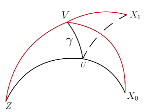
Figure 2. Geometry of Lemma 2.30, if there are two distinct points $X_{0}$ and $X_{1}$ instead of just one $X$.

Consider the two triangles $\triangle ZUV$ and $\triangle UV^{\!}X$ in $S_{\bar{\mu}}$. Since $\mathbf{d}_{s}(U,V)<\pi$,

$$\lvert ZU\rvert+\lvert UV\rvert+\lvert ZV\rvert+\lvert UV\rvert+\lvert UX\rvert+\lvert V^{\!}X\rvert =\lvert ZU\rvert+\lvert UX\rvert+\lvert ZV\rvert+\lvert V^{\!}X\rvert+2\lvert UV\rvert$$

$$=\lvert ZX\rvert+\lvert ZX\rvert+2\lvert UV\rvert$$

$$<4\pi.$$

So the perimeter of either $\triangle ZUV$ or $\triangle UV^{\!}X$ (or both) is less than $2\pi$. Supposing that the perimeter of $\triangle ZUV$ is less than $2\pi$, proceed to construct a congruent triangle $\triangle Z^{\prime}U^{\prime}V^{\prime}$ on the unit sphere. The other case—when the perimeter of $\triangle UV^{\!}X$ is less than $2\pi$—works similarly.

Construct a congruent model on the Euclidean unit sphere of dimension $2$ with $Z^{\prime}$ at the north pole and $X^{\prime}$ at the south pole, where notationally a prime denotes passage to the congruent Euclidean spherical model. Let $\sigma_{0}^{\prime}$ and $\tau_{0}^{\prime}$ be any two half great circles from pole to pole. Pick a point $V^{\prime}$ on $\sigma^{\prime}_{0}$ satisfying $|V^{\prime}Z^{\prime}|=|VZ|$ and a point $U^{\prime}$ on $\tau_{0}^{\prime}$ satisfying $|U^{\prime}Z^{\prime}|=|UZ|$. Now slide $\sigma_{0}^{\prime}$ closer to or further from $\tau_{0}^{\prime}$ so that the shortest path $\gamma^{\prime}$ from $U^{\prime}$ to $V^{\prime}$ has length $|U^{\prime}V^{\prime}|=|UV|$, which is possible because $|UV|<\pi$. Then $\triangle U^{\prime}V^{\prime}Z^{\prime}$ and $\triangle X^{\prime}U^{\prime}V^{\prime}$ are two triangles in a space of constant curvature $1$ congruent to $\triangle UVZ$ and $\triangle XUV$, respectively. For any point $W\in\gamma$ pick a corresponding point $W^{\prime}\in\gamma^{\prime}$. As $(S_{\bar{\mu}}\mathcal{M},d_{s})$ is a $\operatorname{CAT}(1)$ space (that much is true for any locally compact $\operatorname{CAT}(\kappa)$ space by [MMT23a, Corollary 1.25]),

$$|Z^{\prime}W^{\prime}|\geq|ZW|\text{, and }|X^{\prime}W^{\prime}|\geq|XW|,$$

which implies

$$\pi=|Z^{\prime}W^{\prime}|+|X^{\prime}W^{\prime}|\geq|ZW|+|XW|\geq|ZX|=\pi.$$

Thus equalities must occur throughout, and hence

(2.16) $$|ZW|+|WX|=|ZX|=\pi.$$

Therefore (2.15) is proved, so $W\in\Delta$ as desired. ∎

Proof of Proposition 2.29.

Suppose, contrary to the conclusion of the Proposition, that distinct unit vectors $X_{0},X_{1}\in C_{\mu}$ have angles with $Z$ both $\geq\pi$. The goal is to conclude that one of $X_{0}$ and $X_{1}$ does not lie in the convex cone $\operatorname{hull}\mu$ generated by the support of ${\widehat{\mu}}=(\log_{\bar{\mu}})_{\sharp}\mu$. In fact the argument shows that neither $X_{0}$ nor $X_{1}$ lies in $\operatorname{hull}\mu$.

Lemma 2.16 implies that $\angle(Z,X_{0})=\pi=\angle(Z,X_{1})$ and that for $\mu$-almost all $x\in\mathcal{M}$,

$$\angle(\log_{\bar{\mu}}x,Z)+\angle(\log_{\bar{\mu}}x,X_{0})=\pi=\angle(\log_{\bar{\mu}}x,Z)+\angle(\log_{\bar{\mu}}x,X_{1}).$$

Lemma 2.30, applied to $X_{i}$ for $i\in\{0,1\}$, yields convex sets $\mathcal{K}_{i}\subseteq T_{\bar{\mu}}\mathcal{M}$ with

$$\mathcal{K}_{i}=\bigl{\{}Y\in T_{\bar{\mu}}\mathcal{M}\mid\angle(Y,Z)+\angle(Y,X_{i})=\pi\bigr{\}}.$$

Thus the convex cone $\operatorname{hull}\mu$ is contained in the convex set

$$\mathcal{K}=\mathcal{K}_{0}\cap\mathcal{K}_{1}.$$

Now simply note that $X_{0}$ and $X_{1}$ are not in $\mathcal{K}$ as $X_{0}\not\in\mathcal{K}_{1}$ and $X_{1}\not\in\mathcal{K}_{0}$. Thus neither $X_{0}$ nor $X_{1}$ lies in $\operatorname{hull}\mu$. ∎

Corollary 2.31.

Fix a localized measure $\mu$ on a $\operatorname{CAT}(\kappa)$ metric space. For any escape vector $Z\in E_{\mu}$ the restriction $\mathcal{L}_{Z}|_{C_{\mu}}:C_{\mu}\to\nolinebreak\mathcal{L}_{Z}(C_{\mu})$ of the limit log map along $Z$ to the fluctuating cone is an isometry onto its image.

Proof.

Let $\mathcal{K}=C_{\mu}$ in Theorem 1.16 via Proposition 2.29. ∎

Remark 2.32.

The isometry in Corollary 2.31 is the miracle that empowers tangential collapse (Section 4) to relate CLTs in singular settings [MMT23d] to recognizable linear CLTs. This isometry is the reason to define fluctuating cones $C_{\mu}$ as distinct from escape cones $E_{\mu}$, because Corollary 2.31 fails for $E_{\mu}$, in general: the Fréchet mean of a measure supported on the spine of an open book [HHL⁺13, Theorem 2.9] can be nudged onto any desired page of the open book by adding a mass on that page, so the escape cone is the entire open book, which collapses under limit log along any individual page.

Remark 2.33.

For collapse by iterative dévissage in Section 4, assuming the isometry in Corollary 2.31 would suffice instead of the stronger localized hypothesis on $\mu$. What the localized hypothesis adds is convexity of the Fréchet function (Proposition 2.9). That convexity is used for estimates in subsequent work [MMT23d]; but again, localized might be too strong a hypothesis for optimal generality in that regard, as well.

3. Smoothly stratified metric spaces

Definition 3.1 (Smoothly stratified metric space).

A complete, geodesic, locally compact $\operatorname{CAT}(\kappa)$ space $(\mathcal{M},\mathbf{d})$ is a smoothly stratified metric space if it decomposes

$$\mathcal{M}=\bigsqcup_{j=0}^{d}\mathcal{M}^{j}$$

into disjoint locally closed strata $\mathcal{M}^{j}$ so that for each $j$, the stratum $\mathcal{M}^{j}$ has closure

$$\overline{\mathcal{M}^{j}}=\bigcup_{k\leq j}\mathcal{M}^{k},$$

and the following conditions hold.

1. (Manifold strata). For each stratum $\mathcal{M}^{j}$, the space $(\mathcal{M}^{j},\mathbf{d}|_{\mathcal{M}^{j}})$ is a smooth manifold with geodesic distance $\mathbf{d}|_{\mathcal{M}^{j}}$ that is the restriction of $\mathbf{d}$ to $\mathcal{M}^{j}$.

2. (Local exponential maps). For any point $p\in\mathcal{M}$, there exists $\varepsilon>0$ such that the restriction of the logarithm map $\log_{p}$ to an open ball $B(p,\varepsilon)\subseteq\mathcal{M}$ is a homeomorphism, so the exponential map $\exp_{p}=\log_{p}^{-1}$ is locally well defined and a homeomorphism.

Remark 3.2.

Local compactness implies that the space of directions is compact because it is homeomorphic to a compact sphere of small radius around the apex by Definition 3.1.2.

Remark 3.3.

For our purposes, the exponential map is only required to behave well near the Fréchet mean. Thus the main results of this paper continue to hold if the sample space has bad points—where the singularities get worse—outside a ball of positive radius around the Fréchet mean ${\bar{\mu}}$.

Remark 3.4.

Axioms for stratified spaces often include hypotheses explicitly or implicitly designed to force local triviality of tangent data within each stratum. That role is played here by local exponential maps in Definition 3.1.2. Local triviality is not needed for the developments here or in the sequels, [MMT23c] and [MMT23d], so a proof of it (based on radial transport [MMT23a, Definition 2.7 and Proposition 2.8]) is omitted.

Remark 3.5.

Our definition of smoothly stratified metric space does not require a Riemannian structure on each stratum. That is because angles—and thus inner products—on the tangent bundle are not required to vary smoothly. Indeed, angles on a smoothly stratified metric space can be discontinuous (see [MMT23a, Remark 1.22]). Potential alternatives to the existence of local exponential maps in Definition 3.1.2 include Pflaum’s Riemannian stratified spaces [Pfl01] or iterated edge metrics of Albin, Leichtnam, Mazzeo, and Piazza [ALMP12], but issues arise with these.

1. In Pflaum’s definition, a vector flow at a singular point $p$ cannot leave the singular stratum containing $p$, so control is relinquished over the behavior of angles and geodesics near singular points.

2. Similarly, [BKMR18] note that local behavior of geodesics near singular points are not well understood when $\mathcal{M}$ is equipped with an iterated edge metric.

3. It might be possible to replace Definition 3.1.1 with a requirement that the metric $\mathbf{d}$ induces a Riemannian metric on each stratum $\mathcal{M}^{j}$. However, similar to Pflaum’s Riemannian stratified spaces [Pfl01], this does not guarantee control of geodesics near singular points.

Weakenings of the Riemannian framework on manifolds, such as connection spaces [PL20], which still retain enough structure to take derivatives and exponentials could be useful in stratified settings, but for the present purpose remain too strong, as limit log maps (Definition 1.10) only require parallel transport in radial directions (see [MMT23a, Section 2] for details about radial transport).

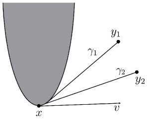
Figure 3. $\exp_{x}$ is not well defined

Remark 3.6.

Definition 3.1.2 should be compared with existence of maximal tubular neighborhoods on stratified spaces via the exponential map on stratified spaces studied by Pflaum [Pfl01]. Example 3.7 is a scenario when the maximal tubular neighborhood of the parabola stratum $\mathcal{M}^{0}$ exists while Definition 3.1.2 is not satisfied.

Example 3.7.

Let $\mathcal{M}=\{(x,y)\in\mathbb{R}^{2}\mid y\leq x^{2}\}$ (Figure 3) be the space with strata

• $\mathcal{M}^{0}=\{(x,y)\in\mathbb{R}^{2}\mid y=x^{2}\}$

• $\mathcal{M}^{1}=\mathcal{M}\setminus M_{0}$

whose metric on $\mathcal{M}^{1}$ is the induced flat metric from $\mathbb{R}^{2}$ and whose metric on $\mathcal{M}^{2}$ is the curve length metric on the parabola $y=x^{2}$. For a piecewise smooth curve $\gamma$ in $\mathcal{M}$, the length of $\gamma$ is the sum of the length of the intersection with $\mathcal{M}^{0}$ and $\mathcal{M}^{1}$,

$$|\gamma|=|\gamma\cup\mathcal{M}^{0}|+|\gamma\cap\mathcal{M}^{1}|.$$

The metric on $\mathcal{M}$ is defined as

$$\mathbf{d}(x,y)=\inf_{\begin{subarray}{c}\gamma:[0,1]\to\mathcal{M}\ \\ \gamma[0]=x,\ \gamma[1]=y\end{subarray}}|\gamma|.$$

Then $(\mathcal{M},\mathbf{d})$ is a length space and also a Riemannian stratified space in the sense of Pflaum [Pfl01, Definition 2.4.1]. But it is not a smoothly stratified metric space by Definition 3.1 since the exponential map at $x$ is not locally defined.

It bears mentioning that this example reflects a geometric problem and not a topological one: the fact that $\mathcal{M}$ has nonempty boundary is not the issue. Indeed, the discussion would still work after taking the union of $\mathcal{M}$ with a half-infinite cylinder with the parabola as its base, the union being homeomorphic to the plane $\mathbb{R}^{2}$.

Remark 3.8.

The tangent cone at a singular point $p$ of a stratified space is often thought of as a product of the vectors tangent to the stratum containing $p$ and a normal cone of vectors pointing out of the stratum. The normal cone is a cone over its unit vectors, which form the link of the singular point. The topological type of the link reflects the nature of the singularity type (see [GM88, p. 7], for example), with smooth points having links that are spheres, mildly singular points having smooth links, and deeper singularities having links that are one step less singular. In this metric setting, however, even a point whose link is a sphere can be singular; that occurs, for example, in the kale [HMMN15], which is homeomorphic to a Euclidean plane but not isometric to it, having an isolated point of angle sum $>2\pi$. Since part of our theory collapses by inductively reducing the “depth” of a singularity at $p$ via limits of tangent cones upon approach to $p$ (Section 4), a proxy is needed to bound the “depth” of the singularity to guarantee that this procedure terminates. For that purpose, the codimension of the stratum containing $p$ suffices, as follows, since the codimension increases by at least $1$ with each iterated cone over a link. Definition 3.9 is used only in Proposition 4.18.

Definition 3.9.

A point $p$ in a smoothly stratified metric space $\mathcal{M}$ has codimension

$$\operatorname{codim}p=M-m,$$

where $m$ is the dimension of the (unique smallest) stratum containing $p$ and $M$ is the maximal dimension of any stratum whose closure contains $p$.

Remark 3.10.

Points of lower codimension should be thought of as less singular than points of higher codimension. Although the set of singular points is larger when the codimension is smaller, that set is just a stratum’s worth of copies of the same singularity. The type of the singularity is recorded more faithfully by the normal cone, whose dimension decreases along with the codimension.

This subsection concludes with crucial components of tangential collapse in Section 4, extensions of the geometry in Section 1 available in the smoothly stratified setting. The first reduces from the setting of smoothly stratified metric spaces, where curvature is bounded above by $\kappa$, to nonpositively curved tangent cones, where curvature is bounded above by $0$. It is applied in the proof of Proposition 4.18.

Proposition 3.11.

The conical metric on $T_{p}\mathcal{M}$ makes the tangent cone of any point $p$ in a smoothly stratified metric space $\mathcal{M}$ a smoothly stratified nonpositively curved space.

Proof.

The space is nonpositively curved by Lemma 1.13. The stratification decomposes into disjoint strata appropriately for Definition 3.1 because $\mathcal{M}$ itself does and local exponentiation is a homeomorphism in Definition 3.1.2. The metric on $T_{p}\mathcal{M}$ is induced (via angles in Definition 1.1 and Lemma 1.2) by the metric on $\mathcal{M}$ itself, which restricts appropriately to its strata by Definition 3.1.2. Therefore the metric on $T_{p}\mathcal{M}$ restricts appropriately for Definition 3.1.1 because of how the conical metric on $T_{p}\mathcal{M}$ is constructed in Definitions 1.3 and 1.6. ∎

The next result is applied in the last step of tangential collapse (Proposition 4.20).

Lemma 3.12.

In the situation of Proposition 3.11, geodesic projection of $T_{p}\mathcal{M}$ onto the tangent vector space at $p$ of the stratum $R$ containing $p$, namely

$$\mathbf{P}:T_{p}\mathcal{M} \to T_{p}R$$

$$W \mapsto\operatorname*{argmin}_{Z\in T_{p}R}\mathbf{d}_{p}(Z,W)$$

is a contraction, in the sense that it weakly decreases angles: for $Z\!\in T_{p}R$ and $V\!\in\nolinebreak T_{p}\mathcal{M}$,

$$\langle\mathbf{P}(V),Z\rangle_{p}\geq\langle V,Z\rangle_{p}.$$

Proof.

For readability, set $W=\mathbf{P}(V)$, write $\mathcal{O}$ for the apex of the tangent cone $T_{p}R\subseteq T_{p}\mathcal{M}$, and omit the subscripts on pairings. Assume $W\neq\mathcal{O}$ and $V\notin T_{\mathcal{O}}R$ is not already tangent to $R$, since otherwise $W=V$ and equality on the pairings is trivial. Note that $\angle(V,W)<\pi/2$ because otherwise $\mathbf{d}_{\mathcal{O}}(V,\mathcal{O})\leq\mathbf{d}_{\mathcal{O}}(V,W)$, which violates the definition of $\mathbf{P}(V)$.

In what follows, for $U,V\in T_{\mathcal{O}}\mathcal{M}$ write $UV$ to mean the shortest path from $U$ to $V$ and $|UV|$ to mean the length $\mathbf{d}_{\mathcal{O}}(U,V)$ of this path.

Figure 4.

The triangle $\triangle VWZ$ in the $\operatorname{CAT}(0)$ space $T_{\mathcal{O}}\mathcal{M}$ has $\angle(WV,WZ)\geq\pi/2$ by [BH13, Proposition 2.4] because $W$ is the projection of $V$, so

(3.1) $$|VZ|^{2}\geq|VW|^{2}+|WZ|^{2}.$$

Invoke Lemma 1.7 to see that the triangle $\triangle V\mathcal{O}Z$ is flat. Rescaling if necessary, assume that $V$ and $Z$ are unit vectors. The law of cosines applied to them yields

(3.2) $$|VZ|^{2}=2-2\langle V,Z\rangle.$$

Combing (3.1) and (3.2) produces

(3.3) $$2\langle V,Z\rangle\leq 2-|VW|^{2}-|WZ|^{2}.$$

Now observe that the triangle $\triangle V\mathcal{O}W$ is also flat (by applying Lemma 1.7 again) and $\angle(WV,W\mathcal{O})=\pi/2$, so

(3.4) $$1=|\mathcal{O}V|^{2}=|\mathcal{O}W|^{2}+|VW|^{2}.$$

From (3.3) and (3.4) we obtain

(3.5) $$2\langle V,Z\rangle\leq 1+|\mathcal{O}W|^{2}-|WZ|^{2}=|\mathcal{O}Z|^{2}+|\mathcal{O}W|^{2}-|WZ|^{2}=2\langle W,Z\rangle$$

where the last equality comes from the law of cosines in the triangle $\triangle\mathcal{O}WZ$, which is again flat by Lemma 1.7. Thus $\langle V,Z\rangle\leq\langle W,Z\rangle$, as desired. ∎

The final result in this section is used in the proof of Proposition 4.20 on the way to existence of tangential collapse in Theorem 4.21. It says that after taking limit log, the escape cone always includes the stratum containing the mean.

Proposition 3.13.

Under Hypotheses 2.22, assume in addition that $\mathcal{M}$ is smoothly stratified. Suppose $\mathcal{L}_{Z}(Z)$ lies in a stratum $\smash{\makebox[0.0pt][l]{$T$}\raisebox{6.02773pt}{\scalebox{1.1}[0.5]{${}^{\rightarrow\!\!}$}}}_{Z}R\subseteq\smash{\makebox[0.0pt][l]{$T$}\raisebox{6.02773pt}{\scalebox{1.1}[0.5]{${}^{\rightarrow\!\!}$}}}_{Z}\mathcal{M}$, where $R$ is the stratum of $\mathcal{M}$ toward which $Z$ points. Then the escape cone $E_{\mu_{Z}}$ of $\mu_{Z}$ contains the vector space $\smash{\makebox[0.0pt][l]{$T$}\raisebox{6.02773pt}{\scalebox{1.1}[0.5]{${}^{\rightarrow\!\!}$}}}_{Z}R$.

Proof.

The goal is to show that, for all $V_{Z}\in\smash{\makebox[0.0pt][l]{$T$}\raisebox{6.02773pt}{\scalebox{1.1}[0.5]{${}^{\rightarrow\!\!}$}}}_{Z}R$,

$$\nabla_{\!{\bar{\mu}}_{Z}}F_{\mu_{Z}}(V_{Z})=0.$$

Recall from (2.8) that

$$\nabla_{{\bar{\mu}}}F_{\mu_{Z}}(\mathcal{L}_{Z}Z)=\nabla_{{\bar{\mu}}}F_{\widehat{\mu}}(Z)=0.$$

Applying Lemma 1.15 and Corollary 2.7 yields

$$-\nabla_{\!{\bar{\mu}}_{Z}}F_{\mu_{Z}}(\mathcal{L}_{Z}Z) =\int_{\smash{\makebox[0.0pt][l]{$T$}\raisebox{4.2194pt}{\scalebox{1.1}[0.5]{${}^{\rightarrow\!\!}$}}}_{Z}\mathcal{M}}\langle\mathcal{L}_{Z}Z,W_{z}\rangle\mu_{Z}(dW_{z})$$

$$=-\int_{\smash{\makebox[0.0pt][l]{$T$}\raisebox{4.2194pt}{\scalebox{1.1}[0.5]{${}^{\rightarrow\!\!}$}}}_{Z}\mathcal{M}}\langle-\mathcal{L}_{Z}Z,W_{z}\rangle\mu_{Z}(dW_{z})$$

$$=\nabla_{{\bar{\mu}}}F_{\mu_{Z}}(-\mathcal{L}_{Z}Z).$$

Consequently,

$$\nabla_{\!{\bar{\mu}}_{Z}}F_{\mu_{Z}}(-\mathcal{L}_{Z}Z)=\nabla_{\!{\bar{\mu}}_{Z}}F_{\mu_{Z}}(\mathcal{L}_{Z}Z)=0.$$

Combine this with the fact that ${\bar{\mu}}_{Z}$ minimizes the convex function $F_{\mu_{Z}}$, so the directional derivative $\nabla_{\!{\bar{\mu}}_{Z}}F_{\mu_{Z}}$ is convex and nonnegative on the Euclidean space $\smash{\makebox[0.0pt][l]{$T$}\raisebox{6.02773pt}{\scalebox{1.1}[0.5]{${}^{\rightarrow\!\!}$}}}_{Z}R$, to get

$$\nabla_{\!{\bar{\mu}}_{Z}}F_{\mu_{Z}}(V_{Z})=0\text{ for all }V_{Z}\in\smash{\makebox[0.0pt][l]{$T$}\raisebox{6.02773pt}{\scalebox{1.1}[0.5]{${}^{\rightarrow\!\!}$}}}_{Z}R.\qed$$

4. Tangential collapse

The goal is to embed the fluctuating cone $C_{\mu}$ into a Euclidean space by collapsing the local singularity at the Fréchet mean (Theorem 4.21). This is done by a series of dévissage steps, each taking a limit logarithm along a resolving direction. Each dévissage (Definition 4.5) pushes forward the measure $\mu$ under the limit log along a resolving direction. The result is a measure on a stratified space whose singularity has lower codimension (Definition 3.9) and is thus less singular.

Results throughout this section specify certain hypotheses, so it is important to recall these, especially localization (Definition 2.1) for measures on smoothly stratified metric spaces (Definition 3.1). Note also that the collapse by iterative dévissage heavily involves limit log maps (Definition 1.10) along resolving directions (Definition 4.2).

4.1. Dévissage

Proposition 4.1.

Fix a localized measure $\mu$ on a smoothly stratified metric space $\mathcal{M}$. For any unit vector $Z$ in the escape cone $E_{\mu}$ (Definition 2.12) let $\mu_{Z}=(\mathcal{L}_{Z})_{\sharp}{\widehat{\mu}}$ be the pushforward of ${\widehat{\mu}}=(\log_{\bar{\mu}})_{\sharp}\mu$ under limit log map along $Z$. Then

1. ${\bar{\mu}}_{Z}=\mathcal{L}_{Z}{\bar{\mu}}$ is the Fréchet mean of $\mu_{Z}$;

2. $\mathcal{L}_{Z}$ maps the fluctuating cone $C_{\mu}$ isometrically to its image, so for all $V,W\in C_{\mu}$,

   $$\angle\bigl{(}\mathcal{L}_{Z}(V),\mathcal{L}_{Z}(W)\bigr{)}=\angle(V,W);$$

3. the fluctuating cone $C_{\mu_{Z}}$ of $\mu_{Z}$ satisfies $\mathcal{L}_{Z}(C_{\mu})\subseteq C_{\mu_{Z}}$;

4. the measure $\mu_{Z}$ is localized.

Proof.

The first claim comes from Proposition 2.26 (see also Lemma 2.11), and the second one comes from Corollary 2.31, both of which use the localized hypothesis. The third is Corollary 2.28. For the fourth, $\mu_{Z}$ is automatically localized by Example 2.2 because by Lemma 1.13 the limit tangent cone $\smash{\makebox[0.0pt][l]{$T$}\raisebox{6.02773pt}{\scalebox{1.1}[0.5]{${}^{\rightarrow\!\!}$}}}_{Z}\mathcal{M}$ is $\operatorname{CAT}(0)$. ∎

Definition 4.2.

A resolving direction for a measure $\mu$ on a smoothly stratified $\operatorname{CAT}(\kappa)$ metric space is a unit vector in the fluctuating cone $C_{\mu}$ pointing to a stratum of highest dimension among strata having nonempty intersection with the exponential image

$$\{\exp_{\bar{\mu}}V\mid V\in C_{\mu}\text{ can be exponentiated}\}$$

of the fluctuating cone as per Definition 3.1.2.

Remark 4.3.

Proposition 4.1 implies that applying the limit log map along a resolving direction results in a stratified space with the Fréchet mean ${\bar{\mu}}$ and the fluctuating cone $C_{\mu}$ preserved. It turns out that ${\bar{\mu}}$ and $C_{\mu}$ is all of the information needed to reproduce the limiting distribution for the CLT in a less singular stratified space; see the Perturbative CLT in [MMT23d, Section 6.2]. And it is the essence of dévissage in Definitions 4.5 and 4.8: collapse by iterating the limit log map in Proposition 4.1. Conditions for this iteration occupy Definition 4.4.

Definition 4.4.

A ravel is a triple $\{\mathcal{M},\nu,V\}$ where $\mathcal{M}$ is a smoothly stratified metric space, $\nu$ is a probability measure on $\mathcal{M}$, and $V$ is a resolving direction of $\nu$.

Definition 4.5.

Given a ravel $\{\mathcal{M},\nu,V\}$, a dévissage step takes a limit log along the direction $V$ to transfer the ravel $\{\mathcal{M},\nu,V\}$ to a new one $\{\mathcal{M}^{\prime},\nu\hskip 1.07639pt^{\prime},V^{\prime}\}$, where

1. $\mathcal{M}^{\prime}=\mathcal{L}_{V}(\mathcal{M})$,

2. $\nu\hskip 1.07639pt^{\prime}=(\mathcal{L}_{V})_{\sharp}\nu$, and

3. $V^{\prime}$ is a resolving direction of $\nu\hskip 1.07639pt^{\prime}$.

Definition 4.6.

Fix a ravel $\{\mathcal{M},\nu,V\}$ whose Fréchet mean ${\bar{\nu}}$ lies in a stratum $R$. The ravel $\{\mathcal{M},\nu,V\}$ is resolved if $C_{\nu}\subseteq T_{\bar{\nu}}R$. Otherwise, $\{\mathcal{M},\nu,V\}$ is unresolved.

Remark 4.7.

When a ravel $\{\mathcal{M},\nu,V\}$ is unresolved, the local geometry can be improved, in the sense that the singularity codimension can be reduced by taking the limit log map along a resolving direction, as in Proposition 4.1. When $\{\mathcal{M},\nu,V\}$ is resolved, however, the limit log map is constrained to take place within the same stratum as the Fréchet mean ${\bar{\nu}}$, so the limit tangent cone at ${\bar{\nu}}$ has the same singularity as the tangent cone at ${\bar{\nu}}$ itself. The process of dévissage here, made precise in Definition 4.8, is a sequence of dévissage steps (thought of as “unravelings”) applied to unresolved ravels until a resolved ravel is achieved.

The starting ravel of interest is the tangent cone $\{T_{\bar{\mu}}\mathcal{M},{\widehat{\mu}},Z\}$, where ${\widehat{\mu}}=(\log_{\bar{\mu}})_{\sharp}\mu$ is pushed forward from $\mathcal{M}$ to the tangent cone under the log map, as usual.

Definition 4.8.

Fix a measure $\mu$ on a smoothly stratified metric space $\mathcal{M}$. The process of dévissage is a sequence of dévissage steps, beginning with an initial ravel $\{\mathcal{M}_{0},\nu_{0},Z_{0}\}=\{T_{\bar{\mu}}\mathcal{M},{\widehat{\mu}},Z\}$ for any resolving direction $Z$ of $\mu$ and whose step $i$ applies a dévissage step to the ravel $\{\mathcal{M}_{i},\nu_{i},Z_{i}\}$ to produce the ravel $\{\mathcal{M}_{i+1},\nu_{i+1},Z_{i+1}\}$, where

1. $\mathcal{M}_{i+1}=\smash{\makebox[0.0pt][l]{$T$}\raisebox{6.02773pt}{\scalebox{1.1}[0.5]{${}^{\rightarrow\!\!}$}}}_{Z_{i}}(\mathcal{M}_{i})$,

2. $\nu_{i+1}=(\mathcal{L}_{Z_{i}})_{\sharp}\nu_{i}$, and

3. $Z_{i+1}$ is a resolving direction of $\nu_{i+1}$.

The dévissage terminates at step $k$ when the ravel $\{\mathcal{M}_{k+1},\nu_{k+1},Z_{k+1}\}$ is resolved (Definition 4.6). To simplify notation in discussions of dévissage, let

• $\mathcal{L}_{i}=\mathcal{L}_{Z_{i}}$ be the limit logarithm map along direction $Z_{i}$,

• $C_{i}=C_{\nu_{i}}$ be the fluctuating cone of $\nu_{i}$, and

• $\mathbf{d}_{i}=\mathbf{d}_{{\bar{\nu}}_{i}}$ be the conical distance function on $\mathcal{M}_{i}$ (Definition 1.6).

If termination occurs at step $k$, then write

• $\mathcal{M}_{\infty}=\mathcal{M}_{k+1}$ for the terminal smoothly stratified metric space,

• $\nu_{\infty}=\nu_{k+1}$ for the terminal measure on $\mathcal{M}_{\infty}$,

• $\mathbf{d}_{\infty}=\mathbf{d}_{{\bar{\nu}}_{\infty}}$ for the terminal distance function on $\mathcal{M}_{\infty}$,

• $R_{\infty}$ for the terminal stratum of $\mathcal{M}_{\infty}$ that contains ${\bar{\nu}}_{\infty}$,

• $T_{\infty}=T_{{\bar{\nu}}_{\infty}}R_{\infty}\cong\mathbb{R}^{\dim R_{\infty}}$ for the terminal tangent vector space,

• $C_{\infty}=C_{\nu_{\infty}}\subseteq T_{\infty}$ for the terminal fluctuating cone, and

• $Z_{\infty}=Z_{k}\in T_{\infty}$ for the terminal resolving direction.

Remark 4.9.

Dévissage terminates when resolving directions fail to point out of the current Fréchet mean stratum, so further limit logarithms along resolving directions do not reduce the singularity codimension. That happens, for example, when the last dévissage moves to a top stratum, i.e., with codimension $0$. But it is possible for dévissage to stick to a stratum of positive codimension. Such is the case when $\mathcal{M}$ is an open book [HHL⁺13], where the Fréchet mean is confined to the spine.

Lemma 4.10.

In any dévissage from Definition 4.8, $\mathcal{L}_{i}({\bar{\nu}}_{i})={\bar{\nu}}_{i+1}$ and the singularity at ${\bar{\nu}}_{i+1}$ has strictly lower codimension than at ${\bar{\nu}}_{i}$.

Proof.

The Fréchet mean equality is thanks to Proposition 4.1. What remains is to carry out the dimension calculation showing that dévissage (Definition 4.5) applied to an unresolved ravel $\{\mathcal{M},\nu,V\}$ reduces the codimension of the singularity by at least $1$ upon passage to $\{\mathcal{M}^{\prime},\nu\hskip 1.07639pt^{\prime},V^{\prime}\}$. Let $R$ be the stratum of $\mathcal{M}$ containing ${\bar{\nu}}$. By Definition 4.6 of unresolved, the exponential of $tV$ for positive $t\ll 1$ lies in a stratum $R^{\prime}$ of $\mathcal{M}$ that does not equal $R$ but whose closure meets $R$, as can be seen by letting $t\to\nolinebreak 0$. The stratum of $\mathcal{M}^{\prime}$ containing ${\bar{\nu}}\hskip 1.07639pt^{\prime}$ contains $T_{{\bar{\nu}}\hskip 0.75346pt^{\prime}}R^{\prime}$ and hence has strictly larger dimension than $R$ does. Similarly, any stratum whose closure meets $R^{\prime}$ also contains $R$ in its closure; taking tangent cones implies that the maximal dimension of a stratum containing ${\bar{\nu}}\hskip 1.07639pt^{\prime}$ is at most the maximal dimension of a stratum whose closure contains $R$. ∎

Remark 4.11.

The notations $\mathcal{M}_{\infty}$ and ${\bar{\nu}}_{\infty}$ and so on for the terminal objects are justified because any attempt at dévissage beyond termination would have no effect: the relevant limit log map would be the identity, or at least a canonical isometry.

The purpose of dévissage is to map the singular situation surrounding the fluctuating cone of $\mu$ in $\mathcal{M}$ to a smooth version. The heavy lifting is carried by composing the dévissage steps.

Definition 4.12.

The composite dévissage is

$$\mathcal{L}_{\circ}=\mathcal{L}_{k}\circ\dots\circ\mathcal{L}_{0}:T_{\bar{\mu}}\mathcal{M}\to\smash{\makebox[0.0pt][l]{$T$}\raisebox{6.02773pt}{\scalebox{1.1}[0.5]{${}^{\rightarrow\!\!}$}}}_{Z_{k}}\mathcal{M}_{k}=\mathcal{M}_{\infty}.$$

Alas, although the target of $\mathcal{L}_{\circ}$ is smooth when the last dévissage step moves to a top stratum, it need not be smooth in general. Therefore $\mathcal{L}_{\circ}$ in general only produces a partial tangential collapse, in the following sense.

Definition 4.13 (Tangential collapse).

Fix a measure $\mu$ on a smoothly stratified metric space $\mathcal{M}$, and let $T$ be a conical (Definition 1.8) smoothly stratified metric space. A partial tangential collapse of $\mu$ with target $T$ is a map $\mathcal{L}:T_{\bar{\mu}}\mathcal{M}\to T$ such that

1. $\mathcal{L}\bigl{(}\log_{\bar{\mu}}({\bar{\mu}})\bigr{)}=0$ is the Fréchet mean of the pushforward $\mathcal{L}_{\sharp}{\widehat{\mu}}$, where ${\widehat{\mu}}=(\log_{\bar{\mu}})_{\sharp}\mu$;

2. $\mathcal{L}$ is injective on the closure ${\hskip 0.86108pt\overline{C}\hskip 0.86108pt}_{\mu}$ of the fluctuating cone $C_{\mu}\subseteq T_{\bar{\mu}}\mathcal{M}$;

3. for any fluctuating vector $U\in C_{\mu}$ and any tangent vector $V\in T_{\bar{\mu}}\mathcal{M}$,

   $$\langle U,V\rangle_{\bar{\mu}}=\bigl{\langle}\mathcal{L}(U),\mathcal{L}(V)\bigr{\rangle}_{\mathcal{L}({\bar{\mu}})}.$$

4. $\mathcal{L}$ is homogeneous: $\mathcal{L}(tV)=t\mathcal{L}(V)$ for all real $t\geq 0$ and $V\in T_{\bar{\mu}}\mathcal{M}$; and

5. $\mathcal{L}$ is continuous.

A (full) tangential collapse of $\mu$ is a partial collapse $\mathcal{L}:T_{\bar{\mu}}\mathcal{M}\to\nolinebreak\mathbb{R}^{m}$ whose target is a vector space.

Remark 4.14.

Angle preservation for $V\in C_{\mu}$ in Definition 4.13.3 and continuity means the restriction of $\mathcal{L}$ from ${\hskip 0.86108pt\overline{C}\hskip 0.86108pt}_{\mu}$ to its image makes the map ${\hskip 0.86108pt\overline{C}\hskip 0.86108pt}_{\mu}\to\mathcal{L}(C_{\mu})$ an isometry.

To reach a full tangential collapse, composite dévissage $\mathcal{L}_{\circ}$ must be followed by terminal projection to squash the singular cone $\smash{\makebox[0.0pt][l]{$T$}\raisebox{6.02773pt}{\scalebox{1.1}[0.5]{${}^{\rightarrow\!\!}$}}}_{Z_{k}}\mathcal{M}_{k}$ onto the (automatially Euclidean) tangent space to the stratum containing the terminal Fréchet mean.

Definition 4.15.

Given a dévissage process, the terminal projection is the geodesic projection of $T_{{\bar{\nu}}_{\infty}}\mathcal{M}_{\infty}$ onto the terminal tangent vector space $T_{\infty}=T_{{\bar{\nu}}_{\infty}}R_{\infty}$, namely

(4.1) $$\begin{split}\mathbf{P}_{\infty}:T_{{\bar{\nu}}_{\infty}}\mathcal{M}_{\infty}&\to T_{\infty}\\ W&\mapsto\operatorname*{argmin}_{Z\in T_{\infty}}\mathbf{d}_{\infty}(Z,W).\end{split}$$

Remark 4.16.

Terminal projection $\mathbf{P}_{\infty}$ restricts to the identity on $T_{\infty}$. Therefore $(\mathbf{P}_{\infty}\circ\mathcal{L}_{\circ})|_{C_{\mu}}$ is an isometry and $\mathbf{P}_{\infty}\circ\mathcal{L}_{\circ}({\bar{\mu}})$ is the Fréchet mean of $(\mathbf{P}_{\infty}\circ\mathcal{L}_{\circ})_{\sharp}{\widehat{\mu}}$. When the last dévissage step moves to a top stratum, $\mathbf{P}_{\infty}$ is the identity map on $T_{\infty}$ because $R_{\infty}$ is then a top stratum, so there are no tangent vectors outside of $T_{{\bar{\nu}}_{\infty}}R_{\infty}$; thus $\mathbf{P}_{\infty}\circ\mathcal{L}_{\circ}=\mathcal{L}_{\circ}$ in that case. See also Corollary 4.19, which implies that the resolution constructed here has slightly stronger properties in that case.

Lemma 4.17.

The terminal projection $\mathbf{P}_{\infty}$ is continuous.

Proof.

Convex projection in a $\operatorname{CAT}(0)$ space contracts [BH13, Proposition II.2.4]. ∎

4.2. Constructing tangential collapse

Throughout this subsection, fix notation as in Definitions 4.8 and 4.15.

Proposition 4.18.

Fix a localized measure $\mu$ on a smoothly stratified metric space $\mathcal{M}$ and a dévissage that terminates at step $k$. For $i=0,\dots,k$,

1. $\nu_{i}$ is localized on the smoothly stratified $\operatorname{CAT}(0)$ space $\mathcal{M}_{i}$;

2. $\mathcal{L}_{i}({\bar{\nu}}_{i})={\bar{\nu}}_{i+1}$ and the singularity at ${\bar{\nu}}_{i+1}$ has strictly lower codimension than at ${\bar{\nu}}_{i}$;

3. $\mathcal{L}_{i}$ isometrically maps $C_{i}$ to $\mathcal{L}_{i}(C_{i})$;

4. the terminal tangent space $T_{\infty}$ is a real vector space;

5. $\mathcal{L}_{i}$ is homogeneous;

6. $\mathcal{L}_{i}$ is continuous; and

7. for all $U\in C_{\mu}$ and all $V\in T_{\bar{\mu}}\mathcal{M}$,

   $$\bigl{\langle}\mathcal{L}_{i}(U),\mathcal{L}_{i}(V)\bigr{\rangle}=\langle U,V\rangle.$$

Proof.

Claim 1 is by Propositions 3.11 and 4.1. Claim 2 is Lemma 4.10. Claim 3 follows from Claim 7. Claim 4 is by Definition 4.8. Claim 5 is by Definition 1.10. Claim 6 is by Claim 5 and Definition 1.6 of conical metric, using contraction in Proposition 1.14.

For Claim 7, let $V$ be any element in $T_{\bar{\mu}}\mathcal{M}$. Given the resolving direction $Z_{0}$ of $\mu$, Proposition 2.26 says that ${\bar{\mu}}_{Z_{0}}=\mathcal{L}_{Z_{0}}({\bar{\mu}})$ is the Fréchet mean of $\nu_{1}=(\mathcal{L}_{Z_{0}})_{\sharp}{\widehat{\mu}}$, so

(4.2) $$\nabla_{\!{\bar{\mu}}_{Z_{0}}}F_{\nu_{0}}(\mathcal{L}_{0}(V))\geq 0\text{ for all }V\in T_{\bar{\mu}}\mathcal{M}$$

because Fréchet means minimize Fréchet functions locally. On the other hand, by contraction under limit log maps in Proposition 1.14,

(4.3) $$\langle U,V\rangle\leq\bigl{\langle}\mathcal{L}_{0}(U),\mathcal{L}_{0}(V)\bigr{\rangle},$$

which can only decrease gradients. Hence for all $U\in C_{\mu}$

(4.4) $$\nabla_{\!{\bar{\mu}}_{Z_{0}}}F_{\nu_{0}}\bigl{(}\mathcal{L}_{0}(U)\bigr{)}\leq\nabla_{\!{\bar{\mu}}}F_{\mu}(U)=0,$$

by Definition 2.18 of fluctuating cone. Combining Eqs. (4.2), (4.3), and (4.4) yields that for $U\in C_{\mu}$ and $V\in T_{\bar{\mu}}\mathcal{M}$,

$$\bigl{\langle}\mathcal{L}_{Z_{0}}(U),\mathcal{L}_{Z_{0}}(V)\bigr{\rangle}=\langle U,V\rangle.$$

Thus, Claim 7 is satisfied for $i=0$ and, by induction, for all $i$. ∎

Corollary 4.19.

Given a localized measure $\mu$ on a smoothly stratified metric space $\mathcal{M}$, the composite dévissage $\mathcal{L}_{\circ}$ in Definition 4.12 is a partial tangential collapse of $\mu$ with target $\mathcal{M}_{\infty}$.

Proof.

By Definition 4.13, this is a direct consequence of Proposition 4.18. ∎

Proposition 4.20.

Fix a localized measure $\mu$ on a smoothly stratified metric space $\mathcal{M}$ and a dévissage (Definition 4.8). Write

• $\mathcal{O}={\bar{\nu}}_{\infty}=\mathbf{P}_{\infty}({\bar{\nu}}_{\infty})$, the origin of the terminal tangent vector space $T_{\infty}$,

• $\mu^{\mathcal{L}}=(\mathbf{P}_{\infty})_{\sharp}\nu_{\infty}$, the resolved measure on $T_{\infty}$, and

• $\mathcal{L}=\mathbf{P}_{\infty}\circ\mathcal{L}_{\circ}$, the terminal collapse

obtained by composing the terminal projection $\mathbf{P}_{\infty}$ in Definition 4.15 with the composite dévissage $\mathcal{L}_{\circ}$ in Definition 4.12. Then

$$\mu^{\mathcal{L}}=\mathcal{L}_{\sharp}{\widehat{\mu}}=(\mathcal{L}\circ\log_{\bar{\mu}})_{\sharp}\mu$$

is the pushforward of ${\widehat{\mu}}=(\log_{\bar{\mu}})_{\sharp}\mu$ under $\mathcal{L}$, and $\mathcal{O}$ is the Fréchet mean of $\mu^{\mathcal{L}}$. In addition, for any $V\in C_{\mu}$ and any $X\in T_{\bar{\mu}}\mathcal{M}$,

(4.5) $$\langle X,V\rangle_{\bar{\mu}}=\bigl{\langle}\mathcal{L}(X),\mathcal{L}(V)\bigr{\rangle}{}_{\mathcal{O}}.$$

Proof.

Since $T_{\mathcal{O}}R_{\infty}=T_{\infty}$ is Euclidean, the Fréchet function $F_{\mu^{\mathcal{L}}}$ of $\mu^{\mathcal{L}}$ on $T_{\mathcal{O}}R_{\infty}$ is differentiable and convex. Furthermore, if ${\bar{\nu}}$ is the Fréchet mean of $\mu^{\mathcal{L}}$, then

$$F_{\mu^{\mathcal{L}}}(x)-F_{\mu^{\mathcal{L}}}({\bar{\nu}})=\frac{1}{2}\mathbf{d}_{\mathcal{O}}(x,{\bar{\nu}})^{2}$$

for any $x\in T_{{\bar{\nu}}}R_{\infty}$. To show that $\mathcal{O}$ minimizes $F_{\mu^{\mathcal{L}}}$, it suffices to show that

(4.6) $$\nabla_{\!\mathcal{O}}F_{\mu^{\mathcal{L}}}(Y)\leq 0$$

for any tangent vector $Y\in T_{\infty}$ to the terminal stratum. Indeed, as $\nabla_{\!\mathcal{O}}F_{\mu^{\mathcal{L}}}(Y)$ is linear in $V$, (4.6) implies that $\nabla_{\!\mathcal{O}}F_{\mu^{\mathcal{L}}}(Y)=0$ for all $Y\in T_{\infty}$. Thus $\mathcal{O}$ is a stationary point of $F_{\mu^{\mathcal{L}}}$. Convexity of $F_{\mu^{\mathcal{L}}}$ implies that $\mathcal{O}$ is the minimizer of $F_{\mu^{\mathcal{L}}}$.

To show (4.6), observe that by Corollary 2.7,

(4.7) $$\nabla_{\!\mathcal{O}}F_{\mu^{\mathcal{L}}}(Y)=-\!\!\int_{T_{\mathcal{O}}R_{\infty}}\langle X,Y\rangle\mu^{\mathcal{L}}(dX) =-\!\!\int_{T_{\mathcal{O}}\mathcal{M}_{\infty}}\bigl{\langle}\mathbf{P}_{\infty}(X),Y\bigr{\rangle}\nu_{\infty}(dX).$$

(4.8) $$\leq-\!\!\int_{T_{\mathcal{O}}\mathcal{M}_{\infty}}\langle X,Y\rangle\nu_{\infty}(dX)\text{ by Lemma~{}\ref{l:decrease-inner-product}}$$

$$=\nabla_{\!\mathcal{O}}F_{\nu_{\infty}}(Y)\leq 0,$$

where $\leq 0$ is because $\mathcal{O}$ minimizes $F_{\nu_{\infty}}$ and $Y\in T_{\infty}\subseteq E_{\mu}$ by Proposition 3.13.

Differentiability of $F_{\mu^{\mathcal{L}}}$ (observed at the proof’s start) and (4.7) yield $\nabla_{\!\mathcal{O}}F_{\mu^{\mathcal{L}}}(V)=0$, which in particular implies equality in (4.8). Together these two equalities yield

$$\bigl{\langle}\mathbf{P}_{\infty}(X),V\bigr{\rangle}=\langle X,V\rangle$$

for $\nu_{\infty}$-almost all $X$, and hence for all $X$ by continuity of $\mathbf{P}_{\infty}$ and of inner products in Lemmas 4.17 and 1.5. Moreover, as $\mathbf{P}_{\infty}(V)=V$, this can be rewritten

$$\bigl{\langle}\mathbf{P}_{\infty}(X),\mathbf{P}_{\infty}(V)\bigr{\rangle}=\langle X,V\rangle$$

for all $X$. From here, (4.5) is a consequence of Corollary 4.19. ∎

Recall the summary of definitions regarding measures and spaces from the paragraph before Section 4.1 and additional definitions concerning dévissage in Definitions 4.8, 4.5, and 4.12, and terminal projection in 4.15.

Theorem 4.21.

Fix a smoothly stratified metric space $\mathcal{M}$ and on it a localized probability measure $\mu$ with Fréchet mean ${\bar{\mu}}$. The terminal collapse $\mathcal{L}=\mathbf{P}_{\infty}\circ\mathcal{L}_{\circ}:T_{\bar{\mu}}\mathcal{M}\to\nolinebreak T_{\infty}$ for any dévissage is a tangential collapse of $\mu$ as in Definition 4.13.

Proof.

After Corollary 4.19 and Proposition 4.20, the only things left to prove are homogeneity and continuity of $\mathcal{L}$, injectivity on the closure of $C_{\mu}$, and that any given dévissage process automatically terminates at some finite step $k$.

For homogeneity, since $\mathcal{L}_{\circ}$ is homogeneous by Proposition 4.18.5 and Definition 4.12, it suffices for the terminal projection $\mathbf{P}_{\infty}$ to be homogeneous. That follows from homogeneity of the concial metrics involved, given that the target $T_{\infty}$ of the convex projection $\mathbf{P}_{\infty}$ in Definition 4.15 is a (vector space and hence a) cone.

For continuity, $\mathcal{L}_{\circ}$ is continuous because Proposition 4.18.6 asserts that each $\mathcal{L}_{i}$ is continuous, and $\mathbf{P}_{\infty}$ is continuous by Lemma 4.17.

That $\mathcal{L}$ is injective on $C_{\mu}$ itself is thanks to Corollary 4.19 and Proposition 4.20, which show that $\mathcal{L}$ is an isometry from $C_{\mu}$ to its image. Injectivity on the closure of $C_{\mu}$ then follows from continuity of inner products in Lemma 1.5 and invariance of $\mathcal{L}$ under inner products with $C_{\mu}$ in Definition 4.13.3: if $Y\neq Z$ lie in the closure of $C_{\mu}$, then take the inner product of $Y$ with any sequence of vectors in $C_{\mu}$ that converges to $Z$ to conclude that $\mathcal{L}(Y)\neq\mathcal{L}(Z)$.

For termination, use Lemma 4.10: singularity codimension cannot decrease indefinitely since smoothly stratified spaces have finitely many strata by Definition 3.1. ∎

Corollary 4.22.

The vector space $\mathbb{R}^{m}$ in any terminal collapse $\mathcal{L}:T_{\bar{\mu}}\mathcal{M}\to\mathbb{R}^{m}$ is the tangent space to a particular smooth stratum containing ${\bar{\mu}}$ and hence $m\leq\dim(\mathcal{M})$.

Proof.

The target vector space of $\mathcal{L}:T_{\bar{\mu}}\mathcal{M}\to T_{\infty}$ in Theorem 4.21 is the terminal tangent vector space in Definition 4.8. ∎

Remark 4.23.

Technically, Definition 2.17 sets $\operatorname{hull}\mu^{\mathcal{L}}$ equal to a subset of the tangent space of $\mathbb{R}^{m}$. Let us abuse notation and identify $\operatorname{hull}\mu^{\mathcal{L}}$ with a subset of $\mathbb{R}^{m}$ itself.

Remark 4.24.

It would be convenient, for various purposes, if $\mathcal{L}$ a proper map. For example, it would imply that $\operatorname{supp}\mu^{\mathcal{L}}=\mathcal{L}(\operatorname{supp}{\widehat{\mu}})$. However, $\mathcal{L}$ involves convex projection $\mathbf{P}_{\infty}$ in Theorem 4.21, so properness is often violated, such as when components of $\mathcal{M}$ orthogonal to the strata meeting $C_{\mu}$ are crushed to the origin. Nonetheless, although $\operatorname{supp}\mu^{\mathcal{L}}$ need not equal $\mathcal{L}(\operatorname{supp}{\widehat{\mu}})$, their hulls agree.

Lemma 4.25.

If $\mathcal{L}:T_{\bar{\mu}}\mathcal{M}\to\mathbb{R}^{m}$ is a tangential collapse of a measure $\mu$ and $\mu^{\mathcal{L}}=\mathcal{L}_{\sharp}{\widehat{\mu}}=(\mathcal{L}\circ\log_{\bar{\mu}})_{\sharp}\mu$, then $\operatorname{hull}\mu^{\mathcal{L}}=\operatorname{hull}\mathcal{L}(\operatorname{supp}{\widehat{\mu}})\cong\mathbb{R}^{\ell}$ is a linear subspace of $\mathbb{R}^{m}$.

Proof.

As $\operatorname{hull}\mu^{\mathcal{L}}$ is a convex cone in $\mathbb{R}^{m}$ to begin with by Definition 2.17, all that’s needed for $\operatorname{hull}\mu^{\mathcal{L}}\cong\mathbb{R}^{\ell}$ is $-V\!\in\operatorname{hull}\mu^{\mathcal{L}}$ for all $V\!\in\operatorname{hull}\mu^{\mathcal{L}}$. Suppose the converse, namely $-V\not\in\nolinebreak\operatorname{hull}\mu^{\mathcal{L}}$ for some $V\!\in\operatorname{hull}\mu^{\mathcal{L}}$. Apply the hyperplane separation theorem [Bar02, Theorem II.1.6] to the two convex cones that are $\operatorname{hull}\mu^{\mathcal{L}}$ and the ray generated by $-V$ to produce a hyperplane $H_{V}$ in $\mathbb{R}^{m}$ that separates $\operatorname{hull}\mu^{\mathcal{L}}$ from $-V$. Note that $\operatorname{hull}\mu^{\mathcal{L}}$ is contained in the half-space in $\mathbb{R}^{m}$ determined by $H_{V}$ and containing $V$. Because $\mu^{\mathcal{L}}$ has Fréchet mean $0$ by Definition 4.13, the support of $\mu^{\mathcal{L}}$ is contained in $H_{V}$, which is a convex subset of $\mathbb{R}^{m}$. However, this contradicts $V\in\operatorname{hull}\mu^{\mathcal{L}}$.

Given that $\operatorname{hull}\mu^{\mathcal{L}}=\mathbb{R}^{\ell}$, the equality $\operatorname{hull}\mu^{\mathcal{L}}=\operatorname{hull}\mathcal{L}(\operatorname{supp}{\widehat{\mu}})$ is a simple general observation, recorded in Lemma 4.26, about how to generate vector spaces as cones, since the support of the pushforward $\mu^{\mathcal{L}}$ is the closure of the image of $\operatorname{supp}{\widehat{\mu}}$. ∎

Lemma 4.26.

Let $\mathcal{S}\subseteq\mathbb{R}^{\ell}$ be a subset with closure $\mathcal{S}^{\prime}\!$. If $\operatorname{hull}\mathcal{S}^{\prime}=\mathbb{R}^{\ell}$ then $\operatorname{hull}\mathcal{S}=\mathbb{R}^{\ell}$.

Proof.

Fix $\ell$ affinely independent vectors $\mathbf{e}_{0},\dots,\mathbf{e}_{\ell}$ that generate $\mathbb{R}^{\ell}$ as a cone, so $\operatorname{hull}(\mathbf{e}_{0},\dots,\mathbf{e}_{\ell})=\mathbb{R}^{\ell}$. By hypothesis, $\mathbf{e}_{i}\in\operatorname{hull}\mathcal{S}^{\prime}$ for all $i$, so each $\mathbf{e}_{i}$ is a convex combination of (finitely many) vectors in $\mathcal{S}^{\prime}$. Each of the vectors in each of the $\ell+1$ convex combinations is a limit of elements of $\mathcal{S}$. The conclusion therefore holds because the condition $\operatorname{hull}(\mathbf{e}_{0},\dots,\mathbf{e}_{\ell})=\mathbb{R}^{\ell}$ is open on $\mathbf{e}_{0},\dots,\mathbf{e}_{\ell}$, meaning that any perturbation of these vectors still yields $\operatorname{hull}=\mathbb{R}^{\ell}$. ∎

References

• [ALMP12] Pierre Albin, Éric Leichtnam, Rafe Mazzeo, and Paolo Piazza, The signature package on Witt spaces, Annales scientifiques de l’École normale supérieure 45 (2012), 241–310.
• [Bar02] Alexander Barvinok, A course in convexity, volume 54, Graduate Studies in Mathematics, American Mathematical Society, Providence, RI, 2002.
• [BBI01] Dmitri Burago, Yuri Burago, and Sergei Ivanov, A course in metric geometry, volume 33, American Mathematical Soc., 2001.
• [BH13] Martin R Bridson and André Haefliger. Metric spaces of nonpositive curvature, volume 319, Springer Science & Business Media, 2013.
• [BKMR18] Jérôme Bertrand, Christian Ketterer, Ilaria Mondello, and Thomas Richard, Stratified spaces and synthetic Ricci curvature bounds, preprint. arXiv:1804.08870
• [BL18] Dennis Barden and Huiling Le, The logarithm map, its limits and Fréchet means in orthant spaces, Proceedings of the Londong Mathematical Society (3) 117 (2018), no. 4, 751–789.
• [BP03] Rabi Bhattacharya and Vic Patrangenaru, Large sample theory of intrinsic and extrinsic sample means on manifolds: I, Annals of Statistics 31 (2003), no. 1, 1–29.
• [BP05] Rabi Bhattacharya and Vic Patrangenaru, Large sample theory of intrinsic and extrinsic sample means on manifolds: II, Annals of Statistics 33 (2005), no. 3, 1225–1259.
• [Eis95] David Eisenbud, Commutative algebra, with a view toward algebraic geometry, vol. 150, Graduate Texts in Math, Springer-Verlag, New York, 1995. doi:10.1007/978-1-4612-5350-1
• [GM88] Mark Goresky and Robert MacPherson, Stratified Morse theory, volume 14, Ergebnisse der Mathematik und ihrer Grenzgebiete (3) [Results in Mathematics and Related Areas (3)], Springer-Verlag, 1988.
• [HHL+13] Thomas Hotz, Stephan Huckemann, Huiling Le, J.S. Marron, Jonathan C. Mattingly, Ezra Miller, James Nolen, Megan Owen, Vic Patrangenaru, and Sean Skwerer, Sticky central limit theorems on open books, Annals of Applied Probability 23 (2013), no. 6, 2238–2258.
• [HMMN15] Stephan Huckemann, Jonathan Mattingly, Ezra Miller, and James Nolen, Sticky central limit theorems at isolated hyperbolic planar singularities, Electronic Journal of Probability 20 (2015), 1–34.
• [Kuw14] Kazuhiro Kuwae, Jensen’s inequality on convex spaces, Calculus of Variations and Partial Differential Equations 49 (2014), no. 3, 1359–1378.
• [MMT23a] Jonathan Mattingly, Ezra Miller, and Do Tran, Shadow geometry at singular points of $\operatorname{CAT}(\kappa)$ spaces, preprint, 2023.
• [MMT23c] Jonathan Mattingly, Ezra Miller, and Do Tran, A central limit theorem for random tangent fields on stratified spaces, preprint, 2023.
• [MMT23d] Jonathan Mattingly, Ezra Miller, and Do Tran, Central limit theorems for Fréchet means on stratified spaces, preprint, 2023.
• [MOP15] Ezra Miller, Megan Owen, and Scott Provan, Polyhedral computational geometry for averaging metric phylogenetic trees, Advances in Applied Math. 15 (2015), 51–91. doi: 10.1016/j.aam.2015.04.002
• [Per94] G. Ya. Perel’man, Elements of Morse theory on Aleksandrov spaces, Algebra i Analiz 5 (1993), no. 1, 232–241; translation in St. Petersburg Math. J. 5 (1994), no. 1, 205–213.
• [PL20] Xavier Pennec and Marco Lorenzi, Beyond Riemannian geometry: The affine connection setting for transformation groups, in [PSF20], Chapter 5, p.169–229.
• [Pfl01] Markus J Pflaum, Analytic and geometric study of stratified spaces: contributions to analytic and geometric aspects, volume 1768, Springer Science & Business Media, 2001.
• [PSF20] Xavier Pennec, Stefan Sommer, and Tom Fletcher (eds.), Riemannian geometric statistics in medical image analysis, Academic Press, 2020. doi: 10.1016/B978-0-12-814725- 2.00012-1
• [Shi97] Masahiro Shiota, Geometry of Subanalytic and Semialgebraic Sets, Progress in Mathematics, vol. 150, Springer, New York, 1997. doi: 10.1007/978-1-4612-2008-4
• [Stu03] Karl-Theodor Sturm, Probability measures on metric spaces of nonpositive curvature, in Heat kernels and analysis on manifolds, graphs, and metric spaces: lecture notes from a quarter program on heat kernels, random walks, and analysis on manifolds and graphs, Contemporary Mathematics 338 (2003), 357–390.