Shadow geometry at singular points of $\operatorname{CAT}(\kappa)$ spaces

Abstract.

In any $\operatorname{CAT}(\kappa)$ space $\mathcal{M}$, the shadow of a tangent vector $Z$ at a point $p$ is the set vectors that form an angle of $\pi$ or more with $Z$. Taking logarithm maps at points approaching $p$ along a fixed geodesic ray from $p$ with tangent $Z$ collapses the shadow to a single ray while leaving isometrically intact every convex cone that avoids the shadow of $Z$.

Introduction

Singular spaces have in recent years attracted increasing interest from data science, where samples are taken from such a space $\mathcal{M}$ and the goal is to carry out statistical analysis to the extent possible. Examples include spaces of phylogenetic trees [Hol03, BHV01, FL⁺13, LSTY17, LGNH21], shapes [Le01, KBCL99], and positive semi-definite matrices [GJS17, BP23], as well as from studies of computer vision [HTDL13] and medical images [PSF20, PSD00]. Asymptotics of such sampling relies on local geometry of $\mathcal{M}$ near the Fréchet mean of a probability distribution $\mu$ on $\mathcal{M}$.

When an empirical mean ${\bar{\mu}}_{n}$ moves in a direction away from the population Fréchet mean ${\bar{\mu}}$, adding mass in any direction at an angle of $\pi$ or more from the direction at ${\bar{\mu}}$ pointing to ${\bar{\mu}}_{n}$ drags the empirical mean directly toward ${\bar{\mu}}$—not approximately, but exactly. Hence these shadow directions may as well all be collapsed to a ray for the purpose of determining the effect of adding mass there on variation of that empirical mean. That is why the geometry of shadows is fundamental to geometric central limit theorems on singular spaces in every known case:

• open books [HHL⁺13], which are half-spaces of fixed dimension $d$ all glued along their boundary $\mathbb{R}^{d-1}$;

• isolated planar hyperbolic singularities [HMMN15], which are surfaces that are metrically except for one point at which the curvature is negative; and

• tree spaces [BL18] (see also the precursors [BLO13, BLO18] and the definition of the relevant notion of tree space [BHV01]).

These spaces are all $\operatorname{CAT}(0)$ polyhedral complexes, built from metrically flat pieces by gluing in a way that creates only negative curvature. In contrast, central limit theorems have been known on smooth manifolds for two decades [BP03, BP05], and those theorems allow positive curvature.

This paper is the first step in a program to prove central limit theorems on singular stratified spaces, allowing positive curvature bounded above and eliminating the need to glue flat pieces. The present goal, Theorem 3.17, is to prove that given a point $p$ in a $\operatorname{CAT}(\kappa)$ space $\mathcal{M}$, the shadow directions for a given tangent vector $Z\in T_{p}\mathcal{M}$ can be collapsed with no effect on the geometry of convex cones in $T_{p}\mathcal{M}$ that avoid the shadow: the collapse is an isometry on every such cone.

Constructing this collapse needs neither a measure on $\mathcal{M}$ nor a stratification, smooth or otherwise; it uses only properties of $\operatorname{CAT}(\kappa)$ spaces. Therefore this paper isolates this purely geometric observation from further arguments based on measure theory [MMT23b] and probability [MMT23c] that form the basis for central limit theorems on stratified spaces [MMT23d].

Basic definitions and elementary consequences surrounding $\operatorname{CAT}(\kappa)$ spaces are gathered in Section 1. The theory of radial transport—that is, parallel transport away from the apex in a $\operatorname{CAT}(0)$ cone—occupies Section 2. This leads in Section 3 to limit tangent spaces and limit logarithms, which accomplish shadow collapse by taking logarithm maps at points approaching the apex along a geodesic ray.

Acknowledgements

DT was partially funded by DFG HU 1575/7. JCM thanks the NSF RTG grant DMS-2038056 for general support.

1. $\operatorname{CAT}(\kappa)$ spaces

1.1. Angles and logarithm maps

For more on $\operatorname{CAT}(\kappa)$ spaces, consult a metric geometry text, such as [BBI01].

Definition 1.1 (Injectivity radius).

For any $\kappa\in\mathbb{R}$, a model space of curvature $\kappa$ is a Riemannian manifold $M_{\kappa}$ with geodesic distance $\mathbf{d}_{\kappa}$ and constant curvature $\kappa$. The injectivity radius of $M_{\kappa}$ is $R_{\kappa}=\pi/\sqrt{\kappa}$ when $\kappa>0$ and $R_{\kappa}=\infty$ if $\kappa<0$.

Definition 1.2 (Comparison triangle).

Given a triangle $\triangle xyz$ (a union of geodesics $x$ to $y$ to $z$ to $x$) in a metric space $(\mathcal{M},\mathbf{d})$, a comparison triangle of $\triangle xyz$ in a model space $(M_{\kappa},\mathbf{d}_{\kappa})$ is a triangle $\triangle x^{\prime}y^{\prime}z^{\prime}$ in $M_{\kappa}$ such that $\{x^{\prime},y^{\prime},z^{\prime}\}$ is an isometric copy of $\{x,y,z\}$.

Definition 1.3 ($\operatorname{CAT}(\kappa)$ metric space).

A metric space $(\mathcal{M},\mathbf{d})$ is $\operatorname{CAT}(\kappa)$ if

1. any two points $x,y\in\mathcal{M}$ such that $\mathbf{d}(x,y)<R_{\kappa}$ can be joined by a unique geodesic of length $\mathbf{d}(x,y)$; and

2. for any triangle $\triangle xyz$ in $\mathcal{M}$ with $\mathbf{d}(x,y)+\mathbf{d}(y,z)+\mathbf{d}(z,x)<2R_{\kappa}$, if $\triangle x^{\prime}y^{\prime}z^{\prime}$ is a comparison triangle in $M_{\kappa}$ of $\triangle xyz$, then the constant-speed geodesics $\gamma:[0,1]\to\mathcal{M}$ from $y$ to $z$ and $\gamma^{\prime}:[0,1]\to M_{\kappa}$ from $y^{\prime}$ to $z^{\prime}$ satisfy, for all $t\in\nolinebreak{}[0,1]$,

   $$\mathbf{d}\bigl{(}x,\gamma(t)\bigr{)}\leq\mathbf{d}_{\kappa}\bigl{(}x^{\prime},\gamma^{\prime}(t)\bigr{)}.$$

Definition 1.4 (Angle).

Let $\gamma_{1}\bigl{(}[0,\varepsilon_{1})\bigr{)}$ and $\gamma_{2}\bigl{(}[0,\varepsilon_{2})\bigr{)}$ be two shortest geodesics emanating from $p$ in $(\mathcal{M},\mathbf{d})$, parametrized by arclength. The angle between $\gamma_{1}$ and $\gamma_{2}$ is defined by

$$\cos\bigl{(}\angle(\gamma_{1},\gamma_{2})\bigr{)}=\lim_{t,s\to 0}\frac{s^{2}+t^{2}-\mathbf{d}^{2}(\gamma_{1}(s),\gamma_{2}(t))}{2st},$$

if the limit on the right exists.

Angles between shortest paths exist in the presence of curvature bounded above.

Proposition 1.5.

If $(\mathcal{M},\mathbf{d})$ is a $\operatorname{CAT}(\kappa)$ space, then the angle between any two shortest paths emanating from the same point exists.

Proof.

This is [BBI01, Exercise 4.6.3] with a proof similar to that of [BBI01, Proposition 4.3.2]. ∎

Definition 1.6 (Space of directions).

The space of directions $S_{p}\mathcal{M}$ at a point $p$ in a $\operatorname{CAT}(\kappa)$ space $(\mathcal{M},\mathbf{d})$ is the set of equivalence classes of shortest paths parametrized by arclength emanating from $p$, where two shortest paths are equivalent if the angle between them is $0$.

Proposition 1.7.

There is a metric $\mathbf{d}_{s}$ on $S_{p}\mathcal{M}$ such that $(S_{p}\mathcal{M},\mathbf{d}_{s})$ is a length space and $\mathbf{d}_{s}(V,W)=\angle(V,W)$ for any $V,W\in S_{p}\mathcal{M}$ with $\angle(V,W)<\pi$, where $\angle(V,W)$ denotes the angle between $V$ and $W$.

Proof.

[BBI01, Lemma 9.1.39]. ∎

Definition 1.8 (Anuglar metric).

The angular metric on $S_{p}\mathcal{M}$ is $\mathbf{d}_{s}$ in Proposition 1.7.

Definition 1.9 (Tangent cone).

Suppose that $(\mathcal{M},\mathbf{d})$ is $\operatorname{CAT}(\kappa)$. The tangent cone at a point $p\in\mathcal{M}$ is

$$T_{p}\mathcal{M}=S_{p}\mathcal{M}\times[0,\infty)/S_{p}\mathcal{M}\times\{0\},$$

whose apex is usually also called $p$ (although it can be called $\mathcal{O}$ if necessary for clarity). A vector $W=W_{p}\times t$ with $W_{p}\in S_{p}\mathcal{M}$ has length $\|W\|=t$ in $T_{p}\mathcal{M}$.

Definition 1.10 (Unit tangent sphere).

Elements in the unit tangent sphere $S_{p}\mathcal{M}$ of $p$ in $\mathcal{M}$ are identified with unit vectors in $T_{p}\mathcal{M}$: those of the form $V\times 1$ with $V\in S_{p}\mathcal{M}$.

Definition 1.11 (Inner product).

Tangent vectors $V,W\in T_{p}\mathcal{M}$ have inner product

$$\langle V,W\rangle_{p}=\|V\|\|W\|\cos\bigl{(}\angle(V,W)\bigr{)}.$$

The subscript $p$ is suppressed when the point $p$ is clear from the context.

The angular metric $\mathbf{d}_{s}$ induces a metric on the tangent cone $T_{p}\mathcal{M}$ which makes $T_{p}\mathcal{M}$ a length space.

Definition 1.12 (Conical metric).

If $\mathcal{M}$ is a $\operatorname{CAT}(\kappa)$ space, $T_{p}\mathcal{M}$ has conical metric

$$\mathbf{d}_{p}(V,W)=\sqrt{\|V\|^{2}+\|W\|^{2}-2\langle V,W\rangle}\ \text{ for }V,W\in T_{p}\mathcal{M}.$$

Remark 1.13.

The conical metric on $T_{p}\mathcal{M}$ is analogous to the Euclidean metric on tangent spaces of manifolds in the sense that, for any stratum $R$ such that $p\in\overline{R}$, the space $(T_{p}R,\mathbf{d}_{p}|_{T_{p}R})$ is isometric to a closed subcone of some Euclidean space $\mathbb{R}^{m}$.

Definition 1.14 (Logarithm map).

Fix a $\operatorname{CAT}(\kappa)$ space $(\mathcal{M},\mathbf{d})$. Let $\mathcal{M}^{\prime}\subseteq\mathcal{M}$ be the set of points with a unique shortest path to $p$. The logarithm map (or log map)

$$\log_{p}:\mathcal{M}^{\prime} \to T_{p}\mathcal{M}$$

$$v \mapsto\mathbf{d}(p,v)V$$

at $p$ takes each point $v\in\mathcal{M}^{\prime}$ to the length $\mathbf{d}(p,v)$ tangent vector in the direction of the tangent $V\in S_{p}\mathcal{M}$ to the unit-speed shortest geodesic from $p$ to $v$.

Definition 1.15 (Conical $\operatorname{CAT}(0)$ space).

A space $\mathcal{M}$ that is $\operatorname{CAT}(0)$ is conical with apex $p$ if the log map $\mathcal{M}\to T_{p}\mathcal{M}$ is an isometry.

Remark 1.16.

The $\operatorname{CAT}(0)$ hypothesis in Definition 1.15 ensures that $\log_{p}$ from Definition 1.14 is globally defined on $\mathcal{M}$.

Remark 1.17.

The inverse of $\log_{p}$, if it exists, is called the exponential map at $p$. It exists when $\mathcal{M}$ is a cone with apex $p$, because in that case $\log_{p}$ is an isometry, but in general $\log_{p}$ may not be injective even in a small neighborhood of $p$. Exponential maps in situations where $\log_{p}$ is not injective do not concern the developments in this paper, but they are crucial for further applications of the geometry here to central limit theorems; see [MMT23b, Example 3.7] for an illustration of local non-injecitivity of $\log_{p}$.

1.2. Geometry of the tangent cone

Collected here are properties of the tangent cone $T_{p}\mathcal{M}$ derived from the presence of an upper bound on the curvature.

Proposition 1.18 ([BBI01, Theorem 9.1.44]).

If $\mathcal{M}$ is a $\operatorname{CAT}(\kappa)$ space then $(T_{p}\mathcal{M},\mathbf{d}_{p})$ is a length space of nonpositive curvature.

Remark 1.19.

Proposition 1.18 is the reason why our theorems have hypotheses bounding the curvature above: it naturally endows the tangent cone $T_{p}\mathcal{M}$ with a conical metric $\mathbf{d}_{p}$ (Definition 1.12) that is nonpositively curved (NPC). Consequently, pushing the geometry of sampling forward to $T_{p}\mathcal{M}$ yields a Fréchet function on an NPC space, which is convex and thus [Stu03] has a unique mean.

The first variation formula for the distance function from [BBI01] tells us that the distance function on $(\mathcal{M},\mathbf{d})$ has first-order derivative. The exponential $\gamma(t)$ in the statement is a unit-speed geodesic whose tangent at $q$ is $V$.

Proposition 1.20 (First variation formula, [BBI01]).

Let $p$ and $q$ be two different points in a $\operatorname{CAT}(\kappa)$ space $\mathcal{M}$. Suppose that $V\in T_{q}\mathcal{M}$ is a vector of unit length in the tangent cone of $q$, with exponential geodesic $\gamma(t)=\exp_{q}(tV)$. Then the function

$$\ell:[0,1) \to\mathbb{R}$$

$$t \mapsto\mathbf{d}(p,\gamma(t))$$

is right differentiable at $t=0$ and

$$\ell^{\prime}(0+)=\lim_{t\to 0}\frac{\ell(t)-\ell(0)}{t}=-\cos\angle(\log_{q}p,V).$$

Proof.

See [BBI01, Theorem 4.5.6 and Remark 4.5.12]. ∎

Proposition 1.20 implies that the angle function on $T_{p}\mathcal{M}$ is continuous if one vector is fixed. However, it is elementary that angles with a fixed basepoint—and hence inner products—are continuous.

Lemma 1.21.

The inner product function $\langle\,\cdot\,,\,\cdot\,\rangle_{p}:T_{p}\mathcal{M}\times T_{p}\mathcal{M}\to\mathbb{R}$ for a fixed basepoint in a $\operatorname{CAT}(\kappa)$ space from Definition 1.11 is continuous.

Proof.

The angle between pairs of unit vectors with a fixed basepoint is a continuous function $\angle(\,\cdot\,,\cdot\,):S_{p}\mathcal{M}\times S_{p}\mathcal{M}\to\mathbb{R}$ by Proposition 1.7, because distance functions are continuous. ∎

Remark 1.22.

The angle between pairs of vectors need not be continuous if the basepoint is not fixed; see [BBI01, Section 4.3.3] for discussion of this matter. A simple example to illustrate this behavior is the plane $\mathbb{R}^{2}$ with open first quadrant removed. Two perpendicular rays $\gamma_{1}$ and $\gamma_{2}$ emanating from $p$ converge to $\mathcal{O}x$ and $\mathcal{O}y$ as $p\to\mathcal{O}$ along the negative part of the ray $x=-y$; see Figure 1. While the angle between $\gamma_{1}$ and $\gamma_{2}$ is $\pi/2$ before $p$ reaches $\mathcal{O}$, at the limit the angle between $\mathcal{O}x$ and $\mathcal{O}y$ is $\pi$. This phenomenon does not depend on there being a topological boundary: the whole picture embeds in the kale [HMMN15] with central angle $5\pi/2$. That is, nothing changes when two quadrants are glued onto the picture in Figure 1, one on the positive horizontal $x$-axis and one on the positive vertical $y$-axis.

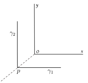
Figure 1. Angle is not continuous. The angle between $\gamma_{1}$ and $\gamma_{2}$ is $\pi/2$ while the angle between $\mathcal{O}x$ and $\mathcal{O}y$ is $\pi$.

A particularly useful property of $(T_{p}\mathcal{M},\mathbf{d}_{p})$ is that triangles in $T_{p}\mathcal{M}$ with one vertex at the apex are flat.

Lemma 1.23 (Lemma 3.6.15, [BBI01]).

Fix a $\operatorname{CAT}(\kappa)$ space $\mathcal{M}$. For $V,W\in T_{p}\mathcal{M}$ such that $\angle(V,W)<\pi$, let $U(s),s\in[0,1]$ be a geodesic of constant speed in $(T_{p}\mathcal{M},\mathbf{d}_{p})$ joining $V$ to $W$. Then $tU(s)$ for $s\in[0,1]$ is a geodesic from $tW$ to $tV$ for all $t\in[0,1]$. In particular, any triangle in $T_{p}\mathcal{M}$ with one vertex at the apex is flat.

Proof.

It suffices to show that, for $t,s\in[0,1]$,

$$\mathbf{d}_{p}(tV,tW)=\mathbf{d}_{p}\bigl{(}tV,tU(s)\bigr{)}+\mathbf{d}_{p}(tU(s),tW).$$

The above equality holds true for $t=1$ because $U(s)$ for $s\in[0,1]$ is a geodesic connecting $V$ and $W$. Thus

$$\mathbf{d}_{p}(V,W)=\mathbf{d}_{p}\bigl{(}V,U(s)\bigr{)}+\mathbf{d}_{p}\bigl{(}U(s),W\bigr{)}\text{ for }s\in[0,1].$$

We now deduce, from the conical metric (Definition 1.12), that

$$\mathbf{d}_{p}(tV,tW) =\sqrt{\lVert tV\rVert^{2}+\lVert tW\rVert^{2}-2t^{2}\lVert V\rVert\lVert W\rVert\cos\bigl{(}\angle(V,W)\bigr{)}}$$

$$=t\sqrt{\lVert V\rVert^{2}+\lVert W\rVert^{2}-2\lVert V\rVert\lVert W\rVert\cos\bigl{(}\angle(V,W)\bigr{)}}$$

$$=t\mathbf{d}_{p}(V,W).$$

Similarly, for $s\in[0,1],$

$$\mathbf{d}_{p}\bigl{(}tV,tU(s)\bigr{)}=t\mathbf{d}_{p}\bigl{(}V,U(s)\bigr{)}\quad\text{and}\quad\mathbf{d}_{p}\bigl{(}tU(s),tW\bigr{)}=t\mathbf{d}_{p}\bigl{(}U(s),W\bigr{)}.$$

Therefore

$$\mathbf{d}_{p}(tV,tW) =t\mathbf{d}_{p}(V,W)$$

$$=t\bigl{(}\mathbf{d}_{p}(V,U(s)\bigr{)}+\mathbf{d}_{p}\bigl{(}U(s),W)\bigr{)}$$

$$=\mathbf{d}_{p}\bigl{(}tV,tU(s)\bigr{)}+\mathbf{d}_{p}\bigl{(}tU(s),tW\bigr{)},$$

which completes the proof. ∎

This section concludes with two easy results that stand on their own as generally useful but also arise in the intended application of this theory to measures on smoothly stratified metric spaces; see [MMT23b, Lemma 2.29], for example.

Proposition 1.24.

If $\mathcal{M}$ is $\operatorname{CAT}(\kappa)$ and locally compact then $(T_{p}\mathcal{M},\mathbf{d}_{p})$ is $\operatorname{CAT}(0)$: it is complete space simply connected, and globally nonpositively curved (NPC).

Proof.

Because the metric $\mathbf{d}_{p}$ on $T_{p}\mathcal{M}$ is homogeneous (commutes with scaling), any triangle can be brought to a similar one in any neighborhood of the apex in $T_{p}\mathcal{M}$. Thus, $T_{p}\mathcal{M}$ is nonpositively curved in the global sense ([BBI01, Definition 4.6.6]). Due to local compactness, $T_{p}\mathcal{M}$ is complete since the space of directions is complete. Now invoke [BBI01, Remark 9.2.1] to conclude that $(T_{p}\mathcal{M},\mathbf{d}_{p})$ is simply connected and hence a global NPC space. ∎

Corollary 1.25.

If $\mathcal{M}$ is $\operatorname{CAT}(\kappa)$ and locally compact then $(S_{p}\mathcal{M},d_{s})$ is $\operatorname{CAT}(1)$.

Proof.

It follows from Proposition 1.24 that $(T_{p}\mathcal{M},\mathbf{d}_{p})$ is a $\operatorname{CAT}(0)$ space. As $(T_{p}\mathcal{M},\mathbf{d}_{p})$ is a Euclidean cone over $(S_{p}\mathcal{M},\mathbf{d}_{s})$, invoke [BBI01, Theorem 4.7.1] to conclude that $(S_{p}\mathcal{M},\mathbf{d}_{s})$ has curvature bounded above by $1$. ∎

2. Radial transport

Defining parallel transport on $(T_{p}\mathcal{M},\mathbf{d}_{p})$ for $\operatorname{CAT}(\kappa)$ space $\mathcal{M}$ is difficult in general. For a simple example, excise the open first quadrant of the plane $\mathbb{R}^{2}$ as in Figure 2; what results is a $\operatorname{CAT}(0)$ stratified space whose tangent cone at the origin does not compare with any tangent cones nearby. However, not all is lost: parallel rays are still defined on $\operatorname{CAT}(0)$ spaces. Hence limits of tangent cones can be taken upon approach to a singular point. This way of comparing tangent cones is enough to push the fluctuating cone through a dévissage process and hence compare $T_{p}\mathcal{M}$ to a vector space.

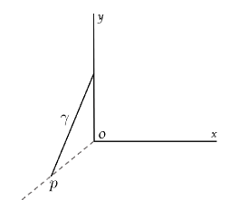
Figure 2. The plane with open first quadrant excised. The geodesic segment $\gamma$ cannot be extended indefinitely, so no ray is parallel to it.

The hypotheses for this section start with a $\operatorname{CAT}(\kappa)$ space $\mathcal{M}$ and its tangent cone $\mathcal{X}=T_{p}\mathcal{M}$, whose apex may be called $p$ but alternatively may be called $\mathcal{O}\in\nolinebreak\mathcal{X}$ to distinguish it from $p\in\mathcal{M}$.

Although parallel transport in $\mathcal{M}$ need not be well defined, only parallel transport on $T_{p}\mathcal{M}$ along geodesics starting from the apex $p$ is required for our CLT. (That explains the typical hypothesis $\mathcal{X}=T_{p}\mathcal{M}$ in this section.) This “radial transport” works because every triangle with a vertex at the cone point is flat by Lemma 1.23.

First recall some background on parallel lines and rays in $\operatorname{CAT}(0)$ spaces such as $\mathcal{X}$ from [BBI01, Chapter 9], where more details can be found.

Definition 2.1 (Lines).

A line in a $\operatorname{CAT}(0)$ space $\mathcal{X}$ is a unit-speed geodesic $\gamma:\mathbb{R}\to\mathcal{X}$ such that every closed subinterval of $\gamma$ is a shortest path in $\mathcal{X}$. A ray in $\mathcal{X}$ is a half-line geodesic $\gamma:[0,+\infty)\to\mathcal{X}$.

Definition 2.2 (Parallel lines).

In a $\operatorname{CAT}(0)$ space, two unit-speed lines or rays $\gamma_{1}(t)$ and $\gamma_{2}(t)$ are parallel, written $\gamma_{1}\parallel\gamma_{2}$, if the function $f(t)=\mathbf{d}\bigl{(}\gamma_{1}(t),\gamma_{2}(t)\bigr{)}$ is bounded.

Lemma 2.3 ([BBI01, Proposition 9.2.28]).

Fix a point $z$ in a $\operatorname{CAT}(0)$ space $\mathcal{X}$. For any ray $\gamma\bigl{(}[0,+\infty)\bigr{)}$ in $\mathcal{X}$ there exists a unique ray parallel to $\gamma$ starting at $z$.

Remark 2.4.

Fix a $\operatorname{CAT}(\kappa)$ space $\mathcal{M}$ and $\mathcal{X}=T_{p}\mathcal{M}$ with apex $\mathcal{O}$. Fix $z\in\mathcal{X}$ and a point $q\neq\mathcal{O}$ on the geodesic $\mathcal{O}z$ joining $\mathcal{O}$ to $z$. Suppose that $V_{z}$ is a vector in $T_{z}\mathcal{X}$ whose exponential $\exp_{z}V_{z}$ is defined. The triangle formed by $\mathcal{O}$, $z$, and $\exp_{z}V_{z}$ is flat by Lemma 1.23. Hence a unique point $v_{q}$ lies on the geodesic from $\mathcal{O}$ to $\exp_{z}V_{z}$ such that the geodesic segment $qw_{q}$ is parallel to $\exp_{z}V_{z}$ in the Euclidean sense; see Figure 3.

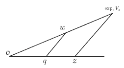
Figure 3. A Euclidean (flat) sector in $\mathcal{X}$ spanned by $\mathcal{O}z$ and $\mathcal{O}v_{z}$ where $v_{z}=\exp_{z}V_{z}$. For any non-apex $q$ on $\mathcal{O}z$, there is only one $v_{q}$ on $\mathcal{O}v_{z}$ such that $qv_{q}\parallel zv_{z}$ in the Euclidean sense.

Definition 2.5 (Parallel vectors).

The two vectors $V_{q}=\log_{q}v_{q}$ and $V_{z}$ in Remark 2.4 are parallel. More generally, if $\mathcal{X}=T_{p}\mathcal{M}$ with apex $\mathcal{O}$, and $q$ lies on the geodesic $\mathcal{O}z$ from $\mathcal{O}$ to $z$ in $\mathcal{X}$, then two nonzero vectors $V_{z}\in T_{z}\mathcal{X}$ and $V_{q}\in T_{q}\mathcal{X}$ are parallel if there exist $\varepsilon_{z}>0$ and $\varepsilon_{q}>0$ such that $\varepsilon_{z}V_{z}$ and $\varepsilon_{q}V_{q}$ are parallel.

Lemma 2.6.

Let $\mathcal{M}$ be $\operatorname{CAT}(\kappa)$ and $\mathcal{X}=T_{p}\mathcal{M}$ with apex $\mathcal{O}$. Fix $z\in\mathcal{X}$ and $q\in\mathcal{O}z$. Any nonzero vector $V_{z}\in T_{z}\mathcal{X}$ has a unique unit vector $V_{q}\in T_{q}\mathcal{X}$ parallel to $V_{z}$.

Proof.

The point $v_{q}$ in Remark 2.4 is unique. ∎

Definition 2.7 (Radial transport).

Let $\mathcal{M}$ be $\operatorname{CAT}(\kappa)$ and $\mathcal{X}=T_{p}\mathcal{M}$ with apex $\mathcal{O}$. Fix $z\in\mathcal{X}$ and $\mathcal{O}\neq q\in\mathcal{O}z$. For any unit vector $V_{z}\in T_{z}\mathcal{X}$ let $V_{q}$ be the unit vector in $T_{q}\mathcal{X}$ parallel to $V_{z}$ afforded by Lemma 2.6. The radial transport from $q$ to $z$ is

$$\mathfrak{p}_{q\to z}:T_{q}\mathcal{X} \to T_{z}\mathcal{X}$$

$$tV_{q} \mapsto tV_{z}\text{ for all }t\geq 0.$$

The inverse of $\mathfrak{p}_{q\to z}$ is the radial transport $\mathfrak{p}_{z\to q}=\mathfrak{p}_{q\to z}^{-1}$ (justified by Proposition 2.8).

Proposition 2.8.

Radial transport is an isometry: in Definition 2.7, $W_{z}=\mathfrak{p}_{q\to z}(W_{q})\Rightarrow$

$$\angle(V_{z},W_{z})=\angle(V_{q},W_{q}).$$

Proof.

Write $|xy|$ for the length of the geodesic segment from $x$ to $y$ when the space containing $x$ and $y$ is clear from context. Given $s\in(0,1)$ such that $s<|\mathcal{O}q|$, write

(2.1) $$v_{p}=\exp_{p}\bigl{(}{\textstyle\frac{|\mathcal{O}p|}{|\mathcal{O}z|}}sV_{p}\bigr{)}\ \text{ and }\ w_{p}=\exp_{p}\bigl{(}{\textstyle\frac{|\mathcal{O}p|}{|\mathcal{O}z|}}sW_{p}\bigr{)}$$

for $p\in\{q,z\}$; see Figure 4.

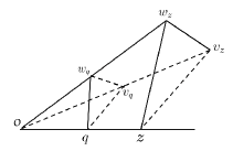
Figure 4. The same setup as in Figure 3 but with two flat sectors. Here $v_{q}w_{q}\parallel v_{z}w_{z}$.

If any of the points $w_{p}$ or $v_{p}$ for $p\in\{q,z\}$ lie in the geodesic through $\mathcal{O}$ and $z$, the condition $s<|\mathcal{O}q|$ ensures that those points lie in the ray $\{\exp_{\mathcal{O}}tz\}_{t\geq 0}$, so radial transport applies.

The six triangles $\triangle\mathcal{O}pv_{p}$, $\triangle\mathcal{O}pw_{p}$, and $\triangle\mathcal{O}v_{p}w_{p}$ for $p\in\{q,z\}$ are flat by Lemma 1.23. Since $qv_{q}\parallel zv_{z}$ and $qw_{q}\parallel zw_{z}$, with both length ratios being $\frac{|\mathcal{O}q|}{|\mathcal{O}z|}$ by construction,

$$\frac{|\mathcal{O}v_{q}|}{|\mathcal{O}v_{z}|}=\frac{|\mathcal{O}w_{q}|}{|\mathcal{O}w_{z}|}=\frac{|\mathcal{O}q|}{|\mathcal{O}z|}.$$

As $\triangle\mathcal{O}v_{z}w_{z}$ is also flat, it follows that $v_{q}w_{q}\parallel v_{z}w_{z}$ and that

$$\frac{|v_{q}w_{q}|}{|v_{z}w_{z}|}=\frac{|\mathcal{O}q|}{|\mathcal{O}z|}.$$

Hence the two triangles $\triangle qv_{q}w_{q}$ and $\triangle zv_{z}w_{z}$ are similar, so $\angle(qv_{q},qw_{q})=\angle(zv_{z},zw_{z})$ independent of $s$ in (2.1). Letting that $s$ converge to $0$ leads to the conclusion that $\angle(V_{q},W_{q})=\angle(V_{z},W_{z})$, as desired. ∎

Remark 2.9.

Proposition 2.8 and the definition of radial transport here differ from [MBH15, Theorem 2.11]. In particular, results stated in [MBH15, Theorem 2.11] rely on the definition, at the beginning of page 4 in that paper, that parallel rays $\gamma_{1}(t)$ and $\gamma_{2}(t)$ have constant, uniform distance; that is

$$\mathbf{d}\bigl{(}\gamma_{1}(t),\gamma_{2}(t)\bigr{)}=C$$

for some constant $C$. From this definition, [MBH15, Lemma 2.9] claims that given a ray $\gamma_{1}$ and a point $p$ there always exists a ray $\gamma_{2}$ starting from $p$ that is parallel to $\gamma_{2}$. However, a counterexample to this claim is depicted in Figure 5.

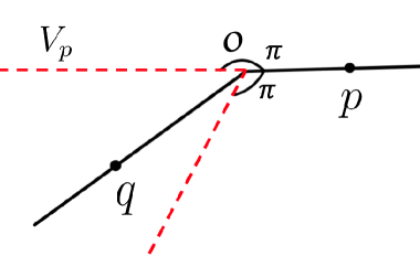
Figure 5. On a topological plane with isolated singularity of total angle $3\pi$, the red dashes are the boundary of the shadow of $\mathcal{O}p$. If $q$ is in the shadow and $V_{p}$ is the unit vector in the direction $p\mathcal{O}$ then there is no ray that starts from $q$ and is parallel to $V_{p}$ as defined in [MBH15].

Since the purpose of radial transport is to collapse by dévissage, the next goal is to extend radial transport to the case where the initial point is the apex $\mathcal{O}$.

Remark 2.10.

Let $\mathcal{M}$ be $\operatorname{CAT}(\kappa)$ and $\mathcal{X}=T_{p}\mathcal{M}$ with apex $\mathcal{O}$. Fix $z\in\mathcal{X}$. Suppose that $V\in T_{\mathcal{O}}\mathcal{X}$ is tangent to the cone point. The ray $\exp_{\mathcal{O}}tV$ is well defined for $t\in[0,\infty)$ since $\mathcal{O}$ is the apex. Lemma 2.3 produces a unique ray $\gamma\bigl{(}[0,\infty)\bigr{)}$ starting at $z$ and parallel to $\exp_{\mathcal{O}}tV$. As $\gamma\bigl{(}[0,\infty)\bigr{)}$ is a geodesic, it has a unit tangent $V_{z}\in T_{z}\mathcal{X}$ that is thought of as parallel to $V$. The precise definition follows.

Definition 2.11 (Parallel vectors, one at $\mathcal{O}$).

Let $\mathcal{M}$ be $\operatorname{CAT}(\kappa)$ and $\mathcal{X}=T_{p}\mathcal{M}$ with apex $\mathcal{O}$. Fix $z\in\mathcal{X}$. For any unit vector $V\in T_{\mathcal{O}}\mathcal{X}$, let $V_{z}\in T_{z}\mathcal{X}$ be the unique unit vector such that the ray $\exp_{\mathcal{O}}tV$ is parallel to the ray $\exp_{z}tV_{z}$. The vectors $tV$ and $tV_{z}$ are parallel, written $tV\parallel tV_{z}$, for all $t\in[0,\infty)$.

Definition 2.12 (Radial transport from $\mathcal{O}$).

Let $\mathcal{M}$ be $\operatorname{CAT}(\kappa)$ and $\mathcal{X}=T_{p}\mathcal{M}$ with apex $\mathcal{O}$. Fix $z\in\mathcal{X}$. The radial transport from $\mathcal{O}$ to $z$ is the map

$$\mathfrak{p}_{\mathcal{O}\to z}:T_{\mathcal{O}}\mathcal{X} \to T_{z}\mathcal{X}$$

$$tV \mapsto tV_{z}\text{ for all }t\geq 0$$

in which $tV\parallel tV_{z}$ as in Definition 2.11.

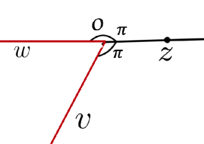
Figure 6. Radial transport from $\mathcal{O}$ to $z$ is not isometric. Both $v$ and $w$ are mapped to a vector in the direction from $z$ to $\mathcal{O}$.

Remark 2.13.

Transport from $T_{z}\mathcal{X}$ to $T_{\mathcal{O}}\mathcal{X}$ might not be possible because rays starting from $z$ may not extend indefinitely. This failure is related to Remark 2.14.

Remark 2.14.

Unlike radial transport between two non-apex points in Definition 2.7, radial transport $\mathfrak{p}_{\mathcal{O}\to z}$ from the apex $\mathcal{O}$ to a less singular point $z$ need not be an isometry. For example, if $V,W\in T_{\mathcal{O}}\mathcal{X}$ have $\angle(V,\log_{\mathcal{O}}z)=\angle(W,\log_{\mathcal{O}}z)=\pi$ (so $V$ and $W$ lie in the shadow of $z$; see Figure 6 and Definition 3.7), then $\mathfrak{p}_{\mathcal{O}\to z}V=\mathfrak{p}_{\mathcal{O}\to z}W$.

Remark 2.14 notwithstanding, not all is lost where the isometry is concerned; see Proposition 3.10. To explore how much isometry survives, another notion is required.

Definition 2.15 (Half-strip).

Let $\mathcal{M}$ be $\operatorname{CAT}(\kappa)$ and $\mathcal{X}=T_{p}\mathcal{M}$ with apex $\mathcal{O}$. Parallel rays $\gamma_{1},\gamma_{2}\subseteq\mathcal{X}$ span a convex flat half-strip if there are parallel rays $\zeta_{1},\zeta_{2}$ in $\mathbb{R}^{2}$ and an isometry $\iota$ that maps the convex hull of $\gamma_{1}$ and $\gamma_{2}$ in $\mathcal{X}$ to the convex hull of $\zeta_{1}$ and $\zeta_{2}$ in $\mathbb{R}^{2}$ satisfying $\zeta_{1}(t)=\iota\bigl{(}\gamma_{1}(t)\bigr{)}$ and $\zeta_{2}(t)=\iota\bigl{(}\gamma_{2}(t)\bigr{)}$ for all $t\in[0,\infty)$.

The exponentials in the following result exist because they occur in a conical space.

Proposition 2.16.

Let $\mathcal{M}$ be $\operatorname{CAT}(\kappa)$ and $\mathcal{X}=T_{p}\mathcal{M}$ with apex $\mathcal{O}$. Fix $z\in\mathcal{X}$ and a unit vector $V\in T_{\mathcal{O}}\mathcal{X}$. Set $V_{z}=\mathfrak{p}_{\mathcal{O}\to z}V\in T_{z}\mathcal{X}$. Then $\exp_{\mathcal{O}}tV$ and $\exp_{z}(tV_{z})$ for $t\in[0,\infty)$ span a convex flat half-strip (whose width can be $0$).

Proof.

It follows from the proof of [BBI01, Proposition 9.2.28] that the ray $\exp_{\mathcal{O}}tV$ is the limit of the geodesic from $\mathcal{O}$ to $\exp_{z}(tV_{z})$ as $t$ goes to infinity. In other words,

$$V=\lim_{t\to\infty}\frac{\log_{\mathcal{O}}\bigl{(}\exp_{z}(tV_{z})\bigr{)}}{\bigl{\|}\log_{\mathcal{O}}\bigl{(}\exp_{z}(tV_{z})\bigr{)}\bigr{\|}}.$$

On the other hand, invoke Lemma 1.23 again to see that the convex hull of $\mathcal{O}$ and the ray $\exp_{z}(tV_{z})$ is flat. Hence the convex hull of $\exp_{\mathcal{O}}tV$ and $\exp_{z}(tV_{z})$ is also flat. ∎

3. Limit tangent spaces and limit logarithm maps

Radial transport compares tangent cones as they approach the apex $\mathcal{O}$ along a geodesic. Proposition 2.8 says that those tangent cones are isometric via radial transport. It is therefore natural to identify them in the limit, as follows.

Definition 3.1 (Limit tangent cone).

Let $\mathcal{M}$ be $\operatorname{CAT}(\kappa)$ and $\mathcal{X}=T_{p}\mathcal{M}$ with apex $\mathcal{O}$. Fix $Z\in T_{\mathcal{O}}\mathcal{X}$. For $q,q^{\prime}\in\mathcal{O}z$ between $\mathcal{O}$ and $z=\exp_{\mathcal{O}}Z$, radial transport $\mathfrak{p}_{q\to q^{\prime}}$ identifies $T_{q}\mathcal{X}$ with $T_{q^{\prime}}\mathcal{X}$. The limit tangent cone along $Z$ is the direct limit

$$\smash{\makebox[0.0pt][l]{$T$}\raisebox{6.02773pt}{\scalebox{1.1}[0.5]{${}^{\rightarrow\!\!}$}}}_{Z}\mathcal{X}=\varinjlim_{q\in\mathcal{O}z}T_{q}\mathcal{X}.$$

Write $\smash{\makebox[0.0pt][l]{$S$}\raisebox{6.02773pt}{\scalebox{1.1}[0.5]{${}^{\rightarrow\!\!}$}}}_{Z}\mathcal{X}$ for the unit sphere around the apex in $\smash{\makebox[0.0pt][l]{$T$}\raisebox{6.02773pt}{\scalebox{1.1}[0.5]{${}^{\rightarrow\!\!}$}}}_{Z}\mathcal{X}$.

Remark 3.2.

The direct limit here is an algebraic or categorical notion rather than an analytic one; see [Lan02, Chapter III.10]. An element of $\smash{\makebox[0.0pt][l]{$T$}\raisebox{6.02773pt}{\scalebox{1.1}[0.5]{${}^{\rightarrow\!\!}$}}}_{Z}\mathcal{X}$ is represented by a tangent vector in $T_{q}\mathcal{X}$ at a point beteween $\mathcal{O}$ and $z$, and two such vectors—at different points—represent the same limit tangent element if they are parallel transports of each other. The direct limit allows radial transport from the apex (Definition 2.12) to be viewed as comparing tangent data at $\mathcal{O}$ to tangent data infinitesimally near $\mathcal{O}$ along the given direction $Z$. In applications to smoothly stratified spaces $\mathcal{M}$ [MMT23b], the limit tangent space $\smash{\makebox[0.0pt][l]{$T$}\raisebox{6.02773pt}{\scalebox{1.1}[0.5]{${}^{\rightarrow\!\!}$}}}_{Z}\mathcal{X}$ is automatically less singular than $\mathcal{X}=T_{p}\mathcal{M}$ itself, in the precise sense that the codimension of the singularity decreases upon taking limit tangent spaces; see [MMT23b, Proposition 4.18.2]. Indeed, this is a key motivation for defining limit tangent spaces.

Remark 3.3.

Barden and Le define boundary limits of translated logarithm maps in orthant spaces [BL18, Theorem 2], which accomplish what limit log maps do here. Translation can substitute in orthant spaces for the more general but weaker radial transport because orthant spaces are glued from pieces of Euclidean spaces [MOP15].

The exponentials in the following result exist because they occur in a conical space.

Definition 3.4 (Limit log map).

Let $\mathcal{M}$ be $\operatorname{CAT}(\kappa)$ and $\mathcal{X}=T_{p}\mathcal{M}$ with apex $\mathcal{O}$. Fix $Z\in T_{\mathcal{O}}\mathcal{X}$. For any $V\in T_{\mathcal{O}}\mathcal{X}$ and any $q\in\mathcal{O}z$ between $\mathcal{O}$ and $z=\exp_{\mathcal{O}}Z$, write $V_{q}=\mathfrak{p}_{\mathcal{O}\to q}V$. Let $V_{Z}$ be the image of $V_{q}$ (for any $q\neq\mathcal{O}$) in the limit tangent space $\smash{\makebox[0.0pt][l]{$T$}\raisebox{6.02773pt}{\scalebox{1.1}[0.5]{${}^{\rightarrow\!\!}$}}}_{Z}\mathcal{X}$. The limit log map along $Z$ is

$$\mathcal{L}_{Z}:T_{\mathcal{O}}\mathcal{X} \to\smash{\makebox[0.0pt][l]{$T$}\raisebox{6.02773pt}{\scalebox{1.1}[0.5]{${}^{\rightarrow\!\!}$}}}_{Z}\mathcal{X}$$

$$tV \mapsto tV_{Z}\text{ for all }t\geq 0.$$

Remark 3.5.

The usual log map at a point $p$ in a $\operatorname{CAT}(\kappa)$ space $\mathcal{M}$ takes each point $p\in\mathcal{M}$ to the tangent at $p$ of the geodesic aimed at the terminus $p$ as it exits the initial point $p$. In contrast, the limit log map at $p$ in the direction $Z$ reflects what happens when each point $p$ goes to the tangent of the geodesic aimed at the terminus $p$ as it exits an initial point $p^{\prime}_{Z}$ that is infinitesimally near $p$ along $Z$. The limit log map is more accurately the derivative of this mapping, in that it takes the tangent vector pointing from $p$ toward $p$ to a tangent vector at $p^{\prime}_{Z}$. This information is recorded at $p$ itself, rather than at $p^{\prime}_{Z}$, via the direct limit in Definition 3.1.

Remark 3.6.

The limit log map was called the folding map on a hyperbolic topological plane with isolated singularity [HMMN15] or on an open book [HHL⁺13] because the limit log map along a direction $Z$ collapses rays whose directions are “beyond opposite” to $Z$. The general version is made precise in the next Definition and Remark.

Definition 3.7 (Shadow).

Let $\mathcal{M}$ be $\operatorname{CAT}(\kappa)$ and $\mathcal{X}=T_{p}\mathcal{M}$ with apex $\mathcal{O}$. The shadow of a tangent vector $Z\in T_{\mathcal{O}}\mathcal{X}$ is the set $\mathcal{I}(Z)$ of nonzero vectors that form an angle of $\pi$ with $Z$:

$$\mathcal{I}(Z)=\{V\in T_{\mathcal{O}}\mathcal{X}\mid\angle(V,Z)=\pi\}.$$

Remark 3.8.

When $V$ lies in the shadow of $Z$, the ray through $Z$ parallel to $\exp_{\mathcal{O}}tV$ passes through $\mathcal{O}$ itself. Hence, by Definition 3.4 (see also Definitions 2.11 and 2.12), $\mathcal{L}_{Z}(V)$ is a scalar multiple of the vector $\log_{Z}\mathcal{O}$ that points from $Z$ directly toward $\mathcal{O}$. This vector arises numerous times and can be written in various ways, such as

$$\log_{Z}\mathcal{O}=-\mathcal{L}_{Z}(Z)=-\mathfrak{p}_{\mathcal{O}\to z}(Z)$$

for $z=\exp_{\mathcal{O}}Z$, all expressing that this vector is the unit tangent at $Z$ to the ray $Z\mathcal{O}$ traversed backward along the ray $\mathcal{O}Z$. The scalar in question is $\|\mathcal{L}_{Z}(V)\|/\|\mathord{-}\mathcal{L}_{Z}(Z)\|$. In particular, if a sequence of vectors in $T_{\mathcal{O}}\mathcal{X}$ converges to a vector in the shadow of $Z$, then the sequence of images under the limit log map converges to this same vector:

$$\frac{\mathcal{L}_{Z}V}{\|\mathcal{L}_{Z}V\|}\to\frac{-\mathcal{L}_{Z}Z}{\|\mathcal{L}_{Z}Z\|}\ \text{ as }\ V\to\mathcal{I}(Z).$$

The next result generalizes this observation that after taking the limit log map along $Z$, the shadow $\mathcal{I}(Z)$ becomes the exact opposite vector of $Z$.

Proposition 3.9.

Let $\mathcal{M}$ be $\operatorname{CAT}(\kappa)$ and $\mathcal{X}=T_{p}\mathcal{M}$ with apex $\mathcal{O}$. Fix $Z\in\nolinebreak\!T_{\mathcal{O}}\mathcal{X}$. For any $W_{Z}\in\smash{\makebox[0.0pt][l]{$T$}\raisebox{6.02773pt}{\scalebox{1.1}[0.5]{${}^{\rightarrow\!\!}$}}}_{Z}\mathcal{X}$,

$$\angle\bigl{(}\mathcal{L}_{Z}(Z),W_{Z}\bigr{)}+\angle\bigl{(}W_{Z},-\mathcal{L}_{Z}(Z)\bigr{)}=\angle\bigl{(}\mathcal{L}_{Z}(Z),-\mathcal{L}_{Z}(Z)\bigr{)}=\pi.$$

Proof.

Set $z=\exp_{\mathcal{O}}Z\in\mathcal{X}$. By definition of $-\mathfrak{p}_{\mathcal{O}\to z}(Z)$ in Remark 3.8,

$$\angle(\mathfrak{p}_{\mathcal{O}\to z}Z,-\mathfrak{p}_{\mathcal{O}\to z}Z)=\pi.$$

By Lemma 1.23, the convex hull of $\mathcal{O}W_{Z}$ and $\mathcal{O}z$ is flat, so

$$\angle(\mathfrak{p}_{\mathcal{O}\to z}Z,W_{Z})+\angle(W_{Z},-\mathfrak{p}_{\mathcal{O}\to z}Z)=\angle(\mathfrak{p}_{\mathcal{O}\to z}Z,-\mathfrak{p}_{\mathcal{O}\to z}Z)=\pi,$$

and the desired result follows. ∎

Although radial transport from $\mathcal{O}$ to $z$ is not an isometry, it is close to being one, in the sense that it retains isometric properties away from the shadow.

Proposition 3.10.

Let $\mathcal{M}$ be $\operatorname{CAT}(\kappa)$ and $\mathcal{X}=T_{p}\mathcal{M}$ with apex $\mathcal{O}$. Fix unit vectors $V,W,Z\in T_{\mathcal{O}}\mathcal{X}$ with $\angle(V,W)<\pi$ such that the geodesic $VW$ in $T_{\mathcal{O}}\mathcal{X}$ does not intersect the shadow $\mathcal{I}(Z)$. Let $z=\exp_{\mathcal{O}}Z$ and $U_{z}=\mathfrak{p}_{\mathcal{O}\to z}U$ for $U\in\{V,W\}$. Then

$$\angle(V,W)=\angle(V_{z},W_{z}),$$

and at the level of geodesics, $V_{z}W_{z}=\mathfrak{p}_{\mathcal{O}\to z}(VW)$.

Proof.

Given $r\in(0,1]$, write

$$v=\exp_{\mathcal{O}}rV,\ \ \ \ \,v_{z}=\exp_{z}rV_{z},$$

$$w=\exp_{\mathcal{O}}rW, \ \ \ w_{z}=\exp_{z}rW_{z}.$$

It follows from Proposition 2.16 that the rays $\exp_{\mathcal{O}}(tV)$ and $\exp_{z}tV_{z}$ span a convex flat half-strip. Hence $\mathcal{O},v,V_{z},z$ constitute the vertices of a parallelogram (in $\mathbb{R}^{2}$). Similarly, $\mathcal{O},w,W_{z},z$ make a parallelogram (see Figure 7).

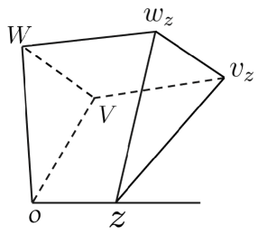
Figure 7.

Thus as $z$ approaches $\mathcal{O}$ along the geodesic $\exp_{\mathcal{O}}tZ$, the points $v_{z}$ and $w_{z}$ converge to $v$ and $w$, respectively.

Since the geodesic $VW$ in $T_{\mathcal{O}}\mathcal{X}$ does not intersect $\mathcal{I}(Z)$, the geodesic $v_{z}w_{z}$ does not intersect $\mathcal{O}z$ as $z\to\mathcal{O}$. Therefore the setup used to prove Proposition 2.8 (depicted in Figure 4) is valid for any choice of lengths for $\mathcal{O}z$ and $\mathcal{O}q$, even if the parameter $s$ there grows arbitrarily large. Thus the angle $\angle(V_{z},W_{z})$ and chordal distance $\mathbf{d}_{\mathcal{O}}(v_{z},w_{z})$ from $v_{z}$ to $w_{z}$ remain constant as $z$ converges to $\mathcal{O}$ along $\exp_{\mathcal{O}}tZ$, so $\mathbf{d}_{\mathcal{O}}(v_{z},w_{z})=\mathbf{d}_{\mathcal{O}}(v,w)$. Letting $r\to 0$ leads to the desired conclusion that $\angle(V,W)=\angle(V_{z},W_{z})$. ∎

Corollary 3.11.

Let $\mathcal{M}$ be $\operatorname{CAT}(\kappa)$ and $\mathcal{X}=T_{p}\mathcal{M}$ with apex $\mathcal{O}$. Fix unit vectors $V,W,Z\in T_{\mathcal{O}}\mathcal{X}$ such that the geodesic in $T_{\mathcal{O}}\mathcal{X}$ from $V$ to $W$ does not intersect the shadow $\mathcal{I}(Z)$ of $Z$. Then

$$\angle(V,W)=\angle(\mathcal{L}_{Z}V,\mathcal{L}_{Z}W)\quad\text{and}\quad\mathcal{L}_{Z}V\,\mathcal{L}_{Z}W=\mathcal{L}_{Z}(VW).$$

Proof.

Combine Proposition 3.10 with the Definition 3.4 of limit log map $\mathcal{L}_{Z}$. ∎

Corollary 3.12.

In the setting of Definition 3.4, the limit log map $\mathcal{L}_{Z}$ is continuous.

Proof.

It follows from Remark 3.8 when $W$ is in the interior of $\mathcal{I}(Z)$ and Proposition 3.10 when $W\notin\mathcal{I}(Z)$ that

$$\lim_{V\to W}\mathcal{L}_{Z}W=\mathcal{L}_{Z}W.$$

It remains to show that, for $W$ in the boundary of $\mathcal{I}(Z)$,

$$\lim_{V\to W,V\notin\mathcal{I}(Z)}\mathcal{L}_{Z}V=\mathcal{L}_{Z}W.$$

That is equivalent to

$$\lim_{V\to W,V\notin\mathcal{I}(Z)}\mathfrak{p}_{\mathcal{O}\to z}V=\mathfrak{p}_{\mathcal{O}\to z}W.$$

The point, to this end, is that when the unit vector $V\in T_{\mathcal{O}}\mathcal{X}$ approaches $\mathcal{I}(Z)$ in the proof of Proposition 2.16, the width of the flat half-strip spanned by $\exp_{\mathcal{O}}(tV)$ and $\exp_{Z}(t\mathfrak{p}_{\mathcal{O}\to z}V)$ decreases to $0$. If $\|V\|\neq 1$ then rescale. ∎

Corollary 3.13.

Fix $Z\in T_{\mathcal{O}}\mathcal{X}$, where $\mathcal{X}=T_{p}\mathcal{M}$ and $\mathcal{M}$ is $\operatorname{CAT}(\kappa)$. For all $V\!\in\nolinebreak\!T_{p}\mathcal{M}$,

$$\angle(V,Z)=\angle(\mathcal{L}_{Z}V,\mathcal{L}_{Z}Z).$$

Proof.

Either $V$ lies in the shadow $\mathcal{I}(Z)$, so both angles are $\pi$ by Remark 3.8, or else $\angle(Z,V)<\pi$, in which case use Proposition 3.10. ∎

Proposition 3.14.

Let $\mathcal{M}$ be $\operatorname{CAT}(\kappa)$ and $\mathcal{X}=T_{p}\mathcal{M}$ with apex $\mathcal{O}$. The limit log map is a contraction: if $\mathcal{X}=T_{p}\mathcal{M}$ and $Z\in\nolinebreak T_{\mathcal{O}}\mathcal{X}$ then

$$\angle(\mathcal{L}_{Z}V,\mathcal{L}_{Z}W)\leq\angle(V,W)$$

for any $V,W\in\mathcal{X}$.

Proof.

First observe that Proposition 3.10 remains true if one of the endpoints of the geodesic $VW$ lies in the shadow $\mathcal{I}(Z)$ but $VW$ is otherwise disjoint from $\mathcal{I}(Z)$, by using continuity in Corollary 3.12 to approach that endpoint from $VW\setminus\mathcal{I}(Z)$.

If $VW$ never enters the shadow, then the desired result is subsumed by Proposition 3.10. On the other hand, if $V$ and $W$ are unit vectors and $VW$ enters the shadow, then so does the shortest path $\gamma$ joining $V$ to $W$ in the unit tangent sphere. The length of $\gamma$ is $\angle(V,W)$ by definition. But the limit log map takes the first and last shadow points in $\gamma$ to the same point, namely $-\mathcal{L}_{Z}Z$, by Remark 3.8 (or Proposition 3.9, if that is preferred). Therefore, although the limit log map preserves the lengths of the initial and terminal segments of $\gamma$, which occur before entering $\mathcal{I}(Z)$ and after its final exit, the rest of $\mathcal{L}_{Z}(\gamma)$ is shortcut by remaining at $-\mathcal{L}_{Z}Z$. ∎

Continuity allows the hypothesis of Corollary 3.11 to be weakened to allow the geodesic from $V$ to $W$ to meet the shadow $\mathcal{I}(Z)$ at exactly one point, as in Figure 8.

Figure 8. Geodesic $VW$ meets the shadow $\mathcal{I}(Z)$ at exactly one point.

Proposition 3.15.

Let $\mathcal{M}$ be $\operatorname{CAT}(\kappa)$ and $\mathcal{X}=T_{p}\mathcal{M}$. For unit vectors $V,W,Z\in T_{\mathcal{O}}\mathcal{X}$ such that every shortest path from $V$ to $W$ in $T_{\mathcal{O}}\mathcal{X}$ meets $\mathcal{I}(Z)$ at exactly one point,

$$\mathbf{d}_{\mathcal{O}}(V,W)=\mathbf{d}_{Z}(\mathcal{L}_{Z}V,\mathcal{L}_{Z}W)\quad\text{and}\quad\mathcal{L}_{Z}V\,\mathcal{L}_{Z}W=\mathcal{L}_{Z}(VW),$$

where $\mathbf{d}_{Z}$ is the conical metric on $\smash{\makebox[0.0pt][l]{$T$}\raisebox{6.02773pt}{\scalebox{1.1}[0.5]{${}^{\rightarrow\!\!}$}}}_{Z}\mathcal{X}$ from Definition 1.12 applied to Definition 3.1.

Proof.

Let $Y=VW\cap\mathcal{I}(Z)$ be the single intersection point. The result is true if $Y=V$ or $Y=W$ by the first paragraph of the proof of Proposition 3.14. So break $VW$ into two pieces: $VW=VY\cup YW$ with $Y\not\in\{V,W\}$. Similar to the proof of Proposition 3.10, write $z=\exp_{O}Z$ and $U_{z}=\mathfrak{p}_{\mathcal{O}\to z}U$ for $U\in T_{\mathcal{O}}\mathcal{X}$, with

$$v=\exp_{\mathcal{O}}V,\ \ \ \ \,v_{z}=\exp_{z}V_{z},$$

$$w=\exp_{\mathcal{O}}W, \ \ \ w_{z}=\exp_{z}W_{z}.$$

$$y=\exp_{\mathcal{O}}Y,\ \ \ \ \,y_{z}=\exp_{z}Y_{z}.$$

Since $Y\not\in\{V,W\}$ is the only intersection between $VW$ and the shadow, $\angle(V,Z)<\nolinebreak\pi$ and $\angle(W,Z)<\pi$. Applying the setup from the proof of Proposition 3.10 (see Figure 7) and continuity of $\mathcal{L}_{Z}$, the parallelogram $\mathcal{O}zw_{z}w\subseteq\mathcal{X}$ expands to a closed half-plane $H_{W}$—isometric to a half-plane in $\mathbb{R}^{2}$, with boundary line spanned by $\mathcal{O}z$—that contains the ray $\mathcal{O}y$. Similarly, $\mathcal{O}zv_{z}v$ expands to a closed half-plane $H_{V}$. Then $\mathcal{L}_{Z}(UY)=U_{z}Y_{z}$ for $U\in\{V,W\}$ by the first paragraph of the proof of Proposition 3.14 again. The goal is to show that $|VW|=|V_{z}W_{z}|$, or equivalenty $|vw|=|v_{z}w_{z}|$, by the isometry $\exp_{\mathcal{O}}:\mathcal{X}\to T_{\mathcal{O}}\mathcal{X}$.

For $U\in\{V,W\}$ the half-plane $H_{U}$ contains a ray $R_{U}$ from $\mathcal{O}$ parallel to $YU$. Parallel transport $\mathfrak{p}_{\mathcal{O}\to y}$ demonstrates, by contraction in Proposition 3.14, that $\angle(R_{V},R_{W})\geq\angle(YV,YW)=\pi$, and hence $\angle(R_{V},R_{W})=\pi$. For $U\in\{V,W\}$ Let

$$U^{\prime}=R_{U}\cap U_{z}U.$$

Then $\angle(R_{V},R_{W})=\pi$ means $\angle(\mathcal{O}V^{\prime},\mathcal{O}W^{\prime})=\pi$ and

$$|V^{\prime}W^{\prime}|=\lVert V^{\prime}\rVert+\lVert W^{\prime}\rVert=|VY|+|YW|=|VW|.$$

Exponentiating at $\mathcal{O}$ yields $|v^{\prime}w^{\prime}|=|vw|$, so it suffices to show $|v^{\prime}w^{\prime}|=|v_{z}w_{z}|$.

For $\varepsilon>0$, let $v^{\prime}(\varepsilon)=\exp_{\mathcal{O}}\bigl{(}V^{\prime}(\varepsilon)\bigr{)}$ be a point at distance $\varepsilon$ from $v^{\prime}$ along the segment $v^{\prime}v_{z}$ in $\mathcal{X}$. The ray $R_{v}^{\varepsilon}$ from $\mathcal{O}$ through $v^{\prime}(\varepsilon)$ has angle $\angle(R_{v}^{\varepsilon},R_{w})<\pi$ with the ray $R_{w}=\exp_{\mathcal{O}}(R_{W})$. By Lemma 1.23 the convex hull of $R_{v}^{\varepsilon}$ and $R_{w}$ is a flat sector containing $w^{\prime}$, $w_{z}$, $v_{z}$, $v^{\prime}(\varepsilon)$, and $v_{z}(\varepsilon)=\exp_{z}\bigl{(}\mathfrak{p}_{\mathcal{O}\to z}V^{\prime}(\varepsilon)\bigr{)}$. Elementary geometry in this flat sector, using the parallelograms defined earlier, shows that $|v^{\prime}(\varepsilon)w^{\prime}|=|v_{z}(\varepsilon)w_{z}|$ for all $\varepsilon>0$. Letting $\varepsilon\to 0$ shows that $|v^{\prime}w^{\prime}|=|v_{z}w_{z}|$, as desired. ∎

Remark 3.16.

Proposition 3.15 is the strongest result possible by the argument that ends the proof of Proposition 3.14. The proof of Proposition 3.15, if carried out to its logical end, actually shows that the union of the half-planes $H_{V}$ and $H_{W}$ is an isometric copy of $\mathbb{R}^{2}$ inside of $\mathcal{X}$.

A rephrasing of Proposition 3.15 is the main result of the paper. It is one of the geometric drivers of central limit theory for measures on smoothly stratified metric spaces [MMT23b, Corollary 2.30].

Theorem 3.17.

Let $\mathcal{M}$ be $\operatorname{CAT}(\kappa)$ and $\mathcal{X}=T_{p}\mathcal{M}$. If $Z\in T_{\mathcal{O}}\mathcal{X}$ and $\mathcal{K}\subseteq T_{p}\mathcal{M}$ is a geodesically convex subcone containing at most one ray in the shadow $\mathcal{I}(Z)$, then the restriction $\mathcal{L}_{Z}|_{\mathcal{K}}:\mathcal{K}\to\mathcal{L}_{Z}(\mathcal{K})$ of the limit log map along $Z$ is an isometry onto its image.

Proof.

This is a direct consequence of Proposition 3.15. ∎

Remark 3.18.

Theorem 3.17 summarizes the limit log map $\mathcal{L}_{Z}$ the following way: $\mathcal{L}_{Z}$ collapses the shadow $\mathcal{I}(Z)$ to a single ray (Remark 3.8) while preserving the rest of $\mathcal{X}=T_{p}\mathcal{M}$ isometrically. Of course, any part of any geodesic that passes through the shadow collapses to a segement along the ray that is the collapsed image under $\mathcal{L}_{Z}$ of the shadow, but all geodesics otherwise maintain their integrity.

A simple consequence of Theorem 3.17 is generally useful and arises while manufacturing Gaussian-distributed vectors on the tangent cone of a smoothly stratified $\operatorname{CAT}(\kappa)$ space $\mathcal{M}$ [MMT23d, Section 6.1].

Corollary 3.19.

Let $\mathcal{M}$ be $\operatorname{CAT}(\kappa)$ and $\mathcal{X}=T_{p}\mathcal{M}$. If $Z\in T_{\mathcal{O}}\mathcal{X}$ then the limit log along $Z$ is a proper mapping.

Proof.

Limit log preserves distance from the apex by Theorem 3.17 (see Remark 3.18) and $\mathcal{M}$ is locally compact. ∎

The final less elementary consequence of Theorem 3.17 is key to preservation of fluctuating cones under limit log maps in subsequent work [MMT23b, Corollary 2.27]. It requires a simple definition.

Definition 3.20 (Hull).

Given a subset $\mathcal{S}\subseteq\mathcal{X}$ of a $\operatorname{CAT}(0)$ conical space $\mathcal{X}$, the hull of $\mathcal{S}$ is the smallest geodesically convex cone $\operatorname{hull}\mathcal{S}\subseteq\mathcal{X}$ containing $\mathcal{S}$.

Corollary 3.21.

Let $\mathcal{M}$ be $\operatorname{CAT}(\kappa)$ and $\mathcal{X}=T_{p}\mathcal{M}$. For any $Z\in T_{\mathcal{O}}\mathcal{X}$, taking limit log along $Z$ subcommutes with taking convex cones: for any subset $\mathcal{S}\subseteq\mathcal{X}$,

$$\mathcal{L}_{Z}(\operatorname{hull}\mathcal{S})\subseteq\operatorname{hull}\mathcal{L}_{Z}(\mathcal{S}).$$

Proof.

If $\operatorname{hull}(\mathcal{L}_{Z}\mathcal{S})$ contains no positive-length vector in $\mathcal{L}_{Z}\bigl{(}\mathcal{I}(Z)\bigr{)}$, then $\operatorname{hull}\mathcal{S}$ itself contains no positive-length vector in the shadow $\mathcal{I}(Z)$, because the lift of any shortest path not meeting $\mathcal{I}(Z)$ is a shortest path. Indeed, by Theorem 3.17 the preimage under $\mathcal{L}_{Z}$ of any shortest path not meeting $\mathcal{I}(Z)$ is a candidate geodesic between the preimage endpoints whose length equals the distance between the preimage endpoints, because limit log is a contraction by Proposition 3.14.

This reduces the question to the case where $\operatorname{hull}(\mathcal{L}_{Z}\mathcal{S})$ contains a positive-length vector in $\mathcal{L}_{Z}\bigl{(}\mathcal{I}(Z)\bigr{)}$. Let $\mathcal{S}^{\prime}$ be the union of all shortest paths in $\mathcal{X}$ between pairs of points of $\mathcal{S}$. Iterating if necessary, it suffices to prove $\mathcal{L}_{Z}(\mathcal{S}^{\prime})\subseteq\operatorname{hull}\mathcal{L}_{Z}(\mathcal{S})$. Suppose that $pq$ is a shortest path in $\mathcal{X}$ between $p\in\mathcal{S}$ and $q\in\mathcal{S}$. Then $pq$ breaks into a union of closed shortest paths each either contained in $\mathcal{I}(Z)$ or having at most one endpoint in $\mathcal{I}(Z)$. By Theorem 3.17, applying $\mathcal{L}_{Z}$ to each of these geodesic segments yields either a segment in $\mathcal{L}_{Z}\bigl{(}\mathcal{I}(Z)\bigr{)}$, which is contained in $\operatorname{hull}\mathcal{L}_{Z}(\mathcal{S})$ by hypothesis, or a shortest path from a point of $\mathcal{L}_{Z}(\mathcal{S})$ to $\mathcal{L}_{Z}\bigl{(}\mathcal{I}(Z)\bigr{)}$, which is also contained in $\operatorname{hull}\mathcal{L}_{Z}(\mathcal{S})$. ∎

References

- [BBI01] Dmitri Burago, Yuri Burago, and Sergei Ivanov, A course in metric geometry, volume 33, American Mathematical Soc., 2001.
- [BHV01] Louis J Billera, Susan P Holmes, and Karen Vogtmann, Geometry of the space of phylogenetic trees, Advances in Applied Mathematics 27 (2001), no. 4, 733–767.
- [BL18] Dennis Barden and Huiling Le, The logarithm map, its limits and Fréchet means in orthant spaces, Proceedings of the Londong Mathematical Society (3) 117 (2018), no. 4, 751–789.
- [BLO13] Dennis Barden, Huiling Le, and Megan Owen, Central limit theorems for Fréchet means in the space of phylogenetic trees, Electronic J. of Probability 18 (2013), no. 25, 25 pp.
- [BLO18] Dennis Barden, Huiling Le, and Megan Owen, Limiting behaviour of Fréchet means in the space of phylogenetic trees, Annals of the Institute of Statistical Mathematics 70 (2013), no. 1, 99–129.
- [BP03] Rabi Bhattacharya and Vic Patrangenaru, Large sample theory of intrinsic and extrinsic sample means on manifolds: I, Annals of Statistics 31 (2003), no. 1, 1–29.
- [BP05] Rabi Bhattacharya and Vic Patrangenaru, Large sample theory of intrinsic and extrinsic sample means on manifolds: II, Annals of Statistics 33 (2005), no. 3, 1225–1259.
- [BP23] Authors: Blanche Buet and Xavier Pennec, Flagfolds, preprint. arXiv:math.CA/2305.10583
- [FL+13] Aasa Feragen, Pechin Lo, Marleen de Bruijne, Mads Nielsen, and Fran cois Lauze, Toward a theory of statistical tree-shape analysis, IEEE Trans. Pattern Anal. Mach. Intell., 35 (2013), no. 8, 2008–2021.
- [GJS17] David Groisser, Sungkyu Jung, and Armin Schwartzman, Geometric foundations for scaling-rotation statistics on symmetric positive definite matrices: minimal smooth scaling-rotation curves in low dimensions, Electron. J. Stat. 11 (2017), no. 1, 1092–1159.
- [HHL+13] Thomas Hotz, Stephan Huckemann, Huiling Le, J.S. Marron, Jonathan C. Mattingly, Ezra Miller, James Nolen, Megan Owen, Vic Patrangenaru, and Sean Skwerer, Sticky central limit theorems on open books, Annals of Applied Probability 23 (2013), no. 6, 2238–2258.
- [HMMN15] Stephan Huckemann, Jonathan Mattingly, Ezra Miller, and James Nolen, Sticky central limit theorems at isolated hyperbolic planar singularities, Electronic Journal of Probability 20 (2015), 1–34.
- [Hol03] Susan Holmes, Statistics for phylogenetic trees, Theor. Popul. Bio. 63 (2003), no. 1, 17–32.
- [HTDL13] Richard Hartley, Jochen Trumpf, Yuchao Dai, and Hongdong Li, Rotation averaging, International journal of computer vision 103 (2013), no. 3, 267–305.
- [KBCL99] David G. Kendall, Dennis Barden, Thomas K. Carne, and Huiling Le, Shape and Shape Theory, Wiley Series in Probability and Statistics, Wiley & Sons, Ltd., Chichester, 1999.
- [Lan02] Serge Lang, Algebra. Revised third edition, Graduate Texts in Mathematics, vol. 211, Springer, 2002.
- [Le01] Huiling Le, Locating Fréchet means with application to shape spaces, Advances in Applied Probability 33 (2001), no. 2, 324–338.
- [LGNH21] Jonas Lueg, Maryam Garba, Tom Nye, and Stephan Huckemann, Wald space for phylogenetic trees, in Geometric Sci. of Inform., Lect. Notes in Comp. Sci. 12829 (2021), 710–717.
- [LSTY17] Bo Lin, Bernd Sturmfels, Xiaoxian Tang, and Ruriko Yoshida, Convexity in tree spaces, SIAM J. Discrete Math. 31 (2017), no. 3, 2015–2038.
- [MBH15] Mina Movahedi, Daryoush Behmardi, and Seyedehsomayeh Hosseini, On the density theorem for the subdifferential of convex functions on Hadamard spaces, Pacific Journal of Mathematics 276 (2015), no. 2, 437–447.
- [MMT23b] Jonathan Mattingly, Ezra Miller, and Do Tran, Geometry of measures on smoothly stratified metric spaces, preprint, 2023.
- [MMT23c] Jonathan Mattingly, Ezra Miller, and Do Tran, A central limit theorem for random tangent fields on stratified spaces, preprint, 2023.
- [MMT23d] Jonathan Mattingly, Ezra Miller, and Do Tran, Central limit theorems for Fréchet means on stratified spaces, preprint, 2023.
- [MOP15] Ezra Miller, Megan Owen, and Scott Provan, Polyhedral computational geometry for averaging metric phylogenetic trees, Advances in Applied Math. 15 (2015), 51–91. doi: 10.1016/j.aam.2015.04.002
- [PSD00] Jonathan K Pritchard, Matthew Stephens, and Peter Donnelly, Inference of population structure using multilocus genotype data, Genetics 155 (2000), no. 2, 945–959.
- [PSF20] Xavier Pennec, Stefan Sommer, and Tom Fletcher (eds.), Riemannian geometric statistics in medical image analysis, Acad. Press, 2020. doi: 10.1016/B978-0-12-814725-2.00012-1
- [Stu03] Karl-Theodor Sturm, Probability measures on metric spaces of nonpositive curvature, in Heat kernels and analysis on manifolds, graphs, and metric spaces: lecture notes from a quarter program on heat kernels, random walks, and analysis on manifolds and graphs, Contemporary Mathematics 338 (2003), 357–390.