Robust and conservative dynamical low-rank methods for the Vlasov equation via a novel macro-micro decomposition

Abstract

Dynamical low-rank (DLR) approximation has gained interest in recent years as a viable solution to the curse of dimensionality in the numerical solution of kinetic equations including the Boltzmann and Vlasov equations. These methods include the projector-splitting and Basis-update & Galerkin DLR integrators, and have shown promise at greatly improving the computational efficiency of kinetic solutions. However, this often comes at the cost of conservation of charge, current and energy. In this work we show how a novel macro-micro decomposition may be used to separate the distribution function into two components, one of which carries the conserved quantities, and the other of which is orthogonal to them. We apply DLR approximation to the latter, and thereby achieve a clean and extensible approach to a conservative DLR scheme which retains the computational advantages of the base scheme. Moreover, our decomposition is compatible with the projector-splitting integrator, and can therefore access second-order accuracy in time via a Strang splitting scheme. We describe a first-order integrator which can exactly conserve charge and either current or energy, as well as a second-order accurate integrator which exactly conserves charge and energy. To highlight the flexibility of the proposed macro-micro decomposition, we implement a pair of velocity space discretizations, and verify the claimed accuracy and conservation properties on a suite of plasma benchmark problems.

Key words. dynamical low-rank integrator, projector-splitting, Vlasov-Fokker-Planck model, Dougherty, Lenard-Bernstein, conservation, spectral methods

AMS subject classifications. 35Q61, 35Q83, 65M06, 65M70

1 Introduction

Kinetic equations describe the behavior of rarefied gases and plasmas at low to moderate levels of collisionality. Plasma physics in particular is dominated by the study of low collisionality regimes, where the full six-dimensional kinetic physics plays a role in the development of micro-instabilities and associated turbulence, anomalous transport, and wave propagation. Unfortunately, the numerical solution of kinetic equations is extremely costly due to their high dimensionality: memory and computational requirements both scale as $\mathcal{O}(N^{6})$ for a discretization with $N$ degrees of freedom in each dimension. This obstacle is commonly known as the curse of dimensionality.

Particle-in-cell methods [3] sidestep the curse of dimensionality by taking a Lagrangian, particle-based approach to modeling phase space, although these suffer from statistical noise. More recently, dimension-reduction techniques based on low-rank approximation to the solution have seen success in solving kinetic equations. Such approaches propose to model the particle distribution function $f$ as a low-rank combination of lower-dimensional quantities, thereby greatly reducing computational and memory requirements. These low-rank methods include the “step-truncation” approach [22] and dynamical low-rank (DLR) approximation [27]. Dynamical low-rank approximation has been successfully applied to kinetic models for neutral gas dynamics [26, 10], radiative transport [9, 32], and plasma physics problems [12, 8, 5].

An obstacle to usefully applying DLR approximation to kinetic equations is the preservation of the equation’s conservation properties. The truncation implied by the low-rank approximation does not necessarily respect the conservation of the physical observables of mass (often called charge density in the plasma setting), momentum (current), and total energy. This conservation failure is inherent to the low-rank approximation and occurs independently of the physical or time discretization chosen.

In [13], it was shown how to use a method based on Lagrange multipliers to obtain a quasi-conservative scheme for the Vlasov equation of plasma dynamics in the DLR framework. A pair of papers [11, 14] demonstrated a first-principles way of achieving conservation in the DLR framework, by forcing the velocity basis to contain the functions $(1,v,|v|^{2}/2)$ via a modification to the DLR Galerkin condition. The second of these works [14] showed how to achieve this in the context of the Basis-update & Galerkin (BUG) integrator [4], which is robust to the presence of small singular values.

In [31] the DLR method was used to evolve the high-order component of a high-order/low-order (HOLO) scheme for the radiative transport equation. The DLR method was employed as a moment closure method for a low-order fluid system, while a least-squares projection was applied to keep its conserved moments close to those of the fluid system: in this way a conservative DLR method for the radiative transport equation was achieved. Finally, under the step truncation family of methods, conservative projections have been used to obtain overall conservative low-rank solutions to the Vlasov equation [19, 20, 21].

In this paper we show a new way of obtaining a conservative DLR method within the projector-splitting integrator framework [29]. A key benefit of the projector-splitting integrator is that it can access higher than first-order time integration accuracy via standard Strang splitting methods. Our approach requires no modification of the mechanics of the DLR approximation. Instead, we rely on a novel macro-micro decomposition of the kinetic equation which is conservative and amenable to low-rank approximation. From there, we apply DLR approximation to the micro part of the decomposition in a straightforward manner. Moreover, our approach does not prescribe a particular velocity space discretization, and can be discretized according to the demands of the particular problem to be solved.

The rest of this paper is organized as follows. In the remainder of this section we introduce the model equation of plasma physics we will discretize, namely the Vlasov equation with Dougherty-Fokker-Planck collision operator. In Section 2 we describe our novel macro-micro decomposition and derive the equations of evolution for each part. In Section 3 we describe the time discretization of our macro-micro equations in the DLR framework and prove the claimed conservation properties. Sections 4 and 5 describe our chosen discretizations of physical and velocity space, respectively. Finally, we present numerical results on standard benchmark problems for the Vlasov equation in Section 6. The paper is concluded in Section 7.

1.1 Properties of the Vlasov equation with Dougherty collisions

In this work, we consider a kinetic equation for a single-species plasma with collisions, known as the electrostatic Vlasov equation with the Dougherty-Fokker-Planck or Lenard-Bernstein collision operator [7]. In physical terms, this equation describes the motion of an electron species against a static ion background, neglecting the influence of magnetic fields. In dimensionless form, the electrostatic Vlasov equation for a single species in $d$ physical and velocity space dimensions is

$$\partial_{t}f+v\cdot\nabla_{x}f+E\cdot\nabla_{v}f=Q(f),\quad t>0,\quad x\in\Omega_{x}\subset\mathbb{R}^{d},\quad v\in\mathbb{R}^{d}.$$ (1.1)

Note that our non-dimensionalization also reverses the charge convention, so that the dynamic electron species is given a positive unit charge. The function $f(x,v,t)$ is the normalized probability density function, representing the density of particles with velocity $v$, at position $x$ and time $t$. The evolution of the electric field $E(x,t)$ is coupled to the charge density $\rho$ by either Gauss’s law,

$$\nabla_{x}\cdot E(x,t)=\rho(x,t)-\rho_{0},\quad\rho(x,t)=\int_{\mathbb{R}^{d}}f\,\mathrm{d}v,$$ (1.2)

with $\rho_{0}$ a uniform background density satisfying $\int_{\Omega_{x}}\rho(x,t)-\rho_{0}\,\mathrm{d}x=0$, or by Ampère’s law:

$$\partial_{t}E(x,t)=-J(x,t),\quad J(x,t)=\int_{\mathbb{R}^{d}}vf\,\mathrm{d}v.$$ (1.3)

The initial electric field is chosen to satisfy Gauss’s law, and it is easy to show that at the continuous level, if Gauss’s law is satisfied at $t=0$ and $E$ evolves according to (1.3), then Gauss’s law is satisfied for all time. However, if one is not careful, numerical discretization errors can lead to violations of (1.2) at the discrete level. These so-called divergence errors can lead to unphysical solutions to certain problems. However, Ampere’s law has the advantage that it keeps the overall hyperbolic nature of the system of equations, and “divergence cleaning” strategies have been developed [30] to ameliorate the issue of numerical divergence errors.

The Dougherty-Fokker-Planck collision operator for one species, $Q(f)$, is defined as

$$Q(f)=\nu\nabla_{v}\cdot(T\nabla_{v}f+(v-u)f).$$

Here $\nu$ is a dimensionless collision frequency and $T(x,t)$ and $u(x,t)$ are the local temperature and fluid velocity, defined via moments of $f$:

$$\quad u(x,t)=\frac{1}{\rho}\int_{\mathbb{R}^{d}}vf\,\mathrm{d}v,\quad T(x,t)=\frac{1}{d\rho}\int_{\mathbb{R}^{d}}|v-u|^{2}f\,\mathrm{d}v.$$ (1.4)

It is not hard to show [7] that $Q(f)$ satisfies the identity

$$\int_{\mathbb{R}^{d}}\bm{\phi}(v)Q(f)\,\mathrm{d}v=\mathbf{0},$$

where $\bm{\phi}(v)=(1,v,|v|^{2}/2)^{T}$ is the vector of so-called collision invariants. These correspond respectively to conservation of mass, momentum, and energy in elastic interparticle collisions. Each collision invariant therefore admits a local conservation law, which we now derive. Define the current density $J$, kinetic energy density $\kappa$, and the (total) energy density $e$ as

$$J(x,t) =\int_{\mathbb{R}^{d}}vf\,\mathrm{d}v=\rho u,$$ (1.5)

$$\kappa(x,t) =\int_{\mathbb{R}^{d}}\frac{|v|^{2}}{2}f\,\mathrm{d}v,$$ (1.6)

$$e(x,t) =\kappa+\frac{|E|^{2}}{2}.$$ (1.7)

We note that what we have called the charge and current densities, $\rho$ and $J$, are in fact identical to the mass density and momentum for the dimensionless, single-species Vlasov equation we consider here. In the case of multiple species it is total momentum, not current, which is conserved. Here however, to avoid naming the same quantity two different ways, we refer to conservation of current. Now, taking the moments of (1.1) weighted by each component of $\bm{\phi}(v)$ gives a system of local conservation laws for $(\rho,J,e)^{T}$:

$$\partial_{t}\rho+\nabla_{x}\cdot J =0,$$ (1.8)

$$\partial_{t}J+\nabla_{x}\cdot\mathbf{\sigma} =\rho E,$$ (1.9)

$$\partial_{t}e+\nabla_{x}\cdot\mathbf{q} =0,$$ (1.10)

where $\mathbf{\sigma}=\int_{\mathbb{R}^{d}}(v\otimes v)f\,\mathrm{d}v$ and $\mathbf{q}=\frac{1}{2}\int_{\mathbb{R}^{d}}v|v|^{2}\,\mathrm{d}v$. An important goal of numerical discretizations of the Vlasov equation is the preservation of the local conservation laws (1.8)-(1.10). Failure to respect charge or energy conservation can lead to numerical instabilities and nonphysical solutions. More fundamentally, it is precisely these “observables” which are often of greatest interest to the practitioner, since the purpose of numerical solutions to kinetic equations is often to shed light on the transport and partition of density and energy.

If we take the spatial domain $\Omega_{x}$ to be periodic and integrate in $x$, then the divergence terms in (1.8)-(1.10) vanish, and we obtain a set of global conservation laws for charge, current and energy:

$$\partial_{t}\int_{\Omega_{x}}\rho\,\mathrm{d}x =0,$$ (1.11)

$$\partial_{t}\int_{\Omega_{x}}e\,\mathrm{d}x =0,$$ (1.12)

and

$$\partial_{t}\int_{\Omega_{x}}J\,\mathrm{d}x =\int_{\Omega_{x}}(\nabla_{x}\cdot E+\rho_{0})E\,\mathrm{d}x=\int_{\Omega_{x}}\frac{1}{2}\nabla_{x}|E|^{2}+\rho_{0}(\nabla_{x}\varphi)\,\mathrm{d}x=0,$$ (1.13)

where we have used the fact that $E=-\nabla_{x}\varphi$ for some potential function $\varphi$.

2 A novel macro-micro-decomposition of the Vlasov equation

In this section we describe the novel macro-micro decomposition at the core of our method. By macro-micro decompositions, we refer to a family of methods which use a decomposition of the form

$$f(x,v,t)=\mathcal{N}(x,v,t)+g(x,v,t),$$

in which $\mathcal{N}$ is designed to share its first $d+2$ moments with $f$, and those same moments of $g$ vanish identically. The strategy is then to evolve $\mathcal{N}$ as accurately as possible using standard conservative discretizations. On the other hand, the fact that $g$ does not contribute to the conserved quantities lets us evolve it at the precision dictated by the kinetic physics of the problem. Thus, the macro-micro decomposition splits a high-dimensional problem into two parts: a lower dimensional problem for $\mathcal{N}$ which can be solved conservatively, and a high-dimensional problem for $g$ to which we can apply either a coarser discretization or more sophisticated dimension reduction techniques.

Perhaps the most natural and widely-known macro-micro decomposition for a collisional kinetic equation is given in [2]. This approach takes the equilibrium distribution function, the Maxwellian $\mathcal{M}$, as the “macro” component:

$$\mathcal{M}(x,v,t)=\frac{\rho(x,t)}{\left(2\pi T(x,t)\right)^{d/2}}e^{-\frac{|v-u(x,t)|^{2}}{2T(x,t)}}.$$

For strongly collisional problems, such a decomposition can expect the remainder $g$ to be small compared to the Maxwellian. However, this decomposition is less appealing when collisions are weaker. Moreover, it is not favored by the DLR method that we use here. A key step in DLR is the projection of the right-hand side onto the tangent space of the low-rank approximate solution manifold [27]. The problem is that for a Maxwellian-based macro-micro decomposition, computing the necessary projection requires evaluating integrals such as

$$\left(\frac{\rho(x,t)}{2\pi T(x,t)}\right)^{d/2}\int_{\mathbb{R}^{d}}V_{j}(v)e^{-\frac{|v-u(x,t)|^{2}}{2T(x,t)}}\,\mathrm{d}v,$$

which require $O(N^{2d})$ operations in the general case, where $N$ is the number of degrees of freedom in each spatial and velocity dimension. To alleviate such difficulties, we derive a macro component $\mathcal{N}$ with rank 3, which allows for the efficient computation of the projections required by DLR approximation.

To illustrate the ideas, we restrict our discussion to the “1D1V” case of $d=1$. At this point we also modify the initial-boundary value problem for the Vlasov equation by possibly truncating velocity space. We let $v\in\Omega_{v}$, where $\Omega_{v}\subseteq\mathbb{R}$ may be either bounded or equal to $\mathbb{R}$. Our one-dimensional, truncated Vlasov equation is therefore

$$\partial_{t}f+v\partial_{x}f+E\partial_{v}f=Q(f),\quad t>0,\quad x\in\Omega_{x}\subset\mathbb{R},\quad v\in\Omega_{v}\subseteq\mathbb{R}.$$ (2.1)

Denote the $(x,v)$ domain by $\Omega=\Omega_{x}\times\Omega_{v}$. We impose periodic boundary conditions in $x$. For an unbounded velocity domain, no boundary conditions in $v$ are required, although we must assume that $f$ decays sufficiently quickly as $v\rightarrow\pm\infty$. On a bounded velocity domain we make the same assumption of rapid decay, so that $f$ and its derivatives are negligible at the velocity boundary. The fluid variables must be redefined in terms of moments of $f$ over $\Omega_{v}$, so we will write

$$\rho=\langle f\rangle,\quad J=\left\langle vf\right\rangle,\quad\kappa=\left\langle\frac{|v|^{2}}{2}f\right\rangle,\quad e=\kappa+\frac{|E|^{2}}{2},$$ (2.2)

$$\quad u=\frac{J}{\rho},\quad T=\frac{1}{\rho}\left\langle|v-u|^{2}f\right\rangle,$$ (2.3)

where $\left\langle\cdot\right\rangle=\int_{\Omega_{v}}\cdot\,\mathrm{d}v$. With these definitions we can again show that

$$\left\langle\bm{\phi}(v)Q(f)\right\rangle=\mathbf{0},$$ (2.4)

using the fast decay of $f$ and its derivatives at the velocity boundary. Therefore, the derivation of the local conservation laws (1.8)-(1.10) holds, as well as the global conservation laws (1.11)-(1.13).

Our macro-micro decomposition is based on orthogonal projection in an inner product space over $\Omega_{v}$. To work in an inner product space over the possibly unbounded domain $\Omega_{v}$, we require a weight function which we denote $w(v):\Omega_{v}\mapsto\mathbb{R}$. This induces a pair of weighted inner products on $\Omega_{v}$ and $\Omega$, respectively:

$$\left\langle g,h\right\rangle_{w^{-1}(v)}=\int_{\Omega_{v}}w^{-1}(v)g(v)h(v)\,\mathrm{d}v,\qquad\left\langle g,h\right\rangle_{x,w^{-1}(v)}=\int_{\Omega}w^{-1}(v)g(x,v)h(x,v)\,\mathrm{d}x\mathrm{d}v.$$

We denote the corresponding inner product spaces by $L^{2}(\Omega_{v},w^{-1})$ and $L^{2}(\Omega,w^{-1})$ respectively. From standard theory [16], the inner product $\left\langle\cdot,\cdot\right\rangle_{w^{-1}(v)}$ has an associated family of orthonormal polynomials, which we will denote by $p_{n}(v)$. Examples of classical orthonormal polynomial families include the Hermite polynomials with weight function $\frac{1}{\sqrt{2\pi}v_{0}}e^{-(v/v_{0})^{2}/2}$ on the whole real line, and the scaled Legendre polynomials, which have the constant weight function $w(v)=\frac{1}{v_{max}}$ on the domain $[-v_{max},v_{max}]$.

All families of orthonormal polynomials satisfy an orthogonality relation

$$\int_{\Omega_{v}}w(v)p_{n}(v)p_{m}(v)\,\mathrm{d}v=\left\langle w(v)p_{n}(v),w(v)p_{m}(v)\right\rangle_{w^{-1}(v)}=\delta_{nm},$$ (2.5)

and a symmetric three-term recurrence relation

$$vp_{n}(v)=a_{n}p_{n+1}(v)+b_{n}p_{n}(v)+a_{n-1}p_{n-1}(v).$$ (2.6)

Also define the coefficients $d_{10},d_{20},d_{21}$ by

$$p^{\prime}_{1}(v)=d_{10}p_{0}(v),\quad\text{and}\quad p^{\prime}_{2}(v)=d_{20}p_{0}(v)+d_{21}p_{1}(v).$$ (2.7)

The first three orthonormal polynomials $\mathbf{p}(v)=(p_{0}(v),p_{1}(v),p_{2}(v))^{T}$ are related to the collision invariants $\bm{\phi}(v)$ by a lower-triangular, invertible matrix $C$:

$$\bm{\phi}(v)=\begin{pmatrix}1\\ v\\ v^{2}/2\end{pmatrix}=\begin{pmatrix}c_{00}\\ c_{10}&c_{11}\\ c_{20}&c_{21}&c_{22}\end{pmatrix}\begin{pmatrix}p_{0}(v)\\ p_{1}(v)\\ p_{2}(v)\end{pmatrix}=C\begin{pmatrix}p_{0}(v)\\ p_{1}(v)\\ p_{2}(v)\end{pmatrix}=C\mathbf{p}(v).$$

The span of $w(v)\bm{\phi}(v)$ is an important subspace, which we will denote by $\Phi$:

$$\Phi=\text{span}\{w(v),vw(v),|v|^{2}w(v)/2\}.$$

We are interested in the orthogonal projection onto $\Phi$ with respect to $\left\langle\cdot\right\rangle_{w^{-1}(v)}$, which we will denote $P_{\Phi}$. The existence of the invertible matrix $C$ shows that $w(v)\mathbf{p}(v)$ is a basis for $\Phi$. In fact, it is an orthogonal basis, since its elements are orthonormal per (2.5). This gives an explicit formula for the orthogonal projection $P_{\Phi}$:

$$P_{\Phi}f=w(v)\mathbf{p}(v)^{T}\left\langle w(v)\mathbf{p}(v),f\right\rangle_{w^{-1}(v)}=w(v)\mathbf{p}(v)^{T}\left\langle\mathbf{p}(v)f\right\rangle.$$ (2.8)

Denote the orthogonal complement of $P_{\Phi}$ by $P_{\Phi}^{\perp}=I-P_{\Phi}$. Our proposed macro-micro decomposition of $f$ is that induced by the pair of projections:

$$f(x,v,t)=\underbrace{P_{\Phi}f(x,v,t)}_{\mathcal{N}}+\underbrace{P_{\Phi}^{\perp}f(x,v,t)}_{g}.$$

The function $\mathcal{N}$ has an explicit formula in terms of $p_{0},p_{1},p_{2}$ and the corresponding moments:

$$\mathcal{N}(x,v,t)=w(v)\mathbf{p}(v)^{T}\left\langle\mathbf{p}(v)f\right\rangle=w(v)[p_{0}(v)f_{0}(x,t)+p_{1}(v)f_{1}(x,t)+p_{2}(v)f_{2}(x,t)],$$ (2.9)

where $f_{n}$ denotes the moment of $f$ with respect to $p_{n}(v)$:

$$f_{n}(x,t)=\left\langle p_{n}(v)f(x,v,t)\right\rangle.$$

It is easy to show that $\left\langle\mathbf{p}\mathcal{N}\right\rangle=\left\langle\mathbf{p}f\right\rangle$ using the orthogonality relation (2.5). Because $\mathbf{p}(v)$ and $\bm{\phi}(v)$ are related by the matrix $C$, $\mathcal{N}$ and $f$ share their first three velocity moments:

$$\left\langle\bm{\phi}\mathcal{N}\right\rangle=C\langle\mathbf{p}(v)\mathcal{N}\rangle=C\left\langle\mathbf{p}(v)f\right\rangle=\left\langle\bm{\phi}f\right\rangle,$$

which immediately implies $\left\langle\bm{\phi}g\right\rangle=0$. That is, the microscopic part $g$ of the distribution function carries no charge, current, or kinetic energy density.

We now derive equations for the evolution of $\mathcal{N}$ and $g$ as functions of time. For the macroscopic portion of the distribution function, we are less interested in $\partial_{t}\mathcal{N}(x,v,t)$ itself, and more interested in the evolution of the vector of conserved quantities. Rather than use the typical equations for charge, current and energy, however, it is more convenient to derive equations for the moments of $f$ with respect to $\mathbf{p}(v)$. To this end, we apply the operation $\star\mapsto\left\langle\mathbf{p}(v)\star\right\rangle$ to the Vlasov equation (2.1), and write the result componentwise with the help of the recurrence relation (2.6) and derivative relations (2.7). After integrating the $E\cdot\partial_{v}f$ term by parts, we obtain

$$\partial_{t}\underbrace{\begin{pmatrix}f_{0}\\ f_{1}\\ f_{2}\end{pmatrix}}_{U}+\underbrace{\begin{pmatrix}b_{0}&a_{0}\\ a_{0}&b_{1}&a_{1}\\ &a_{1}&b_{2}\end{pmatrix}}_{V}{\partial_{x}}\begin{pmatrix}f_{0}\\ f_{1}\\ f_{2}\end{pmatrix}+\underbrace{\begin{pmatrix}0\\ 0\\ a_{2}{\partial_{x}}f_{3}\end{pmatrix}}_{a_{2}{\partial_{x}}f_{3}\mathbf{e}_{2}}+E\underbrace{\begin{pmatrix}0\\ -d_{10}&0\\ -d_{20}&-d_{21}&0\end{pmatrix}}_{D_{v}}\begin{pmatrix}f_{0}\\ f_{1}\\ f_{2}\end{pmatrix}=\int_{\Omega_{v}}\mathbf{p}(v)Q(f)\,\mathrm{d}v.$$ (2.10)

We have introduced the name $U$ for the vector of the first three $p$-moments of $f$, as well as the symbols $V$ and $D_{v}$ for the flux and velocity derivative matrices, respectively.

Using the fact that $\mathbf{p}(v)=C^{-1}\bm{\phi}(v)$, we can see that the right-hand side of (2.10) is a linear combination of the moments of $Q(f)$ with respect to the collision invariants, which by (2.4) vanish identically. Simplifying, we obtain the following initial-boundary value problem for $U(x,t)$:

$$\begin{cases}\partial_{t}U(x,t)+V{\partial_{x}}U+a_{2}{\partial_{x}}f_{3}\mathbf{e}_{2}+E(x,t)D_{v}U=0,&(x,t)\in\Omega_{x}\times(0,\infty),\\ U(x,0)=\left\langle\mathbf{p}(v)f(x,v,0)\right\rangle,&x\in\Omega_{x}.\end{cases}$$ (2.11)

We have derived a system of equations for $U$, but it is not a closed system. As expected, a term appears which requires closure: the flux of $f_{2}$ includes a term proportional to $f_{3}$. This is the appearance in our formulation of the well-known moment closure problem. The closure information must come from the part of $f$ that we have projected away, namely $g$:

$$f_{3}=\left\langle p_{3}(v)f\right\rangle=\left\langle p_{3}(v)g\right\rangle,$$

where the second equality holds because $w(v)p_{3}(v)$ is orthogonal to the subspace $\Phi$.

The evolution of $g$ is obtained by substituting $f=\mathcal{N}+g$ into (2.1) and applying the orthogonal projection ${P_{\Phi}^{\perp}}$:

$$\partial_{t}{P_{\Phi}^{\perp}}g =-\partial_{t}{P_{\Phi}^{\perp}}\mathcal{N}-{P_{\Phi}^{\perp}}\left(v\partial_{x}\mathcal{N}+E\partial_{v}\mathcal{N}+v\partial_{x}g+E\partial_{v}g\right)+{P_{\Phi}^{\perp}}Q(\mathcal{N}+g)$$

$$=-{P_{\Phi}^{\perp}}\left(v\partial_{x}\mathcal{N}+E\partial_{v}\mathcal{N}+v\partial_{x}g+E\partial_{v}g\right)+{P_{\Phi}^{\perp}}Q(\mathcal{N}+g)$$

$$\triangleq{P_{\Phi}^{\perp}}D[E,\mathcal{N},g].$$

Here, we have interchanged the partial derivative $\partial_{t}$ with the time-independent projection ${P_{\Phi}^{\perp}}$, and used the fact that ${P_{\Phi}^{\perp}}\mathcal{N}=0$. Combining this with initial and boundary conditions, $g$ satisfies the initial-boundary value problem

$$\begin{cases}\partial_{t}g(x,v,t)={P_{\Phi}^{\perp}}D[E,\mathcal{N}(x,v,t),g(x,v,t)],&(x,v,t)\in\Omega\times(0,\infty),\\ g(x,v,0)=f(x,v,0)-\mathcal{N}(x,v,0),&(x,v)\in\Omega,\\ g(x,v_{b},t)=-\mathcal{N}(x,v_{b},t)&(x,v,t)\in\Omega_{x}\times\partial\Omega_{v}\times(0,\infty).\end{cases}$$ (2.12)

Together, equations (2.11) and (2.12) constitute an exact macro-micro decomposition of (2.1). They are coupled on the one hand by the appearance in (2.12) of terms involving $\mathcal{N}$, and on the other hand by the gradient of $f_{3}$. Obtaining the charge, current, and kinetic energy density from the solution to (2.11) is trivially accomplished with the transformation matrix $C$:

$$\begin{pmatrix}\rho\\ J\\ \kappa\end{pmatrix}(x,t)=\int_{\Omega_{v}}\begin{pmatrix}1\\ v\\ |v|^{2}/2\end{pmatrix}f\,\mathrm{d}v=CU(x,t).$$

We also expand $\rho$, $u$, and $T$, defined by (2.3), in terms of $C$ and $U$.

$$\rho =c_{00}f_{0},$$ (2.13)

$$u =\frac{1}{\rho}\int vf\,\mathrm{d}v=\frac{c_{11}f_{1}+c_{10}f_{0}}{\rho},$$ (2.14)

$$T =\frac{1}{\rho}\int(v-u)^{2}f\,\mathrm{d}v=\frac{1}{\rho}\left(\int v^{2}f\,\mathrm{d}v-\rho u^{2}\right)=\frac{2c_{22}f_{2}+2c_{21}f_{1}+2c_{20}f_{0}}{\rho}-u^{2}.$$ (2.15)

3 Time discretization

We turn now to a discussion of how the coupled initial-boundary value problems (2.11) and (2.12) are discretized in time. Our strategy is to discretize (2.11) using standard conservative techniques, while (2.12) is discretized using the projector-splitting dynamical low-rank integrator [29]. The benefit of our macro-micro decomposition is that it allows us to combine conservation and second-order time integration accuracy. Because the Vlasov equation must be coupled with an equation to advance the electric field, developing a scheme that is conservative overall is rather involved, and requires a careful consideration of the way that the conservation properties transfer from the continuous to the discrete level. This section is organized as follows.

• Section 3.1 presents the projector-splitting integrator and equations of motion for the low-rank factors of $g$.

• In Section 3.2 we present a first-order integrator which can achieve conservation of charge density, and either current or energy density depending how $f$ is coupled to the electric field.

• In Section 3.3 we present a second-order integrator which can achieve conservation of charge and energy density by coupling with Ampère’s law.

• Section 3.4 gives the details of calculations necessary to implement the evolution equations for the low-rank factors of $g$.

3.1 Dynamical low-rank approximation of $g$

We now describe the dynamical low-rank approximation for $g$, and write down the equations of motion of the low-rank factors. One of our main contributions in this work is the ability to combine a conservative scheme with the projector-splitting integrator of [29]. The projector-splitting integrator is advantageous because it is robust to vanishing singular values and can be made second-order in time. Prior work has demonstrated conservative methods for the Vlasov equation with the traditional [11] and robust basis-update & Galerkin [14] dynamical low-rank integrators. To our knowledge this is the first such conservative scheme in the projector-splitting integrator.

Our approach is to apply the standard projector-splitting integrator, but to use the weighted inner product $\left\langle\cdot\right\rangle_{w^{-1}(v)}$ for projection along $v$. The low-rank ansatz for $g$ is

$$g(x,v,t)=\sum_{ij}X_{i}(x,t)S_{ij}(t)V_{j}(v,t),$$ (3.1)

with the basis functions $X_{i}(x,t)$ satisfying

$$X_{i}\in\left\{X_{i}\in L^{2}(\Omega_{x}):\left\langle X_{i},X_{k}\right\rangle_{x}=\delta_{ik}\right\},$$ (3.2)

and the velocity basis functions $V_{j}(v,t)$ satisfying

$$V_{j}\in\left\{V_{j}\in L^{2}(\Omega_{v},w^{-1}(v)):\left\langle V_{j},V_{l}\right\rangle_{w^{-1}(v)}=\delta_{jl}\right\}.$$ (3.3)

While the basis functions in $x$ are chosen the same way as in the unmodified dynamical low-rank approximation (c.f. [12]), the $v$ basis functions are chosen to be orthonormal with respect to the $w^{-1}$-weighted inner product.

The equations of motion for the low-rank factors are obtained by projecting (2.12) onto the subspaces spanned by $X_{i}$ and $V_{j}$. The low-rank projection is of the form

$$\partial_{t}g =\sum_{j}\left\langle V_{j},{P_{\Phi}^{\perp}}D[E,\mathcal{N},g]\right\rangle_{w^{-1}(v)}V_{j}-\sum_{ij}X_{i}\left\langle X_{i}V_{j},{P_{\Phi}^{\perp}}D[E,\mathcal{N},g]\right\rangle_{x,w^{-1}(v)}V_{j}$$

$$\quad+\sum_{i}X_{i}\left\langle X_{i},{P_{\Phi}^{\perp}}D[E,\mathcal{N},g]\right\rangle_{x}.$$

Defining $K_{j}$ and $L_{i}$ via

$$K_{j}(x,t)=\sum_{i}X_{i}(x,t)S_{ij}(t),\qquad L_{i}(v,t)=\sum_{j}S_{ij}(t)V_{j}(v,t),$$ (3.4)

we may write

$$\partial_{t}g=\sum_{j}\partial_{t}K_{j}V_{j}+\sum_{ij}X_{i}\partial_{t}S_{ij}V_{j}+\sum_{i}X_{i}\partial_{t}L_{i},$$ (3.5)

with

$$\partial_{t}K_{j} =\left\langle V_{j},{P_{\Phi}^{\perp}}D[E,\mathcal{N},g]\right\rangle_{w^{-1}(v)},$$ (3.6)

$$\partial_{t}S_{ij} =-\left\langle X_{i}V_{j},{P_{\Phi}^{\perp}}D[E,\mathcal{N},g]\right\rangle_{x,w^{-1}(v)},$$ (3.7)

$$\partial_{t}L_{i} =\left\langle X_{i},{P_{\Phi}^{\perp}}D[E,\mathcal{N},g]\right\rangle_{x}.$$ (3.8)

We will initialize the low-rank factors by performing a singular value decomposition of the discretization of $g$ and truncating to rank $r$. Note that at this point no discretization in time nor operator splitting has been performed. In the next section we describe how the standard first-order splitting of (3.5) is incorporated into a first-order in time discretization for our macro-micro decomposition.

3.2 First-order integrator

In this section we describe a first-order in time integrator which conserves charge and either current or energy exactly. The algorithm computes the following time advance between times $t^{n}$ and $t^{n+1}=t^{n}+\Delta t$:

$$\begin{pmatrix}E^{n}\\ f_{0}^{n}\\ f_{1}^{n}\\ f_{2}^{n}\\ X^{n}\\ S^{n}\\ V^{n}\end{pmatrix}\mapsto\begin{pmatrix}E^{n+1}\\ f_{0}^{n+1}\\ f_{1}^{n+1}\\ f_{2}^{n+1}\\ X^{n+1}\\ S^{n+1}\\ V^{n+1}\end{pmatrix}$$

1. Calculate the electric field: The choice of electric field solution depends on whether current or energy conservation is desired.

   1. For current conservation: Use the electric field at time $t^{n}$, which was determined from Gauss’s law during the previous timestep:

      $$E^{*}=E^{n}.$$ (3.9)

   2. For energy conservation: Perform a single Forward Euler step of Ampère’s law (1.3) to obtain $E^{n+1}$:

      $$\frac{E^{n+1}-E^{n}}{\Delta t}=-J^{n},$$ (3.10)

      where $J^{n}=\int_{\Omega_{v}}vf^{n}\,\mathrm{d}v=c_{10}f_{0}^{n}+c_{11}f_{1}^{n}$. For the current timestep, use a time-centered electric field:

      $$E^{*}=\frac{E^{n+1}+E^{n}}{2}.$$ (3.11)

2. Advance conserved quantities: Perform a single Forward Euler timestep of (2.10):

   $$\frac{f_{0}^{n+1}-f_{0}^{n}}{\Delta t} ={\partial_{x}}(-b_{0}f_{0}^{n}-a_{0}f_{1}^{n}),$$ (3.12)

   $$\frac{f_{1}^{n+1}-f_{1}^{n}}{\Delta t} =-a_{1}\partial_{x}f_{2}^{n}-b_{1}\partial_{x}f_{1}^{n}-a_{0}\partial_{x}f_{0}^{n}+E^{*}d_{10}f_{0}^{n},$$ (3.13)

   $$\frac{f_{2}^{n+1}-f_{2}^{n}}{\Delta t} =-a_{2}\partial_{x}f_{3}^{n}-b_{2}\partial_{x}f_{2}^{n}-a_{1}\partial_{x}f_{1}^{n}+E^{*}(d_{20}f_{0}^{n}+d_{21}f_{1}^{n}).$$ (3.14)

   The third moment $f_{3}^{n}$ can be computed from the low-rank factors like so:

   $$f_{3}^{n}=\sum_{ij}X^{n}_{i}S^{n}_{ij}\left\langle p_{3}(v)V^{n}_{j}\right\rangle.$$ (3.15)

   Define $\mathcal{N}^{n}(x,v)$ by

   $$\mathcal{N}^{n}(x,v)=w(v)[p_{0}(v)f_{0}^{n}(x)+p_{1}(v)f_{1}^{n}(x)+p_{2}(v)f_{2}^{n}(x)].$$

3. K step: Calculate $K_{j}^{n}(x)=\sum_{i}X_{i}^{n}(x)S^{n}_{ij}$, and perform a Forward Euler step of (3.6) to obtain $K_{j}^{n+1}(x)$:

   $$\frac{K_{j}^{n+1}-K_{j}^{n}}{\Delta t}=\left\langle V^{n}_{j},{P_{\Phi}^{\perp}}D\left[E^{*},\mathcal{N}^{n},\sum_{l}K_{l}^{n}V_{l}^{n}\right]\right\rangle_{w^{-1}(v)}.$$ (3.16)

   Perform a QR decomposition of $K_{j}^{n+1}(x)$ to obtain $X^{n+1}_{i}(x)$ and $S_{ij}^{\prime}$.

4. S step: Perform a Forward Euler step of (3.7) to obtain $S_{ij}^{\prime\prime}$:

   $$\frac{S_{ij}^{\prime\prime}-S_{ij}^{\prime}}{\Delta t}=-\left\langle X_{i}^{n+1}V_{j}^{n},{P_{\Phi}^{\perp}}D\left[E^{*},\mathcal{N}^{n},\sum_{kl}X_{k}^{n+1}S_{kl}^{\prime}V_{l}^{n}\right]\right\rangle_{x,w^{-1}(v)}.$$ (3.17)

5. L step: Calculate $L_{i}^{n}(v)=\sum_{j}S^{\prime\prime}_{ij}V_{j}^{n}(v)$, and perform a Forward Euler step of (3.8) to obtain $L_{i}^{n+1}(v)$:

   $$\frac{L_{i}^{n+1}-L_{i}^{n}}{\Delta t}=\left\langle X^{n+1}_{i},{P_{\Phi}^{\perp}}D\left[E^{*},\mathcal{N}^{n},\sum_{k}X_{k}^{n+1}L_{k}^{n}\right]\right\rangle_{x}.$$ (3.18)

   Perform a QR decomposition of $L_{i}^{n+1}(v)$ to obtain $V^{n+1}_{j}(v)$ and $S_{ij}^{n+1}$.

6. Solve Gauss’s law if necessary: If current conservation is desired, we need to solve for $E^{n+1}$ to be used in the next timestep. Solve the following Poisson equation for the electric potential $\varphi^{n+1}$:

   $$\partial_{x}^{2}\varphi^{n+1}=-(\rho^{n+1}-\rho_{0}),\quad\rho^{n+1}=c_{00}f_{0}^{n+1}.$$

   Then the electric field at the next timestep is given by

   $$E^{n+1}=-{\partial_{x}}\varphi^{n+1}.$$ (3.19)

3.2.1 Proof of conservation

For demonstrating the conservation properties of the scheme, we need the following lemma.

Lemma 3.1.

If the basis functions $V_{j}^{n}$ are evolved according to the first-order time integrator of Section 3.2, then for all times $t^{n}$, $P_{\Phi}V_{j}^{n}(v)=\mathbf{0}$.

Proof.

The only point where $V_{j}$ is updated is in the L step (3.18). The QR decomposition preserves the span, so we have $\text{span}\{V_{j}^{n+1}(v)\}=\text{span}\{L_{i}^{n+1}(v)\}$, and moreover

$$\text{span}\{P_{\Phi}V_{j}^{n+1}(v)\}=\text{span}\{P_{\Phi}L_{i}^{n+1}(v)\}.$$

Applying $P_{\Phi}$ to (3.18),

$$\frac{P_{\Phi}L^{n+1}_{i}-P_{\Phi}L_{i}^{n}}{\Delta t}=P_{\Phi}\frac{L_{i}^{n+1}-L_{i}^{n}}{\Delta t}=\left\langle X^{n+1}_{i},P_{\Phi}{P_{\Phi}^{\perp}}D\left[E^{*},\mathcal{N}^{n},\sum_{k}X_{k}^{n+1},L_{k}^{n}\right]\right\rangle_{x}=0,$$

so we may conclude

$$\text{span}\{P_{\Phi}V_{j}^{n+1}(v)\}=\text{span}\{P_{\Phi}L_{i}^{n+1}(v)\}=\text{span}\{P_{\Phi}L_{i}^{n}(v)\}=\text{span}\{P_{\Phi}V_{j}^{n}(v)\},$$

invoking the fact that $L_{i}^{n}(v)$ is a linear combination of $V_{j}^{n}(v)$.

Finally, we can see from the initial condition of $g$ given in (2.12) that $P_{\Phi}V_{j}^{0}(v)=\mathbf{0},$ and by induction on $n$,

$$\text{span}\{P_{\Phi}V_{j}^{n}(v)\}=\mathbf{0},\quad\text{for all}\;n.$$

∎

Corollary 3.1.

Let the basis functions $V_{j}^{n}$ be evolved according to the first-order time integrator of Section 3.2. Then, for all $h(v)\in L^{2}(\Omega_{v},w^{-1}(v))$, the following identity holds for all $V_{j}^{n}(v)$:

$$\left\langle V_{j}^{n}(v),{P_{\Phi}^{\perp}}h(v)\right\rangle_{w^{-1}(v)}=\left\langle V_{j}^{n}(v),h(v)\right\rangle_{w^{-1}(v)}.$$ (3.20)

Proof.

Decompose $h(v)$ as $h(v)=P_{\Phi}h(v)+{P_{\Phi}^{\perp}}h(v)$, and use $\left\langle V_{j}^{n}(v),P_{\Phi}h(v)\right\rangle_{w^{-1}(v)}=0$, since $V_{j}^{n}$ is orthogonal to the range of $P_{\Phi}$. ∎

We now show that our algorithm exactly conserves charge and either current or energy, depending on the choice of the electric field $E^{*}$.

Theorem 3.1.

Define the conserved quantities of charge, current and (total) energy density in the following way:

$$\rho^{n} =\int_{\Omega_{v}}f^{n}\,\mathrm{d}v,$$ (3.21)

$$J^{n} =\int_{\Omega_{v}}vf^{n}\,\mathrm{d}v,$$ (3.22)

$$e^{n} =\int_{\Omega_{v}}\frac{1}{2}v^{2}f^{n}\,\mathrm{d}v+\frac{1}{2}|E^{n}|^{2},$$ (3.23)

where

$$f^{n}=\mathcal{N}^{n}+g^{n}=w(v)[p_{0}(v)f_{0}^{n}(x)+p_{1}(v)f_{1}^{n}(x)+p_{2}(v)f_{2}^{n}(x)]+\sum_{i,j}X_{i}^{n}(x)S_{ij}^{n}V_{j}^{n}(v).$$

Then the first-order time integration algorithm described above satisfies the following discrete identities on a periodic domain $\Omega_{x}$. Unconditionally, the algorithm conserves charge:

$$\int_{\Omega_{x}}\frac{\rho^{n+1}-\rho^{n}}{\Delta t}\,\mathrm{d}x=0.$$ (3.24)

If Gauss’s law and the uncentered electric field (3.9) are chosen,

$$\int_{\Omega_{x}}\frac{J^{n+1}-J^{n}}{\Delta t}\,\mathrm{d}x=0.$$ (3.25)

On the other hand, if Ampère’s law and the centered electric field (3.11) are chosen,

$$\int_{\Omega_{x}}\frac{e^{n+1}-e^{n}}{\Delta t}\,\mathrm{d}x=0.$$ (3.26)

Proof.

By Lemma 3.1, $P_{\Phi}V_{j}^{n}=0$, so $\left\langle g^{n},\bm{\phi}(v)\right\rangle_{w^{-1}(v)}\equiv 0$ for all times $n$. Therefore the only contributions to the conserved moments come from $f_{0},f_{1}$ and $f_{2}$, and we can write

$$\rho^{n}=c_{00}f_{0}^{n},\quad J^{n}=c_{10}f_{0}^{n}+c_{11}f_{1}^{n},$$ (3.27)

and

$$e^{n}=c_{20}f_{0}^{n}+c_{21}f_{1}^{n}+c_{22}f_{2}^{n}+\frac{|E^{n}|^{2}}{2}.$$ (3.28)

First we prove the charge conservation identity. Integrating (3.27) in $x$, substituting (3.12), and applying periodic boundary conditions, we get

$$\int_{\Omega}\frac{\rho^{n+1}-\rho^{n}}{\Delta t}\,\mathrm{d}x=c_{00}\int_{\Omega}\frac{f_{0}^{n+1}-f_{0}^{n}}{\Delta t}\,\mathrm{d}x=-c_{00}\int_{\Omega}\partial_{x}(b_{0}f_{0}^{n}+a_{0}f_{1}^{n})\,\mathrm{d}x=0.$$

Now consider the integrator with Gauss’s law and the uncentered electric field (3.9). Integrate (3.27) in $x$ and substitute (3.12) and (3.13). The flux term vanishes by applying periodic boundary conditions, and we obtain

$$\int_{\Omega_{x}}\frac{J^{n+1}-J^{n}}{\Delta t}\,\mathrm{d}x =\int_{\Omega_{x}}c_{10}\frac{f_{0}^{n+1}-f_{0}^{n}}{\Delta t}+c_{11}\frac{f_{1}^{n+1}-f_{1}^{n}}{\Delta t}\,\mathrm{d}x$$

$$=c_{11}\int_{\Omega_{x}}-a_{1}{\partial_{x}}f_{2}^{n}-b_{1}{\partial_{x}}f_{1}^{n}-a_{0}{\partial_{x}}f_{0}^{n}+E^{*}d_{10}f_{0}^{n}\,\mathrm{d}x$$

$$=\frac{c_{11}d_{10}}{c_{00}}\int_{\Omega_{x}}\rho^{n}E^{*}\,\mathrm{d}x.$$

Now, since $E^{*}=E^{n}$, by Gauss’s law we have ${\partial_{x}}E^{*}=\rho^{n}-\rho_{0}$, so

$$\int_{\Omega_{x}}\frac{J^{n+1}-J^{n}}{\Delta t}\,\mathrm{d}x =\frac{c_{11}d_{10}}{c_{00}}\int_{\Omega_{x}}({\partial_{x}}E^{n}+\rho_{0})E^{n}\mathrm{d}x=\frac{c_{11}d_{10}}{c_{00}}\rho_{0}\int_{\Omega_{x}}E^{n}\,\mathrm{d}x=0,$$

by the divergence theorem and the fact that $E^{n}=-\partial_{x}\varphi^{n}$.

Finally, consider the choice of Ampère’s law and the centered electric field (3.11). To analyze energy conservation we integrate (3.28) in $x$, and substitute (3.13) and (3.14) to obtain

$$\int_{\Omega_{x}}\frac{e^{n+1}-e^{n}}{\Delta t}\,\mathrm{d}x =\int_{\Omega_{x}}\left(c_{20}\frac{f_{0}^{n+1}-f_{0}^{n}}{\Delta t}+c_{21}\frac{f_{1}^{n+1}-f_{1}^{n}}{\Delta t}+c_{22}\frac{f_{2}^{n+1}-f_{2}^{n}}{\Delta t}\right)+\frac{|E^{n+1}|^{2}-|E^{n}|^{2}}{2\Delta t}\,\mathrm{d}x$$

$$=\int_{\Omega_{x}}E^{*}(c_{21}d_{10}f_{0}^{n}+c_{22}(d_{20}f_{0}^{n}+d_{21}f_{1}^{n}))\,\mathrm{d}x+\int_{\Omega_{x}}\frac{|E^{n+1}|^{2}-|E^{n}|^{2}}{2\Delta t}\,\mathrm{d}x.$$

Once again we have eliminated integrals of total derivatives by invoking periodic boundary conditions in $x$. Now observe that, from the definitions of the coefficients $c_{pq}$ and $d_{pq}$, we can expand the equation $\mathrm{d}/\mathrm{d}v(v^{2}/2)=v$ as

$$v=\frac{\mathrm{d}}{\mathrm{d}v}\frac{v^{2}}{2} =\frac{\mathrm{d}}{\mathrm{d}v}\left(c_{20}p_{0}(v)+c_{21}p_{1}(v)+c_{22}p_{2}(v)\right)$$

$$=c_{21}d_{10}p_{0}(v)+c_{22}(d_{21}p_{1}(v)+d_{20}p_{0}(v)).$$

Multiplying by $f^{n}$ and taking moments in $v$, we find

$$c_{21}d_{10}f_{0}^{n}+c_{22}(d_{20}f_{0}^{n}+d_{21}f_{1}^{n}) =\int_{\Omega_{v}}(c_{21}d_{10}p_{0}(v)+c_{22}(d_{20}p_{0}(v)+d_{21}p_{1}(v)))f^{n}\,\mathrm{d}v$$

$$=\int_{\Omega_{v}}vf^{n}\,\mathrm{d}v$$

$$=J^{n}.$$

The energy equation thus simplifies to

$$\int_{\Omega_{x}}\frac{e^{n+1}-e^{n}}{\Delta t} =\int_{\Omega_{x}}E^{*}J^{n}\mathrm{d}x+\int_{\Omega_{x}}\frac{|E^{n+1}|^{2}-|E^{n}|^{2}}{2\Delta t}\,\mathrm{d}x$$

From Ampère’s law we have

$$\frac{E^{n+1}-E^{n}}{\Delta t}=-J^{n},\quad E^{*}=\frac{E^{n+1}+E^{n}}{2}.$$

Then,

$$\int_{\Omega_{x}}\frac{e^{n+1}-e^{n}}{\Delta t} =\int_{\Omega_{x}}-\frac{E^{n+1}-E^{n}}{\Delta t}\frac{E^{n+1}+E^{n}}{2}\mathrm{d}x+\int_{\Omega_{x}}\frac{|E^{n+1}|^{2}-|E^{n}|^{2}}{2\Delta t}\,\mathrm{d}x$$

$$=0.$$

∎

Corollary 3.2.

A fully discrete scheme for the first-order integrator of Section 3.2 on a periodic domain, which uses a conservative spatial discretization for the $\partial_{x}$ operators appearing in equations (3.12)-(3.14) and (3.19), will satisfy exact discrete charge conservation and either current or energy conservation depending on the choice of Ampère’s or Gauss’s law.

Proof.

All integrals of total derivatives in the proof of Theorem 3.1 discretize to sums which vanish identically by a summation-by-parts identity when the derivative operator is discretized conservatively. Therefore, the fully discrete statements of (3.24) and either (3.25) or (3.26) hold exactly. ∎

3.3 Second-order time integrator

A key advantage of the projector-splitting framework for dynamical low-rank approximation over other integrators such as the basis-update & Galerkin integrator [4] is the ease of extension to second-order accuracy via Strang splitting. Thus, an advantage of our macro-micro decomposition is its compatibility with second-order accurate time splitting schemes. To achieve overall second-order accuracy, some care is required when coupling the DLR scheme with the time splitting for $\mathcal{N}$ and $E$. Here we present one such scheme and prove that it exactly conserves energy.

1. Half step of conserved quantities: $(f_{0}^{n},f_{1}^{n},f_{2}^{n})\mapsto(f_{0}^{n+1/2},f_{1}^{n+1/2},f_{2}^{n+1/2})$ using $g^{n},E^{n}$:

   $$\frac{f_{0}^{n+1/2}-f_{0}^{n}}{\Delta t/2} =\partial_{x}(-b_{0}f_{0}^{n}-a_{0}f_{1}^{n}),$$ (3.29)

   $$\frac{f_{1}^{n+1/2}-f_{1}^{n}}{\Delta t/2} =\partial_{x}(-a_{1}f_{2}^{n}-b_{1}f_{1}^{n}-a_{0}f_{0}^{n})+E^{n}d_{10}f_{0}^{n},$$ (3.30)

   $$\frac{f_{2}^{n+1/2}-f_{2}^{n}}{\Delta t/2} =\partial_{x}(-a_{2}f_{3}^{n}-b_{2}f_{2}^{n}-a_{1}f_{1}^{n})+E^{n}(d_{20}f_{0}^{n}+d_{21}f_{1}^{n}),$$ (3.31)

   where $f_{3}^{n}$ is defined as in (3.15). Define

   $$\mathcal{N}^{n+1/2}=w(v)[p_{0}(v)f_{0}^{n+1/2}+p_{1}(v)f_{1}^{n+1/2}+p_{2}(v)f_{2}^{n+1/2}].$$

2. Ampère solve: $E_{n}\mapsto E^{n+1}$ using $f_{0}^{n+1/2},f_{1}^{n+1/2}$:

   $$\frac{E^{n+1}-E^{n}}{\Delta t}=-J^{n+1/2},\quad J^{n+1/2}=c_{10}f_{0}^{n+1/2}+c_{11}f_{1}^{n+1/2}.$$ (3.32)

   Define $E^{n+1/2}=\frac{E^{n+1}+E^{n}}{2}$.

3. K step: $(X^{n},S^{n},V^{n})\mapsto(X^{n+1/2},S^{1},V^{n})$ using $\mathcal{N}^{n+1/2},E^{n+1/2}$.

4. S step: $(X^{n+1/2},S^{1},V^{n})\mapsto(X^{n+1/2},S^{2},V^{n})$ using $\mathcal{N}^{n+1/2},E^{n+1/2}$.

5. L step: $(X^{n+1/2},S^{2},V^{n})\mapsto(X^{n+1/2},S^{n+1/2},V^{n+1/2})$ using $\mathcal{N}^{n+1/2},E^{n+1/2}$.

6. L step: $(X^{n+1/2},S^{n+1/2},V^{n+1/2})\mapsto(X^{n+1/2},S^{3},V^{n+1})$ using $\mathcal{N}^{n+1/2},E^{n+1/2}$.

7. S step: $(X^{n+1/2},S^{3},V^{n+1})\mapsto(X^{n+1/2}S^{4},V^{n+1})$ using $\mathcal{N}^{n+1/2},E^{n+1/2}$.

8. K step: $(X^{n+1/2},S^{4},V^{n+1})\mapsto(X^{n+1},S^{n+1},V^{n+1})$ using $\mathcal{N}^{n+1/2},E^{n+1/2}$.

9. $(f_{0}^{n},f_{1}^{n},f_{2}^{n})\mapsto(f_{0}^{n+1},f_{1}^{n+1},f_{2}^{n+1})$ using $g^{n+1/2},E^{n+1/2},$ and $(f_{0},f_{1},f_{2})^{n+1/2}$:

   $$\frac{f_{0}^{n+1}-f_{0}^{n}}{\Delta t} =\partial_{x}(-b_{0}f_{0}^{n+1/2}-a_{0}f_{1}^{n+1/2}),$$ (3.33)

   $$\frac{f_{1}^{n+1}-f_{1}^{n}}{\Delta t} =\partial_{x}(-a_{1}f_{2}^{n+1/2}-b_{1}f_{1}^{n+1/2}-a_{0}f_{0}^{n+1/2})+E^{n+1/2}d_{10}f_{0}^{n+1/2},$$ (3.34)

   $$\frac{f_{2}^{n+1}-f_{2}^{n}}{\Delta t} =\partial_{x}(-a_{2}f_{3}^{n+1/2}-b_{2}f_{2}^{n+1/2}-a_{1}f_{1}^{n+1/2})+E^{n+1/2}(d_{20}f_{0}^{n+1/2}+d_{21}f_{1}^{n+1/2}),$$ (3.35)

   where

   $$f_{3}^{n+1/2}=\sum_{ij}X_{i}^{n+1/2}S_{ij}^{n+1/2}\left\langle p_{3}(v)V_{j}^{n+1/2}\right\rangle.$$

To achieve overall second-order accuracy in time, each of the low-rank factor steps 3-8 must be accomplished using a standard time integration scheme that is at least second-order accurate. We choose the SSPRK2 scheme [17], which for an autonomous ordinary differential equation $q^{\prime}(t)=F(q)$ is

$$q^{*} =q^{n}+\Delta tF(q^{n})$$ (3.36)

$$q^{n+1} =\frac{q^{n}}{2}+\frac{1}{2}\left(q^{*}+\Delta tF(q^{*})\right).$$

3.3.1 Proof of charge and energy conservation

To prove that the second-order time integrator exactly conserves energy, we first prove a version of Lemma 3.1 for it.

Lemma 3.2.

If the basis functions $V_{j}^{n}$ are evolved according to the second-order time integrator of Section 3.3, then for all times $n$, $P_{\Phi}V_{j}^{n}(v)=\mathbf{0}$.

Proof.

The second-order integrator updates $V_{j}^{n}(v)\mapsto V_{j}^{n+1}(v)$ in two consecutive L steps, steps 5 and 6. Thus, following the proof of Lemma 3.1 for each half step, we may write

$$\text{span}\{P_{\Phi}V_{j}^{n+1}(v)\}=\text{span}\{P_{\Phi}V_{j}^{n+1/2}(v)\}=\text{span}\{P_{\Phi}V_{j}^{n}(v)\},$$

which gives the desired result by induction. ∎

Theorem 3.2.

The second-order integrator conserves charge and total energy exactly on a periodic domain $\Omega_{x}$:

$$\int_{\Omega_{x}}\frac{\rho^{n+1}-\rho^{n}}{\Delta t}\,\mathrm{d}x =0,$$ (3.37)

$$\int_{\Omega_{x}}\frac{e^{n+1}-e^{n}}{\Delta t}\,\mathrm{d}x =0,$$ (3.38)

where $\rho$ and $e$ are defined as in (3.21) and (3.23).

Proof.

Lemma 3.2 tells us we need only consider contributions to the charge and energy from $f_{0},f_{1},f_{2}$ and $E$. The charge conservation identity follows immediately from (3.33) and periodic boundary conditions:

$$\int_{\Omega_{x}}\frac{\rho^{n+1}-\rho^{n}}{\Delta t}\,\mathrm{d}x=c_{00}\int_{\Omega_{x}}\frac{f_{0}^{n+1}-f_{0}^{n}}{\Delta t}\,\mathrm{d}x=-c_{00}\int_{\Omega_{x}}\partial_{x}(b_{0}f_{0}^{n+1/2}+a_{0}f_{1}^{n+1/2})\mathrm{d}x=0.$$

For energy conservation, following the same steps as in the proof of Theorem 3.1, we combine (3.34) and (3.35) to obtain

$$\int_{\Omega_{x}}\frac{e^{n+1}-e^{n}}{\Delta t}\,\mathrm{d}x =\int_{\Omega_{x}}E^{n+1/2}(c_{21}d_{10}f_{0}^{n+1/2}+c_{22}(d_{20}f_{0}^{n+1/2}+d_{21}f_{1}^{n+1/2}))\,\mathrm{d}x$$

$$\qquad+\int_{\Omega_{x}}\frac{|E^{n+1}|^{2}-|E^{n}|^{2}}{2\Delta t}\,\mathrm{d}x$$

$$=\int_{\Omega_{x}}E^{n+1/2}J^{n+1/2}\,\mathrm{d}x+\int_{\Omega_{x}}\frac{|E^{n+1}|^{2}-|E^{n}|^{2}}{2\Delta t}\,\mathrm{d}x$$

$$=\int_{\Omega_{x}}-\frac{E^{n+1}+E^{n}}{2}\frac{E^{n+1}-E^{n}}{\Delta t}+\frac{|E^{n+1}|^{2}-|E^{n}|^{2}}{2\Delta t}\,\mathrm{d}x$$

$$=0,$$

where in the second-to-last line we have made use of (3.32). ∎

Corollary 3.3.

A fully discrete scheme for the second-order integrator of Section 3.3, which uses a conservative spatial discretization for the $\partial_{x}$ operators appearing in equations (3.29)-(3.31) and (3.33)-(3.35) will satisfy exact discrete charge and energy conservation.

3.4 Substeps for low-rank factors

In this section we expand each of the low-rank factors’ equation of motion, (3.6), (3.7), (3.8). Our purpose is to demonstrate that the proposed algorithm is efficient in the sense of not requiring operations that have a computational cost of $\mathcal{O}(N_{x}N_{v})$, where $N_{x},N_{v}$ represent the degrees of freedom used to discretize $x,v$ respectively. To avoid proliferation of indices, in this section we consider only the case of simple Forward Euler steps used in the first-order integrator. The computational cost of the second-order integrator, whose substeps are themselves SSPRK2 steps, differs by only a constant factor.

Applying boundary conditions in $v$

For a bounded velocity domain such as the finite difference discretization we will discuss below, we must apply a boundary condition in $v$. This is clear in the case of the L step, where the boundary condition is applied to a hyperbolic term. It is also true for the K and S steps, where the boundary condition is required for the evaluation of a derivative under an integral. In [26] the authors show how to treat boundary conditions in $x$ in the dynamical low-rank framework; we use the same approach. The idea is that the Dirichlet boundary condition $g(x,v_{b},t)=-\mathcal{N}(x,v_{b},t)$ does not induce a boundary condition on the basis functions $V_{j}$ directly. Rather, by projecting onto $X_{i}$, we can see that the boundary condition should be applied to the weighted function basis $L_{i}$:

$$\left\langle X_{i},g(x,v_{b},t)\right\rangle_{x}=L_{i}(v_{b},t)=\left\langle X_{i},-\mathcal{N}(x,v_{b},t)\right\rangle_{x}.$$

Then, when expanding the low-rank equations of motion, we interpret terms involving $\partial_{v}g$ as $\sum_{k}X_{k}\partial_{v}L_{k}$, rather than the usual $\sum_{kl}X_{k}S_{kl}\partial_{v}V_{l}$, with the plan of applying the boundary condition on $L_{k}$ in the course of evaluating the derivative.

Our assumption of periodic boundary conditions in $x$ saves us the trouble of performing the same transformation to terms involving $\partial_{x}g$; however this poses no essential difficulty, and nontrivial nonperiodic boundary conditions in $x$ are a straightforward extension of this scheme.

K step

We may expand (3.16) by substituting (3.1) into (3.6). Since the collisional moments $u$ and $T$ are held constant during the K step, at a time level $t^{n}$, we may write

$$Q(\mathcal{N}^{n}+g)=Q^{n}(\mathcal{N}^{n}+g)=Q^{n}(\mathcal{N}^{n})+Q^{n}(g),$$

where

$$Q^{n}(f)=\nu\partial_{v}(T^{n}\partial_{v}f+(v-u^{n})f).$$

After using Corollary 3.1 to eliminate appearances of ${P_{\Phi}^{\perp}}$, this gives

$$\frac{K^{n+1}_{j}-K^{n}_{j}}{\Delta t} =\left\langle V_{j}^{n},D\left[E^{*},\mathcal{N}^{n},\sum_{l}K_{l}^{n}V_{l}^{n}\right]\right\rangle_{w^{-1}(v)}$$ (3.39)

$$=-\left\langle V_{j}^{n},v{\partial_{x}}\mathcal{N}^{n}+E^{*}{\partial_{v}}\mathcal{N}^{n}\right\rangle_{w^{-1}(v)}+\left\langle V_{j}^{n},Q^{n}(\mathcal{N}^{n})\right\rangle_{w^{-1}(v)}$$

$$\quad-\sum_{l}\left\langle V_{j}^{n},vV_{l}^{n}\right\rangle_{w^{-1}(v)}{\partial_{x}}K^{n}_{l}-\sum_{k}X^{n}_{k}\left\langle V^{n}_{j},{\partial_{v}}L^{n}_{k}\right\rangle_{w^{-1}(v)}E^{*}$$ (3.40)

$$\quad+\nu\sum_{k}X^{n}_{k}\left[T^{n}\left\langle V^{n}_{j},{\partial_{v}}^{2}L^{n}_{k}\right\rangle_{w^{-1}(v)}+\left\langle V^{n}_{j},{\partial_{v}}(vL^{n}_{k})\right\rangle_{w^{-1}(v)}-u^{n}\left\langle V^{n}_{j},{\partial_{v}}L^{n}_{k}\right\rangle_{w^{-1}(v)}\right],$$

where $L_{i}^{n}=\sum_{j}S_{ij}^{n}V_{j}^{n}$. Derivative terms involving $L_{i}^{n}$ are to be calculated using the projected boundary conditions on $L$:

$$L^{n}_{i}(v_{b})=\left\langle X_{i}^{n},-\mathcal{N}^{n}(x,v_{b})\right\rangle_{x}.$$

Because some of the inner products appearing in (3.39) will also appear in the S step, we can save some computational effort by computing and saving the vectors and matrices in (3.39):

$$\bm{y}^{1}_{j}=\left\langle V_{j}^{n},v{\partial_{x}}\mathcal{N}^{n}\right\rangle_{w^{-1}(v)},\quad\bm{y}^{2}_{j}=\left\langle V_{j}^{n},E^{*}{\partial_{v}}\mathcal{N}^{n}\right\rangle_{w^{-1}(v)},\quad\bm{y}^{3}_{j}(x)=\left\langle V_{j}^{n},Q^{n}(\mathcal{N}^{n})\right\rangle_{w^{-1}(v)}$$ (3.41)

$$\bm{A}_{jl}=\left\langle V_{j}^{n},vV_{l}^{n}\right\rangle_{w^{-1}(v)},\quad\bm{D}^{1}_{jk}=\left\langle V^{n}_{j},\partial_{v}L^{n}_{k}\right\rangle_{w^{-1}(v)}$$ (3.42)

$$\bm{D}^{2}_{jk}=\left\langle V_{j}^{n},\partial_{v}^{2}L^{n}_{k}\right\rangle_{w^{-1}(v)},\quad\bm{G}_{jk}=\left\langle V_{j}^{n},\partial_{v}(vL_{k}^{n})\right\rangle_{w^{-1}(v)}$$ (3.43)

Cost: $\mathcal{O}(3r(N_{v}+N_{x})+r^{2}N_{v})$, by taking advantage of the rank-3 structure of $\mathcal{N}$.

Then the Forward Euler step for $K$ can be written concisely as

$$\frac{K_{j}^{n+1}-K_{j}^{n}}{\Delta t} =-\bm{y}^{1}_{j}-\bm{y}^{2}_{j}+\bm{y}^{3}_{j}-\sum_{l}\bm{A}_{jl}\partial_{x}K^{n}_{l}+\sum_{k}X^{n}_{k}\left[-E^{*}\bm{D}^{1}_{jk}+\nu(T^{n}\bm{D}^{2}_{jk}+\bm{G}_{jk}-u^{n}\bm{D}^{1}_{jk})\right].$$

Cost: $\mathcal{O}(r^{2}N_{x})$.

Remark 1.

Additional care must be taken in the implementation of the second-order integrator to ensure each of the intermediate vectors and matrices in (3.41) is defined and computed in terms of quantities with the correct time levels on the right-hand side.

S step

Because the $X_{i}$ basis has been updated in the K step, we must re-project the boundary conditions in $v$ onto $X_{i}^{n+1}$. Define $\tilde{L}_{i}=\sum_{j}S^{\prime}_{ij}V^{n}_{j}$, then the projected boundary conditions are

$$\tilde{L}_{i}(v_{b})=\left\langle X^{n+1}_{i},-\mathcal{N}^{n}(x,v_{b})\right\rangle_{x}.$$

To expand (3.17), substitute (3.1) into (3.17) to obtain

$$\frac{S^{\prime\prime}_{ij}-S^{\prime}_{ij}}{\Delta t} =-\left\langle X_{i}^{n+1}V_{j}^{n},D\left[E^{*},\mathcal{N}^{n},\sum_{kl}X_{k}^{n+1}S_{kl}^{\prime}V_{l}^{n}\right]\right\rangle_{x,w^{-1}(v)}$$ (3.44)

$$=\left\langle X^{n+1}_{i}V^{n}_{j},v{\partial_{x}}\mathcal{N}^{n}+E^{*}{\partial_{v}}\mathcal{N}^{n}\right\rangle_{x,w^{-1}(v)}-\left\langle X^{n+1}_{i}V^{n}_{j},Q^{n}(\mathcal{N}^{n})\right\rangle_{x,w^{-1}(v)}$$

$$\quad+\sum_{kl}S_{kl}^{\prime}\left\langle X^{n+1}_{i},{\partial_{x}}X^{n+1}_{k}\right\rangle_{x}\left\langle V^{n}_{j},vV^{n}_{l}\right\rangle_{w^{-1}(v)}+\sum_{k}\left\langle X^{n+1}_{i},E^{*}X^{n+1}_{k}\right\rangle_{x}\left\langle V^{n}_{j},{\partial_{v}}\tilde{L}_{k}\right\rangle_{w^{-1}(v)}$$

$$\quad-\nu\sum_{k}\left[\left\langle X^{n+1}_{i},T^{n}X^{n+1}_{k}\right\rangle_{x}\left\langle V^{n}_{j},{\partial_{v}}^{2}\tilde{L}_{k}\right\rangle_{w^{-1}(v)}\right.$$ (3.45)

$$\qquad+\left\langle X^{n+1}_{i},X^{n+1}_{k}\right\rangle_{x}\left\langle V^{n}_{j},{\partial_{v}}(v\tilde{L}_{k})\right\rangle_{w^{-1}(v)}$$

$$\qquad-\left.\left\langle X^{n+1}_{i},u^{n}X^{n+1}_{k}\right\rangle_{x}\left\langle V^{n}_{j},{\partial_{v}}\tilde{L}_{k}\right\rangle_{w^{-1}(v)}\right]$$

We can save computational effort again by precomputing certain matrices which will appear in the L step. First, compute

$$\bm{\tilde{D}}^{1}_{jk}=\left\langle V^{n}_{j},\partial_{v}\tilde{L}_{k}\right\rangle_{w^{-1}(v)}\quad\bm{\tilde{D}}^{2}_{jk}=\left\langle V_{j}^{n},\partial_{v}^{2}\tilde{L}_{k}\right\rangle_{w^{-1}(v)},\quad\bm{\tilde{G}}_{jk}=\left\langle V_{j}^{n},\partial_{v}(v\tilde{L}_{k})\right\rangle_{w^{-1}(v)}.$$

Cost: $\mathcal{O}(r^{2}N_{v})$.

Then take advantage of the rank-3 structure of $\mathcal{N}$ to compute the inner products in both $x$ and $v$:

$$\bm{Z}^{1}_{ij}=\left\langle X_{i}^{n+1}V_{j}^{n},v{\partial_{x}}\mathcal{N}^{n}\right\rangle_{x,w^{-1}(v)},\quad\bm{Z}^{2}_{ij}=\left\langle X_{i}^{n+1}V_{j}^{n},E^{*}{\partial_{v}}\mathcal{N}^{n}\right\rangle_{x,w^{-1}(v)},$$

$$\bm{Z}^{3}_{ij}=\left\langle X_{i}^{n+1}V_{j}^{n},Q^{n}(\mathcal{N}^{n})\right\rangle_{x,w^{-1}(v)}.$$

Cost: $\mathcal{O}(3r^{2}(N_{v}+N_{x}))$.

Finally, compute the matrices from inner products in $x$:

$$\bm{B}_{ik}=\left\langle X_{i}^{n+1},\partial_{x}X^{n+1}_{k}\right\rangle_{x},\quad\bm{F}_{ik}=\left\langle X^{n+1},E^{*}X^{n+1}_{k}\right\rangle_{x}$$

$$\bm{N}_{ik}=\left\langle X_{i}^{n+1},T^{n}X^{n+1}_{k}\right\rangle_{x},\quad\delta_{ik}=\left\langle X^{n+1},X^{n+1}_{k}\right\rangle_{x},\quad\bm{Q}_{ik}=\left\langle X^{n+1},u^{n}X^{n+1}_{k}\right\rangle_{x}.$$

Cost: $\mathcal{O}(r^{2}N_{x})$.

Now the Forward Euler step for $S$ can be written concisely as

$$\frac{S^{\prime\prime}_{ij}-S^{\prime}_{ij}}{\Delta t}=\bm{Z}^{1}_{ij}+\bm{Z}^{2}_{ij}-\bm{Z}^{3}_{ij}+\sum_{kl}S_{kl}^{\prime}\bm{B}_{ik}\bm{A}_{jl}-\sum_{k}\left[-\bm{F}_{ik}\tilde{\bm{D}}^{1}_{jk}+\nu(\bm{N}_{ik}\tilde{\bm{D}}^{2}_{jk}+\delta_{ik}\tilde{\bm{G}}_{jk}-\bm{Q}_{ik}\tilde{\bm{D}}^{1}_{jk})\right]$$

Cost: $\mathcal{O}(r^{4})$.

L step

The L step is calculated similarly to the K and S steps. Note, however, that we must retain the explicit appearance of the projection ${P_{\Phi}^{\perp}}$ onto the moment-free subspace, since although, for example, $V_{j}$ is orthogonal to $\Phi$ by Lemma 3.1, there is no guarantee that ${\partial_{v}}V_{j}$ is. On the other hand, because ${P_{\Phi}^{\perp}}$ involves projecting only in $v$, it commutes with the $x$ inner product $\left\langle\cdot\right\rangle_{x}$, which lets us pull the projection ${P_{\Phi}^{\perp}}$ out of each low-rank projection. Recall that ${P_{\Phi}^{\perp}}=I-P_{\Phi}$ where $P_{\Phi}$ is defined in (2.8) Plug (3.1) into (3.8) to obtain

$$\frac{L^{n+1}_{i}-L_{i}^{n}}{\Delta t} =\left\langle X_{i}^{n+1},{P_{\Phi}^{\perp}}D\left[E^{*},\mathcal{N}^{n},\sum_{k}X^{n+1}_{k}L_{k}^{n}\right]\right\rangle_{x}$$ (3.46)

$$=-{P_{\Phi}^{\perp}}\left\langle X^{n+1}_{i},(v{\partial_{x}}\mathcal{N}^{n}+E^{*}{\partial_{v}}\mathcal{N}^{n})\right\rangle_{x}+{P_{\Phi}^{\perp}}\left\langle X^{n+1}_{i},Q^{n}(\mathcal{N}^{n})\right\rangle_{x}$$

$$\quad-{P_{\Phi}^{\perp}}\left(\sum_{k}v\left\langle X^{n+1}_{i},{\partial_{x}}X^{n+1}_{k}\right\rangle_{x}L^{n}_{k}+\sum_{k}\left\langle X^{n+1}_{i},E^{*}X^{n+1}_{k}\right\rangle_{x}{\partial_{v}}L^{n}_{k}\right)$$ (3.47)

$$\quad+{P_{\Phi}^{\perp}}\nu\sum_{k}\left[\left\langle X^{n+1}_{i},T^{n}X^{n+1}_{k}\right\rangle_{x}{\partial_{v}}^{2}L^{n}_{k}+\left\langle X^{n+1}_{i},X^{n+1}_{k}\right\rangle_{x}{\partial_{v}}(vL^{n}_{k})-\left\langle X^{n+1}_{i},u^{n}X^{n+1}_{k}\right\rangle_{x}{\partial_{v}}L^{n}_{k}\right].$$

Compute vectors appearing in (3.46):

$$\bm{z}^{1}_{i}(v)=\left\langle X^{n+1}_{i},v{\partial_{x}}\mathcal{N}^{n}\right\rangle_{x},\quad\bm{z}^{2}_{i}(v)=\left\langle X^{n+1}_{i},E^{*}{\partial_{v}}\mathcal{N}^{n}\right\rangle_{x},\quad\bm{z}^{3}_{i}(v)=\left\langle X_{i},Q(\mathcal{N}^{n};U)\right\rangle_{x}.$$

Cost: $\mathcal{O}(3r(N_{v}+N_{x})$.

The Forward Euler step for $L$ can be written concisely as

$$\frac{L^{n+1}_{i}-L^{n}_{i}}{\Delta t} ={P_{\Phi}^{\perp}}(-\bm{z}^{1}_{i}(v)-\bm{z}^{2}_{i}(v)+\bm{z}^{3}_{i}(v))$$ (3.48)

$$\quad+{P_{\Phi}^{\perp}}\left[\sum_{k}(-vL^{n}_{k}\bm{B}_{ik}-\bm{F}_{ik}\partial_{v}L^{n}_{k}+\nu(\bm{N}_{ik}\partial_{v}^{2}L^{n}_{k}+\delta_{ik}\partial_{v}(vL^{n}_{k})-\bm{Q}_{ik}\partial_{v}L^{n}_{k}))\right].$$ (3.49)

Cost: $\mathcal{O}(r^{2}N_{v})$.

The total computational cost of all three substeps scales as $\mathcal{O}(r^{2}(N_{x}+N_{v})+r^{4})$. The asymptotic advantages do not begin to tell in one dimension, but in 2D2V and 3D3V kinetic applications, we can easily have $N_{x},N_{v}\gg r^{2}$, in which case the efficiency gains from dynamical low-rank approximation are quite substantial.

4 Spatial discretization

In this section we discuss the discretization of the equations of Section 3 in $x$. We will continue to leave the $v$-discretization unspecified for now, continuing our formulation in terms of continuous inner products in $v$. In $x$, we use a simple finite difference scheme on an equispaced grid, with grid separation denoted $\Delta x$, and points $x_{i}$. Functions are approximated directly on the grid, so that $u(x_{i})\approx u_{i}$. For discretization of the inner product $\left\langle\cdot\right\rangle_{x}$ over physical space, we use the Trapezoidal rule. On periodic domains, the Trapezoidal rule has spectral convergence, while for nonperiodic domains, its second-order convergence is sufficient and matches the order of accuracy of our finite difference discretization of the hyperbolic terms, described below. The Poisson equation is solved using a standard centered finite difference stencil, also of second order accuracy. Finally, for non-hyperbolic first-order derivatives appearing inside of an inner product in $x$, we use a second-order centered finite difference approximation to $\partial_{x}$. Discussion of our hyperbolic finite difference discretization is below.

4.1 Finite difference discretization of hyperbolic terms

Because of the complexity of our time discretization, additional care is required to ensure that the overall hyperbolic structure of the kinetic equation is preserved in our discretization of $x$ and $v$. In particular, four of the equations described in Section 3 have an advective form, involving the $x$-derivative of one or more unknowns. Ignoring the other (source) terms in those equations, they are:

$$\partial_{t}\begin{pmatrix}f_{0}\\ f_{1}\\ f_{2}\end{pmatrix}+\begin{pmatrix}b_{0}&a_{0}&0\\ a_{0}&b_{1}&a_{1}\\ 0&a_{1}&b_{2}\end{pmatrix}\partial_{x}\begin{pmatrix}f_{0}\\ f_{1}\\ f_{2}\end{pmatrix}+\partial_{x}\begin{pmatrix}0\\ 0\\ a_{2}f_{3}\end{pmatrix}=RHS,$$ (4.1)

and

$$\partial_{t}K_{j}+\left\langle V_{j},v\partial_{x}\mathcal{N}\right\rangle_{w^{-1}(v)}+\sum_{l}\bm{A}_{jl}\partial_{x}K_{l}=RHS,$$ (4.2)

where $\bm{A}_{jl}$ is defined according to (3.42).

Proposition 4.1.

Equations (4.1) and (4.2) together form a globally hyperbolic system of partial differential equations.

Proof.

Note that, by (2.6),

$$\left\langle V_{j},v\partial_{x}\mathcal{N}\right\rangle_{w^{-1}(v)}=\left\langle V_{j},a_{2}\partial_{x}f_{2}(x,t)w(v)p_{3}(v)\right\rangle_{w^{-1}(v)}=\left\langle V_{j},w(v)p_{3}(v)\right\rangle_{w^{-1}(v)}a_{2}\partial_{x}f_{2}(x,t),$$

where we have used Corollary 3.1 to eliminate terms in the span of $w(v)\mathbf{p}(v)$ inside the inner product. If we abbreviate the inner product by $\left\langle V_{j},w(v)p_{3}(v)\right\rangle_{w^{-1}(v)}=\bm{\hat{y}}_{j}$, we can write the combined system in quasilinear form like so:

$$\partial_{t}\begin{pmatrix}f_{0}\\ f_{1}\\ f_{2}\\ K_{1}\\ K_{2}\\ \vdots\\ K_{r}\end{pmatrix}+\underbrace{\begin{pmatrix}b_{0}&a_{0}\\ a_{0}&b_{1}&a_{1}\\ &a_{1}&b_{2}&a_{2}q_{1}&a_{2}q_{2}&\dots&a_{2}q_{r}\\ &&a_{2}\hat{\bm{y}}_{1}&\lx@intercol\hfil\hbox{\multirowsetup\Large$\bm{A}_{jl}$\normalsize}\hfil\lx@intercol\\ &&a_{2}\hat{\bm{y}}_{2}\\ &&\vdots\\ &&a_{2}\hat{\bm{y}}_{r}\end{pmatrix}}_{\bm{A}_{0}}\partial_{x}\begin{pmatrix}f_{0}\\ f_{1}\\ f_{2}\\ K_{1}\\ K_{2}\\ \vdots\\ K_{r}\end{pmatrix}=RHS.$$ (4.3)

Here we have rewritten $f_{3}(x)$ as a linear combination of the $K_{j}(x)$, with coefficients $q_{j}$. Per (3.15), we have $q_{j}=\left\langle p_{3}(v),V_{j}\right\rangle_{v}$. But then

$$\hat{\bm{y}}_{j}=\left\langle V_{j},w(v)p_{3}(v)\right\rangle_{w^{-1}(v)}=\left\langle V_{j},p_{3}(v)\right\rangle_{v}=q_{j}.$$

Additionally, it is clear from its definition that $\bm{A}_{jl}$ is symmetric. Therefore, the matrix $\bm{A}_{0}$ is symmetric, and thus is strictly hyperbolic with real eigenvalues. ∎

The hyperbolicity of the overall system gives us confidence in applying standard discretization techniques for hyperbolic conservation laws. As a spatial discretization, we opt for a Shu-Osher conservative finite difference discretization based on upwind flux splitting. The hyperbolic system is always upwinded “all at once”, despite the fact that we solve the first three and the trailing $r$ equations separately.

To be precise, fix $V_{j}$ and let $R\Lambda R^{-1}=\bm{A}_{0}$ be the eigendecomposition of $\bm{A}_{0}(V_{j})$. Denote by $\bm{w}$ the length-$r+3$ vector $\bm{w}=[f_{0},f_{1},f_{2},K_{1},\dots,K_{r}]^{T}$. Let $P_{1}$ and $P_{2}$ be the projection matrices consisting of the first three and trailing $r$ rows of an $(r+3)\times(r+3)$ identity matrix; they select the rows of $\bm{w}$ corresponding to $f_{0},f_{1},f_{2}$ and $K_{j}$ respectively:

$$P_{1}\bm{w}=[f_{0},f_{1},f_{2}]^{T},\quad P_{2}\bm{w}=[K_{1},K_{2},\dots,K_{r}]^{T}.$$ (4.4)

The flux terms appearing in (4.1) can be written as

$$\begin{pmatrix}b_{0}&a_{0}&0\\ a_{0}&b_{1}&a_{1}\\ 0&a_{1}&b_{2}\end{pmatrix}\partial_{x}\begin{pmatrix}f_{0}\\ f_{1}\\ f_{2}\end{pmatrix}+\partial_{x}\begin{pmatrix}0\\ 0\\ a_{2}f_{3}\end{pmatrix}=P_{1}\partial_{x}\bm{A}_{0}\bm{w},$$ (4.5)

and the flux terms in (4.2) as

$$\left\langle V_{j},v\partial_{x}\mathcal{N}\right\rangle_{w^{-1}(v)}+\sum_{l}\bm{A}_{jl}\partial_{x}K_{l}=P_{2}\partial_{x}\bm{A}_{0}\bm{w}.$$ (4.6)

The combined flux of $f_{0},f_{1},f_{2},$ and $K_{j}$ is $F(\bm{w})=\bm{A}_{0}\bm{w}$. Notionally, we approximate $\partial_{x}F(\bm{w})$ by a conservative flux difference:

$$\partial_{x}F(\bm{w}^{n})=\frac{1}{\Delta x}(\hat{F}_{i+1/2}-\hat{F}_{i-1/2}),$$

where $\hat{F}_{i+1/2}$ is the numerical flux between cells $i$ and $i+1$. The numerical flux is split and upwinded according to the eigendecomposition of $\bm{A}_{0}$. For example, a first-order upwind finite difference scheme would use

$$\hat{F}_{i+1/2}=\hat{F}^{-}_{i+1/2}+\hat{F}^{+}_{i+1/2}=R\Lambda^{-}R^{-1}\bm{w}_{i+1}+R\Lambda^{+}R^{-1}\bm{w}_{i}.$$ (4.7)

In this work we use higher-order spatial reconstructions of the split flux, following the conservative finite difference framework of [33]. Except where noted, we use a MUSCL reconstruction with the Monotonized-Central limiter which is second-order in space. We then approximate the hyperbolic terms in (4.1) and (4.2) as

$$P_{s}\partial_{x}F(\bm{w})=P_{s}\frac{1}{\Delta x}\left(\hat{F}_{i+1/2}-\hat{F}_{i-1/2}\right)$$ (4.8)

for $P_{s}\in\{P_{1},P_{2}\}$. Importantly, we apply the projection $P_{s}$ after the flux splitting and upwind reconstruction. We base the upwinding procedure on the whole size $r+3$ eigenvector decomposition of $\bm{w}$, rather than upwinding systems of size $3$ and size $r$ separately.

5 Two velocity space discretizations

One of the benefits of our method is that it is generic over the choice of velocity space discretization. To illustrate this, we present a pair of velocity space discretizations based on orthogonal polynomial expansions, for which the polynomials $p_{0},p_{1},p_{2}$ appear as the first three polynomials in one of the classical orthogonal polynomial families.

The first discretization we will discuss is a global Hermite spectral method, for which $p_{0},p_{1},p_{2}$ naturally enter as the first three Hermite polynomials. This method lets us discretize an unbounded velocity domain without arbitrary truncation. The second discretization uses a truncated velocity space, with $p_{0},p_{1},p_{2}$ chosen as the first three scaled Legendre polynomials. The resulting equations for the non-conserved part $g$ are solved with a standard upwind finite difference method. Our aim with this pair of discretizations is to demonstrate the flexibility of the underlying macro-micro decomposition, which may be combined with whatever velocity space discretization is most convenient for the problem at hand.

5.1 Asymmetrically-weighted Hermite spectral method

This section derives a global spectral expansion for the low-rank component $g$ in terms of the asymmetrically weighted, normalized Hermite polynomials. Expansions in terms of Hermite polynomials enjoy a long history in numerical methods for kinetic equations. An important distinction is that between “centered” Hermite expansions, which expand in polynomials which are orthogonal with respect to the local Maxwellian, and “uncentered” expansions. The latter use a fixed Gaussian distribution as the weight function for the polynomial family, and pay for their greatly increased simplicity with less rapid convergence. Perhaps the most famous example of a centered Hermite expansion is Grad’s moment method [18]. Our method is an uncentered method, of which many examples have been developed in recent years. The use of an uncentered global Hermite expansion in velocity space may be coupled with a choice of physical space discretization; we highlight examples using Discontinuous Galerkin [28, 15] and Fourier spectral [6, 35] methods in $x$. As described in Section 4, in this work we use a flux-limited high-resolution conservative finite difference scheme in $x$.

In terms of our notation, the Hermite polynomials are the orthogonal polynomial family defined on $\Omega_{v}=\mathbb{R}$ with weight function

$$w(v)=\frac{1}{v_{0}\sqrt{2\pi}}e^{-\frac{v^{2}}{2v_{0}^{2}}},$$

where $v_{0}$ is a reference velocity which sets the width of the basis. The Hermite polynomials satisfy the following orthogonality relation:

$$\int_{\Omega_{v}}w(v)He_{n}\left(\frac{v}{v_{0}}\right)He_{m}\left(\frac{v}{v_{0}}\right)\,\mathrm{d}v=\delta_{nm}.$$

Their three-term recurrence relation has coefficients $a_{n}=v_{0}\sqrt{n+1}$ and $b_{n}=0$ [1]. The first several Hermite polynomials are

$$p_{0}(v)=He_{0}\left(\frac{v}{v_{0}}\right)=1 p_{2}(v)=He_{2}\left(\frac{v}{v_{0}}\right)=\frac{(v/v_{0})^{2}-1}{\sqrt{2}}$$

$$p_{1}(v)=He_{1}\left(\frac{v}{v_{0}}\right)=v/v_{0} p_{3}(v)=He_{3}\left(\frac{v}{v_{0}}\right)=\frac{(v/v_{0})^{3}-v/v_{0}}{\sqrt{6}}.$$

From these definitions, it is simple to verify the identities

$$v=v_{0}p_{1}(v),\quad\frac{v^{2}}{2}=\frac{v_{0}^{2}}{2}(\sqrt{2}p_{2}(v)+1),$$

or in terms of the matrix $C$,

$$C=\begin{pmatrix}1&0&0\\ 0&v_{0}&0\\ \frac{v_{0}^{2}}{2}&0&\frac{v_{0}^{2}}{\sqrt{2}}\end{pmatrix}.$$

The derivative coefficients are

$$d_{10}=\frac{1}{v_{0}},\quad d_{20}=0,\quad d_{21}=\frac{\sqrt{2}}{v_{0}}.$$

We search for a solution $f=\mathcal{N}+g$ where $g$ is expanded in terms of the first $M+1$ Hermite polynomials,

$$g(x,v,t)=\sum_{n=0}^{M}w(v)He_{n}\left(\frac{v}{v_{0}}\right)g_{n}(x,t)=\bm{H}_{M}^{T}\bm{g}.$$

We have expressed the sum in our preferred notation, which considers the sequence of asymmetrically weighted Hermite polynomials as a vector which may be combined via a dot product with the vector of coefficients, $\bm{g}(x,t)$.

The weighted inner product $\left\langle\cdot\right\rangle_{w^{-1}(v)}$ is discretized as the discrete dot product of two coefficient vectors, as demonstrated by the following sequence of identities:

$$\int_{\Omega_{v}}w^{-1}(v)g(v)h(v)\,\mathrm{d}v =\int_{\Omega_{v}}w^{-1}(v)\left(\sum_{n=0}^{M}w(v)He_{n}\left(\frac{v}{v_{0}}\right)g_{n}\right)\left(\sum_{m=0}^{M}w(v)He_{m}\left(\frac{v}{v_{0}}\right)h_{m}\right)\,\mathrm{d}v$$

$$=\sum_{n=0}^{M}\sum_{m=0}^{M}g_{n}h_{m}\int_{\Omega_{v}}w(v)He_{n}\left(\frac{v}{v_{0}}\right)He_{m}\left(\frac{v}{v_{0}}\right)\,\mathrm{d}v$$

$$=\sum_{n=0}^{M}\sum_{m=0}^{M}g_{n}h_{m}\delta_{nm}$$

$$=\bm{g}^{T}\bm{h}.$$

The required differentiation operators in the normalized Hermite basis are discretized by the following matrices, which may be derived from the recurrence relations for the weighted Hermite polynomials [1]:

$$\partial_{v}(\bm{H}_{M}^{T}\bm{g})=\frac{1}{v_{0}}\bm{H}_{M}^{T}\underbrace{\begin{pmatrix}0\\ -1\\ &-\sqrt{2}\\ &&-\sqrt{3}\\ &&&\ddots\end{pmatrix}}_{\mathcal{D}}\bm{g},\quad\partial_{v}(v(\bm{H}_{M}^{T}\bm{g}))=\bm{H}_{M}^{T}\underbrace{\begin{pmatrix}0\\ 0&-1\\ -\sqrt{2}&0&-2\\ &-\sqrt{6}&0&-3\\ &&\ddots&&\ddots\end{pmatrix}}_{\mathcal{D}\Xi}\bm{g},$$

$$\partial_{v}^{2}(\bm{H}_{M}^{T}\bm{g})=\frac{1}{v_{0}^{2}}\bm{H}_{M}^{T}\underbrace{\begin{pmatrix}0\\ 0\\ \sqrt{2}\\ &\sqrt{6}\\ &&&\ddots\end{pmatrix}}_{\mathcal{D}^{2}}\bm{g},\quad v(\bm{H}_{M}^{T}\bm{g})=v_{0}\bm{H}_{M}^{T}\underbrace{\begin{pmatrix}0&1\\ 1&0&\sqrt{2}\\ &\sqrt{2}&0&\sqrt{3}\\ &&\ddots&&&\ddots\end{pmatrix}}_{\Xi}\bm{g}$$ (5.1)

Finally, the projection $P_{\Phi}$ can be discretized as the operation which discards all but the first three Hermite coefficients, and conversely ${P_{\Phi}^{\perp}}$ as the operation which sets the first three Hermite coefficients to zero:

$$P_{\Phi}f(v)=\bm{H}_{M}^{T}\begin{pmatrix}f_{0}\\ f_{1}\\ f_{2}\\ 0\\ 0\\ \vdots\end{pmatrix},\quad{P_{\Phi}^{\perp}}f(v)=\bm{H}_{M}^{T}\begin{pmatrix}0\\ 0\\ 0\\ f_{3}\\ f_{4}\\ \vdots\end{pmatrix}$$

The discrete operators defined above completely specify a velocity space discretization of our scheme.

5.1.1 Spectral filtering of Hermite modes

In order to avoid numerical instability due to the Gibbs phenomenon, we apply a filter to the vector of Hermite modes after each timestep. Following [15], we employ the filter known as Hou-Li’s filter [25] which prescribes multiplying the $m^{\text{th}}$ Hermite mode by a scaling factor $\sigma\left(\frac{m}{M+1}\right)$, where

$$\sigma(s)=\begin{cases}1,&0\leq s\leq 2/3,\\ e^{-\beta s^{\beta}}&s>2/3,\end{cases}$$ (5.2)

with $\beta=36$ designed to eliminate the final mode to within machine precision. This filter is applied after each completed L step, i.e. step 5 in the first-order integrator and steps 5-6 in the second-order integrator.

5.2 Truncated domain finite difference method with Legendre weight

In this section we describe a finite difference discretization of a truncated velocity space with the macro-micro decomposition based on the Legendre polynomials $P_{i}(v)$.

Our truncated velocity domain is $\Omega_{v}=[-v_{max},v_{max}]$, with the constant weight function

$$w(v)=\frac{1}{v_{max}}.$$

The Legendre polynomials scaled to $\Omega_{v}$ satisfy the orthogonality relation

$$\int_{\Omega_{v}}w(v)P_{n}\left(\frac{v}{v_{max}}\right)P_{m}\left(\frac{v}{v_{max}}\right)\,\mathrm{d}v=\delta_{nm}.$$

The recurrence relation for the orthonormal Legendre polynomials has coefficients

$$a_{n}=\frac{n+1}{\sqrt{(2n+1)(2n+3)}}v_{max},\quad b_{n}=0,$$

and the first several examples are

$$p_{0}(v)=P_{0}\left(\frac{v}{v_{max}}\right)=\sqrt{\frac{1}{2}} p_{2}(v)=P_{2}\left(\frac{v}{v_{max}}\right)=\sqrt{\frac{5}{8}}\left(3\left(\frac{v}{v_{max}}\right)^{2}-1\right)$$

$$p_{1}(v)=P_{1}\left(\frac{v}{v_{max}}\right)=\sqrt{\frac{3}{2}}\frac{v}{v_{max}} p_{3}(v)=P_{3}\left(\frac{v}{v_{max}}\right)=\sqrt{\frac{7}{8}}\left(5\left(\frac{v}{v_{max}}\right)^{3}-3\frac{v}{v_{max}}\right).$$

From the first three Legendre polynomials it is easy to verify the identities

$$v=\sqrt{\frac{2}{3}}v_{max}p_{1}(v),\quad\frac{v^{2}}{2}=\frac{v_{max}^{2}}{6}\left(\sqrt{\frac{8}{5}}p_{2}(v)+1\right),$$

or in terms of the matrix $C$,

$$C=\begin{pmatrix}\sqrt{2}&0&0\\ 0&\sqrt{\frac{2}{3}}v_{max}&0\\ \frac{v_{max}^{2}}{6}&0&\sqrt{\frac{8}{5}}\frac{v_{max}^{2}}{6}\end{pmatrix}.$$

The derivative coefficients $d_{10},d_{20},d_{21}$ are as follows:

$$d_{10}=\frac{\sqrt{3}}{v_{max}},\quad d_{20}=0,\quad d_{21}=\frac{\sqrt{15}}{v_{max}}.$$

We discretize velocity space using a finite difference discretization. The hyperbolic term in the L step, equation (3.48), is discretized using a piecewise-linear MUSCL reconstruction with the monotonized-central (MC) slope limiter and a Lax-Friedrichs numerical flux. Second-order derivatives in $v$ are discretized using a second-order centered finite difference operator. Inner products in $v$ are computed using the midpoint rule. Boundary conditions on $g$ are implemented via extrapolation of the Dirichlet boundary condition $g(x,v_{b},t)=-\mathcal{N}(x,v,t)$ into a ghost cell layer that is two cells wide.

6 Numerical results

In this section we provide numerical results from standard benchmark problems in computational plasma physics. All benchmarks are implemented in both the global Hermite and finite difference velocity discretizations. For the Hermite discretization we use $v_{0}=1.0$ corresponding to a weight function $w(v)=\frac{1}{\sqrt{2\pi}}e^{-\frac{v^{2}}{2}}$. For the finite difference discretization, we use $v_{max}=8.0$. Except where otherwise indicated, we use the second-order time integrator and neglect collisions, $\nu=0.0$.

6.1 Verification of second-order temporal accuracy

To verify the claimed second-order accuracy of the splitting scheme described in Section 3.3, we perform a convergence study using the weak Landau damping numerical test of Section 6.2. This is solved using a fifth-order WENO finite difference discretization [34] in space with $N_{x}=128$ grid points, and the Hermite spectral discretization in velocity with $M=256$. The first-order scheme is run with $\Delta t$ ranging from $4\text{\times}{10}^{-3}$ to $1.25\text{\times}{10}^{-4}$, while the second-order scheme is run with $\Delta t$ from $8\text{\times}{10}^{-3}$ to $5\text{\times}{10}^{-4}$. Convergence is observed by comparing the solution $f(\Delta t)$ with the refined solution $f(\Delta t/2)$ at time $t=5.0$, and taking the $L^{2}$ norm of the difference. The results are shown in Figure 1. We observe excellent agreement between the theoretical and empirical rates of convergence for both integrators.

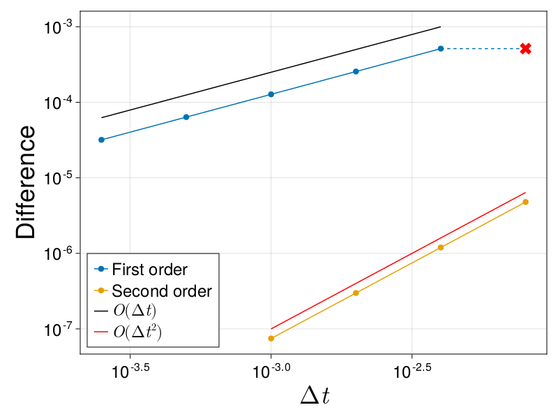
Figure 1: Convergence plot demonstrating first and second-order accuracy in time of the respective time integrators. The first-order integrator is unstable for $\Delta t=$8\text{\times}{10}^{-3}$$.

6.2 Weak Landau damping

As a physics test, we reproduce the ubiquitous weak Landau damping benchmark problem with wavenumber $k=0.5$ using both the Hermite spectral discretization and the Legendre-weighted finite difference discretization in velocity.

The initial condition is

$$f_{0}(x,v)=(1+\delta\cos(kx))e^{-v^{2}/2},\quad x\in(0,2\pi/k).$$

The perturbation size is set to $\delta=$1\text{\times}{10}^{-3}$$. The domain is discretized with $N_{x}=128$ points in the $x$ direction and with either $M=256$ Hermite modes or $N_{v}=256$ velocity grid points. The rank is set to $r=6$. We run the simulation with the second-order integrator to time $t=40$, using timesteps of $\Delta t=$2\text{\times}{10}^{-3}$$. The result is shown in Figure 2. We measure a damping rate of $\gamma=-0.1525$ for the Hermite spectral discretization and $\gamma=-0.1523$ for the finite difference discretization of velocity space, demonstrating good agreement with the linear theory prediction of $\gamma=-0.153$.

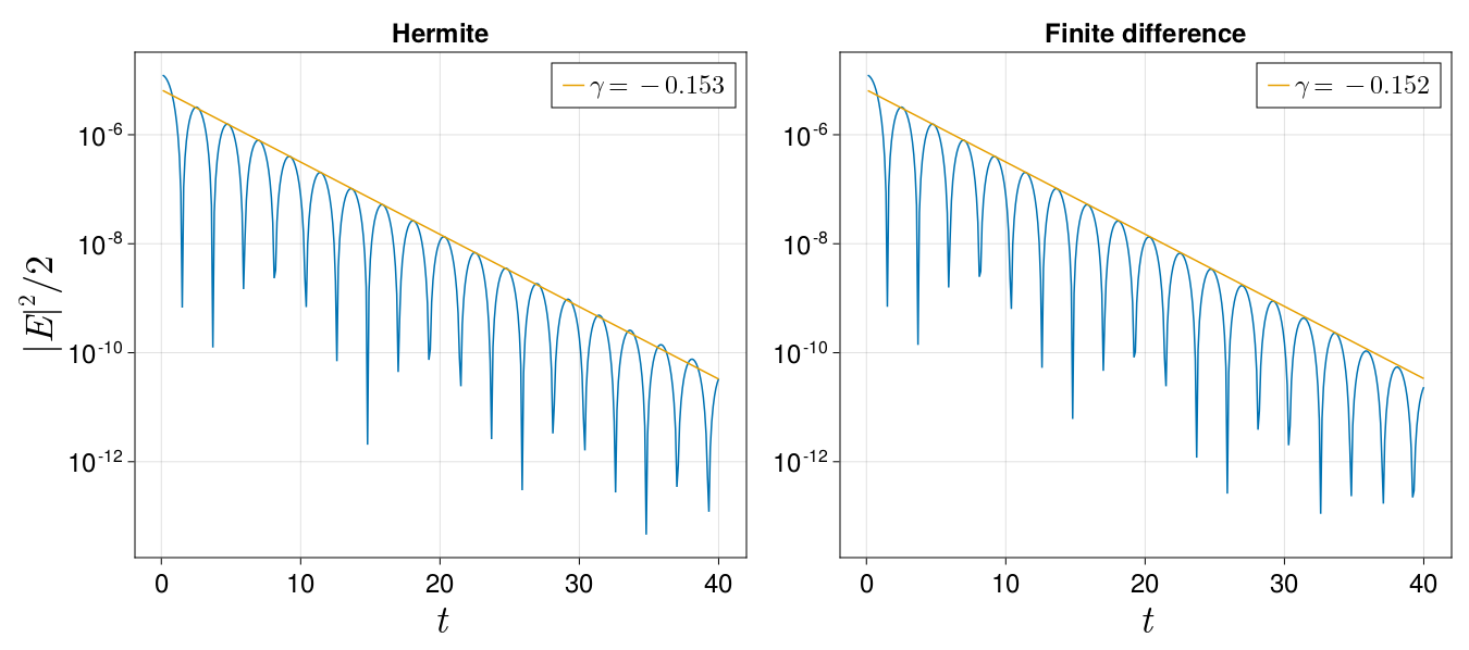
(a) Electric energy and best linear fit.

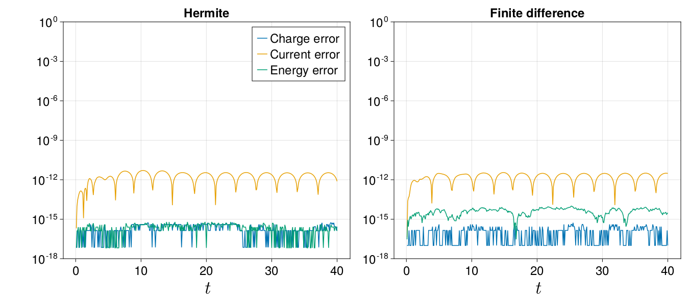
(b) Charge, current and energy conservation error.

Figure 2: Weak Landau damping example, demonstrating exact conservation of charge and energy with the second-order time integrator.

Collisional Landau damping

We validate the correctness of our solver including collisionality by comparing the Landau damping phenomenon at a variety of collision frequencies $\nu$. We solve the same weak Landau damping problem as above, but with the collision frequency $\nu$ set to $0.0,0.25,$ and $1.0$. The Hermite spectral solver is run with $M=256$ and $\Delta t=$2\text{\times}{10}^{-3}$$, the same as the collisionless example. In contrast, the finite difference velocity discretization becomes more stiff as the diffusive collision term grows larger, so for that discretization we reduce both the velocity grid spacing and timestep to $N_{v}=128$ grid points and $\Delta t=$5\text{\times}{10}^{4}$$. The results are shown in Figure 3.

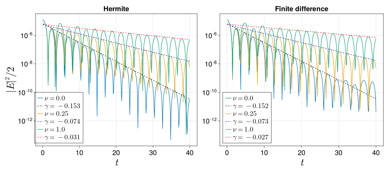
(a) Measured damping rates as a function of collision frequency $\nu$. Increasing collisionality brings the solution nearer to the fluid limit, which experiences no damping. Our results agree well with published results in [23].

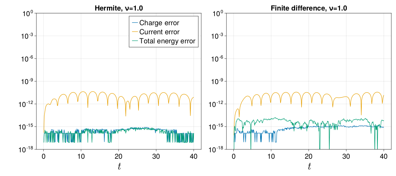
(b) Conservation of charge and energy by the second-order integrator, tested in the $\nu=1.0$ case.

Figure 3: Collisional Landau damping example.

6.3 Strong Landau damping

In this example we use the same wavenumber and domain as the weak Landau damping problem, $k=0.5$, but set $\delta=0.5$ to explore the strong (nonlinear) Landau damping regime. Again we present results from both the Hermite spectral and finite difference discretizations in velocity space. The simulation is run with $r=16$, on a grid with $N_{x}=128$ grid points in $x$, and either $M=256$ Hermite modes or $N_{v}=256$ velocity grid points. The timestep is set to $\Delta t=$4\text{\times}{10}^{-3}$$, and the initial condition is evolved using the second-order energy-conserving integrator to $t=50.0$. The results are shown in Figure 4, including the phase space density at $t=25.0$. Conservation properties of both first and second order integrators on this strong Landau damping problem are shown in Figure 5.

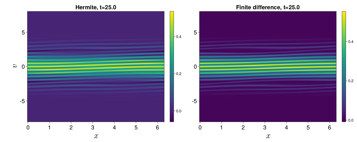
(a) Phase space distribution $f(x,v,t=25.0)$ showing strong filamentation.

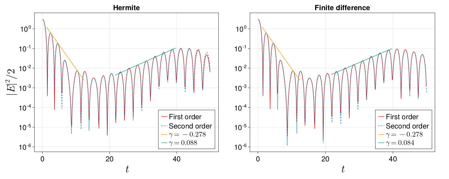
(b) Electric energy traces. Our implementation matches both the initial nonlinear damping and subsequent growth rates, compared to published results such as [24].

Figure 4: Strong Landau damping example.

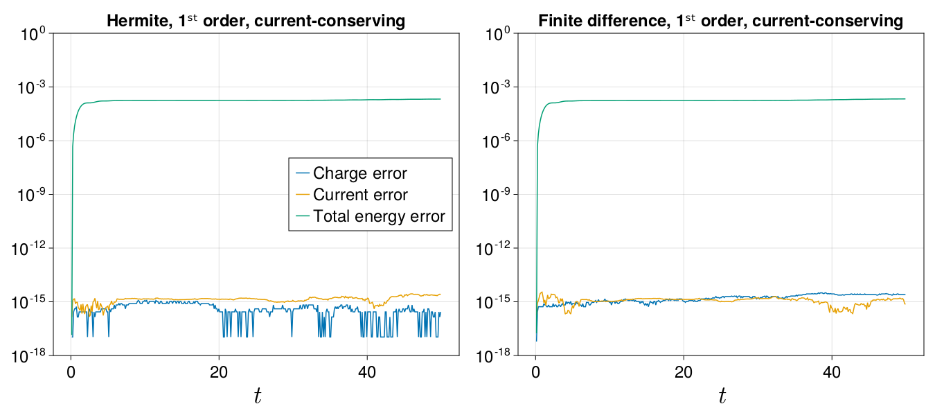
(a) Exact conservation of charge and current by the first order integrator with a Poisson solve.

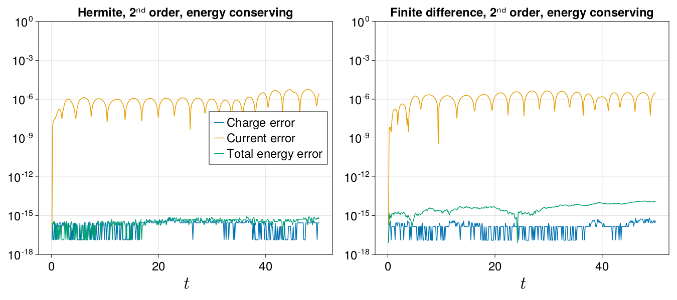
(b) Exact conservation of charge and energy by the second order integrator with an Ampère solve.

Figure 5: Conservation plots in the strong Landau damping example. We observe the benefit of overall second-order accuracy in the improved conservation of current in (b), compared to the conservation error of energy in (a).

6.4 Two-stream instability

Here we reproduce the two-stream instability example from [15]:

$$f(x,v,0)=\frac{2}{7}(1+5v^{2})(1+\delta((\cos(2kx)+\cos(3kx))/1.2+\cos(kx)))\frac{1}{\sqrt{2\pi}}e^{-v^{2}/2},$$

with $\delta=0.01,k=0.5$. This form of the distribution function is chosen to give the following analytic forms for the zeroth and second Hermite moments:

$$f_{0}^{\text{Hermite}}(x,0)=\frac{12}{7}(1+\delta((\cos(2kx)+\cos(3kx))/1.2+\cos(kx))),$$

$$f_{2}^{\text{Hermite}}(x,0)=\frac{10\sqrt{2}}{7}(1+\delta((\cos(2kx)+\cos(3kx))/1.2+\cos(kx))).$$

We run this simulation on a grid with $N_{x}=256$ grid points in $x$. For the Hermite spectral discretization we use $M=256$ Hermite modes, and for the finite difference discretization we use $N_{v}=256$ velocity grid points. The rank is set to $r=20$, and the instability is evolved with $\Delta t=$4\text{\times}{10}^{-3}$$ well into the nonlinear phase, up to $t=50.0$. The results are shown in Figure 6.

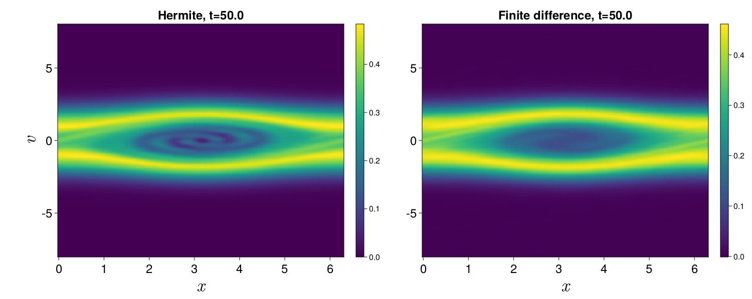
(a) Plots of $f(x,v,t=50.0)$, depicting nonlinear phase space trapping in the two-stream instability.

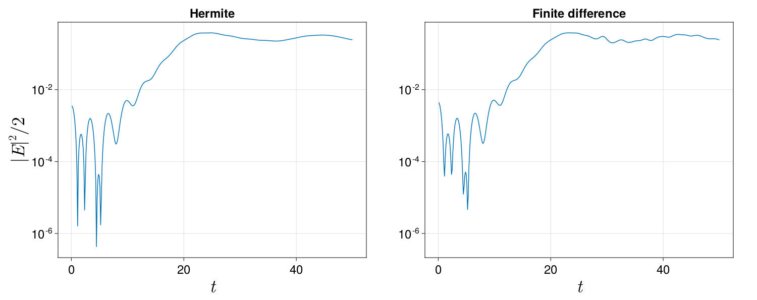
(b) Electric energy trace. Our results show excellent agreement with published numerical results in [15].

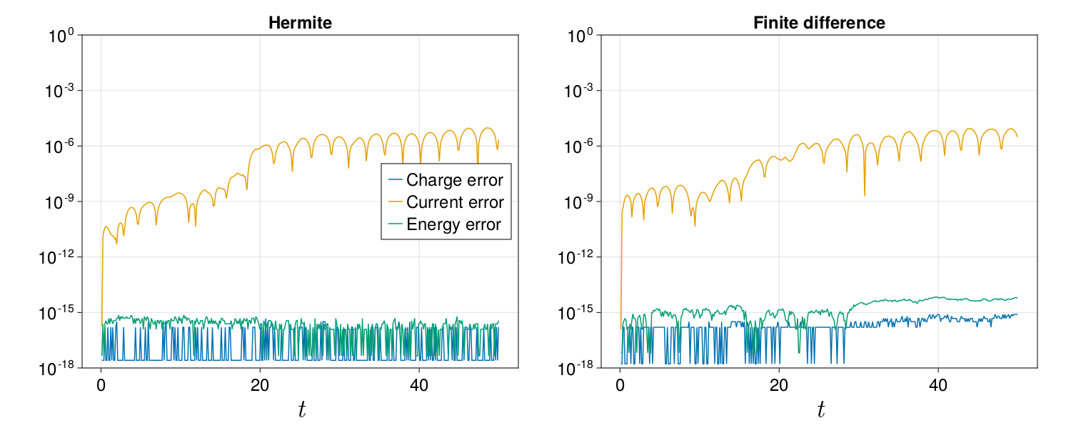
(c) Exact conservation of charge and energy by the second order integrator.

Figure 6: Two-stream instability.

7 Conclusion

We have demonstrated a novel macro-micro decomposition which separates the particle distribution function $f$ into a rank-3 macroscopic portion which shares the moments of $f$, and a microscopic part which may be evolved in the dynamical low-rank approximation framework. This separation leads to a method which shares the efficiency benefits of the standard DLR approach while preserving conservation of charge, current, and kinetic energy density. Our macro-micro decomposition can be combined with appropriate temporal and spatial discretizations to obtain schemes which exactly conserve charge and either current or energy, and achieve second-order accuracy in time.

To construct the decomposition, we use the orthogonal polynomial family corresponding to a weighted inner product over velocity space to form an orthogonal projection which effectively separates the macroscopic and microscopic portions of $f$. Our approach has the benefit of supporting both infinite and truncated velocity domains. Because the decomposition happens at the equation level, one can choose any discretization of velocity space which is suitable for the application at hand. To demonstrate this flexibility, we have implemented both a Hermite global spectral discretization and a conservative finite difference discretization of velocity space.

As a proof of concept, we have implemented this scheme in one dimension, demonstrating the effectiveness of the approach on standard plasma test problems. We anticipate that extending the scheme to multiple dimensions should pose no essential difficulty, since one can obtain a similar macro-micro decomposition based on tensor products of orthgonal polynomials. Similarly, applying our scheme to the full Vlasov-Maxwell system would capture fully electromagnetic physics without disproportionate complications.

References

- [1] ıt NIST Digital Library of Mathematical Functions.
- [2] Mounir Bennoune, Mohammed Lemou, and Luc Mieussens. Uniformly stable numerical schemes for the Boltzmann equation preserving the compressible Navier–Stokes asymptotics. Journal of Computational Physics, 227(8):3781–3803, April 2008.
- [3] Charles K. Birdsall and A. Bruce Langdon. Plasma physics via computer simulation. McGraw-Hill, New York, 1985.
- [4] Gianluca Ceruti and Christian Lubich. An unconventional robust integrator for dynamical low-rank approximation. BIT Numerical Mathematics, 62(1):23–44, March 2022.
- [5] Jack Coughlin and Jingwei Hu. Efficient dynamical low-rank approximation for the Vlasov-Ampère-Fokker-Planck system. Journal of Computational Physics, page 111590, September 2022.
- [6] G.L. Delzanno. Multi-dimensional, fully-implicit, spectral method for the Vlasov–Maxwell equations with exact conservation laws in discrete form. Journal of Computational Physics, 301:338–356, November 2015.
- [7] J. P. Dougherty. Model Fokker-Planck Equation for a Plasma and Its Solution. Physics of Fluids, 7(11):1788, 1964.
- [8] Lukas Einkemmer. Accelerating the simulation of kinetic shear Alfvén waves with a dynamical low-rank approximation. 2023. Publisher: arXiv Version Number: 1.
- [9] Lukas Einkemmer, Jingwei Hu, and Yubo Wang. An asymptotic-preserving dynamical low-rank method for the multi-scale multi-dimensional linear transport equation. Journal of Computational Physics, 439:110353, August 2021.
- [10] Lukas Einkemmer, Jingwei Hu, and Lexing Ying. An Efficient Dynamical Low-Rank Algorithm for the Boltzmann-BGK Equation Close to the Compressible Viscous Flow Regime. SIAM Journal on Scientific Computing, 43(5):B1057–B1080, January 2021.
- [11] Lukas Einkemmer and Ilon Joseph. A mass, momentum, and energy conservative dynamical low-rank scheme for the Vlasov equation. Journal of Computational Physics, 443:110495, October 2021.
- [12] Lukas Einkemmer and Christian Lubich. A Low-Rank Projector-Splitting Integrator for the Vlasov–Poisson Equation. SIAM Journal on Scientific Computing, 40(5):B1330–B1360, January 2018.
- [13] Lukas Einkemmer and Christian Lubich. A Quasi-Conservative Dynamical Low-Rank Algorithm for the Vlasov Equation. SIAM Journal on Scientific Computing, 41(5):B1061–B1081, January 2019.
- [14] Lukas Einkemmer, Alexander Ostermann, and Carmela Scalone. A robust and conservative dynamical low-rank algorithm. Journal of Computational Physics, 484:112060, July 2023.
- [15] Francis Filbet and Tao Xiong. Conservative Discontinuous Galerkin/Hermite Spectral Method for the Vlasov–Poisson System. Communications on Applied Mathematics and Computation, 4(1):34–59, March 2022.
- [16] Walter Gautschi. Orthogonal Polynomials: Computation and Approximation. Oxford University Press, April 2004.
- [17] Sigal Gottlieb, David Ketcheson, and Chi-Wang Shu. Strong Stability Preserving Runge-Kutta and Multistep Time Discretizations. WORLD SCIENTIFIC, January 2011.
- [18] Harold Grad. On the kinetic theory of rarefied gases. Communications on Pure and Applied Mathematics, 2(4):331–407, December 1949.
- [19] Wei Guo, Jannatul Ferdous Ema, and Jing-Mei Qiu. A Local Macroscopic Conservative (LoMaC) Low Rank Tensor Method with the Discontinuous Galerkin Method for the Vlasov Dynamics. Communications on Applied Mathematics and Computation, July 2023.
- [20] Wei Guo and Jing-Mei Qiu. A conservative low rank tensor method for the Vlasov dynamics. arXiv:2201.10397 [cs, math], January 2022. arXiv: 2201.10397.
- [21] Wei Guo and Jing-Mei Qiu. A Local Macroscopic Conservative (LoMaC) low rank tensor method for the Vlasov dynamics, July 2022. arXiv:2207.00518 [cs, math].
- [22] Wei Guo and Jing-Mei Qiu. A Low Rank Tensor Representation of Linear Transport and Nonlinear Vlasov Solutions and Their Associated Flow Maps. Journal of Computational Physics, 458:111089, June 2022. arXiv:2106.08834 [cs, math].
- [23] Ammar Hakim, James Juno, and Gregory W. Hammett. Conservative discontinuous Galerkin schemes for nonlinear Dougherty–Fokker–Planck collision operators. Journal of Plasma Physics, 86(4):905860403, August 2020.
- [24] Andrew Ho, Iman Anwar Michael Datta, and Uri Shumlak. Physics-Based-Adaptive Plasma Model for High-Fidelity Numerical Simulations. Frontiers in Physics, 6:105, September 2018.
- [25] Thomas Y. Hou and Ruo Li. Computing nearly singular solutions using pseudo-spectral methods. Journal of Computational Physics, 226(1):379–397, September 2007.
- [26] Jingwei Hu and Yubo Wang. An Adaptive Dynamical Low Rank Method for the Nonlinear Boltzmann Equation. Journal of Scientific Computing, 92(2):75, August 2022.
- [27] Othmar Koch and Christian Lubich. Dynamical Low‐Rank Approximation. SIAM Journal on Matrix Analysis and Applications, 29(2):434–454, January 2007.
- [28] O. Koshkarov, G. Manzini, G.L. Delzanno, C. Pagliantini, and V. Roytershteyn. The multi-dimensional Hermite-discontinuous Galerkin method for the Vlasov–Maxwell equations. Computer Physics Communications, 264:107866, July 2021.
- [29] Christian Lubich and Ivan V. Oseledets. A projector-splitting integrator for dynamical low-rank approximation. BIT Numerical Mathematics, 54(1):171–188, March 2014.
- [30] C.-D. Munz, P. Ommes, and R. Schneider. A three-dimensional finite-volume solver for the Maxwell equations with divergence cleaning on unstructured meshes. Computer Physics Communications, 130(1-2):83–117, July 2000.
- [31] Zhuogang Peng and Ryan G. McClarren. A high-order/low-order (HOLO) algorithm for preserving conservation in time-dependent low-rank transport calculations. Journal of Computational Physics, 447:110672, December 2021.
- [32] Zhuogang Peng, Ryan G. McClarren, and Martin Frank. A low-rank method for two-dimensional time-dependent radiation transport calculations. Journal of Computational Physics, 421:109735, November 2020.
- [33] Chi-Wang Shu. Essentially non-oscillatory and weighted essentially non-oscillatory schemes for hyperbolic conservation laws. In Alfio Quarteroni, editor, Advanced Numerical Approximation of Nonlinear Hyperbolic Equations, volume 1697, pages 325–432. Springer Berlin Heidelberg, Berlin, Heidelberg, 1998. Series Title: Lecture Notes in Mathematics.
- [34] Chi-Wang Shu. High Order Weighted Essentially Nonoscillatory Schemes for Convection Dominated Problems. SIAM Review, 51(1):82–126, February 2009.
- [35] Juris Vencels, Gian Luca Delzanno, Gianmarco Manzini, Stefano Markidis, Ivy Bo Peng, and Vadim Roytershteyn. SpectralPlasmaSolver: a Spectral Code for Multiscale Simulations of Collisionless, Magnetized Plasmas. Journal of Physics: Conference Series, 719:012022, May 2016.