HypOp: Distributed Constrained Combinatorial Optimization leveraging Hypergraph Neural Networks

Abstract

Scalable addressing of high dimensional constrained combinatorial optimization problems is a challenge that arises in several science and engineering disciplines. Recent work introduced novel application of graph neural networks for solving polynomial-cost unconstrained combinatorial optimization problems. This paper proposes a new framework, called HypOp, which greatly advances the state of the art for solving combinatorial optimization problems in several aspects: (i) it generalizes the prior results to constrained optimization problems with an arbitrary cost function; (ii) it broadens the application to higher dimensional problems by leveraging a hypergraph neural network structure; (iii) it enables scalability to much larger problems by introducing a new distributed and parallel architecture for hypergraph neural network training; (iv) it demonstrates generalizability to other problem formulations by knowledge transfer from the learned experience of addressing one set of cost/constraints to another set for the same hypergraph; (v) it significantly boosts the solution accuracy compared with the prior art by suggesting a fine-tuning step using simulated annealing; (vi) HypOp shows a remarkable progress on benchmark examples, with run times improved by up to fivefold using a combination of fine-tuning and distributed training techniques. The framework allows addressing a novel set of scientific problems including hypergraph MaxCut problem, satisfiability problems (3SAT), and resource allocation. We showcase the application of HypOp in scientific discovery by solving a hypergraph MaxCut problem on the NDC drug-substance hypergraph. Through extensive experimentation on a variety of combinatorial optimization problems, HypOp demonstrates superiority over existing unsupervised learning-based solvers and generic optimization methods.

I Introduction

Combinatorial optimization is ubiquitous across science and industry. Scientists often need to make decisions about how to allocate resources, design experiments, schedule tasks, or select the most efficient pathways among numerous choices. Combinatorial optimization techniques can help in these situations by finding the optimal or near-optimal solutions, thus aiding in the decision-making process. Furthermore, the integration of artificial intelligence (AI) into the field of scientific discovery is growing increasingly fluid, providing a means to enhance and accelerate research [39]. An approach to integrate AI into scientific discovery involves leveraging machine learning (ML) methods to expedite and improve the combinatorial optimization techniques to solve extremely challenging optimization tasks. Several combinatorial optimization problems are proved to be NP-hard, rendering most existing solvers non-scalable. The continually expanding size of today’s datasets makes existing optimization methods inadequate for addressing constrained optimization problems across such vast datasets. To facilitate the development of scalable and rapid optimization algorithms, various learning-based approaches have been proposed in the literature [36, 8].

Learning-based optimization methods can be classified into three main categories: supervised learning, unsupervised learning, and reinforcement learning (RL)-based approaches. Supervised methods [20, 4, 14, 33, 27] train a model to address the given problems using a dataset of solved problem instances. However, these approaches exhibit limitations in terms of generalizability to problem types not present in the training dataset and tend to perform poorly when handling larger problem sizes. Unsupervised learning-based approaches [36, 19, 38] do not rely on datasets of solved instances. Instead, they train ML models using optimization objectives as their loss functions. Unsupervised methods offer several advantages over supervised ones, including enhanced generalizability and eliminating the need for datasets containing solved problem instances, which can be challenging to acquire. RL-based methods [31, 44, 29, 24] hold promise for specific optimization problems, provided that lengthy training and fine-tuning times can be accommodated.

Unsupervised learning based optimization methods can be conceptualized as a fusion of gradient descent-based optimization techniques with learnable transformation functions. In particular, in an unsupervised learning-based optimization algorithm, the original optimization variables are generated through an ML model, and the objective function is optimized by applying gradient descent over the parameters of this model. In other words, instead of conducting gradient descent directly on the optimization variables, it is applied to the parameters of the function (the ML model) responsible for generating those optimization variables. The goal is to establish a more efficient optimization path compared to conventional direct gradient descent. This approach can potentially facilitate more effective escapes from subpar local optima. Various transformation functions are utilized in the optimization literature to convert the problem into a more tractable form. For example, there are numerous techniques to linearize or convexify an optimization problem by employing transformation functions that are often lossy [3]. We believe that adopting ML-based transformation functions for optimization offers a significant capability to train a customized transformation function that best suits the specific optimization task.

For combinatorial optimization problems over graphs, graph neural networks are frequently employed as the learnable transformation functions [36, 19, 38]. However, when dealing with more complex systems with higher order interactions and constraints, graphs fall short of modeling such relations. When intricate relationships among multiple entities extend beyond basic pairwise connections, hypergraphs emerge as invaluable tools for representing a diverse array of scientific phenomena. They have been utilized in various areas including biology and bioinformatics [12, 32], social network analysis [45], chemical and material science [42], image and data processing [40]. Hypergraph neural networks (HyperGNN) [13] have also been commonly used for certain learning tasks such as image and visual object classification [13], and material removal rate prediction [42]. It is anticipated that hypergraph neural networks may serve as the suitable learnable transformation functions for solving combinatorial optimization problems with higher-order constraints.

While unsupervised learning-based approaches for solving combinatorial optimization problems offer several advantages, they may encounter limitations such as susceptibility of getting trapped in suboptimal local solutions and scaling effectively to larger problem instances. In a recent work [2], the authors argue that for certain well-known combinatorial optimization problems, unsupervised learning-based optimization methods may exhibit inferior performance compared to straightforward heuristics. However, it is crucial to recognize that these unsupervised methods possess a significant advantage in their generic applicability. Generic solvers like gradient-based techniques (such as SGD and ADAM), as well as simulated annealing (SA), may not be able to compete with customized heuristics that are meticulously crafted for specific problems. Nonetheless, they serve as invaluable tools for addressing less-known problems lacking effective heuristics. Consequently, the strategic utilization of unsupervised learning-based optimization methods can enhance and extend the capabilities of existing generic solvers, leading to the development of more efficient tools for addressing a diverse range of optimization problems.

In this study, we build upon the unsupervised learning-based optimization method for polynomial-cost combinatorial optimization problems on graphs introduced in [36], and present HypOp, a new scalable solver for a wide range of constrained combinatorial optimization problems with arbitrary cost functions. Our approach is applicable to problems with higher-order constraints by adopting hypergraph modeling for such problems (Fig. 1(a)); HypOp subsequently utilizes hypergraph neural networks in the training process, a generalization of the graph neural networks employed in [36]. HypOp further proposes combining unsupervised hypergraph neural networks with other generic optimization methods including simulated annealing [23] and black-box sampling based optimizers [18]. Incorporating SA with HyperGNN can help with mitigation of the potential subpar local optima that may arise from HyperGNN training.

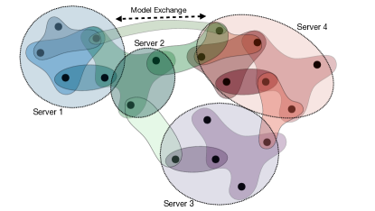
To establish a scalable solver and expedite the optimization process, HypOp proposes two algorithms for parallel and distributed training of HyperGNN. First, it develops a distributed training algorithm in which, the hypergraph is partitioned between a number of servers and each server only has a local view of the hypergraph. We develop a collaborative distributed algorithm to train the HyperGNN and solve the optimization problem (See Fig. 1(b)). Second, HypOp proposes a parallel HyperGNN training approach where the costs associated to constraints are computed in a scalable manner. We further exhibit the transferability of our models, highlighting their efficacy in solving different optimization problems on the same hypergraph through transfer learning. This not only shows the generalizability of HypOp but also significantly accelerates the optimization process. HypOp is tested by comprehensive experiments, thoughtfully designed to provide insights into unsupervised learning-based optimization algorithms and their efficacy across diverse problem types. We validate the scalability of HypOp by testing it on huge graphs, showcasing how parallel and distributed training can yield high-quality solutions even on such massive graphs. In summary, our contributions are as follows.

(a) Hypergraph Modeling of the Constraint Combinatorial Optimization Problem in HypOp.

(b) Distributed HyperGNN training in HypOp.

Figure 1: Hypergraph modeling and Distributed Training of HyperGNN in HypOp

• Presenting HypOp, a scalable unsupervised learning-based optimization method for addressing a wide spectrum of constrained combinatorial optimization problems with arbitrary cost functions. Notably, we pioneer the application of hypergraph neural networks within the realm of learning-based optimization for general combinatorial optimization problems with higher order constraints.

• Enabling scalability to much larger problems by introducing a new distributed and parallel architecture for hypergraph neural network training.

• Demonstrating generalizability to other problem formulations, by knowledge transfer from the learned experience of addressing one set of cost/constraints to another set for the same hypergraph.

• Significantly boosting the solution accuracy and improving run times by up to fivefold using a combination of fine-tuning (simulated annealing) and distributed training techniques.

• Demonstrating superiority of HypOp over existing unsupervised learning-based solvers and generic optimization methods through extensive experimentation on a variety of combinatorial optimization problems. We address a novel set of scientific problems including hypergraph MaxCut problem, satisfiability problems (3SAT), and resource allocation.

• Showcasing the application of HypOp in scientific discovery by solving a hypergraph MaxCut problem on the NDC drug-substance hypergraph.

I-A Related Work

The recent significant progress in the ML has prompted its application in optimization [5, 9, 28, 15]. Combinatorial optimization, given its intricate nature, stands to benefit greatly from learning-based approaches [5, 26, 8, 31, 36]. Learning methods for combinatorial optimization problems can be categorized into supervised learning [20, 4, 14, 33, 27], unsupervised learning [36, 19, 38], and reinforcement learning [31, 44, 29, 24]. Although supervised learning methods have shown promising results in various combinatorial optimization problems, they need a dataset of solved instances, posing challenges of computational intensity, expense, and limited generalizability to new or larger problems. Reinforcement learning is a powerful tool for optimization and has been proved to be effective for many problems. However, training RL models is usually challenging and time-consuming. Therefore, RL methods are best to be used for finding efficient algorithms to solve specific problems [11]. Unsupervised learning methods enable fast and generalizable optimization of combinatorial optimization problems without requiring a dataset of solved problem instances. One issue with unsupervised learning methods is that they are based on gradient descent and therefore, they may converge to subpar local optima.

To address the issues of the unsupervised learning methods getting stuck at local optima, [37] proposed an annealed training framework for combinatorial optimization problems over graphs. A smoothing term is added to the loss function to help the training process escape the local optima. This smoothing strategy can be combined with any unsupervised learning method for combinatorial optimization including the method described in this paper.

While there is no existing research that models constrained combinatorial optimization problems as hypergraphs to capture higher-level dependencies between variables, a study has approached maximum constraint satisfiability problems by modeling them as bipartite graphs and training a Graph Neural Network (GNN) to find solutions [38]. However, it is limited to problems with constraints involving only two variables and is not suitable for problems with different types of constraints, such as 3-SAT.

I-B Paper Structure

The remainder of this paper is structured as follows. We describe the notations used throughout the paper in Section II. Some preliminary concepts are explained in Section III. We have the problem statement in Section IV. The HypOp method is presented in Section V. We describe two algorithms for distributed and scalable training of HypOp in Section VI. Our experimental results are provided in Section VII. We showcase the possibility of transfer learning in HypOp in Section VIII. The applications of HypOp in scientific discovery is discussed in Section IX. The limitations of the unsupervised learning-based methods are presented in Section X. We conclude by a discussion in Section XI.

II Notations

We use lower case letters to show scalars, vectors and functions. Matrices are denoted by upper case letters. For a set of scalars $x_{i},\ i=1,\cdots,N$, we drop the index to show the vector of those scalars, i.e., $x=[x_{1},\cdots,x_{N}]$. For a matrix $X$, $diag(X)$ is defined as the diagonal matrix consisting of the diagonal entries of matrix $X$.

III Preliminaries: Graph and Hypergraph Neural Networks

III-A Graph Neural Networks

Graph neural network (GNN) [41] is a type of ML model that is designed for analyzing data structured as graphs. GNN have shown to be able to capture intricate patterns and dependencies within graph-structured data, making them useful for tasks such as node classification, link prediction, and graph-level analysis. GNNs operate by iteratively aggregating information from a node’s neighbors and using this information to update the node’s own features. Graph convolutional networks (GCN) [22] are a specific types of GNNs and the layer-wise operation can be described as below:

$$H^{(l+1)}=\sigma(\tilde{D}^{-\frac{1}{2}}\tilde{A}^{-1}\tilde{D}^{-\frac{1}{2}}H^{(l)}W^{(l)})$$ (1)

where $H^{(l)}\in\mathbb{R}^{N\times D}$ is the matrix of node features at $l_{th}$ layer, $\tilde{A}$ is the adjacency matrix of the graph with added self loops, $\tilde{D}$ is the diagonal degree matrix of $\tilde{A}$, and $W^{(l)}$ is the $l_{th}$ layer trainable weight matrix.

III-B Hypergraph Neural Network

A hypergraph is a generalized version of a graph in which, instead of having edges connecting two nodes, we have hyperedges connecting multiple nodes to each other, allowing for more complex relationships than traditional graphs. Hypergraph neural network (HyperGNN) [13] is an advanced variation of graph neural networks that is designed to handle hypergraphs. HyperGNNs extend the concept of GNNs to hypergraphs by introducing new aggregation mechanisms that consider higher-order connections (hyperedges). HyperGNNs can capture intricate dependencies among multiple nodes simultaneously, making them well-suited for tasks involving data with complex associations, such as social interactions, collaboration data, knowledge graphs, and recommendation systems. In hypergraph convolutional networks introduced in [13], features of nodes are first aggregated in each hyperedge and are then passed on to new nodes for another aggregation. In particular, we have the following layer-wise operation:

$$H^{(l+1)}=\sigma(D_{v}^{-\frac{1}{2}}{A}D_{e}^{-1}A^{T}D_{v}^{-\frac{1}{2}}H^{(l)}W^{(l)})$$ (2)

where $H^{(l)}\in\mathbb{R}^{N\times D}$ is the matrix of node features at $l_{th}$ layer, $A$ is the hypergraph incidence matrix defined as $(A)_{ij}=1$ if node $i$ belongs to hyperedge $j$, and $(A)_{ij}=0$ otherwise. $D_{v}$ and $D_{e}$ are the diagonal degree matrices of nodes and hyperedges, respectively, and $W^{(l)}$ is the $l_{th}$ layer trainable weight matrix.

IV Problem Statement

We consider a constrained combinatorial optimization problem over $x_{i},\ i\in\mathcal{N}$, where $\mathcal{N}=\{1,\cdots,N\}$ is the set of optimization variable indices. The variables $x_{i}$ are integers belonging to the set $\{d_{0},\cdots,d_{v}\}$, where $d_{0},\cdots,d_{v}$ are some given integers and $d_{i}<d_{j}$ for $i<j$ (We can also have a combination of real and integer variables). There are $K$ constraint functions, $c_{k}(x_{\mathcal{N}_{k}}),\ k\in\mathcal{K}$, where $\mathcal{K}=\{1,\cdots,K\}$ is the set of constraint indices, and $x_{\mathcal{N}_{k}}=\{x_{i},i\in\mathcal{N}_{k}\}$, and we have $\mathcal{N}_{k}\subset\mathcal{N}$. The cost function of the optimization is denoted as $f(x)$. The optimization problem that we consider is given below.

$$\min_{x_{i},i\in\mathcal{N}}\quad f(x)$$ (3a)

$$s.t.\quad c_{k}(x_{\mathcal{N}_{k}})\leq 0,\ \text{for}\ k\in\mathcal{K}$$ (3b)

$$x_{i}\in\{d_{0},\cdots,d_{v}\},\ \text{for}\ i\in\mathcal{N}$$ (3c)

Since the above optimization problem is over discrete variables, and the objective and constraint functions are potentially non-linear and non-convex, this problem is usually NP-hard and efficiently solving it is a complex task. On the other hand, the discreteness of the optimization variables indicates that the objective function is not a continuous function and consequently, gradient descent-based approaches may not be used. One common approach for solving such problems over discrete variables is to relax the state space into continuous spaces and solve the relaxed problem, now with a continuous objective function. Consequently, gradient descent-based methods can be used to solve the problem. A mapping between continuous to discrete values is required once the optimized continuous values are obtained. We note that the obtained solutions are not guaranteed to be globally optimal due to two reasons. First, the problem is solved in its relaxed format and not its original format. Second, the gradient descent solver can converge a subpar local optima. However, these approaches are still one of the most common practices to solve such problems due to the availability and efficiency of the gradient descent-based solvers. These solvers such as ADAM [21] are widely developed and used as the main optimization method for ML tasks.

In order to relax the optimization problem (3), we define $p_{i}$ to be the continuous (relaxed) version of $x_{i}$, and allow the variables $p_{i}$ to belong to the continuous range of $[d_{0}-d_{v}]$. The relaxed version of the optimization problem in (3) is given below.

$$\min_{p_{i},i\in\mathcal{N}}\quad f(p)$$ (4a)

$$s.t.\quad c_{k}(p_{\mathcal{N}_{k}})\leq 0,\ \text{for}\ k\in\mathcal{K}$$ (4b)

$$p_{i}\in[d_{0}-d_{v}],\ \text{for}\ i\in\mathcal{N}$$ (4c)

V HypOp Method

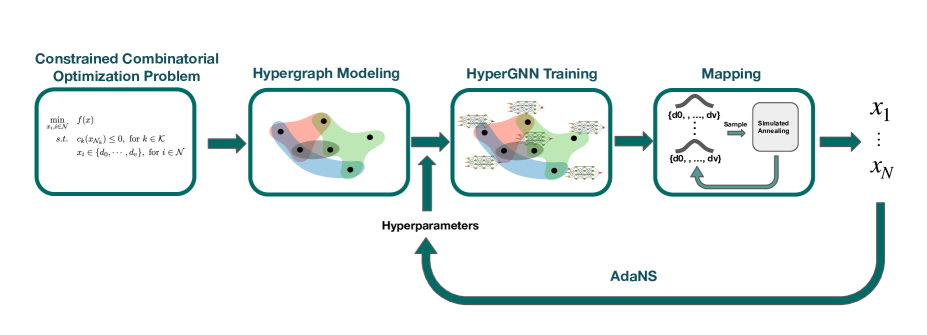
In this section, we describe our method for solving problem (3). Fig. 2 is an overview of our algorithm, where each part will be explained later. We refer to our algorithm as HypOp. The main steps of the algorithms are: (1) hypergraph modeling of the problem, (2) solving the relaxed version of the optimization problem (problem (4)) using hypergraph neural networks in an unsupervised learning manner, and (3) mapping the continuous variable (node) values to discrete ones using a post-processing mapping algorithm. (4) We have also considered the optional step of optimizing over the hyperparameters of the algorithm using a sampling-based black-box optimization tool.

Figure 2: The overview of HypOp for solving problem (3).

In the following, we describe each step of HypOp in more details.

V-A Hypergraph Modeling

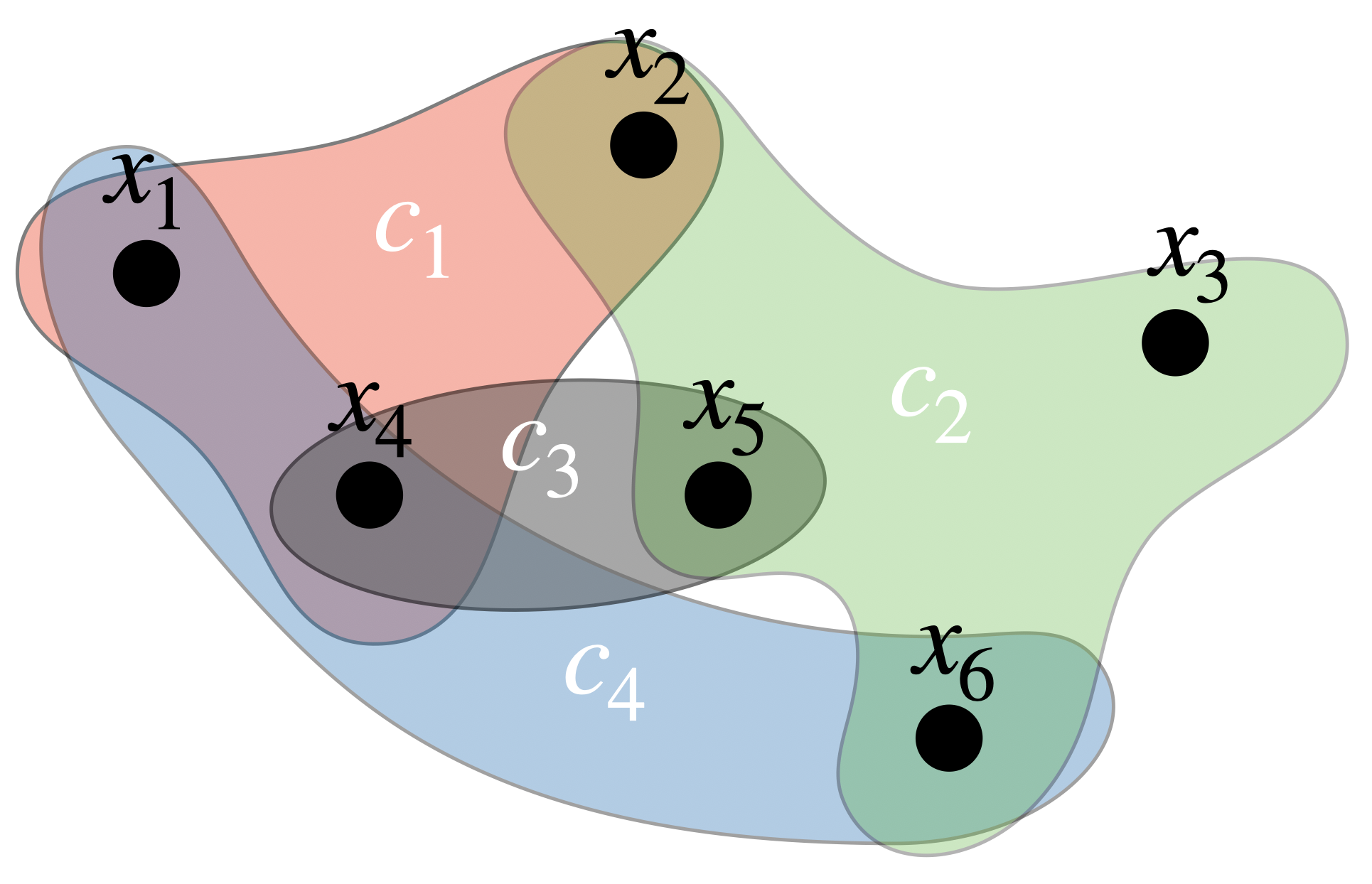
In order to utilize hypergraph neural networks to solve problem (3) (or (4)), we model the constraints of this problem by a hypergraph as follows. Consider a hypergraph with nodes $x_{i},\ i\in\mathcal{N}$. For each constraint $c_{k}(x_{\mathcal{N}_{k}})$, we put a hyperedge consisting of nodes $x_{\mathcal{N}_{k}}$. We refer to this hypergraph as the constraint hypergraph of the problem. For example, for a problem with 6 variables and 4 constraints, the constraint hypergraph is given in Fig. 1(a).

We note that solving problem (3) is equivalent with a node classification over the constraint hypergraph where the assigned classes of the nodes satisfy constraints corresponding to their hyperedges and are minimizing the cost function. Note that for the problems with an underlying graph or hypergraph structure, such as graph MaxCut, the constraint hypergraph will be the underlying graph or hypergraph of the problem.

V-B HyperGNN as the Learnable Transformation Function

One can solve optimization problem (4) directly using gradient descent-based methods and then map the continuous outcomes to the discrete values. Penalty-based method are a common practice in these approaches to ensure the constraints are satisfied in the final outcome. However, as we will show in this paper, solving an alternative optimization problem, in which the optimization variables $p_{i}$ are the outcome of a HyperGNN-based transformation function, will result in better solutions. Various transformation functions are utilized in the optimization literature to transform an optimization problem into a form that is more tractable. For example, there are numerous techniques to linearize an optimization problem with the use of transformation functions [3]. However, in most of the existing literature, the transformation function is a fixed function. In HypOp, we consider a parameterized transformation function that is based on HyperGNNs. In particular, we consider $p=\mathcal{G}(\sigma;W)$, where $W$ is the parameter vector of the transformation function, $\mathcal{G}$, and $\sigma=[\sigma_{1},\cdots,\sigma_{N}]$ is the input embedding. We also use the notation $p_{i}=\mathcal{G}_{i}(\sigma;W)$, where $p_{i}$ is the (continuous) assignment to node $i$ by the HyperGNN. By considering a parameterized transformation function, we optimize our objective by learning a good transformation function (learn $W$) at the same time as optimizing the input embedding ($\sigma$).

Defining the constraint hypergraph of the optimization problem (4) enables us to use hypergraph neural networks to model our transformation function, $\mathcal{G}(\sigma;W)$, where $\sigma_{i}$ is the input feature of node $i$ of the hypergraph neural network and $W$ is its parameter vector. The hypergraph neural networks are utilized with the goal of capturing the the intricate patterns and interdependence of the variables $p_{i}$ through the problem constraints and therefore, obtaining better solutions. This alternative optimization problem is described below.

$$\min_{\sigma,W}\quad f(\mathcal{G}(\sigma;W))$$ (5a)

$$s.t.\quad c_{k}(\mathcal{G}_{\mathcal{N}_{k}}(\sigma;W))\leq 0,\ \text{for}\ k\in\mathcal{K}$$ (5b)

$$\mathcal{G}_{i}(\sigma;W)\in[0-d],\ \text{for}\ i\in\mathcal{N}$$ (5c)

We train the HyperGNN $\mathcal{G}(\sigma;W)$ on the constraint hypergraph with the following augmented (penalized) loss function.

$$\hat{f}(p)=f(p)+\sum_{k\in{\mathcal{K}}}\lambda_{k}(c_{k}(p_{\mathcal{N}_{k}}))^{+}$$ (6)

where $(a)^{+}=\max(0,a)$, and $\lambda_{k}$ is the weight of constraint $k$. The HyperGNN structure that we use differs from what was described in section III-B as follows. We observed that self loops in the HyperGNN (and similarly GNN) negatively affect the performance of the algorithm. Consequently, we remove the diagonal entries in the adjacency matrices of our hypergraphs. In particular, we have the following layer-wise operation in our HyperGNN model.

$$H^{(l+1)}=\sigma(D_{v}^{-\frac{1}{2}}\tilde{M}D_{v}^{-\frac{1}{2}}H^{(l)}W^{(l)})$$ (7)

where we define

$$\tilde{M}=\tilde{A}\tilde{D}_{e}^{-1}\tilde{A}^{T}-diag(\tilde{A}\tilde{D}_{e}^{-1}\tilde{A}^{T})$$ (8)

and $\tilde{D}_{e}=D_{e}-I$ is the modified diagonal degree matrix of the hyperedges.

For the HyperGNN structure, we use two convolutional layers with a Relu activation function after the first layer. For the case of binary variables, we use Sigmoid activation function to generate a number between 0 and 1. The dimension of the convolutional layers are chosen as follows. The first layer has an $f$ dimensional input and outputs an $f/2$ dimensional vector. The second layer’s input and output dimensions are $f/2$ and $1$, respectively. For most of out experiments, we set $f=\sqrt{N}$.

V-C Mapping with Simulated Annealing

In order to transform the continuous outputs of the HypOp to integer node assignments, we use the continuous outputs generated through HyperGNN to construct a probability distribution over the discrete values $\{d_{0},\cdots,d_{v}\}$. This probability distribution is constructed such that they are inversely proportional to the distance of the output with the values. For example, for the binary case of 0 and 1, the output will be the probability of 1. The mapping is then proceeded as follows. We take a number of samples, $x_{1},\cdots,x_{N}$ from the output distribution corresponding to $p_{1},\cdots,p_{N}$. We then initialize a simulated annealing algorithm with each sample and minimize $\hat{f}(x)$. The best outcome is chosen as the final solution.

V-D Black-Box Optimization of the Hyperparameters

We have added the optional last step in which we conduct a sampling based black-box optimization w.r.t. the hyperparameters of the algorithm to improve the performance of HypOp. We use AdaNS optimization tool [18] for this step. One of the hyperparameters that we optimize over is the initial value of the input embedding of the HyperGNN. Since our method is based on gradient descent, the initialization point can potentially be important in avoiding bad local optima and therefore, the output of the algorithm can be improved if we optimize w.r.t. the initial point. Other potential hyperparameters that we can optimize with this tool are the learning rate and the SA hyperparameters. In our experiments for this paper, we only consider the initial value of the input embedding for this step.

VI Distributed and Scalable HypOp Training

In this section, we introduce two scalable multi-GPU HyperGNN training algorithms for HypOp: Parallel Multi-GPU Training that shuffles constraints among multiple servers (GPUs) and trains the HyperGNN in a parallel way; and Distributed Training where each server (GPU) holds part of the hypergraph (local view of the hypergraph) and trains the HyperGNN in a distributed manner in collaboration with other servers.

VI-A Parallel Multi-GPU Training

HyperGNN-based optimization tool used in HypOp allows us to take advantage of GNN and HyperGNN parallel training techniques to accelerate the optimization and enable optimization of large-scale problems.

Algorithm 1 Parallel Multi-GPU HyperGNN Training

1:Hypergraph $G=(V,E)$, HyperGNN Model $M$, Number of GPUs $I$, Epoch Number $EP$

2:Trained HyperGNN Model $M$

3:Initialize $M$ on each GPU

4:for $ep$ in $EP$ do

5:     Shuffle $E$ to obtain $E_{\text{shuffled}}$

6:     Partition $E_{\text{shuffled}}$ into $I$ sublists: $E_{1},E_{2},\ldots,E_{I}$

7:     for $i\leftarrow 1$ to $I$ do

8:         Assign $E_{i}$ to GPU_i

9:         Train $M_{i}$ on GPU_i with edges $E_{i}$

10:     end for

11:     Aggregate gradients from all GPUs and update $M$

12:     Broadcast updated $M$ to all GPUs

13:end for

14:return $M$

The outline of the parallel multi-GPU training is summarized in Algorithm 1. Given an input Hypergraph $G=(V,E)$, and $I$ GPUs to train the HyperGNN model $M$, the GNN model is first initialized on each GPU. In every epoch, the Hypergraph $G$’s hyperedge information $E$ are randomly partitioned into $I$ parts. Then each GPU_i receives its corresponding hyperedges $E_{i}$ and trains $M_{i}$ on them. Then, the gradients of each $M_{i}$ are aggregated and disseminated to all GPUs.

VI-B Distributed Training

In distributed training, we assume that the hypergraph is either inherently distributed across a number of servers and they want to solve the optimization problem in collaboration with each other, or we distribute (partition) the hypergraph across multiple GPUs or servers to accelerate the optimization process and be able to address huge problems. In this scenario, every GPU (server) holds a local view of the hypergraph (has access to a subgraph of the original hypergraph) and trains HypOp collaboratively with the other GPUs (servers). Fig. 1(b) shows a schematic example of distributed HyperGNN training in HypOp.

The outline of the distributed multi-GPU training is summarized in Algorithm 2. Given a hypergraph $G=(V,E)$, and $I$ GPUs to train the HyperGNN model $M$, we first partition the hypergraph $G$ into $I$ subgraphs. The subgraph $G^{si}=(V^{si},E^{si}_{i,\text{inner}},E^{si}_{i,\text{outer}})$ consists of three parts: $V^{si}$ are the nodes in $G^{si}$, $E^{si}_{i,\text{inner}}$ are the inner hyperedges connecting nodes within $G^{si}$, and $E^{si}_{i,\text{outer}}$ are the outer hyperedges connecting the nodes in $G^{si}$ to other subgraphs. In the forward pass, each GPU computes the local node embeddings with $E^{si}_{i,\text{inner}}$, and backward the loss with both local node embeddings and node embeddings connected by $E^{si}_{i,\text{outer}}$ to update model weights $M_{i}$. Finally, the gradients of each $M_{i}$ are aggregated and dessiminated to all GPUs.

Algorithm 2 Distributed Multi-GPU HyperGNN Training

1:Hypergraph $G=(V,E)$, HyperGNN Model $M$, Number of GPUs $I$, Epoch Number $EP$

2:Trained HyperGNN Model $M$

3:Partition $G$ into $I$ subgraphs: $G_{s1},G_{s2},\ldots,G_{sI}$

4:Initialize $M$ on each GPU

5:Distribute $G_{si}$ to GPU_i, for $i=1$ to $I$

6:for $ep$ in $EP$ do

7:     for $i\leftarrow 1$ to $I$ do

8:         Extract inner hyperedges $E_{i,\text{inner}}$ and outer hyperedges $E_{i,\text{outer}}$ from $G_{si}$

9:         Forward Pass: Compute embeddings using $E_{i,\text{inner}}$ on GPU_i

10:         Backward Pass: Calculate loss using embeddings, $E_{i,\text{inner}}$, and $E_{i,\text{outer}}$

11:         Compute gradients based on loss

12:     end for

13:     Aggregate gradients from all GPUs

14:     Update $M$ based on aggregated gradients

15:     Broadcast updated $M$ to all GPUs

16:end for

17:return $M$

VII Experiments

We have tested HypOp on multiple types of combinatorial optimization problems, including Satisfiability (SAT) problems, Graph MaxCut and Hypergraph MaxCut, and Graph Maximum Independent Set (MIS) problem. We have also tested HypOp on resource allocation problem, which will be described later. We note that we have tested our method on the known and highly studied problems of SAT, MaxCut, and MIS to show that even though our solver might not be able to compete with heuristics that are specifically designed for those problems, it can still be used as a descent solver for such well known problems as well.

VII-A Baselines

Since HypOp is proposed as a generic solver for combinatorial optimization problems, we use other generic solvers such as simulated annealing or gradient descent-based methods as baselines. For the MaxCut problem over graphs, we also consider PI-GNN [36] and Run-CSP [38] as baselines, which are two unsupervised learning-based optimization methods for problems over graphs. We also compare our results with the best known heuristic, BLS [6]. For graph MIS problem, we use PI-GNN [36] as a baseline.

VII-B Hypergraph MaxCut

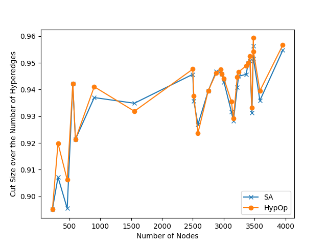
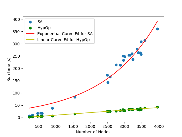
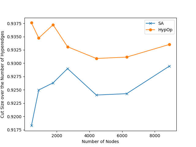
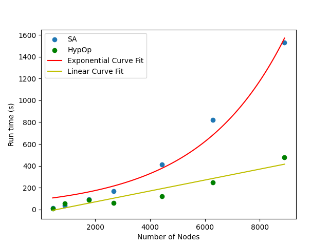
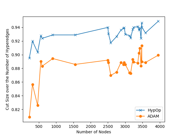
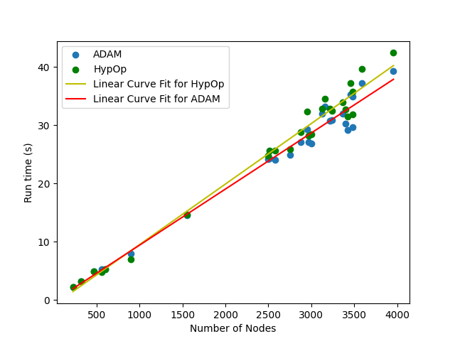
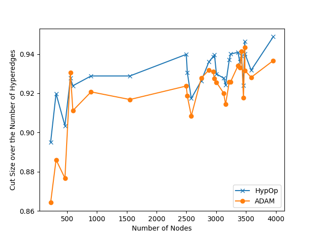
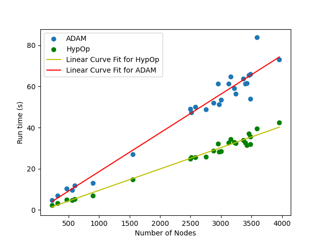
We use HypOp to solve the hypergraph MaxCut problem. In hypergraph MaxCut, the goal is to partition the nodes of a hypergraph into two groups such that the cut size is maximized, where the cut size is the number of hyperedges that have at least one pair of nodes belonging to different groups. We compare the performance of HypOp with simulated annealing and a direct gradient descent method (ADAM) as the baselines. Also, note that PI-GNN [36] can not solve problems over hypergraphs. We perform our experiments on both synthetic and real hypergraphs. The real hypergraphs are extracted from the the American Physical Society (APS) [1]. The APS dataset contains the basic metadata of all APS journal articles from year 1993 to 2021. Focusing on a specific journal within this dataset, Physical Review E (PRE), we partitioned the data into 3-year segments, and extracted the giant connected component of the authorship hypergraphs. The synthetic hypergraphs are generated randomly for some given specific values of number of nodes, edges, and upper bounds on the node degrees. For each synthetic hypergraph specifications, we generate 10 hypergraphs and the average results are reported. In Figures 3 and 4, we compare the performance of HypOp to SA for real (APS) and synthetic hypergraphs, respectively. We can see in Fig. 3 that with the same performance, the run time of HypOp grows linearly while the run time of SA grows exponentially with the number of nodes. Similar result is observed in Fig. 4 in terms of run time, while there is a huge performance gap between HypOp and SA. In Fig. 5, we compare the performance of HypOp with direct gradient descent using ADAM. As is evident in the figure, HypOp outperforms ADAM in both run time and performance.

(a) Performance of HypOp and SA

(b) Run time of HypOp and SA

Figure 3: Comparison between HypOp and SA for Hypergraph MaxCut problem on real hypergraphs extracted from APS dataset. With the same performance, the run time of SA grows exponentially while HypOp’s run time scales linearly.

(a) Performance of HypOp and SA

(b) Run time of HypOp and SA

Figure 4: Performance of HypOp compared with SA for hypergraph MaxCut problem on synthetic random hypergraphs. SA can not achieve performance similar to HypOp even with much longer run times that are growing exponentially fast, compared to run time of HypOp that grows linearly.

(a) Performance of HypOp and ADAM

(b) Run time of HypOp and ADAM

(c) Performance of HypOp and ADAM

(d) Run time of HypOp and ADAM

Figure 5: Comparison between HypOp and ADAM for hypergraph MaxCut problem on real hypergraphs extracted from APS dataset: (a) and (b): the same learning rate and number of epochs, and (c) and (d): double number of epochs for ADAM to improve its performance. ADAM can not achieve similar performance to HypOp even with twice number of epochs (twice run time).

VII-C SAT Problems

We have tested our algorithm on Random 3-SAT benchmarks from SATLIB dataset [16]. Table I shows the performance of HypOp on some of the satisfiable instances. We see that except for one with less than $2\%$ violation of constraints, all others were successfully solved. We provide our experiments on SAT problems to showcase the success of our algorithm on various problem instances, including the challenging and widely studied SAT problems. We need to note that we do not expect HypOp to compete with the powerful heuristics that are designed specifically for SAT problems and therefore, we do not provide any baselines in this section.

SAT Dataset	uf 20-91	uf 100-430	uf 200-860	uf 250-1065
Number of problems	100	100	100	100
Percentage Solved	$100\%$	$100\%$	$100\%$	$98\%$
Average number of unsatisfied clauses	0	0	0	1
Average time	4s	15s	37s	60s
Median time	4s	14s	21s	29s

Table I: Performance of HypOp on the SATLIB dataset. HypOp can solve SAT problems with linearly growing run time (median of run times for each dataset).

VII-D Maximum Independent Set Problem

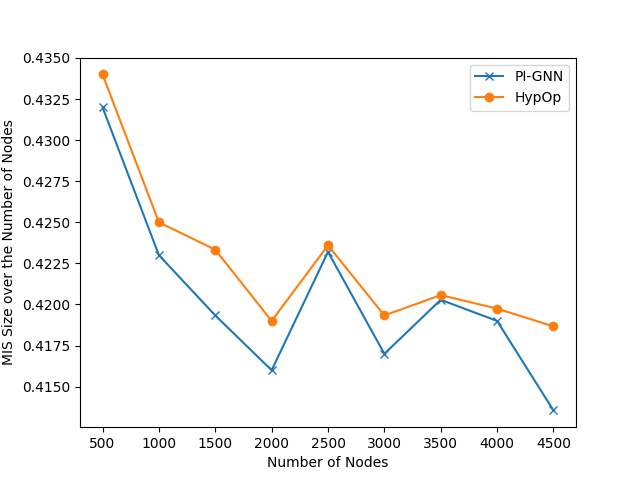
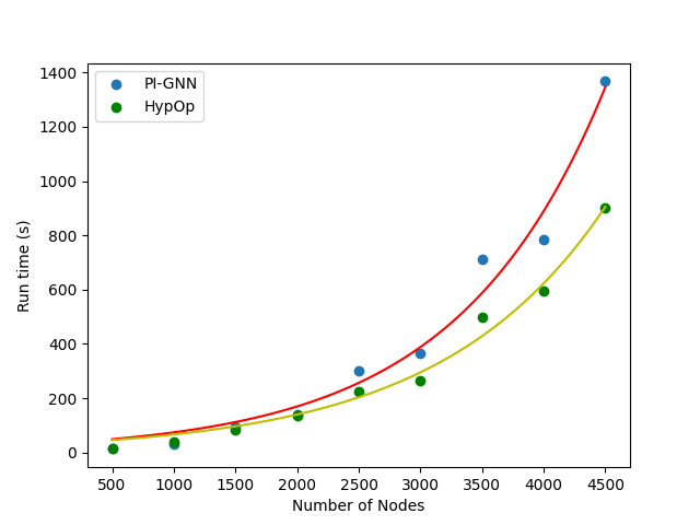
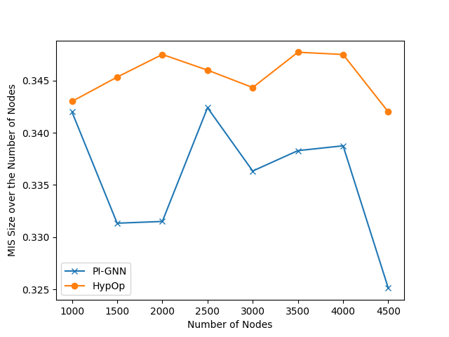
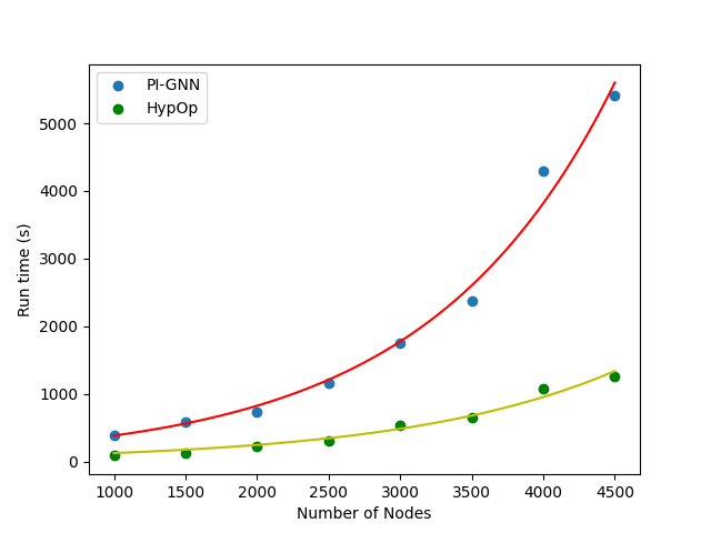
In order to compare HypOp with the baseline work PI-GNN [36] and highlight the benefit of the fine-tuning step using SA in HypOp, we also solved MIS problems over graphs using HypOp. We experimented on regular random graphs of different sizes with $d=3$ and $d=5$. In Fig. 6 and 7, we show the performance and run time of PI-GNN and HypOp over regular graphs with $d=3$ and $d=5$, respectively. As can be seen in the figures, HypOp performs better than PI-GNN both in terms of optimality and run time. Having different components in the optimization tool allows us to adjust the hyperparameters of them to better suit the specific problem at hand. Specially, we can have a more efficient algorithm by taking advantage of different types of solvers as is evident in our experimental results shown in Fig. 6 and 7. While generating better MIS sizes, the run time of HypOp is up to five times better than PI-GNN. HypOp also scales bettet than PI-GNN to larger graphs.

(a) MIS Ratio

(b) Run Time

Figure 6: Performance and run time of HypOp and PI-GNN for MIS problem on random regular graphs with $d=3$. HypOp achieves better results than PI-GNN in a less amount of time.

(a) MIS Ratio

(b) Run Time

Figure 7: Performance and run time of HypOp and PI-GNN for MIS problem on random regular graphs with $d=5$. HypOp achieves better results than PI-GNN in a significantly less amount of time.

VII-E Graph MaxCut

We have also considered graph MaxCut problems in order to be able to compare HypOp with the baseline solver [36] (PI-GNN). Similar to PI-GNN, we run HypOp on Gset dataset [43]. Table II summarizes our experiments on this dataset. As can be seen in the table, HypOp outperforms PI-GNN in all of the tested graphs.

We need to note here that Graph MaxCut is a very well studied problem and efficient heuristic algorithms have been developed to solve this problem. Although one can use algorithms such as HypOp and PI-GNN to solve MaxCut problems, these algorithms are not expected to outperform the efficient heuristics that are customized to the MaxCut problem specifics. However, the advantage of the learning-based algorithms such as HypOp and PI-GNN is that they are general solvers and one can use the same tool to solve thousands of optimization problems without the need to learn to run specific heuristics for each problem. So the main point of benchmarking HypOp on MaxCut problem is to compare its performance with the baseline algorithm PI-GNN and to further motivate the additional components that we have added to the baseline method.

Graph	G14	G15	G22	G49	G50	G55
Nodes	800	800	2000	3000	3000	5000
Edges	4694	4661	19990	6000	6000	12498
Run-CSP	2943	2928	13028	6000	5880	10116
PI-GNN	3026	2990	13181	5918	5820	10,138
HypOp	3042	3030	13185	5999	5879	10150
Best Known Result	3,064	3050	13359	6000	5880	10,294

Table II: Performance of HypOp on the Gset dataset. HypOp outperforms other unsupervised learning based methods, while achieving results that are close to the best known heuristics.

VII-F Resource Allocation Problem

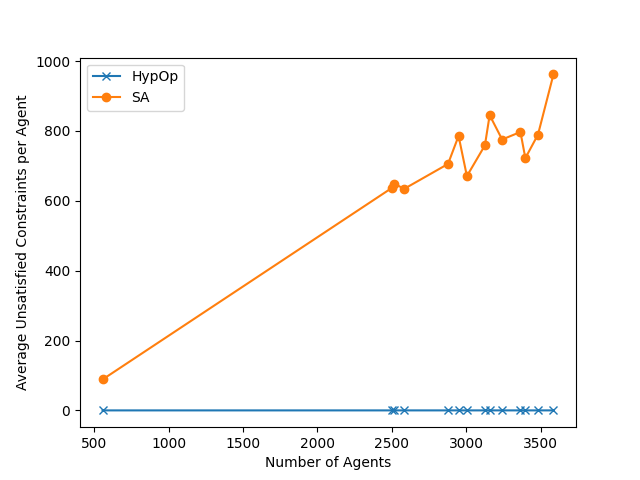
We use HypOp to solve a resource allocation problem where there are a number of tasks to be assigned to a number of agents with given energy and budget constraints. In particular, each agent has an energy budget to spend on the tasks and each task requires a minimum energy to be completed. We can also consider a global arbitrary objective function to minimize while satisfying the constraints. One can model this problem as a hypergraph discovery problem where the hypergraph nodes correspond to the agents and the hyperedges correspond to the tasks. The nodes (agents) within each hyperedge (task) are assigned to that task. One needs to discover different variations of this hypergraph to find feasible solutions and optimize the objective function. For simplicity, we do not consider a global objective function in our experiments and only try to find feasible solutions. In order to get realistic energy and budget constraints, we consider the APS co-authorship hypergraphs [1]. The papers correspond to tasks and the authors correspond to agents. The energy requirement of each task (paper) is the number of authors in it. Each agent has a budget that is a fixed number more than the papers that the agent appears in. We refer to this number as the budget surplus. The feasible set would be larger if we increase the budget surplus. We use the same budget surplus for all of the hypergraphs that we have considered so that as the number of agents in the hypergraph increases, the size of the feasible set shrinks. We use the initial co-authorship hypergraphs to build the HyperGNN in HypOp and try to find feasible solutions by assigning agents to tasks. We compare the result of HypOp with SA in Fig. 8. As can be seen in the figure, SA fails to find feasible solutions and its performance gets worse as the size of the feasible set shrinks (the number of agents increases). However, HypOp can find feasible solutions for all number of agents. Furthermore, in terms of run time, HypOp can solve these resource allocation problems in much less time than SA (87% less time).

Figure 8: Unsatisfied constraints in the Resource Allocation problem with different number of agents. HypOp can find feasible solutions (zero constraint violation), while SA fails to do so.

Table III: Average Run Time.

	Average Run Time (s)
HypOp	4668
SA	35472

VII-G Parallel and Distributed Training

In this section, we provide experimental results to verify the effectiveness of the scalable multi-GPU HyperGNN training described in algorithms 1 and 2. We solved MaxCut problem on one of the Stanford graphs, G22, in addition to a larger graph OGB-Arxiv [17] with 169343 nodes and 1166243 edges. The results are summarized in Table IV. For the smaller Stanford dataset (G22), the single GPU training and Algorithm 1 show similar performance with improved run time using Algorithm 1, while Algorithm 2 provides the outcome three times faster than the single GPU training. As the graph size becomes larger (OGB-Arxiv graph), single GPU training faces OOM (out of memory) error, whereas multi GPU training in HypOp can solve this problem. Algorithm 2 solves the problem almost two times faster than 1 with slight performance degradation ($\approx 0.1\%$ degradation).

Graph	Nodes	Edges	Single GPU		Centralized Multi-GPU		Distributed Multi-GPU
			Performance	Time	Performance	Time	Performance	Time
Stanford G22	2,000	19,990	13,185	15s	13,160	12s	13,128	5s
OGB-Arxiv	169,343	1,166,243	OOM	-	855,505	750s	854,746	411s

Table IV: Multi-GPU Performance. While Centralized Multi-GPU can speed up the optimization and resolve the OOM error, the distributed training provides significant speed up while its result is within 0.09% of the Centralized Multi-GPU result.

VIII Transfer Learning with HypOp for Different Types of Problems

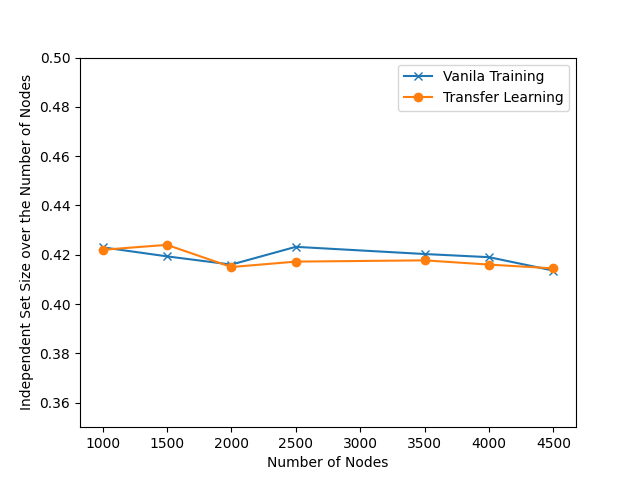
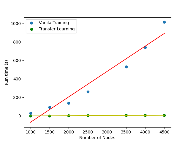
We explored the applicability of transfer learning within HypOp to address various problems on a single graph. Our approach involves pre-training the HyperGNN on a specific problem type and then utilizing the pre-trained model for a different optimization problem on the same graph, focusing on optimizing the input embedding exclusively. In particular, we freeze the weight matrix $W$ and only optimize on the input embedding $\sigma$. The underlying idea is that the HyperGNN learns an effective function to capture graph features (modeled by $\mathcal{G}(\sigma,w)$) and therefore, it can potentially be used for other types of optimization problems on the same graph. The optimization on the embedding $\sigma$ yields customized solutions tailored to the specific optimization problem type. To validate this, we trained the HyperGNN for the MaxCut problem and successfully transferred it to address the MIS problem.

In Fig. 9, we show the performance of HypOp with and without transfer learning on MIS problems on regular graphs with $d=3$. The models are pre-trained for MaxCut problem and transferred to solve MIS problem on the same graph. As we can see in the figure, the transferred model can achieve comparable results in almost no time compared to the vanilla training (training from scratch). This result further underscores the promising potential of utilizing unsupervised learning-based approaches to effectively and efficiently address complex optimization problems.

(a) Performance of HypOp with and without transfer learning.

(b) Run time of HypOp with and without transfer learning.

Figure 9: Transfer Learning using HypOp from MaxCut to MIS problem on random regular graphs with $d=3$. Similar result is obtained using Transfer Learning in almost no amount of time compared to Vanila training.

IX Applications in Scientific Discovery

Combinatorial optimization is a prevalent concept with applications spanning various fields in both science and industry. Decision-making in resource allocation, experimental design, task scheduling, and route selection often presents a multifaceted challenge in many areas of scientific discovery. Combinatorial optimization techniques can play a pivotal role in such scenarios by identifying optimal or nearly optimal solutions, thereby assisting in the decision-making process. In this section, we show an example of how HypOp can help with solving combinatorial optimization problems related to scientific discovery.

We consider a hypothetical experimental design by national drug control. We utilized a dataset that consists of the substances that make up drugs in the National Drug Code Directory maintained by the Food and Drug Administration [7]. This dataset, referred to as NDC dataset, consists of a list of drugs and the substances that make them. The drugs are considered as nodes and substances are presented by hyperedges. Drugs (nodes) within each hyperedge contain that substance. We considered the experiment of choosing a set of substances such that if one puts some regulatory measures on them, the rest of the dataset is divided into two separate (smaller) isolated group of drugs that can be addressed separately. We are interested to know the maximum number of substances that we need to regulate to create two separate datasets. This experiment can be represented by a hypergraph MaxCut problem on the NDC dataset and it can be solved using HypOp. Before applying HypOp on NDC dataset, We first removed the hyperedges containing one node and then we removed isolated nodes. As a result, we constructed a hypergraph with 3767 nodes and 29810 hyperedges. We applied HypOp on this hypergraph and the results are reported in Table V where we compare our result with SA. We can see that HypOp achieves better result in less time compared to SA.

	HypOp	Simulated Annealing
Cut Size	27776	27467
Run Time (s)	1601	2526

Table V: Performance of HypOp on NDC dataset. Compared to SA, HypOp can achieve better result in less amount of time.

X Limitations: Phase Transition in GNN Performance

Although learning-based approaches for optimization have shown tremendous potential, one has to be mindful of their limitations. In this section, we provide our experimental results on the performance of GNNs for MIS problems on various graphs. Note that for the analysis in this section, we consider the GNN outcome in HypOp with a simple threshold mapping as used in PI-GNN. For problems on graphs (including MIS), this will be the same as the PI-GNN result. We compare this result to the fine-tuned outcome generated by HypOp as an end-to-end solver. Our goal is to show the limitations of PI-GNN on some graphs. This analysis is inspired by the results of [25], where the authors study the limitations of the network online learning algorithms by considering different types of graphs.

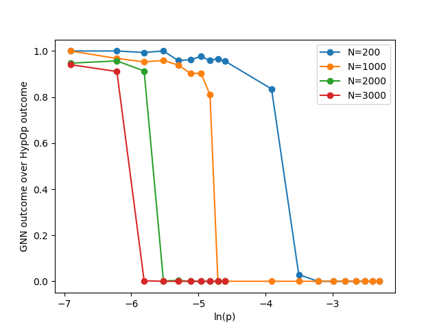
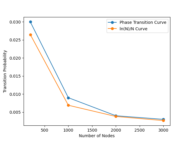
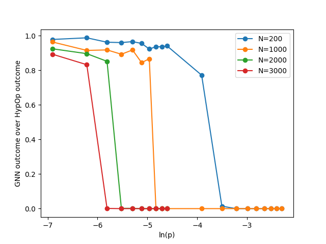
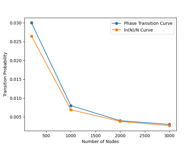
We investigated different structures of graphs, namely, Erdos-Renyi Random graphs, Regular graphs, and Powerlaw graphs (graphs with powerlaw degree distribution), with various options for their number of nodes and edges. We observed that for MIS problem, PI-GNN can not learn anything on the graphs that are denser than a given threshold. In Fig. 10(a) and 10(c), we show the performance of PI-GNN on Erdos-Renyi random graphs for different parameters, $p$, and different number of nodes, $N$, for two different learning rates. As is evident in the figure, the performance drops to 0 at a given threshold. The threshold, however, varies with the number of nodes. In Fig. 10(b) and 10(d), we show the plot of the phase transition threshold w.r.t. the number of nodes. The Erdos-Renyi graphs are well known for their phase transition in their connectivity. The threshold for this phase transition is $p^{*}=\frac{\text{ln}(N)}{N}$. As we have shown in Fig. 10(b) and 10(d), the phase transition threshold in the performance of PI-GNN is almost the same as the threshold for connectivity phase transition. This means that PI-GNN does not learn a solution over graphs that are dense enough to be connected. We provide our experimental results for two different learning rates to show that the performance drop is not caused by a high learning rate and is instead caused by the potential inability of GNNs to learn on dense graphs.

(a) Phase transition in the performance of PI-GNN over random graphs.

(b) Phase transition threshold w.r.t. the graph size, and comparison with the Erdos-Renyi graph connectivity phase transition, $p^{*}=\frac{ln(N)}{N}$.

(c) Phase transition in the performance of PI-GNN over random graphs.

(d) Phase transition threshold w.r.t. the graph size, and comparison with the Erdos-Renyi graph connectivity phase transition, $p^{*}=\frac{ln(N)}{N}$.

Figure 10: Phase transition in the GNN-based optimization performance for MIS problem with learning rate of $1e-4$ in (a) and (b) and learning rate of $1e-5$ in (c) and (d).

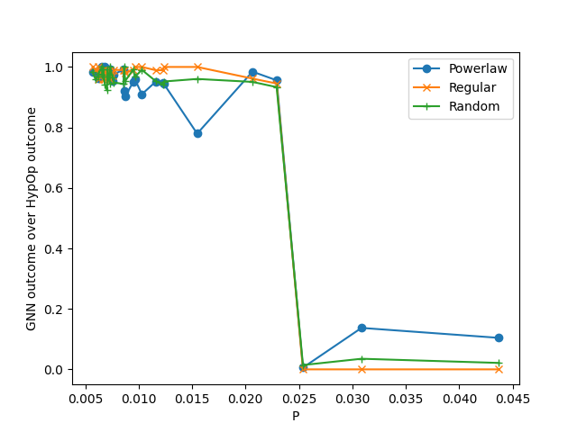
In order to investigate whether or not the specific structure of the graphs plays a role in the observed phase transition, we have compared the performance of PI-GNN on Powerlaw graphs, Regular graphs, and Random (Erdos-Renyi) graphs. In order to do the comparison, for each parameter of the powerlaw graphs, we construct random and regular graphs with almost the same number of edge density and compare the performance of PI-GNN over the three generated graphs. In Fig. 11, we show that the phase transition is the same for all of the three types of graphs when the performance is plotted w.r.t. the density ($p$) of the Random graph. Therefore, based on the existing evidence, we conclude that the performance is affected mainly by the density of the graph as opposed to its structure. We need to note here that most of the real graphs are powerlaw graphs with components between 2 to 4. Such graphs usually have lower densities than the observed critical density threshold for GNN learning.

Figure 11: Phase transition in the performance of PI-GNN for Powerlaw, Regular, and Erdos-Renyi graphs.

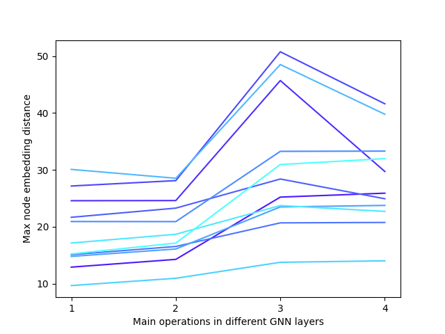
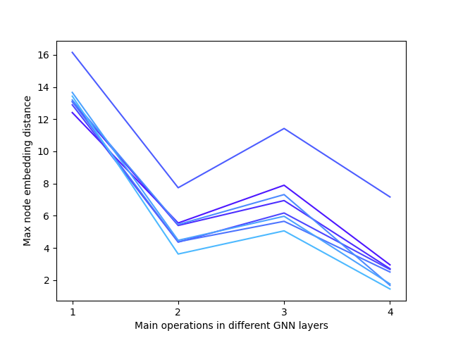
The phase transition in the GNN learning can be attributed to the oversmoothing issue that is widely observed in the GNNs throughout the literature [35]. Roughly speaking, oversmoothing occurs due to too many feature averaging, leading all hidden features to converge to the same point. In Fig. 12, we show the maximum distance between the output embeddings of the different nodes after the main operations of the HyperGNN (two convolutional and two aggregation operators). We provide two saparate figures, one for the graphs for which the PI-GNN is successful in producing good outcomes (graphs that have density less than the threshold found in Fig. 10), and one for the graphs for which the PI-GNN is not successful in producing good outcomes (graphs that are denser than the threshold found in Fig. 10). We see that the embedding distance is decreasing and converges to a small number for the dense graphs. This observation confirms the occurrence of oversmoothing in the HyperGNN training for dense graphs.

(a) Successful GNN training: graphs that are sparser than the phase transition threshold.

(b) Unsuccessful GNN training: graphs that are denser than the phase transition threshold.

Figure 12: Maximum node embedding distance after four main GNN operations. The plot is generated for MIS problem over random graphs with $N=200$. Oversmoothing is happening for graphs in (b) where the GNN training is unsuccessful.

A solution proposed in the literature for oversmoothing is graph sparsification by dropping edges [34]. This also explains how GNNs fail to learn good solutions on dense graphs as observed in Fig. 10. Motivated by [34], we propose graph sparsification to improve the GNN’s performance in HypOp.

X-A Graph Sparsification

With the observation that the inability of the GNNs to learn a good solution on some graphs is attributed to their high density, we explored the possibility of improving GNN learning through the process of graph sparsification. We experimented with the same graphs of Fig. 10 with $N=200$ nodes and sparsified the ones that the GNN failed to learn a good solution as follows. We remove each edge with a given probability $Ps$. A similar method was conducted in [34] to alleviate the oversmoothing issue in graph neural networks. We show the performance of HypOp on sparsified graphs with different values of $Ps$ in Fig. 13.

Figure 13: The performance of PI-GNN over original and sparsified random graphs with $N=200$ for MIS problem.

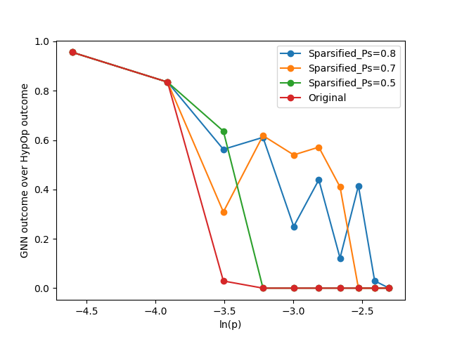
We can see in Fig. 13 that sparsification improves the performance of PI-GNN. However, there is still a gap between the overall outcome quality of HypOp and the outcome of the PI-GNN.

Based on our results in this section, we conclude that incorporating GNNs and HyperGNNs with other solvers has great advantages over using them as end-to-end solvers. This further motivates the fine-tuning step using SA that we have added in HypOp. This fine-tuning step can guarantee a good solution even if the GNN does not learn a good solution.

XI Discussion

XI-A Combining HyperGNN and SA

The comparison between HypOp and PI-GNN and SA in Section VII conveys two important messages that we would like to highlight here. First, utilizing unsupervised learning-based methods as an end-to-end optimization algorithm is not sufficient as it has been shown to have some limitations in some problems both in this work and in [2]. Combining such solvers with other generic optimization algorithms such as SA can significantly boost the performance of the algorithm and provide acceptable solutions even for the cases when the HyperGNN or GNN can not learn a good solution. Notice that SA has to only be run for a few iterations (30 $\sim$ 120). Second, HypOp and potentially other unsupervised learning-based optimization methods can act as an effective way to initialize the optimization variables in other solvers such as SA. As can be seen in our experiments, if SA is not initialized with the HyperGNN output in HypOp, it shows a much poorer performance compared to HypOp in terms of run time and performance.

XI-B Comparison with Direct Gradient Descent

As mentioned in Section V-B, in HypOp, HyperGNNs are used as learnable transformation functions that transform the input embedings into the original optimization variables. Gradient descent methods (such as ADAM) are then used to learn the parameters of the HyperGNN. However, one might ask why we do not directly use gradient descent to optimize over the original optimization variables. The answer is potentially related to the recent works on how neural networks can avoid local optima and find the global optima [10, 30]. Through our experiments in this paper, we showed the advantage of using HyperGNNs as transformation functions in the optimization process. Since gradient descent is a widely used tool in numerous areas, e.g., in ML for training neural networks, using HyperGNNs as transformation functions potentially can improve gradient descent-based optimization in many applications. In this paper, we provided some examples of the advantages of using HyperGNNs as transformation functions and we hope that in the future other applications would be introduced.

XI-C Effect of Self-Loops in the HyperGNN

It is common to add self-loops to the graphs before training a GNN on them. We observed that in HypOp (and similarly in PI-GNN), adding self loops will deteriorate the performance of the GNN or HyperGNN. The reason is most likely related to the results shown in in Section X where we showed that the GNNs fail to learn on graphs that are denser than a threshold. Adding self loops will make the graphs denser than is tolerated by the GNN, and therefore, we did not add self loops and also set the diagonal terms in the hypergraph adjacency matrix to 0 to create sparser graphs and hypergraphs.

XI-D Comparison with Bipartite Formulation

In this work, we used hypergraphs to model the constrained combinatorial optimization problems. An alternative option is utilizing bipartite graphs to model such problems. The bipartite graphs have two types of nodes: regular nodes and factor nodes. In a bipartite modeling of the constrained optimization problems, the regular nodes correspond to the variables (nodes in the hypergraph), and the factor nodes correspond to the constraints (hyperedges in the hypergraph). There is an edge from each node/variable to the factors/constraints that it appears in . One can see that every two message passing layers in the bipartite graph neural network can correspond to one layer of the hypergraph neural network. Therefore, we do not expect bipartite graph neural networks to perform vastly different from hypergraph neural networks in terms of the outcome quality. The only difference is that the number of nodes in the bipartite neural network modeling would be $N+K$, where $N$ is the number of variables and $K$ is the number of constraints, where the number of nodes in the hypergraph neural network modeling would be $N$. Since the run time and complexity of the graph and hypergraph neural networks scale with their number of nodes, hypergraph neural networks are the more efficient alternative compared to bipartite neural networks.

References

- [1] Aps data sets for research.
- [2] Maria Chiara Angelini and Federico Ricci-Tersenghi. Modern graph neural networks do worse than classical greedy algorithms in solving combinatorial optimization problems like maximum independent set. Nature Machine Intelligence, pages 1–3, 2022.
- [3] Mohammad Asghari, Amir M Fathollahi-Fard, SMJ Mirzapour Al-E-Hashem, and Maxim A Dulebenets. Transformation and linearization techniques in optimization: A state-of-the-art survey. Mathematics, 10(2):283, 2022.
- [4] Yunsheng Bai, Hao Ding, Song Bian, Ting Chen, Yizhou Sun, and Wei Wang. Simgnn: A neural network approach to fast graph similarity computation. In Proceedings of the twelfth ACM international conference on web search and data mining, pages 384–392, 2019.
- [5] Yoshua Bengio, Andrea Lodi, and Antoine Prouvost. Machine learning for combinatorial optimization: a methodological tour d’horizon. European Journal of Operational Research, 290(2):405–421, 2021.
- [6] Una Benlic and Jin-Kao Hao. Breakout local search for the max-cutproblem. Engineering Applications of Artificial Intelligence, 26(3):1162–1173, 2013.
- [7] Austin R. Benson, Rediet Abebe, Michael T. Schaub, Ali Jadbabaie, and Jon Kleinberg. Simplicial closure and higher-order link prediction. Proceedings of the National Academy of Sciences, 2018.
- [8] Quentin Cappart, Didier Chételat, Elias Khalil, Andrea Lodi, Christopher Morris, and Petar Veličković. Combinatorial optimization and reasoning with graph neural networks. arXiv preprint arXiv:2102.09544, 2021.
- [9] Chris Cummins, Pavlos Petoumenos, Zheng Wang, and Hugh Leather. End-to-end deep learning of optimization heuristics. In 2017 26th International Conference on Parallel Architectures and Compilation Techniques (PACT), pages 219–232. IEEE, 2017.
- [10] Simon Du, Jason Lee, Haochuan Li, Liwei Wang, and Xiyu Zhai. Gradient descent finds global minima of deep neural networks. In International conference on machine learning, pages 1675–1685. PMLR, 2019.
- [11] Alhussein Fawzi, Matej Balog, Aja Huang, Thomas Hubert, Bernardino Romera-Paredes, Mohammadamin Barekatain, Alexander Novikov, Francisco J R Ruiz, Julian Schrittwieser, Grzegorz Swirszcz, et al. Discovering faster matrix multiplication algorithms with reinforcement learning. Nature, 610(7930):47–53, 2022.
- [12] Song Feng, Emily Heath, Brett Jefferson, Cliff Joslyn, Henry Kvinge, Hugh D Mitchell, Brenda Praggastis, Amie J Eisfeld, Amy C Sims, Larissa B Thackray, et al. Hypergraph models of biological networks to identify genes critical to pathogenic viral response. BMC bioinformatics, 22(1):1–21, 2021.
- [13] Yifan Feng, Haoxuan You, Zizhao Zhang, Rongrong Ji, and Yue Gao. Hypergraph neural networks. In Proceedings of the AAAI conference on artificial intelligence, volume 33, pages 3558–3565, 2019.
- [14] Maxime Gasse, Didier Chételat, Nicola Ferroni, Laurent Charlin, and Andrea Lodi. Exact combinatorial optimization with graph convolutional neural networks. Advances in neural information processing systems, 32, 2019.
- [15] Ying He, Zheng Zhang, F Richard Yu, Nan Zhao, Hongxi Yin, Victor CM Leung, and Yanhua Zhang. Deep-reinforcement-learning-based optimization for cache-enabled opportunistic interference alignment wireless networks. IEEE Transactions on Vehicular Technology, 66(11):10433–10445, 2017.
- [16] Holger H Hoos and Thomas Stützle. Satlib: An online resource for research on sat. Sat, 2000:283–292, 2000.
- [17] Weihua Hu, Matthias Fey, Marinka Zitnik, Yuxiao Dong, Hongyu Ren, Bowen Liu, Michele Catasta, and Jure Leskovec. Open graph benchmark: Datasets for machine learning on graphs. Advances in neural information processing systems, 33:22118–22133, 2020.
- [18] Mojan Javaheripi, Mohammad Samragh, Tara Javidi, and Farinaz Koushanfar. Adans: Adaptive non-uniform sampling for automated design of compact dnns. IEEE Journal of Selected Topics in Signal Processing, 14(4):750–764, 2020.
- [19] Nikolaos Karalias and Andreas Loukas. Erdos goes neural: an unsupervised learning framework for combinatorial optimization on graphs. Advances in Neural Information Processing Systems, 33:6659–6672, 2020.
- [20] Elias Khalil, Pierre Le Bodic, Le Song, George Nemhauser, and Bistra Dilkina. Learning to branch in mixed integer programming. In Proceedings of the AAAI Conference on Artificial Intelligence, volume 30, 2016.
- [21] Diederik P Kingma and Jimmy Ba. Adam: A method for stochastic optimization. arXiv preprint arXiv:1412.6980, 2014.
- [22] Thomas N Kipf and Max Welling. Semi-supervised classification with graph convolutional networks. arXiv preprint arXiv:1609.02907, 2016.
- [23] Scott Kirkpatrick, C Daniel Gelatt Jr, and Mario P Vecchi. Optimization by simulated annealing. science, 220(4598):671–680, 1983.
- [24] Wouter Kool, Herke Van Hoof, and Max Welling. Attention, learn to solve routing problems! arXiv preprint arXiv:1803.08475, 2018.
- [25] Timothy LaRock, Timothy Sakharov, Sahely Bhadra, and Tina Eliassi-Rad. Understanding the limitations of network online learning. Applied Network Science, 5:1–25, 2020.
- [26] Bingjie Li, Guohua Wu, Yongming He, Mingfeng Fan, and Witold Pedrycz. An overview and experimental study of learning-based optimization algorithms for the vehicle routing problem. IEEE/CAA Journal of Automatica Sinica, 9(7):1115–1138, 2022.
- [27] Zhuwen Li, Qifeng Chen, and Vladlen Koltun. Combinatorial optimization with graph convolutional networks and guided tree search. Advances in neural information processing systems, 31, 2018.
- [28] Lu Liu, Yu Cheng, Lin Cai, Sheng Zhou, and Zhisheng Niu. Deep learning based optimization in wireless network. In 2017 IEEE international conference on communications (ICC), pages 1–6. IEEE, 2017.
- [29] Qiang Ma, Suwen Ge, Danyang He, Darshan Thaker, and Iddo Drori. Combinatorial optimization by graph pointer networks and hierarchical reinforcement learning. arXiv preprint arXiv:1911.04936, 2019.
- [30] Song Mei, Andrea Montanari, and Phan-Minh Nguyen. A mean field view of the landscape of two-layer neural networks. Proceedings of the National Academy of Sciences, 115(33):E7665–E7671, 2018.
- [31] Azalia Mirhoseini, Anna Goldie, Mustafa Yazgan, Joe Wenjie Jiang, Ebrahim Songhori, Shen Wang, Young-Joon Lee, Eric Johnson, Omkar Pathak, Azade Nazi, et al. A graph placement methodology for fast chip design. Nature, 594(7862):207–212, 2021.
- [32] Kevin A Murgas, Emil Saucan, and Romeil Sandhu. Hypergraph geometry reflects higher-order dynamics in protein interaction networks. Scientific Reports, 12(1):20879, 2022.
- [33] Vinod Nair, Sergey Bartunov, Felix Gimeno, Ingrid Von Glehn, Pawel Lichocki, Ivan Lobov, Brendan O’Donoghue, Nicolas Sonnerat, Christian Tjandraatmadja, Pengming Wang, et al. Solving mixed integer programs using neural networks. arXiv preprint arXiv:2012.13349, 2020.
- [34] Yu Rong, Wenbing Huang, Tingyang Xu, and Junzhou Huang. Dropedge: Towards deep graph convolutional networks on node classification. arXiv preprint arXiv:1907.10903, 2019.
- [35] T Konstantin Rusch, Michael M Bronstein, and Siddhartha Mishra. A survey on oversmoothing in graph neural networks. arXiv preprint arXiv:2303.10993, 2023.
- [36] Martin JA Schuetz, J Kyle Brubaker, and Helmut G Katzgraber. Combinatorial optimization with physics-inspired graph neural networks. Nature Machine Intelligence, 4(4):367–377, 2022.
- [37] Haoran Sun, Etash K Guha, and Hanjun Dai. Annealed training for combinatorial optimization on graphs. arXiv preprint arXiv:2207.11542, 2022.
- [38] Jan Toenshoff, Martin Ritzert, Hinrikus Wolf, and Martin Grohe. Graph neural networks for maximum constraint satisfaction. Frontiers in artificial intelligence, 3:580607, 2021.
- [39] Hanchen Wang, Tianfan Fu, Yuanqi Du, Wenhao Gao, Kexin Huang, Ziming Liu, Payal Chandak, Shengchao Liu, Peter Van Katwyk, Andreea Deac, et al. Scientific discovery in the age of artificial intelligence. Nature, 620(7972):47–60, 2023.
- [40] Yue Wen, Yue Gao, Shaohui Liu, Qimin Cheng, and Rongrong Ji. Hyperspectral image classification with hypergraph modelling. In Proceedings of the 4th International Conference on Internet Multimedia Computing and Service, pages 34–37, 2012.
- [41] Zonghan Wu, Shirui Pan, Fengwen Chen, Guodong Long, Chengqi Zhang, and S Yu Philip. A comprehensive survey on graph neural networks. IEEE transactions on neural networks and learning systems, 32(1):4–24, 2020.
- [42] Liqiao Xia, Pai Zheng, Xiao Huang, and Chao Liu. A novel hypergraph convolution network-based approach for predicting the material removal rate in chemical mechanical planarization. Journal of Intelligent Manufacturing, 33(8):2295–2306, 2022.
- [43] Y. Ye. The gset dataset (stanford, 2003).
- [44] Emre Yolcu and Barnabás Póczos. Learning local search heuristics for boolean satisfiability. Advances in Neural Information Processing Systems, 32, 2019.
- [45] Jianming Zhu, Junlei Zhu, Smita Ghosh, Weili Wu, and Jing Yuan. Social influence maximization in hypergraph in social networks. IEEE Transactions on Network Science and Engineering, 6(4):801–811, 2018.