Limits on Optical Counterparts to the Repeating FRB 20180916B from High-speed Imaging with Gemini-N/‘Alopeke

Abstract

We report on contemporaneous optical observations at $\approx 10$ ms timescales from the fast radio burst (FRB) 20180916B of two repeat bursts (FRB 20201023, FRB 20220908) taken with the ‘Alopeke camera on the Gemini North telescope. These repeats have radio fluences of 2.8 and 3.5 Jy ms, respectively, approximately in the lower 50th percentile for fluence from this repeating burst. The ‘Alopeke data reveal no significant optical detections at the FRB position and we place $3\sigma$ upper limits to the optical fluences of $<8.3\times 10^{-3}$ and $<7.7\times 10^{-3}$ Jy ms after correcting for line-of-sight extinction. Together, these yield the most sensitive limits to the optical-to-radio fluence ratio of an FRB on these timescales with $\eta_{\nu}<3\times 10^{-3}$ by roughly an order of magnitude. These measurements rule out progenitor models where FRB 20180916B has a similar fluence ratio to optical pulsars similar to the Crab pulsar or optical emission is produced as inverse Compton radiation in a pulsar magnetosphere or young supernova remnant. Our ongoing program with ‘Alopeke on Gemini-N will continue to monitor repeating FRBs, including FRB 20180916B, to search for optical counterparts on ms timescales.

1 Introduction

More than a decade has passed since fast-radio bursts (FRBs) were discovered (Lorimer et al., 2007), and it is now well established that they are emitted by extragalactic, astrophysical sources (e.g. Cordes & Chatterjee, 2019; Zhang, 2020). However, the stellar systems, their configuration, and the exact physical mechanism(s) capable of releasing radio pulses required by FRB energies ($\sim 10^{40}$–$10^{43}$ erg) and short timescales ($\sim 10^{-3}$ s) remain elusive.

Several theories have been proposed for the origin of FRBs (see Petroff et al., 2022, for a review), although many of these are already ruled out for the bulk of the FRB population (Bhandari et al., 2020; Heintz et al., 2020; Marnoch et al., 2020; Gordon et al., 2023). The current prevailing view is that they may be related to eruptions from magnetars based on the detection of a low-energy FRB from the Galactic magnetar SGR 1935+2154 (Bochenek et al., 2020b; CHIME/FRB Collaboration et al., 2020). However, the magnetar theory is complicated by evidence for periodicity in some FRBs (Chime/Frb Collaboration et al., 2020; Rajwade et al., 2020, whereas magnetar eruptions are more likely to be stochastic) and the detection of a repeating FRB in a globular cluster with an extremely old stellar population (Kirsten et al., 2022). Curiously, the FRB signal from SGR 1935+2154 was accompanied by a simultaneous detection of a hard X-ray emission by INTEGRAL and Konus-WIND, suggesting a broadband, non-thermal emission model (Mereghetti et al., 2020; Ridnaia et al., 2021). Even in the specific case in which FRBs arise from magnetar eruptions, various models predict broadband, multi-wavelength emission via an afterglow from a synchrotron maser (Waxman, 2017; Metzger et al., 2019; Margalit et al., 2020), coherent curvature radiation from charged particles in the magnetic field (Kumar et al., 2017; Ghisellini & Locatelli, 2018; Katz, 2018; Yang & Zhang, 2018), or inverse Compton scattering of FRB photons to optical wavelengths (Zhang, 2022). A key component of most of these theories is that the optical signal will be both simultaneous with and have a similar timescale to the FRB, producing a so-called fast optical burst (FOB; see, e.g., Karpov et al., 2019; Yang et al., 2019).

Unlike the heterodyne receivers that can detect FRBs as voltages sampled with variable time resolution down to microseconds or even faster (Day et al., 2020), the vast majority of optical detectors operate with a fundamental limit on their exposure times of a few seconds, mostly driven by readout time and shutter speed (e.g., Ivezić et al., 2019). This presents a challenge for detecting optical counterparts to FRBs with timescales of milliseconds, although sensitive, wide-field surveys such as the Vera C. Rubin Legacy Survey of Space and Time may detect several dozen with proper filtering of their transient alerts (Megias Homar et al., 2023).

Targeted follow up of FRBs with high-speed optical cameras such as electron multiplying CCDs (Scott & Howell, 2018) offers a better strategy for constraining optical emission with a duration of milliseconds. By observing FRBs during periods of high activity (e.g., repeating FRBs with known periods or FRBs undergoing “burst storms” with hundreds of events over hours or days; Fonseca et al., 2020; Fong et al., 2021; Ravi et al., 2022), we can maximize the likelihood that an optical facility is observing a FRB when a radio burst is detected. This strategy has been implemented by several groups for FRB 20121102A (MAGIC Collaboration et al., 2018), FRB 20180916B (Kilpatrick et al., 2021), and FRB 20201124A (Piro et al., 2021) among others, including high-speed optical camera observations of FRB 20121102A by Hardy et al. (2017) and FRB 20180916B by Pilia et al. (2020). However, in both cases these observations were relatively shallow, limited by the aperture size of the telescopes used (1.2–2.4 m) and conditions at the observing sites.

Here we present results from an observing campaign of the periodic, repeating FRB 20180916B with the ‘Alopeke high-speed camera on the 8.1 m Gemini-North telescope at Maunakea, Hawaii. By targeting the FRB during expected periods of high activity and during the transit window when it was observable by CHIME, we obtained two observations simultaneous with radio bursts. Our observing strategy, data reduction, and calibration is described in Section 2. We describe our analysis of the data and limits on an optical counterpart to the radio bursts in Section 3 and the implications for optical analogs, counterpart models, and prospects for future high-speed optical observations of FRBs in Section 4. Finally, we conclude in Section 5.

Throughout this paper, we assume a luminosity distance to FRB 20180916B of 150 Mpc from Marcote et al. (2020) and Chime/Frb Collaboration et al. (2020) and a Milky Way reddening to FRB 20180916B of $E(B-V)=0.87$ mag (Schlafly & Finkbeiner, 2011).

2 Data and Calibration

2.1 CHIME Radio Detection

CHIME detected bursts from FRB 20180916B as it was transiting at UTC 2020-10-23 07:48:30.778 and UTC 2022-09-08T10:53:26.889, which is confirmed by the dispersion measure (DM) from both events 350.5 and 349.9 pc cm^-3, respectively, compared with the average DM of 349.2 pc cm^-3 (Figure LABEL:fig:detection and CHIME/FRB Collaboration et al., 2019; Marcote et al., 2020). The consistency in sky localization and DM-space rules out the possibility of chance coincidence from another burst.

The basic burst properties from FRB 20201023 and FRB 20220908 were derived using the fitburst codebase (Fonseca et al., 2023). These bursts have durations of $t_{\rm radio}=$2.7$\pm$0.3 ms and 2.7$\pm$0.2 ms, peak flux of $f_{\nu,{\rm radio}}=$0.5$\pm$0.2 Jy and 0.5$\pm$0.2 Jy, and fluence of $F_{\rm radio}=$2.6$\pm$0.8 Jy ms and 3.5$\pm$0.8 Jy ms, respectively. As with all CHIME bursts (e.g., those in the CHIME DR1 FRB catalog; CHIME/FRB Collaboration et al., 2021), the dispersion-corrected arrival time is calculated at a rest frequency of 400.19 MHz, which we assume below for comparison to our optical data.

2.2 ‘Alopeke High-speed Imaging

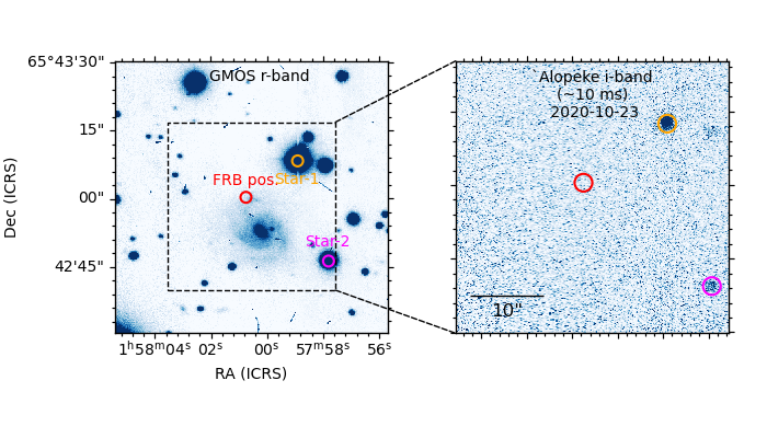
Figure 2: Left: Portion ($\sim 1\arcmin\times 1\arcmin$) of Gemini GMOS $z$-band image from Marcote et al. (2020) centered on FRB 20180916B. The FRB position (red) and nearby reference stars (Star-1; orange, Star-2; purple) are labeled. Right: Field-of-view of ‘Alopeke ($37\arcsec\times 37\arcsec$) around the FRB 20180916B position. Only the Star-1 and Star-2 are detected in a single 10.419 ms exposure.

We contemporaneously observed the FRB 20180916B field with the ‘Alopeke high-cadence camera (Scott & Howell, 2018; Scott et al., 2021) as part of Gemini-N programs GN-2020B-DD-103 and GN-2022B-Q-202 (PI Prochaska). Observations were carried out on UTC 2020-10-23 and 2022-09-08 using ‘Alopeke’s wide-field mode with $2\times 2$ binning in a region of $256\times 256$ pixels around the FRB position. This provides an effective field-of-view of $37\arcsec\times 37\arcsec$, a pixel scale of $0.145\arcsec~{}{\rm pixel}^{-1}$, and a time resolution of 10.419 ms.

We coordinated the ‘Alopeke observations to coincide with the CHIME transit at the expected peak of the $\sim$$16.3$ day periodic activity of the repeater FRB 20180916B (Chime/Frb Collaboration et al., 2020). We observed the field for $\approx$1136 s almost continuously in the $r$ and $i$ bands starting at UT 2020-10-23T07:41:40.265 and for $\approx$1315 s starting at 2022-09-08T10:39:04.629. These $r$ and $i$-band exposures were observed near simultaneously using the blue and red cameras, respectively. In each camera and exposure, we obtained $5000$ individual exposures of 10.419 ms each (with accumulation cycle time of 11.595 ms), where each set lasted for $\sim 1$ min including read-out overhead. There were 20 separate exposures per camera on 2020-10-23 and 23 separate exposures per camera on 2022-09-08.

Our observing strategy covered time-frames approximately $\approx 10$–$12$ min before and after the peak of the CHIME transit on each date. As we observed on a date near the peak of the FRB 20180916B activity cycle, this maximized the likelihood of observing at a time when CHIME was likely to detect a radio burst.

After science observations on each night, a series of $3$ flat field calibrations were taken for each camera, with the exact same setup ($5000$ exposures per series), using the twilight sky as reference. A set of $2$ bias/dark series observations were also taken after science observations on the same day. Given the short exposure times, bias and darks are essentially the same and we combined them together to produce a “master bias.”

We reduced all of our imaging with using custom software implementing astropy (Bradley et al., 2022). Master bias, dark, and flat images were created for both cameras and filters (i.e., the blue, $r$-band and red, $i$-band, respectively) by combining the individual exposures of the individual bias frames and flat frames. We obtained an individual reduced image by subtracting the corresponding master bias to each individual frame, and by dividing the result by the corresponding normalized master flat.

The field-of-view of the observations in both epochs is centered at the FRB position, and every exposures contains at least two point-like sources that are classified as stars in the Pan-STARRS catalog (Chambers et al., 2016a) and are bright enough to be well detected in the individual 10.419 ms exposures. We used these two stars to define both the absolute astrometric and photometric calibration across all 5000 frames individually for every exposure. Comparing to an overlapping, wider Gemini-N/GMOS image (Marcote et al., 2020), the two stars are well aligned to this much deeper frame. We refer to the brightest star in the field-of-view (Pan-STARRS objID=186860294956243663; Chambers et al., 2016a; Flewelling et al., 2020) as Star-1 and the second brightest star (objID=186850294911316323) as Star-2 throughout the manuscript.

2.3 Astrometry

For absolute astrometry, we used the positions of Star-1 ($\alpha=29.495612$, $\delta=65.719111$) and Star-2 ($\alpha=29.491117$, $\delta=65.712993$) (Gaia Collaboration et al., 2018; Lindegren et al., 2018) to set the alignment and rotation of the ‘Alopeke camera, assuming zero distortion and an absolute pixel scale of $0.145\arcsec\,\rm pixel^{-1}$ across the entire detector. This alignment strategy yields good results when comparing the stacked 5000 frames for each exposure to the deeper GMOS observation where we detect at least 5 point sources in the stacked frames. We obtain $\sim$0.1″ root-mean square offsets in both right ascension and declination between the stacked ‘Alopeke data and the GMOS image. Figure 2 shows a GMOS $z$-band image ($\sim 1\arcmin\times 1\arcmin$; left panel) and a single ‘Alopeke $i$-band image ($37\arcsec\times 37\arcsec$; right panel) around the FRB position. The seeing was approximately 0.5″ in the first epoch and 0.8″ in the second epoch and we perform photometry within 2 FWHM of the FRB location, so we are confident that astrometric uncertainty does not significantly affect our analysis.

2.4 Time calibration and sensitivity

The ‘Alopeke time stamps for each of the 5000$\times$10.4 ms exposures are given by the Network Time Protocol (NTP) from UTC times. Its absolute time accuracy is $160\pm 0.07$ ms (see, e.g., Scott & Howell, 2018; Scott et al., 2021), mostly driven by the variable lag between the computer receipt from the NTP server and the triggering of the cameras. This sets our primary source of time calibration uncertainty. We note, however, that the relative time accuracy between individual 10.4 ms frames in the ‘Alopeke exposures is much smaller ($\sim 70$ ns), and thus we ignore them.

CHIME operates with a time resolution of 0.983 ms (CHIME/FRB Collaboration et al., 2018; Chime/Frb Collaboration et al., 2020), and the uncertainty on the arrival time at infinite frequency for each burst (mjd_inf_err) is typically 0.5–2 ms. Compared with the uncertainty in the time accuracy for CHIME, we consider this to be a negligible uncertainty.

The topocentric FRB pulse time arrival at $400$ MHz was UTC 2020-10-23 07:48:30.778. This implies that any putative optical counterpart should have arrived $9.083$ s earlier, that is, at UTC 2020-10-23T07:48:21.695 based on the arrival time at infinite frequency for a radio signal detected at 400 MHz and dispersion measure of 350.19 pc cm^-3 (Figure LABEL:fig:detection) using equation 1 of Cordes & Chatterjee (2019). Considering the rapid timescales involved in this calculation, we also consider the light-travel time between ‘Alopeke and CHIME, which are located on Maunakea, Hawaii and Penticton, BC, Canada, respectively, separated by a direct distance of 4470 km. This corresponds to a maximum difference in arrival times for a signal at infinity frequency of 14.9 ms between ‘Alopeke and CHIME. We targeted FRB 20180916B when it was transiting over CHIME, and at the arrival time at infinite frequency, it was at an hour angle 57 s east of CHIME. This implies that the same signal would arrive approximately the full 14.9 ms light-travel time later in Hawaii, and so we assume the arrival of the signal was UTC 2020-10-23T07:48:21.709 for ‘Alopeke.

We performed the same analysis for the 2022-09-08 burst, which was detected by CHIME at an arrival time of UTC 2022-09-08T10:53:26.889. The dispersion measure of 349.8 pc cm^-3 implies that at infinite frequency this burst arrived at the CHIME radio array at UTC 2022-09-08T10:53:17.817. Given that the burst was at an hour angle 5 minutes and 3 seconds west of CHIME at this time and 2 hours, 18 minutes, and 21 seconds east of Maunakea, we estimate that the optical signal would arrive ‘Alopeke the full 14.3 ms later at UTC 2022-09-08T10:53:17.831. For both bursts, we take the ‘Alopeke data around the corresponding arrival times calculated here to search for optical emission associated with the radio bursts, but we consider a $\pm$160 ms range of data to account for the absolute uncertainty in the ‘Alopeke time stamps.

Finally, considering the cadence of $11.6$ ms and the actual individual exposure time of 10.4 ms there is in principle the possibility that the putative optical pulse associated with the FRB arrived in between individual exposures. However, the “down-time” of the ‘Alopeke camera in our current setup of $\sim 6\%$ is sufficiently small allowing us to be sensitive to pulses wider than 1 ms. Moreover, even for pulses intrinsically narrower than this, the fact that we are using two cameras at slightly different starting times make it very unlikely to miss a pulse in both of them.

2.5 Flux Calibration

We perform aperture photometry in the ‘Alopeke data relative to Star-1 and Star-2. The apparent magnitudes of these reference stars are $r=15.7481\pm 0.0030$ mag and $i=15.1387\pm 0.0069$ mag for Star-1 and $r=17.1016\pm 0.0225$ mag and $i=16.6247\pm 0.0121$ mag for Star-2 obtained from Pan-STARRS1 (Chambers et al., 2016b). In the following photometric analysis, we use the count rate of both stars to set the absolute flux scale for each frame. Based on the Galactic reddening assumed above, we further correct our photometry for line-of-sight extinction of $A_{r}=2.2\,{\rm mag}$ and $A_{i}=1.5$ mag.

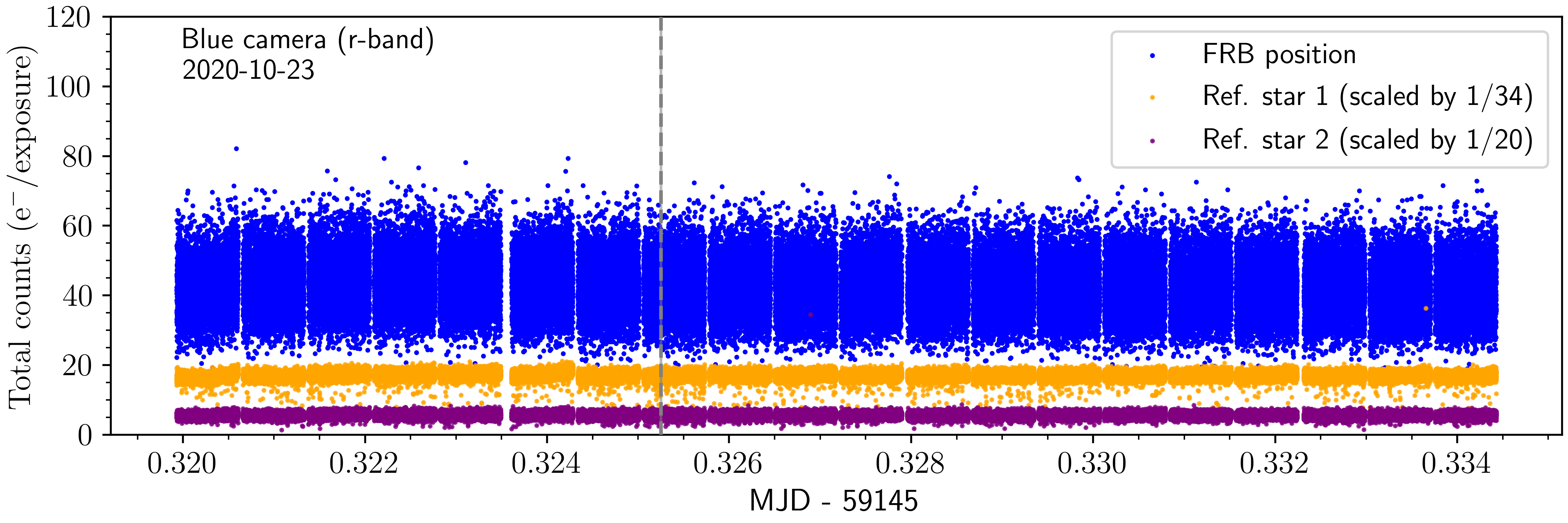
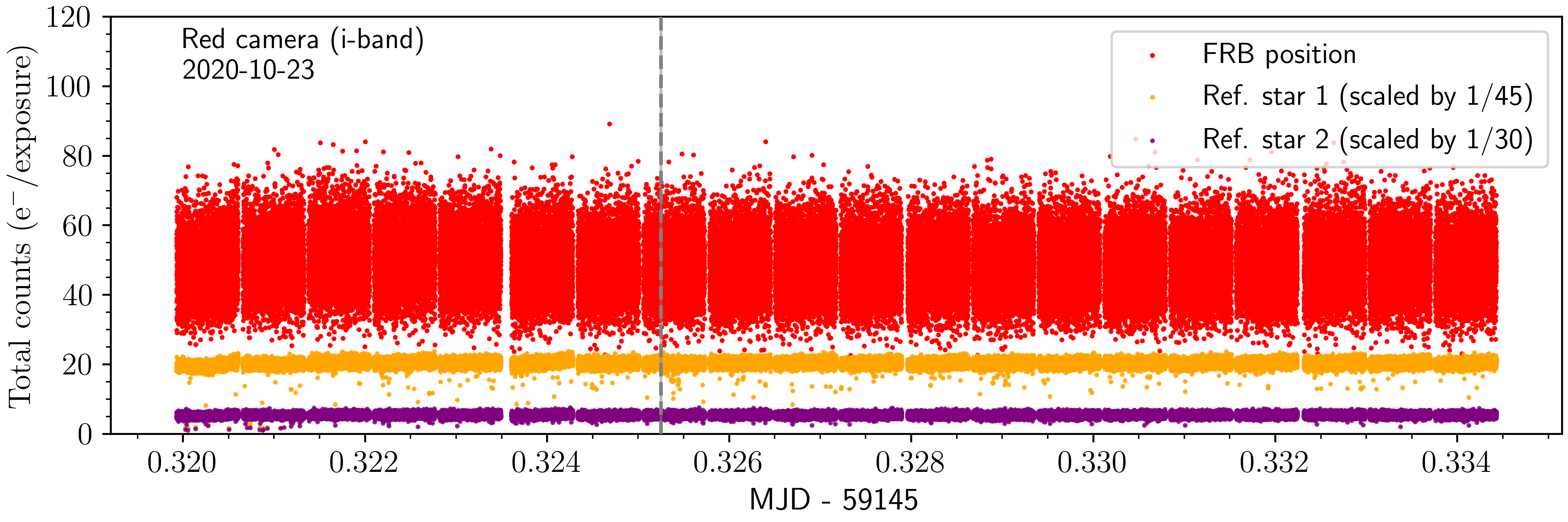
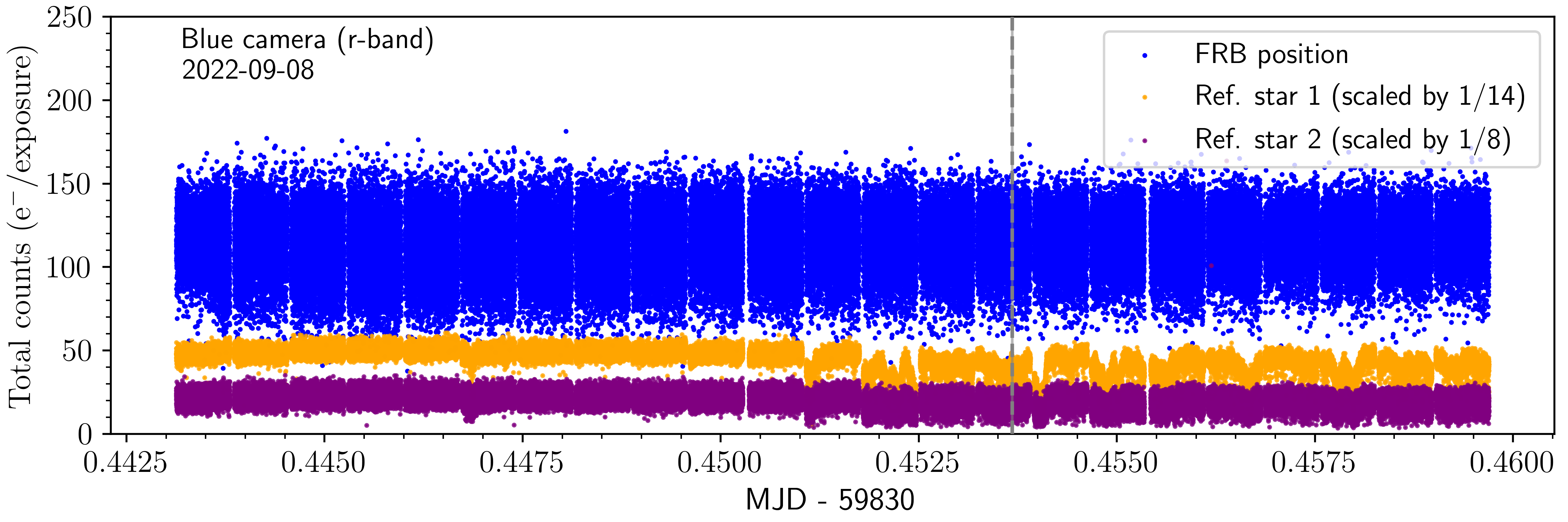
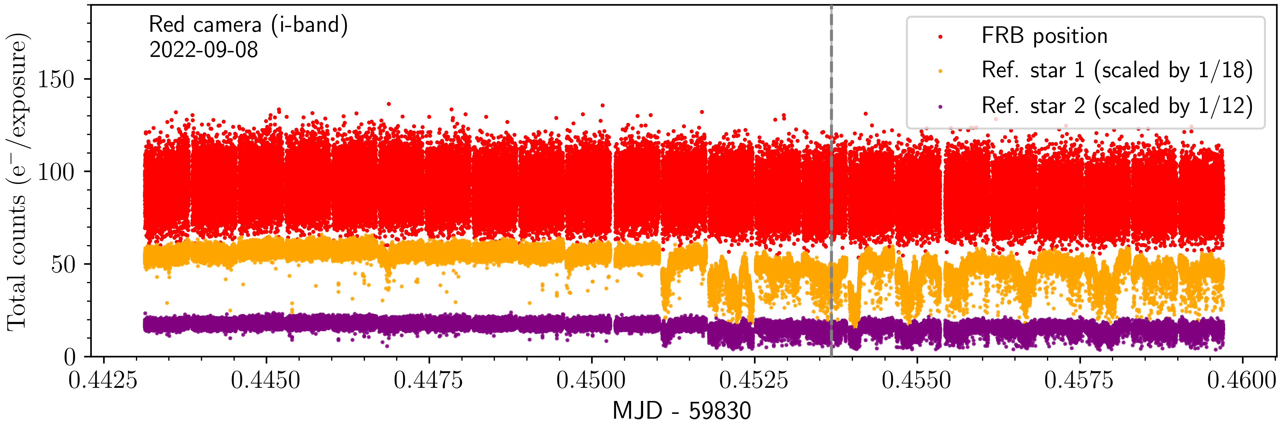
Figure 3: Top two panels: Total count rate (e^-/exposure) at the FRB location using a circular aperture with radius of two FWHM assessed from Star-1 and Star-2. Counts for the blue camera are shown in the top panel while those for the red camera are shown in the bottom panel. Each panel also show the respective counts of the reference star scaled by a constant factor. The count-rates show a small drift towards lower values across the observing period of $\approx 750$ s. The regular gaps arise due to read-out of the detectors. Noticeable variation in the count level are also seen in the reference star, thus indicating they may be telluric. Any optical emission from the FRB 20180916B is predicted arrive at ‘Alopeke at MJD = 59145.32525072763 (Section 2.4) marked by the dashed vertical lines. Bottom two panels: Same as the top panels for the second CHIME event we observed from FRB 20180916B. Conditions were not photometric, as shown by the variable flux from Star-1 and Star-2. The dashed line indicates the time of the burst at MJD = 59830.45367810875.

Table 1: Photometry for Blue Camera ($r$-band)

MJD	$C_{\rm bkg}$	$C_{\rm Star-1}^{\rm Tot}$	$C_{\rm Star-2}^{\rm Tot}$	$C_{\rm FRB}^{\rm Tot}$
59145.32525183	53.95	629.68	134.18	53.11
59145.32525169	33.14	593.92	119.27	31.15
59145.32525156	54.34	593.81	103.40	40.30
59145.32525142	45.39	639.92	107.57	33.92
59145.32525129	36.45	637.76	114.95	42.32
59145.32525115	31.10	631.27	127.16	35.86
59145.32525102	34.27	600.15	124.73	51.80
59145.32525088	45.23	688.93	118.49	38.60
59145.32525075	58.60	222.24	68.41	51.86
59145.32525062	59.28	604.63	111.40	55.51
59145.32525048	38.98	652.59	108.91	36.53
59145.32525035	49.33	649.81	124.12	45.42
59145.32525021	38.35	581.59	112.30	54.41
59145.32525008	45.60	615.87	117.90	44.30
59830.45367901	117.72	722.42	208.14	94.63
59830.45367888	141.90	775.88	251.05	117.41
59830.45367874	101.42	718.38	161.78	132.69
59830.45367861	134.09	675.11	154.49	90.93
59830.45367848	96.41	687.47	164.43	133.75
59830.45367834	118.88	697.87	191.42	130.06
59830.45367821	126.88	714.53	158.47	127.82
59830.45367807	92.48	654.53	173.02	124.73
59830.45367794	103.90	686.17	169.42	133.45
59830.45367781	131.40	703.54	184.31	93.70
59830.45367767	144.47	690.74	169.79	119.77
59830.45367754	89.00	696.97	149.41	122.43
59830.45367740	102.38	765.27	161.21	107.02
59830.45367727	77.70	668.95	160.54	130.89

Table 2: Photometry for Red Camera ($i$-band)

MJD	$C_{\rm bkg}$	$C_{\rm Star-1}^{\rm Tot}$	$C_{\rm Star-2}^{\rm Tot}$	$C_{\rm FRB}^{\rm Tot}$
59145.32525190	56.38	968.71	162.36	39.78
59145.32525176	48.62	943.33	157.73	36.48
59145.32525163	44.47	937.69	181.28	53.24
59145.32525149	52.45	986.96	159.19	43.93
59145.32525136	46.44	982.17	153.60	38.64
59145.32525122	45.74	921.25	161.28	50.57
59145.32525109	46.11	1011.73	178.21	45.82
59145.32525095	49.06	953.44	183.01	72.33
59145.32525082	56.08	934.66	173.28	44.09
59145.32525069	46.95	939.67	174.52	45.19
59145.32525055	71.07	983.18	168.23	42.54
59145.32525042	62.22	1042.15	193.04	55.64
59145.32525028	52.06	926.46	144.29	55.04
59145.32525015	49.63	939.32	160.76	34.23
59830.45367898	102.55	1026.24	254.88	97.34
59830.45367885	96.79	1031.09	227.96	73.23
59830.45367872	88.02	1018.30	204.55	98.24
59830.45367858	81.72	1020.87	218.72	94.50
59830.45367845	86.83	1089.42	250.15	96.88
59830.45367831	85.25	1034.26	207.45	76.77
59830.45367818	85.08	1093.24	240.30	95.13
59830.45367804	88.20	1086.52	205.34	87.05
59830.45367791	102.85	1065.19	224.98	90.81
59830.45367777	100.17	1064.64	225.16	94.77
59830.45367764	96.77	995.53	233.08	96.39
59830.45367750	91.61	1047.45	208.60	94.72
59830.45367737	66.93	1053.33	199.60	76.86
59830.45367724	92.91	1007.54	261.67	76.40

3 Photometric Analysis

In this section we describe the analysis related to photometric measurements from the ‘Alopeke imaging, including our measurements of the count rate and upper limits on the count rate at the site of FRB 20180916B within each $\sim$10.4 ms frame.

3.1 Count-rate Measurements

In each camera and for each exposure we first measured the centroid and full-width at half-maximum (FWHM) for reference Star-1 and Star-2. We then measured the count rates of these stars within an aperture of diameter 2 FWHM and then the counts in the same sized aperture at the location of FRB 20180916B.

Our final count-rate measurements are tabulated in Table 1 and 2 for the closest $\approx$163 ms to the arrival time of FRB 20201023 and FRB 20220908. These counts include all sources of photoelectrons: the night sky, the galaxy hosting FRB 20180916B, the detector, and the individual sources of interest. We refer to count-rates at the Star-1, Star-2, and at the location of FRB 20180916B as $C_{\rm Star-1}^{\rm Tot}$, $C_{\rm Star-2}^{\rm Tot}$, and $C_{\rm FRB}^{\rm Tot}$, respectively. Our final results will be derived from departures (or lack thereof) from the mean of $C_{\rm FRB}^{\rm Tot}$. For comparison, we also estimate the local background count-rate near Star-1 by measuring the counts per frame and pixel in an annulus with inner radius 3 FWHM and outer radius 6 FWHM and rescaling the total count rate to the size of the 2 FWHM.

3.2 Constraints on a Counterpart to FRB 20180916B and Flux Limits

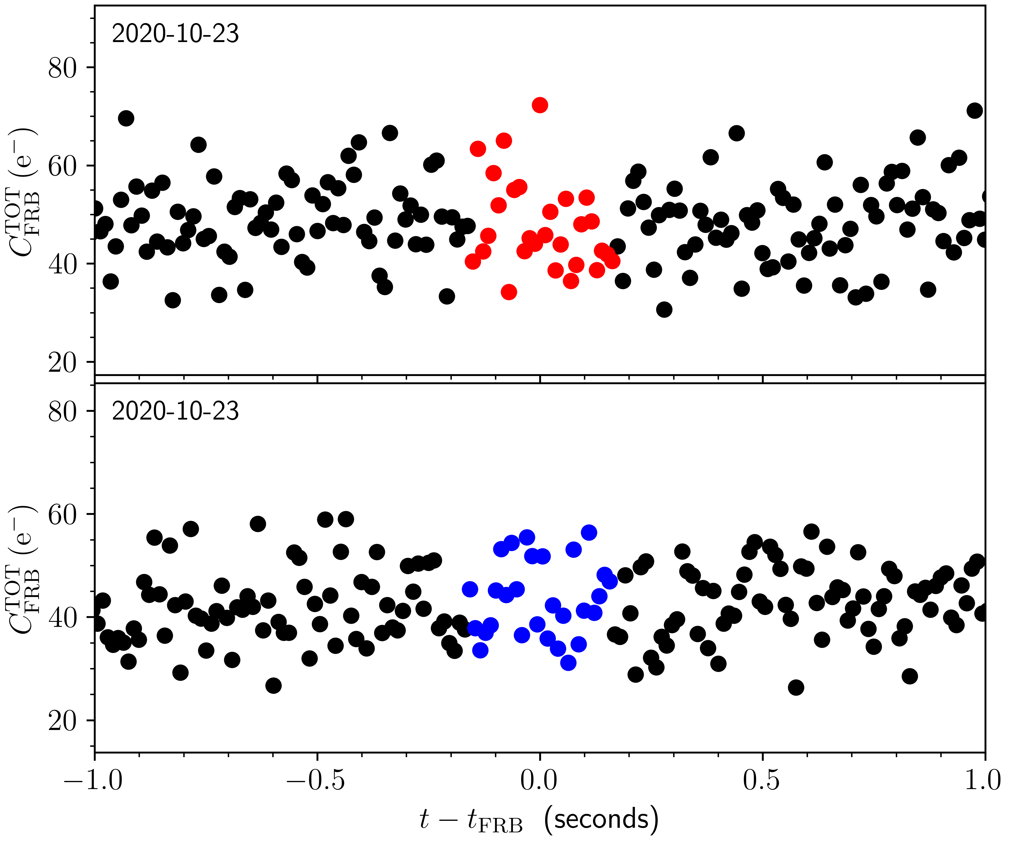
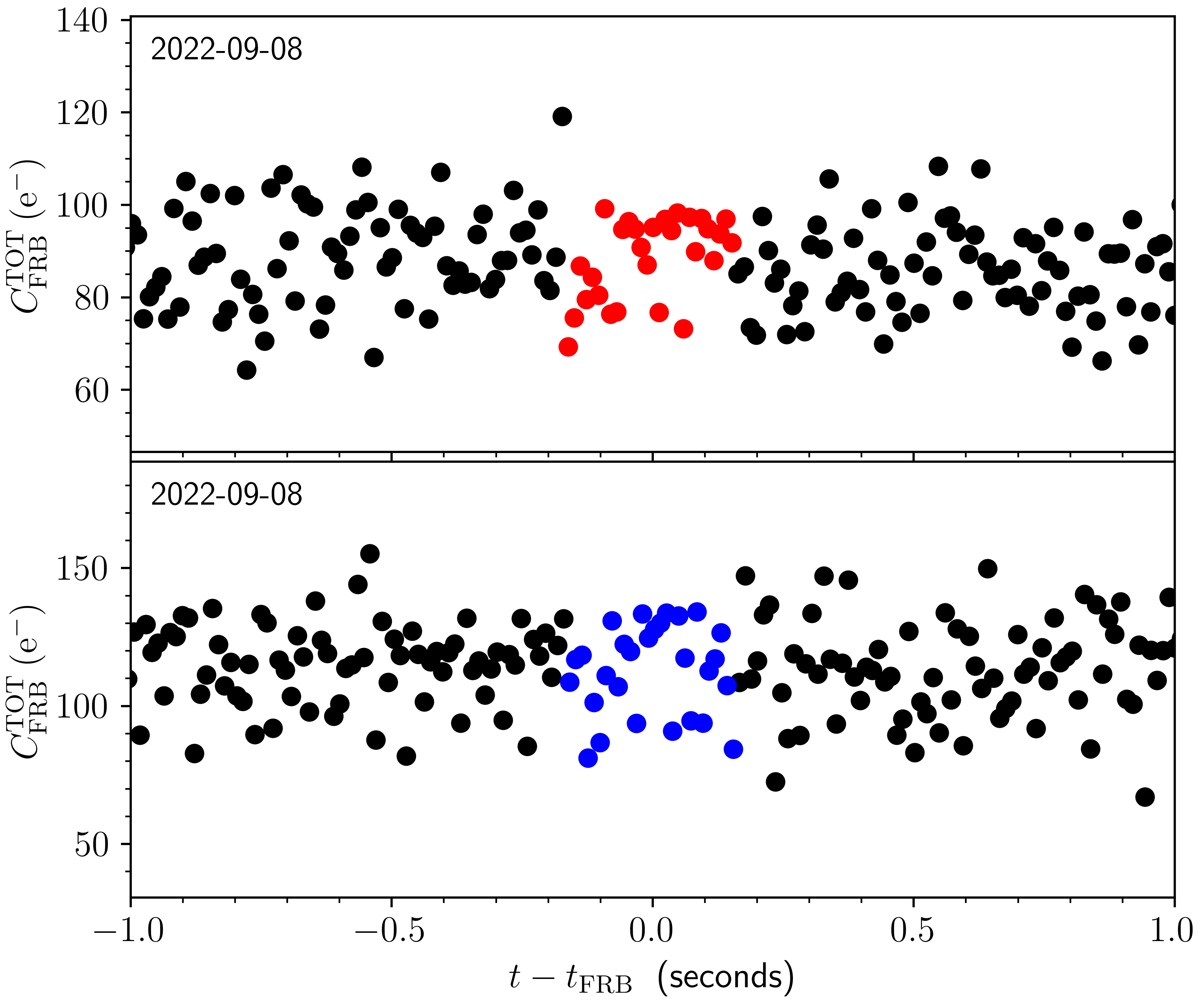
Figure 4: Total counts per exposure in each camera at the FRB location for the $\approx 2$ s around the expected arrival time of optical emission for FRB 20201023 (upper two panels) and FRB 20220908 (lower two panels). The colored dots show the $\Delta t\approx\pm 163$ ms interval corresponding to the absolute timing uncertainty of the ‘Alopeke cameras. There is no evident excess emission for any exposure during these intervals.

Figure 4 shows the subset of count measurements near the predicted arrival time for the optical emission of FRB 20201023 and FRB 20220908. Within the time interval corresponding to the systematic uncertainty of the absolute timing for the ‘Alopeke camera around FRB 20201023 (i.e., $\pm$162 ms from the time calculated in Section 2.4), the red camera recorded 28 measurements with a maximum of ${\rm max}(C_{\rm FRB}^{\rm Tot})=57.8$ ${\rm e^{-}~{}exposure^{-1}}$ or less than $2\sigma$ from the mean count-rate during the full set of observations. Accounting for the multiple measurements within the time interval, the percentage of random draws with one or more measurements having $C_{\rm FRB}^{\rm FRB}>{\rm max}(C_{\rm FRB}^{\rm Tot})$ is 81%. Results for the blue camera are similar with ${\rm max}(C_{\rm FRB}^{\rm Tot})=58.9$ ${\rm e^{-}~{}exposure^{-1}}$. We repeat this analysis for FRB 20220908, finding ${\rm max}(C_{\rm FRB}^{\rm Tot})=99.2$ ${\rm e^{-}~{}exposure^{-1}}$, 1.2$\sigma$ above the mean in the red camera, and ${\rm max}(C_{\rm FRB}^{\rm Tot})=134.2$ ${\rm e^{-}~{}exposure^{-1}}$, 1.3$\sigma$ above the mean in the blue camera. We conclude that any prompt optical emission associated with either radio burst is not detected. Furthermore, we report that we do not see any sources of emission at $>$10$\sigma$ at the site of FRB 20180916B across any of our data sets.

We proceed to estimate a conservative upper limit to the optical fluence of the FRB in both epochs and cameras. We generate Monte Carlo realizations of the experiment by generating mock observed counts at the FRB location during the event:

$$C_{\rm FRB}^{\rm Tot}=C_{\rm FRB}^{\rm other}+C_{\rm FRB}^{\rm FRB}$$ (1)

with $C_{\rm FRB}^{\rm other}$ described by the probability density function (PDF) of counts taken off the event (i.e., background) and $C_{\rm FRB}^{\rm FRB}$ is drawn from a PDF for FRB emission in a single 10.4 ms frame. For the former, we simply adopt the encircled flux throughout each entire observation (i.e., the values shown in Figure 3), which is relatively constant throughout both data sets. For the latter, we assume a Poisson PDF with mean $\mu_{\rm FRB}$ and that the emission is limited to a single exposure. We draw 100 realizations of the $\approx 100,000$ $C_{\rm FRB}^{\rm FRB}$ measurements, increment these by random draws from the Poisson PDF for the FRB, and assess the fraction that exceed ${\rm max}(C_{\rm FRB}^{\rm Tot})$.

Figure 5 shows the results for a range of $\mu_{\rm FRB}$. For FRB 20201023, we find that 99.73% of a random ensemble would exceed ${\rm max}(C_{\rm FRB}^{\rm Tot})$ for (blue camera) $\mu_{\rm FRB}^{99.9}\approx 38.9$ ${\rm e^{-}~{}exposure^{-1}}$ and (red camera) $\mu_{\rm FRB}^{99.9}\approx 51.6$ ${\rm e^{-}~{}exposure^{-1}}$. Similarly, we find that for FRB 20220908, 99.73% of the ensemble would exceed ${\rm max}(C_{\rm FRB}^{\rm Tot})$ for (blue camera) $\mu_{\rm FRB}^{99.9}\approx 76.2$ ${\rm e^{-}~{}exposure^{-1}}$ and (red camera) $\mu_{\rm FRB}^{99.9}\approx 42.0$ ${\rm e^{-}~{}exposure^{-1}}$. In the following, we use these single-exposure count-rate upper limits for constraining the FRB optical emission.

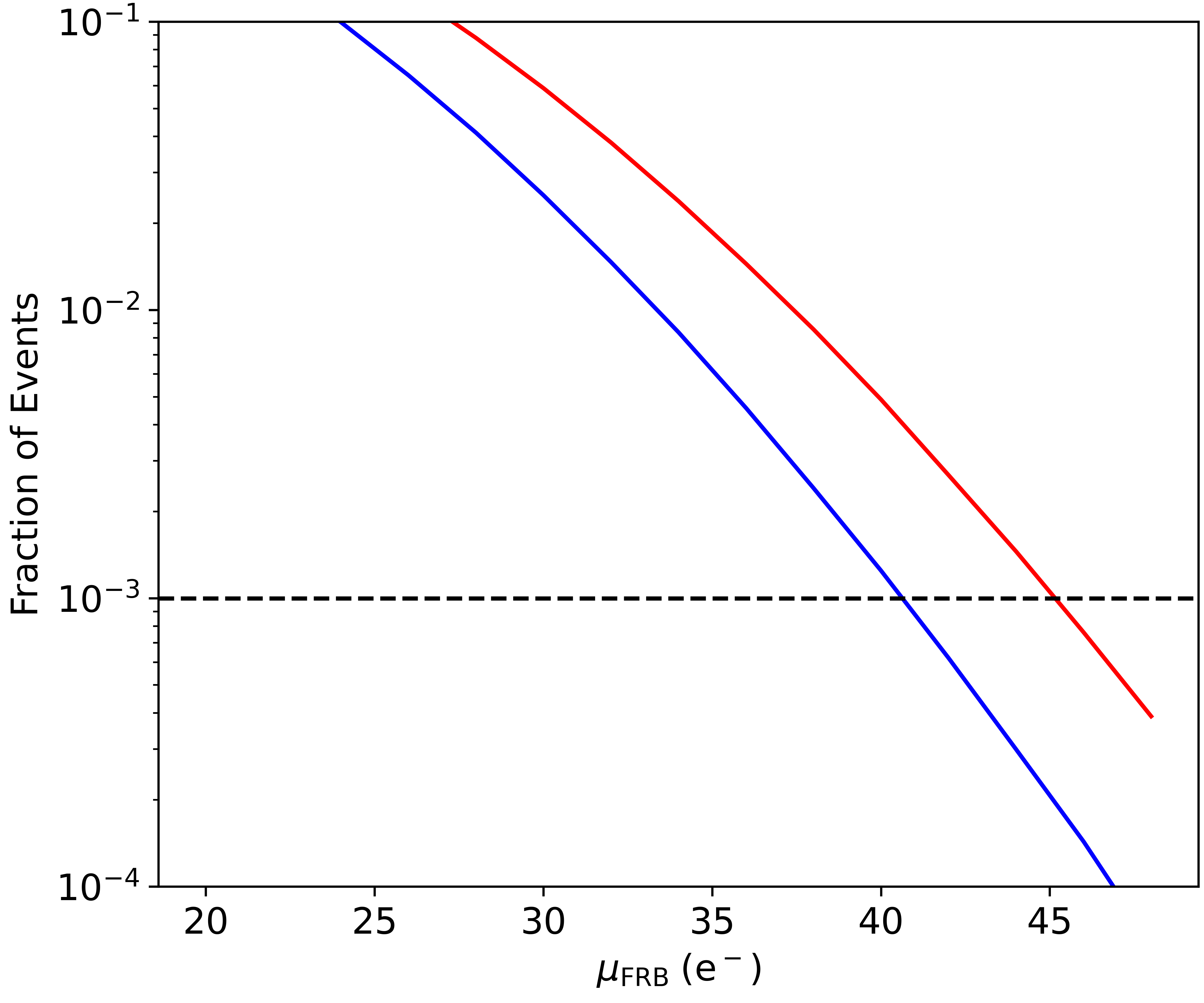
Figure 5: Fraction of simulated events that would not exceed the observed maximum counts ${\rm max}(C_{\rm FRB}^{\rm Tot})$ in the FRB arrival interval as a function of assumed mean counts $\mu_{\rm FRB}$ (Poisson) contributed to a single exposure by the FRB emission. Adopting a confidence level of 99.9% (corresponding to the horizontal dashed line), we set an upper limit of $\mu_{\rm FRB}^{99.9}=38.9\,\rm e^{-}$ (blue line) and $\mu_{\rm FRB}^{99.9}=51.6\,\rm e^{-}$ for the red camera (red line) for FRB 20201023 and $\mu_{\rm FRB}^{99.9}=76.2\,\rm e^{-}$ (blue line) and $\mu_{\rm FRB}^{99.9}=42.0\,\rm e^{-}$ for the red camera (red line) for FRB 20220908.

3.3 Time-variable Sensitivity Function for ‘Alopeke

Key to our optical fluence limits are the photometric accuracy with which we can measure the count rate from Star-1 and Star-2 in each image frame. Figure 3 shows the measured counts in each camera at the FRB location $C_{\rm FRB}^{\rm Tot}$, Star-1, and Star-2 for the full duration of all exposures. In the first radio burst FRB 20201023, the ‘Alopeke data around the optical arrival time show a small gradient in the count-rate for the individual exposures of Star-1 in time that we measure from a linear fit to be $dC_{\rm Star-1}^{\rm Tot}/dt\approx 0.043$ and $\approx 0.015\;{\rm e^{-}\,s^{-1}}$ for the blue and red cameras, respectively, in a 2 minute window around the time of the radio burst. This drift is a small fraction of the average count rate for Star-1 in both cameras during this time interval (see Table 1 and Table 2), implying that the sensitivity function can be approximated from the entire ensemble of data with a source having a flux 1 ${\rm e^{-}~{}exposure^{-1}}$ corresponding to 22.35 AB mag in the red camera and 22.43 AB mag in the blue camera.

However, as shown in the overall count rates of Star-1 and Star-2 from the second burst on 2022-09-08, the flux from Star-1 and Star-2 is significantly variable, especially across the second half of the observation when the radio burst occurred. This effect is correlated across the blue and red detectors and both stars, indicating that it is most likely due to grey opacity due to clouds and thus it affects both detectors simultaneously. We further demonstrate this effect in Figure 6, which presents the individual photometric measurements at the FRB location versus those of Star-1 in units of standard deviation off the mean. The nearly symmetrical distribution during the first observation epoch indicates that the observed fluctuations are uncorrelated, that is the fluctuations in the counts are dominated by random, statistical fluctuations as opposed to systematics (e.g., clouds). However, for the second epoch, there is significant variation toward negative residuals in the flux from Star-1, indicating that the star is frequently obscured by opacity in the atmosphere throughout each exposure.

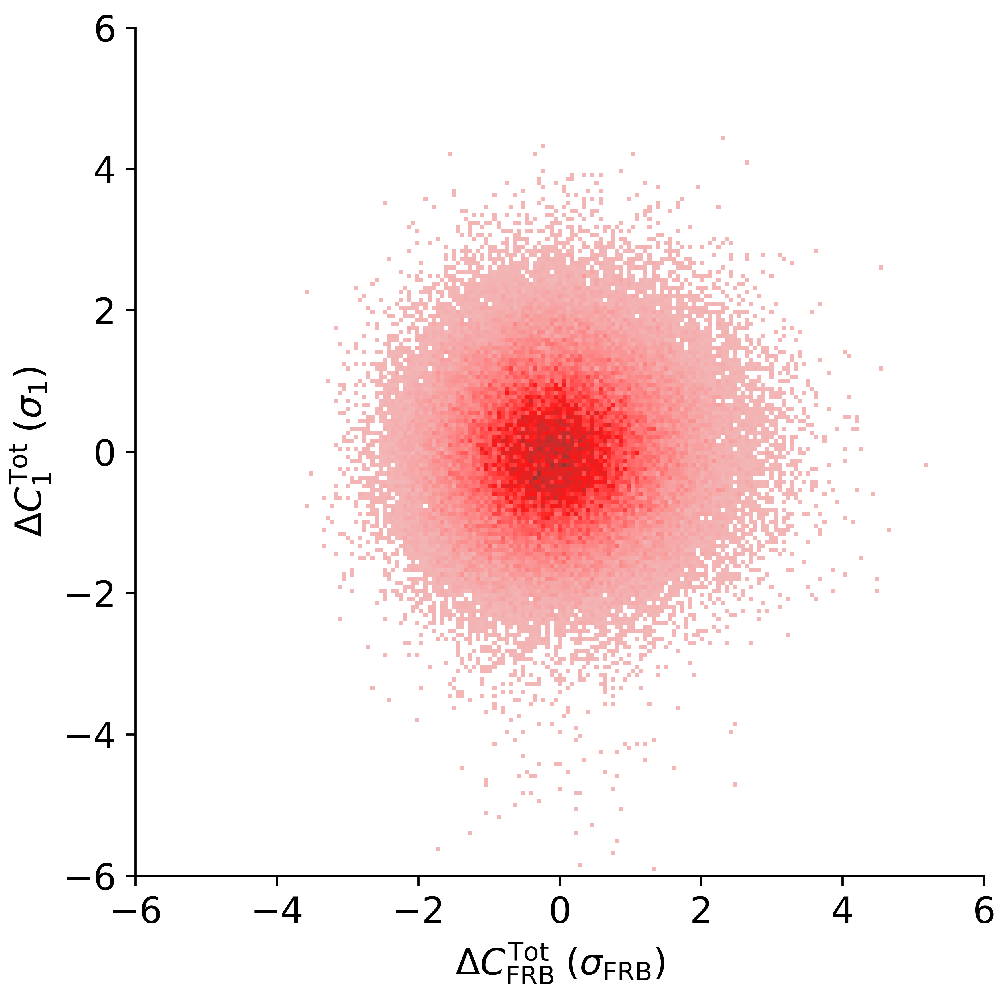
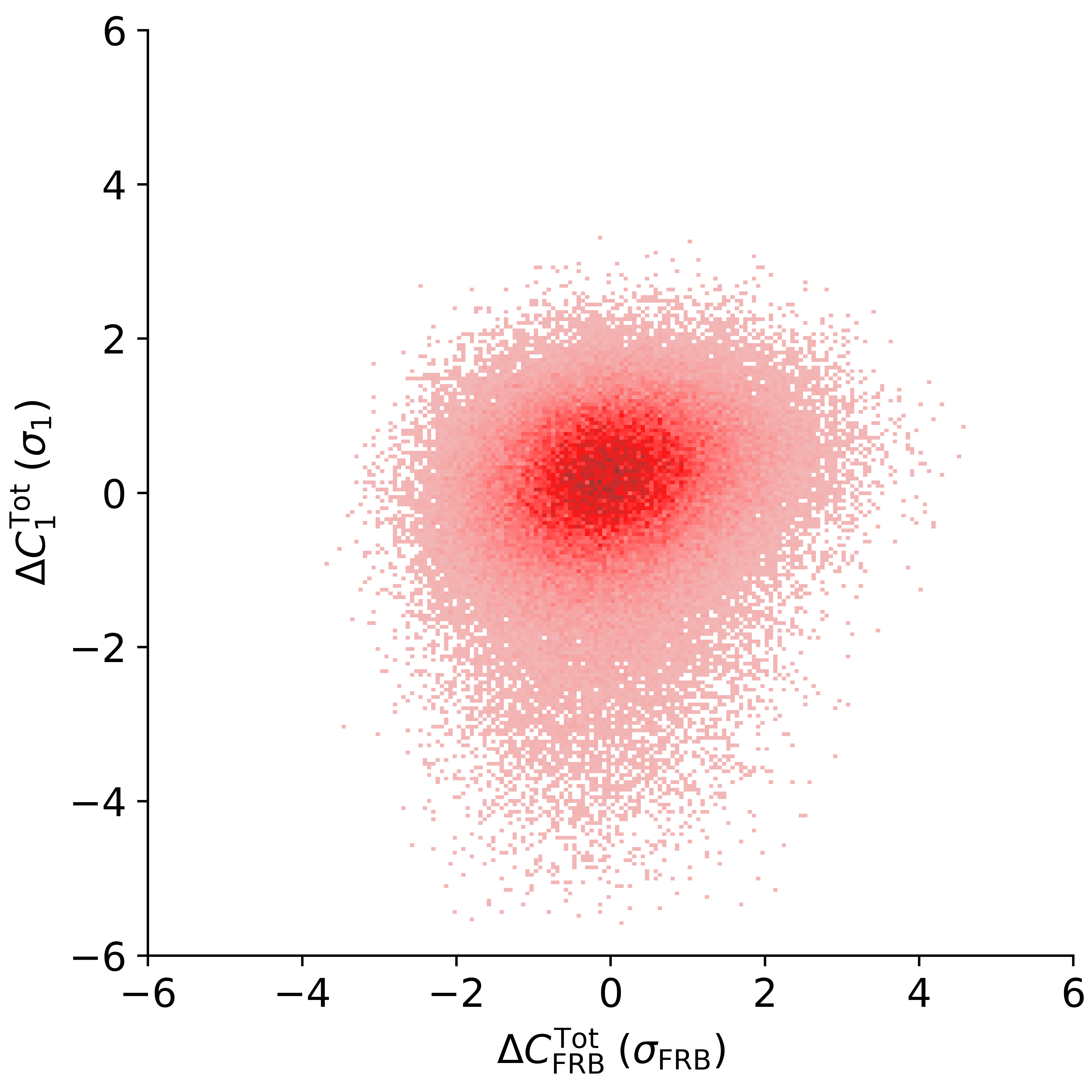
Figure 6: Top panel: Deviations from the mean in units of standard deviation for the ‘Alopeke measurements at the Star-1 against those at the FRB location during the FRB 20201023. The nearly symmetric distribution indicates that the variations in count-rate are dominated by statistical fluctuations. Bottom panel: Same as the top panel but for the ‘Alopeke observations obtained during FRB 20220908. Significant variation from the mean toward negative values for Star-1 indicate that many of these observations were obtained in non-photometric conditions, also seen in Figure 3.

We do not expect these effects to vary significantly within the 163 ms range we consider to derive the count-rate upper limit, therefore we estimate the encircled flux at the FRB position (i.e., in units of $\mu$Jy) by deriving the zero point for every frame from $C_{\rm Star-1}^{\rm Tot}$ and $C_{\rm Star-2}^{\rm Tot}$ compared with their Pan-STARRS $r$ and $i$-band magnitudes. The count rates in Table 1 and Table 2 demonstrate that in both epochs, the count rate varied within expectations for a Poisson distribution. Indeed, for both Star-1 and Star-2, the flux appears higher in the second epoch, implying that the throughput for the Gemini-N/‘Alopeke system was higher at that time and our limits are more constraining in spite of fluctuations in the atmospheric transmission.

Taking the average zero point derived jointly from both stars within the $\pm$163 ms window around each radio burst arrival time, we find that the 99.73% confidence interval count-rate limits in Section 3.2 correspond to $F_{r}<1.38~{}\mu$Jy s and $F_{i}<2.01~{}\mu$Jy s for FRB 20201023 and $F_{r}<3.27~{}\mu$Jy s and $F_{i}<1.84~{}\mu$Jy s for FRB 20220908 before correcting for Milky Way dust and within each 10.4 ms observation. For reference, these limits correspond to a magnitude limit of $m_{r}>18.6$ AB mag and $m_{i}>18.2$ AB mag for FRB 20201023 and $m_{r}>17.7$ AB mag and $m_{i}>18.3$ AB mag for FRB 20220908 also before correcting for Milky Way dust and within each 10.4 ms observation.

After we correct for line-of-sight extinction and at the assumed distance to FRB 20180916B, we estimate the isotropic equivalent specific energy within each band of $E_{\nu}=4\pi D_{L}^{2}f_{\nu}$. Along with the effective frequency of each waveband assuming $\lambda_{\rm eff}$ of 6231 and 7625 Å for $r$- and $i$-bands, respectively, we derive $\nu E_{\nu,r}<1.4\times 10^{41}$ erg and $\nu E_{\nu,i}<8.8\times 10^{40}$ erg for FRB 20201023 and $\nu E_{\nu,r}<3.2\times 10^{41}$ erg and $\nu E_{\nu,i}<8.1\times 10^{40}$ erg for FRB 20220908. We adopt these values for comparing to the radio fluence of each burst and the multi-wavelength energetics of FRB 20180916B in the following discussion.

4 Results and Discussion

Compared with the radio fluence of FRB 20201023 and FRB 20220908 (Section 2.1), our limits correspond to optical-to-radio fluence ratios of $\eta_{\nu}\equiv F_{\rm opt}/F_{\rm radio}<$2–7$\times 10^{-3}$ (note that similar to, e.g., Chen et al., 2020, we use the $\nu$ subscript to distinguish from the ratio of the total energy radiated in each band). Figure 7 shows our fluence ratio limits versus the radio energy and are comparable to the upper end of fluence ratios from optical pulsars, the expected broadband optical counterpart from SGR 1935+2154 (using analysis in De et al., 2020, as described below), and various progenitor models presented in Yang et al. (2019). These are the deepest limits to date for any radio burst on timescales $\lesssim$10 ms, providing useful constraints for the progenitor system and emission model powering the rapid but energetic radio burst. Throughout this section, we analyze these limits in the context of predictions for fast optical burst counterparts to FRBs.

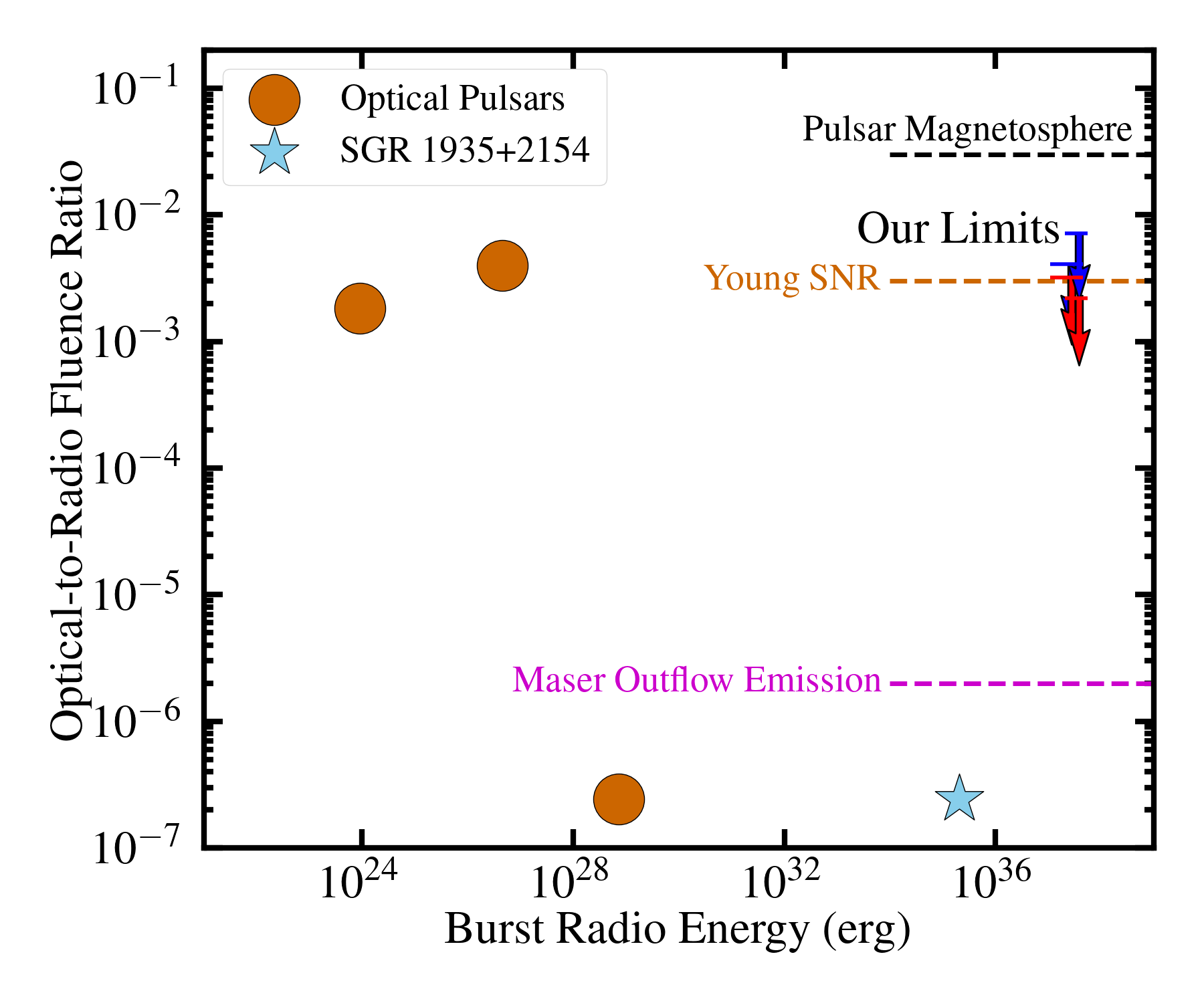
Figure 7: Our limits (downward arrows) on the optical-to-radio fluence ratio from FRB 20180916B in $r$- (blue) and $i$-bands (red). We also compare to the optical-to-radio fluence ratios from the Crab, Geminga, and Vela optical pulsars (Section 4.2) as well as the expected ratio for the bursts from the Galactic magnetar SGR 1935+2154 (Section 4.3). Finally, we also plot the approximate fluence ratios (dashed lines) predicted for various FRB progenitor and emission models from Yang et al. (2019), including inverse Compton emission from a pulsar magnetosphere or young supernova remnant (SNR) as well as synchrotron maser emission from an outflow from a magnetar.

4.1 Constraints on the Optical Energetics

Compared with previous efforts to observe optical emission from FRB 20121102A using ULTRACAM (Hardy et al., 2017), our fluence limits are a factor of 100$\times$ more constraining in the same bandpass and over timescales a factor of $\approx$7$\times$ faster (10.4 ms versus 70.7 ms). Given that FRB 20180916B is $>$6$\times$ closer than FRB 20121102A (which is at a redshift $z=0.193$ or $D_{L}=950$ Mpc; Tendulkar et al., 2017) and has a comparable line-of-sight extinction, our constraints on the energy scale of any optical burst are therefore $\approx$4500$\times$ more constraining. Similar efforts targeting millisecond-timescale optical emission from FRBs have been conducted with the Tomo-e Gozen high-speed CMOS camera observing 11 bursts of FRB 20190520B (Niino et al., 2022) and the photomultiplier SiFAP2 and fast optical cameras Aqueye+ and IFI/Iqueye+ targeting FRB 20180916B (Pilia et al., 2020). These observations resulted in energy limits in a wide passband $T$ (370–730 nm) of $\nu E_{\nu,T}=2.9\times 10^{43}$ erg on FRB 20190520B on a timescale of 40.9 ms and in $V$-band on $\nu E_{\nu,V}=1.5\times 10^{41}$ erg on a timescale of 1 ms for FRB 20180916B. Our limits on energy are significantly more constraining on similar timescales, yielding the best constraints to date on millisecond timescale optical emission contemporaneous with a FRB.

4.2 Comparison to Optical Emission from Pulsars

Pulsars observed in the Milky Way galaxy are among the closest analogs to extragalactic FRBs that also have optical detections simultaneous with their radio bursts, with seven such known “optical pulsars” (Cocke et al., 1969; Peterson et al., 1978; Middleditch et al., 1987; Shearer et al., 1997, 1998; Kern et al., 2003; Słowikowska et al., 2009; Ambrosino et al., 2017). The best-studied example is the Crab pulsar (see Bühler & Blandford, 2014, for a review), which exhibits radio pulses known to correlate with enhanced optical pulse emission (Shearer et al., 2003), a progenitor model that has been extrapolated up to higher burst energies for some FRBs (Lyutikov et al., 2016). The optical pulses are characteristically wider in time than the radio pulses roughly by a factor of 5, with the peak of the emission arriving before that of the radio pulse.

These pulses can exhibit a range of optical fluence ratios, but on average are measured to have $\eta_{\nu}\approx 10^{-3}$ (Bühler & Blandford, 2014, see their phase-averaged emission in Fig. 2). We show them for comparison in Figure 7 as orange circles. Note that this quantity depends sensitively on the choice of radio band used in normalizing the fluence ratio due to the steep spectral indices of Crab pulses from $\nu^{-2.2}$ to $\nu^{-4.9}$ (Karuppusamy et al., 2010). Here we choose the spectrum of the Crab pulsar at 400 MHz from Bühler & Blandford (2014) for direct comparison to the CHIME radio fluence from FRB 20180916B and assume an average radio burst duration of 300 $\mu$s (consistent with Shearer et al., 2003) in deriving the emitted radio energy per pulse. We also compared to the emitted radio energy from the Geminga and Vela pulsars (also shown as orange circles in Figure 7), whose phase-averaged spectral energy distributions are presented in Danilenko et al. (2011) for Geminga and Mignani et al. (2017) for Vela. For the former, we assume a 400 MHz brightness of 100 $\mu$Jy, and exhibit a large range in optical-to-radio fluence ratios from $\sim 2\times 10^{-3}$ to $2\times 10^{-7}$ for Geminga and Vela, respectively.

While it is informative to investigate the ratio of radiated optical energy on short timescales for bursts from other neutron stars, we note that our limits require a moderately lower optical energy than the Crab and Geminga pulsars. It will be challenging to rule out optical bursts with total fluences four orders of magnitude less energetic than our limits and similar to Vela without a burst closer than a few Mpc whose emitted radio energy is comparable to FRB 20180916B. We therefore turn to other sources and emission models more directly comparable to FRB 20180916B and theoretically capable of partitioning a much larger fraction of energy into optical emission.

4.3 Comparison to Galactic Magnetar SGR 1935+2154

Another potential local analog to FRB progenitors is the Galactic magnetar SGR 1935+2154, from which FRB-like pulses have been observed (Bochenek et al., 2020b; CHIME/FRB Collaboration et al., 2020). Located in Galactic center, it is severely affected by dust extinction and thus despite some efforts to observe their putative optical and infrared counterparts, these have been unsuccessful (e.g., De et al., 2020; Zampieri et al., 2022; Hiramatsu et al., 2022). However, some of these radio pulses have presented simultaneous X-rays emission (Mereghetti et al., 2020; Ridnaia et al., 2021; Tavani et al., 2021).

Using the simultaneous X-ray and radio detection of this source, we adopt the analysis in De et al. (2020) to interpolate the expected optical-to-radio fluence ratio. Here we assume a continuous, broadband power law between the radio and hard X-ray detections of STARE2 (Bochenek et al., 2020a) and its X-ray counterpart as observed by Konus-Wind (Ridnaia et al., 2021). Such a spectrum would be expected if the emission in both wavebands is dominated by a synchrotron spectrum with a peak energy at higher energies than the hard X-ray band at 18–320 keV, which is predicted by some emission models such as the synchrotron maser (Metzger et al., 2019; Margalit et al., 2020). Under this assumption and the $F_{\nu}\sim\nu^{-0.46}$ spectrum predicted in De et al. (2020), we predict that the optical fluence ratio between 400 MHz and $i$-band would be $\sim 3\times 10^{-3}$, very close to what we predict for the Crab pulsar (Figure 7). Our limits can rule out such a counterpart, albeit for bursts than moderately higher radio energies (factor of $>$1000) that obtain with FRB 20180916B.

4.4 Implications for Progenitor and Emission Models

Finally, we compare our limits on optical counterparts to progenitor and emission models presented in Yang et al. (2019), which are shown as dashed lines in Figure 7. Specifically, these models correspond to emission from a pulsar magnetosphere and from a young supernova remnant (SNR), which we can rule out, as well as maser emission in an outflow from a young magnetar, which we are not able to rule out with our limits. The first model (see Kumar et al., 2017; Yang & Zhang, 2018) produces optical emission from energetic electrons in the magnetosphere of a pulsar, which scatter radio emission to optical wavelengths and primarily depends on the magnetic field strength and rotation rate of the young pulsar. The former is expected to be extremely high for FRB progenitor systems (e.g., SGR 1935+2154 is $\approx$2.2$\times$10¹⁴ G; Israel et al., 2016), though the rotation period is uncertain. For the upper range of expected fluence ratios in Yang et al. (2019) (see, e.g., their Fig. 3) we can rule out such an emission mechanism.

The second emission model corresponds to inverse Compton emission from the energetic electrons in a young supernova remnant or pulsar wind nebula (e.g., Piro, 2016). Here the density and total energy of the electron population depends on the age, ejecta mass, and total energy of the initial explosion. Again, we can rule out the most massive, youngest, and low energy explosions based on the range of expected values presented in Yang et al. (2019). However, this progenitor model is complicated by the fact that extremely young SNRs would obscure the underlying FRB with free-free opacity, as well as the fact that modern time-domain surveys (e.g., Bellm et al., 2019; Jones et al., 2021) place deep limits on the presence of a typical supernova on the timescales explored by Yang et al. (2019).

We also considered maser emission from an inverted population of electrons in an outflow or burst of ejecta around a young magnetar. This model has been explored in detail in the literature (Lyubarsky, 2014; Beloborodov, 2017; Waxman, 2017; Lu & Kumar, 2018; Metzger et al., 2019; Margalit et al., 2020). It is a promising model for optical counterparts because some emission mechanisms predict a longer-lived afterglow that can in principle be detected by untargeted surveys such as the Vera C. Rubin Observatory’s Legacy Survey of Space and Time (Yang et al., 2019) or targeted follow up of FRBs (Kilpatrick et al., 2021; Hiramatsu et al., 2022; Trudu et al., 2023). Given the timescale of our observations, we consider a prompt optical counterpart with a millisecond timescale, which in general will have a fluence $\approx 2\times 10^{-6}$ that of the radio (Yang et al., 2019). Our limits do not approach this level, leaving room for future exploration of intrinsically more energetic bursts or those much closer than FRB 20180916B.

4.5 Prospects for Additional High-speed Follow up of FRBs

Given its status as one of the earliest discovered repeating FRBs, proximity at 150 Mpc, and especially its periodicity, FRB 20180916B has been a prime target in the search for multi-wavelength emission from FRBs (Andreoni et al., 2020; Pilia et al., 2020; Kilpatrick et al., 2021; Trudu et al., 2023). However, the lack of detections at all frequencies a few GHz despite these concerted efforts has placed strong constraints on multi-wavelength emission counterparts and the emission mechanisms described above. It remains open whether FRB 20180916B is representative of the known FRB population or if there can be multiple progenitor and emission channels with a variety of optical-to-radio fluence ratios.

Hiramatsu et al. (2022) found that targeted follow up within 3 days of a new burst from a repeating FRB yielded observations coincident with a subsequent burst $\approx$40% of the time. As opposed to our strategy of targeting the periodic FRB 20180916B near the peak of its expected activity period, this strategy possible new optical burst detections across a variety of sources and deeper luminosity limits for those at closer distances (e.g., the repeating FRB in a globular cluster of M81 at 3.6 Mpc, FRB 20200120E; Kirsten et al., 2022). At the same time, untargeted follow up from optical surveys will be extremely valuable both for prompt counterpart detections (Yang et al., 2019) as well as pre-burst and post-burst constraints on supernova emission or more exotic optical counterparts (e.g., the stellar merger counterpart in Sridhar et al., 2021). Continued optical follow up will therefore play an important role in determining the FRB mechanism and its progenitor source.

5 Conclusions

We have presented high-speed ($\approx 10$ ms) optical follow up of FRB 20180916B with the ‘Alopeke camera at Gemini-North observatory contemporaneous with two radio bursts, FRB 20201023 and FRB 20220908, detected by the CHIME array. In summary, we find:

1. There are no prompt optical counterparts in our data after correcting for the effects of dispersion, light-travel time, and the uncertainties in the internal clocks between ‘Alopeke and CHIME. Accounting for these uncertainties, we derive limits on optical fluence in each of the 10.4 ms time bins of our ‘Alopeke data in $r$- and $i$-bands of $<$1.38–3.27 $\mu$Jy s, corresponding to a total emitted optical energy of $<$8.1–32.0$\times$10⁴⁰ erg and optical-to-radio (400 MHz) fluence ratios of 2–7$\times$10^-3.

2. Comparing to expectations for optical pulsars or the broadband optical emission from the Galactic magnetar SGR 1935+2154, we rule out sources with the largest partition of optical-to-radio energies, which in general are around $3\times 10^{-3}$. However, there is a large range in values for these sources, such as the Vela pulsar with $2\times 10^{-7}$, and limits on optical counterparts from such a source would only be possible for the closest or most energetic FRBs.

3. We also compare to expected models of FRBs and are able to rule out several types of inverse Compton emission presented in Yang et al. (2019), for example from a pulsar magnetosphere or supernova remnant, but not for the lowest energy inverse Compton counterparts or a synchrotron maser.

Data and Software Availability

All data and analysis products presented in this article are available upon request. Analysis code and photometry used in this paper are available at https://github.com/profxj/papers/tree/master/FRB/Alopeke. The Gemini data are publicly available on the Gemini data archive at https://archive.gemini.edu/.

References

- Ambrosino et al. (2017) Ambrosino, F., Papitto, A., Stella, L., et al. 2017, Nature Astronomy, 1, 854, doi: 10.1038/s41550-017-0266-2
- Andreoni et al. (2020) Andreoni, I., Lu, W., Smith, R. M., et al. 2020, ApJ, 896, L2, doi: 10.3847/2041-8213/ab94a5
- Bellm et al. (2019) Bellm, E. C., Kulkarni, S. R., Graham, M. J., et al. 2019, PASP, 131, 018002, doi: 10.1088/1538-3873/aaecbe
- Beloborodov (2017) Beloborodov, A. M. 2017, ApJ, 843, L26, doi: 10.3847/2041-8213/aa78f3
- Bhandari et al. (2020) Bhandari, S., Sadler, E. M., Prochaska, J. X., et al. 2020, ApJ, 895, L37, doi: 10.3847/2041-8213/ab672e
- Bochenek et al. (2020a) Bochenek, C., Kulkarni, S., Ravi, V., et al. 2020a, The Astronomer’s Telegram, 13684, 1
- Bochenek et al. (2020b) Bochenek, C. D., Ravi, V., Belov, K. V., et al. 2020b, arXiv e-prints, arXiv:2005.10828. https://arxiv.org/abs/2005.10828
- Bradley et al. (2022) Bradley, L., Sipőcz, B., Robitaille, T., et al. 2022, astropy/photutils: 1.6.0, 1.6.0, Zenodo, Zenodo, doi: 10.5281/zenodo.7419741
- Bradley et al. (2023) —. 2023, astropy/photutils: 1.9.0, 1.9.0, Zenodo, Zenodo, doi: 10.5281/zenodo.8248020
- Bühler & Blandford (2014) Bühler, R., & Blandford, R. 2014, Reports on Progress in Physics, 77, 066901, doi: 10.1088/0034-4885/77/6/066901
- Chambers et al. (2016a) Chambers, K. C., Magnier, E. A., Metcalfe, N., et al. 2016a, arXiv e-prints, arXiv:1612.05560. https://arxiv.org/abs/1612.05560
- Chambers et al. (2016b) —. 2016b, arXiv e-prints, arXiv:1612.05560. https://arxiv.org/abs/1612.05560
- Chen et al. (2020) Chen, G., Ravi, V., & Lu, W. 2020, ApJ, 897, 146, doi: 10.3847/1538-4357/ab982b
- CHIME/FRB Collaboration et al. (2018) CHIME/FRB Collaboration, Amiri, M., Bandura, K., et al. 2018, ApJ, 863, 48, doi: 10.3847/1538-4357/aad188
- CHIME/FRB Collaboration et al. (2019) CHIME/FRB Collaboration, Andersen, B. C., Bandura, K., et al. 2019, ApJ, 885, L24, doi: 10.3847/2041-8213/ab4a80
- CHIME/FRB Collaboration et al. (2020) CHIME/FRB Collaboration, Andersen, B. C., Bandura, K. M., et al. 2020, Nature, 587, 54, doi: 10.1038/s41586-020-2863-y
- Chime/Frb Collaboration et al. (2020) Chime/Frb Collaboration, Amiri, M., Andersen, B. C., et al. 2020, Nature, 582, 351, doi: 10.1038/s41586-020-2398-2
- CHIME/FRB Collaboration et al. (2021) CHIME/FRB Collaboration, Amiri, M., Andersen, B. C., et al. 2021, ApJS, 257, 59, doi: 10.3847/1538-4365/ac33ab
- Cocke et al. (1969) Cocke, W. J., Disney, M. J., & Taylor, D. J. 1969, Nature, 221, 525, doi: 10.1038/221525a0
- Cordes & Chatterjee (2019) Cordes, J. M., & Chatterjee, S. 2019, ARA&A, 57, 417, doi: 10.1146/annurev-astro-091918-104501
- Danilenko et al. (2011) Danilenko, A. A., Zyuzin, D. A., Shibanov, Y. A., & Zharikov, S. V. 2011, MNRAS, 415, 867, doi: 10.1111/j.1365-2966.2011.18753.x
- Day et al. (2020) Day, C. K., Deller, A. T., Shannon, R. M., et al. 2020, MNRAS, 497, 3335, doi: 10.1093/mnras/staa2138
- De et al. (2020) De, K., Ashley, M. C. B., Andreoni, I., et al. 2020, ApJ, 901, L7, doi: 10.3847/2041-8213/abb3c5
- Flewelling et al. (2020) Flewelling, H. A., Magnier, E. A., Chambers, K. C., et al. 2020, ApJS, 251, 7, doi: 10.3847/1538-4365/abb82d
- Fong et al. (2021) Fong, W.-f., Dong, Y., Leja, J., et al. 2021, ApJ, 919, L23, doi: 10.3847/2041-8213/ac242b
- Fonseca et al. (2020) Fonseca, E., Andersen, B. C., Bhardwaj, M., et al. 2020, ApJ, 891, L6, doi: 10.3847/2041-8213/ab7208
- Fonseca et al. (2023) Fonseca, E., Pleunis, Z., Breitman, D., et al. 2023, arXiv e-prints, arXiv:2311.05829. https://arxiv.org/abs/2311.05829
- Gaia Collaboration et al. (2018) Gaia Collaboration, Brown, A. G. A., Vallenari, A., et al. 2018, A&A, 616, A1, doi: 10.1051/0004-6361/201833051
- Ghisellini & Locatelli (2018) Ghisellini, G., & Locatelli, N. 2018, A&A, 613, A61, doi: 10.1051/0004-6361/201731820
- Gordon et al. (2023) Gordon, A. C., Fong, W.-f., Kilpatrick, C. D., et al. 2023, arXiv e-prints, arXiv:2302.05465, doi: 10.48550/arXiv.2302.05465
- Hardy et al. (2017) Hardy, L. K., Dhillon, V. S., Spitler, L. G., et al. 2017, MNRAS, 472, 2800, doi: 10.1093/mnras/stx2153
- Heintz et al. (2020) Heintz, K. E., Prochaska, J. X., Simha, S., et al. 2020, ApJ, 903, 152, doi: 10.3847/1538-4357/abb6fb
- Hiramatsu et al. (2022) Hiramatsu, D., Berger, E., Metzger, B. D., et al. 2022, arXiv e-prints, arXiv:2211.03974, doi: 10.48550/arXiv.2211.03974
- Israel et al. (2016) Israel, G. L., Esposito, P., Rea, N., et al. 2016, MNRAS, 457, 3448, doi: 10.1093/mnras/stw008
- Ivezić et al. (2019) Ivezić, Ž., Kahn, S. M., Tyson, J. A., et al. 2019, ApJ, 873, 111, doi: 10.3847/1538-4357/ab042c
- Jones et al. (2021) Jones, D. O., Foley, R. J., Narayan, G., et al. 2021, ApJ, 908, 143, doi: 10.3847/1538-4357/abd7f5
- Karpov et al. (2019) Karpov, S., Jelinek, M., & Štrobl, J. 2019, Astronomische Nachrichten, 340, 613, doi: 10.1002/asna.201913664
- Karuppusamy et al. (2010) Karuppusamy, R., Stappers, B. W., & van Straten, W. 2010, A&A, 515, A36, doi: 10.1051/0004-6361/200913729
- Katz (2018) Katz, J. I. 2018, MNRAS, 481, 2946, doi: 10.1093/mnras/sty2459
- Kern et al. (2003) Kern, B., Martin, C., Mazin, B., & Halpern, J. P. 2003, ApJ, 597, 1049, doi: 10.1086/378670
- Kilpatrick et al. (2021) Kilpatrick, C. D., Burchett, J. N., Jones, D. O., et al. 2021, ApJ, 907, L3, doi: 10.3847/2041-8213/abd560
- Kirsten et al. (2022) Kirsten, F., Marcote, B., Nimmo, K., et al. 2022, Nature, 602, 585, doi: 10.1038/s41586-021-04354-w
- Kumar et al. (2017) Kumar, P., Lu, W., & Bhattacharya, M. 2017, MNRAS, 468, 2726, doi: 10.1093/mnras/stx665
- Lindegren et al. (2018) Lindegren, L., Hernández, J., Bombrun, A., et al. 2018, A&A, 616, A2, doi: 10.1051/0004-6361/201832727
- Lorimer et al. (2007) Lorimer, D. R., Bailes, M., McLaughlin, M. A., Narkevic, D. J., & Crawford, F. 2007, Science, 318, 777, doi: 10.1126/science.1147532
- Lu & Kumar (2018) Lu, W., & Kumar, P. 2018, MNRAS, 477, 2470, doi: 10.1093/mnras/sty716
- Lyubarsky (2014) Lyubarsky, Y. 2014, MNRAS, 442, L9, doi: 10.1093/mnrasl/slu046
- Lyutikov et al. (2016) Lyutikov, M., Burzawa, L., & Popov, S. B. 2016, MNRAS, 462, 941, doi: 10.1093/mnras/stw1669
- MAGIC Collaboration et al. (2018) MAGIC Collaboration, Acciari, V. A., Ansoldi, S., et al. 2018, MNRAS, 481, 2479, doi: 10.1093/mnras/sty2422
- Marcote et al. (2020) Marcote, B., Nimmo, K., Hessels, J. W. T., et al. 2020, Nature, 577, 190, doi: 10.1038/s41586-019-1866-z
- Margalit et al. (2020) Margalit, B., Beniamini, P., Sridhar, N., & Metzger, B. D. 2020, ApJ, 899, L27, doi: 10.3847/2041-8213/abac57
- Marnoch et al. (2020) Marnoch, L., Ryder, S. D., Bannister, K. W., et al. 2020, A&A, 639, A119, doi: 10.1051/0004-6361/202038076
- Megias Homar et al. (2023) Megias Homar, G., Meyers, J. E., & Kahn, S. M. 2023, arXiv e-prints, arXiv:2303.02525, doi: 10.48550/arXiv.2303.02525
- Mereghetti et al. (2020) Mereghetti, S., Savchenko, V., Ferrigno, C., et al. 2020, ApJ, 898, L29, doi: 10.3847/2041-8213/aba2cf
- Metzger et al. (2019) Metzger, B. D., Margalit, B., & Sironi, L. 2019, MNRAS, 485, 4091, doi: 10.1093/mnras/stz700
- Middleditch et al. (1987) Middleditch, J., Pennypacker, C. R., & Burns, M. S. 1987, ApJ, 315, 142, doi: 10.1086/165119
- Mignani et al. (2017) Mignani, R. P., Paladino, R., Rudak, B., et al. 2017, ApJ, 851, L10, doi: 10.3847/2041-8213/aa9c3e
- Niino et al. (2022) Niino, Y., Doi, M., Sako, S., et al. 2022, ApJ, 931, 109, doi: 10.3847/1538-4357/ac6be8
- Peterson et al. (1978) Peterson, B. A., Murdin, P., Wallace, P., et al. 1978, Nature, 276, 475, doi: 10.1038/276475a0
- Petroff et al. (2022) Petroff, E., Hessels, J. W. T., & Lorimer, D. R. 2022, A&A Rev., 30, 2, doi: 10.1007/s00159-022-00139-w
- Pilia et al. (2020) Pilia, M., Burgay, M., Possenti, A., et al. 2020, ApJ, 896, L40, doi: 10.3847/2041-8213/ab96c0
- Piro (2016) Piro, A. L. 2016, ApJ, 824, L32, doi: 10.3847/2041-8205/824/2/L32
- Piro et al. (2021) Piro, L., Bruni, G., Troja, E., et al. 2021, A&A, 656, L15, doi: 10.1051/0004-6361/202141903
- Rajwade et al. (2020) Rajwade, K. M., Mickaliger, M. B., Stappers, B. W., et al. 2020, MNRAS, 495, 3551, doi: 10.1093/mnras/staa1237
- Ravi et al. (2022) Ravi, V., Law, C. J., Li, D., et al. 2022, MNRAS, 513, 982, doi: 10.1093/mnras/stac465
- Ridnaia et al. (2021) Ridnaia, A., Svinkin, D., Frederiks, D., et al. 2021, Nature Astronomy, 5, 372, doi: 10.1038/s41550-020-01265-0
- Schlafly & Finkbeiner (2011) Schlafly, E. F., & Finkbeiner, D. P. 2011, ApJ, 737, 103, doi: 10.1088/0004-637X/737/2/103
- Scott & Howell (2018) Scott, N. J., & Howell, S. B. 2018, NESSI and ’Alopeke: two new dual-channel speckle imaging instruments, doi: 10.1117/12.2311539
- Scott et al. (2021) Scott, N. J., Howell, S. B., Gnilka, C. L., et al. 2021, Frontiers in Astronomy and Space Sciences, 8, 138, doi: 10.3389/fspas.2021.716560
- Shearer et al. (2003) Shearer, A., Stappers, B., O’Connor, P., et al. 2003, Science, 301, 493, doi: 10.1126/science.1084919
- Shearer et al. (1997) Shearer, A., Redfern, R. M., Gorman, G., et al. 1997, ApJ, 487, L181, doi: 10.1086/310888
- Shearer et al. (1998) Shearer, A., Golden, A., Harfst, S., et al. 1998, A&A, 335, L21, doi: 10.48550/arXiv.astro-ph/9802225
- Słowikowska et al. (2009) Słowikowska, A., Kanbach, G., Kramer, M., & Stefanescu, A. 2009, MNRAS, 397, 103, doi: 10.1111/j.1365-2966.2009.14935.x
- Sridhar et al. (2021) Sridhar, N., Metzger, B. D., Beniamini, P., et al. 2021, ApJ, 917, 13, doi: 10.3847/1538-4357/ac0140
- Tavani et al. (2021) Tavani, M., Casentini, C., Ursi, A., et al. 2021, Nature Astronomy, 5, 401, doi: 10.1038/s41550-020-01276-x
- Tendulkar et al. (2017) Tendulkar, S. P., Bassa, C. G., Cordes, J. M., et al. 2017, ApJ, 834, L7, doi: 10.3847/2041-8213/834/2/L7
- Trudu et al. (2023) Trudu, M., Pilia, M., Nicastro, L., et al. 2023, A&A, 676, A17, doi: 10.1051/0004-6361/202245303
- Waxman (2017) Waxman, E. 2017, ApJ, 842, 34, doi: 10.3847/1538-4357/aa713e
- Yang & Zhang (2018) Yang, Y.-P., & Zhang, B. 2018, ApJ, 868, 31, doi: 10.3847/1538-4357/aae685
- Yang et al. (2019) Yang, Y.-P., Zhang, B., & Wei, J.-Y. 2019, ApJ, 878, 89, doi: 10.3847/1538-4357/ab1fe2
- Zampieri et al. (2022) Zampieri, L., Mereghetti, S., Turolla, R., et al. 2022, ApJ, 925, L16, doi: 10.3847/2041-8213/ac4b60
- Zhang (2020) Zhang, B. 2020, Nature, 587, 45, doi: 10.1038/s41586-020-2828-1
- Zhang (2022) —. 2022, ApJ, 925, 53, doi: 10.3847/1538-4357/ac3979