Bounds on Quartic Gauge Couplings in HEFT from Electroweak Gauge Boson Pair Production at the LHC

Abstract

Precision measurements of anomalous quartic couplings of electroweak gauge bosons allow us to search for deviations of the Standard Model predictions and signals of new physics. Here, we obtain the constraints on anomalous quartic gauge couplings using the presently available data on the production of gauge-boson pairs via vector boson fusion. We work in the Higgs effective theory framework and obtain the present bounds on the operator’s Wilson coefficients. Anomalous quartic gauge boson couplings lead to rapidly growing cross sections and we discuss the impact of a unitarization procedure on the attainable limits.

I Introduction

The Standard Model (SM) $SU(2)_{L}\otimes U(1)_{Y}$ gauge symmetry determines univocally the structure and strength of the triple and quartic couplings among electroweak gauge-bosons. Therefore, measuring independently the triple gauge-boson couplings (TGC) and the quartic gauge-boson couplings (QGC) tests the SM and provides sensitivity to new physics. In a model independent approach, departures from the SM predictions for TGC and QGC can be parametrized by higher-order operators encoding indirect effects of heavy new physics. Furthermore, the analysis of the gauge boson self interactions can probe whether the gauge symmetry is realized linearly or nonlinearly in the low energy effective theory (EFT) of the electroweak symmetry breaking sector [1, 2].

In collider experiments, the pair production of electroweak gauge bosons allows the direct study of TGC [3, 4, 5], while QGC can be probed via the production of three electroweak vector bosons [6, 7, 8, 9, 10, 11, 12], the exclusive production of gauge-boson pairs  [13, 14, 15], or the vector-boson-scattering production of electroweak vector boson pairs [16, 8, 17, 18, 19, 20, 21, 22, 23, 24, 25, 26]. In the EFT approach, the Wilson coefficients of effective operators that contain both TGC and QGC are more strongly constrained through the study of their TGC component.

In order to mitigate the bounds on QGC originating from the TGC analyses, we focus on the so-called genuine QGC operators, that is, effective operators generating QGC but that do not generate any TGC; for models leading to such operators see [27], for instance. The set of operators to be considered depends on the assumed realization of the SM gauge theory in the low-energy EFT in which the nature of the Higgs-like state observed at the LHC in 2012 [28, 29] plays a pivotal role. If the Higgs belongs to a $SU(2)_{L}$ doublet, the SM gauge symmetry can be realized linearly in the effective theory, which, in this case, is usually referred to as standard model effective field theory (SMEFT). In this scenario, the lowest-order genuine QGC are given by dimension-eight operators [30]. Alternatively, if the Higgs boson is a $SU(2)_{L}$ isosinglet, we are lead to use a nonlinear realization of the gauge symmetry and the low energy EFT obtained this way is called Higgs effective theory (HEFT). In this case, the lowest-order QGC appear at ${\cal O}(p^{4})$ [31, 32].

There is one important difference between the QGC generated gauge-linear dimension-eight operators and those generated nonlinearly at ${\cal O}(p^{4})$: in the second case the QGC’s do not involve photons. This fact renders these operators more difficult to observe, specially in the production of three gauge bosons. Consequently, most of the experimental searches have casted their results on QGC as bounds on Wilson coefficients of dimension-eight gauge-linear operators. Furthermore, most experimental searches consider only one Wilson coefficient different from zero at a time. This implies that the results of the experimental searches constraining dimension-eight SMEFT operators, even those which do not involve photons nor derivatives, cannot be directly translated into bounds on the ${\cal O}(p^{4})$ HEFT operators because the last ones are equivalent to combinations of several coefficients of the corresponding dimension-eight SMEFT siblings; see next section for details.

With this motivation, in this work we perform a dedicated combined analysis of searches for genuine QGC in the framework of the ${\cal O}(p^{4})$ HEFT operators. We briefly present in Sec. II the basics of the analysis framework. We focus on the most sensitive channels for the generated QGC which are those with electroweak gauge boson pairs produced in association with two jets, which are dominated by vector boson fusion. Section. III describes the data sets considered and the details of our analysis, while we present our results and their discussion in Section IV.

II Analysis Framework

In this work we consider a dynamical scenario in which the Higgs boson is a pseudo-Nambu-Goldstone boson of a broken global symmetry while being an isosinglet of the SM gauge symmetries. In this case, the gauge symmetry of the low energy effective Lagrangian is realized nonlinearly with a global $SU(2)_{L}\otimes SU(2)_{R}$ symmetry broken to the diagonal $SU(2)_{C}$ [33, 34, 35, 36]. This EFT is a derivative expansion and it is written in terms of the SM fermions and gauge bosons and of the physical Higgs $h$ [1, 31]. The building block at low energies is a dimensionless unitary matrix transforming as a bi-doublet of the global symmetry $SU(2)_{L}\otimes SU(2)_{R}$:

$$\mathbf{U}(x)=e^{i\sigma_{a}\pi^{a}(x)/v}\qquad\qquad,\qquad\qquad\mathbf{U}(x)\rightarrow L\,\mathbf{U}(x)R^{\dagger}\;,$$ (1)

where $L$, $R$ denote $SU(2)_{L,R}$ global transformations, respectively and $\pi^{a}$ are the Goldstone bosons. Its covariant derivative is given by

$$\mathbf{D}_{\mu}\mathbf{U}(x)\equiv\partial_{\mu}\mathbf{U}(x)+ig\frac{\sigma^{j}}{2}W^{i}_{\mu}(x)\mathbf{U}(x)-\frac{ig^{\prime}}{2}B_{\mu}(x)\mathbf{U}(x)\sigma_{3}\;.$$ (2)

From this basic element it is possible to construct the vector chiral field $V_{\mu}$ and the scalar chiral field $T$ that transform in the adjoint of $SU(2)_{L}$

$$V_{\mu}\equiv\left(\mathbf{D}_{\mu}\mathbf{U}\right)\mathbf{U}^{\dagger}\;\;\;,\;\;\;T\equiv\mathbf{U}\sigma_{3}\mathbf{U}^{\dagger}\;.$$ (3)

The lowest order genuine quartic operators are ${\cal O}(p^{4})$ which require only two building blocks [37]

$${\rm Tr}\left[TV_{\mu}\right]=i\frac{g}{c_{W}}Z_{\mu}\;\;\;\hbox{ and }\;\;\;{\rm Tr}\left[V_{\mu}V_{\nu}\right]=-\frac{g^{2}}{2}\left(\frac{1}{c^{2}_{W}}Z_{\mu}Z_{\nu}+W^{+}_{\mu}W^{-}_{n}u+W^{+}_{\nu}W^{-}_{\mu}\right)\;.$$ (4)

At this order, there are two operators which respect the $SU(2)_{C}$ custodial symmetry, as well as $C$ and $P$, that in the notation of Refs. [31, 32], are

$$\begin{array}[]{l}{\cal P}_{6}={\rm Tr}[V^{\mu}V_{\mu}]{\rm Tr}[V^{\nu}V_{\nu}]{\cal F}_{6}(h)=g^{4}\left[\frac{1}{4c_{w}^{4}}{\cal O}^{\partial=0}_{ZZ}+{\cal O}^{0}_{WW,1}+\frac{1}{c_{w}^{2}}{\cal O}^{\partial=0}_{WZ,1}\right]{\cal F}_{6}(h)\;,\\ {\cal P}_{11}={\rm Tr}[V^{\mu}V^{\nu}]{\rm Tr}[V_{\mu}V_{\nu}]{\cal F}_{11}(h)=g^{4}\left[\frac{1}{4c_{w}^{4}}{\cal O}^{\partial=0}_{ZZ}+\frac{1}{2}{\cal O}^{\partial=0}_{WW,1}+\frac{1}{2}{\cal O}^{\partial=0}_{WW,2}+\frac{1}{c_{w}^{2}}{\cal O}^{\partial=0}_{WZ,2}\right]{\cal F}_{11}(h)\;,\end{array}$$ (5)

and 3 additional $CP$ conserving operators that violate $SU(2)_{C}$:

$$\begin{array}[]{l}{\cal P}_{23}={\rm Tr}[V^{\mu}V_{\mu}]({\rm Tr}[TV_{\nu}])^{2}{\cal F}_{23}(h)=g^{4}\left[\frac{1}{2c_{w}^{4}}{\cal O}^{\partial=0}_{ZZ}+\frac{1}{c_{w}^{2}}{\cal O}^{\partial=0}_{WZ,1}\right]{\cal F}_{23}(h)\;,\\ {\cal P}_{24}={\rm Tr}[V^{\mu}V^{\nu}]{\rm Tr}[TV_{\mu}]{\rm Tr}[TV_{\nu}]{\cal F}_{24}(h)=g^{4}\left[\frac{1}{2c_{w}^{4}}{\cal O}^{\partial=0}_{ZZ}+\frac{1}{c_{w}^{2}}{\cal O}^{\partial=0}_{WZ,2}\right]{\cal F}_{24}(h)\;,\\ {\cal P}_{26}=({\rm Tr}[TV_{\mu}]{\rm Tr}[TV_{\nu}])^{2}{\cal F}_{26}(h)=\frac{g^{4}}{c_{w}^{4}}{\cal O}^{\partial=0}_{ZZ}{\cal F}_{26}(h)\;,\end{array}$$ (6)

which we have expressed in terms five basic four gauge-boson vertices

$$\begin{array}[]{lcl}{\cal Q}^{\partial=0}_{\text{W}W,1}=W^{+\mu}W^{-}_{\mu}W^{+\nu}W^{-}_{\nu}&,&{\cal Q}^{\partial=0}_{\text{W}W,2}=W^{+\mu}W^{-\nu}W^{+}_{\mu}W^{-}_{\nu}\;,\\ {\cal Q}^{\partial=0}_{\text{W}Z,1}=W^{+\mu}W^{-}_{\mu}Z^{\nu}Z_{\nu}&,&{\cal Q}^{\partial=0}_{\text{W}Z,2}=W^{+\mu}W^{-\nu}Z_{\mu}Z_{\nu}\;,\\ {\cal Q}^{\partial=0}_{\text{Z}Z}=Z^{\mu}Z_{\mu}Z^{\nu}Z_{\nu}\;.&\end{array}$$ (7)

In addition, ${\cal F}_{i}(h)$ are generic functions parametrizing the chiral-symmetry breaking interactions of $h$. As we are looking for operators whose lowest order vertex contain four gauge bosons, we take ${\cal F}_{i}=1$.

As mentioned in the introduction, the above operators do not contain photons. We also see that there are five operators matching five independent Lorentz structures that do not exhibit derivatives. These two facts make these operators more difficult to bound. The first four structures in Eq. (7) modify the SM quartic couplings $W^{+}W^{-}W^{+}W^{-}$ and $W^{+}W^{-}ZZ$, while the last one leads to $ZZZZ$ QGC not present in the SM.

The most general effective Lagrangian at ${\cal O}(p^{4})$ for genuine QGC is

$${\cal L}^{p=4}_{QGC}=\sum_{i=6,11,23,24,26}\,C_{i}\,{\cal P}_{i}\;.$$ (8)

In Ref. [36] we can also find the ${\cal O}(p^{4})$ QGC assuming that there is no light Higgs-like state and this corresponds to the limit ${\cal F}_{i}\to 1$ in our framework. The translation between the Wilson coefficients our notation and the one of Ref. [36] is

$$\alpha_{4}=C_{11}\;\;,\;\;\alpha_{5}=C_{6}\;\;,\;\;\alpha_{6}=C_{24}\;\;,\;\;\alpha_{7}=C_{23}\;\;,\;\;\alpha_{10}=C_{26}\;\;.$$ (9)

Let us finish by listing the corresponding sub-set of dimension-8 operators of the SMEFT which do not involve derivatives of gauge fields. There are three of those

$$\begin{array}[]{l}{\cal O}_{S,0}=\left[\left(D_{\mu}\Phi\right)^{\dagger}D_{\nu}\Phi\right]\times\left[\left(D^{\mu}\Phi\right)^{\dagger}D^{\nu}\Phi\right]=\frac{g^{{4}}v^{4}}{16}\left[{\cal Q}^{\partial=0}_{WW,2}+\frac{1}{c_{w}^{2}}{\cal Q}^{\partial=0}_{WZ,2}+\frac{1}{4c_{w}^{4}}{\cal Q}^{\partial=0}_{ZZ}\right]\;,\\ {\cal O}_{S,1}=\left[\left(D_{\mu}\Phi\right)^{\dagger}D^{\mu}\Phi\right]\times\left[\left(D_{\nu}\Phi\right)^{\dagger}D^{\nu}\Phi\right]=\frac{g^{4}v^{{4}}}{16}\left[{\cal Q}^{\partial=0}_{WW,1}+\frac{1}{c_{w}^{2}}{\cal Q}^{\partial=0}_{WZ,1}+\frac{1}{4c_{w}^{4}}{\cal Q}^{\partial=0}_{ZZ}\right]\;,\\ {\cal O}_{S,2}=\left[\left(D_{\mu}\Phi\right)^{\dagger}D_{\nu}\Phi\right]\times\left[\left(D^{\nu}\Phi\right)^{\dagger}D^{\mu}\Phi\right]=\frac{g^{4}v^{4}}{16}\left[{\cal Q}^{\partial=0}_{WW,1}+\frac{1}{c_{w}^{2}}{\cal Q}^{\partial=0}_{WZ,2}+\frac{1}{4c_{w}^{4}}{\cal Q}^{\partial=0}_{ZZ}\right]\;.\end{array}$$ (10)

From the expressions above it is clear that, in general, the constraints derived on the coefficients of these three operators cannot be directly translated on bounds of the $C_{i}$ coefficients and that a dedicated analysis is required, which we present next.

III Analysis of Electroweak Diboson Production in Association with Jets

The electroweak production of $WZ$, $WW$ and $ZZ$ pairs in association with two jets allow us to study the quartic couplings of electroweak gauge bosons which contribute to the above processes via vector boson fusion (VBF) . In this work we consider the latest results on VBF from CMS and ATLAS summarized in Table 1 which comprise a total of 18 data points. For convenience, we also identify in the table which operators contribute to each channel.

Channel ($a$)	Data set	Int Lum	Distribution	# bins	$\mathcal{P}_{6}$	$\mathcal{P}_{11}$	$\mathcal{P}_{23}$	$\mathcal{P}_{24}$	$\mathcal{P}_{26}$
$ZZjj\to\ell^{+}\ell^{-}\ell^{\prime+}\ell^{\prime-}jj$	CMS 13 TeV  [24]	137 fb-1	$M_{4l}$ (Fig.4)	6	✓	✓	✓	✓	✓
$W^{\pm}W^{\pm}jj\to\ell^{\pm}\nu\ell^{\prime\pm}\nu jj$	CMS 13 TeV  [25]	137 fb-1	$M_{T}^{WW}$ (Fig.6)	5	✓	✓	$\times$	$\times$	$\times$
$WZjj\to\ell^{+}\ell^{-}\ell^{\prime}\nu jj$	CMS 13 TeV  [25]	137 fb-1	$M_{T}^{WZ}$ (Fig.6)	3	✓	✓	✓	✓	$\times$
$ZZjj\to\ell^{+}\ell^{-}\ell^{\prime+}\ell^{\prime-}jj$	ATLAS 13 TeV  [38]	140 fb-1	$d\sigma/dm_{4\ell}$ (Fig.4)	4	✓	✓	✓	✓	✓

Table 1: Data from LHC used in the analyses. In each case we list the figure of the distribution used in the analyses. For the $ZZjj$ channel from CMS [24] we have merged the contents of the last three bins to ensure gaussianity. For the $WZjj$ channel from CMS [25] we only use the most sensitive bins that are the three highest invariant mass ones satisfying $M_{T}^{WZ}>700$ GeV. For the $ZZjj$ channel in ATLAS  [38] following the collaboration we remove from the analysis the first of the 5 bins of the $d\sigma/dm_{4l}$ distribution.

The theoretical prediction corresponding to the different data sets are obtained by simulating at the required order $W^{\pm}W^{\pm}jj$, $W^{\pm}Zjj$, $ZZjj$ events. To this end, we use MadGraph5_aMC@NLO [39] with the UFO files for our effective Lagrangian generated with FeynRules [40, 41]. We employ PYTHIA8 [42] to decay the gauge bosons and to perform the parton shower and hadronization, while the fast detector simulation is carried out with Delphes [43]. Jet analyses are performed using FASTJET [44].

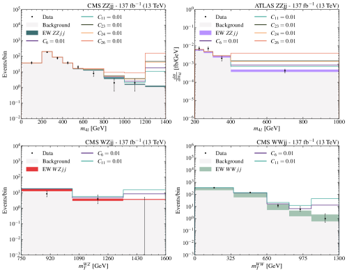
Figure 1: Kinematic distributions employed in the analyses. In each panel we show the SM prediction, the data and the predictions for some illustrative values of the Wilson coefficients of the operators considered.

For illustration, we show in Fig. 1 the kinematic distributions used in our analyses together with the predictions for some values of the Wilson coefficients. As seen in this figure for all distributions studied, the observations and SM predictions agree with remarkable accuracy. Consequently, the data can be used to place bounds on the new physics effects. As expected, the effect of the new operators is most relevant in the highest invariant mass bins. This brings up the issue of possible violation of unitarity. We will come back to this point when discussing the derived bounds.

To derive the bounds on the Wilson coefficients of the operators, we build our test statistics $\chi^{2}$ function for each of the channels following the details provided by the experimental collaborations. As mentioned above, the experimental collaborations have performed their searches for QGC in the framework of dimension-eight SMEFT operators. Thus, for each channel we have tested our $\chi^{2}$ function by performing first the analysis with dimension-eight SMEFT operators to compare the sensitivity obtained with our fit and the one obtained by the collaborations. In this respect, it is important to notice that both the analysis of $W^{\pm}W^{\pm}jj\to\ell^{\pm}\nu\ell^{\prime\pm}\nu jj$ and $WZjj\to\ell^{+}\ell^{-}\ell^{\prime}\nu jj$ events by CMS [25] and of $ZZjj\to\ell^{+}\ell^{-}\ell^{\prime+}\ell^{\prime}jj$ by ATLAS  [38] are performed by the collaborations using two-dimensional distributions of the invariant mass closely related to the diboson ($M_{T}^{WW}$, $M_{T}^{WZ}$, or $m_{4\ell}$) and the dijet invariant mass $m_{jj}$. But there is not enough information in the publications about the correlations between the two-dimensional distributions to reproduce such analyses. Therefore, we make use of the one-dimensional distribution of the diboson-related invariant mass and, in consequence, our bounds are consistent with those obtained by the collaborations though slightly weaker.

In brief:

• For the analysis of the CMS $ZZjj\to\ell^{+}\ell^{-}\ell^{\prime+}\ell^{\prime-}jj$ channel [24], the number of events is large enough to assume gaussianity once the contents of the last four bins are combined. Thus, in this case we define

  $$\chi^{2}_{ZZ,\rm CMS}(C_{6},C_{11},C_{23},C_{24},C_{26})=\sum_{i=1}^{6}\dfrac{(N^{\text{obs}}_{i}-N^{\text{th}}_{i})^{2}}{\sigma_{i}^{2}}$$ (11)

  where, for bin $i$, $N^{\text{obs}}_{i}$ is the observed number of events and the expected number of events is given by

  $$N_{i}^{\rm th} = N_{i}^{\text{signal}}+N_{i}^{\text{backg}}\hskip 28.45274pt{\rm with}\hskip 28.45274ptN_{i}^{\text{signal}}=N_{i}^{\text{SM}}+N_{i}^{\text{Int}}+N_{i}^{\text{BSM}},$$

  where by $N_{i}^{\text{SM}}$, $N_{i}^{\text{Int}}$ and $N_{i}^{\text{BSM}}$ we denote the expected number of $ZZjj$ events from the SM contribution, the interference of the SM and HEFT ${\cal O}(p^{4})$ amplitudes and the squared amplitudes generated by the ${\cal O}(p^{4})$ HEFT operators, respectively. $\sigma_{i}$ contains the statistical and uncorrelated theoretical and systematic uncertainties added in quadrature $\sigma_{i}^{2}=N^{\text{obs}}_{i}+(0.07\times N^{\text{th}})^{2}$.

• For the analysis of the CMS $W^{\pm}W^{\pm}jj\to\ell^{\pm}\nu\ell^{\prime\pm}\nu jj$ process we use the $\chi^{2}$ function

  $$\chi^{2}_{WW,\rm CMS}(C_{6},C_{11})=\min_{\vec{\xi}}\Big{\{}2\sum_{i=1}^{5}\Big{[}N_{i}^{\text{th}}(\vec{\xi})-N_{i}^{\text{dat}}+N_{i}^{\text{dat}}\log\Big{(}\dfrac{N^{\text{dat}}_{i}}{N^{\text{th}}_{i}(\vec{\xi})}\Big{)}\Big{]}+\sum_{i}\xi_{i}^{2}\Big{\}}$$ (12)

  where we introduce two pulls $\xi_{1}$ and $\xi_{2}$ to account for the theoretical and systematic uncertainties of the signal and background events, so

  $$N_{i}^{\rm th}(\vec{\xi})=N_{i}^{\text{signal}}(1+\sigma^{\xi_{1}}_{i}\,\xi_{1})+N_{i}^{\text{backg}}(1+\sigma^{\xi_{2}}_{i}\,\xi_{2})$$ (13)

  with $\sigma^{\xi_{1}}_{i}=\sigma^{\xi_{1}}_{i}=0.07$ for $i=1,2,3$.

• For the analysis of the CMS $WZjj\to\ell^{+}\ell^{-}\ell^{\prime}\nu jj$ events in Ref. [25] we focus on the last three bins from which we build

  $$\chi^{2}_{WZ,\rm CMS}(C_{6},C_{11},C_{23},C_{24})=\min_{\vec{\xi}}\Big{\{}2\sum_{i=1}^{3}\Big{[}N_{i}^{\text{th}}-N_{i}^{\text{dat}}+N_{i}^{\text{dat}}\log\Big{(}\dfrac{N^{\text{dat}}_{i}}{N^{\text{th}}_{i}}\Big{)}\Big{]}+\sum_{i}\xi_{i}^{2}\Big{\}}$$ (14)

  with $\sigma^{\xi_{1}}_{i}=0.25,0.30,0.35$ and $\sigma^{\xi_{2}}_{i}=0.15,0.2,0.25$ for $i=1,2,3$ respectively.

• For the analysis of the ATLAS $ZZjj\to\ell^{+}\ell^{-}\ell^{\prime+}\ell^{\prime-}jj$ channel [38] the observable we use is the four-lepton invariant-mass differential cross section ($d\sigma/dm_{4l}$) which is a particle-level distribution, hence, in obtaining our predictions we need to simulate the production, decay, and perform the parton-shower and hadronization, but detector effects do not need to be simulated. In this case we build the statistics

  $$\chi^{2}_{ZZ,\rm ATLAS}(C_{6},C_{11},C_{23},C_{24},C_{26})=\sum_{i=i}^{4}\dfrac{(S^{\text{obs}}_{i}-S^{\text{th}}_{i})^{2}}{\sigma_{i}^{2}},$$ (15)

  where we read the values of $S^{\text{obs}}_{i}$ from the data points in Fig. 4 of Ref. [38]. The theoretical predictions for the differential cross section in each bin $i$ is obtained from the generated number of events with the proper normalization and it has the contributions

  $$S_{i}^{\text{th}}=S_{i}^{\text{SM,signal}}+S_{i}^{\text{Int,signal}}+S_{i}^{\text{BSM,signal}}+S_{i}^{\text{backg}}\;.$$ (16)

  The uncertainties in Eq. (15) are $\sigma_{i}=(0.3,0.3,0.3,0.4)\times S^{\text{obs}}$ for $i=1,4$.

Finally, we define the statistics for the global analysis

$$\chi^{2}_{\rm GLOBAL}(C_{6},C_{11},C_{23},C_{24},C_{26})=\chi^{2}_{ZZ,\rm CMS}+\chi^{2}_{WW,\rm CMS}+\chi^{2}_{WZ,\rm CMS}+\chi^{2}_{ZZ,\rm ATLAS}\;.$$ (17)

IV Results and Discussion

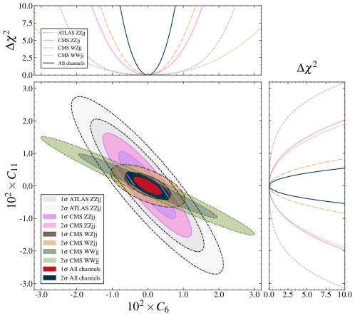
Figure 2: One- and two- dimensional projections of $\Delta{\chi}^{2}$ for the Wilson coefficients of the two $SU(2)_{C}$ conserving operators. We present the analyses of the different channels and their global combination as indicated in each panel after marginalizing over the undisplayed parameter.

We perform first an analysis of the data described in the previous section including the effect of the operators which conserve the custodial $SU(2)_{C}$, i.e. ${\cal P}_{6}$ and ${\cal P}_{11}$. We plot in Fig. 2 the 68% and 95% CL two-dimensional allowed regions for their Wilson coefficients, and the corresponding one-dimensional projections of the marginalized $\Delta\chi^{2}$ of the different channels studied and their combination. From the figure we see how the inclusion of channels involving different gauge boson pairs is important to break the partial degeneracies between the effect of both operators in each individual channel. From the one-dimensional projections we read the corresponding allowed ranges which at 95% CL are:

$$-0.0050\leq C_{6}\leq 0.0049\;,$$ (18)

$$-0.0034\leq C_{11}\leq 0.0035\;.$$ (19)

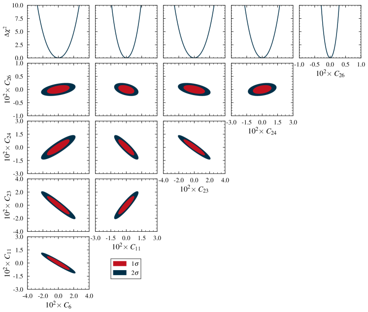
Figure 3: One- and two- dimensional projections of $\Delta{\chi}^{2}_{\rm GLOBAL}$ for the Wilson coefficients of the five operators as indicated in each panel after marginalizing over the undisplayed parameters.

We then perform the analysis involving the effect of the five operators. In this most general case, to obtain closed bounds in the five-dimensional parameter space, one needs to combine the data of all channels in order to break the exact degeneracies existing in some of the individual channels. The results of the analysis are shown in Fig. 3 where we present the one- and two-dimensional marginalized 68% and 95% CL allowed regions for the five Wilson coefficients. The corresponding 95% CL allowed ranges are listed in the right column in Table 2. As seen in the figure, even with the combination of the four channels, there remain large correlations or anti-correlations between $C_{6}$, $C_{11}$, $C_{23}$, and $C_{24}$. The weakest correlations occur for the $C_{26}$ coefficient. As a consequence, the bounds on the custodial conserving coefficients $C_{6}$ and $C_{11}$ worsens by a factor ${\cal O}(4-5)$ when including the the effects of the $SU(2)_{C}$ violating operators in the analysis.

Coefficient	Individual	Marginalized
$C_{6}$	[-0.003, 0.003]	[-0.018, 0.018]
$C_{11}$	[-0.002, 0.002]	[-0.009, 0.009]
$C_{23}$	[-0.0024, 0.0025]	[-0.017, 0.017]
$C_{24}$	[-0.0023, 0.0024]	[-0.011, 0.011]
$C_{26}$	[-0.0013, 0.0013]	[-0.0019, 0.0020]

Table 2: 95% CL intervals for the Wilson coefficients in the analyses. The central column are the allowed confidence intervals obtained by setting all other coefficients to zero, while the right column are the results when marginalizing all other four parameters in the analysis.

For the sake of comparison, we have also performed the global analysis including only one operator at a time. The results are listed in the central column in Table 2. Comparing with the marginalized bounds they range from a factor 1.5 stronger for the least correlated coefficient, $C_{26}$, to a factor 10 tighter for $C_{23}$.

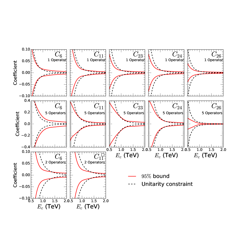
Figure 4: 95% CL allowed range for the 5 Wilson coefficients from our analyses (full red line) as a function of the cut-off energy. The upper panels correspond to the analysis in which only one non-vanishing operator is included in the analysis while in the central panels all five operators are included so the ranges shown in each panel are obtained after marginalization with respect to the other four coefficients. The lower panels depict the $SU(2)_{C}$ symmetric case. The dashed lines are the corresponding unitarity constraints in Eqs.(20) and (21).

All the results presented so far have been obtained including the contribution of the new operators without any constraint on the kinematic range of the analyzed distributions. This raises the issue of possible violation of unitarity. In Ref. [45] a dedicated study of partial-wave unitarity constraints on genuine QGC is presented for HEFT and SMEFT. The derived unitarity bounds read

$$C_{i}\leq\{1.25,1.96,1.19.,1.35.0.69\}\times 10^{-2}\times\left(\frac{\rm TeV}{\hat{s}}\right)^{2}\,,\;\;\;\left[\leq\{6.9,6.9,10.,10.,2.7\}\times 10^{-2}\times\left(\frac{\rm TeV}{\hat{s}}\right)^{2}\right]\,,$$ (20)

for $i=\{6,11,23,24,26\}$ when considering one non-vanishing operator at a time [all five operators simultaneously] and where $\hat{s}=m_{VV^{\prime}}^{2}$ is the square of the center-of-mass (COM) energy of the $2\rightarrow 2$ gauge-boson process. Also, with the expressions given in Ref. [45], one can derive that in the $SU(2)_{C}$ symmetric scenario, the unitarity bounds are

$$C_{i}\leq\{5.1,6.0\}\times 10^{-2}\times\left(\frac{\rm TeV}{\hat{s}}\right)^{2}\,,$$ (21)

for $i=\{6,11\}$. Therefore, from Table 2 we read that in the analysis with one operator different from zero at a time, unitarity can be violated for the extreme values of the allowed ranges for $\sqrt{\hat{s}}\geq\{1.4,1.7,1.5,1.6,1.6\}\,{\rm TeV}$ for $i=\{6,11,23,24,26\}$ and for $\sqrt{\hat{s}}\geq 1.4\,{\rm TeV}$ for the analysis including the effect of all five operators. In the $SU(2)_{C}$ symmetric case, the limits in Eqs. (19) imply that partial-wave unitarity is violated for $\sqrt{\hat{s}}\geq 1.8$ TeV.

Conservative bounds, which ensure unitarity conservation, can be obtained by repeating the analysis including the contribution of the anomalous operators to the observables only up to a hard kinematic cut-off $m_{VV^{\prime}}\leq E_{c}$ [46, 47] and by studying the dependence of the derived bounds on $E_{c}$. Then, the allowed range of coefficients is obtained for the maximum value of $E_{c}$ for which the unitarity constraint is saturated for the extreme values of the 95% CL allowed range. We plot in Fig. 4 the 95% CL allowed range of the five coefficients as a function of $E_{c}$ compared to the unitarity bound for the cases with one operator is non-vanishing (upper panels), with all operators included (central panels) and with the inclusion of the $SU(2)_{C}$ conserving operators only (lower panels).

One must notice that the unitarity constraints Eqs. (20) and  (21) do not hold a statistical significance and therefore with this procedure one is combining the statistically allowed ranges obtained by the analysis of the experimental data with certain CL, with a unitarity cut-off. So, the values obtained with this procedure can be taken mostly as an illustration of the loss of sensitivity when enforcing unitarity with this method. As seen in Fig. 4, the bounds when considering one operator at a time degrade by a factor 3-10 and by a factor ${\cal O}(10)$ when considering all operators at a time. In the $SU(2)_{C}$ conserving scenario, the allowed ranges od $C_{6}$ and $C_{11}$ become a factor $\sim 3$ and $\sim 5$ broader respectively.

In brief, we have obtained the bounds on genuine anomalous QGC generated at the lowest order in the HEFT using the presently available ATLAS and CMS experimental data on VBF production of gauge-boson pairs. We have considered three different scenarios varying in the number of operators involved in the analysis. We find that without imposing any unitarity restriction on the anomalous cross sections, the constraints on the Wilson coefficients are of the order of ${\cal O}(0.003)$ TeV^-4 for scenarios in which only one operator contributes at the time. In the $SU(2)_{C}$ symmetric case [all five operators simultaneously], the limits relax to ${\cal O}(0.005)$ [${\cal O}(0.02)$] TeV^-4. Next, we restudied the problem using a hard cut-off to guarantee that there is no unitarity violation and obtained the most stringent constraints without unitarity violation. Our results show that the limits on anomalous QCG are degraded by a factor ${\cal O}(3-13)$ when we enforce the anomalous amplitudes to respect unitarity, as expected. The same degradation must also occur in the present limits obtained by the experimental collaborations in the SMEFT scenario.