Full range spectral correlations and their spectral form factors
in chaotic and integrable models

Abstract

Quantum chaotic systems are characterized by energy correlations in their spectral statistics, usually probed by the distribution of nearest-neighbor level spacings. Some signatures of chaos, like the spectral form factor (SFF), take all the correlations into account, while others sample only short-range or long-range correlations. Here, we characterize correlations between eigenenergies at all possible spectral distances. Specifically, we study the distribution of $k$-th neighbor level spacings ($k$nLS) and compute its associated $k$-th neighbor spectral form factor ($k$nSFF). This leads to two new full-range signatures of quantum chaos, the variance of the $k$nLS distribution and the minimum value of the $k$nSFF, which quantitatively characterize correlations between pairs of eigenenergies with any number of levels $k$ between them. We find exact and approximate expressions for these signatures in the three Gaussian ensembles of random matrix theory (GOE, GUE and GSE) and in integrable systems with completely uncorrelated spectra (the Poisson ensemble). We illustrate our findings in a XXZ spin chain with disorder, which interpolates between chaotic and integrable behavior. Our refined measures of chaos allow us to probe deviations from Poissonian and Random Matrix behavior in realistic systems. This illustrates how the measures we introduce bring a new light into studying many-body quantum systems, which lie in-between the fully chaotic or fully integrable models.

I Introduction

Complex many-body quantum systems are at the heart of fields as diverse as quantum information, condensed matter, statistical mechanics, and high energy physics. These systems are deeply connected to random matrices, whose statistical spectral correlations are fully characterized by their underlying symmetries, as first found by Wigner and others studying heavy nuclei [1, 2, 3, 4] and verified experimentally [5]. Random matrices are also deeply connected to quantum chaos and capture the spectral correlations of non-integrable systems [6]. By contrast, such correlations are absent in non-chaotic, or integrable systems, whose spectrum behaves as if the energy levels were sampled independently—therefore referred to as Poissonian statistics [7]. The statistics of a spectrum and its energy correlations thus are a defining feature of chaotic behavior.

The most commonly studied spectral statistical property is the distribution of nearest-neighbor level spacings (nnLS). Its connection to the random matrix distribution is often taken as a defining feature of quantum chaos, even in many-body systems without a well-defined classical limit, and is expected to be universal—that is, independent of the system’s microscopic details. Still, physical systems can exhibit correlations all over their spectrum. The spectral form factor, detailed below, accounts for all spectral levels, and studies of long-range correlations have been introduced early on [8]. These include the spectral rigidity (how close the staircase function of an unfolded spectrum is to a straight line), the number variance (the variance in the number of levels in an interval of length $L$) [9, 10], and the $k$th closest neighbor spacing density [11]. Despite these various measures, long-range correlations remain much less studied than the distribution of nnLS. In this work, we characterize correlations between energies at all possible spectral distances and show that all correlations are important to correctly describe the dynamics of quantum chaotic systems. Importantly, we introduce two new signatures of quantum chaos based on full-range spectral correlations. These measures, which can be extracted from knowledge of the spectrum, provide a refined probe of quantum chaos, and open a window to studying systems in-between the fully chaotic or fully integrable models, where there may be correlations for nearest neighbours but less correlation for further away neighbours, or vice versa.

While the spectral statistics of certain systems are experimentally accessible [5], it was soon realized that it is subject to many sources of noise which could alter the measurements. The Fourier transform of the spectrum [12], which yields the spectral form factor (SFF), is not much affected by experimental errors while still being sensitive to spectral correlations through the correlation hole. The SFF thus now serves as a signature of quantum chaos [13, 14, 15, 16, 17, 18, 19, 20], and there have been proposals to measure it, see e.g. [21, 22]. Because the SFF is not a self-averaging quantity [23], it is customary to average over an ensemble or a small time window. For systems with energy correlations, the time evolution of the SFF displays an initial decay (the slope), reaches a minimum in the dip, starts growing back with a linear ramp, and finally saturates to a constant value—the plateau. The SFF contains information of all correlations between the energies as per its definition, and we will see that this is a requirement to describe the linear ramp. This characteristic evolution is taken as a signature of chaos, since integrable systems do not exhibit any linear ramp—they can decay directly to the plateau or show periodic oscillations in time. Regardless of whether the system is chaotic or not, the early time decay of the SFF is universally bounded [24]. Also, it can be used to set a universal bound on the quantum dynamics, which gives insight into thermalization and scrambling [25].

Quantities such as the nnLS and the SFF have received much attention; they are widely used and studied in the literature. The first accounts for the nearest energy neighbors only, while the second includes all energy levels and spectral distances. In a sense, these provide a signature of quantum chaos based on a figurative “black or white” spectral representation. Here, we look at all possible “shades of grey”, and characterize the effect of correlations between any neighbors in energy. This leads to two new signatures of quantum chaos. Specifically, we first compute the $k$-th neighbor Level Spacing ($k$nLS) distribution for all the Gaussian ensembles of Random Matrix Theory (RMT) and the Poissonian ensemble. We find that its variance is a good measure of the strength of energy correlations at a certain spectral distance. This variance exhibits a scaling that differs in the RMT and Poisson cases, and can therefore be used as a signature of quantum chaos. Secondly, each of the $k$nLS distribution has an associated $k$-th neighbor Spectral Form Factor ($k$nSFF), which we compute analytically for the RMT and Poissonian ensembles. We find that the minimum value of the $k$nSFF behaves very differently for the RMT and Poisson cases, providing us with another signature of chaos: specifically, the neighbor $k^{*}$ with the deepest $k$nSFF allows to probe the transition between chaos and integrability. All of our results in RMT are computed analytically for the three Gaussian ensembles, providing useful asymptotic expansions of those involving special functions, and compared with numerical simulations of random matrices.

We further characterize full-range spectral correlations in a physically relevant model. We do so by illustrating our results in an XXZ spin chain with disorder, a model which is often used in the context of many-body localization (see e.g. [26, 27, 28, 29, 30]), and whose SFF was studied e.g. in [31, 32, 33]. This system shows a transition from chaos to integrability as a function of the disorder strength. Thus, we test how much the chaotic and integrable phases can be described in terms of the RMT/Poisson spectral and dynamical signatures.

The scope of our work extends to the high-energy community. Indeed, interest in quantum chaos has revived because of its connections to high energy physics and holography. In particular, black holes have a finite entropy, given by the Bekenstein-Hawking entropy [34], which indicates they have a discrete spectrum—similar to that of a quantum system with a finite number of degrees of freedom. Black holes are also expected to have a chaotic spectrum, and hence they can be modeled as a strongly-interacting many-body chaotic quantum system [35, 36, 37, 38, 39]. Within the framework of the AdS/CFT correspondence, low-dimensional black holes are related to certain limits of the Sachdev-Ye-Kitaev model—a chaotic strongly-interacting many-body quantum system [36, 37, 40, 38, 16]. The above-mentioned universality property of quantum-chaotic systems implies that they will share properties with other such systems, including black holes [16].

The paper is structured as follows: Section II presents a summary of our main results and introduces the models we study. The derivations and implications are detailed in the rest of the paper. In Sec. III, we study spectral statistics, first giving a comprehensive derivation of the $k$nLS distribution in RMT, which we test numerically for RMT and the XXZ model, and then studying the role of uncorrelated levels by looking at the Poisson distribution. We show how the variance of the $k$nLS distribution can be used to diagnose quantum chaos, and discuss its results in the XXZ spin chain with disorder. In Section IV, we study dynamical signatures of chaos, in particular we introduce a decomposition of the SFF in terms of the above-mentioned $k$th neighbor level spacings. We provide new dynamical measures of quantum chaos at any given spectral distance and test our results against numerical data from Gaussian ensembles as well as from XXZ in the transition from chaos to integrability. We introduce a toy model whose spectrum has mixed features of spectral correlations, namely, only nearest-neighbor correlations according to the Wigner distributions of level spacings, and verify that its SFF does not exhibit a linear ramp. Section V details a dissipative protocol to measure correlation functions related to the $k$nSFF. Finally, Section VI provides conclusions and a discussion of our results as well as future directions in the light of this work.

Figure 1: Signatures of full-range spectral correlations for the XXZ model (solid blue lines), GOE (dashed red line) and Poisson (dashed black line). The colorscale shows different disorder strengths $W$. (a) Variance of the $k$nLS distribution as a function of the neighbor degree $k$ (b) minimum of the $k$nSFF as a function of the neighbor degree $k$, the colored dots mark the deepest $k$nSFF, (c) deepest $k$-th neighbors SFF $k^{*}$ as a function of the disorder strength, the colorscale marks the $\langle r\rangle$ parameter. The values of $k^{*}$ for GOE and Poisson are $k^{*}=11$ and $k^{*}=28$ respectively, which can be obtained from the expansions for $k^{*}$ (12), (13) respectively with $N=200$ which is the energy window size.

II Summary of main results:
Fine probes of quantum chaos

In this work, we consider Hermitian Hamiltonians, each with a finite discrete spectrum (or energy window) with $N$ eigenvalues, $\{E_{1},E_{2},\dots,E_{N}\}$, that we arrange in increasing order. We define the set of $k$th nearest-neighbor level spacings ($k$nLS) for $1\leq k\leq N-1$ as $\{s_{1}^{(k)},s_{2}^{(k)},\dots,s_{N-k}^{(k)}\}$, where $s_{i}^{(k)}=E_{i+k}-E_{i}$ for $1\leq i\leq N-k$ integer. For example, $k=1$ gives the usual set of nearest-neighbor spacings. We always unfold the spectrum so that the average distance between eigenvalues is equal to one, $\langle s^{(1)}\rangle=1$. Thus, it is expected that $\langle s^{(k)}\rangle=k$.

We model chaotic Hamiltonians as belonging to one of the three RMT Gaussian ensembles (GOE, GUE, and GSE, distinguished by the Dyson index $\beta=1,2,4$ respectively, Sec. II.4) since many realistic models of quantum chaotic systems exhibit similar spectral statistics. To model integrable systems, we study square matrices with eigenvalues taken from a uniform distribution which are completely uncorrelated; the nearest-neighbor distribution of such eigenvalues is known to follow a “Poisson” process (which we label with $\beta=0)$. We also study a physical model and quantify how closely it follows the RMT or Poissonian ensembles. We choose the XXZ spin-chain with a varying amount of disorder in on-site magnetic field, because this model is known to interpolate between chaos and integrability as a function of the disorder strength, as detailed further below—see Sec. II.4.

We first summarize the two novel measures of chaos versus integrability that we introduce based on (full-range) spectral correlations: (i) the variances of the $k$th neighbor distributions as a function of the spectral distance $k$ and the ensemble, indexed by the Dyson index $\beta$; (ii) the dip value of the $k$th neighbor SFF as a function of $k$, along with the neighbor degree $k^{*}$ for which the $k^{*}$th neighbor SFF has the deepest minimum. We give analytical expressions for the three Gaussian ensembles (GOE, GUE, and GSE) and for the Poisson ensemble. These quantities are illustrated in Fig. 1 for a chaotic system modeled by the GOE, an integrable system modeled with the Poisson ensemble, and the XXZ spin chain with disorder, which shows a crossover from chaos to integrability as a function of the disorder strength, $W$. The figure and presentation below show how the quantities we introduce measure energy correlations at any spectral distances, thus providing refined tools to diagnose quantum chaos.

II.1 Beyond Wigner’s surmise

The probability distribution of the nnLS ($k=1$) follows Wigner’s surmise, $\mathcal{P}_{\beta}(s)=C_{\beta}s^{\beta}e^{-A_{\beta}s^{2}}$. We first derive the probability distribution for any energy spacing $s^{(k)}$ and go beyond known results [41, 42, 43, 44, 45, 46] by characterizing its variance, which can probe spectral correlations.

As mentioned above, the average of the distribution of $s^{(k)}$ for an unfolded spectrum is centered around $k$. We normalize this average to unity and study the distribution of $\tilde{s}^{(k)}\equiv s^{(k)}/k$ . We show in Section III that for the three RMT Gaussian ensembles—GOE, GUE and GSE with $\beta=1,2$ and $4$ respectively—the $k$th neighbor level-spacing distribution follows

$$\mathcal{P}_{\beta}^{(k)}(\tilde{s}) \approx C_{\alpha}\,\tilde{s}^{\alpha}\,e^{-A_{\alpha}\tilde{s}^{2}},$$ (1)

where $\alpha$ implicitly depends on the energy spacing $k$ and the ensemble $\beta$ through

$$\alpha=\frac{k(k+1)}{2}\beta+k-1~{}.$$ (2)

The values of $C_{\alpha}$ and $A_{\alpha}$ are detailed in Eqs. (28b) and (28a), respectively.

The average of the distribution $\mathcal{P}_{\beta}^{(k)}(\tilde{s})$ is $\langle\tilde{s}\rangle=1$, and its variance is therefore

$$\Delta_{\beta}^{(k)}\equiv\langle\tilde{s}^{2}\rangle-\langle\tilde{s}\rangle^{2}=\frac{\alpha+1}{\alpha}\left(\frac{\omega_{k}}{k}\right)^{2}-1,$$ (3)

where $\omega_{k}$ is a frequency we introduce in Eq. (55) to describe the dynamics in RMT. For large $k$, the frequency $\omega_{k}$ scales linearly with $k$ and the variance behaves as

$$\Delta_{\beta}^{(k)}\xrightarrow[k\to\infty]{}\frac{1}{\beta k^{2}}+\mathcal{O}\left(\frac{1}{k^{3}}\right)~{}.$$ (4)

For a Poissonian ensemble (which we will label with $\beta=0$), the normalized $k$th neighbor spacing distribution reads

$$\mathcal{P}_{0}^{(k)}(\tilde{s}) = \frac{k^{k}}{(k-1)!}\,\tilde{s}^{k-1}e^{-k\tilde{s}}~{},$$ (5)

with a variance given precisely by

$$\Delta_{0}^{(k)}=\frac{1}{k}~{}.$$ (6)

Figure 2 presents the variance of the $k$th level distribution for the three random matrix ensembles and the Poissonian ensemble, Eqs. (3) and (6) respectively, and shows a very good match with the numerical simulations. It clearly illustrates the distinctive behavior of the variance whether the system is chaotic or not. The variance of the distribution of normalized splittings $\tilde{s}$ decreases with $k$ because the normalization brings a $1/k^{2}$ factor—e.g. the variance of $\mathcal{P}_{0}^{(k)}(s)$ scales as $k$ while that of $\mathcal{P}_{0}^{(k)}(\tilde{s})$ scales as $1/k$, Eq. (6). The variance of the Poisson ensemble decays more slowly as a function of $k$ than that of chaotic RMT ensembles. This can be understood because the energies in the Poisson ensemble are completely uncorrelated while those in the other RMT ensembles are strongly correlated and thus spacing distributions cannot be as broad. The variance is thus a measure of the strength of energy correlation, and can be used to distinguish systems with integrable or chaotic spectral statistics. This phenomenon can also be understood as a smaller variance giving a more rigid spectrum in which eigenvalues have less possible values to be in.

Figure 1(a) shows how a physical model, as described by the XXZ spin-chain with disorder, interpolates between the results from the GOE (Eq. (3) with $\beta=1$) and the Poissonian ensemble (6), as a function of $W$. The variance we introduce allows to quantify the validity of the Bohigas-Giannoni-Schmit (BGS) [6] and Berry-Tabor (BT) [7] conjectures for the full-range of energy correlations, beyond only short-range or long-range measures. The deviations between the chaotic phase of the XXZ model and the GOE shows that $k$nLS distributions in the spin chain has a slightly larger variance for large $k$, so its energies are less correlated than the ideal chaotic model; similarly, the deviations between the integrable phase and the Poisson results can be understood as the XXZ energies being more correlated than the BT conjecture predicts, since the XXZ $k$nLS distributions exhibit a smaller variance than the Poisson ensemble for large $k$. The latter behavior can be understood in the large disorder case, see Sec. III.3 for a discussion.

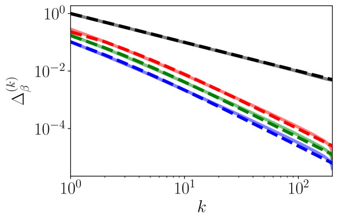
Figure 2: Variance of the distributions $\mathcal{P}_{\beta}^{(k)}(\tilde{s})$ as a function of spectral distance $k$. Dashed lines represent analytical results for the RMT ensembles (3) (with $\beta$=1 for the GOE, red; $\beta$=2 for the GUE, green; and $\beta$=4 for the GSE, blue) and Poisson distribution (6) (black). Continuous lines represent numerical results. The decay of the variance with the spectral distance is characteristic of spectral correlations, see main text. The plot uses matrices of dimension $N=200$ taking all of the eigenvalues into account, we average over $N_{\mathrm{av}}=2000$ elements of the ensembles.

II.2 The dip value of the $k$th neighbor SFF

The SFF is the simplest nontrivial measure of spectral correlations and indistinguishably accounts for all energy neighbors. It is defined from the Fourier transform of the two-level correlation function, namely, at infinite temperature, $S_{t}=\sum_{m,n}^{N}e^{-i(E_{n}-E_{m})t}/N^{2}$. We are here interested in characterizing the contribution of each $k$nLS to the SFF, and in a similar spirit to Wilkie and Brumer [13], we define the $k$th neighbor SFF ($k$nSFF) as

$$S^{(k)}_{t}\equiv\frac{2}{N^{2}}\Big{\langle}\sum_{i=1}^{N-k}\cos\,[t\,s_{i}^{(k)}]\Big{\rangle}~{},$$ (7)

where $N$ is the size of the matrix or the dimension of the Hilbert space in the case of a real system. In practice, $N$ will represent a window of energies around the densest part of the spectrum (before unfolding). The angular brackets denote an ensemble average, that, in the case of random matrices, is over random matrix realizations taken from the relevant ensemble, while in the XXZ model, it is over disorder realizations.

We find that the minimum value of the $k$nSFF, $S^{(k)}_{t_{d}}$, behaves differently in chaotic and integrable models. From our analysis, detailed in later sections, we find an approximation for the time at which the $k$nSFF has the first dip $t_{d}^{(k)}$, i.e. the $k$th dip time

$$t_{d}^{(k)} \approx \frac{\pi}{k}.$$ (8)

Surprisingly, this time turns out to be independent of the type of ensemble (i.e. Gaussian random matrices or Poisson) for an unfolded spectrum, as we show in Section IV from the expressions for the $k$nSFFs. In turn, the value of the $k$th neighbor SFF at the dip time does depend on the ensemble. For the Gaussian ensembles, we find

$$S_{t_{d}}^{(k)} \approx -\frac{2(N{-}k)}{N^{2}}e^{-\frac{\pi^{2}}{2k(\beta k+\beta+2)}}.$$ (9)

For the Poissonian ensemble, it reads

$$S_{t_{d}}^{(k)}=\frac{2(N-k)}{N^{2}}\cos^{k}\left(\frac{\pi}{1+k}\right)\cos\left(\frac{k\pi}{1+k}\right).$$ (10)

Figure 3 presents our analytical results for the Gaussian RMT and Poissonian ensembles, Eqs. (9) and (10), respectively, and shows the very good match with numerical results. We verify in Fig. 1(b) that the XXZ model with disorder interpolates between the GOE result (9) (with $\beta=1$) and the Poissonian result (10) as function of the strength of disorder. Note that for $k=1$, the Poisson spectra shows $S_{t_{d}}^{(1)}=0$, i.e. the Poisson nearest-neighbor SFF has no dip since $\cos\frac{\pi}{2}=0$. This can be understood from the lemma in [13] which states that the ($k$n)SFF of a distribution $\mathcal{P}(s)$ with a global maximum at $s=0$ is always lower bounded by its long time limit, i.e. there is no correlation hole. In this case, the nnLS distribution of the Poisson ensemble $\mathcal{P}^{(1)}_{0}(s)=e^{-s}$ has a global maximum at $s=0$, so the 1nSFF shows no dip. However, for energy levels further apart, $k>1$, the distribution $\mathcal{P}^{(k)}_{0}(s)\sim s^{k-1}e^{-s}$ has a global maximum at $s^{*}>0$ and the corresponding $k$nSFF thus displays a small dip, whose depth is characterized by (10) and plotted in Fig. 3.

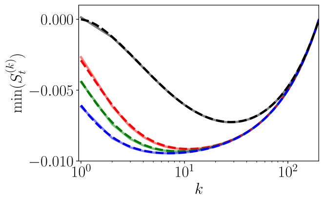
Figure 3: Minimum value of $k$nSFF $S_{t}^{(k)}$ as a function of the spectral distance $k$. Approximate analytical results (dashed lines) for the RMT ensembles (9) and Poisson distribution (10), and numerical results (solid lines). Colors are as in Fig. 2, i.e. Poisson (black), GOE (red), GUE (green) and GSE (blue). The numerical results are obtained from matrices of dimension $N=200$ and averaged over $N_{\mathrm{av}}=2000$ elements of the ensemble.

II.3 The deepest $k$th neighbor SFF

The complete SFF is composed of the $k$th neighbor SFFs,

$$S_{t}=\frac{1}{N}+\sum_{k=1}^{N-1}S^{(k)}_{t}~{},$$ (11)

where the first term originates from contributions of the zero frequencies and yields the above-mentioned “plateau”. One can ask for which spectral distance $k^{*}$ the $k$th neighbor SFF goes the deepest, i.e. for which $k$ the value of $S_{t_{d}}^{(k)}$ is the smallest, as a function of $\beta$ and $N$. The scaling of $k^{*}$ with $N$ can be found to follow

$$k^{*}\sim\mathcal{C}_{\frac{1}{3}}N^{\frac{1}{3}}+\mathcal{C}_{0}+\mathcal{C}_{-\frac{1}{3}}N^{-\frac{1}{3}}+\mathcal{O}(N^{-\frac{2}{3}})$$ (12)

for RMT ensembles, where the coefficients depend on $\beta$ and are given in Eq. (70).

For the Poissonian ensemble, however, this scaling is given by

$$k^{*}\sim\frac{\pi}{\sqrt{2}}N^{\frac{1}{2}}-\left(1+\frac{\pi^{2}}{4}\right)+\mathcal{O}(N^{-\frac{1}{2}}).$$ (13)

Figure 1(c) illustrates how the value of $k^{*}$ captures very well the XXZ spin chain transition from GOE to Poisson statistics as a function of the disorder strength. A commonly used single number indicator of chaos versus integrability in the spectrum, denoted $\langle r\rangle$, is defined as the average of the set $r_{i}=\textrm{min}\left(s^{(1)}_{i-1}/s^{(1)}_{i},s^{(1)}_{i}/s^{(1)}_{i-1}\right)$ [48, 49]. For systems with GOE statistics, $\langle r\rangle\approx 0.53$, while for systems with Poissonian level spacing statistics, $\langle r\rangle\approx 0.386$. As the disorder $W$ increases from values of order 1 to much larger values, the indicator for the considered spin chain displays a transition from the GOE value to the Poissonian value, thus witnessing a transition from chaotic to integrable system. As can be seen in Figure 1(c), the transition of $k^{*}$ is similar to that probed by the $\langle r\rangle$ parameter, as is indicated by the colorscale. Comparing with the colorscale, the transition from chaotic to integrable probed by $k^{*}$ appears to be broader than when probed by $\langle r\rangle$.

II.4 The models: chaotic, integrable, and the XXZ spin chain with disorder

As briefly mentioned, we model chaotic Hamiltonians as belonging to one of the three RMT Gaussian ensembles (GOE, GUE, and GSE) since many realistic models of quantum chaotic systems exhibit similar spectral statistics. These ensembles were introduced by Wigner [4], whose original idea to study heavy nuclei was to remove all specific details of the system to keep only their symmetries. He thus obtained Hermitian random matrices described by the Gaussian unitary ensemble (GUE); adding time-reversal symmetry ($[\hat{H},\hat{\mathcal{T}}]=0$ with $\hat{\mathcal{T}}$ the anti-unitary time reversal operator) lead to the Gaussian orthogonal ensemble (GOE) for $\hat{\mathcal{T}}^{2}=\mathbb{1}$, or the Gaussian symplectic ensemble (GSE) for $\hat{\mathcal{T}^{2}}=-\mathbb{1}$.

A Gaussian random matrix can be described by the joint probability density of its $N$ eigenvalues, which reads [8]

$$\rho(E_{1},\dots,E_{N})=C\!\!\!\prod_{1\leq i<j\leq N}\!\!|E_{i}-E_{j}|^{\beta}\,e^{-A\,\sum_{i=1}^{N}E_{i}^{2}},\quad$$ (14)

where $\beta$ is the Dyson index distinguishing the different ensembles, namely $\beta=1,2,4$ for the GOE, GUE, GSE, respectively. The constant $C$ is irrelevant in this work and $A$ sets the energy scale, which we keep free for now. Within the framework of random matrix theory, the Gaussian ensembles are constructed by sampling the matrix elements from Gaussian distributions in specific ways, that we detail in Appendix A for completeness. In particular, the matrix elements are sampled from the normal distribution with zero average and unit variance, $\mathcal{N}(0,1)$.

To model integrable systems, we study square matrices with eigenvalues taken from a uniform distribution which are completely uncorrelated; the nearest-neighbor distribution of such eigenvalues is known to follow from a Poisson process.

We also study a physical model and quantify how closely it follows the RMT or Poissonian ensembles. We choose the XXZ spin chain with a varying amount of disorder in on-site magnetic field, $\hat{H}=\hat{H}_{\textsc{xxz}}+\hat{H}_{\text{dis}}$, because this model is known to interpolate between chaos and integrability as a function of disorder strength. Specifically, the XXZ spin-chain Hamiltonian for $L$ spins reads

$$\hat{H}_{\textsc{xxz}}=\sum_{n=1}^{L}\big{[}\hat{S}_{n}^{x}\hat{S}_{n+1}^{x}+\hat{S}_{n}^{y}\hat{S}_{n+1}^{y}+J_{z}\hat{S}_{n}^{z}\hat{S}_{n+1}^{z}\big{]},$$ (15)

where $\hat{S}_{n}^{x,y,z}$ are spin 1/2 operators on site $n$. We assume periodic boundary conditions. This model is known to be integrable and can be solved using the Bethe ansatz [50]. Its spectrum follows Poissonian level spacing. Adding on-site magnetic fields with random strengths

$$\hat{H}_{\text{dis}}=\sum_{n=1}^{L}h_{n}^{z}\hat{S}_{n}^{z},$$ (16)

where $h_{n}^{z}$ are real random numbers taken from a uniform distribution $\mathcal{U}_{[-W/2,W/2]}$, changes the integrability properties of the XXZ chain as a function of the disorder strength $W$. Roughly speaking, when $W$ is small (but not too small), integrability is broken, while as $W$ increases, integrability is restored. The chaotic phase matches with the GOE statistics due to the system’s time-reversal symmetry: for $\hat{\mathcal{T}}=\hat{\mathcal{U}}\hat{\mathcal{K}}$ the anti-unitary time-reversal operator, generally written as the product of a unitary and complex-conjugation but which can be chosen as $\hat{\mathcal{T}}=\hat{\mathcal{K}}$ [51], we verify that $\hat{\mathcal{T}}\hat{H}\hat{\mathcal{T}}^{-1}=\hat{H}$ since the Hamiltonian is real. Studies of the SFF for this model can be found in [33]. The XXZ Hamiltonian with the disorder term (16) conserves the total spin in the $z$-direction; in other words, it commutes with the operator $\hat{\mathcal{S}}^{z}=\sum_{n=1}^{L}\hat{S}_{n}^{z}$. The Hamiltonian thus does not mix sectors of different $\hat{\mathcal{S}}^{z}$ eigenvalues, and we can work in one such sector. We choose to work in the sector with half of the spins up and half of the spins down, which is of dimension ${{L}\choose{L/2}}$. We present results for $L=16$ for which the Hilbert space dimension in the above-mentioned sector is $12{,}870$. In practice however, we draw our statistics from $N=200$ eigenvalues around the densest part of the spectrum.

III Spectral statistics

We now detail how to derive and characterize the $k$th-neighbor distributions for Gaussian random matrix ensembles as well as for the Poissonian ensemble.

III.1 Gaussian random matrix ensembles

We look for the probability distribution of the $k$th level spacing, $\mathcal{P}^{(k)}(s)$. Let us start with $k=1$. For a random matrix taken from a Gaussian ensemble (GOE, GUE or GSE), the nearest-neighbor level spacings $\{s_{i}^{(1)}\}_{i=1}^{N-1}$ of the unfolded spectrum (see Appendix C) are very well approximated by random variables taken from the Wigner surmise distribution,

$$\mathcal{P}^{(1)}_{\beta}(s) = C_{\beta,1}\,s^{\beta}\,e^{-A_{\beta,1}s^{2}},$$ (17)

where $C_{\beta,1}$ and $A_{\beta,1}$ are constant in $s$ and depend only on $\beta$ (since $k=1$); they are set by the conditions that $\mathcal{P}^{(1)}(s)$ is normalized and that the average level spacing is equal to unity, $\langle s\rangle=\int_{0}^{\infty}s\,\mathcal{P}^{(1)}(s)ds=1$.

This result can be derived by considering the distribution of the spacing $|E_{2}-E_{1}|$ between the eigen-energies of a $2\times 2$ random matrix, which is the smallest possible random matrix to have a nearest-neighbor spacing. As Wigner rightly conjectured [4], this is a good approximation to the level spacing distribution also for matrices with $N>2$; the distribution of nearest-neighbor level spacings in a Gaussian random matrix of any size very closely follows his surmise, provided that the spectrum is unfolded.

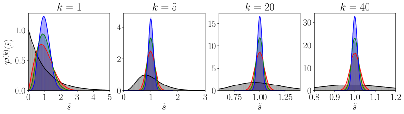
Figure 4: $k$-th neighbor level spacing distribution for the Poisson (black), GOE (red), GUE (green), and GSE (blue) ensembles for different spectral distances $k=1,5,20,40$. The analytical Wigner surmise (lines) we derive, Eqs. (39) and (1), is in perfect agreement with the unfolded numerical data (histogram). Numerical results are obtained averaging over $N_{\mathrm{av}}=1000$ realizations of random matrices of dimension $N=100$. The variances of these distributions are shown in Fig. 2 and can serve as an indicator to distinguish between integrable and chaotic systems.

For energy levels further apart, we follow Wigner’s footsteps and use the smallest possible random matrix ensemble with that particular spectral distance. Specifically, to find the distribution of the $k$th neighbor level spacing, $s^{(k)}$, we use an $N=k+1$ dimensional random matrix with energy levels $E_{1}\leq E_{2}\leq\dots\leq E_{k+1}$ and look for the distribution

$$\mathcal{P}^{(k)}(s) =\int_{-\infty}^{\infty}\!\!dE_{1}\int_{E_{1}}^{\infty}\!\!dE_{2}\,\dots\int_{E_{k}}^{\infty}\!\!dE_{k+1}\rho(E_{1},\dots,E_{k+1})$$

$$\times\delta\big{[}s-(E_{k+1}-E_{1})\big{]},$$ (18)

where $\rho$ is the joint probability distribution (14), and where we have written the integration limits explicitly, taking into account the ordering of the levels. We conjecture that this is a good approximation for $\mathcal{P}^{(k)}$ for matrices with dimension $N>k+1$ and numerically show that it is appropriate.

Following the derivation in [52], we change variables from $\{E_{1},E_{2},\dots,E_{k+1}\}$ to $\{E_{1},s_{1},s_{2},\dots,s_{k}\}$, where $s_{i}\equiv s_{i}^{(1)}$ are all the nearest-neighbor spacings. So

$$\mathcal{P}^{(k)}(s) \propto\int_{-\infty}^{\infty}dE_{1}\int_{0}^{\infty}ds_{1}\dots\int_{0}^{\infty}ds_{k}\,\rho(E_{1},s_{1}\dots,s_{k})$$

$$\times\delta\Big{(}s-\sum_{i=1}^{k}s_{i}\Big{)},$$ (19)

where we omit the constant Jacobian which is not relevant in this work because we will eventually normalize the final result. Notice that $E_{1}$ appears only in the exponential term of $\rho(E_{1},s_{1}\dots,s_{k})=\big{[}p(s_{1},s_{2},\dots,s_{k})\big{]}^{\beta}\times e^{-A[E_{1}^{2}+(E_{1}+s_{1})^{2}+(E_{1}+s_{1}+s_{2})^{2}+\dots+(E_{1}+s_{1}+\dots+s_{k})^{2}]}$, written here with the $k(k+1)/2$ degree polynomial

$$p(s_{1},s_{2},\dots,s_{k}) =s_{1}(s_{1}+s_{2})\dots(s_{1}+s_{2}+\dots+s_{k})$$

$$\times s_{2}(s_{2}+s_{3})\dots(s_{2}+s_{3}+\dots+s_{k})$$

$$\times\dots\times s_{k-1}(s_{k-1}+s_{k})\times s_{k}~{}.$$ (20)

Since $s_{i}\geq 0$ for all $i$, this polynomial is positive everywhere. Performing the Gaussian integral over $E_{1}$, we find (up to an irrelevant constant)

$$\mathcal{P}^{(k)}(s) \propto\int_{0}^{\infty}ds_{1}\dots\int_{0}^{\infty}ds_{k}\big{[}p(s_{1},s_{2},\dots,s_{k})\big{]}^{\beta}$$

$$\times e^{-A\,q(s_{1},\dots,s_{k})}\,\delta\Big{(}s-\sum_{i=1}^{k}s_{i}\Big{)},$$ (21)

where we defined the quadratic polynomial resulting from the integration over $E_{1}$ as

$$q(\{s_{i}\})=\sum_{i=1}^{k}\frac{i(k+1-i)}{k+1}s_{i}^{2}+\sum_{i<j=1}^{k}\frac{2i(k+1-j)}{k+1}s_{i}s_{j}~{}.$$ (22)

Note that since $s_{i}\geq 0$ for all $i$ and the coefficients of this quadratic polynomial are always positive, we have $q(s_{1},\dots,s_{k})\geq 0$ everywhere. Next, we rescale the spacings through $x_{i}=s_{i}/s$. Taking into account the Jacobian of this transformation, which is $s^{k}$, the homogeneity of $p(s_{1},\dots,s_{k})$ and of $q(s_{1},\dots,s_{k})$, and using the delta function identity $\delta(ax)=\delta(x)/|a|$, we arrive at

$$\mathcal{P}^{(k)}(s) \propto s^{k-1}s^{\frac{k(k+1)}{2}\beta}\int_{0}^{\infty}dx_{1}\dots\int_{0}^{\infty}dx_{k}$$ (23)

$$\times\big{[}p(x_{1},x_{2},\dots,x_{k})\big{]}^{\beta}e^{-As^{2}q(x_{1},\dots,x_{k})}\,\delta\Big{(}1{-}\!\!\sum_{i=1}^{k}x_{i}\Big{)}.$$

This is an integral over a $(k-1)$ simplex. Using the $\delta$-function to set $x_{k}=1-x_{1}-x_{2}-\dots-x_{k-1}$ and restricting the integration limits, the quadratic function is replaced by $\overline{q}(\{x_{i}\}_{i=1}^{k-1})=\frac{k}{k+1}-2\sum_{i=1}^{k-1}B_{i}x_{i}+\sum_{i,j=1}^{k-1}A_{ij}x_{i}x_{j}$, the elements of the vector $\mathbf{B}$ and the matrix $\mathbf{A}$ being detailed in Appendix B; and we denote the change of the polynomial $p(\{x_{i}\}_{i=1}^{k})$ as $\overline{p}(\{x_{i}\}_{i=1}^{k-1})$. After completing the square, we arrive at the $(k-1)$-dimensional integral

$$\mathcal{P}^{(k)}(s) \propto s^{\frac{k(k+1)}{2}\beta}s^{k-1}e^{-\frac{A}{2}s^{2}}$$ (24)

$$\times\int_{0}^{1}dx_{1}\int_{0}^{1-x_{1}}dx_{2}\dots\int_{0}^{1-\sum_{i=1}^{k-2}x_{i}}dx_{k-1}$$

$$\times\big{[}\overline{p}(x_{1},x_{2},\dots,x_{k-1})\big{]}^{\beta}e^{-As^{2}(\mathbf{x}^{T}-\mathbf{m}^{T})\mathbf{A}(\mathbf{x}-\mathbf{m})},$$

where $\mathbf{m}=\mathbf{A}^{-1}\mathbf{B}$ and where we have used $A\big{[}\frac{k}{k+1}-\mathbf{B}^{T}\mathbf{A}^{-1}\mathbf{B}\big{]}=A/2$ for all $k$. It can be verified that $\mathbf{m}$ simplifies to $(1/2,0,\dots,0)$ which means that the Gaussian is centered at zero for all $x_{i}$ except $x_{1}$.

The integral over the simplex is challenging to compute exactly. For $s$ not too large, the Gaussian in the integral is flat enough to be considered independent of $s$ and yields a constant—we verified numerically that this is the case. The corrections at large $s$, where the Gaussian is peaked and within the integrating boundary of the simplex, are discussed below. In short, we found that the integral over the simplex brings corrections to the pre-factor Gaussian, deforming it slightly.

We can thus approximate the distribution of $k$nLS as

$$\mathcal{P}_{\beta}^{(k)}(s)\approx C_{\beta,k}\,s^{\alpha_{\beta,k}}\,e^{-A_{\beta,k}s^{2}}$$ (25)

with

$$\alpha_{\beta,k}=\frac{k(k+1)}{2}\beta+k-1~{},$$ (26)

and where the constants $C_{\beta,k}$ and $A_{\beta,k}$ are set by the normalization conditions during the unfolding process, see Eq. (28) below. Note that $\alpha_{\beta,k}\in\mathbb{N}$ for the all possible $k=1,2,\dots,N-1$ and $\beta\in\mathbb{N}$.

Since similar results have been reported in the literature, let us review their argument to contextualize our derivation. The first generalization of Wigner surmise that we are aware of assumes a Brody-like ansatz, which essentially leaves the power-law $\alpha$ as a free parameter [42]. In Ref. [53], the power-law in (2) is found using a small $s$ expansion and the generalized Wigner surmise, Eq. (1), is obtained assuming a Gaussian behavior at large $s$. This approach is also followed in [45] in the context of 2D Poisson point processes. These references thus find the correct distribution through heuristic arguments. Formal results for the $k$nLS probability distribution can be obtained exactly using tools from RMT, see e.g. [8], and there are even connections between the different $k$nLS distributions [46]. Since these results are formal and exact, they lack an explicit expression for the $k$nLS distribution reminiscent of the Wigner surmise, which is itself an approximation [54]. More recently, an extension of these results to spacing ratios was tested numerically [44] but with no analytical proof. Lastly, Rao [41] claims to have an analytic derivation of the generalized Wigner distribution from the joint-probability-density of eigenvalues. However, since the energies are not ordered, the spacing $E_{k+1}-E_{1}$ need not be a $k$-th spacing. The same work also seems to suggest that the generalized Wigner distribution is the exact distribution of the $k$-th spacing, despite the latter being known as an approximation only, as can already be seen in exact small size results like [52, 55]. In turn, our derivation gives a derivation based on Wigner’s original argument, i.e. considering the joint probability density of eigenvalues of the largest possible matrix with a $k$-th spacing; we have explicitly stated the approximations involved in getting the generalized Wigner distribution and discuss the corrections to the distribution below.

The generalized Wigner surmise (1) has been obtained starting from the joint probability distribution of eigenvalues of RMT (14)—without unfolding. It gives a good approximation of the $k$nLS distribution for any matrix of size $N\geq k$, provided that the spectrum is unfolded. As in the case of Wigner’s surmise (17), unfolding the spectrum sets the constants $C_{\beta,k}$ and $A_{\beta,k}$ from the conditions

$$\int_{0}^{\infty}\mathcal{P}^{(k)}(\tilde{s})\,d\tilde{s} =1,$$ (27a)

$$\int_{0}^{\infty}\tilde{s}\,\mathcal{P}^{(k)}(\tilde{s})\,d\tilde{s} =1~{}.$$ (27b)

Here, we introduced the rescaled variables $\tilde{s}^{(k)}=s^{(k)}/k$, so that we can treat all the neighbor degrees $k$ on equal footage, since then $\langle\tilde{s}^{(k)}\rangle=1\;\forall k$; consequently, we can drop the $k$ index. The first condition normalizes the distribution, while the second condition sets the average spacing between a level and its $k$th neighbor to equal $1$, thus setting the dimensions of frequency to unity and rendering all of our results dimensionless. We will undo this rescaling later in our discussion of the SFF.

The values of $C_{\beta,k}$ and $A_{\beta,k}$ are then given by

$$A_{\beta,k} =\left[\frac{\Gamma\left(\frac{\alpha_{\beta,k}}{2}+1\right)}{\Gamma\left(\frac{\alpha_{\beta,k}+1}{2}\right)}\right]^{2}$$ (28a)

$$C_{\beta,k} =\frac{2}{\Gamma\left(\frac{\alpha_{\beta,k}+1}{2}\right)}\left[\frac{\Gamma\left(\frac{\alpha_{\beta,k}}{2}+1\right)}{\Gamma\left(\frac{\alpha_{\beta,k}+1}{2}\right)}\right]^{\alpha_{\beta,k}+1}~{},$$ (28b)

where $\alpha_{\beta,k}$ is given in Eq. (2). For notational convenience, we write $\alpha\equiv\alpha_{\beta,k}$ and $A_{\alpha}\equiv A_{\beta,k},C_{\alpha}\equiv C_{\beta,k}$. Fig. 4 shows that our analytical results (1) perfectly capture the numerical simulation for all matrices of the Gaussian ensembles.

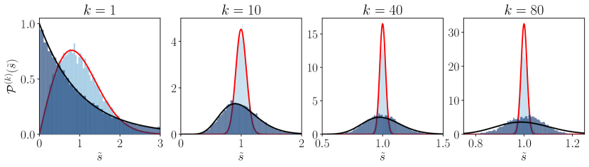
Figure 5: $k$-th neighbor level spacing distribution in XXZ for spectral neighbors, $k=1,10,40,80$, in the chaotic $W=1$ (light blue) and integrable $W=20$ (dark blue) phases along with the analytical results for Poisson (black line) and GOE (red line) models. The deviation between the integrable phase and Poissonian starts to be seen at $k=35$ and is very apparent at $k=70$ where the numerical distribution is much narrower. The considered XXZ model has $L=16$ spins in the zero magnetization sector $N_{u}=8$, the hopping is $J_{z}=2.21$, with PBC, the energy window size is $N_{\mathrm{en}}=200$ and the results include $N_{\mathrm{av}}=50$ disorder realizations. The variance of the distribution as function of $k$ is given in Fig. 1(a).

Expanding the expressions (28a) and (28b) in large $\alpha$ provides approximations for $A_{\alpha}$ and $C_{\alpha}$ that work particularly well when comparing with numerical results:

$$A_{\alpha} \approx\frac{\alpha}{2}+\frac{1}{4}+\frac{1}{16\alpha},$$ (29a)

$$C_{\alpha} \approx\frac{1+12\alpha}{12\sqrt{\pi\alpha}}e^{\frac{1}{2}+\frac{\alpha}{2}}~{}.$$ (29b)

From our definition (27b), the distribution $\mathcal{P}^{(k)}(\tilde{s})$ has average $\langle\tilde{s}\rangle=1$, and its variance is therefore

$$\Delta^{(k)}_{\beta}\equiv\langle\tilde{s}^{2}\rangle-\langle\tilde{s}\rangle^{2}=\left(\frac{\alpha+1}{2A_{\alpha}}\right)-1~{}.$$ (30)

For large $k$, this result behaves as

$$\Delta^{(k)}_{\beta}\xrightarrow[k\to\infty]{}\frac{1}{\beta k^{2}}+\mathcal{O}\left(\frac{1}{k^{3}}\right)~{}.$$ (31)

Note that, while Eq. (1) provides the distribution in a form that generalizes the Wigner surmise, we believe that a more physical expression of the $k$nLS distribution, which explicitly gives the width of the Gaussian, is obtained by defining $\kappa^{2}\equiv(\alpha+1)/2$ and reads

$$\mathcal{P}_{\beta}^{(k)}(\tilde{s})\approx\tilde{s}^{-1}\frac{2}{\Gamma(\kappa^{2})}\left(\kappa\frac{\tilde{s}}{\sqrt{\langle\tilde{s}^{2}\rangle}}\right)^{2\kappa^{2}}e^{-\kappa^{2}\frac{\tilde{s}^{2}}{\langle\tilde{s}^{2}\rangle}}$$ (32)

where we have used (30) to rewrite the constant (28a) as

$$A_{\kappa}=\left(\frac{\Gamma(\kappa^{2}+1/2)}{\Gamma(\kappa^{2})}\right)^{2}=\frac{\kappa^{2}}{\langle\tilde{s}^{2}\rangle}.$$ (33)

Corrections at large $s$.—As mentioned, we expect corrections to the generalized Wigner surmise (1) at large $s$. Starting back from Eq. (24), we can bound the resulting integral by a saddle-like approximation, namely, replacing $\overline{p}(x_{1},x_{2},\dots,x_{k-1})$ by its maximum $\overline{p}_{max}$ over the simplex. Since, at large $s$, the Gaussian has a very narrow peak (located on the boundary of the simplex), we can take the limits to infinity; the integral thus introduces an $s$-dependence of $(1/s)^{k-1}$. The probability distribution has a resulting $s$-dependence for large $s$ corrected as

$$\mathcal{P}^{(k)}(s)\xrightarrow[s\to\infty]{}s^{\frac{k(k+1)}{2}\beta}e^{-\frac{1}{2}As^{2}}~{}.$$ (34)

Note that, since the power $\frac{k(k+1)}{2}\beta$ is linear in $\beta$, this distribution can be interpreted as the Boltzmann factor of a Coulomb or ‘log gas’ [56, 57], which models a 1-dimensional array of atoms in a harmonic trap interacting with an effective potential taken as a logarithmic function of their distance. This interpretation as a log gas does not hold for the $\alpha$ coefficient in (2) because of zero-th order terms in $\beta$ that would need to be cancelled out with temperature-dependent interaction strengths in the effective model.

III.2 ‘Poisson’ ensemble: uncorrelated energy levels

We revisit the $k$th neighbor distribution for ensembles with uncorrelated energy levels, which we label with $\beta=0$ for convenience. This is known in the literature as the “Poissonian” case since its nearest-neighbor spectral statistics satisfy $\mathcal{P}^{(1)}(s)=e^{-\bar{\rho}s}$, where $\bar{\rho}$ is the average density of states, taken to be the uniform distribution $\bar{\rho}(E)=\bar{\rho}=1$. Assuming no correlations whatsoever between the energies, the joint probability distribution of the set of (uncorrelated) nearest-neighbor differences $\{s_{1},s_{2},\dots,s_{k}\}$ is just a product of the individual distributions,

$$\!\!P(s_{1},s_{2},\dots,s_{k})=P(s_{1})P(s_{2})\dots P(s_{k})=e^{{-}\!\sum_{i=1}^{k}s_{i}}.\,$$ (35)

As in the RMT case, the joint distribution $P(s_{1},s_{2},\dots,s_{k})$ allows us defining the probability that the $k$th nearest neighbor spacing is $s$ as

$$\mathcal{P}_{0}^{(k)}(s)\propto\int_{0}^{\infty}ds_{1}\dots ds_{k}\,P(\{s_{i}\}_{i=1}^{k})\delta(s-\sum_{i=1}^{k}s_{i}).\quad$$ (36)

This integral can also be carried out using rescaled variables $x_{i}=s_{i}/s$. The Jacobian brings a factor $s^{k}$ and the integration over the delta function contributes a $s^{-1}$ and sets everywhere $x_{k}=1-\sum_{i=1}^{k-1}x_{i}$. This yields

$$\mathcal{P}_{0}^{(k)}(s)\!\! {\propto} \!s^{k-1}e^{-s}\!\int_{0}^{1}dx_{1}\int_{0}^{1-x_{1}}\!dx_{2}\dots\int_{0}^{1-\sum_{i=1}^{k-2}x_{i}}\!\!dx_{k-1}$$ (37)

$$= s^{k-1}e^{-s}\times\textrm{constant}\,,$$

where the second equality follows from the fact that the integral over the simplex is a finite constant. The normalized distribution follows as

$$\mathcal{P}_{0}^{(k)}(s) = \frac{1}{(k-1)!}\,s^{k-1}e^{-s}~{}.$$ (38)

We verify that the average value of $\langle s\rangle=k$, as expected. Note that although for $k\geq 2$, the probability for very small $k$th spacing goes to zero, this does not reflect ‘level repulsion’ but rather reflects the fact that there is a small probability of having two levels that have $k-2$ levels between them be very close together. It is worth noting that the ‘repulsion’ of two such levels for the Gaussian ensembles goes like ${s}^{k-1+\frac{k(k+1)}{2}\beta}$, which is much stronger. To compare with the random matrix results from the previous section, we rescale $\tilde{s}\equiv s/k$ and find

$$\mathcal{P}_{0}^{(k)}(\tilde{s}) = \frac{k^{k}}{(k-1)!}\,\tilde{s}^{k-1}e^{-k\tilde{s}}~{}.$$ (39)

The mean of this distribution is $\langle\tilde{s}\rangle=1$ and the variance is

$$\Delta_{0}^{(k)}=\frac{1}{k}~{}.$$ (40)

Comparing this result with the large $k$ behavior of $\Delta_{\beta}^{(k)}$ (31), we see that the Gaussian RM ensemble $k$th neighbor distributions are much narrower that those of the completely uncorrelated (Poissonian) ensemble. Thus, the variance is a good indicator of the strength of spectral correlations.

III.3 Spectral statistics in the disordered XXZ model

To study the correlations in the spectrum and dynamical signatures of the XXZ spin chain with disorder, we average over many realizations of its Hamiltonian $\hat{H}=\hat{H}_{\text{XXZ}}+\hat{H}_{\text{dis}}$ for each value of $W$ and focus on a window in the densest part of the spectrum, upon which we perform global unfolding using a polynomial fit, detailed in App. C.

Figure 5 shows results for the distributions $\mathcal{P}^{(k)}(\tilde{s})$ for different values of $k$, comparing two different values of $W$: $W=1$ which corresponds to the chaotic phase of the model and $W=20$ which corresponds to the integrable phase. Figure 1 shows the variances of the distributions $\mathcal{P}^{(k)}(\tilde{s})$ as a function of $k$, as extracted from numerical data. Up to a certain value of $k$ both the chaotic and integrable phases follow the expected GOE and Poisson behavior, respectively. For larger $k$ we find deviations in both phases, particularly noticeable for the integrable phase, which can be understood as follows. For large disorder, the dominant contribution to the Hamiltonian is $\hat{H}_{\text{dis}}$, which on its own, can be thought of as a free, non-interacting Hamiltonian with energy levels given by $E_{i}=\sum_{n=1}^{L}\pm h_{n}^{z}$, with $i=1,2,\dots,N$. In the zero magnetization sector in which we are working, there are as many pluses as minuses. The energy level structure can be understood by ordering the $h_{n}^{z}$ according their absolute value. Then, the lowest energy level is obtained by distributing the $\pm$ such as to attribute minuses to the $|h_{n}^{z}|$ with larger values and pluses to the $|h_{n}^{z}|$ with smaller values. The highest energy level has the same structure but with pluses and minuses flipped. This small exercise shows that energy levels which are far away are actually correlated in $\hat{H}_{\mathrm{dis}}$, thus explaining the deviation from Poissonian statistics observed in Figures 1 and 5.

IV Dynamical signatures of chaos

In this section we turn to the effect of spectral statistics on dynamical quantities, focusing on the SFF. The SFF can be thought of as the simplest time-dependent observable which is a function of all energy differences in the spectral window. We introduce the $k$th neighbour SFFs and study their properties. We then sum them up (with appropriate coefficients) to obtain the complete SFF. In this process we learn about new structure which can be explained via the decomposition of the SFF into $k$nSFF components.

IV.1 The ensemble averaged $k$th neighbor SFF

The spectral form factor (SFF) is a time- and temperature-dependent quantity that probes the spectrum of a given quantum system. For a system at inverse temperature $\tilde{\beta}$, it is defined as $\mathcal{S}_{t}(\tilde{\beta})=|Z(\tilde{\beta}+it)/Z(\tilde{\beta})|^{2}$, with the partition function $Z(\tilde{\beta})=\sum_{i=1}^{N}e^{-\tilde{\beta}E_{i}}$ including all the energies $\{E_{i}\}_{i=1}^{N}$ of the Hamiltonian’s spectrum ($N$ can be infinite). In more detail,

$$\mathcal{S}_{t}(\tilde{\beta})=\frac{\sum_{i,j=1}^{N}e^{-\tilde{\beta}(E_{i}+E_{j})}e^{-it(E_{i}-E_{j})}}{\sum_{i,j=1}^{N}e^{-\tilde{\beta}(E_{i}+E_{j})}}~{}.$$ (41)

In the infinite temperature limit, $\tilde{\beta}\to 0$, the SFF becomes

$$\mathcal{S}_{t}(0)\equiv\mathcal{S}_{t}=\frac{N+2\sum_{i>j}\cos[t(E_{i}-E_{j})]}{N^{2}},$$ (42)

whose numerator can be divided into terms according to spectral distances $s_{i}^{(k)}$. This decomposition of the SFF is thus

$$\mathcal{S}_{t}=\frac{1}{N}+\sum_{k=1}^{N-1}\mathcal{S}^{(k)}_{t}~{},$$ (43)

and is formed by summing the k-th neighbor spectral form factors ($k$nSFFs)

$$\mathcal{S}^{(k)}_{t}\equiv\frac{2}{N^{2}}\sum_{i=1}^{N-k}\cos[t\,s_{i}^{(k)}]~{}.$$ (44)

As mentioned, the SFF is not self-averaging [23]; so we wish to compute the ensemble average $S_{t}=1/N+\sum_{k=1}^{N-1}\langle\mathcal{S}^{(k)}_{t}\rangle$, which boils down to computing the ensemble average of the individual contributions from each spectral distance, $\langle\mathcal{S}^{(k)}_{t}\rangle\equiv S_{t}^{(k)}$—also introduced earlier in the main results, Eq. (11). We show below a series of approximation that allow us to derive an analytical expression for the $S^{(k)}_{t}$ which provides a good approximation, and is obtained starting from the distributions $\mathcal{P}^{(k)}$ derived in Section III.

Figure 6: Time evolution of the $k$nSFF for Poisson (black), GOE (red), GUE (green) and GSE (blue) for different spectral neighbors, $k=1,5,20,40$ in systems of dimension $N=100$. The plots for $k=5,\;20,\;40$ show analytical results (thin lines) from (71) and (65), while for $k=1$ we show the exact expression (56), and numerical results for random matrices averaged over $N_{\mathrm{av}}=1000$ realizations (thick transparent lines). While we do not expect the approximation (65) to be good for small $k$, it works already quite well for GSE and $k=1$ and less so for GUE and GOE, in that order. Note the different scales in the time axis, chosen to better represent the increasing number of oscillations with the spectral neighbor $k$, see Eq. (64).

As discussed above, the ensemble average of the SFF can be decomposed according to the contributions from the various spectral spacings $k$. The latter can themselves be decomposed according to the energy levels $i$ as

$$S_{t}^{(k)}=\frac{2}{N^{2}}\sum_{i=1}^{N-k}\int dE_{1}\dots dE_{N}\,\rho(\{E_{i}\})\,\cos[t\,s_{i}^{(k)}].$$ (45)

Note that the energies $E_{i}$ are ordered. In a first step, we approximate all energy splittings $s^{(k)}_{i}=E_{i+k}-E_{i}$ as being independent of the absolute energy level and set $i=1$ as the reference level, so $s^{(k)}_{i}\rightarrow s^{(k)}_{1}$ and the sum over $i$ just becomes an $(N-k)$ factor. Then, in the same spirit as the $k$nLS distribution, we use the largest possible matrix which describes the $k$ level spacings and take $N\rightarrow(k+1)$. So we recognize the distribution of the $k$nLS, Eq. (III.1), and the $k$nSFF (45) thus becomes

$$S_{t}^{(k)} \approx\frac{2(N-k)}{N^{2}}\int ds^{(k)}\mathcal{P}^{(k)}(s^{(k)})\,\cos[t\,s^{(k)}],$$

$$\equiv C_{N}^{(k)}\,f^{(k)}_{t}~{},$$ (46)

where in the second line, we have introduced the following function and constant for later notational convenience:

$$f^{(k)}_{t} \equiv\int ds\,\mathcal{P}^{(k)}(s)\,\cos(t\,s)$$ (47a)

$$C_{N}^{(k)} \equiv\frac{2(N-k)}{N^{2}}.$$ (47b)

Let us mention that this result can be generalized. Indeed, the autocorrelation function at infinite temperature of any Hermitian operator $\hat{O}=\hat{O}^{\dagger}$ (i.e. any observable) can be decomposed in a similar manner using $f_{t}^{(k)}$ and changing only the coefficients $C_{N}^{(k)}$, as follows. Consider the autocorrelation function:

$$\mathcal{C}_{t}\equiv\frac{\mathrm{Tr}(\hat{O}\hat{O}(t))}{\mathrm{Tr}(\hat{O}^{2})}=\frac{1}{\mathcal{N}^{2}}\sum_{i,j=1}^{N}|O_{ij}|^{2}\cos\left[(E_{i}-E_{j})t\right],$$ (48)

where $O_{ij}$ are the matrix elements of the operator $\hat{O}$ in the energy basis and $\mathcal{N}^{2}=\sum_{i,j=1}^{N}|O_{ij}|^{2}$. The ensemble average of $\mathcal{C}_{t}$ can be decomposed into $k$th neighbor autocorrelation functions (see Appendix G for more details) as

$$C_{t}^{(k)}\equiv O_{N}^{(k)}\,f_{t}^{(k)}~{},$$ (49)

where $f_{t}^{(k)}$ are defined in (47a) and we define the coefficients:

$$O_{N}^{(k)}\equiv\frac{2}{\mathcal{N}^{2}}\sum_{i=1}^{N-k}|O_{i,i+k}|^{2}~{}.$$ (50)

An explicit relation between correlation functions and the $k$nSFF’s, along with a possible dissipative protocol to measure them, will be detailed in Sec. V.

We now turn to derive analytical expressions for $f_{t}^{(k)}$ (and for $S_{t}^{(k)}$) for the GOE, GUE and GSE as well as for completely uncorrelated energy levels (Poissonian ensemble).

IV.2 The $k$nSFF in Gaussian random matrix ensembles

With the (approximated) analytical result for $\mathcal{P}^{(k)}(\tilde{s})$ obtained in (1), we can look for an expression of the $k$nSFF $S^{(k)}_{t}$ for the Gaussian RM ensembles, starting from (46). We keep the rescaling of $\tilde{s}$ and rescale time according to $k$ to compute the integral (47a) as

$$f_{t}^{(k)} \equiv \!\!\int\!\!d\tilde{s}\,\mathcal{P}^{(k)}(\tilde{s})\cos(tk\,\tilde{s})$$

$$= \!\sum_{n=0}^{\infty}\frac{({-}1)^{n}}{(2n)!}(tk)^{2n}\langle\tilde{s}^{2n}\rangle$$

where

$$\langle\tilde{s}^{2n}\rangle =\int_{0}^{\infty}d\tilde{s}\,\tilde{s}^{2n}\,\mathcal{P}^{(k)}(\tilde{s})$$

$$=\left(\frac{\alpha+1}{2}\right)_{n}(A_{\alpha})^{-n}=\frac{(\kappa^{2})_{n}}{(A_{\kappa})^{n}},$$ (52)

where we have used the Pochhammer symbol $(a)_{n}=a(a+1)\dots(a+n-1)=\Gamma(a+n)/\Gamma(a)$. In turn, the function becomes

$$f_{t}^{(k)} = \sum_{n=0}^{\infty}\frac{\left(\frac{\alpha+1}{2}\right)_{n}}{(1/2)_{n}}\,\frac{\left(-(t\,k)^{2}/4A_{\alpha}\right)^{n}}{n!}~{}.$$ (53)

This sum can be expressed in terms of a hypergeometric function

$$f_{t}^{(k)} = e^{-\frac{k^{2}}{4A_{\alpha}}t^{2}}\,{}_{1}F_{1}\left(-\frac{\alpha}{2};\frac{1}{2};\frac{k^{2}}{4A_{\alpha}}t^{2}\right).$$ (54)

Since the coefficient $k/(2\sqrt{A_{\alpha}})$ appears in the $t$-dependent exponent, it is homogeneous to a frequency $\omega_{k}$. We thus set

$$\frac{k^{2}}{2A_{\alpha}}\equiv\frac{\omega^{2}_{k}}{\alpha},$$ (55)

and we will see that this quantity sets the width of the Gaussian envelope. The hypergeometric function can itself be expressed in terms of a Laguerre function, so we get

$$f_{t}^{(k)} = e^{-\frac{1}{2\alpha}\omega_{k}^{2}t^{2}}\,{}_{1}F_{1}\left(-\frac{\alpha}{2};\frac{1}{2};\frac{\omega_{k}^{2}t^{2}}{2\alpha}\right)$$ (56)

$$= \sqrt{\frac{\pi\alpha}{2}}\frac{k}{\omega_{k}}e^{-\frac{\omega_{k}^{2}t^{2}}{2\alpha}}L_{\alpha/2}^{-1/2}\left(\frac{\omega_{k}^{2}t^{2}}{2\alpha}\right).~{}$$

The Laguerre function, $L_{\mu}^{a}$ with $m-1<\mu<m$ for $m\in\mathbb{N}$ and $a>-1$, is defined by the infinite sum [59]

$$L_{\mu}^{a}(z) = \sum_{k=0}^{\infty}\binom{\mu+a}{\mu-k}\frac{(-z)^{k}}{k!}~{}.$$ (57)

When $\alpha$ is even, $\alpha=2m$ for $m\in\mathbb{N}$, in (56), the Laguerre function becomes a Laguerre polynomial of degree $m$:

$$L_{m}^{a}(z) = \sum_{k=0}^{m}\binom{m+a}{m-k}\frac{(-z)^{k}}{k!}~{}.$$ (58)

Since the degree of the Laguerre polynomial (or function, for non integer $\alpha/2$) grows quadratically with $k$, we can use the approximation for Laguerre polynomial of high degree :

$$L_{n}^{a}(x) = \frac{n^{a/2-1/4}}{\sqrt{\pi}x^{a/2+1/4}}e^{x/2}\Big{[}\cos(\theta_{a,n}(x))\left(1+\mathcal{O}\left(\frac{1}{n}\right)\right)$$ (59)

$$+\sin(\theta_{a,n}(x))\left(\frac{b_{a}(x)}{\sqrt{n}}+\mathcal{O}\left(\frac{1}{n}\right)\right)\Big{]}$$

where $\theta_{a,n}(x)=2\sqrt{nx}-a\pi/2-\pi/4$ and $b_{a}(x)=\big{(}4x^{2}-12a^{2}-24ax-24x+3\big{)}/(48\sqrt{x})$. Note that $b_{-1/2}(x)=\frac{\sqrt{x}}{12}(x-3)$.

In our case, we have a Laguerre polynomial of degree $n=\alpha/2$ (non necessarily integer), $a=-1/2$ and $x=\frac{\omega_{k}^{2}t^{2}}{2\alpha}$, so the above approximation reads

$$L_{\frac{\alpha}{2}}^{-\frac{1}{2}}(x)\approx\sqrt{\frac{2}{\pi\alpha}}e^{\frac{x}{2}}\Big{[}\cos\left(\omega_{k}t\right)+\frac{b_{-\frac{1}{2}}(x)}{\sqrt{\alpha/2}}\sin\left(\omega_{k}t\right)\Big{]}.$$ (60)

As can be seen in (59), the terms in the square brackets of (60) are an approximation up to (not including) $\mathcal{O}(1/\alpha)$. Thus, when plugging this result into (56) we must make sure that the combined coefficient of the square brackets is expanded to the same order in $\alpha$

$$\frac{1}{\sqrt{\alpha/2}}\frac{\Gamma(\alpha/2+1)}{\Gamma(\alpha/2+1/2)}=1+\mathcal{O}(1/\alpha)~{}.$$ (61)

Eventually, we find that $f_{t}^{(k)}$ can be approximated by

$$f_{t}^{(k)} = \Big{(}1+\mathcal{O}(1/\alpha)\Big{)}e^{-\frac{\omega_{k}^{2}t^{2}}{4\alpha}}$$

$$\times \Big{[}\cos(\omega_{k}t)+\sqrt{\frac{2}{\alpha}}{b_{-\frac{1}{2}}\left(\frac{\omega_{k}^{2}t^{2}}{2\alpha}\right)}\sin(\omega_{k}t)+\mathcal{O}(1/\alpha)\Big{]},$$

We note that the frequency defined through its introduction in Eq. (55) and rewritten below using Eq. (33), is well approximated at large $k$ by a linear function in $k$:

$$\omega_{k}=\sqrt{\frac{\alpha}{\alpha+1}\langle\tilde{s}^{2}\rangle}\>k\approx k-\frac{1}{2\beta k}+\mathcal{O}(1/k^{2})~{}.$$ (63)

Let us make several remarks about expression (IV.2):

• The initial value is always equal to unity, $f_{t=0}^{(k)}=1$ for all $k$;

• For $t\to\infty$, the overall exponential factor, $e^{-\frac{\omega_{k}^{2}t^{2}}{4\alpha}}$, makes $f_{t}^{(k)}\to 0$;

• $f_{t}^{(k)}$ is expressed as a sum of a cosine and a sine with the same frequency $\omega_{k}\to k$ at large $k$;

• Apart from the overall exponential factor, the coefficient of $\cos(\omega_{k}t)$ is $1$ while the coefficient of $\sin(\omega_{k}t)$ is time-dependent and is equal to $\sqrt{\frac{2}{\alpha}}\,b_{-1/2}\left(\frac{\omega_{k}^{2}t^{2}}{2\alpha}\right)=\frac{1}{12\alpha}\omega_{k}t\left(\frac{\omega_{k}^{2}t^{2}}{2\alpha}-3\right)$. It is of $\mathcal{O}(1/k)$ and thus of less consequence for large $k$. Note that, at the same time, it is more significant at large $t$. This is compatible with the fact that small $k$ terms (corresponding to low frequencies) are more significant at long time scales.

• We can compute the number of oscillations in one standard deviation of the envelope $\sqrt{2\alpha}/\omega_{k}$, by comparing it with the period of the oscillations $T_{k}=2\pi/\omega_{k}$. We thus find

  $$\frac{\sqrt{2\alpha}}{2\pi}\xrightarrow[k\to\infty]{}\frac{\sqrt{\beta}}{2\pi}k.$$ (64)

  So the number of oscillations of the $k$nSFF in the envelope is proportional to $\sqrt{\alpha}$, and scales linearly with the neighbor degree $k$ for large $k$, as illustrated in Fig. 6. The figure also illustrates that the largest number of oscillations that happen before the signal flattens because of the exponential decays is for the GSE, which has the largest $\beta$;

• Were the $k$nLS distribution a perfect Gaussian centered at $\langle s^{(k)}\rangle=k$, the $k$nSFF would only involve the Gaussian envelope and the cosine term $f_{t}^{(k)}=e^{-k^{2}t^{2}/(4\alpha)}\cos(kt)$ with frequency $\omega_{k}=k$, since the Fourier transform of a Gaussian is another Gaussian. The non-zero mean is accounted for by including $e^{i\langle s^{(k)}\rangle t}$, whose real part is $\cos(kt)$. Thus the sine term in the $k$nSFF comes from the non-gaussianity of the $k$nLS distribution. This is studied in more detail in App. D.

With the approximation (IV.2), the final expression for $S_{t}^{(k)}$ becomes

$$S_{t}^{(k)} \approx \frac{2(N-k)}{N^{2}}e^{-\frac{\omega_{k}^{2}t^{2}}{4\alpha}}\Big{[}\cos(\omega_{k}t)$$ (65)

$$+\frac{1}{12\alpha}\omega_{k}t\Big{(}\frac{\omega_{k}^{2}t^{2}}{2\alpha}-3\Big{)}\sin(\omega_{k}t)\Big{]}.$$

Figure 6 shows that our analytical approximation above very well reproduces the numerical data for all three Gaussian ensembles.

Before turning to the complete SFF, we study some more properties of the $k$th neighbor SFF: the “dip” time $t_{d}$ and depth of $S_{t}^{(k)}$ as a function of $k$, and the scaling of the deepest $k^{*}$ neighbor as a function of $N$.

IV.2.1 Dip time and depth of the $k$th neighbor SFF

We define the dip time for each $S_{t}^{(k)}$ as the time the function reaches its minimal value. It can be computed from the exact expression with $f_{t}^{(k)}$ given by (56), or from the approximate one, Eq. (65). However it may not be possible to analytically determine the minimum of those functions. One possibility to overcome this is to look at (65), where for large enough $k$ (and not too large $t$), the main contribution comes from the cosine. We know that its minimum happens when its argument is equal to $\pi$, therefore

$$t_{d}(k)\approx\frac{\pi}{\omega_{k}}\stackrel{{\scriptstyle\eqref{app_w_k}}}{{\approx}}\frac{\pi}{k}.$$ (66)

Note that this result suggests that the dip time does not depend on the ensemble $\beta$, but only on the neighbor degree $k$. For a more detailed analysis of this approximation, see Appendix F. From this estimate, we can also find the dip depth as a function of $k$, by plugging (66) into (65), and using (33), we find

$$S_{t_{d}}^{(k)} \approx -\frac{2(N{-}k)}{N^{2}}e^{-\big{(}\frac{\pi}{2}\frac{\kappa}{k}\frac{1}{\sqrt{2\langle\tilde{s}^{2}\rangle}}\big{)}^{2}}\!\!\!$$ (67)

$$\sim -\frac{2(N{-}k)}{N^{2}}e^{-\frac{\pi^{2}}{2k(\beta k+\beta+2)}}.\quad\>$$

Figure 7 shows that the approximation (66) for the dip time agrees with the numerical simulation from the different RMT ensembles, provided that the spectrum is unfolded.

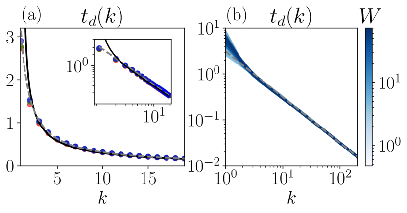
Figure 7: Dip time as a function of the neighbor degree for (a) ideal ensembles: Poisson (black), GOE (red), GUE (green) and GSE (blue) computed numerically from the unfolded spectrum along with the approximate expression (66) (dashed grey). Inset: same plot in log-log scale that shows explicitly the $t_{d}(k)\sim k^{-1}$ dependence; and (b) for the XXZ spin chain for different values of the disorder (blue colorscale) along with the analytical result $t_{d}(k)=\pi/k$ (dashed gray).

IV.2.2 Scaling of the deepest $k$-th neighbor SFF

The deepest $k$-th neighbor SFF, denoted by $k^{*}$, is computed from the minima of Eq. (67) for the Gaussian random matrix ensembles and (73) for the Poissonian ensemble (see next section). For random matrices, the deepest neighbor $k^{*}$ is the minimum of (67). It is challenging to extract the minimum from the exact expression. If we take the large $k$ approximation, we find the deepest $k^{*}$ to be given approximately by the solutions of

$$k^{*2}(2+\beta+\beta k^{*})=N\pi^{2},$$ (68)

whose exact solution can be found exactly using Mathematica but which is too cumbersome to understand. However, a large $N$ expansion yields

$$k^{*}\sim\mathcal{C}_{\frac{1}{3}}N^{\frac{1}{3}}+\mathcal{C}_{0}+\mathcal{C}_{-\frac{1}{3}}N^{-\frac{1}{3}}+\mathcal{O}(N^{-\frac{2}{3}})$$ (69)

for RMT ensembles, where the coefficients are given by

$$\mathcal{C}_{\frac{1}{3}} =\left(\frac{\pi^{2}}{\beta}\right)^{\frac{1}{3}},$$ (70a)

$$\mathcal{C}_{0} =-\frac{\beta+2}{3\beta},$$ (70b)

$$\mathcal{C}_{-\frac{1}{3}} =\frac{(2+\beta)^{2}-3\beta\pi^{2}}{9\beta^{\frac{5}{3}}\pi^{\frac{2}{3}}}.$$ (70c)

Figure 8 shows a good agreement between this expression and numerical random matrices for the three Gaussian ensembles.

Figure 8: Scaling of the deepest neighbor $k^{*}$ as a function of the system size $N$ computed numerically for RMT and Poisson ensembles (circles) and the analytical approximations (69) and (75) rounded to the nearest integer (lines). Numerical results are averaged over $N_{\mathrm{av}}=200$ matrices. The colors represent the different ensembles: black (Poisson), red (GOE), green (GUE) and blue (GSE). We show a guide for the eye at $N=200$ (gray dotted line) which agree with the values of $k^{*}$ used in Figure 1 for the Poissonian and GOE endpoints of $W$.

To end this section, we recall that the total SFF is not self averaging. We refer the reader to Appendix E which shows that the $k$nSFF for GUE (with similar conclusions for the other ensembles) is also not self-averaging.

IV.3 $k$th neighbor SFF for the Poissonian ensemble

The averaged $k$th neighbor SFF can be computed for matrices with uncorrelated eigenenergies, in the same manner as for the RM case, but now using the corresponding probability distribution, Eq. (39). We thus find

$$S_{t}^{(k)}=\frac{2(N-k)}{N^{2}}\frac{\cos(k\arctan t)}{(1+t^{2})^{k/2}}~{}.$$ (71)

The ‘dip’ time as a function of $k$, which we define to be the first minima of this function, can then be computed exactly as

$$t_{d}(k)=\tan\left(\frac{\pi}{1+k}\right)~{}.$$ (72)

Note that it asymptotically goes as $\pi/k$, similarly to the RMT case. The value of $\langle S_{t}^{(k)}\rangle$ at the dip time is

$$S_{t_{d}}^{(k)}=\frac{2(N-k)}{N^{2}}\cos^{k}\left(\frac{\pi}{1+k}\right)\cos\left(\frac{k\pi}{k+1}\right).$$ (73)

This expression admits the asymptotic expansion

$$S_{t_{d}}^{(k)}=\frac{2(N-k)}{N^{2}}\left(-1+\frac{\pi^{2}}{2k}-\frac{4\pi^{2}+\pi^{4}}{8k^{2}}+\mathcal{O}(k^{-3})\right),$$ (74)

which leads to a third-order polynomial equation whose solution can be expanded for large $N$. We thus find the deepest $k$nSFF to scale as

$$k^{*}_{0}\sim\frac{\pi}{\sqrt{2}}N^{\frac{1}{2}}-\left(1+\frac{\pi^{2}}{4}\right)+\mathcal{O}(N^{-\frac{1}{2}}),$$ (75)

which scales faster than RMT. Thus, the deepest $k$nSFF in the Poissonian ensemble happens for $k^{*}$ larger than in the chaotic case, as seen in Fig. 8, which also shows good agreement of the above analytical approximation about with the numerics.

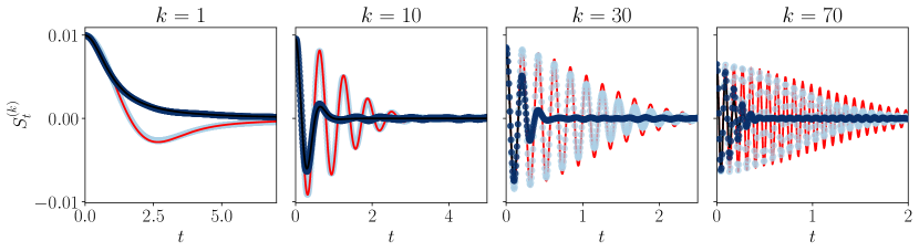
Figure 9: $k$-th neighbor Spectral Form Factor for the disordered XXZ spin chain for different neighbor levels $k=1,10,30,70$ in the chaotic ($W=1$, light blue dots) and the integrable ($W=20$, dark blue dots) phases along with the Poissonian (black line) and GOE (red line) curves. The deviation between the integrable phase and the Poissonian results is apparent starting from $k=10$, and increases for larger $k$. Note that the oscillations differ only in their amplitude but not in their frequency. We emphasis the different scales in the time axis.

IV.4 Dynamical signatures of chaos ($k$nSFF) in the disordered XXZ

To test how the dynamical signatures of a real system match those of idealized models, we extract data for the $k$nSFF from the XXZ model with disorder. Figure 9 shows numerical results for the $k$th neighbor SFF for various values of $k$, where the behavior for a disorder strength of $W=1$ can be compared with $W=20$. It shows how the spin chain differs from the Poissonian ensemble with increasing spectral distance $k$, due to reminiscent spectral correlations.

Figure 1 shows results for the minimum value of $S^{(k)}_{t}$ as a function of $k$ as well as the values of $k^{*}$ as a function of the disorder strength $W$. In particular, $k^{*}$ exhibits a transition, similar to that probed by $\langle r\rangle$, as coded in the colorscale. The values of $k^{*}$ at the two ends of the range of $W$, which correspond to integrable (large $W$) and chaotic (small $W$), are exactly those predicted from the Poissonian and GOE ensembles respectively, for the window size we used to extract the data (compare with Figure 8). Similarly to the spectral statistics, the dynamical signature also deviates from the results expected from the Poissonian ensemble as $k$ becomes large. Nevertheless, we are not expecting to see a ‘ramp’ since the ramp is mainly influenced by the behavior of $S^{(k)}_{t}$ at small $k$. Indeed, the full SFF shown in Figure 17 does not exhibit a ramp or even a ‘correlation hole’ in the case of large disorder. The works [32, 33] consistently find no ‘correlation hole’ for large disorder in this model.

IV.5 Summing it up: the complete SFF

We now add up the contributions from all spectral distance to write the total SFF, and compare our approximate analytical results to numerical simulations. Using the approximations (65) for the $k$th neighbor SFF, the total averaged SFF for the Gaussian ensembles is given approximately by:

$$S_{t}\approx\frac{1}{N}+\sum_{k=1}^{N-1} \frac{2(N-k)}{N^{2}}e^{-\frac{\omega_{k}^{2}t^{2}}{4\alpha}}\Big{[}\cos(\omega_{k}t)$$ (76)

$$+\frac{1}{12\alpha}\omega_{k}t\Big{(}\frac{\omega_{k}^{2}t^{2}}{2\alpha}-3\Big{)}\sin(\omega_{k}t)\Big{]}.$$

Figure 10 presents the results for the integrable and chaotic models. It shows that for the Gaussian ensembles, the above approximate expression gives good results, even without using any exact results for $S_{t}^{(k)}$. In particular, the transition between the ramp and plateau is well captured for the three ensembles: smooth for GOE, ‘kink’ for GUE and ‘spike’ for GSE. The time at which this transition happens was first discussed in [14] and we provide an alternative rational for it by decomposing the SFF into the contributions from odd and even spectral distances, see below. Importantly, all the ensembles, when properly unfolded, show the plateau time at $t_{p}=2\pi$. In Appendix H, we test the accuracy of the total result given in Eq. (76).

One question which naturally arises from the discussion below Eq. (63) is: how important is the contribution of the sines? Can we recover the full SFF from just summing over the cosine part? i.e. with a Gaussian approximation for the $k$nLS distribution. The answer is that we get a correlation hole, but no linear ramp, and that the sines contributions are especially important at the beginning of the ramp and at the transition to the plateau.

Figure 10: Spectral Form Factor for: Poisson (black), GOE (red), GUE (green) and GSE (blue) computed numerically (thick transparent line) and using the analytical results (thin solid line) given by (77) (black) and (76) (red, green, blue). The plots show results for random matrices with dimension $N=100$ and the numerics have been averaged over $N_{\mathrm{av}}=1000$ matrices. The dotted line marks the start of the plateau at $t_{p}=2\pi$. The behavior of the SFF for the different RM ensembles can be understood from the even and odd level contributions, as discussed in the main text.

The total averaged SFF for the Poissonian ensemble is given exactly by

$$S_{t}^{(\text{Poisson})}=\frac{1}{N}+\sum_{k=1}^{N-1}\frac{2(N-k)}{N^{2}}\frac{\cos(k\arctan t)}{(1+t^{2})^{k/2}}.$$ (77)

Although for $k>1$ the $k$th neighbor SFF for the Poissonian ensemble has a dip and shows some oscillations before flattening out (as can be seen in Figure 6), the full Poissonian SFF has no ‘dip’ or ‘correlation hole’, as expected for completely uncorrelated levels.

Figure 11: Odd vs even neighbor contributions to the SFF and their sum for Poisson, GOE, GUE and GSE; computed numerically from $N_{\mathrm{av}}=1000$ matrices of dimension $N=100$. For visualization of the data in log-log scale, an extra factor of $1/2N$ was added to the even and odd contributions. The vertical lines highlight the time at which the anti-resonance happens, $t^{*}=\pi$ (dashed gray), and at which the plateau starts for RMT, $t_{p}=2\pi$ (dotted gray).

Even and odd contributions.— The approximation (65) for the ensemble average of the $k$th component of the RMT SFF is expressed as a combination of cosines and sines with frequency $\omega_{k}$ given by (63). Figure 11 presents the numerical results for the even and odd level contributions, defined as

$$\langle\mathcal{S}_{t}^{(\text{even})}\rangle \equiv\frac{1}{2N}+\sum_{k\;\mathrm{even}}\langle\mathcal{S}_{t}^{(k)}\rangle$$ (78a)

$$\langle\mathcal{S}_{t}^{(\text{odd})}\rangle \equiv\frac{1}{2N}+\sum_{k\;\mathrm{odd}}\langle\mathcal{S}_{t}^{(k)}\rangle,$$ (78b)

for random matrices taken from GOE, GUE and GSE ensembles of dimension $N=100$. Inspecting the plots, we find a constructive interference for $\langle\mathcal{S}_{t}^{(\text{even,odd})}\rangle$ at $t\approx\pi$. More specifically, there is a “resonance” for $\langle\mathcal{S}_{t}^{(\text{even})}\rangle$ and an “anti-resonance” for $\langle\mathcal{S}_{t}^{(\text{odd})}\rangle$ at $t\approx\pi$. This observation can be explained by our analytical results,

$$S_{t}^{(\text{even})} \approx\frac{1}{2N}+\sum_{k\text{ even}}C_{N}^{(k)}f_{t}^{(k)}$$ (79a)

$$S_{t}^{(\text{odd})} \approx\frac{1}{2N}+\sum_{k\text{ odd}}C_{N}^{(k)}f_{t}^{(k)},$$ (79b)

where $C_{N}^{(k)}$ is given by (47b) and $f_{t}^{(k)}$ is given by the approximation (IV.2). Taking $\omega_{k}\approx k$, the sum (79a) involves a sum of $\cos(k\,t)$ with $k=2,4,6,\dots$ which interfere constructively at $t=\pi$ to create a “peak” or a “resonance”; similarly, the sum (79b) involves a sum of $\cos(k\,t)$ with $k=1,3,5,\dots$ which interfere constructively at $t=\pi$ to create a “dip” or an “anti-resonance”. We also note that the ‘spike’ seen in the complete SFF for GSE (as can be seen in figure 10) is nothing but the next constructive interference from both the even and odd contributions, and happens (for the unfolded spectrum) at $t=2\pi$. Note that the transition from the ramp to the plateau also happens at $t_{p}=2\pi$ for GUE and at a similar time for GOE. This is consistent with the results in [14] which show the plateau for the Gaussian ensembles at $t_{p}/(2\pi\bar{\rho})=1$, in our case unfolding the spectra sets $\bar{\rho}=1$ and thus $t_{p}=2\pi$.

Figure 12: (a) $k$nSFF for GSE for $k=1,\;40,\;90$ (solid thin lines) and Gaussian envelope (dashed thick line), standard deviation of the Gaussian envelope $\sqrt{2\alpha}/\omega_{k}$ (solid horizontal lines) and plateau time $t_{p}=2\pi$ (dotted gray line). (b) Ratio between the plateau time $t_{p}=2\pi$ and the width of the Gaussian envelope $\sqrt{2\alpha}/\omega_{k}$ as a function of the neighbor degree $k$ for the three Gaussian ensembles: GOE (red), GUE (green) and GSE (blue).

Note that the fact that the GSE exhibits a spike is related to the Gaussian attenuation that multiplies the sum of cosines and sines in (76), which has a largest width in this ensemble. Indeed, the width is set by $\sqrt{\alpha}$, which is proportional to $\sqrt{\beta}$, as per its definition in Eq. (2), and the GSE has the largest $\beta$ (equal to 4). Fig. 12 shows the ratio of the plateau time $t_{p}=2\pi$ to the width of the Gaussian envelope for GOE, GUE and GSE. The envelope width is the largest for the GSE, in which the plateau time lies between 2 and 3 standard deviations of the Gaussian envelope.

IV.6 The complete SFF with only nearest-neighbor correlations

As we have shown extensively in this article, the nearest-neighbor level spacing, although indicative of chaotic or regular behavior, is not a sufficient condition for chaos, since truly chaotic models (as modeled by RM) have correlations all over the spectrum. In this spirit, we construct a toy model which only has energy correlations to nearest neighbors, but nowhere else in the spectrum. What would be the SFF of such a system? To answer this, let us recall that the probability distribution of the sum of two uncorrelated random variables $z=x+y$ is given by their convolution. So, in this toy model, the second level spacing distribution simply reads

$$\mathcal{P}^{(2)}(s^{(2)}) =\mathcal{P}^{(1)}(s^{(1)})*\mathcal{P}^{(1)}(s^{(1)})$$ (80)

$$=\int_{0}^{s^{(2)}}\mathrm{d}s\mathcal{P}^{(1)}(s)\mathcal{P}^{(1)}(s^{(2)}-s).$$

The convolution theorem states that the Fourier transform of a convolution is the product of the Fourier transform, and vice versa. The $k$nSFF for this toy model follows as

$$S^{(k)}_{t}=\mathrm{Re}(\mathcal{F}[\mathcal{P}^{(1)}]^{k}(t)),$$ (81)

where the Fourier transform of the nnLS distribution, $\mathcal{F}[\mathcal{P}^{(1)}](t)$, admits the exact expression

$$\mathcal{F}[\mathcal{P}^{(1)}](t)= \>{}_{1}F_{1}\left(\frac{\beta+1}{2},\frac{1}{2},-\frac{t^{2}}{4A_{\beta}}\right)$$ (82)

$$-it\;{}_{1}F_{1}\left(\frac{\beta}{2}+1,\frac{3}{2},-\frac{t^{2}}{4A_{\beta}}\right).$$

Figure 13: SFF computed numerically for the GUE (green) and for the toy model with energy correlations to nearest neighbors only (purple), eq. (82).

The sum of the $k$nSFF is shown in Fig. 13 for the GUE ensemble. The SFF of this toy model shows a correlation hole, since it decays and grows back, but the ramp is not linear and therefore there is no chaos. Similar non-linear ramps in the SFF have been reported for integrable models like the SYK₂ [62, 63]. Thus, we conclude that correlations beyond nearest energy levels are needed to find the linear ramp in the SFF characteristic of chaotic systems.

V A dissipative protocol to measure the $k$nSFF

The autocorrelation function of a general operator $\hat{O}$ (48) can be obtained from knowledge of the spectrum and the operator. We propose a protocol, based on dissipative dynamics, to measure the $k$-neighbor autocorrelation function, introduced in (49).

Assuming that we are able to prepare an initial operator with non-zero weight only in its main and $k$-th diagonal, namely $\hat{O}^{(k)}=\sum_{n=1}^{N}O_{ii}\ket{i}\bra{i}+\sum_{i=1}^{N-k}O_{i+k,i}\ket{i+k}\bra{i}+\textrm{h.c.}$. Its autocorrelation function will be related to the $k$nSFF since it only contains spectral information from the $k$nLS,

$$\mathcal{C}_{t}^{(k)} =\frac{1}{\mathcal{N}^{2}}\mathrm{Tr}(\hat{O}^{(k)}\hat{O}_{t}^{(k)})$$ (83)

$$=\sum_{i}\frac{|O_{ii}|^{2}}{\mathcal{N}^{2}}+\sum_{i=1}^{N-k}\frac{|O_{i+k,i}|^{2}}{\mathcal{N}^{2}}\cos[(E_{k+i}-E_{i})t)].$$

If at this point we further assume that we unfold the spectrum, so that the $k$nLS $E_{i+k}-E_{i}$ does not depend on the density of states $\rho(E_{i})$, and average over a suitable ensemble, we find that the time evolution (49) will depend on time only through $f_{t}^{(k)}$, which in turn completely determines the $k$nSFF.

The initial operator $\hat{O}^{(k)}$ might look somewhat artificial, so let us propose a way to engineer it through a dissipative evolution. In the case of dissipative dynamics in which the unitary part is dictated by $\hat{H}_{0}$ and the dissipator consists of a single Hermitian jump operator $\hat{L}=\hat{L}^{\dagger}$, any system operator evolves according to the adjoint Lindblad equation [64, 65]

$$d_{t}\hat{O}_{t}=\mathrm{i}[\hat{H}_{0},\hat{O}_{t}]-\gamma\big{[}\hat{L},[\hat{L},\hat{O}_{t}]\big{]},$$ (84)

where $\gamma$ is the dissipation rate associated with $\hat{L}$. Considering commuting operators, $[\hat{H}_{0},\hat{L}]=0$, which then share a common eigenbasis, $\hat{H}=\sum_{i}E_{i}\ket{i}\bra{i},\;\hat{L}=\sum_{i}l_{i}\ket{i}\bra{i}$, the solution of the above equation simply reads

$$\hat{O}_{t}=\sum_{i,j}O_{ij}e^{-\mathrm{i}(E_{i}-E_{j})t-\gamma(l_{i}-l_{j})^{2}t}\ket{i}\bra{j}.$$ (85)

We now assume that we do not apply the Hamiltonian dynamics yet (e.g going to a rotating frame such that they are not relevant) and that we can engineer the jump operator in a way such that its eigenvalues repeat once after the $k$-th element, namely

$$\hat{L}=\mathrm{diag}(l_{1},\dots,l_{k},l_{1},\dots,l_{k},l_{2k+2},\dots,l_{N}),$$ (86)

where we have set $l_{k+i}=l_{i}$ for $1\leq i\leq k$, and we also consider no extra degeneracies $l_{i}\neq l_{j}$ $\forall\;i,j\in\{1,\dots,k,2k+2,\dots N\}$. The evolution at a time $T$ becomes $\hat{O}_{T}=\sum_{i,j}O_{ij}e^{-\gamma(l_{i}-l_{j})^{2}T}\ket{i}\bra{j}$. All off-diagonal elements decay exponentially fast with time, except for those with $|i-j|=k$ and $i,j\in\{1,\dots,k\}$ which are preserved due to the structure of $\hat{L}$. Thus we see that $\lim_{T\rightarrow\infty}\hat{O}_{T}=\hat{O}^{(k)}=\sum_{i=1}^{N}\hat{O}_{ii}\ket{i}\bra{i}+\sum_{i=1}^{2k}O_{i+k,i}\ket{i+k}\bra{i}+\mathrm{h.c.}$, i.e. this protocol leads to a matrix with $2k$ nonzero elements only in the $k$-th diagonal. The full diagonal could be optained by repeating the the sequence of eigenvalues $l_{1},\dots,l_{k}$ more times in (86), but this would lead to higher “harmonics”, i.e. nonzero terms for $|i-j|=2k,3k,\dots$, which would contain contributions from higher degree $k$nSFF’s.

Other possible experimental probes are to experimentally measure the energy levels of the system, compute the $k$nLS distribution and the associated $k$nSFF by a Fourier transform. Alternatively, another way could be to use the partial SFF introduced in [22]. More specifically, one would need to find a partition the total Hilbert space in two, $\mathscr{H}=\mathscr{H}_{A}\otimes\mathscr{H}_{B}$, such that the condition $\mathrm{Tr}_{B}(\rho_{B}(E_{i})\rho_{B}(E_{j}))\propto\delta_{|i-j|,k}$ holds, where $\rho_{B}(E_{i})=\mathrm{Tr}_{A}(\ket{E_{i}}\bra{E_{i}})$. If there exists such a subspace $\mathscr{H}_{A}$, then the randomized measurement protocol devised in [22] could be readily used to compute the $k$nSFF’s and $k$nLS distribution.

VI Summary and discussion

In this work, we introduced measures of spectral correlations at all-ranges in the spectrum, yielding new refined probes of quantum chaos. Our model for chaotic systems are random matrices taken from the three Gaussian ensembles, GOE, GUE and GSE, and our basic model for integrable systems is the ensemble of completely uncorrelated energy levels (Poissonian ensemble) with uniform density of states. Real systems, as illustrated by the disordered XXZ spin chain, have spectral properties that lie in-between these ensembles around the densest parts of their spectrum.

While works in the literature usually focus on nearest-neighbor spectral statistics (spacings or ratios) or on the properties of the spectral form factor which probes all energy levels at once, we chose to study all-range spectral statistics (within an energy window located around the densest part of the spectrum) by “decomposing” the spectrum according to sets of spacings with increasing distances. Specifically, we focused on full-range spectral statistics in the form of the $k$th neighbor level spacing probability distribution and on the resulting $k$th neighbor spectral form factor. For the $k$nLS distributions, we introduced its variance as a probe that distinguishes chaos from integrability, with significantly different behaviors, and the Poissonian value $1/k$ for the normalized splittings $\tilde{s}$ acting as an upper bound on the possible width of any $\mathcal{P}^{(k)}(\tilde{s})$ of a spectrum with correlated levels. We note here that the $k$nLS distributions can also be used to find the eigenvalue distribution of the Liouvillian superoperator, which consists of all energy differences, as we discuss in Appendix I. They also relate to the large $N$ sine-kernel, see Appendix J.

Taking a Fourier transform of the $k$nLS distributions, we found expressions for the $k$th neighbor SFFs for the random matrix ensembles and for the Poissonian ensemble. By applying a few approximations, we could express the RMT $k$nSFF as a sum of cosines and sines with appropriate polynomial coefficients and an overall Gaussian envelope function. This realization of the $k$nSFF provides insight into the transition between the ramp and plateau for the different Gaussian ensembles. From studying the $k$nSFFs, we found that their minimum value as a function of $k$ is markedly different between chaotic and integrable systems. Thus, the ‘deepest’ $k$nSFF contributing to the full SFF and the corresponding energy distance $k^{*}$ as a function of $N$ provides a refined probe of quantum chaos. In a similar spirit, we defined the $k$th neighbor decomposition of the autocorrelation function for operators.

We tested our analytical results and approximations against numerical data extracted from many realizations of the random matrices in the various ensembles we studied (Poissonian, GOE, GUE and GSE) and found good agreement. We then checked how closely a real system follows the trends we found for the idealized random matrix and Poisson ensembles. The XXZ model with disorder interpolates between GOE statistics and Poissonian statistics as the disorder strength increases. As expected from the Bohigas-Giannoni-Schmit and Berry-Tabor conjectures, the chaotic phase shows correlations similar to those of GOE, while the integrable phase shows Poissonian statistics. With our refined probes of all-range spectral correlations, specifically the variance of the $k$nLS, we were able to witness small deviations from the expected RMT statistics, especially relevant at large $k$. Also, we were able to attribute the deviation from the integrable model to persistent correlations when the level spacing increases.

For the Gaussian ensembles, the several approximations we made to achieve simple, tractable expressions capture the main properties of the complete SFF, as verified against numerical simulations. Our results show that the ramp feature found in the SFF of chaotic systems is a result of intricate relationships between $k$nSFF’s of increasing spectral distances $k$. Specifically, the nearest-neighbor level repulsion only is not enough to induce a ramp. Also, the specific shape of the set of $\mathcal{P}^{(k)}(\tilde{s})$ and, in particular, the strong suppression at small $\tilde{s}$ are important in achieving the specific features of the $k$nSFF which eventually build up the complete SFF. In particular, if the $k$nLS probability distributions were perfectly Gaussian, the results for the $k$nSFF would involve only a Gaussian envelope and a cosine term. Such a structure would not give rise to the specific features of the complete SFF, particularly around the transition from the ramp to the plateau. Hence, the non-Gaussianity of the $k$nLS distributions is crucial to capture the full chaotic signature of the SFF. We probe the non-Gaussianity of these distributions through the skewness and kutorsis in Appendix D. We further discuss the self-averaging properties of the individual $k$nSFFs in Appendix E.

This work opens many new directions for future study; we mention some below. We have made several approximations in our derivation of the $k$th neighbor level spacing distributions. While they capture the main behavior, we expect corrections at large $k$, and it would be interesting to study their effect on the $k$nSFFs and the full SFF in future work. Some other possible directions are to study how finite temperature affects the $k$nSFF’s [24], or to extend the $k$nLS and $k$nSFF’s to the dissipative case, where mostly only nearest-neighbor correlations and SFF’s have been studied [66, 67]. We only began investigating how far the correlations between energy levels should persist in finding a linear ramp in the full SFF. We leave to future research the investigation of the $k$th neighbor autocorrelation functions we defined in this work. In particular, they can be used to understand better the behavior of the autocorrelation function for different operators. Lastly, one other possible extension of our results is in the field of log-gases [56]. In this context, the $k$nLS distribution $\mathcal{P}^{(k)}(s)$ gives the strength of interaction between a particle and its $k$-th neighbor, re-summing all the interactions with all the other particles.

To summarize, our results suggest that to investigate quantum chaos fully, it is important to include in our analysis correlations at any range since the correlations beyond first energy neighbors have a clear manifestation in dynamical quantities such as the spectral form factor, and will also show up in time-dependent correlation functions. The specific nature of the level repulsion at longer range distances rather than just nearest-neighbor repulsion plays an important role in accurately capturing the details of such dynamical quantities at all time scales.

Appendix A Numerical implementation of the Gaussian ensembles

In this appendix we review the definitions and numerical manifestations of the three Gaussian random matrix ensembles: GOE, GUE and GSE.

GOE: We sample a $N\times N$ random matrix $X$ with entries given from a real normal distribution with $\sigma=1$, i.e.

$$X_{ij}=\mathcal{N}(0,1),\quad 1\leq i,j\leq N.$$

Matrices from GOE are symmetric, therefore $H\in\mathrm{GOE}(N)$ is given by

$$H=\frac{1}{2}(X+X^{T}).$$

GUE: Matrices from GUE are Hermitian, so their elements are generated from complex numbers, i.e.

$$X_{ij}=\mathcal{N}(0,1)+i\mathcal{N}(0,1),\quad 1\leq i,j\leq N.$$

From $X$, we can generate a Hermitian matrix simply by

$$H=\frac{1}{2}(X+X^{\dagger}),\quad H\in\mathrm{GUE}(N).$$

GSE: Generating matrices from the symplectic ensemble is slightly more involved. We need to generate a matrix $X$ of dimension $2N$

$$X_{ij}=\mathcal{N}(0,1)+i\mathcal{N}(0,1),\quad 1\leq i,j\leq 2N,$$

and introduce the skew Hermitian matrix $J$ defined as

$$J=\left(\begin{array}[]{cc}0&-1\\ 1&0\end{array}\right)\otimes\mathbb{1}_{N}.$$

Then, an element of the $\mathrm{GSE}(N)$ is given by

$$H=\frac{1}{2\sqrt{2}}\left(X+X^{\dagger}-J(X+X^{\dagger})^{T}J\right).$$

Appendix B Details of proof for $k$th neighbor level spacing distribution

This appendix provides the explicit forms of $\mathbf{A}$ and $\mathbf{B}$ which appear in the quadratic polynomial $\overline{q}(\{x_{i}\}_{i=1}^{k-1})$.

The quadratic polynomial $q(\{x_{i}\}_{i=1}^{k})$ written in (22), once restricted by $x_{k}=1-\sum_{i=1}^{k-1}x_{i}$, takes the form

$$\overline{q}(\{x_{i}\}_{i=1}^{k-1})=\frac{k}{k+1}-2\sum_{i=1}^{k-1}\frac{k-i}{k+1}x_{i}$$ (87)

$$+\sum_{i=1}^{k-1}\frac{(k-i)(i+1)}{k+1}x_{i}^{2}+2\sum_{i<j=1}^{k-1}\frac{(k-j)(i+1)}{k+1}x_{i}x_{j}~{}.$$

From here, we can read off the elements $B_{i}$ and $A_{ij}$ for $i,j=1,\dots,k-1$ as

$$B_{i} =\frac{k-i}{k+1},$$ (88)

$$A_{ii} =\frac{(k-i)(i+1)}{k+1},$$ (89)

$$A_{i\neq j} =\frac{(k-\max(i,j))(\min(i,j)+1)}{k+1}~{}.$$ (90)

It can be checked that $\mathbf{A}$ is positive definite. The inverse of $\mathbf{A}$ is a tridiagonal, almost Toeplitz matrix , with diagonal $A^{-1}_{11}=3/2$ and $A^{-1}_{ii}=2$ for $i\neq 1$, and off-diagonals $A^{-1}_{i,i+1}=A^{-1}_{i-1,i}=-1$. Also, it can be verified that $\mathbf{m}=\mathbf{A}^{-1}\mathbf{B}=(1/2,0,0,\dots,0)$.

Appendix C Unfolding the spectrum

The spectrum of a system is a property which a priori depends on the system under consideration. However, its energy correlations can obey some universal laws. To study the latter, we need to remove the dependence on the spectrum on non-universal features, like the density of states $\bar{\rho}(E)$, to get a universal spectrum completely given by its correlations. In doing so, systems that are originally completely different can be compared. The procedure to obtain such a universal spectrum is known as unfolding (see e.g. [9]). In this appendix, we explain how we unfold a generic spectrum. We then study some aspects of the effect of unfolding on our results.

Our method of unfolding involves computing the function

$$f(E)=N\int_{-\infty}^{E}dE^{\prime}\,\bar{\rho}(E^{\prime})~{}.$$ (91)

where $\bar{\rho}(E)$ is the average density of states, and then pass the energy eigenvalues $\{E_{i}\}_{i=1}^{N}$ into this function to get the set of unfolded energy levels $\{e_{i}\}_{i=1}^{N}=\{f(E_{i})\}_{i=1}^{N}$. For the random matrix ensembles we study, the average density of states is given by the Wigner semicircle distribution, $\bar{\rho}(E)=\frac{1}{\pi\beta N}\sqrt{2N\beta-E^{2}}$. This leads to an analytical form for the function $f(E)$, which reads

$$f(E)=\frac{N}{2}+\frac{1}{\pi\beta}\left(N\beta\arcsin\ \frac{E}{\sqrt{2N\beta}}+\frac{E}{2}\sqrt{2N\beta-E^{2}}\right),$$ (92)

for $-\sqrt{2\beta N}<E<\sqrt{2\beta N}$, while it is $f(E)=0$ for $E\leq-\sqrt{2\beta N}$ and $f(E)=N$ for $E\geq\sqrt{2\beta N}$, see also [70].

For the disordered XXZ spin chain, there is no analytical expression for the average density of states. We thus rely on a numerical polynomial fit for $f(E)$ for each realization of disorder. We used a larger window of energies to perform the fit, and then discarded the two edges, thus focusing our analysis on a window of around $N=200$ energies.

Our numerical unfolding depends on two parameters: the maximum order of the polynomial fit $\eta$ and the number of bins with which we construct our histogram (related to the bin’s width). These parameters, especially the polynomial order, can critically change the results since we can be over-fitting the spectrum and include some of the universal correlations into the density of states. To check which minimum order gives a reasonable fit, we compare the numerical and analytical unfolding on a random matrix and define a quality of the fit, $\mathcal{Q}$, as the square of the difference between the histograms of the analytical and numerical unfolded spectra, namely

$$\mathcal{Q}=\sum_{n\in\mathrm{bins}}\left(\mathrm{Hist}_{n}(f^{\mathrm{ana}}(E))-\mathrm{Hist}_{n}(f^{\mathrm{num}}(E))\right)^{2}.$$ (93)

Figure 14 shows that $\eta=3$ is an unfolding order with already good results. So, we chose this order to avoid over-fitting. The parameter of the number of bins is not too critical, and we set $N_{\mathrm{bins}}=50$ to have enough bins and enough points per bin.

Figure 14: Quality of the unfolding as a function of the order and the number of bins for the GOE.

Although our results refer to the unfolded spectrum, we study here some of the same results for the folded (i.e. the original, not unfolded spectrum), namely, the dip times for the $k$nSFFs and the even-odd signatures discussed in Section IV.5. We also compare the total folded vs unfolded SFF for disorder XXZ spin chain at two values of the disorder parameter $W$ representative of the integrable and chaotic phases.

As can be seen in Figure 15, the dip times for the folded $k$nSFFs of the Gaussian ensembles no longer follow the relation $t_{d}\approx\pi/k$ perfectly. However, they still follow a $t_{d}(k)\sim k^{-1}$ decay with small corrections.

Figure 15: Dip time as a function of the neighbor degree for: Poisson (black), GOE (red), GUE (green) and GSE (blue) computed numerically from the folded spectrum along with an $t_{d}(k)\sim k^{-1}$ dependence (dashed gray).

Another interesting aspect of unfolded versus folded results is whether the even-odd signatures, described in Section IV.5, are still present without unfolding. Figure 16 confirms that such a signature is still present. The main difference is in the time at which the ‘resonance’ and ‘anti-resonance’ appear: while for the unfolded spectrum, they appear at $t=\pi$, for the folded spectrum, they appear at a time scale related to the matrix dimension.

Figure 16: The even- (red) and odd- (blue) neighbor contributions are compared for the folded and unfolded cases of Poisson, GOE, GUE, and GSE. The black solid line is the total SFF. The figure shows numerical data from random matrices of dimension $N=100$ averaged over $N_{\textrm{av}}=1000$ realizations.

For completeness, we compare the unfolded with the folded results for the total SFF of disordered XXZ spin-chain at two values of $W$, see Figure 17.

Figure 17: Spectral Form Factor using the unfolded (up) or folded (down) spectrum of the XXZ spin chain with disorder strengths $W=1$ (left) and $W=20$ (right). The unfolded results (top) are compared with the RMT results (left, red dash-dotted) and the Poisson ensemble (right, black dash-dotted). The parameters are $L=10$, $N_{\uparrow}=5$, $J=1,\;J_{z}=2,\;N_{\mathrm{av}}=200$.

Appendix D How good is the Gaussian approximation for the $k$nLS distribution?

Figure 18: Skewness and kurtosis for: GOE (red), GUE (green) and GSE (blue) computed from the asymptotic power laws (solid lines) and numerically (circles) for matrices of dimension $N=100$. The numerical results use $N_{\mathrm{av}}=10^{5}$ realizations of the ensemble. (insets) Skewness and Kurtosis in log-log scale, also show Poisson results (black). The value of $k=N/2$ (dotted gray line).

As discussed in the main text, the non-Gaussianity of the $k$nLS distributions is important for recovering the specific features of the total SFF. The non-Gaussianity of a distribution can be measured through quantities such as the skewness, characterizing the asymmetry of the distribution, and the kurtosis, characterizing the tailed-ness of the distribution. They are defined as

$$\mathrm{Skew}^{(k)} =\mathbb{E}\left[\left(\frac{s^{(k)}-\mu}{\sigma}\right)^{3}\right],$$ (94)

$$\mathrm{Kurt}^{(k)} =\mathbb{E}\left[\left(\frac{s^{(k)}-\mu}{\sigma}\right)^{4}\right],$$ (95)

where $\mathbb{E}[\bullet]=\int_{0}^{\infty}\mathcal{P}(s)\bullet\mathrm{d}s$ is the expectation value, $\mu$ is the mean and $\sigma$ is the standard deviation of the distribution. Using the generalized Wigner distribution, $\mathcal{P}^{(k)}(s)=C_{\alpha}s^{\alpha}e^{-A_{\alpha}s^{2}}$ as in Eq. (1), we find

$$\mathrm{Skew}_{\beta}^{(k)} =\frac{\sqrt{2}\left(4\Gamma\left(\frac{\alpha}{2}+1\right)^{3}-(2\alpha+1)\Gamma\left(\frac{\alpha}{2}+1\right)\Gamma\left(\frac{\alpha+1}{2}\right)^{2}\right)}{\left((\alpha+1)\Gamma\left(\frac{\alpha+1}{2}\right)^{2}-2\Gamma\left(\frac{\alpha}{2}+1\right)^{2}\right)^{3/2}},$$ (96)

$$\mathrm{Kurt}_{\beta}^{(k)} =\frac{-12\Gamma\left(\frac{\alpha}{2}+1\right)^{4}+(\alpha+1)(\alpha+3)\Gamma\left(\frac{\alpha+1}{2}\right)^{4}+\pi 4^{1-\alpha}(\alpha-1)\Gamma(\alpha+1)^{2}}{\left((\alpha+1)\Gamma\left(\frac{\alpha+1}{2}\right)^{2}-2\Gamma\left(\frac{\alpha}{2}+1\right)^{2}\right)^{2}}.$$ (97)

In turn, the distribution from the Poissonian ensemble (5) yields

$$\mathrm{Skew}_{0}^{(k)}=\frac{2}{\sqrt{k}},\textrm{ and }\quad\mathrm{Kurt}_{0}^{(k)}=3+\frac{6}{k}.$$ (98)

The expressions for RMT admit the asymptotic expansions

$$\mathrm{Skew}_{\beta}^{(k)}=\frac{1}{\sqrt{2\alpha}}+\mathcal{O}(\alpha^{-3/2}),\quad\mathrm{Kurt}_{\beta}^{(k)}=3+\frac{3}{4\alpha^{2}}+\mathcal{O}(\alpha^{-3}),$$ (99)

which show that both the (excess) kurtosis and the skewness go to zero faster as a function of $k$ in RMT than in Poisson. In other words, as we increase $k$, the generalized Wigner distribution approaches a Gaussian distribution faster than the Poisson results do. Figure 18 shows the comparison with numerical random matrices. We see that a real random matrix has a skewness that follows the derived power-law for small $k$, but starts decaying faster until it changes sign at $k=N/2$, i.e. the distribution after this point becomes asymmetric with a tail to the right. Interestingly, the skewness for $k\sim N$ looks opposite to the one for small $k$, which suggests that the function is antisymmetric around $k=N/2$. The kurtosis for random matrices, however, behaves very differently from the derived power laws, from which we conclude that the tails of the $k$nLS distribution are not well captured by the generalized Wigner surmise.

Appendix E Self-averaging of the $k$th neighbor SFF

In this appendix we discuss the self-averaging properties of the $k$th neighbor SFFs, as a function of $k$.

A quantity is said to be self averaging if its relative variance becomes smaller as the system size is increased. The SFF is known to be particularly not self-averaging around its plateau (the flat part which the SFF tends to at large $t$), i.e. the relative variance of its plateau increases as $N$ is increased. Here, we numerically study the self averaging of the plateau of the $k$th neighbor SFF. The relative variance of the $k$th neighbor SFF can be defined as (see e.g. [33]):

$$R_{k}(t)=\frac{\langle(\mathcal{S}_{t}^{(k)}+\bar{\mathcal{S}})^{2}\rangle-\langle\mathcal{S}_{t}^{(k)}+\bar{\mathcal{S}}\rangle^{2}}{\langle\mathcal{S}_{t}^{(k)}+\bar{\mathcal{S}}\rangle^{2}}~{},$$ (100)

where $\bar{\mathcal{S}}=\tfrac{1}{N(N-1)}$ is the value of the plateau divided equally among the $N-1$ possible neighbors, which we added such that the average $\langle\mathcal{S}_{t}^{(k)}+\bar{\mathcal{S}}\rangle$ is non-zero.

Figure 19 shows the relative variance of the plateau as a function of the neighbor degree $k$ for different dimensions of the random matrices. We can observe several features:

• $\mathcal{S}^{(k)}_{t}$ is never self averaging since the relative variance increases with the dimension of the matrix.

• The limiting value of the relative variance decreases linearly with $k$ in the following way

  $$\bar{R}_{k}^{\mathrm{plat}}=\frac{1}{T}\int_{t_{p}}^{t_{p}+T}R_{k}(\tau)d\tau=(N-k)\frac{N-1}{2N},$$ (101)

  where indeed Figure 19 suggests a linear function of $k$ with a constant slope independent of $N$ and a constant which scales linearly with $N$.

Figure 19: Relative variance of the plateau of the $k$nSFF as a function of the neighbor degree $k$, for GUE random matrices of dimension $N$ (colorscale). The results are averaged over $N_{\mathrm{av}}=1000$ ensemble realizations and $\bar{R}^{\mathrm{plat}}_{k}:=\frac{1}{T}\int_{t_{p}}^{t_{p}+T}R_{k}(\tau)d\tau$ is the time averaged relative variance on the plateau. Solid lines correspond to (101).

Appendix F Details on the $k$-th dip time

To complete the discussion of the dip time in Section IV.2, Fig. 20 compares the approximation (66) against the numerical dip times computed from the exact (56) and the approximate (65) analytical results. We see that (66) is a very good approximation of the dip time for $k\geq 2$ and for $k=1$, although there is a small dependence on $\beta$ in the exact result, (66) is a better approximation than the dip time computed from (65). We therefore confirm our conclusion that the dip time of the $k$nSFF shows almost no dependence on the ensemble $\beta$.

Figure 20: Dip time as a function of neighbor-degree $k$ for: GOE (red), GUE (green) and GSE (blue) as computed numerically from: exact expression (56) (circles), approximation of $k$nSFF (65) (crosses) and approximation of $t_{d}(k)$ (66) (dotted line). The inset highlights the deviations for close neighbors in energy $k=1,2,3$. The approximation (66) cancels some errors and gives a better estimate to the full analytics (56) than the values computed from (65)

Appendix G The $k$th neighbor autocorrelation functions

In this appendix, we complete some of the steps leading to the result (49) in Section IV.1.

Figure 21: Difference between numerical and approximate analytical SFF for: Poisson, GOE, GUE and GSE. Dashed line marks $25\%$ difference between the numerics and the analytics.

Consider the infinite-temperature operator autocorrelation function for a Hermitian operator $O$ (i.e. an observable):

$$C_{t}\equiv\frac{\mathrm{Tr}(O^{\dagger}O(t))}{\mathrm{Tr}(O^{\dagger}O)}{=}\frac{1}{\mathcal{N}^{2}}\sum_{i,j=1}^{N}|O_{ij}|^{2}\cos(E_{i}-E_{i})t,$$

where $O_{ij}$ are the matrix elements of the operator $O$ in the energy basis and $\mathcal{N}^{2}=\sum_{i,j=1}^{N}|O_{ij}|^{2}$. This expression can be decomposed according to level-spacing distances, as follows

$$\mathcal{C}_{t} = \frac{1}{\mathcal{N}^{2}}\sum_{i=1}^{N}|O_{ii}|^{2}$$

$$+ \frac{2}{\mathcal{N}^{2}}\sum_{k=1}^{N-1}\sum_{i=1}^{N-k}|O_{i,i+k}|^{2}\cos(ts_{i}^{(k)}).$$

Performing an ensemble-average over the spectrum, which taken as unfolded ($E_{i+k}-E_{i}$ does not depend on $\rho(E_{i})$) so that $\mathcal{P}^{(k)}(s)$ can be used, the ensemble-averaged $C_{t}$ can be re-written as

$$C_{t}=\frac{1}{\mathcal{N}^{2}}\sum_{i=1}^{N}|O_{ii}|^{2}+\sum_{k=1}^{N-1}C^{(k)}_{t},$$ (103)

where we defined the $k$th neighbor autocorrelation function

$$C_{t}^{(k)}\equiv O_{N}^{(k)}\,f_{t}^{(k)}~{},$$ (104)

with $f_{t}^{(k)}$ defined in (47a) and with the coefficients

$$O_{N}^{(k)}\equiv\frac{2}{\mathcal{N}^{2}}\sum_{i=1}^{N-k}|O_{i,i+k}|^{2}~{}.$$ (105)

Appendix H Test of the approximations for the SFF

Since we have made several approximations on the way to our final expressions for the total SFF for the Gaussian ensembles, (76), we test the validity of our approximate analytical expression. Figure 21 shows the relative error between the exact SFF (computed from numerical data) and the expression (76) for the three Gaussian ensembles, as well as a comparison between the Poissonian expression (77) and numerical data for the SFF taken from the Poissonian ensemble. We see that in GOE and GUE the approximation over-estimates slightly the ramp, and specially in GOE has a distance to it of around 25% of the value of the SFF at that point.

Appendix I Distribution of eigenvalues of the Liouvillian

The distributions $\mathcal{P}^{(k)}(s)$ are strongly related to the eigenvalue distribution of the Liouvillian, as we explain in this appendix.

In the case of unitary dynamics, the Liouvillian superoperator is defined as

$$\mathcal{L}(\bullet)\equiv[\hat{H},\bullet],$$ (106)

in terms of the energies $E_{n}$ and eigenvectors $\ket{n}$ of $\hat{H}$ the Liouvillian has the eigendecomposition $\mathcal{L}(\ket{n}\bra{m})=(E_{n}-E_{m})\ket{n}\bra{m}$, i.e. the eigenvalues of the Liouvillian are all the energy differences $\lambda_{nm}=E_{n}-E_{m}$. The probability density of $\lambda_{nm}$ for $n\neq m$ then is the sum of all the $k$nLS distributions [13]

$$\mathcal{P}(\lambda)=\frac{2}{N(N-1)}\sum_{k=1}^{N-1}(N-k)\mathcal{P}^{(k)}(\lambda).$$ (107)

This sum is shown in Fig. 22 where the RMT ensembles show the expected level repulsion around $\lambda=0$, the Poisson ensemble shows initially a linear decay with $\mathcal{P}_{\beta}(\lambda)\sim-\lambda$. After the initial growth due to level repulsion GUE and GSE show oscillations, peaked at $\lambda=k\in\mathbb{N}$, with the oscillations being more pronounced in GSE.

Figure 22: Distribution of eigenvalues of Liouvillian computed from the analytical expressions with $N=10$ for: Poisson (black), GOE (red), GUE (green) and GSE (blue).

Appendix J $k$nLS distribution versus Sine Kernel

Figure 23: $\mathcal{P}^{(k)}(s)$ distribution for GUE for the first 12 neighbors (green lines), along with sine kernel $1-\mathrm{sinc}^{2}(\pi s)$ (orange) and sum of the distributions (green dashed lines).

Many studies of the GUE use a convenient large $N$ result known as the sine-kernel which leads to several nice analytic expressions [14, 15, 17, 16]. For completeness, we discuss how to get the sine-kernel from our $k$nLS distributions. We begin by introducing the 2-point spectral connected correlation function $\rho_{c}(E,E^{\prime})$ of a certain ensemble as [54]

$$\rho_{c}(E,E^{\prime})=\left\langle\rho(E)\rho(E^{\prime})\right\rangle-\langle\rho(E)\rangle\langle\rho(E^{\prime})\rangle,$$ (108)

where $\rho(E)=\sum_{j}\delta(E-E_{j})$ and thus $\langle\rho(E)\rangle$ is the density of states of an ensemble. After unfolding, i.e. introducing the rescaled energies $\varepsilon=EN\langle\rho(E)\rangle$, the renormalized 2-point correlation reads

$$\frac{\rho_{c}(E,E^{\prime})}{\langle\rho(E)\rangle\langle\rho(E^{\prime})\rangle}=\delta(\varepsilon-\varepsilon^{\prime})-Y(\varepsilon,\varepsilon^{\prime}),$$ (109)

where $Y(\varepsilon,\varepsilon^{\prime})$ is Dyson’s two-level cluster function, defined as

$$Y(\varepsilon,\varepsilon^{\prime})=1-\left\langle\sum_{m\neq n}\delta(\varepsilon-\varepsilon_{n})\delta(\varepsilon^{\prime}-\varepsilon_{m})\right\rangle.$$ (110)

This function depends only on the difference $s=\varepsilon-\varepsilon^{\prime}$ and for the GUE in the large $N$ limit reads [54]

$$Y^{\textsc{gue}}(s)=\mathrm{sinc}^{2}(\pi s),$$ (111)

where the sinc function is defined as $\mathrm{sinc}(x)=\sin(x)/x$. Therefore, for the GUE, we find that

$$\left\langle\sum_{m\neq n}\delta(\varepsilon-\varepsilon_{n})\delta(\varepsilon^{\prime}-\varepsilon_{m})\right\rangle=1-\mathrm{sinc}^{2}(\pi s).$$ (112)

Figure 23 compares the sum of the $k$nLS distributions with the expression for the sine kernel, noting that they give similar results, and therefore the sum in the l.h.s. of (112) is related to the sum of the $k$nLS distributions $\sum_{k=1}^{N-1}\mathcal{P}^{(k)}(s)$.

References

- Wigner [1956] E. P. Wigner, Results and theory of resonance absorption, Conference on Neutron Physics by Time of Flight (1956), p. 59.
- Wigner [1951] E. P. Wigner, On the statistical distribution of the widths and spacings of nuclear resonance levels, Mathematical Proceedings of the Cambridge Philosophical Society 47, 790–798 (1951).
- Gaudin [1961] M. Gaudin, Sur la loi limite de l’espacement des valeurs propres d’une matrice aléatoire, Nuclear Physics 25, 447 (1961).
- Wigner [1967] E. P. Wigner, Random matrices in physics, SIAM Review 9, 1 (1967).
- Garg et al. [1964] J. B. Garg, J. Rainwater, J. S. Petersen, and W. W. Havens, Neutron resonance spectroscopy. III. Th232 and U238, Phys. Rev. 134, B985 (1964).
- Bohigas et al. [1984] O. Bohigas, M. J. Giannoni, and C. Schmit, Characterization of Chaotic Quantum Spectra and Universality of Level Fluctuation Laws, Physical Review Letters 52, 1 (1984).
- Berry and Tabor [1977] M. V. Berry and M. Tabor, Level clustering in the regular spectrum, Proceedings of the Royal Society of London. A. Mathematical and Physical Sciences 356, 375 (1977).
- Mehta [2004] M. L. Mehta, Random matrices (Elsevier, 2004).
- Guhr et al. [1998] T. Guhr, A. Muller-Groeling, and H. A. Weidenmuller, Random matrix theories in quantum physics: Common concepts, Phys. Rept. 299, 189 (1998).
- Wimberger [2014] S. Wimberger, Nonlinear dynamics and quantum chaos, Vol. 10 (Springer, 2014).
- Srivastava et al. [2018] S. C. Srivastava, A. Lakshminarayan, S. Tomsovic, and A. Bäcker, Ordered level spacing probability densities, Journal of Physics A: Mathematical and Theoretical 52, 025101 (2018).
- Leviandier et al. [1986] L. Leviandier, M. Lombardi, R. Jost, and J. P. Pique, Fourier Transform: A Tool to Measure Statistical Level Properties in Very Complex Spectra, Physical Review Letters 56, 2449 (1986).
- Wilkie and Brumer [1991] J. Wilkie and P. Brumer, Time-dependent manifestations of quantum chaos, Physical Review Letters 67, 1185 (1991).
- Alhassid and Levine [1992] Y. Alhassid and R. D. Levine, Spectral autocorrelation function in the statistical theory of energy levels, Physical Review A 46, 4650 (1992).
- Ma [1995] J.-Z. Ma, Correlation Hole of Survival Probability and Level Statistics, Journal of the Physical Society of Japan 64, 4059 (1995).
- Cotler et al. [2017a] J. S. Cotler, G. Gur-Ari, M. Hanada, J. Polchinski, P. Saad, S. H. Shenker, D. Stanford, A. Streicher, and M. Tezuka, Black holes and random matrices, Journal of High Energy Physics 2017, 118 (2017a).
- Cotler et al. [2017b] J. Cotler, N. Hunter-Jones, J. Liu, and B. Yoshida, Chaos, complexity, and random matrices, Journal of High Energy Physics 2017, 48 (2017b).
- del Campo et al. [2017] A. del Campo, J. Molina-Vilaplana, and J. Sonner, Scrambling the spectral form factor: Unitarity constraints and exact results, Physical Review D 95, 126008 (2017).
- Chenu et al. [2019] A. Chenu, J. Molina-Vilaplana, and A. del Campo, Work Statistics, Loschmidt Echo and Information Scrambling in Chaotic Quantum Systems, Quantum 3, 127 (2019).
- Chenu et al. [2018] A. Chenu, I. L. Egusquiza, J. Molina-Vilaplana, and A. del Campo, Quantum work statistics, Loschmidt echo and information scrambling, Scientific Reports 8, 12634 (2018).
- Vasilyev et al. [2020] D. V. Vasilyev, A. Grankin, M. A. Baranov, L. M. Sieberer, and P. Zoller, Monitoring Quantum Simulators via Quantum Nondemolition Couplings to Atomic Clock Qubits, PRX Quantum 1, 020302 (2020).
- Joshi et al. [2022] L. K. Joshi, A. Elben, A. Vikram, B. Vermersch, V. Galitski, and P. Zoller, Probing Many-Body Quantum Chaos with Quantum Simulators, Physical Review X 12, 011018 (2022).
- Prange [1997] R. E. Prange, The Spectral Form Factor Is Not Self-Averaging, Physical Review Letters 78, 2280 (1997).
- Martinez-Azcona and Chenu [2022] P. Martinez-Azcona and A. Chenu, Analyticity constraints bound the decay of the spectral form factor, Quantum 6, 852 (2022).
- Vikram and Galitski [2022] A. Vikram and V. Galitski, Exact universal bounds on quantum dynamics and fast scrambling (2022), arXiv:2212.14021 .
- Žnidarič et al. [2008] M. Žnidarič, T. Prosen, and P. Prelovšek, Many-body localization in the heisenberg x x z magnet in a random field, Physical Review B 77, 064426 (2008).
- Pal and Huse [2010] A. Pal and D. A. Huse, Many-body localization phase transition, Physical Review B 82, 174411 (2010).
- Serbyn and Moore [2016] M. Serbyn and J. E. Moore, Spectral statistics across the many-body localization transition, Physical Review B 93, 041424 (2016).
- Bertrand and García-García [2016] C. L. Bertrand and A. M. García-García, Anomalous thouless energy and critical statistics on the metallic side of the many-body localization transition, Physical Review B 94, 144201 (2016).
- Sierant and Zakrzewski [2019] P. Sierant and J. Zakrzewski, Level statistics across the many-body localization transition, Physical Review B 99, 104205 (2019).
- Šuntajs et al. [2020] J. Šuntajs, J. Bonča, T. Prosen, and L. Vidmar, Quantum chaos challenges many-body localization, Physical Review E 102, 062144 (2020).
- Schiulaz et al. [2019] M. Schiulaz, E. J. Torres-Herrera, and L. F. Santos, Thouless and relaxation time scales in many-body quantum systems, Physical Review B 99, 174313 (2019).
- Schiulaz et al. [2020] M. Schiulaz, E. J. Torres-Herrera, F. Pérez-Bernal, and L. F. Santos, Self-averaging in many-body quantum systems out of equilibrium: Chaotic systems, Physical Review B 101, 174312 (2020).
- Bekenstein [2008] J. Bekenstein, Bekenstein-Hawking entropy, Scholarpedia 3, 7375 (2008).
- Maldacena [2003] J. M. Maldacena, Eternal black holes in anti-de Sitter, JHEP 04, 021.
- Kitaev [2015a] A. Kitaev, Hidden correlations in the Hawking radiation and thermal noise, KITP seminar (2015a).
- Kitaev [2015b] A. Kitaev, A simple model of quantum holography, KITP strings seminar and Entanglement (2015b).
- Maldacena et al. [2016] J. Maldacena, S. H. Shenker, and D. Stanford, A bound on chaos, Journal of High Energy Physics 2016, 106 (2016).
- Almheiri et al. [2021] A. Almheiri, T. Hartman, J. Maldacena, E. Shaghoulian, and A. Tajdini, The entropy of Hawking radiation, Rev. Mod. Phys. 93, 035002 (2021).
- Maldacena and Stanford [2016] J. Maldacena and D. Stanford, Remarks on the Sachdev-Ye-Kitaev model, Phys. Rev. D 94, 106002 (2016).
- Rao [2020] W.-J. Rao, Higher-order level spacings in random matrix theory based on Wigner’s conjecture, Physical Review B 102, 054202 (2020).
- Engel et al. [1998] D. Engel, J. Main, and G. Wunner, Higher-order energy level spacing distributions in the transition region between regularity and chaos, Journal of Physics A: Mathematical and General 31, 6965 (1998).
- Abul-Magd and Simbel [1999] A. Y. Abul-Magd and M. H. Simbel, Wigner surmise for high-order level spacing distributions of chaotic systems, Physical Review E 60, 5371 (1999).
- Tekur et al. [2018] S. H. Tekur, U. T. Bhosale, and M. S. Santhanam, Higher-order spacing ratios in random matrix theory and complex quantum systems, Physical Review B 98, 104305 (2018).
- Sakhr and Nieminen [2006] J. Sakhr and J. M. Nieminen, Wigner surmises and the two-dimensional homogeneous Poisson point process, Physical Review E 73, 047202 (2006).
- Forrester [2009] P. J. Forrester, A Random Matrix Decimation Procedure Relating = 2/(r + 1) to = 2(r + 1), Communications in Mathematical Physics 285, 653 (2009).
- Note [1] We will omit the superscript when it is clear that we are discussing the th level spacings.
- Oganesyan and Huse [2007] V. Oganesyan and D. A. Huse, Localization of interacting fermions at high temperature, Physical Review B 75, 155111 (2007).
- Atas et al. [2013] Y. Atas, E. Bogomolny, O. Giraud, and G. Roux, Distribution of the ratio of consecutive level spacings in random matrix ensembles, Physical review letters 110, 084101 (2013).
- Bethe [1931] H. Bethe, Zur theorie der metalle: I. eigenwerte und eigenfunktionen der linearen atomkette, Zeitschrift für Physik 71, 205 (1931).
- Kawabata et al. [2023] K. Kawabata, A. Kulkarni, J. Li, T. Numasawa, and S. Ryu, Symmetry of open quantum systems: Classification of dissipative quantum chaos, PRX Quantum 4, 030328 (2023).
- Kahn and Porter [1963] P. B. Kahn and C. E. Porter, Statistical fluctuations of energy levels: The unitary ensemble, Nuclear Physics 48, 385 (1963).
- Abul-Magd and Simbel [2000] A. Y. Abul-Magd and M. H. Simbel, High-order level-spacing distributions for mixed systems, Physical Review E 62, 4792 (2000).
- Haake [1991] F. Haake, Quantum signatures of chaos (Springer, 1991).
- Berry and Shukla [2018] M. V. Berry and P. Shukla, Geometric phase curvature for random states, Journal of Physics A: Mathematical and Theoretical 51, 475101 (2018).
- Forrester [2010] P. J. Forrester, Log-Gases and Random Matrices (LMS-34), in Log-Gases and Random Matrices (LMS-34) (Princeton University Press, 2010).
- Dyson [1962] F. J. Dyson, Statistical Theory of the Energy Levels of Complex Systems. I, Journal of Mathematical Physics 3, 140 (1962).
- Note [2] We expect such a behavior for an unfolded spectrum ( does not depend on the local density of states ) which shows no mixed behavior, i.e. the spectral statistics does not change within the energy window.
- Mirevski and Boyadjiev [2010] S. Mirevski and L. Boyadjiev, On some fractional generalizations of the laguerre polynomials and the kummer function, Computers & Mathematics with Applications 59, 1271 (2010).
- Note [3] See Digital Library of Mathematical Functions https://dlmf.nist.gov/18.15##iv.
- Note [4] Note that we are not expanding terms involving time in .
- Winer et al. [2020] M. Winer, S.-K. Jian, and B. Swingle, An exponential ramp in the quadratic Sachdev-Ye-Kitaev model, Physical Review Letters 125, 250602 (2020).
- Liao et al. [2020] Y. Liao, A. Vikram, and V. Galitski, Many-body level statistics of single-particle quantum chaos, Physical Review Letters 125, 250601 (2020).
- Breuer and Petruccione [2002] H.-P. Breuer and F. Petruccione, The theory of open quantum systems (Oxford University Press on Demand, 2002).
- Rivas and Huelga [2012] A. Rivas and S. F. Huelga, Open quantum systems, Vol. 10 (Springer, 2012).
- Sá et al. [2020] L. Sá, P. Ribeiro, and T. Prosen, Complex Spacing Ratios: A Signature of Dissipative Quantum Chaos, Physical Review X 10, 021019 (2020).
- Xu et al. [2019] Z. Xu, L. P. García-Pintos, A. Chenu, and A. del Campo, Extreme Decoherence and Quantum Chaos, Physical Review Letters 122, 014103 (2019).
- Note [5] Further properties of Toeplitz matrices can be found in https://mathworld.wolfram.com/ToeplitzMatrix.html.
- Note [6] This result can be found in https://robertsweeneyblanco.github.io/Computational_Random_Matrix_Theory/Eigenvalues/Wigner_Surmise.html.
- Abul-Magd and Abul-Magd [2014] A. A. Abul-Magd and A. Y. Abul-Magd, Unfolding of the spectrum for chaotic and mixed systems, Physica A: Statistical Mechanics and its Applications 396, 185 (2014).