Kagome Materials II: SG 191: FeGe as a LEGO Building Block for the Entire 1:6:6 series: hidden d-orbital decoupling of flat band sectors, effective models and interaction Hamiltonians

Abstract

The electronic structure and interactions of kagome materials such as 1:1 (FeGe class) and 1:6:6 (MgFe₆Ge₆ class) are complicated and involve many orbitals and bands at the Fermi level. Current theoretical models treat the systems in an $s$-orbital kagome representation, unsuited and incorrect both quantitatively and qualitatively to the material realities. In this work, we lay the basis of a faithful framework of the electronic model for this large class of materials. We show that the complicated “spaghetti” of electronic bands near the Fermi level can be decomposed into three groups of $d$-Fe orbitals coupled to specific Ge orbitals. Such decomposition allows for a clear analytical understanding (leading to different results than the simple $s$-orbital kagome models) of the flat bands in the system based on the $S$-matrix formalism of generalized bipartite lattices. Our three minimal Hamiltonians can reproduce the quasi-flat bands, van Hove singularities, topology, and Dirac points close to the Fermi level, which we prove by extensive ab initio studies. We also obtain the interacting Hamiltonian of $d$ orbitals in FeGe using the constraint random phase approximation (cRPA) method. We then use this as a fundamental “LEGO”-like building block for a large family of 1:6:6 kagome materials, which can be obtained by doubling and perturbing the FeGe Hamiltonian. We applied the model to its kagome siblings FeSn and CoSn, and also MgFe₆Ge₆. Our work serves as the first complete framework for the study of the interacting phase diagram of kagome compounds.

Introduction. Kagome materials exhibit a rich phase diagram including charge density waves Chen et al. (2022); Diego et al. (2021); Ferrari et al. (2022); Kenney et al. (2021); Li et al. (2021a, 2023); Liang et al. (2021); Liu et al. (2021a); Luo et al. (2022); Kiesel et al. (2013); Ratcliff et al. (2021); Song et al. (2021a); Setty et al. (2021); Tan et al. (2021); Tsirlin et al. (2022); Tsvelik and Sarkar (2023); Uykur et al. (2021, 2022); Wang et al. (2021a, b, c); Yu et al. (2021a); Zhu et al. (2022); Zhao et al. (2021); Guo et al. (2023); Lin and Nandkishore (2021), superconductivity Ortiz et al. (2020); Chen et al. (2021a, b); Du et al. (2021); Duan et al. (2021); Feng et al. (2021); Kang et al. (2023a); Li et al. (2022); Liu et al. (2021b); Mu et al. (2021); Nakayama et al. (2021); Ni et al. (2021); Shrestha et al. (2022); Song et al. (2021b); Wang et al. (2021d, e, 2023); Wu et al. (2021); Xiang et al. (2021); Xu et al. (2021a); Yin et al. (2021a, b); Yu et al. (2021b); Zhang et al. (2022a), different magnetic ordersTeng et al. (2022); Mazet et al. (2013); Häggström et al. (1975a); Ishikawa et al. (2021); Li et al. (2021b); Liu et al. (2023); Pal et al. (2022); Ye et al. (2018) and topological statesGuo and Franz (2009); Bolens and Nagaosa (2019); Yin et al. (2022a); Hu et al. (2022); Liu et al. (2019, 2018); Xu et al. (2018). In recent years, kagome superconductors AV₃Sb₅ (A=K, Cs, and Rb)Ortiz et al. (2019); Cho et al. (2021); Kang et al. (2021); Ortiz et al. (2021a, b); Kautzsch et al. (2023) of the 1:3:5 class with unusual charge ordersDenner et al. (2021); Neupert et al. (2022); Jiang et al. (2021); Mielke et al. (2022); Shumiya et al. (2021); Wang et al. (2021f); Guo et al. (2022); Wagner et al. (2023) but no soft phonon modes observedLi et al. (2021c); Xie et al. (2022); Liu et al. (2022); Subires et al. (2023), and ScV6Sn6 Arachchige et al. (2022); Korshunov et al. (2023); Hu et al. (2023a); Cao et al. (2023); Cheng et al. (2023); Kang et al. (2023b); Tan and Yan (2023); Hu et al. (2023b); Lee et al. (2023); Tuniz et al. (2023); Yi et al. (2023); Hu et al. (2023c); Gu et al. (2023); Guguchia et al. (2023); Cheng et al. (2023); Mozaffari et al. (2023) of the 1:6:6 class Venturini (2006); Fredrickson et al. (2008); Venturini et al. (2008); Mazet et al. (2013) with soft phonon modes first observed in experimentsKorshunov et al. (2023); Cao et al. (2023) have attracted much attention. Among the kagome materials, the kagome magnet FeGeTeng et al. (2022, 2023); Miao et al. (2022); Setty et al. (2022); Yin et al. (2022b); Zhou et al. (2023); Chen et al. (2023a); Ma et al. (2023); Wang (2023); Wu et al. (2023a); Chen et al. (2023b, c); Wu et al. (2023b, c); Zhang et al. (2023); Zhao et al. (2023); Shi et al. (2023) of the 1:1 class (or, equivalently, 3:3 class) is particularly attractive: it develops an A-type antiferromagnetic (AFM) order below $T_{N}=410$ $K$Ohoyama et al. (1963); Häggström et al. (1975b); Forsyth et al. (1978), and, more interestingly, has a CDW transition at $T_{\text{CDW}}=100$ $K$Teng et al. (2022, 2023). The kagome 1:1 class materials in SG 191 have formula TZ, where T are transition metals and Z are the main group elements. The 1:6:6 class, however, has the formula MT₆Z₆ where M are metallic elements, which can be seen as doubled 1:1 materials (which is T3Z3) with inserted $M$ atoms.

A commonly used theoretical model for understanding the non-trivial phase diagram of kagome systems is the $s$-orbital tight-binding (TB) model with nearest-neighbor hoppings on a kagome latticeMielke (1991). However, such an $s$-orbital TB model is incorrect for FeGe. It is oversimplified and fails to give quantitative descriptions for realistic kagome materials, which have a large number of orbitals near the Fermi level that are entangled together. However the model also suffers a qualitative fault: the Z element sits at the trigonal and honeycomb sites around the kagome T element can hop to it. This type of model in general should not have flat bands.

In this work, for the first time, we are able to provide a clear and comprehensive understanding of the complicated “spaghetti” of electronic bands for the kagome 1:1 and 1:6:6 materials. Our strategy is to decompose the intricate band structures into several small groups where, within each group, a simple and analytical understanding of the band structures is feasible. We first consider the 1:1 class and take FeGe as a representative. We separate the $d$ orbitals of Fe into three groups that are combined with specific orbitals of Ge based on chemical and symmetry analyses. Three decoupled effective tight-binding models for three groups can then be constructed, where the effective tight-binding models not only quantitatively reproduce the quasi-flat bands, van Hove singularities (vHS), and Dirac points, but also provide an analytical understanding of the origin of flat bands, which are only flat on part of the BZ. Moreover, we also provide the full interacting Hamiltonian and identify a hidden $O_{h}$ symmetry of the interacting term. We then move on to the 1:6:6 family MT₆Z₆. Remarkably, the Hamiltonian of the 1:6:6 family can be obtained by doubling and perturbing the 1:1 Hamiltonian. We thus treat FeGe as a “LEGO”-like building block and successfully construct the band structures of 1:6:6 material MgFe₆Ge₆Mazet et al. (2013).

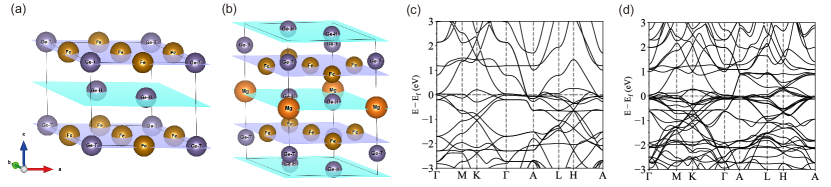
Figure 1: (a) Crystal structure of FeGe, where Fe atoms form a kagome lattice, and Ge atoms form a trigonal lattice (denoted by Ge-T in the plot) and a honeycomb lattices (denoted by Ge-H). (b) Crystal structure of MgFe6Ge6, which can be seen as a doubled FeGe along $z$-direction and inserting Mg atoms in the middle plane of honeycomb Ge. (c)(d): Band structure of FeGe and MgFe6Ge6 in the paramagnetic phase, respectively.

Decomposition of orbitals. We now introduce the main idea: build minimal effective models that reproduce the complicated band structure of 1:1 and 1:6:6 classes near the Fermi level $E_{f}$ by decomposing the orbitals into independent groups.

We start from the atomic positions in SG 191 $P6/mmm$, which can be divided into three sublattices, i.e., trigonal, honeycomb, and kagome, depending on their site symmetry groups. On a two-dimensional (2D) plane with basis $\bm{a}_{1}=(1,0),\bm{a}_{2}=(-\frac{1}{2},\frac{\sqrt{3}}{2})$, trigonal lattice has Wyckoff position $1a=(0,0)$ with $C_{6z}$ symmetry, honeycomb lattice has $2b=(\frac{1}{3},\frac{2}{3}),(\frac{2}{3}$, $\frac{1}{3})$ with $C_{3z}$, while kagome lattice has $3c=(\frac{1}{2},0)$, $(\frac{1}{2},\frac{1}{2})$, $(0,\frac{1}{2})$ with $C_{2z}$. In 3D systems, atoms can occupy these three sublattices on different $z$ planes. For example, in 1:1 materials like FeGe, three Fe atoms occupy the kagome lattice on the $z=0$ plane, one Ge atom occupies the trigonal lattice on $z=0$ plane (denoted by Ge^T) and the other two Ge on the honeycomb lattice on $z=\frac{1}{2}$ plane (denoted by Ge^H), as shown in Fig. 1(a). The 1:6:6 materials MT6Z6 can be seen as a doubled unit cell of the corresponding 1:1 material T3Z3 with M atoms inserted on the trigonal lattice on one layer of the honeycomb lattice, with MgFe6Ge6 as an example shown in Fig. 1(b). We remark that there also exist more complicated superstructures in the 1:6:6 class that are built from multiple 1:1 materialsVenturini et al. (2008), all of which can be understood from the 1:1 family using perturbation theory.

The orbitals decompose into three groups. In 1:1 materials, the $d$ orbitals of the kagome lattice contribute most to the bands close to $E_{f}$. We first decompose the five kagome $d$ orbitals into three groups of $(d_{xy},d_{x^{2}-y^{2}})$, $(d_{xz},d_{yz})$, and $d_{z^{2}}$, and then couple each of them with specific orbitals from trigonal and honeycomb lattices that have dominant hoppings. The kagome $d$ orbitals, when combined with orbitals from trigonal and honeycomb lattices, form generalized bipartite crystalline lattices (BCL) and the $S$-matrix formalismCălugăru et al. (2022); Regnault et al. (2022) can be readily applied to identify the perfectly flat band limits. We emphasize that such decomposition holds for generic 1:1 material TZ, since T are transition metals that usually provide $d$ orbitals and Z are the main group elements that usually provide $s,p$ orbitals. We apply this strategy to 1:1 materials including FeGe, FeSnHäggström et al. (1975a); Sales et al. (2019); Multer et al. (2022), and CoSnLarsson et al. (1996). With the effective model constructed for 1:1 materials, the model for 1:6:6 materials can be derived by doubling that of the corresponding 1:1 materials and treating the orbitals of M atoms as a perturbation. MgFe6Ge6 is used as a representative example in this work.

Band structure of FeGe and MgFe6Ge6. We first consider FeGe in the 1:1 class and use density functional theory (DFT)Kresse and Furthmüller (1996a); Kresse and Hafner (1993a, b, 1994); Kresse and Furthmüller (1996b) to compute band structures as a starting point for constructing effective models. The bands in the PM phases of FeGe are shown in Fig. 1(c) (for the AFM phase, see Appendix I). This spaghetti-like band structure is very complicated and hosts two quasi-flat bands connected with other bands and multiple vHSs near $E_{f}$. For 1:6:6 class representative MgFe6Ge6, the even more complicated band structure is shown in Fig. 1(d). However, one can observe that the bands of MgFe6Ge6 are very close to that of FeGe by folding the bands on $k_{z}=0$ and $\pi$ planes together to the $k_{z}=0$ plane of MgFe6Ge6, which results from the fact that MgFe6Ge6 is doubled FeGe along $z$-direction with extra Mg atoms. This observation inspires us to construct effective Hamiltonians of 1:6:6 class from 1:1 class.

Three minimal effective Hamiltonians. We first construct maximally localized Wannier functions (MLWFs)Marzari and Vanderbilt (1997); Souza et al. (2001); Marzari et al. (2012) and obtain a Wannier TB model, and perform a detailed study of orbital projections, density of states, and orbital fillings using MLWFs for each $d$ orbitals  (see Section II.1). The TB model obtained from MLWFs, although faithful, still contains more than 20 orbitals and a huge number of hopping parameters. It is desirable to build minimal TB Hamiltonians that can not only reproduce the band structure but also help gain insight into the physical properties of the system, including the origin of the quasi-flat bands near $E_{f}$. However, it is not straightforward to see how to simplify the system with such a large number of degrees of freedom. Here, based on symmetry and chemical analysis, we divide the orbitals into three groups and construct TB models for them separately, as shown in Fig. 2.

First, the five $d$ orbitals of Fe split into three groups under $D_{6h}$ (which is the point group of SG 191), i.e., $(d_{xy},d_{x^{2}-y^{2}})$, $(d_{xz},d_{yz})$, and $d_{z^{2}}$. The inplane hopping between $(d_{xz},d_{yz})$ and the other three $d$ orbitals are forbidden by $M_{z}$ symmetry as they have opposite $M_{z}$ eigenvalues, and $z$-directional hoppings are weak and can be neglected. The hoppings between $(d_{xy},d_{x^{2}-y^{2}})$ and $d_{z^{2}}$, although not negligible and not forbidden by symmetry, are small compared with other leading hopping terms and will be neglected as an approximation. We then combine the three groups of $d$ orbitals with specific orbitals of Ge based on both chemical and symmetry analysis, as shown in Fig. 2: (i) $d_{xy},d_{x^{2}-y^{2}}$ of Fe and $p_{x},p_{y}$ of Ge^T. These orbitals lie on the $z=0$ plane and have large overlaps, forming $\sigma$-like bonds, which can be verified from the Wannier hoppings. They form a BCL of eight bands, and the $S$-matrix formalismCălugăru et al. (2022); Regnault et al. (2022) can be applied to identify the perfect flat band limit when the hoppings take specific forms (to be discussed in the next paragraph). (ii) $d_{xz},d_{yz}$ of Fe and $p_{z}$ orbitals of both Ge^T and Ge^H. These orbitals all lie along the $z$-direction and have large overlaps, forming $\pi$-like bonds, verified from the Wannier hoppings. (iii) $d_{z^{2}}$ orbitals of Fe and the $sp^{2}$ bonding state formed by the $s,p_{x}$ and $p_{y}$ orbitals of honeycomb Ge (equivalent to an $s$ orbital on kagome lattice of $z=\frac{1}{2}$ plane).

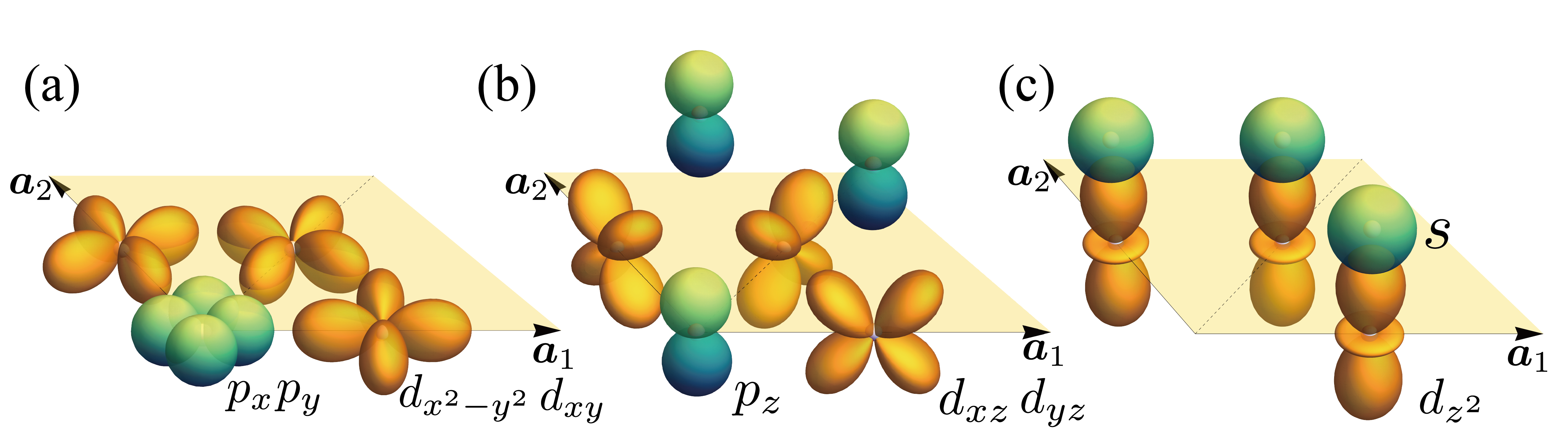
Figure 2: Decomposition of three sets of orbitals. (a) $d_{x^{2}-y^{2}},d_{xy}$ of kagome Fe and $p_{x},p_{y}$ of trigonal Sn ($d_{x^{2}-y^{2}}$ is shown and $d_{xy}$ omitted in the plot for simplicity). (b) $d_{xz},d_{yz}$ of kagome Fe and $p_{z}$ of trigonal and honeycomb Sn ($d_{xz}$ is shown and $d_{yz}$ omitted for simplicity). (c) $d_{z^{2}}$ of kagome Fe and the bonding state (equivalent to $s$ orbital on $z=\frac{1}{2}$ plane) of honeycomb Sn. The yellow plane denotes the $z=0$ plane in the unit cell. A local coordinate system on kagome lattice that rotates with $C_{6z}$ is used (see Section II.1) s.t. five $d$ orbitals can be separated under SG 191 symmetries.

With three groups of orbitals, we then construct TB models $H_{i=1,2,3}(\bm{k})$ for them separately, with the total Hamiltonian being a direct sum:

$$H(\bm{k})=H_{1}(\bm{k})\oplus H_{2}(\bm{k})\oplus H_{3}(\bm{k}).$$ (1)

$H_{1}(k)$: $d_{xy},d_{x^{2}-y^{2}}$ of Fe and $p_{x},p_{y}$ of trigonal Ge.

These orbitals have elementary band representations (EBRs) $E_{1u}@1a$, $A_{g}@3f$, and $B_{1g}@3f$, corresponding to $(p_{x},p_{y})$, $d_{xy}$, and $d_{x^{2}-y^{2}}$, respectively (denoted as $p_{xy}^{t}$, $d_{1}$, and $d_{2}$). We construct a TB Hamiltonian of the form (see Section II.3.1 for the explicit form of each block):

$$H_{1}(\bm{k})=\left(\begin{matrix}H_{p_{xy}^{t}}(\bm{k})&S_{p_{xy}^{t},d_{1}}(\bm{k})&S_{p_{xy}^{t},d_{2}}(\bm{k})\\ &H_{d_{1}}(\bm{k})&S_{d_{1},d_{2}}(\bm{k})\\ h.c.&&H_{d_{2}}(\bm{k})\\ \end{matrix}\right).$$ (2)

We fit the TB parameters to DFT results by considering both dispersions and IRREPs at high-symmetry points, and the resultant band structure has similar quasi-flat bands at $E_{f}$. In DFT, the quasi-flat band at $E_{f}$ mainly comes from $d_{x^{2}-y^{2}}$, and we identify a perfect flat band limit in $H_{1}(\bm{k})$ as $S_{d_{1},d_{2}}(\bm{k})=\bm{0}$ and $H_{d_{2}}(\bm{k})=\mu_{d_{2}}\bm{1}_{3}$, which will lead to a flat band from $d_{x^{2}-y^{2}}$ according to the $S$-matrix formalismCălugăru et al. (2022). The vanishing hopping in $H_{d_{2}}(\bm{k})$ can be seen as a result of the cancellation of effective hoppings from orbitals not considered in $H_{1}(\bm{k})$ (see Section II.3.1). The final fitted parameters are close to this flat band limit, resulting in the quasi-flat band near $E_{f}$. The wavefunction of this quasi-flat band has a high overlap of about 97% with DFT wavefunction. The vHS at about $-0.5$ eV at $M$ is also well-fitted in the current model. Note that the current $H_{1}(\bm{k})$ has only inplane hoppings and is $k_{3}$-independent, which will be remedied in the combined model by first coupling with $p_{z}$ orbital of honeycomb Ge and then perturbing out the coupling term which introduces the $k_{3}$-dependence to $H_{1}(\bm{k})$.

$H_{2}(k)$: $d_{xz},d_{yz}$ of Fe and $p_{z}$ of Ge

These orbitals form four EBRs, i.e., $A_{2}^{\prime\prime}@2d$, $A_{2u}@1a$, $B_{2g}@3f$, and $B_{3g}@3f$, corresponding to $p_{z}^{h}$ of Ge^H, $p_{z}^{t}$ of Ge^T, $d_{xz}$, and $d_{yz}$ (denoted as $d_{3}$ and $d_{4}$), respectively. We construct the following TB Hamiltonian (see Section II.3.2 for more details of each block)

$$H_{2}(\bm{k})=\left(\begin{array}[]{cccc}H_{p_{z}^{h}}(\bm{k})&\bm{0}&\bm{0}&S_{p_{z}^{h},d_{4}}(\bm{k})\\ &H_{p_{z}^{t}}(\bm{k})&S_{p_{z}^{t},d_{3}}(\bm{k})&\bm{0}\\ &&H_{d_{3}}(\bm{k})&S_{d_{3},d_{4}}(\bm{k})\\ h.c.&&&H_{d_{4}}(\bm{k})\\ \end{array}\right).$$ (3)

The perfectly flat band limit of $H_{2}(\bm{k})$ can be achieved by setting $S_{d_{3},d_{4}}(\bm{k})=0$, and $H_{4}(\bm{k})$ with only NN hoppings. In this case, $d_{4}$ hosts one perfectly flat band near $E_{f}$. We also identify a special flat band limit where one flat band exists on $(k_{1},0,k_{3})$ plane (including $\Gamma$-$M$, $\Gamma$-$A$, and $A$-$L$ lines, and other symmetry-related planes), but dispersive in other regions of BZ. This flat band limit can be realized by requiring $d_{3}$ and $d_{4}$ to have the same onsite energy and only inplane NN hoppings which satisfy $-t_{d_{3}}^{NN}=t_{d_{4}}^{NN}=-t_{d_{3},d_{4}}^{NN}$, and the resultant flat band is an equal-weight superposition of $d_{3}$ and $d_{4}$. Such equal-weight decomposition also holds approximately in DFT band structures (see orbital projections in Section II.1). The fitted TB parameters in $H_{2}(\mathbf{k})$ are close to the second limit, with bands shown in Fig. 3((e). An extremely flat exists along $\Gamma$-$M$, $\Gamma$-$A$, and $A$-$L$ lines. The overlap of the flat band wavefunction between the fitted $H_{2}(\bm{k})$ and DFT is about $85\%$.

$H_{3}(k)$: $d_{z^{2}}$ and $sp^{2}$ bonding state of honeycomb Ge

The bonding states are coupled with $d_{z^{2}}$ in order to introduce $d_{z^{2}}$ weights below $-2$ eV and reproduce the DFT band structure more faithfully, as seen from the orbital projections of DFT in Fig. 3(c). However, if one is only interested in the low energy dispersions near $E_{f}$, it is more convenient to use $d_{z^{2}}$ only to build a simpler model, as the $d_{z^{2}}$ weights given by the coupling with the bonding states are mainly below $-2$ eV. We then constructed a model for $d_{z^{2}}$ only, i.e., $H_{3}(\mathbf{k})=H_{d_{5}}(\bm{k})$. The explicit form of $H_{d_{5}}(\mathbf{k})$ and fitted dispersions are left in Appendix [II]. We remark that if one uses this simplified model of $d_{z^{2}}$ only, the Coulomb interaction of $d_{z^{2}}$ also needs to be renormalized to smaller values, as the weight of $d_{z^{2}}$ near $E_{f}$ is reduced by the bonding state.

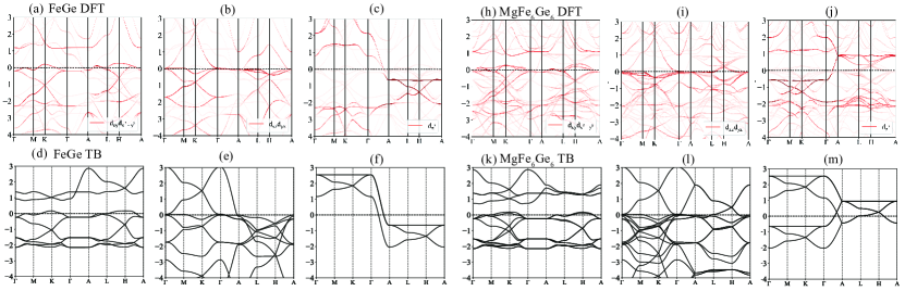
Figure 3: The DFT and TB band structures of FeGe and MgFe6Ge6. (a)-(c) The orbital projections of $(d_{xy},d_{x^{2}-y^{2}})$, $(d_{xz},d_{yz})$, and $d_{z^{2}}$, respectively, of DFT bands in FeGe. (d)-(f) The band structures of the three minimal TB Hamiltonian $H_{1}(\bm{k})$, $H_{2}(\bm{k})$, and $H_{3}(\bm{k})$ defined Eq. 4 for FeGe. (g)-(i) Same as (a)-(c), but for MgFe6Ge6. (j)-(l) Same as (d)-(f), but for MgFe6Ge6. The TB band structures of MgFe6Ge6 are obtained by folding the TB of FeGe along $k_{z}$ and treating the $s$ orbital of Mg as perturbations. The TB bands show a quantitative match with DFT bands near the Fermi level, and are more realistic compared with a single $s$-orbital kagome model, as our models give the correct orbital components for flat bands and capture the DFT dispersion trend in a wide energy range.

Combined model

We then combine the three $H_{i}(\bm{k})$ together and use second-order perturbation theory for further simplification and give the final model.

One extra coupling term $S_{p_{z}^{h},d_{2}}(\bm{k})$ between $d_{x^{2}-y^{2}}$ and $p_{z}$ of Ge^H is introduced to capture $k_{z}$-dispersion in $H_{1}(\mathbf{k})$ (see Section II.3.4). This term can be perturbed out as these two orbitals have relatively large onsite energy differences. Similar perturbation is also performed for $p_{z}^{t}$ in $H_{2}(\mathbf{k})$. The final Hamiltonian obtained is the direct sum of three models:

$$H(\bm{k})=H_{1}(\bm{k})\oplus H_{2}(\bm{k})\oplus H_{3}(\bm{k}),$$ (4)

in which $H_{d_{2}}(\bm{k})$, $H_{p_{z}^{h}}$, and $H_{d_{3}}$ are modified by second-order perturbation terms to $H_{d_{2}}(\bm{k})+H_{d_{2},p_{z}^{h}}^{(2)}(\bm{k})$, $H_{p_{z}^{h}}(\bm{k})+H_{p_{z}^{h},d_{2}}^{(2)}(\bm{k})$, and $H_{d_{3}}(\bm{k})+H_{d_{3},p_{z}^{t}}^{(2)}(\bm{k})$, respectively, with $H_{O_{1},O_{2}}^{(2)}$ denoting the hopping block of $O_{1}$ orbital that comes from the second-order perturbed term of $O_{2}$ orbitals (see Appendix VIII). The band structure of $H(\bm{k})$ is shown in Fig. 3(d)-(f), which quantitatively reproduces the quasi-flat bands, vHS, and Dirac points close to $E_{f}$ as in the dispersion of DFT. Mismatches of TB and DFT bands mainly appear at the energy about 1 $eV$ away from $E_{f}$, which are less relevant to low-energy physics in both PM and AFM phases. The vHSs in the three sectors are also well-fitted which will move close to $E_{f}$ in the AFM phase and could be important for the CDW formation. The mismatches arise because there are weights of other orbitals away from $E_{f}$ in DFT, which are not considered in our minimal TB model.

Interacting Hamiltonian from cRPA. With the minimal TB Hamiltonian, we then compute the Coulomb interaction using the constraint random phase approximation (cRPA) methodAryasetiawan et al. (2004); Solovyev and Imada (2005); Aryasetiawan et al. (2006); Miyake et al. (2009) (see Appendix III) to construct the interaction Hamiltonian. The onsite inter-orbital Hubbard $U_{m_{i},m_{j}}$, onsite exchange $J_{m_{i},m_{j}}$, and NN and NNN Hubbard $U_{m_{i},m_{j}}^{NN/NNN}$ are evaluated where $m_{i,j}$ are orbital indices. In Appendix III, we computed $U_{m_{i},m_{j}}$, $J_{m_{i},m_{j}}$, and $U_{m_{i},m_{j}}^{NN/NNN}$ for the so-called $d-dp$ model, $dp-dp$ modelVaugier et al. (2012), and $d$-full models, which are constructed using different sets of MLWFs with different spread. We observe that there is an approximate hidden symmetry of the interacting terms. More precisely, we find the NN and NNN Coulomb interactions have an approximated spherical symmetry with orbital-independent strengths. The on-site interactions, including Hubbard interactions and exchange couplings, have an approximate $O_{h}$ symmetry due to the approximate $O_{h}$ environment of the Fe given by surrounding Ge atoms and can be further simplified by assuming spherical symmetry and fitted using Slater integralsSlater (1960); Sugano (2012) (see Appendix III).

$U_{ij}$	$z^{2}$	$xz$	$yz$	$x^{2}$	$xy$	$J_{ij}$	$z^{2}$	$xz$	$yz$	$x^{2}$	$xy$
$z^{2}$	4.15	3.08	3.08	2.39	2.39	$z^{2}$		0.54	0.54	0.88	0.88
$xz$		4.15	2.62	2.62	2.62	$xz$			0.77	0.77	0.77
$yz$			4.15	2.62	2.62	$yz$				0.77	0.77
$x^{2}$				4.15	3.30	$x^{2}$					0.42
$xy$					4.15	$xy$

Table 1: The onsite Coulomb interaction $U_{ij}$ and $J_{ij}$ of $d$ orbitals after adapting the approximate spherical symmetry ($x^{2}$ is used to represent $d_{x^{2}-y2}$ for simplicity) in the $d$-full model. The averaged NN and NNN density-density interactions are $\overline{U}_{1}=1.41,\overline{U}_{2}=1.22$. All numbers are given in eV.

The final interacting Hamiltonian has the form $\hat{H}=\hat{H}_{0}+\hat{H}_{\text{int}}$, where the single-particle Hamiltonian $\hat{H}_{0}=\sum_{\bm{k}}\sum_{ij}H_{ij}(\bm{k})c^{\dagger}_{\bm{k}i}c_{\bm{k}j}$, with $H(\bm{k})=H_{1}(\bm{k})\oplus H_{2}(\bm{k})\oplus H_{3}(\bm{k})$ defined in Eq. 4 and the interactions given in Tab. 1.

To confirm the generality of the construction, we apply the above formalism to the kagome sibling of FeGe in the 1:1 class, i.e., FeSnHäggström et al. (1975a); Sales et al. (2019); Inoue et al. (2019); Kang et al. (2020a); Xie et al. (2021); Han et al. (2021); Multer et al. (2022) and CoSnSales et al. (2019); Kang et al. (2020b); Liu et al. (2020); Huang et al. (2022) where we also find a quantitatively good match between the DFT and our effective tight-binding model (see Appendix V).

Application to 1:6:6 class. The 1:6:6 class materials MT6Z6 can be seen as a doubled 1:1 material (T3Z3) with an M atom inserted in the middle honeycomb layer. This simple relation motivates us to construct the effective model of 1:6:6 materials from the corresponding 1:1 materials. We use MgFe6Ge6 as a representative example.

MgFe₆Ge₆ has a unit cell of doubled FeGe with extra Mg atoms which induces small displacements for the Fe and trigonal Ge atoms, as shown in Fig. 1(b). The DFT band structure and kagome $d$ orbital projections are shown in Fig. 1(d) and Fig. 3(g)-(i), which are close to that of FeGe after a twofold folding along $k_{z}$-directions, as a result of the doubled unit cell. The minimal TB Hamiltonian of MgFe₆Ge₆ is constructed using the folded Hamiltonian of FeGe and considers the $s$ orbital of Mg as a perturbation, as the band of $s$ orbital lies high above $E_{f}$. The resultant band structures are shown in Fig. 3(j)-(l) (see Appendix VI), which reproduce remarkably the main features of the DFT bands near $E_{f}$. The decomposition of three sets of orbitals and the quasi-flat bands near $E_{f}$ from FeGe are maintained in MgFe6Ge6. This strategy is expected to work for all other 1:6:6 materials, and the minimal TB model we build for FeSn and CoSn could also be used to construct their corresponding 1:6:6 materials.

Summary and discussion. We perform a comprehensive first-principle study and construct realistic minimal model Hamiltonians for the kagome 1:1 class materials including FeGe, FeSn, and CoSn, and the 1:6:6 class MgFe6Ge6. For the first time, we understand the complicated spaghetti-like band structure in kagome systems by decomposing the orbitals into three groups and constructing simple but accurate effective models, which provide the analytic origin of the quasi-flat bands near the Fermi level, and are very different from the usual $s$ orbital kagome model. The more complicated 1:6:6 class materials are understood using the 1:1 class materials as LEGO-like building blocks and treat the extra atoms as perturbations. Our work serves as a complete framework for the theoretical understanding of the band structure in the whole 1:1 and 1:6:6 class materials, and the interacting model derived can now be solved to investigate the magnetic order, CDW, superconductivity, and many other interesting properties of kagome materials, which we leave for future works.

oneΔ

Supplemental Material: Kagome Materials II: SG 191: FeGe as a LEGO Building Block for the Entire 1:6:6 series: hidden d-orbital decoupling of flat band sectors, effective models and interaction Hamiltonians

Appendix I Crystal structure and band structure of FeGe

I.1 Crystal structure

FeGe has space group (SG) 191 $P6/mmm$ symmetry (or more rigorously, Shubnikov space group 191.234 $P6/mmm1^{\prime}$) in the paramagnetic phase, which can be generated by $C_{6z},C_{2,110}$, and inversion $P$, together with the time-reversal symmetry (TRS) $\mathcal{T}$. The lattice constants given in Ref.Teng et al. (2022) are $a=4.985\AA$ and $c=4.049\AA$. The crystal structure is shown in Fig. S4(a), with the three basis vectors of the conventional cell taken as

$$\bm{a}=(a,0,0),\quad\bm{b}=(-\frac{1}{2}a,\frac{\sqrt{3}}{2}a,0),\quad\bm{c}=(0,0,c),$$ (S1.5)

where the coordinates are given in the Cartesian coordinate system. We divide the atoms of FeGe into three lattices:

• Fe atoms at Wyckoff position $3f$ form a kagome lattice, with site symmetry group $D_{2h}$.

• Ge atom at Wyckoff position $1a$ forms a trigonal lattice, with site symmetry group $D_{6h}$.

• Ge atoms at Wyckoff position $2d$ form a honeycomb lattice, with site symmetry group $D_{3h}$.

In Table S2, we list the Wyckoff positions and their site symmetry groups, with coordinates written in the basis of $(\bm{a},\bm{b},\bm{c})$. In Table S3, we tabulate the IRREPs and their basis functions of these site symmetry groups.

Notice that although five $d$ orbitals form two 2D and one 1D irreducible representations (IRREPs) in $D_{6h}$, they can only form 1D IRREPs in $D_{2h}$ without spin-orbital coupling (SOC) (for each spin), which is the site symmetry group of the kagome lattice $3f$. When a global coordinate system is used to define orbitals at different kagome sites, e.g., the Cartesian coordinates, the $d_{xz}$ and $d_{yz}$ orbitals are coupled (the same holds for $d_{xy}$ and $d_{x^{2}-y^{2}}$) and form a 2D reducible representation. For example, $d_{xz}$ at $(\frac{1}{2},0,0)$ will transform into a linear combination of $d_{xz}$ and $d_{yz}$ at $(\frac{1}{2},\frac{1}{2},0)$ under $C_{6}$. However, if local coordinate systems are defined at each kagome site, for example, the Cartesian coordinates at $(\frac{1}{2},0,0)$, a $C_{6}$-rotated Cartesian coordinate at $(\frac{1}{2},\frac{1}{2},0)$, and a $C_{3}$-rotated Cartesian coordinate at $(0,\frac{1}{2},0)$, then the $d_{xz}$ and $d_{yz}$ orbitals defined at each local coordinate are fully decoupled and form 1D IRREPs. A more detailed discussion of the local coordinates is left in Sec.II.1.

Lattice	Wyckoff	Site symmetry	Coordinates
Trigonal	$1a$	$D_{6h}(6/mmm)$	$(0,0,0)$
	$1b$	$D_{6h}(6/mmm)$	$(0,0,\frac{1}{2})$
	$2e$	$C_{6v}(6/mm)$	$(0,0,z),(0,0,-z)$
Honeycomb	$2c$	$D_{3h}(-6m2)$	$(\frac{1}{3},\frac{2}{3},0),(\frac{2}{3},\frac{1}{3},0)$
	$2d$	$D_{3h}(-6m2)$	$(\frac{1}{3},\frac{2}{3},\frac{1}{2}),(\frac{2}{3},\frac{1}{3},\frac{1}{2})$
Kagome	$3f$	$D_{2h}(mmm)$	$(\frac{1}{2},0,0),(\frac{1}{2},\frac{1}{2},0),(0,\frac{1}{2},0)$
	$3g$	$D_{2h}(mmm)$	$(\frac{1}{2},0,\frac{1}{2}),(\frac{1}{2},\frac{1}{2},\frac{1}{2}),(0,\frac{1}{2},\frac{1}{2})$
	$6i$	$C_{2v}(2mm)$	$(\frac{1}{2},0,z),(\frac{1}{2},\frac{1}{2},z),(0,\frac{1}{2},z)$,
			$(\frac{1}{2},0,-z),(\frac{1}{2},\frac{1}{2},-z),(0,\frac{1}{2},-z)$

Table S2: Wyckoff positions and site symmetry groups in SG 191. For a complete list of Wyckoff positions, see Bilbao Crystallographic Server (BCS)Aroyo et al. (2006a, b).

$D_{6h}$	Dim	Basis	$D_{3h}$	Dim	Basis	$D_{2h}$	Dim	Basis
$A_{1g}$	1	$s$, $d_{z^{2}}$	$A_{1}^{\prime}$	1	$s$	$A_{g}$	1	$d_{z^{2}},d_{x^{2}-y^{2}}$
$E_{1g}$	2	$(d_{xz},d_{yz})$	$A_{2}^{\prime\prime}$	1	$p_{z}$	$B_{1g}$	1	$d_{xy}$
$E_{2g}$	2	$(d_{xy},d_{x^{2}-y^{2}})$	$E^{\prime}$	2	$(p_{x},p_{y})$	$B_{2g}$	1	$d_{xz}$
$A_{2u}$	1	$p_{z}$				$B_{3g}$	1	$d_{yz}$
$E_{1u}$	2	$(p_{x},p_{y})$

Table S3: Irreducible representations with their dimension and basis functions of point group $D_{6h}$, $D_{3h}$, and $D_{2h}$. For a complete list of IRREPs, see BCSAroyo et al. (2006a, b).

I.2 Magnetic order

FeGe is reported to be paramagnetic above the Néel temperature $T_{N}\approx 410$ $K$, and forms an A-type antiferromagnetic (AFM) order below $T_{N}$Teng et al. (2022, 2023), with the magnetic moment on each Fe atom being around $1.7$ $\mu_{B}$Ohoyama et al. (1963); Häggström et al. (1975b); Forsyth et al. (1978). In Fig. S5(a), we show the crystal structure with AFM order.

The structure of the AFM phase has the symmetry of type-IV Shubnikov SG, i.e., magnetic space group (MSG) 192.252 $P_{c}6/mcc$ in BNS setting, or MSG 191.13.1475 $P_{2c}6/mm^{\prime}m^{\prime}$ in the OG setting. Using the convention of OG setting (where operations are written in the original non-magnetic unit cell), FeGe has an anti-unitary translation $\mathcal{T}\cdot\{E|001\}$ and a unitary halving subgroup $P6/mcc$. The anti-unitary translation $\mathcal{T}\cdot\{E|001\}$ connects two kagome layers and reverses the direction of spin, which will lead to spin-degeneracy in the AFM band structure (in the AFM BZ).

We also discuss the spin-space group (SSG)Brinkman and Elliott (1966); Litvin and Opechowski (1974); Jiang et al. (2023); Xiao et al. (2023); Ren et al. (2023) of FeGe. SSGs give a complete symmetry description of magnetic materials with weak spin-orbit coupling, in which the operations have (partially) unlocked real space and spin rotations. Denote an SSG operation as $\{R_{s}||R_{l}|\bm{\tau}\}$, where $R_{s}$ is the spin rotation and $\{R_{l}|\bm{\tau}\}$ is the real-space rotation and translation. We use a simplified notation that the inversion in spin space is TRS, i.e., $\{P||E|\bm{0}\}=\mathcal{T}$. The SSG $\mathcal{S}$ of FeGe can be identified as the collinear group 191.2.1.1.L Jiang et al. (2023), which has a pure-lattice operation group $\mathcal{H}$ being SG 191, a pure-spin operation group owned by all collinear orders $\mathcal{S}_{0}=\{C_{\infty z}||E|\bm{0}\}+\{M_{x}C_{\infty z}||E|\bm{0}\}$, and a quotient group $Q=\mathcal{S}/(\mathcal{H}\times\mathcal{S}_{0})$. The quotient group $\mathcal{Q}$ contains non-trivial SSG operations and is generated by $\{M_{z}||E|001\}$ (a lattice translation $\bm{\tau}=(0,0,1)$ accompanied by a $M_{z}$ in spin space that reverses the spin). This operation is equivalent to $\mathcal{T}\cdot\{E|001\}$ when combining $\{M_{z}||E|001\}$ with $\{C_{2z}||E|\bm{0}\}$. The pure-spin operation group $\mathcal{S}_{0}$ for collinear orders contains arbitrary-angle spin rotation $C_{\infty z}$ along the $z$-axis, together with all mirrors $M_{x}C_{\infty z}$ with mirror planes passing the $z$-axis. These two types of operations maintain the collinear magnetic order (assumed to be along the $z$-direction). The pure lattice group $\mathcal{H}$ describes a doubled unit cell due to the $A$-type AFM order, with the translation group basis $\bm{A}_{3}=(0,0,2c)=2\bm{a}_{3}$ where $\bm{a}_{3}$ is the original translation basis in the third direction. The quotient group generator $\{M_{z}||E|001\}$ is the combination of $\bm{a}_{3}$ with a spin reflection $M_{z}$.

Compared with MSG, the collinear SSG of FeGe contains extra pure-spin rotations along the $z$-axis. However, as the MSG of FeGe can be obtained by combining certain operations in the original SG 191 with TRS but does not eliminate any spacial symmetry, the SSG here does not show much advantage. In Appendix V when discussing the SSG of FeSn which has inplane AFM order, the SSG is more advantageous and has much more symmetry than the corresponding MSG. In this case, the extra symmetries given by SSG could lead to extra band degeneracy and more symmetry constraints on other physical properties including the anomalous Hall effect (AHE) and non-linear optical responses.

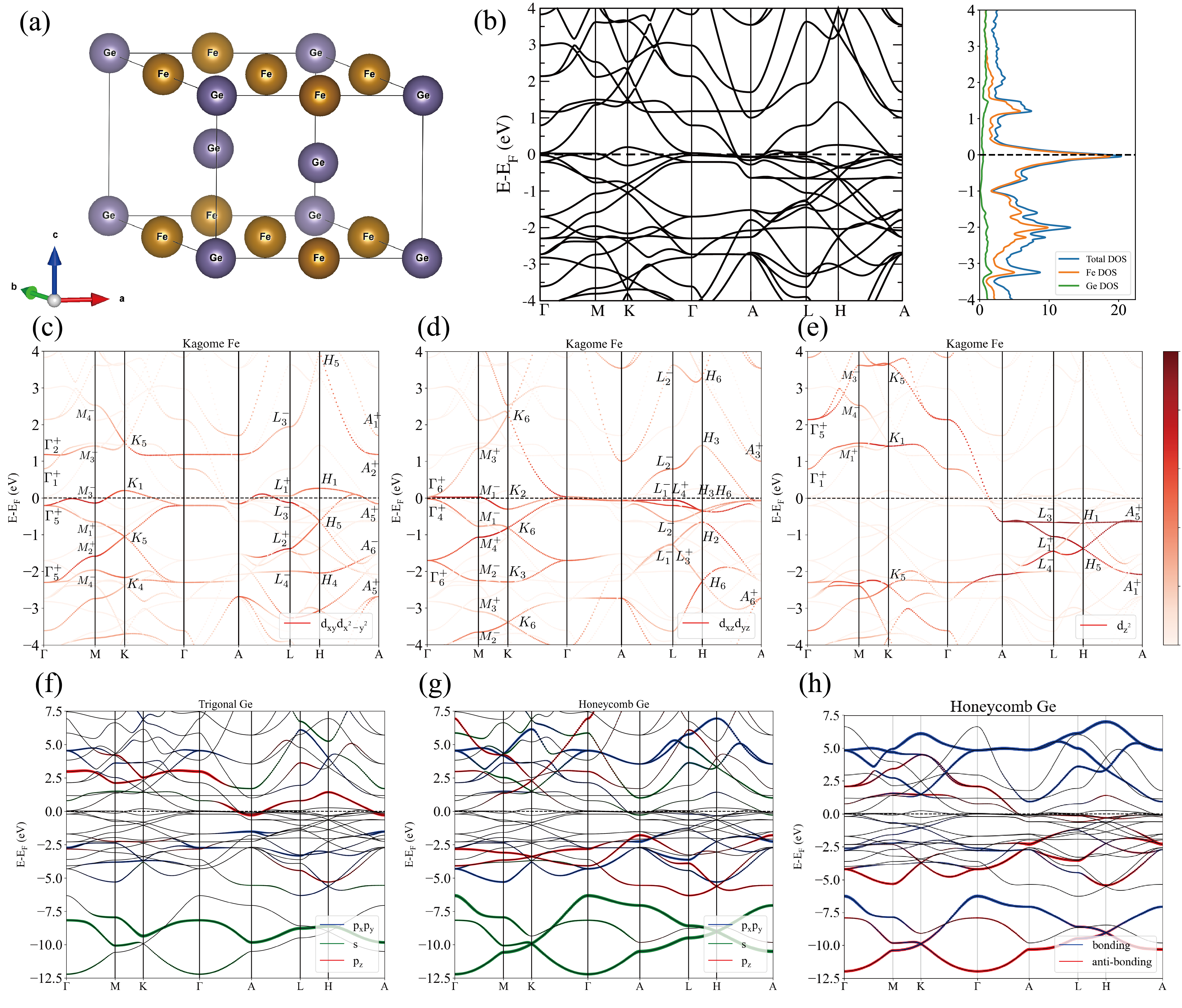
Figure S4: (a) Crystal structure and (b) band structure and density of states (DOS) without SOC of FeGe in the paramagnetic phase. (c)-(h) are orbital projections of the bands in the PM phase of FeGe, where (c) is the projection of $d_{xy},d_{x^{2}-y^{2}}$ of Fe, (d) $d_{xz},d_{yz}$ of Fe, (e) $d_{z^{2}}$ of Fe, (f) $s,p$ orbitals of honeycomb Ge, (g) $s,p$ orbitals of trigonal Ge, and (h) the bonding and anti-bonding states formed by $x,p_{x},p_{y}$ orbitals of honeycomb Ge (see Section II.1). IRREPs are marked in (c)-(e) for three groups of $d$ orbitals.

I.3 Band structures

I.3.1 Paramagnetic phase

We use the Vienna ab-initio Simulation Package (VASP)Kresse and Furthmüller (1996a); Kresse and Hafner (1993a, b, 1994); Kresse and Furthmüller (1996b) to perform the ab-initio computations for PM and AFM phases of FeGe.

The paramagnetic (PM) band structure without spin-orbit coupling (SOC) is shown in Fig. S4(b), where the bands near the Fermi level are mainly contributed by the $d$ orbitals of Fe according to the orbital projections shown in Fig. S4(c)-(g). We label the band IRREPs for three groups of $d$ orbitals in (c)-(e), where the IRREP labels follow the convention in Bilbao Crystallographic Server (BCS)Aroyo et al. (2006a, b).

From the orbital projections, it can be seen that there are two quasi-flat bands near $E_{f}$, one from $(d_{xy},d_{x^{2}-y^{2}})$ while the other one from $(d_{xz},d_{yz})$ of Fe. $d_{z^{2}}$ orbitals also contribute a extremely flat band on $k_{3}=\pi$ plane at about $-0.5$ $eV$. The bands of $(d_{xy},d_{x^{2}-y^{2}})$ in energy range $[-2,0.5]$ eV are roughly the same on the $k_{z}=0,\pi$ planes, with von Hove singularities (vHS) at $M$ and $L$, and Dirac points at $K$ and $H$. However, for $(d_{xy},d_{x^{2}-y^{2}})$ and $d_{z^{2}}$, their bands on the $k_{z}=0,\pi$ planes change significantly.

I.3.2 Antiferromagnetic phase

In Fig. S5(b), (c) the AFM band structure without and with SOC computed from DFT. SOC has negligible effects on the band structure near $E_{f}$. The computed magnetic moment on each Fe atom is about $1.53$ $\mu_{B}$ from DFT, which is close to the experiment value of around $1.7$ $\mu_{B}$ in literatureOhoyama et al. (1963); Häggström et al. (1975b); Forsyth et al. (1978). The bands in the AFM phase are two-fold degenerate with the $d$ orbital bands consisting of spin-up orbitals from one kagome layer and spin-down orbitals from the other kagome layer, related by the anti-unitary translation $\mathcal{T}\cdot\{E|001\}$.

In Fig. S5(d)-(f), we show the $d$ orbital projections of Fe in the AFM bands without SOC. We use blue and red colors to denote $d$ orbitals of opposite spins from three Fe atoms on one kagome layer. The three Fe atoms on the other kagome layer have identical orbital projections, with spin-up and down bands reversed. There are two vHSs that are close to the Fermi level, with the one at $M$ mainly coming from the $d_{xy}$ and $d_{x^{2}-y^{2}}$ orbitals while the one at $L$ mainly from $d_{z^{2}}$ but has some mixing with $d_{xz}$ and $d_{yz}$ orbitals of Fe at kagome sites. The vHS at $M$ is 19 meV higher than the Fermi level, while the one at $L$ is 69 meV lower.

I.3.3 DFT calculation details

The ab-initio calculations in this work are performed using the Vienna ab-initio Simulation Package (VASP)Kresse and Furthmüller (1996b); Kaltak (2015) with generalized gradient approximation of Perdew-Burke-Ernzerhof (PBE) exchange-correlation potentialPerdew et al. (1996). The $8\times 8\times 8$ $k$-mesh and an energy cutoff of 500 eV are used for both self-consistency and cRPA computations ((see Appendix III)). The MLWFs are obtained using WANNIER90Mostofi et al. (2008). The local coordinate system defined in Eq. S2.7 is used in constructing MLWFs.

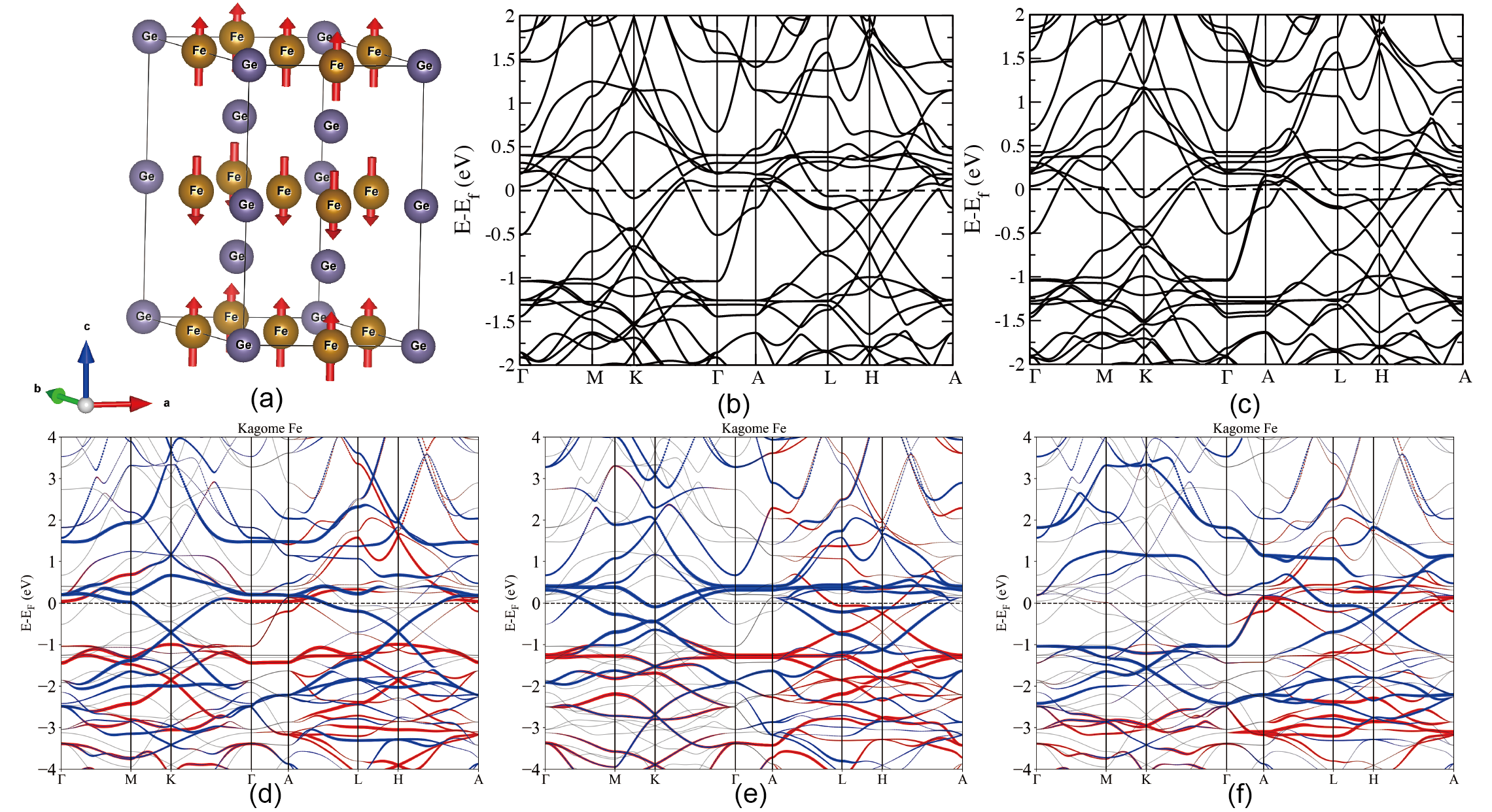
Figure S5: (a) Crystal structure, (b) band structure without SOC, and (c) band structure with SOC of FeGe in the AFM phase. (d)-(f) are orbital projections of the bands in the AFM phase of FeGe, where (c) is the projection of $d_{xy},d_{x^{2}-y^{2}}$ of Fe, (d) $d_{xz},d_{yz}$ of Fe, (e) $d_{z^{2}}$ of Fe, where blue and red colors denote $d$ orbitals of opposite spins of three Fe on one kagome plane.

Appendix II Tight-binding (TB) models of FeGe

In this section, we construct tight-binding (TB) Hamiltonians for FeGe. We first use maximally localized Wannier functions to construct faithful TBs as references. Then we construct three decoupled groups of minimal TB models that capture the main features of FeGe.

II.1 TB from Wannier functions

We first construct maximally localized Wannier functions (MLWFs) by Wannier90Marzari and Vanderbilt (1997); Souza et al. (2001); Marzari et al. (2012); Pizzi et al. (2020) to obtain onsite energies and hoppings parameters of orbitals and use the Wannier TB to calculate the filling and magnetic moments of each orbital in both PM and AFM phases.

To construct MLWFs, it is more convenient to use local coordinates on kagome sites $3f$ to decouple the five $d$ orbitals. As shown in Fig. S6, the global coordinate system on each kagome site is the Cartesian coordinate, i.e.,

$$3f_{i}:\ \bm{x}_{i}=(1,0,0),\bm{y}_{i}=(0,1,0),\bm{z}_{i}=(0,0,1),$$ (S2.6)

while the local coordinates at each kagome site $3f_{i}$ are defined as (same for kagome site $3g$):

$$3f_{1}: \bm{x}_{1}=(1,0,0),\bm{y}_{1}=(0,1,0),\bm{z}_{1}=(0,0,1)$$ (S2.7)

$$3f_{2}: \bm{x}_{2}=(\frac{1}{2},\frac{\sqrt{3}}{2},0),\bm{y}_{2}=(-\frac{\sqrt{3}}{2},\frac{1}{2},0),\bm{z}_{2}=(0,0,1)$$

$$3f_{3}: \bm{x}_{3}=(-\frac{1}{2},\frac{\sqrt{3}}{2},0),\bm{y}_{3}=(-\frac{\sqrt{3}}{2},-\frac{1}{2},0),\bm{z}_{3}=(0,0,1).$$

where the coordinates are written in Cartesian coordinates.

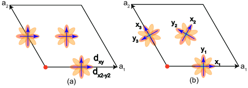
Figure S6: Definition of (a) global and (b) local coordinate systems on three kagome sites, with $d_{xy}$ and $d_{x^{2}-y^{2}}$ placed as representative orbitals. In (a), the coordinate system at three kagome sites is the same, i.e., along the global $x$ and $y$ direction, while in (b), the local coordinate system $(x_{1},y_{1})$ at $3f_{1}$ is the same as the global one, while $(x_{2},y_{2})$ at $3f_{2}$ and $(x_{3},y_{3})$ at $3f_{3}$ is rotated $\frac{\pi}{3}$ and $\frac{2\pi}{3}$ from the global one, respectively.

We first construct MLWFs in both the PM and AFM phases using a large orbital group, i.e., $s,p,d$ orbitals of Fe and $s,p$ orbitals of Ge, in order to give a faithful representation of the DFT band structure. In Table S4, we show the filling number of each orbital in the PM and AFM phases and the magnetic moments of $d$ orbitals in the AFM phase. The total fillings in the PM and AFM phases are close to 36, which is the number of valence electrons in FeGe used in DFT. We also plot the orbital projections and density of stats of five $d$ orbitals separately in both the PM and AFM phase in Fig. S7.

Note that the filling in Wannier TB is not exactly the number of electrons, because FeGe is a metallic system with numerous bands crossing $E_{f}$. The total filling (per PM unit cell) in the PM and AFM phases calculated from Wannier TB is 36.26 and 36.15, respectively (close to the number of valence electrons used in DFT, i.e., 36 from $s,p,d$ of 3 Fe and $s,p$ of 3 Ge). When constructing MLWFs, the dispersion and orbitals weights in the fitted Wannier bands could be slightly different from DFT, and the number of valence electrons is not fixed. In this case, the total filling of the orbitals considered may be slightly different. If we enforce the total filling to be the same as DFT in Wannier, $E_{f}$ would be about 25 $meV$ lower, which is insignificant as the Wannier filling does not deviate much from the DFT value.

	Orbitals	$s$	$p_{z}$	$p_{x}$	$p_{y}$	$d_{z^{2}}$	$d_{xz}$	$d_{yz}$	$d_{x^{2}-y^{2}}$	$d_{xy}$	Total
PM filling	Fe	0.35	0.22	0.25	0.26	1.54	1.72	1.56	1.42	1.57	8.88
	Tri-Ge	1.28	0.36	0.75	0.75	-	-	-	-	-	3.12
	Hon-Ge	1.26	0.74	0.60	0.60	-	-	-	-	-	3.25
AFM filling	Fe	0.24	0.25	0.25	0.25	1.66	1.63	1.48	1.49	1.62	8.87
	Tri-Ge	1.19	0.44	0.76	0.76	-	-	-	-	-	3.14
	Hon-Ge	1.13	0.83	0.65	0.65	-	-	-	-	-	3.20
AFM magmom	Fe	-	-	-	-	0.19	0.38	0.42	0.45	0.12	1.56
PM DOS@$E_{f}$	Fe	-	-	-	-	0.02	0.21	0.31	0.33	0.06	0.93
AFM DOS@$E_{f}$	Fe	-	-	-	-	0.08	0.20	0.21	0.23	0.05	0.77
PM filling $\in[-2,2]$	Fe	0.01	0.04	0.06	0.05	0.73	1.25	0.89	0.66	0.84	4.54

Table S4: The filling, magnetic moments (magmom), and density of states (DOS) at the Fermi level ($E_{f}$) of each orbital in the PM and AFM phase. All values are computed using the TB model from MLWFs constructed using $s,p,d$ orbitals of Fe and $s,p$ orbitals of Ge. The filling numbers are averaged over atoms on the same Wyckoff positions. In the PM phase, the fillings have timed 2 to account for two degenerate spins. The DOS at $E_{f}$ is normalized to 1 for the orbitals considered in the model. In the last row, we also list the fillings computed for bands $\in[-2,2]$ eV, which will be used as the reference for constructing minimal TB models in the next section. The total filling (per PM unit cell) in the PM and AFM phases is 36.26 and 36.15, respectively, which is close to the number of valence electrons used in DFT, i.e., 36 from $4s^{1}3d^{7}$ of 3 Fe ($3p^{6}$ are core states and not included in the Wannier TB, and the $p$ orbitals of Fe in the table are $4p$) and $4s^{2}4p^{2}$ of 3 Ge. Notice that the fillings of $4s$ and $4p$ orbitals of Fe are very small, which is a result of charge transfer between $3d$ of Fe and other orbitals of Ge.

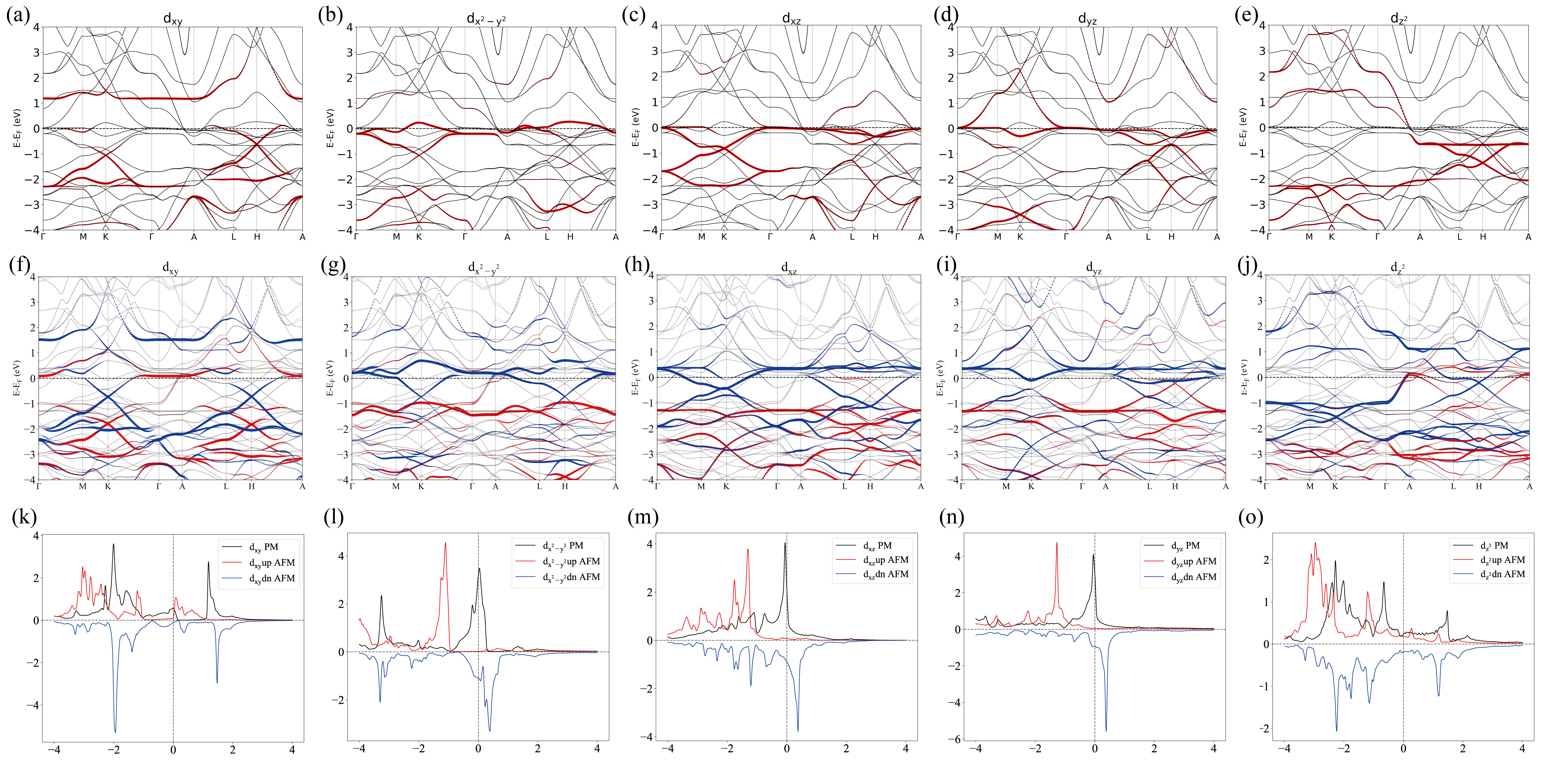
Figure S7: The band projections of five $d$ orbital of Fe in PM phase (a)-(e) and AFM phase (f)-(j), and density of states (DOS) in (h)-(l), obtained from MLWFs where local coordinates defined in Eq. S2.7 are used in order to separate $d$ orbitals. In (f)-(j), the blue and red colors denote two opposite spins, where only three Fe atoms on the same kagome layer are considered, as the other three Fe atoms have the reversed spin distributions enforced by the anti-unitary translation $\mathcal{T}\cdot\{E|0,0,1\}$.

We then construct another group of MLWFs using a smaller number of orbitals, i.e., $d$ orbitals of Fe and $s,p$ orbitals of Ge, which have 27 orbitals in total. Other orbitals, e.g., $s,p$ orbitals of Fe, have main distributions far from the Fermi level $E_{f}$, thus having little effect on the low-energy physics.

To construct this group of MLWFs, we first replace the $s,p_{x},p_{y}$ orbitals of honeycomb Ge by $s$ (bonding) and $p_{y}$ (anti-bonding) orbitals at kagome sites $3g$. This can be understood from the analog with graphene, where the carbon atoms at honeycomb sites $2d$ have their $p_{z}$ orbitals form Dirac cones near $E_{f}$ while $s,p_{x},p_{y}$ orbitals form $sp^{2}$ hybrid bonding and anti-bonding states that distribute mainly below and above $E_{f}$, respectively. From the elementary band representations (EBRs)Bradlyn et al. (2017); Cano et al. (2018); Elcoro et al. (2021), $A_{1}^{\prime}(s)@2d+E^{\prime}(p_{x},p_{y})@2d$ is (irrrep-)equivalent to $A_{g}(s)@3g+B_{2u}(p_{y})@3g$, which means the $sp^{2}$ hybrid orbitals on honeycomb sites $2d$ is equivalent to the $s$ and $p_{y}$ orbitals on kagome site $3g$. The real-space invariantXu et al. (2021b) for $s,p_{x},p_{y}@2d$ and $s,p_{y}@3g$ are both zero, which verifies that they can transform to each other. The $s@3g$ orbitals form the bonding states distributed mainly below $E_{f}$ while $p_{y}@3g$ orbitals form the anti-bonding states mainly above $E_{f}$, which can be verified from the IRREPs and orbital projections, as shown in Fig. S4(h). The reason for this basis transformation is that the $p_{x},p_{y}$ orbitals of honeycomb Ge form only one EBR but have distributions both below and above $E_{f}$ and cannot be decomposed into two EBRs. Thus we include the $s$ orbitals to form two separated $sp^{2}$ hybrid states, which will facilitate further analysis. We also remark that the inclusion of $s$ orbitals of Ge is helpful to increase the locality of $d$ orbitals and reduces long-range hoppings. A hopping truncation of $0.1$ results in a reasonably good band structure compared with DFT.

The onsite energy and nearest neighbor (NN) hoppings of this 27-band tight-binding model from MLWFs are listed in Table S5 for reference. It can be seen that the onsite energies of five $d$ orbitals of Fe have close values of about $-1$ eV, which may result from a quasi-cubic crystal field formed by 6 closed Ge atoms around a Fe atom. In Sec.III.3, we will use this quasi-cubic crystal field to simplify the Coulomb interaction matrix, and more details can be found there. The $p$ orbitals of trigonal and honeycomb Ge, however, have very different onsite energies, which results from their different chemical environments, i.e., trigonal Ge has Fe atoms on the same plane but honeycomb Ge has not.

Orbital	$d_{xy}$	$d_{x^{2}-y^{2}}$	$d_{xz}$	$d_{yz}$	$d_{z^{2}}$	Tri $s$	Tri $p_{x}$	Tri $p_{y}$	Tri $p_{z}$	Hon $p_{z}$	$sp^{2}$-$b$	$sp^{2}$-$ab$
onsite energy	-1.15	-1.00	-0.89	-0.84	-1.10	-8.08	-0.42	-0.42	0.60	-1.41	-4.64	0.93
$d_{xy}$	0.53	0.01	-	-	-0.16	-	0.00	0.73	-	-	-	-
$d_{x^{2}-y^{2}}$	-0.01	-0.47	-	-	-0.18	-0.66	-0.86	0.00	-	-0.54	0.23	-
$d_{xz}$	-	-	-0.20	-0.16	-	-	-	-	0.58	-	-	-
$d_{yz}$	-	-	0.16	0.29	-	-	-	-	-	0.77	-	-1.17
$d_{z^{2}}$	0.16	-0.18	-	-	-0.22	0.51	0.68	0.00	-	0.05	-1.07	-

Table S5: The onsite energy and NN hoppings of the 27-band TB model from Wannier functions. The second row lists the onsite energy of each orbital, and the other rows are the NN hoppings. ‘Tri $p_{i}$’ and ‘Hon $p_{i}$’ denote the $p_{i}$ orbitals at trigonal and honeycomb sites and $sp^{2}$-$b$ (-$ab$) denote the bonding (anti-bonding) states formed by $s,p_{x},p_{y}$ orbitals of honeycomb Ge. The onsite hopping from $d_{x^{2}-y^{2}}$ to $d_{z^{2}}$ is $-0.17$, which is not listed in the table. The label ‘-’ in the table means the NN hopping is forbidden by symmetries. The hopping parameter $t_{ij}$ is from the $d_{i}@3f_{1}$ orbital of each row to $d_{j}@3f_{2},s,p@1a,p_{z}@2c_{2},b,ab@3g_{1}$ labeled for each column. All numbers are in eV.

II.2 Separation of orbitals into three groups

The 27-band TB model obtained from MLWFs can serve as a good starting point for further studies. However, it still contains a large number of orbitals and hopping parameters. The longer-range hoppings beyond NN cannot be discarded directly, as the resultant band structure will deviate significantly from the original TB model. It is desirable to construct minimal TB models that contain fewer orbitals and have only NN or a few longer-range hoppings but could reproduce important features in the band structure, including the flat bands and van Hove singularities.

To fulfill this goal, we extract three groups of orbitals from the 27 orbitals of the Wannier TB, with the hoppings between orbitals from different groups being relatively weak. Therefore, we can construct the TB models for each group separately. The three groups of orbitals are

• $(d_{xy},d_{x^{2}-y^{2}})$ orbitals of Fe on the kagome sites and $(p_{x},p_{y})$ orbitals of trigonal Ge, i.e., 8 orbitals in total.

• $(d_{xz},d_{yz})$ orbitals of Fe on kagome sites, $p_{z}$ orbital of honeycomb Ge and $p_{z}$ orbital of trigonal Ge, i.e., 9 orbitals in total.

• $d_{z^{2}}$ orbitals of Fe and the $sp^{2}$ bonding states of honeycomb Ge, i.e., 6 orbitals in total.

Figure S8: Decomposition of three sets of orbitals. (a) $d_{x^{2}-y^{2}},d_{xy}$ of kagome Fe and $p_{x},p_{y}$ of trigonal Sn ($d_{xy}$ is omitted in the plot for simplicity). (b) $d_{xz},d_{yz}$ of kagome Fe and $p_{z}$ of trigonal and honeycomb Sn ($d_{yz}$ is omitted for simplicity). (c) $d_{z^{2}}$ of kagome Fe and the bonding state (equivalent to $s$ orbital on $z=\frac{1}{2}$ plane) of honeycomb Sn.

We now justify the reason for this separation. We first consider the separation of five $d$ orbitals of Fe. Under symmetries of SG 191, $d$ orbitals on kagome sites naturally split into three groups, i.e., $(d_{xy},d_{x^{2}-y^{2}})$, $(d_{xz},d_{yz})$, and $d_{z^{2}}$. The hoppings between $(d_{xz},d_{yz})$ and the other two groups of $d$ orbitals are forbidden on the $z=0$ plane, as $M_{z}$ is an onsite symmetry and these orbitals have opposite $M_{z}$ eigenvalues, while the inter-kagome layer hoppings are much smaller as the distance is long. Moreover, the hoppings between $(d_{xy},d_{x^{2}-y^{2}})$ and $d_{z^{2}}$ are also relatively small from the 27-band Wannier TB model in Table S5. This comes from the different shapes of the wavefunctions, i.e., the amplitudes of $(d_{xy},d_{x^{2}-y^{2}})$ wavefunctions mostly come from the $xy$ planes, while the amplitudes of $d_{z^{2}}$ wavefunctions mostly come from the $z$-axis. This results in a small overlap between the wavefunction of $d_{z^{2}}$ and $d_{xy},d_{x^{2}-y^{2}}$ orbitals. Notice that since $d_{x^{2}-y^{2}}$ and $d_{z^{2}}$ belong to the same trivial IRREP of $D_{2h}$, they have a small onsite hopping of -0.17 eV. A proper linear combination of $d_{x^{2}-y^{2}}$ and $d_{z^{2}}$ could remove the onsite hopping (note the simple equal-weight combination fails as they do not have the same onsite energy), but would make the basis more complicated. Thus we omit it for simplicity. Therefore, we conclude that three groups of $d$ orbitals can be analyzed separately. As for the $s$ and $p$ orbitals of Fe, they are far from the Fermi level $E_{f}$ and are omitted.

We then consider the orbitals of Ge, which do not have many contributions near $E_{f}$. They are used as auxiliary orbitals in order to describe the dispersion of $d$ orbitals of Fe near $E_{f}$ more faithfully. For trigonal Ge, we consider $(p_{x},p_{y})$ and $p_{z}$ orbitals, and omit its $s$ orbital which is far from $E_{f}$, as shown in Table. S5 (although tri-$s$ has a large hopping (-0.66$eV$) to $d_{x^{2}-y^{2}}$, the large onsite difference makes the effect of tri-$s$ on $d_{x^{2}-y^{2}}$ negligible). For honeycomb Ge’s, we consider the $p_{z}$ and the bonding states formed by $s,p_{x},p_{y}$ orbitals (see Section II.1 for more details about the bonding states). These orbitals have non-negligible hybridization with $d$ orbitals of Fe. Denote these orbitals as $p_{x}^{t},p_{y}^{t},p_{z}^{t},p_{z}^{h},b$, where the superscript $t$ and $h$ denote trigonal and honeycomb, and $b$ denotes the bonding states of honeycomb Ge.

Finally, we combine the three groups of $d$ orbitals with specific orbitals of Ge.

1. $(d_{xy},d_{x^{2}-y^{2}})$ orbitals of Fe and $(p_{x}^{t},p_{y}^{t})$ orbitals of trigonal Ge. These orbitals form a bipartite crystalline lattice (BCL) with 8 bands. The reason to combine $(d_{xy},d_{x^{2}-y^{2}})$ with $(p_{x}^{t},p_{y}^{t})$ orbitals is that they all lie on the $z=0$ plane and have large overlaps which result in $\sigma$-like bonds. This can be verified from the large hopping parameters from the Wannier TB in Table S5, as well as the overlap of orbital projections in DFT in Fig. S4.

2. $(d_{xz},d_{yz})$ orbitals of Fe and $p_{z}$ orbitals of honeycomb and trigonal Ge. These orbitals are all along the $z$-direction and have large overlaps that form $\pi$-like bonds, verified from Wannier hoppings and orbital projections. The $sp^{2}$ anti-bonding states of honeycomb Ge, although have large hoppings with $d_{yz}$, lie high above the Fermi level. We do not consider them directly but add $z$-directional hoppings to $d_{yz}$, which can be seen as the indirect hopping given by the anti-bonding states.

3. $d_{z^{2}}$ orbitals of Fe and the $sp^{2}$ bonding states of honeycomb Ge. For this group of orbitals, the bands close to $E_{f}$ come mainly from $d_{z^{2}}$. However, the $d_{z^{2}}$ dispersion has a large splitting about $5$ eV on the $k_{z}=0$ plane but has an almost standard $s$-orbital kagome dispersion with a flat band on the $k_{3}=\pi$ plane (Fig. S4). This band structure cannot be faithfully reproduced using $d_{z^{2}}$ orbitals only (with NN or NNN hoppings the $d_{z^{2}}$ bands are connected and cannot give the split bands on $k_{z}=0$ plane) but needs the assistance of other orbitals, i.e., the bonding states, which have the largest hopping with $d_{z^{2}}$. However, if we are only interested in the low energy physics near $E_{f}$, we can perturb out the bonding states and use the $d_{z^{2}}$ alone to build the TB model. In this case, the Coulomb interaction of $d_{z^{2}}$ also needs to be renormalized to a smaller value as the weight of $d_{z^{2}}$ near $E_{f}$ is increased when the bonding states are perturbed out. We also remark that the couplings between $d_{z^{2}}$ and the first group of orbitals, although existing in the Wannier TB, are not considered as an approximation due to their relatively small hopping values and thus minor effects for bands near $E_{f}$.

In the following sections, we first use the three aforementioned groups of orbitals to construct three minimal TB models that can reproduce the band structures in the PM phase and use the $S$-matrix formalismCălugăru et al. (2022) of generalized bipartite lattices to explain the quasi-flat bands near the Fermi level. We then combine these models together with extra coupling terms between $d_{x^{2}-y^{2}}$ and honeycomb $p_{z}$ and use second-order perturbations to perturb out the coupling terms and obtain three decoupled models.

In Section II.3.1, we build $H_{1}(\mathbf{k})$ model for $(d_{xy},d_{x^{2}-y^{2}})$ of Fe and $(p_{x}^{t},p_{y}^{t})$ of trigonal Ge, which has only inplane hoppings and is $k_{z}$-independent. In Section II.3.2, we build $H_{2}(\mathbf{k})$ for $(d_{xz},d_{yz})$ of Fe and $p_{z}$ of both trigonal and honeycomb Ge. In Section II.3.3, we first build $H_{3}(\mathbf{k})$ for $d_{z^{2}}$ and $sp^{2}$ bonding states of honeycomb Ge. We then perturb out the bonding states and construct an effective $H_{3}(\mathbf{k})$ that only contains $d_{z^{2}}$. In Section II.3.4, we build the combined model by first coupling honeycomb $p_{z}^{h}$ with $d_{x^{2}-y^{2}}$ to introduce the $k_{z}$-dependence for $d_{x^{2}-y^{2}}$ and then perturb out this extra coupling term such that three $H_{i}(\mathbf{k})$ are still decoupled. We then further perturb out the trigonal $p_{z}^{t}$ in $H_{2}(\mathbf{k})$ which has negligible distribution near $E_{f}$. The final minimal TB model is the direct sum of three $H_{i=1,2,3}(\mathbf{k})$ with perturbation terms.

II.3 Minimal TB models for three groups of orbitals

We first give some preliminaries on the TB Hamiltonians. We adopt the Fourier transform convention of Bloch function

$$|\psi_{j}(\bm{k})\rangle=\frac{1}{\sqrt{N}}\sum_{\bm{R}}e^{i\bm{k}\cdot(\bm{R}+\bm{\tau}_{j})}|\phi_{\bm{R}j}\rangle.$$ (S2.8)

where $|\phi_{\bm{R}j}\rangle$ denotes the Wannier function basis, and $\bm{\tau}_{j}$ is the Wyckoff position of these Wannier functions in the unit cell. In this convention, the hopping matrix is

$$H_{ij}(\bm{k})=\langle\psi_{i}(k)|\hat{H}_{t}|\psi_{j}(k)\rangle=\sum_{\bm{R}}e^{i\bm{k}\cdot(\bm{R}+\bm{\tau}_{j}-\bm{\tau}_{i})}H_{ij}(\bm{R})$$ (S2.9)

where $H_{ij}(\bm{R})=\langle\phi_{\bm{0},i}|\hat{H}|\phi_{\bm{R}j}\rangle$ is the hopping between Wannier functions. Note that the Hamiltonian in this convention is not periodic in the Brillouin zone (BZ), i.e., $H(\bm{k}+\bm{G})=V^{\dagger}(\bm{G})H(\bm{k})V(\bm{G})$, where $V(\bm{G})_{ij}=e^{i\bm{G}\cdot\bm{\tau}_{i}}\delta_{ij}$ is the embedding matrix.

The TB Hamiltonian satisfies the symmetry constraints

$$D^{-1}(g)H(\bm{k})D(g) =H(g^{-1}\bm{k}),\quad g\text{ unitary},$$ (S2.10)

$$D^{-1}(g)H^{*}(\bm{k})D(g) =H(g^{-1}\bm{k}),\quad g\text{ anti-unitary},$$

where $g\in G$ are symmetry operations of (magnetic) space group $G$, and $D(g)$ the representation matrix of $g$ under the TB basis $\psi_{i}(\bm{r})$ defined by $g\psi_{i}(\bm{r})=\psi_{i}(g^{-1}\bm{r})=D_{ij}(g)\psi_{j}(\bm{r})$, and $g\bm{k}$ denotes the action of $g$ on $\bm{k}$. We use the MagneticTBZhang et al. (2022b) package to generate the TB Hamiltonians, where Eq. S2.10 is used to solve the independent hopping parameters in the Hamiltonian that satisfy the symmetry.

For a high-symmetry point (HSP) $\bm{k}_{0}$ with little group $G_{\bm{k}_{0}}$, assume $g^{-1}\bm{k}=\bm{k}+\bm{G}_{g}$, then

$$D^{-1}(g)H(\bm{k})D(g)=H(\bm{k}+\bm{G}_{g}) =V^{\dagger}(\bm{G}_{g})H(\bm{k})V(\bm{G}_{g})$$ (S2.11)

$$\Rightarrow[H(\bm{k}),D(g)V^{\dagger}(\bm{G}_{g})] =0$$

Thus $D^{\prime}(g)=D(g)V^{\dagger}(\bm{G}_{g})$ has common eigenstates with $H(\bm{k})$. This relation can be used to compute the IRREPs of bands of TB models.

When the bases of a TB Hamiltonian are divided into two groups, e.g., $p$ and $d$, which have representation matrices $D_{p}(g)$ and $D_{d}(g)$ of operation $g$, the S-matrix $S_{p,d}(\bm{k})$ which describes the coupling between $p$ and $d$ orbitals satisfies

$$D_{p}^{-1}(g)S_{p,d}(\bm{k})D_{d}(g)=S_{p,d}(g^{-1}\bm{k}).$$ (S2.12)

This equation can be used to check whether the elements of the S-matrix are forbidden by symmetries.

II.3.1 $H_{1}(k)$: $d_{xy},d_{x^{2}-y^{2}}$ of Fe and $p_{x},p_{y}$ of trigonal Ge

The first group of orbitals consists of $d_{xy},d_{x^{2}-y^{2}}$ orbitals of Fe and $p_{x},p_{y}$ orbitals of Ge at trigonal sites, which form a bipartite crystalline lattice (BCL) of 8 bands. The band representations (BRs) are the superposition of three elementary BRs (EBRs), i.e., $E_{1u}@1a,A_{g}@3f,B_{1g}@3f$, where $E_{1u}$, $A_{g}$, and $B_{1g}$ are the IRREPs formed by $(p_{x},p_{y})$, $d_{xy}$, and $d_{x^{2}-y^{2}}$ orbitals, respectively, as shown in Table S3. We use $3f_{1}$, $3f_{2}$, and $3f_{3}$ to denote the three kagome lattice sites listed in Table S2.

We first use a global coordinate system on kagome sites to define orbitals, which is more straightforward and is the default choice in many softwaresZhang et al. (2022b), and then transform it into the local coordinate system defined in Eq. S2.7. We choose the TB basis under the global coordinate system as

$$\psi_{\text{glob}}=(p_{x}@1a,p_{y}@1a,d_{xy}@3f_{1},d_{x^{2}-y^{2}}@3f_{1},d_{xy}@3f_{2},d_{x^{2}-y^{2}}@3f_{2},d_{xy}@3f_{3},d_{x^{2}-y^{2}}@3f_{3}),$$ (S2.13)

The generators of SG 191 have the following $O(3)$ matrices under the conventional basis defined in Eq. S1.5:

$$C_{6z}=\left(\begin{matrix}1&-1&0\\ 1&0&0\\ 0&0&1\\ \end{matrix}\right),\quad C_{2,110}=\left(\begin{matrix}0&1&0\\ 1&0&0\\ 0&0&-1\\ \end{matrix}\right),\quad P=\left(\begin{matrix}-1&0&0\\ 0&-1&0\\ 0&0&-1\\ \end{matrix}\right),\quad$$ (S2.14)

and representation matrices under the TB basis defined in Eq. S2.13 using the global coordinate system

$$D_{\text{glob}}(C_{6z})=\left(\begin{matrix}\frac{1}{2}&-\frac{\sqrt{3}}{2}&0&0&0&0&0&0\\ \frac{\sqrt{3}}{2}&\frac{1}{2}&0&0&0&0&0&0\\ 0&0&0&0&0&0&-\frac{1}{2}&\frac{\sqrt{3}}{2}\\ 0&0&0&0&0&0&-\frac{\sqrt{3}}{2}&-\frac{1}{2}\\ 0&0&-\frac{1}{2}&\frac{\sqrt{3}}{2}&0&0&0&0\\ 0&0&-\frac{\sqrt{3}}{2}&-\frac{1}{2}&0&0&0&0\\ 0&0&0&0&-\frac{1}{2}&\frac{\sqrt{3}}{2}&0&0\\ 0&0&0&0&-\frac{\sqrt{3}}{2}&-\frac{1}{2}&0&0\\ \end{matrix}\right),\quad$$ (S2.15)

$$D_{\text{glob}}(C_{2,110})=\left(\begin{matrix}-\frac{1}{2}&\frac{\sqrt{3}}{2}&0&0&0&0&0&0\\ \frac{\sqrt{3}}{2}&\frac{1}{2}&0&0&0&0&0&0\\ 0&0&0&0&0&0&\frac{1}{2}&-\frac{\sqrt{3}}{2}\\ 0&0&0&0&0&0&-\frac{\sqrt{3}}{2}&-\frac{1}{2}\\ 0&0&0&0&\frac{1}{2}&-\frac{\sqrt{3}}{2}&0&0\\ 0&0&0&0&-\frac{\sqrt{3}}{2}&-\frac{1}{2}&0&0\\ 0&0&\frac{1}{2}&-\frac{\sqrt{3}}{2}&0&0&0&0\\ 0&0&-\frac{\sqrt{3}}{2}&-\frac{1}{2}&0&0&0&0\\ \end{matrix}\right),\quad$$ (S2.16)

$$D(P)=\text{Diag}(-1,-1,1,1,1,1,1,1)$$ (S2.17)

The TRS in the NSOC setting is $D(T)=\bm{1}_{8}$, where the complex conjugation is absorbed in the definition of symmetry constraints in Eq. S2.10.

Under the global coordinate system, the two $d$ orbitals are entangled under SG 191 operations, as can be seen from the representation matrices. In order to separate them, we transform the basis into local coordinates as shown in Fig. S6(b), with the coordinates at each kagome site defined in Eq. S2.7. Choose the TB basis under the local coordinate system as

$$\psi_{\text{loc}}=(p_{x}@1a,p_{y}@1a,d_{xy}@3f_{1},d_{xy}@3f_{2},d_{xy}@3f_{3},d_{x^{2}-y^{2}}@3f_{1},d_{x^{2}-y^{2}}@3f_{2},d_{x^{2}-y^{2}}@3f_{3}),$$ (S2.18)

Here the $d_{xy},d_{x^{2}-y^{2}}$ are under local coordinates and are rotated from the original $d$ orbitals, related to $\psi_{\text{glob}}$ by $\psi_{\text{loc}}^{T}=C_{2}C_{1}\psi_{\text{glob}}^{T}$, where $C_{1}$ is the global to local coordinate transformation and $C_{2}$ is a rearrangement of basis, defined by

$$C_{1}=\left(\begin{matrix}1&0&&&&&&\\ 0&1&&&&&&\\ &&1&0&&&&\\ &&0&1&&&&\\ &&&&-\frac{1}{2}&-\frac{\sqrt{3}}{2}&&\\ &&&&\frac{\sqrt{3}}{2}&-\frac{1}{2}&&\\ &&&&&&-\frac{1}{2}&\frac{\sqrt{3}}{2}\\ &&&&&&-\frac{\sqrt{3}}{2}&-\frac{1}{2}\\ \end{matrix}\right),\quad C_{2}=\left(\begin{matrix}1&0&&&&&&\\ 0&1&&&&&&\\ &&1&0&0&0&0&0\\ &&0&0&1&0&0&0\\ &&0&0&0&0&1&0\\ &&0&1&0&0&0&0\\ &&0&0&0&1&0&0\\ &&0&0&0&0&0&1\\ \end{matrix}\right).$$ (S2.19)

The representation matrices $D_{\text{loc}}(g)$ under $\psi_{\text{loc}}$ is related to $D_{\text{glob}}(g)$ by

$$D_{\text{loc}}(g)=C_{2}C_{1}D_{\text{glob}}(g)C_{1}^{-1}C_{2}^{-1},$$ (S2.20)

which results in

$$D_{\text{loc}}(C_{6z})=\left(\begin{matrix}\frac{1}{2}&-\frac{\sqrt{3}}{2}&&&&&&\\ \frac{\sqrt{3}}{2}&\frac{1}{2}&&&&&&\\ &&0&0&1&&&\\ &&1&0&0&&&\\ &&0&1&0&&&\\ &&&&&0&0&1\\ &&&&&1&0&0\\ &&&&&0&1&0\\ \end{matrix}\right),\quad D_{\text{loc}}(C_{2,110})=\left(\begin{matrix}-\frac{1}{2}&\frac{\sqrt{3}}{2}&&&&&&\\ \frac{\sqrt{3}}{2}&\frac{1}{2}&&&&&&\\ &&0&0&-1&&&\\ &&0&-1&0&&&\\ &&-1&0&0&&&\\ &&&&&0&0&1\\ &&&&&0&1&0\\ &&&&&1&0&0\end{matrix}\right),$$ (S2.21)

and $D_{\text{loc}}(P)=D_{\text{glob}}(P),D_{\text{loc}}(T)=D_{\text{glob}}(T)$.

In the following, we first give the general form of the TB Hamiltonian constrained by symmetries operations defined in Eq. S2.21, and then fit the hopping parameters to the DFT results, which matches correctly with the IRREPs and the main feature of the orbital projections in DFT. The hopping parameters obtained are effective hoppings that can be seen as the superposition of hoppings from several near neighbors. Remark that the near-neighbor hoppings obtained in the Wannier TB (Table S5) cannot be used directly, as there exist longer-range hoppings and also hybridizations with other orbitals in the Wannier TB. Moreover, as the onsite energies of Fe $d$ and Ge $p$ in the Wannier TB are close, a direct second-order perturbation does not work well. Thus we only use hoppings in the Wannier TB as a reference and refit the hoppings in the minimal TB model.

Considering a few near neighbor hoppings of the kagome lattice and hoppings between the kagome lattice and trigonal lattice, we construct the following TB model in the local coordinates basis $\psi_{\text{loc}}$, where we use $p_{xy}^{t}$ to denote $p_{x},p_{y}$ of trigonal Ge and $d_{1},d_{2}$ to denote $d_{xy},d_{x^{2}-y^{2}}$ in the local coordinates:

$$H_{1}(\bm{k})=\left(\begin{matrix}H_{p_{xy}^{t}}(\bm{k})&S_{p_{xy}^{t},d_{1}}(\bm{k})&S_{p_{xy}^{t},d_{2}}(\bm{k})\\ &H_{d_{1}}(\bm{k})&S_{d_{1},d_{2}}(\bm{k})\\ h.c.&&H_{d_{2}}(\bm{k})\\ \end{matrix}\right),$$ (S2.22)

$$H_{p_{xy}^{t}}(\bm{k}) =\mu_{p_{xy}^{t}}\mathbf{1}_{2},$$ (S2.23)

$$H_{d_{1}}(\bm{k}) =\mu_{d_{1}}\mathbf{1}_{3}+2t_{d_{1}}^{NN}H_{\text{Kagome}}^{\text{inplane,NN}}(\bm{k})+2t_{d_{1}}^{NNN}H_{\text{Kagome}}^{\text{inplane,NNN}}(\bm{k})$$

$$+2t_{d}^{4N1}\text{Diag}\left[\cos(k_{1}),\cos(k_{1}+k_{2}),\cos(k_{2})\right]$$

$$+2t_{d}^{4N2}\text{Diag}\left[\cos(k_{2})+\cos(k_{1}+k_{2}),\cos(k_{1})+\cos(k_{2}),\cos(k_{1})+\cos(k_{1}+k_{2})\right]$$

$$H_{d_{2}}(\bm{k}) =\mu_{d_{2}}\mathbf{1}_{3}+2t_{d_{2}}^{NN}H_{\text{Kagome}}^{\text{inplane,NN}}(\bm{k})+2t_{d_{2}}^{NNN}H_{\text{Kagome}}^{\text{inplane,NNN}}(\bm{k})$$

$$+2t_{d}^{4N1}\text{Diag}\left[\cos(k_{1}),\cos(k_{1}+k_{2}),\cos(k_{2})\right]$$

$$+2t_{d}^{4N3}\text{Diag}\left[\cos(k_{2})+\cos(k_{1}+k_{2}),\cos(k_{1})+\cos(k_{2}),\cos(k_{1})+\cos(k_{1}+k_{2})\right]$$

$$S_{d_{1},d_{2}}(\bm{k}) =2t_{d_{1},d_{2}}^{NN}\left(\begin{matrix}0&\cos(\frac{k_{2}}{2})&-\cos(\frac{k_{1}+k_{2}}{2})\\ -\cos(\frac{k_{2}}{2})&0&\cos(\frac{k_{1}}{2})\\ \cos(\frac{k_{1}+k_{2}}{2})&-\cos(\frac{k_{1}}{2})&0\\ \end{matrix}\right)$$

$$+2t_{d_{1},d_{2}}^{NNN}\left(\begin{matrix}0&\cos(k_{1}+\frac{k_{2}}{2})&-\cos(\frac{k_{1}-k_{2}}{2})\\ -\cos(k_{1}+\frac{k_{2}}{2})&0&\cos(\frac{k_{1}}{2}+k_{2})\\ \cos(\frac{k_{1}-k_{2}}{2})&-\cos(\frac{k_{1}}{2}+k_{2})&0\\ \end{matrix}\right)$$

$$+\sqrt{3}(t_{d}^{4N2}-t_{d}^{4N3})\text{Diag}\left[\cos(k_{2})-\cos(k_{1}+k_{2}),\cos(k_{1})-\cos(k_{2}),-\cos(k_{1})+\cos(k_{1}+k_{2})\right]$$

$$S_{p_{xy}^{t},d_{1}}(\bm{k}) =t_{p_{xy}^{t},d_{1}}^{NN}\left(\begin{matrix}0&i\sqrt{3}\sin(\frac{k_{1}+k_{2}}{2})&i\sqrt{3}\sin(\frac{k_{2}}{2})\\ -2i\sin(\frac{k_{1}}{2})&-i\sin(\frac{k_{1}+k_{2}}{2})&i\sin(\frac{k_{2}}{2})\\ \end{matrix}\right)$$

$$+t_{p_{xy}^{t},d_{1}}^{NNN}\left(\begin{matrix}-2i\sin(\frac{k_{1}}{2}+k_{2})&i\sin(\frac{k_{1}-k_{2}}{2})&-i\sin(k_{1}+\frac{k_{2}}{2})\\ 0&i\sqrt{3}\sin(\frac{k_{1}-k_{2}}{2})&i\sqrt{3}\sin(k_{1}+\frac{k_{2}}{2})\\ \end{matrix}\right)$$

$$S_{p_{xy}^{t},d_{2}}(\bm{k}) =t_{p_{xy}^{t},d_{2}}^{NN}\left(\begin{matrix}-2i\sin(\frac{k_{1}}{2})&-i\sin(\frac{k_{1}+k_{2}}{2})&i\sin(\frac{k_{2}}{2})\\ 0&-i\sqrt{3}\sin(\frac{k_{1}+k_{2}}{2})&-i\sqrt{3}\sin(\frac{k_{2}}{2}))\\ \end{matrix}\right)$$

$$H_{\text{Kagome}}^{\text{inplane,NN}}(\bm{k}) =\left(\begin{matrix}0&\cos(\frac{k_{2}}{2})&\cos(\frac{k_{1}+k_{2}}{2})\\ &0&\cos(\frac{k_{1}}{2})\\ c.c.&&0\\ \end{matrix}\right),\quad H_{\text{Kagome}}^{\text{inplane,NNN}}(\bm{k})=\left(\begin{matrix}0&\cos(k_{1}+\frac{k_{2}}{2})&\cos(\frac{k_{1}-k_{2}}{2})\\ &0&\cos(\frac{k_{1}}{2}+k_{2})\\ c.c.&&0\\ \end{matrix}\right)$$

where $c.c.$ denotes complex conjugation. In the model,

• $\mu_{p_{xy}^{t}}$ is the onsite energy of $p_{x,y}$ orbitals of Ge on trigonal lattice.

• $\mu_{d_{i}}(i=1,2)$ is the onsite energies of $d_{xy},d_{x^{2}-y^{2}}$ orbitals of Fe on kagome lattice.

• $t_{p_{xy}^{t},d_{i}}^{NN}$ are nearest-neighbor (NN) inter-sublattice hoppings from $p_{x},p_{y}$ to $d$ orbitals.

• $t_{d_{i}}^{NN},t_{d_{i}}^{NNN}$ are intra-kagome lattice NN and next nearest-neighbor (NNN) hoppings of $d_{xy},d_{x^{2}-y^{2}}$ orbitals, respectively.

• $t_{d_{1},d_{2}}^{NN},t_{d_{1},d_{2}}^{NNN}$ are the NN and NNN hoppings from $d_{xy}$ to $d_{x^{2}-y^{2}}$ orbitals on kagome lattice.

• $t_{d}^{4Ni}$ ($i=1,2,3$) are hoppings that across a unit cell for $d_{1}$ and $d_{2}$.

We do not include $z$-directional hoppings so that the band structures on $k_{3}=0,\pi$ planes are identical. A few long-range hoppings are also considered here to give a more faithful fit to the DFT bands. The $k_{3}$-dependence is introduced later in Sec.II.3.4 by considering coupling with $p_{z}$ orbitals of honeycomb Ge.

We discuss several ideal cases of the Hamiltonian S2.23 that host perfectly flat bands. Case #1 and #2 are unrealistic cases for FeGe but can help gain insight into the flat band limits and serve as applications of the $S$-matrix formalismCălugăru et al. (2022).

Case #1. When only considering inter-sublattice hoppings, the Hamiltonian is chiral symmetric, with the form

$$H_{1}(\bm{k})=\left(\begin{matrix}\bm{0}&S_{p_{xy}^{t},d_{1}}(\bm{k})&S_{p_{xy}^{t},d_{2}}(\bm{k})\\ S_{p_{xy}^{t},d_{1}}(\bm{k})^{\dagger}&\bm{0}&\bm{0}\\ S_{p_{xy}^{t},d_{2}}(\bm{k})^{\dagger}&\bm{0}&\bm{0}\\ \end{matrix}\right),$$ (S2.24)

The number of orbitals in trigonal and kagome lattices is $N_{p}=2$ and $N_{d}=6$, respectively. There are 4 perfectly flat bands at the Fermi level as shown in Fig. S9(a), which is the difference of orbital numbers in two sublatticesCălugăru et al. (2022); Regnault et al. (2022), i.e., $N_{d}-N_{p}=4$ (see Appendix VIII).

Case #2. When there is no hopping between three sets of orbitals and the kagome lattice has only NN hoppings, each kagome orbital has one perfectly flat band. In this case, the Hamiltonian is block-diagonal:

$$H_{1}(\bm{k})=\left(\begin{matrix}H_{p_{xy}^{t}}(\bm{k})&\bm{0}&\bm{0}\\ \bm{0}&H_{d_{1}}(\bm{k})&\bm{0}\\ \bm{0}&\bm{0}&H_{d_{2}}(\bm{k})\\ \end{matrix}\right),$$ (S2.25)

Case #3. When $S_{p_{xy}^{t},d_{1}}=0,H_{d_{2}}=\mu_{d_{2}}\mathbf{1}_{3},S_{d_{1},d_{2}}=0$, and $H_{d_{1}}$ has only NN hoppings, i.e.,

$$H_{1}(\bm{k})=\left(\begin{matrix}H_{p_{xy}^{t}}(\bm{k})&\bm{0}&S_{p_{xy}^{t},d_{2}}(\bm{k})\\ \bm{0}&H_{d_{1}}(\bm{k})&\bm{0}\\ S_{p_{xy}^{t},d_{2}}(\bm{k})^{\dagger}&\bm{0}&\mu_{d_{2}}\mathbf{1}_{3}\\ \end{matrix}\right),$$ (S2.26)

there will be 2 perfectly flat bands, one from $H_{d_{1}}(\bm{k})$ (decoupled) and the other one from $d_{x^{2}-y^{2}}$ (because $n_{d_{2}}-N_{p}=3-2=1$, where $n_{d_{2}}$ is the number of flat bands in $H_{d_{2}}$), as shown in Fig. S9(b).

Case #4. When $H_{d_{2}}=\mu_{d_{2}}\mathbf{1}_{3},S_{d_{1},d_{2}}=0$, i.e.,

$$H_{1}(\bm{k})=\left(\begin{matrix}H_{p_{xy}^{t}}(\bm{k})&S_{p_{xy}^{t},d_{1}}(\bm{k})&S_{p_{xy}^{t},d_{2}}(\bm{k})\\ S_{p_{xy}^{t},d_{1}}(\bm{k})^{\dagger}&H_{d_{1}}(\bm{k})&\bm{0}\\ S_{p_{xy}^{t},d_{2}}(\bm{k})^{\dagger}&\bm{0}&\mu_{d_{2}}\mathbf{1}_{3}\\ \end{matrix}\right),$$ (S2.27)

there will be one perfectly flat band from $d_{x^{2}-y^{2}}$, as shown in Fig. S9(c). This is because $H_{d_{2}}$ contributes 3 flat bands with the same energy $\mu_{d_{2}}$, which gives $3-2=1$ perfectly flat bands in $H_{1}(\bm{k})$. This agrees with the orbital projections in DFT in Fig. S7, where the quasi-flat band near the Fermi level mainly comes from $d_{x^{2}-y^{2}}$ orbital. In the following, we will verify why the effective hoppings values in DFT are close to this limit.

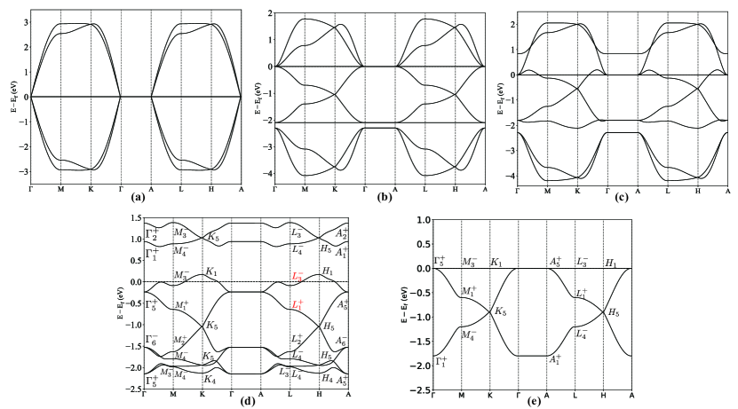
Figure S9: TB band structures of $d_{xy},d_{x^{2}-y^{2}}$ orbitals of Fe and $p_{x},p_{y}$ orbitals of trigonal Ge. (a) Case #1, chiral symmetric limit with 4 perfectly flat bands. (b) Case #3, two flat bands. (c) Case #4, one flat band. (d) General case to fit DFT band structure, with one quasi-flat band near Fermi level. (e) The band structure of $s$ orbital on kagome sites together with IRREPs. We label the IRREPs for bands in (d) and (e). In (d), the red IRREPs are mismatched with DFT bands (shown in Fig. S4), which is either far from $E_{f}$ (at $\Gamma$) or will be fixed later (at $L$) in Sec.II.3.4. The parameters in (d) are given in Table S9. The parameters in (c) are obtained from (d) by setting $H_{d_{2}}=\mu_{d_{2}}\bm{1}_{3},S_{d_{1},d_{2}}=\bm{0}$, $\mu_{p_{xy}^{t}}=-1.8,\mu_{d_{1}}=-1.25,\mu_{d_{2}}=0,t_{d_{1}}^{NN}=0.49,t_{d_{1}}^{NNN}=0.03,t_{p_{xy}^{t},d_{1}}^{NN}=0.82,t_{p_{xy}^{t},d_{1}}^{NN}=1.10$. The parameters in (b) are obtained from (c) by further setting $t_{d_{1}}^{NNN}=0,\mu_{p_{xy}^{t}}=-2.3$. The parameters in (a) are $t_{p_{xy}^{t},d_{1}}^{NN}=0.82,t_{p_{xy}^{t},d_{2}}^{NN}=1.23$ and all others zero.

Case #4 is closest to the DFT band structure among the four cases and serves as an explanation for the origin of the quasi-flat band in DFT. The perfect flat band becomes weakly dispersive when hoppings in $H_{d_{2}}(\bm{k})$ and $S_{d_{1},d_{2}}(\bm{k})$ are turned on. We fit the TB parameters to the DFT band structure based on dispersion and wavefunctionsHu et al. (2023a). The fitted bands have a quasi-flat band near the Fermi level, as shown in Fig. S9(d). The IRREPs are marked in the figure. The IRREPs of the TB bands agree well with DFT results near $E_{f}$, except for the IRREPs marked in red at $L$. This mismatch between $L_{3}^{-}$ and $L_{1}^{+}$ near $E_{f}$ will be fixed in Sec.II.3.4 by combining $H_{1}(\mathbf{k})$ with the honeycomb $p_{z}$ orbitals in $H_{2}(\mathbf{k})$, where $p_{z}$ couples with $d_{x^{2}-y^{2}}$ and leads to the band inversion at $L$. The honeycomb $p_{z}$ can be perturbed out to give effective $z$-directional hoppings for $d_{x^{2}-y^{2}}$. Remark that the two upper and two lower bands have strong hybridization with other bands in DFT, resulting in a wide distribution of orbital weights, and thus cannot be identified strictly (see Fig. S4 for DFT bands and IRREPs).

In the fitted parameters, hoppings in $H_{d_{2}}(\bm{k})$ ($d_{1}$, $d_{2}$ represent $d_{xy},d_{x^{2}-y^{2}}$, respectively) and $S_{d_{1},d_{2}}(\bm{k})$ are relatively small, which explains the quasi-flat band near the Fermi level. However, it is not straightforward to see why these hoppings take small values. The hoppings from the 27-band Wannier TB in Table S5 can serve as a reference, where the hopping between $d_{xy}$ and $d_{x^{2}-y^{2}}$ is indeed very small. However, the NN hoppings inside $d_{xy}$ and $d_{x^{2}-y^{2}}$ have comparable absolute values of about $0.5$ eV in the 27-band Wannier TB, which seems contradictory to these hoppings being small. This is because the hoppings in the 8-band model are effective hoppings and can be seen as the superposition of many other indirect hoppings in the Wannier TB model. In the Wanier TB model, the $d_{x^{2}-y^{2}}$ and $p_{z}$ of honeycomb Ge have close onsite energies and a relatively large NN hopping of about $0.5$ eV, while the NN hopping between $d_{xy}$ and honeycomb $p_{z}$ is forbidden (e.g., by $M_{100},M_{010}$ and $M_{110}$ symmetries). We also construct a smaller Wannier TB model that excludes these two $p_{z}$ orbitals, which fits well with the bands close to the Fermi level. In this new Wannier TB model, the NN hopping between $d_{xy}$ orbitals is almost unchanged, but the NN hopping between $d_{x^{2}-y^{2}}$ is reduced to nearly zero. Theoretically, the NN coupling $S$-matrix between honeycomb $p_{z}^{h}$ and $d_{x^{2}-y^{2}}$ has the form

$$S_{p_{z}^{h},d_{2}}(\bm{k}) =t_{p_{z}^{h},d_{2}}^{NN}\cdot 2i\sin(\frac{k_{3}}{2})\left(\begin{matrix}e^{\frac{i}{6}(k_{1}+2k_{2})}&e^{\frac{i}{6}(k_{1}-k_{2})}&e^{-\frac{i}{6}(2k_{1}+k_{2})}\\ e^{-\frac{i}{6}(k_{1}+2k_{2})}&e^{-\frac{i}{6}(k_{1}-k_{2})}&e^{\frac{i}{6}(2k_{1}+k_{2})}\\ \end{matrix}\right),$$ (S2.28)

which leads to the following second-order perturbation term (see Appendix VIII for second-order perturbation theory):

$$H_{d_{2},p_{z}^{h}}^{(2)}(\bm{k}) =\frac{1}{\mu_{d_{2}}-\mu_{p_{z}^{h}}}S^{\dagger}_{p_{z}^{h},d_{2}}(\bm{k})S_{p_{z}^{h},d_{2}}(\bm{k})$$ (S2.29)

$$=\frac{(t_{p_{z}^{h},d_{2}}^{NN})^{2}}{\mu_{d_{2}}-\mu_{p_{z}^{h}}}\cdot 4\left((1-\cos(k_{3}))\mathbf{1}_{3}+(1-\cos(k_{3}))\left(\begin{matrix}0&\cos(\frac{k_{2}}{2})&\cos(\frac{k_{1}+k_{2}}{2})\\ &0&\cos(\frac{k_{1}}{2})\\ c.c.&&0\\ \end{matrix}\right)\right).$$

This second-order perturbation Hamiltonian consists of four terms, i.e., the onsite term (the first term), NN (second) and NNN (fourth) terms crossing a unit cell along the $z$-direction with $\cos(k_{3})$, and a NN (third) term in the $xy$ plane. The $xy$-plane NN term gives an effective hopping $t^{\prime}=\frac{2(t_{p_{z}^{h},d_{2}}^{NN})^{2}}{\mu_{d_{2}}-\mu_{p_{z}^{h}}}>0$ (positive because $\mu_{d_{2}}>\mu_{p_{z}^{h}}$ as seen from the 27-band Wannier hopping in Table S5). The original NN hopping of $d_{x^{2}-y^{2}}$ is -0.47, thus this perturbation term serves as an indirect hopping that reduces the effective hopping between $d_{x^{2}-y^{2}}$ to a small value. Note that in the 27-band Wannier TB, the onsite difference between $d_{x^{-}y^{2}}$ and $p_{z}^{h}$ is about 0.5 which is roughly the same as $t_{p_{z}^{h},d_{2}}^{NN}$. Thus the second-order perturbation formula cannot be used directly to perturb out the $p_{z}^{h}$ orbital, as it will overestimate the hopping values (give $t^{\prime}\approx 1$). The Wannierization algorithm can be seen as a non-perturbative method to obtain effective hoppings when excluding certain orbitals, which indeed gives a vanishing NN hopping of $d_{x^{2}-y^{2}}$ when $p_{z}^{h}$ is excluded. The decoupling of $p_{z}^{h}$ can be achieved because the orbital weights of $p_{z}^{h}$ are mainly away from $E_{f}$ and excluding $p_{z}^{h}$ has little effect for bands near $E_{f}$, but at the price of larger spreads of Wannier functions in the corresponding Wannier TB which leads to longer-range hoppings.

Remark that in the previous paragraph, we mention using the same honeycomb $p_{z}$ to cause the band inversion at $L$. The fitted hopping between them is about $0.3$ eV in Sec.II.3.4, which is smaller compared with Wannier hoppings in Table S5 (i.e., reduce from 0.5 to 0.3). The argument in this paragraph still holds as only part of the $p_{z}$ effects is removed to reduce the hopping between $d_{x^{2}-y^{2}}$.

In the fitted bands shown in Fig. S9(d), the two lower bands mainly come from $p_{x},p_{y}$ orbitals of trigonal Ge, while the two upper bands and four middle bands mainly from $(d_{xy},d_{x^{2}-y^{2}})$. The two lower and two upper bands in the final fitted bands are fragile and cannot be decomposed into a positive integer combination of EBRs, with one possible EBR decomposition for two lower bands being $A_{g}@3f-A_{1g}@1a$ and one for two upper bands being $B_{1g}@3f+E_{1u}@1a+A_{1g}@1a-E^{\prime}@2c$, while the four middle bands from EBR $E^{\prime}@2c$, which also nonzero real space invariant (RSI)Xu et al. (2021b) at $2c$ position.

Comparison with $s$-orbital model. We compare the band structure of the 8-band model with the band structure from the simplest 3-band model of $s$ orbital on kagome sites. The $s$-orbital Hamiltonian has the form

$$H_{s}(\bm{k})=\mu_{s}\mathbf{1}_{3}+2t_{s}^{NN}\left(\begin{matrix}0&\cos(\frac{k_{2}}{2})&\cos(\frac{k_{1}+k_{2}}{2})\\ &0&\cos(\frac{k_{1}}{2})\\ c.c.&&0\\ \end{matrix}\right).$$ (S2.30)

By taking $\mu_{s}=-0.6,t_{s}^{NN}=-0.3$, the band structure is shown in Fig. S9(e), together with the IRREPs on HSPs. The wavefunction of the flat band takes the following form

$$\phi^{s}_{\text{FB}}(\bm{k})=(\csc(\frac{k_{2}}{2})\sin(\frac{k_{1}}{2}),-\csc(\frac{k_{2}}{2})\sin(\frac{k_{1}+k_{2}}{2}),1)^{T}$$ (S2.31)

The $s$ orbital has the same IRREP $A_{g}$ as $d_{x^{2}-y^{2}}$ in site symmetry group $D_{2h}$ of kagome sites, and thus they form the same EBR $A_{g}@3f$. As the flat band and vHS near $E_{f}$ in the $H_{1}(\mathbf{k})$ sector are mainly given by $d_{x^{2}-y^{2}}$ (see Fig. S7), the $s$-orbital model gives the correct IRREPs for the flat band and vHS. However, the single $s$-orbital model cannot describe the complicated connectivity of DFT band structures given by the hybridization between $d_{xy},d_{x^{2}-y^{2}}$, and $p_{xy}^{t}$. Moreover, the $d_{xy}$ orbital also forms a quasi-flat band along $\Gamma-M,\Gamma-A$ at about 1 eV that will move close to $E_{f}$ in the AFM phase. Thus the minimal TB model in the PM phase should give a faithful description of both $d_{xy}$ and $d_{x^{2}-y^{2}}$ orbitals in order to capture the physics in the AFM phase, which cannot be achieved by a single $s$-orbital model.

Overlap of flat band wavefunction. In order to verify the minimal model, we calculate the overlap of the flat band between fitted $H_{1}(\bm{k})$ and the 27-band Wanneir TB. Define the flat band projector as

$$P(\bm{k})=\sum_{|E_{n\bm{k}}|\leq E_{c}}|\psi_{n\bm{k}}^{\text{DFT}}\rangle\langle\psi_{n\bm{k}}^{\text{DFT}}|$$ (S2.32)

where $\psi_{n\bm{k}}^{\text{DFT}}$ is the wavefunction from 27-band Wannier TB. $E_{c}$ is a cutoff energy which we take as $0.5$ eV in order to include the quasi-flat band in DFT. Then the overlap between flat band wavefunction $\phi_{\bm{k}}^{\text{FB}}$ in the minimal TB model and Wannier TB (DFT) is defined via the projection operator as

$$O=\sqrt{\frac{1}{N_{\bm{k}}}\sum_{\bm{k}}\langle\phi_{\bm{k}}^{\text{FB}}|P(\bm{k})|\phi_{\bm{k}}^{\text{FB}}\rangle}$$ (S2.33)

where $N_{\mathbf{k}}$ is the number of points in the BZ.

We compute the overlap of flat band wavefunction as summarized in Table S6, including the single $s$-orbital model (Eq. S2.31), fitted $H_{1}(\bm{k})$, and also $H_{1}(\bm{k})$ with $p_{z}^{h}$ perturbation term that gives $k_{3}$-dependence (to be introduced in Section II.3.4). $H_{1}(\bm{k})$ has higher overlap compared with the single $s$-orbital model. The flat band wavefunction from $s$-orbital (see Eq. S2.31) also has a relatively high overlap with DFT because the flat band in $H_{1}(\bm{k})$ sector is mainly formed by $d_{x^{2}-y^{2}}$, and $s$ has the same EBR as $d_{x^{2}-y^{2}}$.

model	$s$-orbital	$H_{1}(\bm{k})$	$H_{1}(\bm{k})$ with $p_{z}^{h}$ perturbation
flat band overlap	91.3%	97.2%	96.8%

Table S6: Comparison of the overlap of flat band wavefunction between single $s$-orbital, fitted $H_{1}(\bm{k})$ (defined in Eq. S2.23), and final $H_{1}(\bm{k})$ with $p_{z}^{h}$ perturbation term (defined in Eq. S2.54). The square of the overlap is 82.8%, 94.5%, and 93.1% for the three models, respectively. The overlap is computed based on Eq. S2.33 with a $20\times 20\times 20$ mesh in the BZ.

Remark that we first fit $H_{1}(\bm{k})$ using eigenvalues and only IRREPs at high-symmetry points (HSPs), and obtain a model that shows good agreement with DFT band structure. This model, however, has a relatively low overlap of flat band wavefunction of about 75%. The discrepancy mainly comes from the BZ region near the $M$ point. This is because the IRREP of the flat band at $M$ point, i.e., $M_{3}^{-}$, is the same as one upper band mainly formed by $d_{xy}$. The same IRREP results in certain mixtures between their wavefunctions which have contributions from both $d_{x^{2}-y^{2}}$ and $d_{xy}$, as seen from the orbital projections in Fig. S7. The $s$-orbital model also has a low overlap near the $M$ point because it fails to describe such mixtures. Thus it is important to use both eigenvalues and wavefunctions when fitting TB models. Using only IRREPs at HSPs may be problematic especially when neighboring bands have the same IRREP.

II.3.2 $H_{2}(k)$: $d_{xz},d_{yz}$ of Fe, and $p_{z}$ of Ge

In this section, we construct the TB Hamiltonian for $d_{xz},d_{yz}$ of Fe in the local coordinates (denoted by $d_{3}$ and $d_{4}$, respectively) and $p_{z}$ of both honeycomb and trigonal Ge (denoted by $p_{z}^{h}$ and $p_{z}^{t}$, respectively). The BRs are the superposition of four EBRs, i.e., $A_{2}^{\prime\prime}@2d,A_{2u}@1a,B_{2g}@3f,B_{3g}@3f$, where the IRREPs correspond to $p_{z}^{h}$, $p_{z}^{t}$, $d_{xz}$, $d_{yz}$ orbitals, respectively, as shown in Table S3.

We start from the local coordinate system defined in Eq. S2.7. The basis is chosen as

$$\psi_{\text{loc}}=(p_{z}@2d,p_{z}^{t}@1a,d_{xz}@3f,d_{yz}@3f)$$ (S2.34)

Notice that the transformation matrix $C_{1}$ from the global basis to the local basis for $(d_{xz},d_{yz})$ is different from that for $(d_{xy},d_{x^{2}-y^{2}})$, i.e.,

$$C_{1}=\left(\begin{matrix}1&0&&&&\\ 0&1&&&&\\ &&\frac{1}{2}&\frac{\sqrt{3}}{2}&&\\ &&-\frac{\sqrt{3}}{2}&\frac{1}{2}&&\\ &&&&-\frac{1}{2}&\frac{\sqrt{3}}{2}\\ &&&&-\frac{\sqrt{3}}{2}&-\frac{1}{2}\\ \end{matrix}\right).$$ (S2.35)

Using the basis $\psi^{\text{loc}}$, the representation matrices of the generators are

$$D_{\text{loc}}(C_{6z}) =\left(\begin{matrix}0&1\\ 1&0\\ \end{matrix}\right)\oplus\left(\begin{matrix}1\end{matrix}\right)\oplus\left(\begin{matrix}0&0&-1\\ 1&0&0\\ 0&1&0\\ \end{matrix}\right)\oplus\left(\begin{matrix}0&0&-1\\ 1&0&0\\ 0&1&0\\ \end{matrix}\right),$$ (S2.36)

$$D_{\text{loc}}(C_{2,110}) =\left(\begin{matrix}0&-1\\ -1&0\\ \end{matrix}\right)\oplus\left(\begin{matrix}-1\end{matrix}\right)\oplus\left(\begin{matrix}0&0&-1\\ 0&-1&0\\ -1&0&0\\ \end{matrix}\right)\oplus\left(\begin{matrix}0&0&1\\ 0&1&0\\ 1&0&0\\ \end{matrix}\right),$$

$$D_{\text{loc}}(P) =\left(\begin{matrix}0&-1\\ -1&0\\ \end{matrix}\right)\oplus\left(\begin{matrix}-1\end{matrix}\right)\oplus\bm{1}_{3}\oplus\bm{1}_{3},$$

and $D_{\text{loc}}(T)=\bm{1}_{9}$.

Considering the NN and possible NNN hoppings, we construct the following 9-band TB model:

$$H_{2}(\bm{k})=\left(\begin{array}[]{cccc}H_{p_{z}^{h}}(\bm{k})&\underline{\bm{0}}&\color[rgb]{1,0,0}{\bm{0}}&S_{p_{z}^{h},d_{4}}(\bm{k})\\ &H_{p_{z}^{t}}(\bm{k})&S_{p_{z}^{t},d_{3}}&\color[rgb]{1,0,0}{\bm{0}}\\ &&H_{d_{3}}(\bm{k})&S_{d_{3},d_{4}}(\bm{k})\\ h.c.&&&H_{d_{4}}(\bm{k})\\ \end{array}\right),$$ (S2.37)

$$H_{p_{z}^{h}}(\bm{k}) =\mu_{p_{z}^{h}}\mathbf{1}_{2}+t_{p_{z}^{h}}^{NN}\left(\begin{matrix}0&e^{-\frac{i}{3}(2k_{1}+k_{2})}(1+e^{ik_{1}}+e^{i(k_{1}+k_{2})})\\ c.c.&0\\ \end{matrix}\right),$$ (S2.38)

$$H_{d_{i}}(\bm{k}) =\left(\mu_{d_{i}}+2t_{d_{i}}^{zNN}\cos(k_{3})\right)\mathbf{1}_{3}+2t_{d_{i}}^{NN}\left(\begin{matrix}0&\cos(\frac{k_{2}}{2})&-\cos(\frac{k_{1}+k_{2}}{2})\\ &0&\cos(\frac{k_{1}}{2})\\ h.c.&&0\\ \end{matrix}\right),$$

$$S_{d_{3},d_{4}}(\bm{k}) =2t_{d_{3},d_{4}}^{NN}\left(\begin{matrix}0&\cos(\frac{k_{2}}{2})&\cos(\frac{k_{1}+k_{2}}{2})\\ -\cos(\frac{k_{2}}{2})&0&\cos(\frac{k_{1}}{2})\\ -\cos(\frac{k_{1}+k_{2}}{2})&-\cos(\frac{k_{1}}{2})&0\\ \end{matrix}\right),$$

$$S_{p_{z}^{h},d_{4}}(\bm{k}) =2t_{p_{z}^{h},d_{4}}^{NN}\cos(\frac{k_{3}}{2})\left(\begin{matrix}-e^{\frac{i}{6}(k_{1}+2k_{2})}&e^{\frac{i}{6}(k_{1}-k_{2})}&-e^{-\frac{i}{6}(2k_{1}+k_{2})}\\ e^{-\frac{i}{6}(k_{1}+2k_{2})}&-e^{-\frac{i}{6}(k_{1}-k_{2})}&e^{\frac{i}{6}(2k_{1}+k_{2})}\\ \end{matrix}\right),$$

$$H_{p_{z}^{t}}(\mathbf{k}) =\mu_{p_{z}^{t}}+2t_{p_{z}^{t}}^{NN}\cos(k_{3}),$$

$$S_{p_{z}^{t},d_{3}}(\bm{k}) =2i\cdot t_{p_{z}^{t},d_{3}}^{NN}\left(\begin{matrix}\sin(\frac{k_{1}}{2})&\sin(\frac{k_{1}+k_{2}}{2})&\sin(\frac{k_{2}}{2})\\ \end{matrix}\right),$$

In the model, $\mu_{i}$ is the onsite energy, $t_{i}^{NN},t_{i,j}^{NN}$ are intra-orbital and inter-orbital NN hoppings, and $t_{i,k}^{NNN}$ are inter-orbital NNN hoppings. We use the black $\underline{\bm{0}}$ to represent the $S$-matrix that is less relevant for bands near $E_{f}$ and is ignored, while the red $\color[rgb]{1,0,0}{\bm{0}}$ to represent the symmetry-forbidden NN hoppings. For example, $S_{p_{z}^{t},d_{4}}=\bm{0}$ is enforced by $M_{120}(=M_{y})$, and $S_{p_{z}^{h},d_{3}}=\bm{0}$ is enforced by $M_{100}$, $M_{010}$, and $M_{110}$, as $d_{xz},d_{yz}$ have opposite representation matrices under these rotations and a detailed examination shows that these symmetries enforce $t_{p_{z}^{h},d_{3}}^{NN}=0$.

We first discuss several limits that can produce perfectly flat bands.

Case #1. When only considering hoppings between $d$ and $p_{z}$ orbitals, the Hamiltonian is chiral symmetric, with the form

$$H_{2}(\bm{k})=\left(\begin{matrix}\bm{0}&\bm{0}&\bm{0}&S_{p_{z}^{h},d_{4}}(\bm{k})\\ &\bm{0}&S_{p_{z}^{t},d_{3}}(\bm{k})&\bm{0}\\ &&\bm{0}&\bm{0}\\ h.c.&&&\bm{0}\\ \end{matrix}\right),$$ (S2.39)

In this case, we can decouple the orbitals into two decoupled sets, i.e., $p_{z}^{h},d_{4}$ and $p_{z}^{t},d_{3}$, which have $3-2=1$ and $3-1=2$ perfectly flat bandsCălugăru et al. (2022); Regnault et al. (2022), i.e., 3 flat bands in total. On the $k_{3}=\pi$ plane, there are 7 perfectly flat bands, because $S_{p_{z}^{h},d_{4}}(k_{1},k_{2},k_{3}=0)=0$ and thus the $p_{z}^{h},d_{4}$ sector is a null matrix. Along $\Gamma-A$, there are also 7 flat bands, because $S_{p_{z}^{h},d_{4}}(k_{1}=0,k_{2}=0,k_{3})$ has rank=1 (gives $3+2-2=3$ flat bands) and $S_{p_{z}^{t},d_{3}}(k_{1}=0,k_{2}=0,k_{3})=0$ (gives $3+1=4$ flat bands). (see Appendix VII). The band structure is shown in Fig. S10(a), where the parameters are taken as $t_{p_{z}^{h},d_{4}}^{NN}=0.77,t_{p_{z}^{t},d_{3}}^{NN}=0.45$ and all others as zero.

Case #2. When $H_{d_{4}}(\bm{k})=\mu_{d_{4}}\mathbf{1}_{3},S_{d_{3},d_{4}}(\bm{k})=0$, i.e.,

$$H_{2}(\bm{k})=\left(\begin{array}[]{cccc}H_{p_{z}^{h}}(\bm{k})&\bm{0}&\bm{0}&S_{p_{z}^{h},d_{4}}(\bm{k})\\ &H_{p_{z}^{t}}(\bm{k})&S_{p_{z}^{t},d_{3}}&\bm{0}\\ &&H_{d_{3}}(\bm{k})&\bm{0}\\ h.c.&&&\mu_{d_{4}}\mathbf{1}_{3}\\ \end{array}\right),$$ (S2.40)

there will be 1 perfectly flat band from $d_{4}$, as $H_{d_{4}}(\bm{k})=\mu_{d_{4}}\mathbf{1}_{3}$ contains 3 perfectly flat bands and $H_{p_{z}^{h}}(\bm{k})$ has two orbitals, which results in $3-2=1$ perfectly flat bandCălugăru et al. (2022). (see Appendix VII)

Case #3. When $S_{d_{3},d_{4}}(\bm{k})=\bm{0}$ and $d$ orbitals on kagome lattice have only NN hoppings, i.e.,

$$H_{2}(\bm{k})=\left(\begin{array}[]{cccc}H_{p_{z}^{h}}(\bm{k})&\bm{0}&\bm{0}&S_{p_{z}^{h},d_{4}}(\bm{k})\\ &H_{p_{z}^{t}}(\bm{k})&S_{p_{z}^{t},d_{3}}&\bm{0}\\ &&H_{d_{3}}(\bm{k})&\bm{0}\\ h.c.&&&H_{d_{4}}(\bm{k})\\ \end{array}\right).$$ (S2.41)

There will still be one perfectly flat band. This results from the specific form of $S_{p_{z}^{h},d_{4}}(\bm{k})$: the eigenvector of the flat band of $H_{d_{4}}(\bm{k})$ has the form

$$\phi^{\text{Kagome}}_{\text{FB}}(\bm{k})=(\csc(\frac{k_{2}}{2})\sin(\frac{k_{1}}{2}),\csc(\frac{k_{2}}{2})\sin(\frac{k_{1}+k_{2}}{2}),1)^{T},$$ (S2.42)

which is identical to the null vector of $S_{p_{z}^{h},d_{4}}(\bm{k})$, i.e., $S_{p_{z}^{h},d_{4}}(\bm{k})\phi^{\text{Kagome}}_{\text{FB}}(\bm{k})=\mathbf{0}$. Remark that

$$S^{\dagger}_{p_{z}^{h},d_{4}}(\bm{k})S_{p_{z}^{h},d_{4}}(\bm{k})\propto 4(1+\cos(k_{3}))\mathbf{1}_{3}-8\cos^{2}(\frac{k_{3}}{2})\left(\begin{matrix}0&\cos(\frac{k_{2}}{2})&-\cos(\frac{k_{1}+k_{2}}{2})\\ &0&\cos(\frac{k_{1}}{2})\\ c.c.&&0\\ \end{matrix}\right),$$ (S2.43)

which has a similar form with $H_{d_{4}}(\bm{k})$, and has $\phi(\bm{k})$ as a null-vector. This results in one perfectly flat band, as shown in Fig. S10(b), with parameters taken as $t_{d_{3},d_{4}}^{NN}=0,\mu_{d_{4}}=-0.4,t_{d_{4}}^{zNN}=0$, and other parameters the same as in Table S9.

Case #4. We also discuss a special case where a flat band exists on the $k_{2}=0$ plane (including $\Gamma$-$M$, $\Gamma$-$A$, and $A$-$L$ lines, and other symmetry-related planes), but dispersive in other regions of BZ, as shown in Fig. S10(c). To realize this flat band limit, the two kagome $d$ orbitals need to have the same onsite energy, i.e., $\mu_{d_{3}}=\mu_{d_{4}}=:\mu_{d}$, and only inplane NN hoppings which satisfy $-t_{d_{3}}^{NN}=t_{d_{4}}^{NN}=-t_{d_{3},d_{4}}^{NN}=:t$. In this limit, a flat band arises on the $(k_{x},0,k_{z})$ plane, which has an energy $\mu_{d}+4t$. Its wavefunction is an equal-weight superposition of $d_{3}$ and $d_{4}$, i.e., $\phi_{\text{FB}}=\frac{1}{2}(-d_{3}@3f_{1}+d_{3}@3f_{2}+d_{4}@3f_{1}+d_{4}@3f_{2})$, or written in the full basis of $H_{2}(\mathbf{k})$ as

$$\phi_{\text{FB}}=\frac{1}{2}(0,0,0,-1,1,0,1,1,0)^{T}$$ (S2.44)

More rigorously, we can perform a basis transform for two $d$ orbitals. By taking $\mu_{d_{3}}=\mu_{d_{4}}=\mu_{d},-t_{d_{3}}^{NN}=t_{d_{4}}^{NN}=-t_{d_{3},d_{4}}^{NN}=t,t_{d_{4}}^{zNN}=0$, the matrix block for two $d$ orbitals in $H_{2}(\mathbf{k})$ becomes diagonal when $k_{y}=0$:

$$S\begin{pmatrix}H_{d_{3}}(\mathbf{k})&S_{d_{3},d_{4}}(\mathbf{k})\\ S_{d_{3},d_{4}}^{\dagger}(\mathbf{k})&H_{d_{4}}(\mathbf{k})\\ \end{pmatrix}S^{\dagger}=\text{Diag}(\mu_{d}\pm 4t,\mu_{d}\pm 4t\cos(\frac{k_{1}}{2}),\mu_{d}\mp 4t\cos(\frac{k_{1}}{2})),$$ (S2.45)

where $S$ is given by the eigenvectors that diagonalize the Hamiltonian. It can be seen that there are two $\mathbf{k}$-indepentent eigenvalues $\mu_{d}\pm 4t$. Only $\mu_{d}+4t$ remains an eigenvalue once $p_{z}^{t}$ and $p_{z}^{h}$ are included, which gives rise to the flat band on $(k_{1},0,k_{3})$ plane. The wavefunctions for $\mu_{d}+4t$ is nothing but $\phi_{\text{FB}}$ restricted in the $d_{3},d_{4}$ subspace. Note that this flat limit relies on the specific form of $S_{p_{z}^{h},d_{4}}(\mathbf{k})$ and $S_{p_{z}^{t},d_{3}}(\mathbf{k})$ in $H_{2}(\mathbf{k})$, but does not hold in $H_{1}(\mathbf{k})$ as the $S$-matrices there, i.e., $S_{p_{xy}^{t},d_{1,2}}(\mathbf{k})$, are different from the ones in $H_{2}(\mathbf{k})$. We also remark that when $-t_{d_{3}}^{NN}=t_{d_{4}}^{NN}=t_{d_{3},d_{4}}^{NN}$, the flat limit also holds, and the flat band wavefunctions becomes $\phi_{\text{FB}}=\frac{1}{2}(0,0,0,1,-1,0,1,1,0)^{T}$.

This flat band limit serves as a good approximation for the 1:1 class, including FeGe, FeSn, and CoSn (to be discussed in Sec.V). As seen from the 27-band Wannier TB parameters of FeGe in Table S5 (formed by $d$ orbitals of Fe and $s,p$ orbitals of Ge), the five $d$ orbitals of Fe all share close onsite energies, and the hopping condition $-t_{d_{3}}^{NN}=t_{d_{4}}^{NN}=-t_{d_{3},d_{4}}^{NN}$ is also roughly satisfied. These NN hoppings inside and between $d_{3}$ and $d_{4}$ have small absolute values of about $0.2$ eV. These relatively small NN hopping values come from the fact that the wavefunctions of $d_{xz}/d_{yz}$ orbitals distribute mainly along the $z$-direction. We remark that these are effective hoppings whose values may change depending on the choice of basis set for Wannier functions (see Table S7).

Wannier basis set	$\mu_{d_{3}}$	$\mu_{d_{4}}$	$t_{d_{3}}^{NN}$	$t_{d_{3},d_{4}}^{NN}$	$t_{d_{4}}^{NN}$	Spread of $d_{3},d_{4}$
Fe s,p,d, Ge s,p	-1.04	-1.21	-0.26	-0.17	0.45	0.66, 0.58
Fe d, Ge s,p	-0.89	-0.84	-0.20	-0.16	0.29	0.68, 0.69
Fe d, Ge p	-0.91	-0.23	-0.21	-0.14	0.04	0.69, 1.00

Table S7: The values of onsite energies, NN hoppings, and Wannier function spreads of $d_{3},d_{4}$ in three different Wannier TBs. The parameters in the second Wannier TB are closest to the flat band limit Case #4.

Final fitted model. With several flat band limits discussed, we then fit TB parameters in $H_{2}(\mathbf{k})$ to DFT. The fitted bands are shown in Fig. S10(d) and parameters are summarized in Table S9. The fitted bands host a quasi-flat band close to $E_{f}$, which is very flat along $\Gamma$-$M$. This quasi-flat band can be explained by the flat band limits:

• Starting from the perfect-flat band limit case #3, we turn on $S_{d_{3},d_{4}}(\mathbf{k})$ with relatively small values which breaks the perfect-flat condition, and also shift the onsite energy and $z$-directional NN hopping of $d_{4}$ in order to fit with DFT, with the modified parameters being $t_{d_{3},d_{4}}^{NN}=-0.2$ and $\mu_{d_{4}}=-0.83,t_{d_{4}}^{zNN}=0.1$.

  In the fitted parameters shown in Table S9, the hopping between $d_{4}$ and $p_{z}^{h}=0.77$ is the largest. This is because the spread of the $p$ orbitals is larger than $d$ orbitals, and the inplane distance between honeycomb and kagome sites is the shortest, giving a large overlap between $d_{4}$ and $p_{z}^{h}$. This large hopping gives $d_{4}$ a kagome bandwidth of about $3$ eV on the $k_{z}=0$ plane, which is much larger than the bandwidth given by the kagome hopping $6t_{d_{4}}^{NN}\approx 1$ eV. Thus setting $t_{d_{3},d_{4}}^{NN}=-0.2$, which is comparable with $t_{d_{4}}^{NN}$, only introduces a bandwidth of about $0.4$ eV for the flat band of $d_{4}$. The band along $\Gamma$-$M$ remains flat.

• In the fitted parameters, the onsite energies of $d_{3}$ and $d_{4}$ are close. The NN hoppings inside $d_{3},d_{4}$ and between $d_{3},d_{4}$ have close absolute values of about $0.2$, which approximately satisfies the flat band limit case #4. Thus an extremely flat band exists along $\Gamma$-$M$. In Fig. S12(h)(i) we also show the orbital projections of $d_{3}$ and $d_{4}$ which have comparable weights on the quasi-flat band along $\Gamma$-$M$. This is in agreement with the analysis of the flat band wavefunction in case #4.

In Fig. S10(d), we mark the IRREPs at HSPs on the $k_{3}=0$ plane which agrees with DFT results. However, the DFT bands of $d_{xz}$ and $d_{yz}$ on the $k_{3}=\pi$ plane have strong hybridization with other orbitals including the bonding and anti-bonding states of honeycomb Ge and cannot be fitted faithfully in the current TB model. The $d_{3},d_{4}$ bands on the $k_{3}=0$ plane have no hybridization with (anti-)bonding states of honeycomb Ge because the $S$-matrices between them are proportional to $\sin(\frac{k_{z}}{2})$ and are vanishing when $k_{z}=0$. Including more orbitals and longer-range hoppings could lead to a better fitting on the $k_{3}=\pi$ plane. Nonetheless, the quasi-flat band near $E_{f}$ is maintained in the fitted model and the perfectly flat band condition is uncovered based on this minimal model. Remark that we use the hopping values in the 27-band Wannier TB as initial values for fitting, and only the DFT data on the $k_{3}=0$ plane is used for fitting. The $sp^{2}$ bonding and anti-bonding states are perturbed out to give effective $z$-directional hopping for $d_{3},d_{4}$, which is fixed during the fitting.

Overlap of flat band wavefunction. To further validate the flat band limit, we compute the overlap (defined in Eq. S2.33) between flat band wavefunctions of $H_{2}(\mathbf{k})$ and DFT. For comparison, we also compute the overlap between DFT and the flat band given by the kagome $d_{yz}$ orbital NN model (with the form of Eq. S2.42). The results are summarized in Table S8. It can be seen that $H_{2}(\mathbf{k})$ gives higher overlap compared with the single kagome orbital model, and has an almost perfect match on the $k_{z}=0$ plane. Thus $H_{2}(\mathbf{k})$ gives a more faithful description of the system.

model	single kagome model	$H_{2}(\bm{k})$ in flat band limit #4	fitted $H_{2}(\bm{k})$
flat band overlap on $k_{z}=0$ plane	89.6%	98.7%	99.9%
flat band overlap in 3D BZ	80.7%	85.4%	86.5%

Table S8: Comparison of the overlap of flat band wavefunction between kagome $d_{yz}$ orbital NN model, $H_{2}(\bm{k})$ in flat band limit #4, and final fitted $H_{2}(\bm{k})$. The square of the overlap in 3D BZ is 65.1%, 72.9%, and 74.8% for the three models, respectively. $H_{2}(\mathbf{k})$ has a higher overlap compared with the single kagome model.

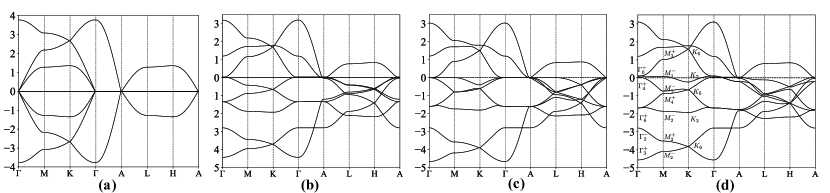
Figure S10: TB band structures of $H_{2}(\bm{k})$. (a) The chiral symmetric limit in perfect-flat band case #1 discussed in this section, with 3 perfectly flat bands. (b) The flat band limit discussed in case #3, with one perfectly flat band. (c) The flat band limit discussed in case #4, where a flat band exists along $\Gamma$-$M$, $\Gamma$-$A$, and $A$-$L$ lines. The parameters are taken as $\mu_{d_{3}}=\mu_{d_{4}}=-0.8,-t_{d_{3}}^{NN}=t_{d_{4}}^{NN}=-t_{d_{3},d_{4}}^{NN}=0.2,t_{d_{4}}^{zNN}=0$ and others the same as in Table S9 (d) The fitted bands to DFT results, with one quasi-flat band near $E_{f}$. The IRREPs are marked for bands on the $k_{z}=0$ plane. The TB parameters for (d) are summarized in Table S9.

II.3.3 $H_{3}(k)$: $d_{z^{2}}$ of Fe and bonding states of honeycomb Ge

In this section, we consider the TB model of $d_{z^{2}}@3f$ and the $sp^{2}$ bonding state formed by $s@3g$. They form two EBRs, i.e., $A_{g}@3f$ and $A^{\prime}@3g$.

For $d_{z^{2}}$ and $s$ orbitals on kagome sites, the local coordinate system defined in Eq. S2.7, which only mixes the $\bm{x}$ and $\bm{y}$ axes, is the same as the global Cartesian coordinate system. Thus we start from the local coordinate system directly. Choose the TB basis as

$$\psi_{\text{loc}}=(b@3g,d_{z^{2}}@3f).$$ (S2.46)

Under this basis, the generators of SG 191 have the following matrix form (permutations):

$$D_{\text{loc}}(C_{6z})=\left(\begin{matrix}0&0&1\\ 1&0&0\\ 0&1&0\\ \end{matrix}\right)\oplus\left(\begin{matrix}0&0&1\\ 1&0&0\\ 0&1&0\\ \end{matrix}\right),\quad D_{\text{loc}}(C_{2,110})=\left(\begin{matrix}0&0&1\\ 0&1&0\\ 1&0&0\\ \end{matrix}\right)\oplus\left(\begin{matrix}0&0&1\\ 0&1&0\\ 1&0&0\\ \end{matrix}\right),\quad D_{\text{loc}}(P)=\bm{1}_{6}.$$ (S2.47)

The TRS in the NSOC setting is $D_{\text{loc}}(T)=\bm{1}_{6}$.

We construct the following 6-band TB model:

$$H_{3}(\bm{k}) =\left(\begin{matrix}H_{b}(\bm{k})&S_{b,d_{5}}(\bm{k})\\ h.c.&H_{d_{5}}(\bm{k})\\ \end{matrix}\right),$$ (S2.48)

$$H_{d_{5}}(\bm{k}) =\mu_{d_{5}}\bm{1}_{3}+t_{d_{5}}^{NN}H_{\text{kagome}}^{\text{inplane},z^{2}}(k_{1},k_{2}),$$

$$H_{b}(\bm{k}) =(\mu_{b}+2t_{b}^{zNN}\cos(k_{z}))\bm{1}_{3}+t_{b}^{NN}H_{\text{kagome}}^{\text{inplane},z^{2}}(k_{1},k_{2}),$$

$$S_{b,d_{5}}(\bm{k}) =2\cos(\frac{k_{3}}{2})\left(t_{b,d_{5}}^{NN}\bm{1}_{3}+t_{b,d_{5}}^{NNN}H_{\text{kagome}}^{\text{inplane},z^{2}}(k_{1},k_{2})\right),$$

$$H_{\text{kagome}}^{\text{inplane},z^{2}}(k_{1},k_{2}) =2\left(\begin{matrix}0&\cos(\frac{k_{2}}{2})&\cos(\frac{k_{1}+k_{2}}{2})\\ &0&\cos(\frac{k_{1}}{2})\\ c.c.&&0\\ \end{matrix}\right).$$

In the model, $\mu_{i=d_{5},b}$ is the onsite energy, $t_{i=d_{5},b}^{NN}$ is NN intra-kagome hopping, and $t_{b}^{zNN}$ is the $z$-directional hopping of bonding state, and $t_{b,d_{5}}^{NN},t_{b,d_{5}}^{NNN}$ are the NN and NNN inter-layer hoppings. As shown in Fig. S11(a), we fit these parameters to the dispersion in DFT. The values of the parameters are listed in Table S9.

The main reason to combine the bonding state of honeycomb Ge with $d_{z^{2}}$ is that the $d_{z^{2}}$ orbital weights on $k_{3}=0$ plane have a wide distribution from -4 to 4 eV as seen from the orbital projections of DFT in Fig. S7, and using $d_{z^{2}}$ orbital alone cannot faithfully reproduce this band structure. By combining with the bonding state, the band structure and orbital weights of $d_{z^{2}}$ can be fitted better, and the DOS of $d_{z^{2}}$ near $E_{f}$ is also reduced by the bonding state as more $d_{z^{2}}$ weights are introduced below $E_{f}$ (see Table S10).

However, if one is only interested in the low energy physics near $E_{f}$, it is more convenient to use $d_{z^{2}}$ only to build a simpler model, as the $d_{z^{2}}$ weights below $-2$ eV are far from $E_{f}$ and can be perturbed out. We then constructed a model for $d_{z^{2}}$ only:

$$H_{d_{5}}(\bm{k})=\left(\mu_{d_{5}}+2t_{d_{5}}^{zNN}\cos(k_{3})\right)\bm{1}_{3}+t_{d_{5}}^{NN}H_{\text{kagome}}^{\text{inplane},z^{2}}(k_{1},k_{2}).$$ (S2.49)

where $t_{d_{5}}^{zNN}$ is $z$-directional hopping. Remark that in the fitted combined model with bonding states in Eq. S2.48, the onsite energies of $d_{z^{2}}$ and bonding state are close and the hopping between them is also strong, thus the second-order perturbation can not be applied directly. We thus refit parameters for $H_{d_{5}}(\bm{k})$ directly. The fitting parameters are $\mu_{d_{5}}=0.54,t_{d_{5}}^{NN}=-0.23,t_{d_{5}}^{zNN}=0.8$, using which the dispersion of $d_{z^{2}}$ close to $E_{f}$ is recovered, as shown in Fig. S11(b).

Compared with the 6-band model in Eq. S2.48 (with bonding states), the simplified model of $d_{z^{2}}$ only in Eq. S2.49 has about twice the $d_{z^{2}}$ orbital weights near $E_{f}$ (see Table S10 and Table S11). The weight at $E_{f}$ in the 3-band model is also larger than the orbital weights in DFT. Thus the 3-band TB model cannot faithfully capture the wavefunctions of DFT near $E_{f}$, which will lead to larger Coulomb interaction in the band basis. To remedy this, one needs to renormalize the Coulomb interaction of $d_{z^{2}}$ to smaller values when using the 3-band model.

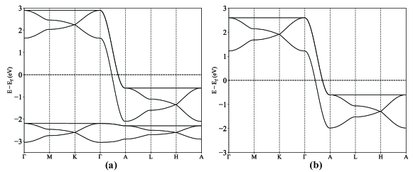
Figure S11: (a) Fitted TB band structure of $H_{3}(\bm{k})$ defined in Eq. S2.48. (b) Fitted TB band structure of $d_{z^{2}}$ only, defined in Eq. S2.49.

II.3.4 Full TB model

In this section, we first combine the three decoupled Hamiltonian $H_{1,2,3}$ together with an extra $S$-matrix between $p_{z}^{h}$ and $d_{2}$, and then use second-order perturbation theory to decouple the full Hamiltonian into three groups.

We combine the three models $H_{1,2,3}(\bm{k)}$ defined in Eq. S2.22, Eq. S2.37, Eq. S2.49 together, with the orbital basis

$$( p_{x}@1a,p_{y}@1a,d_{xy}@3f,d_{x^{2}-y^{2}}@3f)\oplus(p_{z}@2d,p_{z}@1a,d_{xz}@3f,d_{yz}@3f)\oplus(d_{z^{2}}@3f),$$ (S2.50)

which gives the full model:

$$H(\bm{k})=\left(\begin{array}[]{ccc|cccc|c}H_{p_{xy}^{t}}(\bm{k})&S_{p_{xy}^{t},d_{1}}(\bm{k})&S_{p_{xy}^{t},d_{2}}(\bm{k})&\underline{\bm{0}}&{\color[rgb]{1,0,0}\mathbf{0}}&{\color[rgb]{1,0,0}\mathbf{0}}&{\color[rgb]{1,0,0}\mathbf{0}}&\underline{\bm{0}}\\ &H_{d_{1}}(\bm{k})&S_{d_{1},d_{2}}(\bm{k})&{\color[rgb]{1,0,0}\mathbf{0}}&{\color[rgb]{1,0,0}\mathbf{0}}&{\color[rgb]{1,0,0}\mathbf{0}}&{\color[rgb]{1,0,0}\mathbf{0}}&\underline{\bm{0}}\\ &&H_{d_{2}}(\bm{k})&S_{p_{z}^{h},d_{2}}^{\dagger}(\bm{k})&{\color[rgb]{1,0,0}\mathbf{0}}&{\color[rgb]{1,0,0}\mathbf{0}}&{\color[rgb]{1,0,0}\mathbf{0}}&\underline{\bm{0}}\\ \hline\cr&&&H_{p_{z}^{h}}(\bm{k})&\underline{\bm{0}}&{\color[rgb]{1,0,0}\mathbf{0}}&S_{p_{z}^{h},d_{4}}(\bm{k})&\underline{\bm{0}}\\ &&&&H_{p_{z}^{t}}(\mathbf{k})&S_{p_{z}^{t},d_{3}}(\bm{k})&{\color[rgb]{1,0,0}\mathbf{0}}&{\color[rgb]{1,0,0}\mathbf{0}}\\ &&&&&H_{d_{3}}(\bm{k})&S_{d_{3},d_{4}}(\bm{k})&{\color[rgb]{1,0,0}\mathbf{0}}\\ &&&&&&H_{d_{4}}(\bm{k})&{\color[rgb]{1,0,0}\mathbf{0}}\\ \hline\cr h.c.&&&&&&&H_{d_{5}}(\bm{k})\\ \end{array}\right),$$ (S2.51)

where $p_{i}^{t}$ ($p_{i}^{h}$) denotes the $p_{i}$ orbitals of trigonal (honeycomb) Ge, and $d_{1}$ to $d_{5}$ denote $d_{xy},d_{x^{2}-y^{2}},d_{xz},d_{yz},d_{z^{2}}$, on kagome sites, respectively. The ${\color[rgb]{1,0,0}\mathbf{0}}$ in red means the NN coupling is forbidden by symmetries, and $\underline{\bm{0}}$ in black means the coupling has negligible values or is unimportant for fitting bands near the Fermi level.

The $S$-matrix of NN hopping between $p_{z}^{h}$ of honeycomb Ge and $d_{x^{2}-y^{2}}$ of kagome Fe is defined in Eq. S2.28. Similar to the $S_{p_{z}^{h},d_{4}}(\bm{k})$, $S_{p_{z}^{h},d_{2}}(\bm{k})=\mathbf{0}$ when $k_{3}=0$, and has rank 1 along the $k_{3}$ axis. This $S$-matrix brings $k_{3}$ dependence to $H_{1}(\bm{k})$, and the perfect flat band in Case (4) (see Sec.II.3.1) will not be perfectly flat on $k_{3}=\pi$ plane when $t_{p_{z}^{h},d_{2}}^{NN}\neq 0$. The coupling between $d_{2}$ and $p_{z}^{h}$ causes a band inversion at $L$ near the Fermi level for $d_{2}$ bands, which agrees with the IRREPs of DFT bands. The onsite energy difference of $p_{z}^{h}$ and $d_{x^{2}-y^{2}}$ is about $3$ eV, which justifies that excluding the $p_{z}^{h}$ orbital in $H_{1}(\bm{k})$ is reasonable as $p_{z}^{h}$ only slightly modifies the bands on $k_{3}=\pi$ plane. Remark that the orbitals in $H_{1}(\mathbf{k})$ mainly distribute on $xy$ plane, thus are quasi-2D and have weak $k_{3}$-dependence. However, the $d_{xy/yz}$ orbitals in $H_{2}(\mathbf{k})$ are mainly $z$-directional and naturally have strong $k_{3}$-dependence.

In the following, we use the second-order perturbation theory to decouple the combined model in order to obtain three simple decoupled Hamiltonians. As the onsite energy differences of $p_{z}^{h}$ orbitals and $d_{2}$ orbitals are large, we use the second-order perturbation method to decouple these orbitals. The perturbed Hamiltonians have the following form

$$H_{d_{2},p_{z}^{h}}^{(2)}(\bm{k}) =\frac{1}{\mu_{d_{2}}-\mu_{p_{z}^{h}}}S^{\dagger}_{p_{z}^{h},d_{2}}(\bm{k})S_{p_{z}^{h},d_{2}}(\bm{k})$$ (S2.52)

$$=\frac{(t_{p_{z}^{h},d_{2}}^{NN})^{2}}{\mu_{d_{2}}-\mu_{p_{z}^{h}}}\cdot 4\left((1-\cos(k_{3}))\mathbf{1}_{3}+(1-\cos(k_{3}))\left(\begin{matrix}0&\cos(\frac{k_{2}}{2})&\cos(\frac{k_{1}+k_{2}}{2})\\ &0&\cos(\frac{k_{1}}{2})\\ c.c.&&0\\ \end{matrix}\right)\right),$$

$$H_{p_{z}^{h},d_{2}}^{(2)}(\bm{k}) =\frac{1}{\mu_{p_{z}^{h}}-\mu_{d_{2}}}S_{p_{z}^{h},d_{2}}(\bm{k})S^{\dagger}_{p_{z}^{h},d_{2}}(\bm{k})$$

The onsite energy difference of $p_{z}^{t}$ and $d_{3}$ is also large, and they can be decoupled using similar second-order perturbation, with perturbed Hamiltonians:

$$H_{d_{3},p_{z}^{t}}^{(2)}(\bm{k}) =\frac{1}{\mu_{d_{3}}-\mu_{p_{z}^{t}}}S^{\dagger}_{p_{z}^{t},d_{3}}(\bm{k})S_{p_{z}^{t},d_{3}}(\bm{k})$$ (S2.53)

$$=\frac{2(t_{p_{z}^{t},d_{3}}^{NN})^{2}}{\mu_{d_{3}}-\mu_{p_{z}^{t}}}\left(\begin{matrix}1-\cos(k_{1})&2\sin(\frac{k_{1}}{2})\sin(\frac{k_{1}+k_{2}}{2})&2\sin(\frac{k_{1}}{2})\sin(\frac{k_{2}}{2})\\ &1-\cos(k_{1}+k_{2})&2\sin(\frac{k_{2}}{2})\sin(\frac{k_{1}+k_{2}}{2})\\ c.c.&&1-\cos(k_{2})\\ \end{matrix}\right),$$

We remark that the $p_{x,y}^{t}$ orbitals in $H_{1}(\mathbf{k})$ cannot be decoupled using second-order perturbation, as they have close onsite energies and strong coupling with $d_{1},d_{2}$ thus fail to meet the condition for 2nd-order perturbation to work (i.e., $\mu_{d}-\mu_{p}\gg t_{pd}$), and the perturbed band structure will change significantly. The honeycomb $p_{z}^{h}$ in $H_{2}(\mathbf{k})$ is similar. Moreover, these second-order perturbation formulas only apply rigorously when $H_{d_{i}}(\bm{k})$ and $H_{p_{z}^{h}}(\bm{k})$ are diagonal (see (see Appendix VIII)). When they are not diagonal, one can still do the numerical perturbation at each $k$-point but the perturbed Hamiltonians do not have a simple analytic form in the BZ. However, when $H_{d_{i}}(\bm{k})$ and $H_{p_{z}^{h}}(\bm{k})$ deviate not too large from the diagonal form, the 2nd-order perturbation formulas can be used as an approximation.

Using the aforementioned perturbed Hamiltonians, the full model is decoupled into the three following Hamiltonians

$$H_{1}(\bm{k}) =\left(\begin{matrix}H_{p_{xy}^{t}}(\bm{k})&S_{p_{xy}^{t},d_{1}}(\bm{k})&S_{p_{xy}^{t},d_{2}}(\bm{k})\\ &H_{d_{1}}(\bm{k})&S_{d_{1},d_{2}}(\bm{k})\\ h.c.&&H_{d_{2}}(\bm{k})+H_{d_{2},p_{z}^{h}}^{(2)}(\bm{k})\\ \end{matrix}\right),$$ (S2.54)

$$H_{2}(\bm{k}) =\left(\begin{matrix}H_{p_{z}^{h}}(\bm{k})+H_{p_{z}^{h},d_{2}}^{(2)}(\bm{k})&\bm{0}&S_{p_{z}^{h},d_{4}}(\bm{k})\\ &H_{d_{3}}(\bm{k})+H_{d_{3},p_{z}^{t}}^{(2)}(\bm{k})&S_{d_{3},d_{4}}(\bm{k})\\ h.c.&&H_{d_{4}}(\bm{k})\\ \end{matrix}\right),$$

$$H_{3}(\bm{k}) =H_{d_{5}}(\bm{k})$$

where $H_{i=1,2,3}(\mathbf{k})$ are defined in Eq. S2.22, Eq. S2.37, Eq. S2.49, with second-order perturbed terms defined in Eq. S2.52, Eq. S2.53. By direct-summing these three Hamiltonians, we arrive at

$$H(\bm{k})=H_{1}(\bm{k})\oplus H_{2}(\bm{k})\oplus H_{3}(\bm{k}),$$ (S2.55)

which gives the final decoupled single-particle Hamiltonian

$$\hat{H}_{0}=\sum_{\bm{k}}\sum_{ij}H_{ij}(\bm{k})c^{\dagger}_{\bm{k}i}c_{\bm{k}j},$$ (S2.56)

where the Bloch electron operators $c_{\bm{k}i}$ are defined as the Fourier transform of the following orbital basis

$$( p_{x}@1a,p_{y}@1a,d_{xy}@3f,d_{x^{2}-y^{2}}@3f)\oplus(p_{z}^{h}@2d,d_{xz}@3f,d_{yz}@3f)\oplus(d_{z^{2}}@3f),$$ (S2.57)

with orbitals defined in the local coordinate system in Eq. S2.7, and TB parameters values summarized in Table S9. The corresponding band structure is shown in Fig. S12. The filling number of each orbital and the DOS at $E_{f}$ in the decoupled model is given in Table S10, where most of the values agree well DFT (see Table S11) The largest error comes from the filling of $d_{x^{2}-y^{2}}$, which is smaller than the DFT value. This is due to a larger weight of $d_{x^{2}-y^{2}}$ above $E_{f}$ compared with DFT. The $d_{z^{2}}$ filling in the simplified $H_{3}(\mathbf{k})$ is also small compared with the DFT value. The $d_{z^{2}}$ filling becomes 1.55 when the bonding state is included which agrees well with DFT. We also list the filling within $[-1.5,1.5]$ eV, which shows better agreement with DFT with the root-mean-square error of $d$ orbitals fillings being $18\%$. Thus the model captures the low energy physics near $E_{f}$.

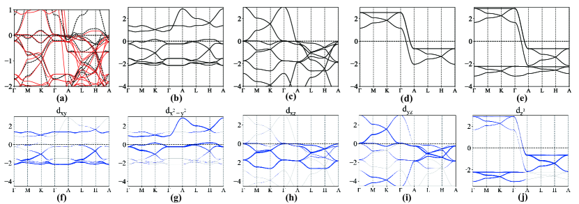
Figure S12: (a) Band structure of the direct-summed decoupled model in Eq. S2.55 (red lines), with a comparison with DFT bands in the PM phase (black dashed lines). (b)-(d) Band structure of the decoupled $H_{1}(\bm{k})$, $H_{2}(\bm{k})$, $H_{3}(\bm{k})$ defined in Eq. S2.54, respectively. (e) Band structure of $H_{3}(\bm{k})$ with bonding states defined in Eq. S2.48. (e)-(i) The orbital projection of each $d$ orbital in three decoupled models, where (i) shows the $d_{z^{2}}$ projections in $H_{3}(\bm{k})$ with bonding states. The orbital projections agree well with DFT results in S7.

Parameter	$\mu_{p_{xy}^{t}}$	$\mu_{d_{1}}$	$\mu_{d_{2}}$	$t_{d_{1}}^{NN}$	$t_{d_{2}}^{NN}$	$t_{d_{2}}^{NNN}$	$t_{d_{1},d_{2}}^{NN}$	$t_{d_{1},d_{2}}^{NNN}$	$t_{p_{xy}^{t},d_{1}}^{NN}$	$t_{p_{xy}^{t},d_{1}}^{NNN}$	$t_{p_{xy}^{t},d_{2}}^{NN}$	$t_{d}^{4N1}$	$t_{d}^{4N2}$	$t_{d}^{4N3}$
Value	-1.53	-0.96	0.06	0.58	0.11	0.09	-0.09	0.19	-0.33	0.14	0.35	-0.16	0.09	0.10
Parameter	$\mu_{p_{z}^{h}}$	$\mu_{d_{3}}$	$\mu_{d_{4}}$	$t_{d_{3},d_{4}}^{NN}$	$t_{d_{3}}^{NN}$	$t_{d_{4}}^{NN}$	$t_{d_{4}}^{zNN}$	$t_{p_{z}^{h},d_{4}}^{NN}$	$t_{p_{z}^{h}}^{NN}$	$t_{p_{z}^{h},d_{2}}^{NN}$	$\mu_{p_{z}^{t}}$	$t_{p_{z}^{t}}^{NN}$	$t_{p_{z}^{t},d_{3}}^{NN}$
Value	-1.47	-0.94	-0.89	-0.20	-0.23	0.2	0.10	0.77	-0.46	0.35	0.54	0.30	0.45
Parameter	$\mu_{d_{5}}$	$t_{d_{5}}^{NN}$	$\mu_{b}$	$t_{b}^{NN}$	$t_{b}^{zNN}$	$t_{b,d_{5}}^{NN}$	$t_{b,d_{5}}^{NNN}$
Value	-1.16	-0.25	-0.66	-0.1	0.9	-1.1	0.04

Table S9: Onsite energies and hoppings used in the full TB model (with bonding state in $H_{3}(\mathbf{k})$ defined in Eq. S2.48), where $d_{1}$ to $d_{5}$ denote $d_{xy},d_{x^{2}-y^{2}},d_{xz},d_{yz},d_{z^{2}}$, respectively, $p_{i}^{t}$ ($p_{i}^{h}$) denotes the $p_{i}$ orbitals of the trigonal (honeycomb) Ge, and $b$ is the $sp^{2}$ bonding state of honeycomb Ge. For the simplified $H_{3}(\mathbf{k})$ of $d_{z^{2}}$ only defined in Eq. S2.49, the parameters are $\mu_{d_{5}}=0.60,t_{d_{5}}^{NN}=-0.23,t_{d_{5}}^{zNN}=0.8$. Parameters not listed in the table have zero values.

Orbital	$p_{xy}^{t}$	$p_{z}^{h}$	$d_{z^{2}}$	$d_{xz}$	$d_{yz}$	$d_{x^{2}-y^{2}}$	$d_{xy}$	Total
TB filling $\in[-\infty,2]$	1.82	1.47	0.77	1.96	1.51	0.82	1.52	26.34
TB filling $\in[-1.5,1.5]$	0.05	0.18	0.69	1.22	0.98	0.76	0.43	12.72
TB DOS@$E_{f}$	0.00	0.02	0.14	0.08	0.21	0.44	0.06	1.00

Table S10: The filling and DOS at $E_{f}$ of each orbital in the decoupled TB model Eq. S2.55. The filling numbers are computed for bands $\in[-\infty,2]$ and $\in[-2,2]$ eV, averaged over atoms on the same Wyckoff positions, and time 2 to account for two degenerate spins. The DOS is normalized to 1. The filling in $[-2,2]$ eV agrees well with the DFT values in Table S4. The DOS at $E_{f}$ mainly comes from $d_{xz},d_{yz},d_{x^{2}-y^{2}}$ orbitals, which is also close to DFT results in Table S4. For the $H_{3}(\mathbf{k})$ with bonding state defined in Eq. S2.48, the $d_{z^{2}}$ filling in $[-\infty,2]$ is 1.55, in $[-2,2]$ is 0.46, and DOS$@E_{f}$ is 0.02 (not listed in the table for simplicity), which is more faithful as more $d_{z^{2}}$ weight below $E_{f}$ is introduced by the bonding states.

Orbital	$p_{xy}^{t}$	$p_{z}^{h}$	$d_{z^{2}}$	$d_{xz}$	$d_{yz}$	$d_{x^{2}-y^{2}}$	$d_{xy}$	Total
DFT filling $\in[-\infty,2]$	0.75	0.74	1.54	1.72	1.56	1.42	1.57	26.41
DFT filling $\in[-1.5,1.5]$	0.02	0.03	0.48	1.02	0.78	0.56	0.39	9.79
DFT DOS@$E_{f}$	0.00	0.00	0.02	0.21	0.31	0.33	0.06	0.94

Table S11: The filling and DOS$@E_{f}$ of each orbital computed using the Wannier TB model (can be seen as DFT values) constructed using $s,p,d$ orbitals of Fe and $s,p$ orbitals of Ge.

Appendix III Interaction parameters of FeGe

In this section, we compute the Coulomb interaction for FeGe using the ab initio constraint random phase approximation (cRPA) methodAryasetiawan et al. (2004); Solovyev and Imada (2005); Aryasetiawan et al. (2006); Miyake et al. (2009). We only compute the Coulomb interaction matrix for $d$ orbitals of Fe, as the Coulomb interactions of $s$ and $p$ orbitals of Fe and Ge have weaker interaction (for example, the intra-orbital onsite Hubbard $U$ for Ge $p$ is about two times smaller than that of Fe $d$, evaluated using the cRPA method to be introduced in the following), and the bands of them are also far away from $E_{f}$.

III.1 Constraint random phase approximation (cRPA) method

We first introduce the theoretical background of the cRPA method. In the cRPA method, one chooses a correlated subspace near the Fermi level that is usually generated by $3d$ (or $4f$) electrons. Because the $d$ (or $f$) orbitals in general have larger interactions than $p$ (or $s$) orbitals, one focuses on the interaction in the $d$-subspace. However, the $p$ orbitals always hybridize with $d$ orbitals in realistic materials which gives effective screening of the interaction of $d$ orbitals.

We start with the fully screened Coulomb interaction, which is given by

$$W(\bm{r},\bm{r}^{\prime};\omega)=\epsilon^{-1}(\bm{r},\bm{r}^{\prime};\omega)v(\bm{r},\bm{r}^{\prime}),$$ (S3.58)

where $v(\bm{r},\bm{r}^{\prime})$ is the bare Coulomb interaction, and $\epsilon(\bm{r},\bm{r}^{\prime};\omega)=1-v(\bm{r},\bm{r}^{\prime})P(\bm{r},\bm{r}^{\prime};\omega)$ is the dielectric function in RPA, with $P(\bm{r},\bm{r}^{\prime};\omega)$ being the non-interacting polarizationMiyake et al. (2009) given by:

$$P\left(\mathbf{r},\mathbf{r}^{\prime};\omega\right)=\sum_{\bm{k}n}^{\text{occ }}\sum_{\bm{k}^{\prime}n^{\prime}}^{\text{unocc }}\left\{\frac{\psi_{\bm{k}n}^{*}(\mathbf{r})\psi_{\bm{k}^{\prime}n^{\prime}}(\mathbf{r})\psi_{\bm{k}^{\prime}n^{\prime}}^{*}\left(\mathbf{r}^{\prime}\right)\psi_{\bm{k}n}\left(\mathbf{r}^{\prime}\right)}{\omega-\varepsilon_{\bm{k}^{\prime}n^{\prime}}+\varepsilon_{\bm{k}n}+i\delta}\right.\left.-\frac{\psi_{\bm{k}n}(\mathbf{r})\psi_{\bm{k}^{\prime}n^{\prime}}^{*}(\mathbf{r})\psi_{\bm{k}^{\prime}n^{\prime}}\left(\mathbf{r}^{\prime}\right)\psi_{\bm{k}n}^{*}\left(\mathbf{r}^{\prime}\right)}{\omega+\varepsilon_{\bm{k}^{\prime}n^{\prime}}-\varepsilon_{\bm{k}n}-i\delta}\right\},$$ (S3.59)

where $\psi_{\bm{k}n}$ and $\epsilon_{\bm{k}n}$ are single-particle eigenstates and eigenvalues, and ‘occ’ and ‘unocc’ denotes occupied and unoccupied states. For systems with narrow bands of $3d$ (or $4f$) orbitals, one could divide the polarization into two parts, i.e., $P(\bm{r},\bm{r}^{\prime};\omega)=P_{d}(\bm{r},\bm{r}^{\prime};\omega)+P_{r}(\bm{r},\bm{r}^{\prime};\omega)$, where $P_{d}(\bm{r},\bm{r}^{\prime};\omega)$ includes only $3d$ to $3d$ transitions, and $P_{r}(\bm{r},\bm{r}^{\prime};\omega)=P(\bm{r},\bm{r}^{\prime};\omega)-P_{d}(\bm{r},\bm{r}^{\prime};\omega)$ is the rest of the polarization. When the bands of $d$ orbitals are separated from other bands, $P_{d}(\bm{r},\bm{r}^{\prime};\omega)$ is computed by replacing the sum over all occupied and unoccupied states in Eq. S3.59 by the sum over the occupied and unoccupied states of $d$ orbitals only. However, when the bands of $d$ orbitals are entangled with other bands, $P_{d}(\bm{r},\bm{r}^{\prime};\omega)$ is not well-defined. Many methods are proposed in the literature to solve this problem, including the disentanglement methodMiyake et al. (2009) and the Projector methodKaltak (2015). The Projector method defines a projection operator that can extract the $d$ orbital contributions on each Bloch state and is the default method adopted in VASP, which we use in this work.

It was shownAryasetiawan et al. (2004); Solovyev and Imada (2005); Aryasetiawan et al. (2006); Miyake et al. (2009) that the partially screened Coulomb interaction of the electrons in the selected $d$ subspace is:

$$W_{r}(\bm{r},\bm{r}^{\prime};\omega)=\left[1-v(\bm{r},\bm{r}^{\prime})P_{r}(\bm{r},\bm{r}^{\prime};\omega)\right]^{-1}v(\bm{r},\bm{r}^{\prime}).$$ (S3.60)

Compared with the fully screened Coulomb interaction defined in Eq. S3.58, the partially screened interaction $W_{r}(\bm{r},\bm{r}^{\prime};\omega)$ is computed using the partial polarization $P_{r}(\bm{r},\bm{r}^{\prime};\omega)=P(\bm{r},\bm{r}^{\prime};\omega)-P_{d}(\bm{r},\bm{r}^{\prime};\omega)$, in which the contribution of $d-d$ screening has been removed from the total polarization. This subtraction could avoid the double counting of the $d-d$ screening since the $d-d$ screening is an inherent part of the $d$ subspace Hamiltonian and $W_{r}(\bm{r},\bm{r}^{\prime};\omega)$ can be interpreted as the effective interaction for electrons in the $d$-subspace. By combining Eq. S3.58 and Eq. S3.60, the fully screened interaction $W(\bm{r},\bm{r}^{\prime};\omega)$ can also be expressed by $W_{r}(\bm{r},\bm{r}^{\prime};\omega)$ as the result of further screening by $P_{d}(\bm{r},\bm{r}^{\prime};\omega)$:

$$W(\bm{r},\bm{r}^{\prime};\omega)=\left[1-W_{r}(\bm{r},\bm{r}^{\prime};\omega)P_{d}(\bm{r},\bm{r}^{\prime};\omega)\right]^{-1}W_{r}(\bm{r},\bm{r}^{\prime};\omega)$$ (S3.61)

Among the bare, partially screened, and fully screened Coulomb interactions, the bare Coulomb interaction $v(\bm{r},\bm{r}^{\prime})$ has the largest value while fully screened $W(\bm{r},\bm{r}^{\prime};\omega)$ has the smallest value, which means the more screening considered, the smaller the Coulomb interaction is for a given system.

With $W_{r}(\bm{r},\bm{r}^{\prime};\omega)$, the Coulomb interaction matrix can be evaluated using a localized basis set of the $d$ subspace, e.g., the maximally localized Wanneir functions $\{\varphi_{i}(\bm{r})\}$:

$$U_{ijkl}\left(\omega\right)=\iint d^{3}rd^{3}r^{\prime}\varphi_{i}^{*}(\mathbf{r})\varphi_{j}(\mathbf{r})W_{r}\left(\mathbf{r},\mathbf{r}^{\prime};\omega\right)\varphi_{k}^{*}\left(\mathbf{r}^{\prime}\right)\varphi_{l}\left(\mathbf{r}^{\prime}\right).$$ (S3.62)

Remark that the subscript convention follows the one used in VASP, and is different from the more commonly used convention of the Coulomb matrix (see Eq. S3.66). The computed interaction parameter values depend on the choice of Wannier functions. For basis with more orbitals, the Wannier functions are more localized in general, which produce larger U values.

In the Coulomb matrix, the following matrix elements are useful:

$$U_{iijj}(\omega) =\iint d^{3}rd^{3}r^{\prime}\left|\varphi_{i\mathbf{0}}(\mathbf{r})\right|^{2}W_{r}\left(\mathbf{r},\mathbf{r}^{\prime};\omega\right)\left|\varphi_{j\mathbf{0}}\left(\mathbf{r}^{\prime}\right)\right|^{2},$$ (S3.63)

$$U_{ijji}(\omega) =\iint d^{3}rd^{3}r^{\prime}\varphi_{i\mathbf{0}}^{*}(\mathbf{r})\varphi_{j\mathbf{0}}(\mathbf{r})W_{r}\left(\mathbf{r},\mathbf{r}^{\prime};\omega\right)\varphi_{j\mathbf{0}}^{*}\left(\mathbf{r}^{\prime}\right)\varphi_{i\mathbf{0}}\left(\mathbf{r}^{\prime}\right),$$

$$U_{ijij}(\omega) =\iint d^{3}rd^{3}r^{\prime}\varphi_{i\mathbf{0}}^{*}(\mathbf{r})\varphi_{j\mathbf{0}}(\mathbf{r})W_{r}\left(\mathbf{r},\mathbf{r}^{\prime};\omega\right)\varphi_{i\mathbf{0}}^{*}\left(\mathbf{r}^{\prime}\right)\varphi_{j\mathbf{0}}\left(\mathbf{r}^{\prime}\right),$$

where $U_{iijj}=:U_{ij}$ is the onsite (inter-orbital) Hubbard $U$, and $U_{ijji}=:J_{ij}$ is the onsite exchange (assume $i,j$ is the index of orbitals on the same site). $U_{ijji}=U_{ijij}$ if the basis $\{\varphi_{i}\}$ are real, which holds in spinless systems with TRS symmetry. FeGe in the PM phase has TRS symmetry, enforcing its Wannier functions to be real in the spinless setting, and thus $U_{ijji}=U_{ijij}$.

Using the Coulomb matrix elements, the Hubbard-Kanamori parameters are defined as

$$\mathcal{U} =\frac{1}{N}\sum_{i\in\mathcal{T}}U_{iiii}$$ (S3.64)

$$\mathcal{U}^{\prime} =\frac{1}{N(N-1)}\sum_{i,j\in\mathcal{T},i\neq j}^{N}U_{iijj}$$

$$\mathcal{J} =\frac{1}{N(N-1)}\sum_{i,j\in\mathcal{T},i\neq j}^{N}U_{ijji}$$

where $N$ is the number of orbitals in the target $d$ subspace. For cubic systems, $\mathcal{U}^{\prime}=\mathcal{U}-2\mathcal{J}$.

The general Coulomb interaction in real space is

$$\hat{H}_{\text{int}}=\frac{1}{2}\sum_{i,\sigma\sigma^{\prime}}\left\langle i_{1},i_{2}|W_{r}|i_{4},i_{3}\right\rangle c_{i_{1}\sigma}^{\dagger}c_{i_{2}\sigma^{\prime}}^{\dagger}c_{i_{3}\sigma^{\prime}}c_{i_{4}\sigma},$$ (S3.65)

where $i$ is a composite index denoting both sites and orbitals, and

$$\left\langle i_{1},i_{2}|W_{r}|i_{4},i_{3}\right\rangle =\iint d^{3}rd^{3}r^{\prime}\varphi_{i_{1}}^{*}(\mathbf{r})\varphi_{i_{2}}^{*}\left(\mathbf{r}^{\prime}\right)W_{r}\left(\mathbf{r},\mathbf{r}^{\prime}\right)\varphi_{i_{4}}\left(\mathbf{r}\right)\varphi_{i_{3}}(\mathbf{r}^{\prime})$$ (S3.66)

$$=\iint d^{3}rd^{3}r^{\prime}\varphi_{i_{1}}^{*}(\mathbf{r})\varphi_{i_{4}}\left(\mathbf{r}\right)W_{r}\left(\mathbf{r},\mathbf{r}^{\prime}\right)\varphi_{i_{2}}^{*}\left(\mathbf{r}^{\prime}\right)\varphi_{i_{3}}(\mathbf{r}^{\prime})$$

$$=U_{i_{1}i_{4}i_{2}i_{3}}$$

The interacting Hamiltonian can be simplified into the generalized Kanamori formGeorges et al. (2013) by considering the following onsite interactions

$$\hat{H}_{\text{int}} =\mathcal{U}\sum_{im}n_{im\uparrow}n_{im\downarrow}+\mathcal{U}^{\prime}\sum_{i,m\neq m^{\prime}}n_{im\uparrow}n_{im^{\prime}\downarrow}+(\mathcal{U}^{\prime}-\mathcal{J})\sum_{i,m<m^{\prime}\sigma}n_{im\sigma}n_{im^{\prime}\sigma}$$ (S3.67)

$$-\mathcal{J}_{X}\sum_{i,m<m^{\prime}}(c_{im\uparrow}^{\dagger}c_{im\downarrow}c_{im^{\prime}\downarrow}^{\dagger}c_{im^{\prime}\uparrow}+h.c.)+\mathcal{J}_{P}\sum_{i,m<m^{\prime}}(c_{im\uparrow}^{\dagger}c_{im\downarrow}^{\dagger}c_{im^{\prime}\downarrow}c_{im^{\prime}\uparrow}+h.c.)$$

where $i,j$ denote the different lattice sites, and $m,m^{\prime}$ denote different orbitals on the same site, i.e., we only consider the interaction between different orbitals on the same site. The $\mathcal{J}_{X}$ term is the spin-flipping term and the $\mathcal{J}_{P}$ term is the pair-hopping term. The Coulomb matrix element $U_{ijkl}=\left\langle i,k|W_{r}|l,j\right\rangle$, which is the coefficient of the two-body operator $c_{i\sigma}^{\dagger}c_{k\sigma^{\prime}}^{\dagger}c_{l\sigma^{\prime}}c_{j\sigma}$. Thus

• $U_{iijj}$ corresponds to $n_{i\sigma}n_{j\sigma^{\prime}}$ ($\mathcal{U},\mathcal{U}^{\prime}$).

• $U_{ijji}$ corresponds to $-c_{i\sigma}^{\dagger}c_{i\sigma^{\prime}}c_{j\sigma^{\prime}}^{\dagger}c_{j\sigma}$ ($\mathcal{J}_{X}$ if $\sigma=-\sigma^{\prime}$, $\mathcal{J}$ if $\sigma=\sigma^{\prime}$).

• $U_{ijij}$ corresponds to $c_{i\sigma}^{\dagger}c_{i\bar{\sigma}}^{\dagger}c_{j\bar{\sigma}}c_{j\sigma}$ ($\mathcal{J}_{P}$).

In the case of real Wannier basis, $\mathcal{J}=\mathcal{J}_{X}=\mathcal{J}_{P}$, and the Kanamori Hamiltonian has the simplified form

$$\hat{H}_{\text{int}} =\mathcal{U}\sum_{im}n_{im\uparrow}n_{im\downarrow}+\mathcal{U}^{\prime}\sum_{i,m\neq m^{\prime}}n_{im\uparrow}n_{im^{\prime}\downarrow}+(\mathcal{U}^{\prime}-\mathcal{J})\sum_{i,m<m^{\prime}\sigma}n_{im\sigma}n_{im^{\prime}\sigma}$$ (S3.68)

$$-\mathcal{J}\sum_{i,m\neq m^{\prime}}c_{im\uparrow}^{\dagger}c_{im\downarrow}c_{im^{\prime}\downarrow}^{\dagger}c_{im^{\prime}\uparrow}+\mathcal{J}\sum_{i,m\neq m^{\prime}}c_{im\uparrow}^{\dagger}c_{im\downarrow}^{\dagger}c_{im^{\prime}\downarrow}c_{im^{\prime}\uparrow}$$

If one considers orbital-dependent onsite interactions $U_{mm^{\prime}}$ and $J_{mm^{\prime}}$, the interacting Hamiltonian is generalized to

$$\hat{H}_{\text{int}} =\sum_{im}U_{mm}n_{im\uparrow}n_{im\downarrow}+\sum_{i,m\neq m^{\prime}}U_{mm^{\prime}}n_{im\uparrow}n_{im^{\prime}\downarrow}+\sum_{i,m<m^{\prime}\sigma}(U_{mm^{\prime}}-J_{mm^{\prime}})n_{im\sigma}n_{im^{\prime}\sigma}$$ (S3.69)

$$-\sum_{i,m\neq m^{\prime}}J_{mm^{\prime}}c_{im\uparrow}^{\dagger}c_{im\downarrow}c_{im^{\prime}\downarrow}^{\dagger}c_{im^{\prime}\uparrow}+\sum_{i,m\neq m^{\prime}}J_{mm^{\prime}}c_{im\uparrow}^{\dagger}c_{im\downarrow}^{\dagger}c_{im^{\prime}\downarrow}c_{im^{\prime}\uparrow}$$

In the following, we will use the cRPA method to compute $U_{ij}$ and $J_{ij}$ to obtain the interacting Hamiltonian for FeGe.

III.2 cRPA interactions parameters for FeGe

We compute the Coulomb interaction matrix using the cRPA method implemented in VASPKresse and Furthmüller (1996b); Kaltak (2015), where the partially screened Coulomb interaction kernel Eq. S3.60 is first computed, and Coulomb interaction is evaluated using a set of maximally localized Wannier functions (obtained from WANNIER90Mostofi et al. (2008)) based on Eq. S3.62.

We first construct MLWFs using $d$ orbitals of Fe and $p$ orbitals of Ge, which have 24 orbitals in total. Two models can be constructed from them. One is called the $d-dp$ model in the literatureVaugier et al. (2012), which excludes only the polarization inside the $d$ orbitals when computing the partially screened Coulomb interaction. The other model is called the $dp-dp$ modelVaugier et al. (2012), which excludes the polarization of both $d$ and $p$ orbitals. The $dp-dp$ model produces a larger Coulomb interaction as more screening is removed.

We also construct another set of MLWFs using $s,p,d$ orbitals of Fe and $s,p$ orbitals of Ge, which has 39 orbitals in total. The MLWFs are more localized as more orbitals are included. A third model, which we call $d-$full, is constructed based on this large MLWF set which screens only $d$ orbitals.

In Table S12, S13, and S14, we list the Coulomb interaction matrix $U_{ij}$ and $J_{ij}$ for the five $d$ orbitals on the same Fe, the NN and NNN Coulomb interaction $U_{ij}^{NN}$ and $U_{ij}^{NNN}$ of five $d$ orbitals, and the Hubbard-Kanamori parameters computed for five $d$ orbitals on the same site for the $d-dp$, $dp-dp$, and $d$-full model, respectively.

For the three models, $d-dp$ and $d$-full models have comparable interaction values and can be used in interacting Hamiltonians with compatible Wannier basis sets. The $dp-dp$ model, however, has significantly larger interaction values compared with $d-dp$ and $d$-full models, and can only be used in the interacting Hamiltonians where both $d$ and $p$ orbitals have interactions.

$U_{ij}$	$z^{2}$	$xz$	$yz$	$x^{2}-y^{2}$	$xy$		$J_{ij}$	$z^{2}$	$xz$	$yz$	$x^{2}-y^{2}$	$xy$
$z^{2}$	3.81	2.87	2.93	2.41	2.41				0.47	0.50	0.75	0.73
$xz$		3.81	2.57	2.59	2.58					0.68	0.67	0.65
$yz$			4.06	2.64	2.64						0.70	0.67
$x^{2}-y^{2}$				4.04	3.2							0.40
$xy$					3.96
$U_{ij}^{NN}$	$z^{2}$	$xz$	$yz$	$x^{2}-y^{2}$	$xy$		$U_{ij}^{NNN}$	$z^{2}$	$xz$	$yz$	$x^{2}-y^{2}$	$xy$
$z^{2}$	1.48	1.47	1.48	1.50	1.51			1.27	1.27	1.26	1.27	1.27
$xz$		1.48	1.48	1.50	1.51				1.27	1.26	1.28	1.28
$yz$			1.50	1.52	1.52					1.26	1.27	1.27
$x^{2}-y^{2}$				1.55	1.56						1.28	1.29
$xy$					1.58							1.29

Table S12: The Coulomb interaction $U_{ij}$ and $J_{ij}$ of $d$ orbitals, and $U_{ij}^{NN}$ and $U_{ij}^{NNN}$ between NN and NNN $d$ orbitals in $d-dp$ model. where $U_{ij}=U_{iijj}$ and $J_{ij}=U_{ijji}$, with $U_{ijkl}$ defined in Eq. S3.63. The onsite Hubbard-Kanamori parameters are $\mathcal{U}=3.94,\mathcal{U}^{\prime}=2.69,\mathcal{J}=0.62$. All numbers are in eV.

$U_{ij}$	$z^{2}$	$xz$	$yz$	$x^{2}-y^{2}$	$xy$		$J_{ij}$	$z^{2}$	$xz$	$yz$	$x^{2}-y^{2}$	$xy$
$z^{2}$	8.00	7.15	7.21	6.55	6.44				0.49	0.52	0.83	0.79
$xz$		8.25	6.89	6.88	6.74					0.74	0.72	0.71
$yz$			8.51	6.91	6.81						0.77	0.73
$x^{2}-y^{2}$				8.39	7.41							0.40
$xy$					8.05
$U_{ij}^{NN}$	$z^{2}$	$xz$	$yz$	$x^{2}-y^{2}$	$xy$		$U_{ij}^{NNN}$	$z^{2}$	$xz$	$yz$	$x^{2}-y^{2}$	$xy$
$z^{2}$	2.68	2.67	2.69	2.72	2.73			1.87	1.88	1.86	1.88	1.88
$xz$		2.67	2.68	2.71	2.72				1.89	1.87	1.89	1.90
$yz$			2.71	2.74	2.75					1.86	1.88	1.88
$x^{2}-y^{2}$				2.78	2.79						1.90	1.90
$xy$					2.81							1.91

Table S13: The Coulomb interaction $U_{ij}$ and $J_{ij}$ of $d$ orbitals, and $U_{ij}^{NN}$ and $U_{ij}^{NNN}$ between NN and NNN $d$ in $dp-dp$ model. The onsite Hubbard-Kanamori parameters are $\mathcal{U}=8.24,\mathcal{U}^{\prime}=6.90,\mathcal{J}=0.67$. All numbers are in eV.

$U_{ij}$	$z^{2}$	$xz$	$yz$	$x^{2}-y^{2}$	$xy$		$J_{ij}$	$z^{2}$	$xz$	$yz$	$x^{2}-y^{2}$	$xy$
$z^{2}$	4.16	2.87	3.04	2.42	2.45				0.54	0.57	0.90	0.92
$xz$		3.80	2.51	2.53	2.57					0.74	0.74	0.76
$yz$			4.21	2.70	2.74						0.77	0.80
$x^{2}-y^{2}$				4.28	3.43							0.47
$xy$					4.46
$U_{ij}^{NN}$	$z^{2}$	$xz$	$yz$	$x^{2}-y^{2}$	$xy$		$U_{ij}^{NNN}$	$z^{2}$	$xz$	$yz$	$x^{2}-y^{2}$	$xy$
$z^{2}$	1.38	1.38	1.40	1.40	1.41			1.22	1.22	1.22	1.22	1.22
$xz$		1.39	1.39	1.40	1.40				1.22	1.22	1.23	1.23
$yz$			1.42	1.42	1.42					1.21	1.22	1.22
$x^{2}-y^{2}$				1.44	1.44						1.23	1.23
$xy$					1.45							1.23

Table S14: The Coulomb interaction $U_{ij}$ and $J_{ij}$ of $d$ orbitals, and $U_{ij}^{NN}$ and $U_{ij}^{NNN}$ between NN and NNN $d$ in $d-$full model. The onsite Hubbard-Kanamori parameters are $\mathcal{U}=4.18,\mathcal{U}^{\prime}=2.73,\mathcal{J}=0.72$. These values satisfy the relation $\mathcal{U}^{\prime}\approx\mathcal{U}-2\mathcal{J}$ which holds exactly in cubic systems. The averaged NN and NNN interactions are $\bar{U}^{NN}=1.41,\bar{U}^{NNN}=1.22$. All numbers are in eV.

III.3 Approximated interaction parameters

In this section, we simplify the Coulomb interaction matrix via approximate symmetries.

In the $d$-full model shown in Table S14, the averaged onsite Hubbard-Kanamori parameters are $\mathcal{U}=4.18,\mathcal{U}^{\prime}=2.73,\mathcal{J}=0.72$ eV for five $d$ orbitals on the same site, as shown in Table S14. These values satisfy the relation $\mathcal{U}^{\prime}\approx\mathcal{U}-2\mathcal{J}$ which holds exactly in cubic systems. The Hubbard-Kanamori parameters are averaged values (defined in Eq. S3.64) and are thus symmetric for five $d$ orbitals, thus having $\text{SU}(2)$ spin-rotation symmetry and $\text{SO}(5)$ orbital symmetry.

However, the five $d$ orbitals are in fact symmetry-independent, as the site symmetry group of the kagome site is $D_{2h}$, which has no symmetry that could relate different $d$ orbitals. Thus the Coulomb interactions $U_{ij}$ and $J_{ij}$ of $d$ orbitals can take independent values and only have $\text{SU}(2)$ spin-rotation symmetry.

Although five $d$ orbitals are symmetry-independent, their interactions still share similarities, e.g., the onsite intra-orbital Hubbard $U_{ii}$ values are close, which indicates approximated symmetries. To simplify the Coulomb matrix, we will assume cubic and spherical symmetries in the following.

For the NN and NNN interactions $U_{ij}^{NN}$ and $U_{ij}^{NNN}$ in the $d$-full model, we adopt the spherical approximation and average them over orbitals:

$$\overline{U}^{NN} =\frac{1}{25}\sum_{ij}U_{ij}^{NN}=1.41\text{ eV}$$ (S3.70)

$$\overline{U}^{NNN} =\frac{1}{25}\sum_{ij}U_{ij}^{NNN}=1.22\text{ eV}$$

The root mean square error for $U_{ij}^{NN}$ and $U_{ij}^{NNN}$ is 0.019 and 0.004 eV, respectively.

For the onsite Coulomb matrix, we will first assume cubic symmetries and compute the symmetrized values, and then further assume spherical symmetries and adopt the Slater integrals to evaluate the approximated Coulomb matrix, as shown in the following sections.

III.3.1 Symmetrized Coulomb matrix using $O_{h}$ symmetries

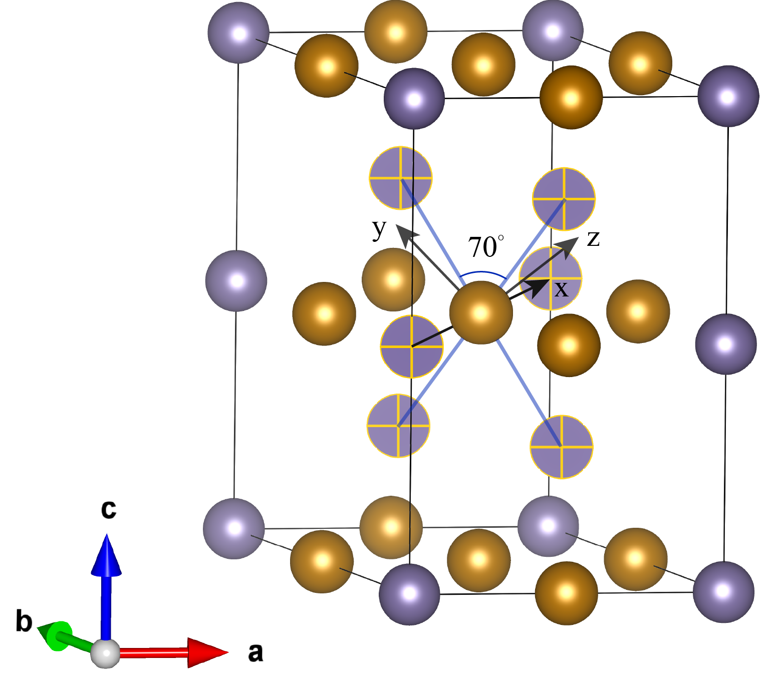
Figure S13: Schematic show of the quasi-cubic local coordinate system for Fe atom at $(\frac{1}{2},\frac{1}{2},\frac{1}{2})$, defined in Eq. S3.71. Each Fe atom has six closest surrounding Ge atoms that form a distorted octahedron and thus give an approximated cubic crystal field.

The assumption of cubic symmetries can be justified using the following local coordinate, as shown in Fig. S13. For each Fe atom on the kagome site in FeGe, there are six nearest Ge atoms, i.e., two trigonal Ge’s and four honeycomb Ge’s, which form a distorted octahedron and give an approximated cubic field. The local coordinate system is defined as

$$3f_{1} :\bm{x}_{1}=(1,0,0),\bm{y}_{1}=(0,\frac{1}{\sqrt{2}},\frac{1}{\sqrt{2}}),\bm{z}_{1}=(0,-\frac{1}{\sqrt{2}},\frac{1}{\sqrt{2}})$$ (S3.71)

$$3f_{2} :\bm{x}_{2}=(\frac{1}{2},\frac{\sqrt{3}}{2},0),\bm{y}_{2}=(-\frac{\sqrt{3}}{2\sqrt{2}},\frac{1}{2\sqrt{2}},\frac{1}{\sqrt{2}}),\bm{z}_{2}=(\frac{\sqrt{3}}{2\sqrt{2}},-\frac{1}{2\sqrt{2}},\frac{1}{\sqrt{2}})$$

$$3f_{3} :\bm{x}_{3}=(-\frac{1}{2},\frac{\sqrt{3}}{2},0),\bm{y}_{3}=(-\frac{\sqrt{3}}{2\sqrt{2}},-\frac{1}{2\sqrt{2}},\frac{1}{\sqrt{2}}),\bm{z}_{3}=(\frac{\sqrt{3}}{2\sqrt{2}},\frac{1}{2\sqrt{2}},\frac{1}{\sqrt{2}})$$

We call this local coordinate system the “quasi-cubic local coordinate system” as six neighboring Ge atoms form an approximated cubic field. We recompute the cRPA Coulomb matrix in the $d$-full model using the quasi-cubic local coordinate system, with $U_{ij}$ and $J_{ij}$ tabulated in Table S15. This Coulomb matrix is more symmetric, e.g., the intra-orbital Hubbard $U_{ii}$ of each $d$ orbital is more close to the averaged $\mathcal{U}$.

We remark that this quasi-cubic local environment only holds well by considering six neighboring Ge atoms for each Fe atom, while the inclusion of NN Fe atoms will spoil the cubic environment. Since in the cRPA calculations, only the $p$ (and s) orbitals of Ge are projected out while the $d-d$ screening of Fe is kept, this quasi-cubic local environment of Fe given by the Ge atoms can still approximately hold. In the single-particle Wannier TB model (see Table S5), the hopping parameters do not show good agreements with this cubic environment, possibly because both Fe and Ge contribute to the local environment in the TB and the $d$ orbitals in the TB are also not aligned with this cubic local coordinates.

The original onsite Coulomb matrix $U_{ijkl}^{o}$ in the $d$-full model (computed under basis $\psi^{\text{loc}}$ under local coordinates Eq. S2.7) is related to the onsite Coulomb matrix $U_{ijkl}^{c}$ computed using basis $\psi^{\text{quasi-cubic}}$ in the quasi-cubic local coordinate systems by the following transformation $S$, derived from the transformation $\psi^{\text{quasi-cubic}}_{i}=S_{ij}\psi_{j}^{\text{loc}}$

$$S =\left(\begin{matrix}\frac{1}{4}&0&-\frac{\sqrt{3}}{2}&-\frac{\sqrt{3}}{4}&0\\ 0&\frac{1}{\sqrt{2}}&0&0&-\frac{1}{\sqrt{2}}\\ \frac{\sqrt{3}}{2}&0&0&\frac{1}{2}&0\\ -\frac{\sqrt{3}}{4}&0&-\frac{1}{2}&\frac{3}{4}&0\\ 0&\frac{1}{\sqrt{2}}&0&0&\frac{1}{\sqrt{2}}\\ \end{matrix}\right),$$ (S3.72)

$$U^{c}_{ijkl}=\sum_{i^{\prime}j^{\prime}k^{\prime}l^{\prime}}S^{*}_{ii^{\prime}}S^{*}_{jj^{\prime}}U^{o}_{i^{\prime}j^{\prime}k^{\prime}l^{\prime}}S_{kk^{\prime}}S_{ll^{\prime}}$$ (S3.73)

$U_{ij}$	$z^{2}$	$xz$	$yz$	$x^{2}-y^{2}$	$xy$	$J_{ij}$	$z^{2}$	$xz$	$yz$	$x^{2}-y^{2}$	$xy$
$z^{2}$	4.18	3.03	3.11	2.40	2.40			0.56	0.57	0.88	0.87
$xz$		4.11	2.66	2.59	2.59				0.78	0.77	0.78
$yz$			4.33	2.65	2.66					0.79	0.78
$x^{2}-y^{2}$				4.13	3.21						0.45
$xy$					4.11

Table S15: The Coulomb interaction $U_{ij}$ and $J_{ij}$ in the quasi-cubic local coordinate system that aligned with the bonds between Fe and Ge, which form an approximated cubic lattice field.

We then further symmetrize the onsite Coulomb matrix $U_{ijkl}^{o}$ computed in the $d$-full model by assuming the cubic $O_{h}$ symmetry group. $O_{h}$ can be generated by the following three generators:

$$C_{3,111} =\left(\begin{matrix}0&0&1\\ 1&0&0\\ 0&1&0\\ \end{matrix}\right),\quad C_{4,z}=\left(\begin{matrix}0&-1&0\\ 1&0&0\\ 0&0&1\\ \end{matrix}\right),\quad P=\left(\begin{matrix}-1&0&0\\ 0&-1&0\\ 0&0&-1\\ \end{matrix}\right),$$ (S3.74)

which have representation matrices under five $d$ orbitals $(d_{z^{2}},d_{xz},d_{yz},d_{x^{2}-y^{2}},d_{xy})$:

$$D(C_{3,111}) =\left(\begin{matrix}-\frac{1}{2}&0&0&-\frac{\sqrt{3}}{2}&0\\ 0&0&1&0&0\\ 0&0&0&0&1\\ \frac{\sqrt{3}}{2}&0&0&-\frac{1}{2}&0\\ 0&1&0&0&0\\ \end{matrix}\right),\quad D(C_{4,z})=\left(\begin{matrix}1&0&0&0&0\\ 0&0&-1&0&0\\ 0&1&0&0&0\\ 0&0&0&-1&0\\ 0&0&0&0&-1\\ \end{matrix}\right),\quad D(P)=\left(\begin{matrix}1&0&0&0&0\\ 0&1&0&0&0\\ 0&0&1&0&0\\ 0&0&0&1&0\\ 0&0&0&0&1\\ \end{matrix}\right).$$ (S3.75)

where the transformation is defined as $d_{i}(g^{-1}\bm{r})=d_{j}(\bm{r})D_{ji}(g)$, or equivalently, $d_{i}(g\bm{r})=D_{ij}(g)d_{j}(\bm{r})$, as $D^{T}(g)=D^{-1}(g)=D(g^{-1})$.

Using these generators, we generate all 48 operations in the $O_{h}$ group and symmetrize the Coulomb matrix:

$$U^{\text{sym}}_{ijkl}=\frac{1}{N_{\mathcal{G}}}\sum_{g\in\mathcal{G}}\sum_{i^{\prime}j^{\prime}k^{\prime}l^{\prime}}D(g)^{*}_{ii^{\prime}}D(g)^{*}_{jj^{\prime}}U^{o}_{i^{\prime}j^{\prime}k^{\prime}l^{\prime}}D(g)_{kk^{\prime}}D(g)_{ll^{\prime}},$$ (S3.76)

where $\mathcal{G}=O_{h}$, $N_{\mathcal{G}}=48$, and $U_{ijkl}^{o}$ denote the original Coulomb matrix computed using the cRPA method. The symmetrized Coulomb matrix elements $U_{ij}$ and $J_{ij}$ for the $d$-full model are tabulated in Table S16. The onsite Hubbard $U$ values have $T_{2g}$ ($d_{xz},d_{yz},d_{xy}$) and $E_{g}$ ($d_{z^{2}},d_{x^{2}-y^{2}}$) splitting. We remark that in practice using $O$ group symmetries is equivalent for five $d$ orbitals, as $D(P)=\bm{1}_{5}$ which has no effects.

$U_{ij}$	$z^{2}$	$xz$	$yz$	$x^{2}-y^{2}$	$xy$	$J_{ij}$	$z^{2}$	$xz$	$yz$	$x^{2}-y^{2}$	$xy$
$z^{2}$	4.22	3.05	3.05	2.42	2.41			0.56	0.56	0.90	0.88
$xz$		4.16	2.61	2.62	2.61				0.77	0.78	0.77
$yz$			4.16	2.62	2.61					0.78	0.77
$x^{2}-y^{2}$				4.22	3.27						0.46
$xy$					4.16

Table S16: The onsite Coulomb interaction $U_{ij}$ and $J_{ij}$ of $d$ orbitals symmetrized using $O_{h}$ symmetries. The root mean square error of the symmetrized $U_{ij}$ and $J_{ij}$ to the original ones is 0.132 and 0.023, respectively.

III.3.2 Slater integrals

In Table S16, the onsite Coulomb matrix symmetrized by $O_{h}$ symmetries still has some matrix elements that take very close values, e.g., the five intra-orbital $U_{ii}$, which suggests a higher symmetry group, i.e., spherical $\text{SO}(3)$ rotation symmetry. For the spherical Coulomb matrix, Slater integralsSlater (1960); Sugano (2012) can be adopted to parameterize. We first give a brief introduction to the Slater integrals in this section and then fit the value of the Slater integrals in the next section.

The Coulomb matrix in a spherical lattice field can be parametrized by Slater integrals $F^{k}$ in the complex spherical harmonics basis with the formWang et al. (2015); Vaugier et al. (2012)

$$U_{m_{1},m_{2},m_{3},m_{4}}=\delta_{m_{1}+m_{2},m_{3}+m_{4}}\sum_{k}c_{k}^{m_{1},m_{3}}c_{k}^{m4,m2}F^{k},$$ (S3.77)

where $c_{k}^{m_{i},m_{j}}$ is the Gaunt coefficient, whose value is tabulated in Table 1.2 in Ref.Sugano (2012), and $F^{k}$ are Slater integrals that need to be fitted for specific materials. For $d$ orbitals, there are only three nonzero Slater integrals $F_{0}$, $F_{2}$, and $F_{4}$ as $l=2$ (for $f$ orbitals, $F_{6}$ is also needed), and it is a good approximation to take the average value $F_{4}=0.625F_{2}$ for $3d$ transition metals according to literaturede Groot et al. (1990); Anisimov et al. (1997).

For $3d$ shell, Eq. S3.77 is written in complex spherical harmonics basis $\phi_{l=2,m}(\bm{r})=R_{3d}(r)Y_{l=2}^{m}(\bm{r})$, and needs to be transformed to cubic harmonic basis $\psi_{m}(\bm{r})=R_{3d}(r)X_{2c}(\bm{r})$ which are used in Wannier functions, where the radical parts $R_{3d}(r)$ are identical while the angular parts $X_{2c}(\bm{r})$ are related to $Y_{2}^{m}$ by the following equations

$$d_{z^{2}} =N_{2}^{c}\frac{3z^{2}-r^{2}}{2r^{2}\sqrt{3}}=Y_{2}^{0}$$ (S3.78)

$$d_{xz} =N_{2}^{c}\frac{xz}{r^{2}}=\frac{1}{\sqrt{2}}(Y_{2}^{-1}-Y_{2}^{1})$$

$$d_{yz} =N_{2}^{c}\frac{yz}{r^{2}}=\frac{i}{\sqrt{2}}(Y_{2}^{-1}+Y_{2}^{1})$$

$$d_{xy} =N_{2}^{c}\frac{xy}{r^{2}}=\frac{i}{\sqrt{2}}(Y_{2}^{-2}-Y_{2}^{2})$$

$$d_{x^{2}-y^{2}} =N_{2}^{c}\frac{x^{2}-y^{2}}{2r^{2}}=\frac{1}{\sqrt{2}}(Y_{2}^{-2}+Y_{2}^{2})$$

The following relations can be derived for onsite Hubbard U and Hund’s exchange $J_{ij}$ of five $d$ orbitals for spherical-symmetric systems using Eq. S3.77 and the value of Gaunt coefficientsWang et al. (2015):

$$U =F^{0}+\frac{4}{49}(F^{2}+F^{4})$$ (S3.79)

$$J(d_{z^{2}},d_{xz}) =J(d_{z^{2}},d_{yz})=\frac{1}{49}F^{2}+\frac{30}{441}F^{4}$$

$$J(d_{z^{2}},d_{x^{2}-y^{2}}) =J(d_{z^{2}},d_{xy})=\frac{4}{49}F^{2}+\frac{15}{441}F^{4}$$

$$J(d_{xz},d_{yz}) =J(d_{xz},d_{x^{2}-y^{2}})=J(d_{xz},d_{xy})$$

$$=J(d_{yz},d_{x^{2}-y^{2}})=J(d_{yz},d_{xy})=\frac{3}{49}F^{2}+\frac{20}{441}F^{4}$$

$$J(d_{x^{2}-y^{2}},d_{xy}) =\frac{35}{441}F^{4}$$

III.3.3 Fitting Slater integrals

We fit the Slater integrals $F^{0},F^{2},F^{4}$ to the Coulomb matrix symmetrized using $O_{h}$ symmetries as well as the one computed in the quasi-cubic local coordinate system, which yields identical values of Slater integrals. The resultant Coulomb matrix computed from the Slater integrals is shown in Table S17. It has spherical symmetries and is invariant under any $\text{SO}(3)$ coordinate transformations. The ratio for the fitted parameters is $F^{4}/F^{2}=0.686$, which is close to $0.625$.

We also use the approximated relation $F^{4}=0.625F^{2}$ in literaturede Groot et al. (1990) and fit only the Slater integrals $F^{0}$ and $F^{2}$, with results shown in Table S18. The resultant Coulomb matrix has a slightly larger fitting error compared with Table S17, but only has two parameters $F^{0}$ and $F^{2}$, which is simpler for further mean-field calculations.

$U_{ij}$	$z^{2}$	$xz$	$yz$	$x^{2}-y^{2}$	$xy$	$J_{ij}$	$z^{2}$	$xz$	$yz$	$x^{2}-y^{2}$	$xy$
$z^{2}$	4.18	3.05	3.05	2.41	2.41			0.56	0.56	0.88	0.88
$xz$		4.18	2.62	2.62	2.62				0.78	0.78	0.78
$yz$			4.18	2.62	2.62					0.78	0.78
$x^{2}-y^{2}$				4.18	3.26						0.46
$xy$					4.18

Table S17: The Coulomb interaction $U_{ij}$ and $J_{ij}$ of $d$ orbitals fitted using Eq. S3.77, where the Slater integrals $F^{0}$, $F^{2}$, and $F^{4}$ are fitted to the full Coulomb matrix $U_{ijkl}$ computed using cRPA method in the quasi-cubic local coordinate system. The fitted parameters are $F^{0}=3.018,F^{2}=8.409,F^{4}=5.766$. The root mean square error (the error between the fitted values and the DFT values) of the fitted $U_{ij}$ and $J_{ij}$ is 0.133 and 0.024, respectively.

$U_{ij}$	$z^{2}$	$xz$	$yz$	$x^{2}-y^{2}$	$xy$	$J_{ij}$	$z^{2}$	$xz$	$yz$	$x^{2}-y^{2}$	$xy$
$z^{2}$	4.15	3.08	3.08	2.39	2.39			0.54	0.54	0.88	0.88
$xz$		4.15	2.62	2.62	2.62				0.77	0.77	0.77
$yz$			4.15	2.62	2.62					0.77	0.77
$x^{2}-y^{2}$				4.15	3.30						0.42
$xy$					4.15

Table S18: The Coulomb interaction $U_{ij}$ and $J_{ij}$ of $d$ orbitals fitted using Eq. S3.77, where the Slater integrals $F^{0}$, $F^{2}$ are fitted to the full Coulomb matrix $U_{ijkl}$ computed using cRPA method in the quasi-cubic local coordinate system, while $F^{4}=0.625F^{2}$ are fixed. The fitted parameters are $F^{0}=3.018,F^{2}=8.544,F^{4}=5.346$. The root mean square error of the fitted $U_{ij}$ and $J_{ij}$ is 0.134 and 0.028, respectively.

Appendix IV Summary of TB models and interaction parameters of FeGe

In this section, we give a brief summary of the TB models and interaction parameters in FeGe discussed in Appendix II and Appendix III.

To construct TB models for the complicated band structure of FeGe, we first choose three sets of orbitals, i.e., (i) $d_{x^{2}-y^{2}},d_{xy}$ of Fe and $p_{x},p_{y}$ of trigonal Ge, (ii) $d_{xz},d_{yz}$ of Fe and $p_{z}$ of honeycomb and trigonal Ge, and (iii) $d_{z^{2}}$ of Fe and the $sp^{2}$ bonding state of honeycomb Ge, and build TB models with NN and a few longer-range hoppings for them. The fitted TB models match the two quasi-flat bands and the van Hove singularities below the Fermi level. We then couple the three models together to construct the full model in Eq. S2.51. At last, we decouple them using second-order perturbations and obtain three independent models in Eq. S2.54, with hopping parameters listed in Table S9. The band structures of these models are shown in Fig. S12.

To compute the interaction parameters, we use the cRPA method implemented in VASP to obtain the screened Coulomb matrix using Wannier functions. In Table S12, S13, and S14, we list the onsite Coulomb interaction matrix elements $U_{ij}$, $J_{ij}$, as well as the NN and NNN Coulomb interactions $U_{ij}^{NN}$ and $U_{ij}^{NNN}$ for the so-called $d-dp$ model, $dp-dp$ model, and $d$-full models.

We take the Coulomb matrix in the $d$-full model and do further approximations. We take spherical approximations for Coulomb interactions that are not onsite, i.e., the NN and NNN Coulomb interactions $U_{ij}^{NN}$ and $U_{ij}^{NNN}$ are set to be equal, respectively. For the onsite Coulomb matrix, we first assume cubic $O_{h}$ point group symmetries and show the symmetrized results shown in Table S24. Lastly, we assume spherical symmetry for the onsite Coulomb matrix and fit with Slater integrals $F^{0,2,4}$, with results shown in Table S25,S26.

The final simplified Hamiltonian has the form

$$\hat{H}=\hat{H}_{0}+\hat{H}_{\text{int}},$$ (S4.80)

where the single-particle Hamiltonian is

$$\hat{H}_{0}=\sum_{\bm{k}}\sum_{ij}H_{ij}(\bm{k})c^{\dagger}_{\bm{k}i}c_{\bm{k}j},$$ (S4.81)

with $H(\bm{k})=H_{1}(\bm{k})\oplus H_{2}(\bm{k})\oplus H_{3}(\bm{k})$ defined in Eq. S2.54 and the orbital basis given in Eq. S2.57.

The interacting Hamiltonian with orbital-dependent onsite interactions $U_{m_{1}m_{2}}$ and $J_{m_{1}m_{2}}$ and averaged NN and NNN interaction $\overline{U}_{1}$ and $\overline{U}_{2}$ is

$$\hat{H}_{\text{int}} =\sum_{im}U_{mm}n_{im\uparrow}n_{im\downarrow}+\sum_{i,m\neq m^{\prime}}U_{mm^{\prime}}n_{im\uparrow}n_{im^{\prime}\downarrow}+\sum_{i,m<m^{\prime}\sigma}(U_{mm^{\prime}}-J_{mm^{\prime}})n_{im\sigma}n_{im^{\prime}\sigma}$$ (S4.82)

$$-\sum_{i,m\neq m^{\prime}}J_{mm^{\prime}}c_{im\uparrow}^{\dagger}c_{im\downarrow}c_{im^{\prime}\downarrow}^{\dagger}c_{im^{\prime}\uparrow}+\sum_{i,m\neq m^{\prime}}J_{mm^{\prime}}c_{im\uparrow}^{\dagger}c_{im\downarrow}^{\dagger}c_{im^{\prime}\downarrow}c_{im^{\prime}\uparrow}$$

$$+\overline{U}_{1}\sum_{<ij>}\sum_{mm^{\prime},\sigma\sigma^{\prime}}n_{im\sigma}n_{jm^{\prime}\sigma^{\prime}}+\overline{U}_{2}\sum_{\ll ij\gg}\sum_{mm^{\prime},\sigma\sigma^{\prime}}n_{im\sigma}n_{jm^{\prime}\sigma^{\prime}}$$

where $<ij>$ and $\ll ij\gg$ denotes NN and NNN sites (each $i,j$ pair count only once, thus no $\frac{1}{2}$ coefficient). The averaged NN and NNN Coulomb interaction $\overline{U}_{1}=1.41,\overline{U}_{2}=1.22$ eV, and the values of spherical-symmetric onsite interaction $U_{ij}$ and $J_{ij}$ parameterized by $F^{0}$ and $F^{2}$ with $F^{4}=0.625F^{2}$ are given in Table S18.

Appendix V Building models for 1:1 class from FeGe: application to FeSn and CoSn

In the previous sections, we construct minimal TB models for FeGe by separating $d$ orbitals on kagome sites into three groups and combining them with specific orbitals of trigonal and honeycomb Ge. In this section, we extend this strategy to its kagome siblings FeSn and CoSn. Their band structures are very close to FeGe: Co has one more occupied $d$ orbital compared with Fe which shifts up Fermi level about $0.5$ eV, and Sn has the same number of occupied $p$ orbitals as Ge and almost the same $E_{f}$. We adopt the same strategy for FeSn and CoSn to build minimal TB Hamilontians of three decoupled blocks and also compute the Coulomb interaction parameters. The minimal TB models for FeSn and CoSn take the same analytic form as FeGe, with onsite energies of orbitals shifted according to the $E_{f}$ and hopping parameters refitted. The interaction parameters of FeSn and CoSn also share similar values with FeGe.

V.1 Crystal structures and band structures

FeSn and CoSn have similar crystal structures with FeGe of SG 191, but different lattice constants, which are listed in Table S19. FeSn develops a planar AFM order below temperature $T_{N}\approx 365$ $K$Häggström et al. (1975a); Sales et al. (2019); Multer et al. (2022), with magnetic moments in the kagome layer along $(1,0,0)$ or $(2,1,0)$ direction and alternating between layers along the $c$ axis. The magnetic moment is 1.85 $\mu_{B}$ at 100 $K$Sales et al. (2019). No CDW in FeSn has been reported as far as of now. CoSn is paramagnetic and also has no CDW reported.

The MSG of FeSn is 63.466 $C_{c}mcm$ by assuming that the magnetic moments are along $(1,0,0)$ direction. The in-plane magnetic moments break the $C_{6}$ and $C_{3}$ symmetry in SG 191. However, the spin-space group (SSG) of FeSn is 191.2.1.1.L Jiang et al. (2023), which is the same as FeGe, as the axis in spin-space can be assigned arbitrarily in SSGs. It can be seen that the SSG of FeSn contains all spacial symmetry of SG 191 including $C_{6}$, which is a pure-lattice operation, while the MSG breaks $C_{6}$. This shows the advantage of using SSGs in describing the symmetry of magnetic materials.

The DFT band structures of FeSn and CoSn are given in Fig. S14. FeSn has a very close band structure with FeGe, while CoSn has $E_{f}$ shifted upwards about 0.5 eV, mainly due to the extra $d$ electron in Co compared with Fe. Similar to FeGe, there are also two quasi-flat bands around $E_{f}$ in FeSn and CoSn. For FeGe and FeSn, the two flat bands cross the $E_{f}$ and are partially filled, while for CoSn the flat bands are fully filled. In FeGe, the quasi-flat band in $H_{1}(\mathbf{k})$ sector has $0.284$ filling (without spin) in the whole BZ, and $0.626$ on the $k_{3}=0$ plane, while the $H_{2}(\mathbf{k})$ sector flat band has $0.880$ filling in the whole BZ, and $0.716$ on the $k_{3}=0$ plane. The filling of the flat bands in FeSn is similar. The partially filled flat bands in FeGe and FeSn lead to anti-ferromagnetic instability.

Material	$a/\AA$	$c/\AA$
FeGe	4.985	4.049
FeSn	5.298	4.448
CoSn	5.279	4.260

Table S19: The lattice constants of FeGeTeng et al. (2022), FeSeGiefers and Nicol (2006), and CoSnLarsson et al. (1996).

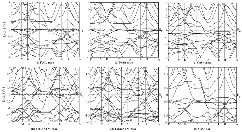
Figure S14: The band structures of (a) FeGe NSOC, (b) FeGe AFM NSOC, (c) FeSn NSOC, (d) FeSn AFM NSOC, (e) CoSn NSOC, and (f) CoSn SOC cases.

V.2 Tight-binding models of FeSn and CoSn

As FeSn and CoSn share similar band structures with FeGe, we build TB models for them using the same model of FeGe in Eq. S2.51 and Eq. S2.54. The fitted TB parameters are slightly different from that of FeGe, as tabulated in Table S20, S21, and the corresponding band structures are shown in Fig. S15. Compared with FeGe, FeSn has very close onsite and hopping parameters, while CoSn has lower onsite energies due to the shifted $E_{f}$, and hoppings being close to FeGe.

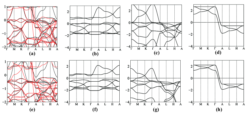
Figure S15: The fitted TB band structures for FeSn (a)-(e) and CoSn (e)-(h). (a). Fitted bands for FeSn of the decoupled model in Eq. S2.55, where red lines are fitted TB bands and black dashed lines are DFT bands. (b)-(d): Band structure of the decoupled $H_{1}(\bm{k})$, $H_{2}(\bm{k})$, and $H_{3}(\bm{k})$ defined in Eq. S2.54, respectively. (e)-(h) are similar figures for CoSn.

Parameter	$\mu_{p_{xy}^{t}}$	$\mu_{d_{1}}$	$\mu_{d_{2}}$	$t_{d_{1}}^{NN}$	$t_{d_{2}}^{NN}$	$t_{d_{2}}^{NNN}$	$t_{d_{1},d_{2}}^{NN}$	$t_{d_{1},d_{2}}^{NNN}$	$t_{p_{xy}^{t},d_{1}}^{NN}$	$t_{p_{xy}^{t},d_{1}}^{NNN}$	$t_{p_{xy}^{t},d_{2}}^{NN}$	$t_{d}^{4N1}$	$t_{d}^{4N2}$	$t_{d}^{4N3}$
Value	-1.37	-0.79	0.11	0.47	0.11	0.05	-0.08	0.15	-0.26	0.10	0.31	-0.13	0.05	0.07
Parameter	$\mu_{p_{z}^{h}}$	$\mu_{d_{3}}$	$\mu_{d_{4}}$	$t_{d_{3},d_{4}}^{NN}$	$t_{d_{3}}^{NN}$	$t_{d_{4}}^{NN}$	$t_{d_{4}}^{zNN}$	$t_{p_{z}^{h},d_{4}}^{NN}$	$t_{p_{z}^{h}}^{NN}$	$t_{p_{z}^{h},d_{2}}^{NN}$	$\mu_{p_{z}^{t}}$	$t_{p_{z}^{t}}^{NN}$	$t_{p_{z}^{t},d_{3}}^{NN}$
Value	-1.41	-0.80	-0.78	-0.15	-0.18	0.20	0.10	0.77	-0.46	0.28	0.60	0.30	0.45
Parameter	$\mu_{d_{5}}$	$t_{d_{5}}^{NN}$	$\mu_{b}$	$t_{b}^{NN}$	$t_{b}^{zNN}$	$t_{b,d_{5}}^{NN}$	$t_{b,d_{5}}^{NNN}$
Value	-0.98	-0.20	-0.6	-0.1	0.9	-1.1	0.04

Table S20: Onsite energies and hoppings used in the decoupled TB model of FeSn, where $d_{1}$ to $d_{5}$ denote $d_{xy},d_{x^{2}-y^{2}},d_{xz},d_{yz},d_{z^{2}}$, respectively, $b$ the bonding state, and $p_{i}^{t}$ ($p_{i}^{h}$) denotes the $p_{i}$ orbitals of the trigonal (honeycomb) Ge. For the simplified $H_{3}(\mathbf{k})$ of $d_{z^{2}}$ only, the parameters are $\mu_{d_{5}}=0.61,t_{d_{5}}^{NN}=-0.21,t_{d_{5}}^{zNN}=0.8$. Parameters not listed in the table have zero values.

Parameter	$\mu_{p_{xy}^{t}}$	$\mu_{d_{1}}$	$\mu_{d_{2}}$	$t_{d_{1}}^{NN}$	$t_{d_{2}}^{NN}$	$t_{d_{2}}^{NNN}$	$t_{d_{1},d_{2}}^{NN}$	$t_{d_{1},d_{2}}^{NNN}$	$t_{p_{xy}^{t},d_{1}}^{NN}$	$t_{p_{xy}^{t},d_{1}}^{NNN}$	$t_{p_{xy}^{t},d_{2}}^{NN}$	$t_{d}^{4N1}$	$t_{d}^{4N2}$	$t_{d}^{4N3}$
Value	-1.35	-1.01	-0.21	0.44	0.13	0.04	-0.10	0.16	-0.25	0.07	0.26	-0.14	0.03	0.06
Parameter	$\mu_{p_{z}^{h}}$	$\mu_{d_{3}}$	$\mu_{d_{4}}$	$t_{d_{3},d_{4}}^{NN}$	$t_{d_{3}}^{NN}$	$t_{d_{4}}^{NN}$	$t_{d_{4}}^{zNN}$	$t_{p_{z}^{h},d_{4}}^{NN}$	$t_{p_{z}^{h}}^{NN}$	$t_{p_{z}^{h},d_{2}}^{NN}$	$\mu_{p_{z}^{t}}$	$t_{p_{z}^{t}}^{NN}$	$t_{p_{z}^{t},d_{3}}^{NN}$
Value	-1.91	-1.18	-1.23	-0.12	-0.16	0.20	0.10	0.83	-0.46	0.28	0.60	0.30	0.45
Parameter	$\mu_{d_{5}}$	$t_{d_{5}}^{NN}$	$\mu_{b}$	$t_{b}^{NN}$	$t_{b}^{zNN}$	$t_{b,d_{5}}^{NN}$	$t_{b,d_{5}}^{NNN}$
Value	-1.30	-0.16	-1.0	-0.1	0.9	-1.1	0.04

Table S21: Onsite energies and hoppings used in the decoupled TB model of CoSn, where $d_{1}$ to $d_{5}$ denote $d_{xy},d_{x^{2}-y^{2}},d_{xz},d_{yz},d_{z^{2}}$, respectively, $b$ the bonding state, and $p_{i}^{t}$ ($p_{i}^{h}$) denotes the $p_{i}$ orbitals of the trigonal (honeycomb) Ge. For the simplified $H_{3}(\mathbf{k})$ of $d_{z^{2}}$ only, the parameters are $\mu_{d_{5}}=0.31,t_{d_{5}}^{NN}=-0.15,t_{d_{5}}^{zNN}=0.8$. Parameters not listed in the table have zero values.

V.3 Interaction parameters of FeSn and CoSn

The interaction parameters are computed for FeSn and CoSn using the $d$-full model, i.e., Wannier functions are constructed from $s,p,d$ orbitals of Fe (Co) and $s,p$ orbitals of Sn for FeSn (CoSn), and exclude only the polarization between $d$ orbitals, as tabulated in Table S23 and S27.

In Table S24 and S28, we list the $O_{h}$-symmetrized onsite Coulomb matrices elements $U_{ij}$ and $J_{ij}$ for FeSn and CoSn, respectively.

In Table S25 and S29, we list the fitted Coulomb elements $U_{ij}$ and $J_{ij}$ using Slater integrals $F_{0},F_{2},F_{4}$ for FeSn and CoSn, while in Table S26 and S30, we list the fitted Coulomb elements using Slater integrals $F_{0}$ and $F_{2}$ only and fix $F_{4}=0.625F_{2}$ for FeSn and CoSn, respectively.

In Table S22, we list the Hubbard-Kanamori parameters for FeGe, FeSn, and CoSn, which share close values. Compared with FeGe, FeSn has onsite intra-orbital Hubbard $\mathcal{U}\approx 4$ eV which is about 0.2 eV smaller than FeGe, while for CoSn, $\mathcal{U},\mathcal{U}^{\prime}$ are both about 0.2 eV smaller than FeGe.

The two quasi-flat bands at $E_{f}$ and large Coulomb interactions in FeGe and FeSn give rise to the AFM order. FeSn also has multiple vHS close to $E_{f}$ in the AFM phase, as shown in Fig. S14(d), but unlike FeGe there is no CDW transition reported, which requires future investigation. For CoSn, despite the similar Coulomb interaction as FeGe and FeSn, there is no AFM or CDW reported, which is possibly due to that the two flat bands in CoSn are fully filled and no vHSs close to $E_{f}$.

Hubbard-Kanamori	$\mathcal{U}$	$\mathcal{U}^{\prime}$	$\mathcal{J}$
FeGe	4.18	2.73	0.72
FeSn	3.99	2.66	0.66
CoSn	3.95	2.54	0.70

Table S22: The Hubbard-Kanamori parameters in the $d$-full model in FeGe, FeSn, and CoSn. These three materials share close interaction parameters, with FeGe being slightly larger. All numbers are in eV.

$U_{ij}$	$z^{2}$	$xz$	$yz$	$x^{2}-y^{2}$	$xy$		$J_{ij}$	$z^{2}$	$xz$	$yz$	$x^{2}-y^{2}$	$xy$
$z^{2}$	3.93	2.79	2.98	2.35	2.37				0.47	0.49	0.86	0.86
$xz$		3.59	2.43	2.46	2.48					0.68	0.68	0.68
$yz$			4.02	2.66	2.67						0.72	0.72
$x^{2}-y^{2}$				4.17	3.40							0.39
$xy$					4.22
$U_{ij}^{NN}$	$z^{2}$	$xz$	$yz$	$x^{2}-y^{2}$	$xy$		$U_{ij}^{NNN}$	$z^{2}$	$xz$	$yz$	$x^{2}-y^{2}$	$xy$
$z^{2}$	1.33	1.32	1.35	1.36	1.36			1.16	1.16	1.16	1.17	1.17
$xz$		1.32	1.33	1.34	1.35				1.17	1.16	1.17	1.17
$yz$			1.37	1.37	1.38					1.16	1.17	1.17
$x^{2}-y^{2}$				1.39	1.40						1.18	1.18
$xy$					1.40							1.18

Table S23: The Coulomb interaction $U_{ij}$ and $J_{ij}$ of $d$ orbitals, and $U_{ij}^{NN}$ and $U_{ij}^{NNN}$ between NN and NNN $d$ in $d-$full model of FeSn. The onsite Hubbard-Kanamori parameters for five $d$ orbitals are $\mathcal{U}=3.99,\mathcal{U}^{\prime}=2.66,\mathcal{J}=0.66$. The averaged NN and NNN interactions are $\overline{U}^{NN}=1.36,\overline{U}^{NNN}=1.17$, with root mean square error being 0.023 and 0.006, respectively. All numbers are in eV.

$U_{ij}$	$z^{2}$	$xz$	$yz$	$x^{2}-y^{2}$	$xy$	$J_{ij}$	$z^{2}$	$xz$	$yz$	$x^{2}-y^{2}$	$xy$
$z^{2}$	4.06	3.00	3.00	2.35	2.33			0.49	0.49	0.86	0.82
$xz$		3.94	2.53	2.55	2.53				0.70	0.71	0.70
$yz$			3.94	2.55	2.53					0.71	0.70
$x^{2}-y^{2}$				4.06	3.23						0.38
$xy$					3.94

Table S24: The Coulomb interaction $U_{ij}$ and $J_{ij}$ of $d$ orbitals for the $d$-full model symmetrized using $O_{h}$ symmetries in FeSn. The root mean square error of the averaged $U_{ij}$ and $J_{ij}$ is 0.177 and 0.069, respectively.

$U_{ij}$	$z^{2}$	$xz$	$yz$	$x^{2}-y^{2}$	$xy$	$J_{ij}$	$z^{2}$	$xz$	$yz$	$x^{2}-y^{2}$	$xy$
$z^{2}$	3.98	2.99	2.99	2.33	2.33			0.49	0.49	0.82	0.82
$xz$		3.98	2.55	2.55	2.55				0.71	0.71	0.71
$yz$			3.98	2.55	2.55					0.71	0.71
$x^{2}-y^{2}$				3.98	3.21						0.38
$xy$					3.98

Table S25: The Coulomb interaction $U_{ij}$ and $J_{ij}$ of $d$ orbitals fitted using Eq. S3.77 in FeSn, where the Slater integrals $F^{0}$, $F^{2}$, and $F_{4}$ are fitted to the full Coulomb matrix $U_{ijkl}$ symmetrized by $O_{h}$ symmetries. The fitted parameters are $F^{0}=2.926,F^{2}=8.092,F^{4}=4.819$. The root mean square error of the fitted $U_{ij}$ and $J_{ij}$ is 0.143 and 0.026, respectively.

$U_{ij}$	$z^{2}$	$xz$	$yz$	$x^{2}-y^{2}$	$xy$	$J_{ij}$	$z^{2}$	$xz$	$yz$	$x^{2}-y^{2}$	$xy$
$z^{2}$	3.99	2.98	2.98	2.34	2.34			0.50	0.50	0.83	0.83
$xz$		3.99	2.55	2.55	2.55				0.72	0.72	0.72
$yz$			3.99	2.55	2.55					0.72	0.72
$x^{2}-y^{2}$				3.99	3.19						0.40
$xy$					3.99

Table S26: The Coulomb interaction $U_{ij}$ and $J_{ij}$ of $d$ orbitals fitted using Eq. S3.77 in FeSn, where the Slater integrals $F^{0}$, $F^{2}$ are fitted to the full Coulomb matrix $U_{ijkl}$ symmetrized by $O_{h}$ symmetries, while $F^{4}=0.625F^{2}$ are fixed. The fitted parameters are $F^{0}=2.926,F^{2}=8.024,F^{4}=5.015$. The root mean square error of the fitted $U_{ij}$ and $J_{ij}$ is 0.144 and 0.029, respectively.

$U_{ij}$	$z^{2}$	$xz$	$yz$	$x^{2}-y^{2}$	$xy$		$J_{ij}$	$z^{2}$	$xz$	$yz$	$x^{2}-y^{2}$	$xy$
$z^{2}$	3.94	2.77	2.88	2.21	2.22				0.51	0.53	0.89	0.90
$xz$		3.65	2.36	2.39	2.40					0.73	0.73	0.73
$yz$			3.97	2.48	2.49						0.76	0.77
$x^{2}-y^{2}$				4.07	3.25							0.42
$xy$					4.11
$U_{ij}^{NN}$	$z^{2}$	$xz$	$yz$	$x^{2}-y^{2}$	$xy$		$U_{ij}^{NNN}$	$z^{2}$	$xz$	$yz$	$x^{2}-y^{2}$	$xy$
$z^{2}$	1.32	1.32	1.33	1.36	1.36			1.17	1.16	1.17	1.17	1.18
$xz$		1.33	1.33	1.36	1.37				1.17	1.17	1.18	1.18
$yz$			1.35	1.37	1.38					1.17	1.17	1.18
$x^{2}-y^{2}$				1.41	1.42						1.19	1.19
$xy$					1.42							1.19

Table S27: The Coulomb interaction $U_{ij}$ and $J_{ij}$ of $d$ orbitals, and $U_{ij}^{NN}$ and $U_{ij}^{NNN}$ between NN and NNN $d$ in $d-$full model of CoSn. The onsite Hubbard-Kanamori parameters for five $d$ orbitals are $\mathcal{U}=3.95,\mathcal{U}^{\prime}=2.54,\mathcal{J}=0.70$. The averaged NN and NNN interactions are $\overline{U}^{NN}=1.36,\overline{U}^{NNN}=1.17$, with root mean square error being 0.029 and 0.009, respectively. All numbers are in eV.

$U_{ij}$	$z^{2}$	$xz$	$yz$	$x^{2}-y^{2}$	$xy$	$J_{ij}$	$z^{2}$	$xz$	$yz$	$x^{2}-y^{2}$	$xy$
$z^{2}$	4.06	3.00	3.00	2.35	2.33			0.49	0.49	0.86	0.82
$xz$		3.94	2.53	2.55	2.53				0.70	0.71	0.70
$yz$			3.94	2.55	2.53					0.71	0.70
$x^{2}-y^{2}$				4.06	3.23						0.38
$xy$					3.94

Table S28: The Coulomb interaction $U_{ij}$ and $J_{ij}$ of $d$ orbitals for the $d$-full model symmetrized using $O_{h}$ symmetries in CoSn. The root mean square error of the averaged $U_{ij}$ and $J_{ij}$ is 0.216 and 0.035, respectively.

$U_{ij}$	$z^{2}$	$xz$	$yz$	$x^{2}-y^{2}$	$xy$	$J_{ij}$	$z^{2}$	$xz$	$yz$	$x^{2}-y^{2}$	$xy$
$z^{2}$	3.94	2.89	2.89	2.20	2.20			0.53	0.53	0.87	0.87
$xz$		3.94	2.43	2.43	2.43				0.76	0.76	0.76
$yz$			3.94	2.43	2.43					0.76	0.76
$x^{2}-y^{2}$				3.94	3.12						0.41
$xy$					3.94

Table S29: The Coulomb interaction $U_{ij}$ and $J_{ij}$ of $d$ orbitals fitted using Eq. S3.77 in CoSn, where the Slater integrals $F^{0}$, $F^{2}$, and $F_{4}$ are fitted to the full Coulomb matrix $U_{ijkl}$ symmetrized by $O_{h}$ symmetries. The fitted parameters are $F^{0}=2.825,F^{2}=8.522,F^{4}=5.163$. The root mean square error of the fitted $U_{ij}$ and $J_{ij}$ is 0.094 and 0.022, respectively.

$U_{ij}$	$z^{2}$	$xz$	$yz$	$x^{2}-y^{2}$	$xy$	$J_{ij}$	$z^{2}$	$xz$	$yz$	$x^{2}-y^{2}$	$xy$
$z^{2}$	3.95	2.88	2.88	2.21	2.21			0.53	0.53	0.87	0.87
$xz$		3.95	2.43	2.43	2.43				0.76	0.76	0.76
$yz$			3.95	2.43	2.43					0.76	0.76
$x^{2}-y^{2}$				3.95	3.11						0.42
$xy$					3.95

Table S30: The Coulomb interaction $U_{ij}$ and $J_{ij}$ of $d$ orbitals fitted using Eq. S3.77 in CoSn, where the Slater integrals $F^{0}$, $F^{2}$ are fitted to the full Coulomb matrix $U_{ijkl}$ symmetrized by $O_{h}$ symmetries, while $F^{4}=0.625F^{2}$ are fixed. The fitted parameters are $F^{0}=2.825,F^{2}=8.475,F^{4}=5.297$. The root mean square error of the fitted $U_{ij}$ and $J_{ij}$ is 0.095 and 0.023, respectively.

Appendix VI Building models for 1:6:6 class from 1:1 class: Application to MgFe6Ge6

In previous sections, we studied in detail the electronic properties of FeGe, FeSn, and CoSn in detail. These materials belong to the 1:1 class in SG 191, and form the fundamental building blocks for the 1:6:6 material family Venturini (2006); Fredrickson et al. (2008) with chemical formula MT₆Z₆, where M is a metallic element (including Mg, Sc, and rare-earth elements, etc), T a transition metal, and Z a main group element (including Si, Ga, Ge, and Sn). The 1:6:6 family materials can be seen as the doubled 1:1 materials along the $c$-axis and inserting $M$ atoms in the middle. Usually, the electrons of M atoms are away from the Fermi level, which means it is possible to construct bands of 1:6:6 materials from 1:1 materials by doubling the unit cell and treating the orbitals of M as perturbations. We test this strategy by focusing on one representative 1:6:6 material MgFe₆Ge₆ and build its band structure from FeGe in this section. This strategy is expected to work for the other 1:6:6 materials, and the minimal TB model we build for FeSn and CoSn could also be used to construct their corresponding 1:6:6 materials.

VI.1 Crystal structure and band structure of MgFe6Ge6

Similar to FeGe, $\text{MgFe}_{6}\text{Ge}_{6}$ has SG 191 $P6/mmm$ symmetry in the paramagnetic phase. The lattice constants are $a=5.071\AA$ and $c=8.046\AA$Mazet et al. (2013). The crystal structure is shown in Fig. S16(a), where

• Mg atoms form a trigonal lattice on $z=0.5$ plane in the unit cell, i.e., $1b$ Wyckoff position.

• Fe atoms form two kagome layers on $z=0.252$ and $z=0.748$ planes, i.e., $6i$ Wyckoff position.

• Two Ge atoms form two trigonal lattices on $z=0.159$ and $z=0.841$ planes, i.e., $2e$ Wyckoff position, which differs from FeGe where the trigonal Ge atoms lie on the same plane with Fe.

• Four Ge atoms form two honeycomb lattices on $z=0$ and $z=0.5$ planes, i.e., $2c$ and $2d$ Wyckoff positions.

The coordinates of these Wyckoff positions can be found in Table S2. We emphasize that $\text{MgFe}_{6}\text{Ge}_{6}$ can be viewed as a twofold supercell of FeGe by adding Mg atoms in the middle and (slightly) shifting the Ge atoms on trigonal lattice away (about 0.7 Å) from the kagome layer formed by Fe atoms. Indeed we find the band structure of $\text{MgFe}_{6}\text{Ge}_{6}$ is similar and related to the band structure of FeGe.

The band structure of $\text{MgFe}_{6}\text{Ge}_{6}$ in the PM phase without SOC is shown in Fig. S16(b). As $\text{MgFe}_{6}\text{Ge}_{6}$ can be seen as a perturbed twofold supercell of FeGe, we unfold the band structure of $\text{MgFe}_{6}\text{Ge}_{6}$ to the BZ of FeGe in Fig. S16(c) using VaspBandUnfolding packageZheng (2018); Popescu and Zunger (2012). The unfolded band structure is very close to the band structure of FeGe. In Fig. S16(d)-(f), we show the projections of $d$ orbitals of Fe in $\text{MgFe}_{6}\text{Ge}_{6}$. The orbital weights of Fe $d$ orbitals in $\text{MgFe}_{6}\text{Ge}_{6}$ are also very close to FeGe. The $p$ orbitals of Ge atoms also have similar distributions as in FeGe and are not shown for simplicity. The orbitals of Mg atoms are far away from the Fermi level, with the $s$ orbital being about 3 eV above $E_{f}$.

In Table S31, we show the filling of each orbital in MgFe6Ge6 in the PM phae. Compared with the filling of FeGe in Table S4, MgFe6Ge6 has one more valence given by the $s$ orbital of Mg per FeGe layer (2 extra electrons in total). The extra valence is mainly contributed by Ge and Mg, while the filling of Fe is almost unchanged. This is also verified by the $d$ orbital projections of Fe which are very close for FeGe and MgFe6Ge6. In Fig. S17, we compare the total DOS of FeGe and MgFe6Ge6, which show a good match at the Fermi level. The extra valence electrons in MgFe6Ge6 mainly change the DOS below -0.5 eV.

The above observations inspire us to understand the band structure of $\text{MgFe}_{6}\text{Ge}_{6}$ via the band structure of FeGe. In the next section, we will show the procedure of constructing the TB models for $\text{MgFe}_{6}\text{Ge}_{6}$ based on the TB model of FeGe. In short, we start from the TB models of the FeGe but with an enlarged unit cell, such that two layers of FeGe have been included. Then we treat Mg atoms as a perturbation. We remark that the inserted 1 atom in the 1:6:6 family usually provides extra valence electrons and changes the Fermi level. This should be treated carefully when constructing the TB model for 1:6:6 using 1:1 building blocks. However, for MgFe6Ge6, the fillings of $d$ orbitals have little change, and we use the same Fermi level in the minimal TB model for simplicity.

Before constructing the TB models, we also mention that $\text{MgFe}_{6}\text{Ge}_{6}$ develops an AFM order at $T_{N}=501K$ with the magnetic moment on Fe atoms being $m=1.59$ $\mu_{B}$ at $2K$ along the $\bm{c}$-axisMazet et al. (2013). The crystal structure, band structure, and $d$ orbital projections in the AFM phase are shown in Fig. S18. The computed magnetic moment on Fe is $1.79$ $\mu_{B}$ in DFT. We point out that the magnetic structure of $\text{MgFe}_{6}\text{Ge}_{6}$ is almost identical to the magnetic structure of FeGe. Note that in the PM phase the unit cell of $\text{MgFe}_{6}\text{Ge}_{6}$ is a doubled FeGe with extra Mg atoms, while in the AFM phase of FeGe, the magnetic unit cell is the same for $\text{MgFe}_{6}\text{Ge}_{6}$ and FeGe. This further confirms the similarity and connection between $\text{MgFe}_{6}\text{Ge}_{6}$ and FeGe. We also remark that $\text{MgFe}_{6}\text{Ge}_{6}$ only appear as powder in literatureMazet et al. (2013).

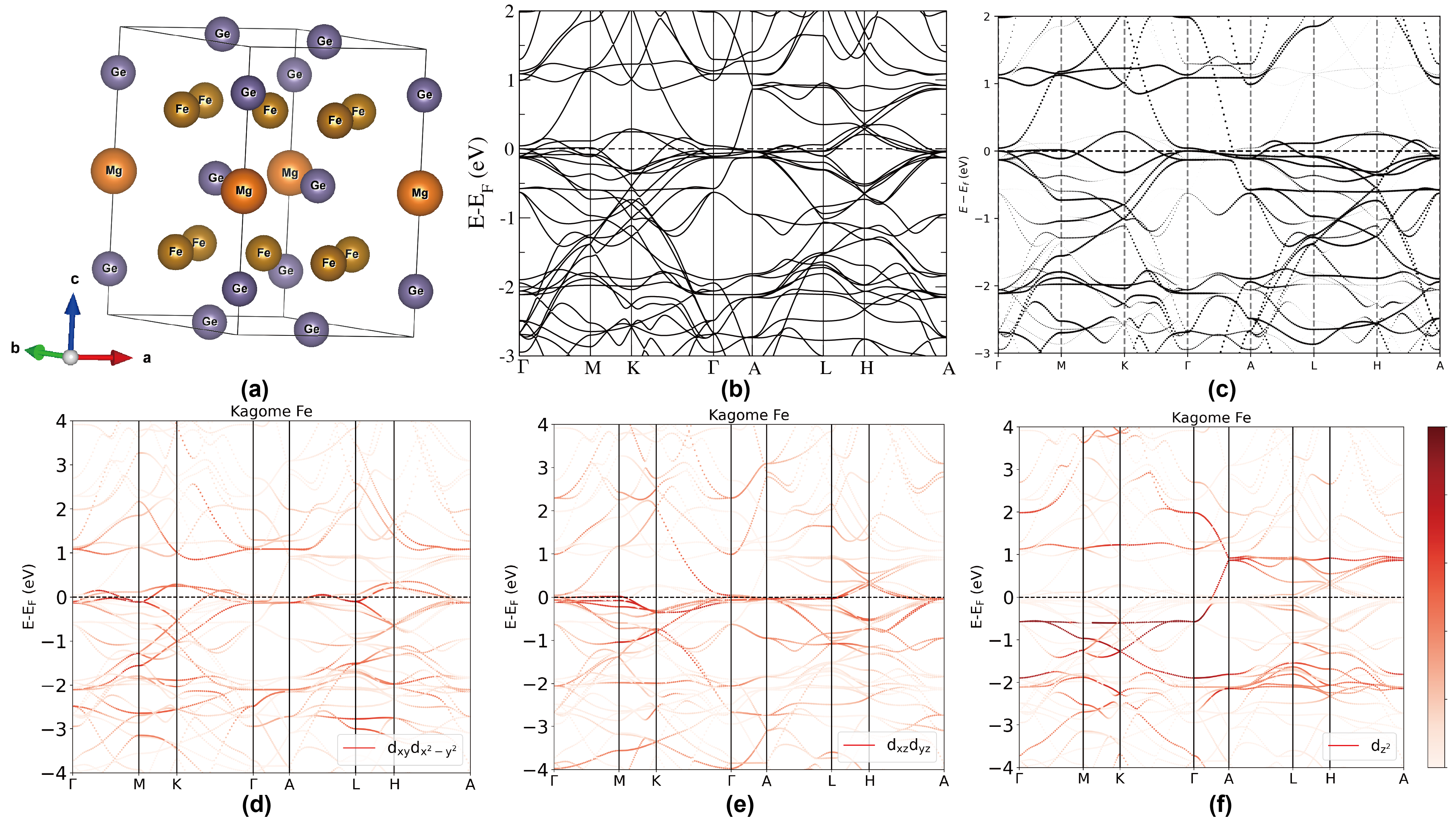
Figure S16: (a) Crystal structure and (b) band structure without SOC of $\text{MgFe}_{6}\text{Ge}_{6}$ in the paramagnetic phase. (c) Unfolded band structure of $\text{MgFe}_{6}\text{Ge}_{6}$. (d)-(f) are orbital projections of the bands in the PM phase of $\text{MgFe}_{6}\text{Ge}_{6}$, where (d) is the projection of $d_{xy},d_{x^{2}-y^{2}}$, (e) $d_{xz},d_{yz}$, and (f) $d_{z^{2}}$ orbitals of Fe. The band structure and orbital weights of $\text{MgFe}_{6}\text{Ge}_{6}$ are very close to FeGe after folding the BZ in the $k_{3}$ direction.

	Orbitals	$s$	$p_{z}$	$p_{x}$	$p_{y}$	$d_{z^{2}}$	$d_{xz}$	$d_{yz}$	$d_{x^{2}-y^{2}}$	$d_{xy}$	Total
PM filling	Fe	0.61	0.28	0.31	0.27	1.44	1.64	1.50	1.32	1.49	8.86
	Tri-Ge	1.46	0.70	0.63	0.62	-	-	-	-	-	3.40
	Hon-Ge	1.49	0.72	0.62	0.64	-	-	-	-	-	3.46
	Mg	0.4	-	-	-	-	-	-	-	-	0.4
PM DOS@$E_{f}$	Fe	-	-	-	-	0.05	0.27	0.26	0.30	0.05	0.94

Table S31: The filling and density of states (DOS) of MgFe6Ge6 in the PM phase, calculated from a Wannier TB built from Mg $s$, Fe $s,p,d$, and Ge $s,p$ orbitals. The total filling is 74.2, which is close to the number of valence electrons, i.e., 74 (given by $4s^{1}3d^{7}$ of 3 Fe,$4s^{2}4p^{2}$ of 3 Ge, and $3s^{2}$ of Mg).

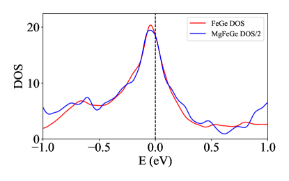
Figure S17: Comparison of DOS in PM phase between FeGe and MgFe6Ge6, where the DOS of MgFe6Ge6 has divided by 2 in order to compare with FeGe. The two DOS curves show good agreements at the Fermi level where the large peak is given by the flat band.

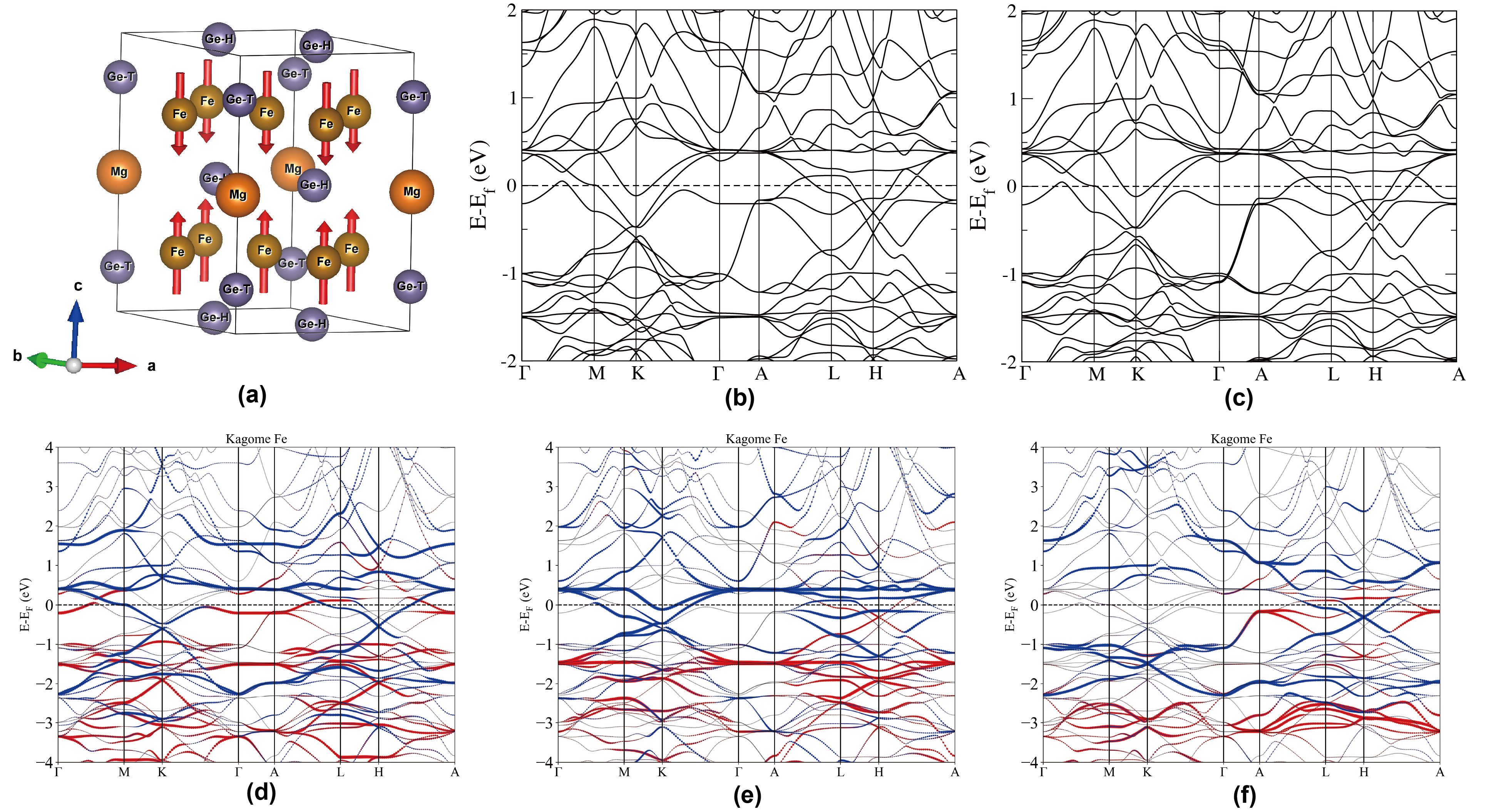
Figure S18: (a) Crystal structure, band structure (b) without SOC, and (c) with SOC of $\text{MgFe}_{6}\text{Ge}_{6}$ in the AFM phase. (d)-(f) are orbital projections of the bands in the AFM phase of $\text{MgFe}_{6}\text{Ge}_{6}$, where (d) is the projection of $d_{xy},d_{x^{2}-y^{2}}$, (e) $d_{xz},d_{yz}$, and (f) $d_{z^{2}}$ orbitals of Fe, where blue and red colors denote $d$ orbitals of opposite spins of Fe on the same kagome plane. The band structure and orbital weights of $\text{MgFe}_{6}\text{Ge}_{6}$ are very close to FeGe in the AFM phase. The calculated magnetic moment in $\text{MgFe}_{6}\text{Ge}_{6}$ is 1.79 $\mu_{B}$ per Fe atom which is larger than that in FeGe which is 1.53 $\mu_{B}$.

VI.2 Tight-binding models

TB models of $\text{MgFe}_{6}\text{Ge}_{6}$, denoted by $H^{[166]}(\bm{k})$, can be constructed using the TB models of FeGe defined in Eq. S2.51 and Eq. S2.54, denoted as $H^{[11]}(\bm{k})$.

We first consider the TB model of a perfect twofold supercell (SC) of FeGe with two identical unit cells in the $z$-direction, in which the basis $\bm{a}_{3}$ is doubled while $\bm{b}_{3}$ of BZ is halved. The TB model $H^{[\text{SC}]}(\bm{k})$ is

$$H^{[\text{SC}]}(\bm{k})=H^{[11]}(k_{1},k_{2},\frac{k_{3}}{2})\oplus H^{[11]}(k_{1},k_{2},\frac{k_{3}}{2}+\pi),$$ (S6.83)

where the bands on $k_{3}=0,\pi$ ($k_{3}=\pm\frac{\pi}{2}$) planes of $H^{[11]}(\bm{k})$ are folded onto the $k_{3}=0$ ($k_{3}=\pi$) plane of $H^{[\text{SC}]}$. In this case, the bands on the $k_{3}=\pi$ plane are always twofold degenerate, as a result of perfect SC.

More rigorously, we consider the effect of the inclusion of Mg atoms and the dislocation of trigonal Ge atoms in the TB model for $\text{MgFe}_{6}\text{Ge}_{6}$, which breaks the perfect twofold SC. The inclusion of Mg atoms has larger effects on the band structure. We use $d_{i}^{1}$ and $d_{i}^{2}$ to denote the $d_{i}$ orbitals on the kagome layer of $z=0.252$ and $z=0.748$ plane, $p_{i}^{h_{1}}$ and $p_{i}^{h_{2}}$ to denote the $p_{i}$ orbitals on the honeycomb layer of $z=0$ and $z=\frac{1}{2}$ plane, and $p_{i}^{t_{1}}$ and $p_{i}^{t_{2}}$ to denote the $p_{i}$ orbitals on the trigonal layer of $z=0.159$ and $z=0.841$ plane, respectively. Following the method used in FeGe, we split the orbitals into three groups and construct TB models for them separately. As the onsite energy of the Mg $s$ orbital is much higher than other orbitals (onsite difference of about 4 eV) in the model, the coupling with the $s$ orbital of the Mg atom will be treated as a perturbation which will modify the hoppings between certain orbitals (see Section VI.2.4).

VI.2.1 $H_{1}(k)$

The first group of orbitals contains $p_{x},p_{y}$ orbitals of Ge at $2e$ (denoted by $p_{xy}^{t}$), $d_{xy},d_{x^{2}-y^{2}}$ (denoted by $d_{1},d_{2}$) orbitals of Fe at $6i$. We also add $p_{z}$ orbitals of honeycomb Ge at $2c$ and $2d$ (denoted by $p_{z}^{h_{i}}$) here to introduce the $S$-matrix, where in FeGe they are considered later in the final model in Eq. S2.51. The TB model has the form

$$H_{1}^{[166]}(\bm{k})= \left(\begin{array}[]{ccc|ccc|cc}H_{p_{xy}^{t}}(k_{1},k_{2})&S_{p_{xy}^{t_{1}},d_{1}^{1}}(\bm{k})&S_{p_{xy}^{t_{1}},d_{2}^{1}}(\bm{k})&\bm{0}&\bm{0}&\bm{0}&\bm{0}&\bm{0}\\ &H_{d_{1}}(k_{1},k_{2})&S_{d_{1},d_{2}}(k_{1},k_{2})&\bm{0}&\bm{0}&\bm{0}&\bm{0}&\bm{0}\\ &&H_{d_{2}}(k_{1},k_{2})&\bm{0}&\bm{0}&\bm{0}&S_{p_{z}^{h_{1}},d_{2}^{1}}^{\dagger}(\bm{k})&S_{p_{z}^{h_{2}},d_{2}^{1}}^{\dagger}(\bm{k})\\ \hline\cr&&&H_{p_{xy}^{t}}(k_{1},k_{2})&S_{p_{xy}^{t_{2}},d_{1}^{2}}(\bm{k})&S_{p_{xy}^{t_{2}},d_{2}^{2}}(\bm{k})&\bm{0}&\bm{0}\\ &&&&H_{d_{1}}(k_{1},k_{2})&S_{d_{1},d_{2}}(k_{1},k_{2})&\bm{0}&\bm{0}\\ &&&&&H_{d_{2}}(k_{1},k_{2})&S_{p_{z}^{h_{1}},d_{2}^{2}}^{\dagger}(\bm{k})&S_{p_{z}^{h_{2}},d_{2}^{2}}^{\dagger}(\bm{k})\\ \hline\cr&&&&&&H_{p_{z}^{h_{1}}}(\bm{k})&\\ h.c.&&&&&&&H_{p_{z}^{h_{2}}}(\bm{k})\\ \end{array}\right)$$ (S6.84)

The coupling terms between $p_{xy}^{t}$ and $d_{1,2}$ orbitals are

$$S_{p_{xy}^{t_{1}},d_{1}^{1}}(\bm{k}) =e^{i\Delta_{KT}k_{3}}S_{p_{xy}^{t},d_{1}}^{\text{inplane}}(k_{1},k_{2}),$$ (S6.85)

$$S_{p_{xy}^{t_{1}},d_{2}^{1}}(\bm{k}) =e^{i\Delta_{KT}k_{3}}S_{p_{xy}^{t},d_{2}}^{\text{inplane}}(k_{1},k_{2}),$$

$$S_{p_{xy}^{t_{2}},d_{1}^{2}}(\bm{k}) =e^{-i\Delta_{KT}k_{3}}S_{p_{xy}^{t},d_{1}}^{\text{inplane}}(k_{1},k_{2}),$$

$$S_{p_{xy}^{t_{2}},d_{2}^{2}}(\bm{k}) =e^{-i\Delta_{KT}k_{3}}S_{p_{xy}^{t},d_{2}}^{\text{inplane}}(k_{1},k_{2}),$$

where $\Delta_{KT}=0.09$ is the dislocation of Ge atoms in the $z$-direction, and $S_{p_{xy}^{t},d_{i}}^{\text{inplane}}(k_{1},k_{2})$ is the same as $S_{p_{xy}^{t},d_{i}}(\bm{k})$ defined in Eq. S2.23. The coupling terms between $p_{z}^{h}$ and $d_{2}$ orbitals are:

$$S_{p_{z}^{h_{1}},d_{2}^{1}}(\bm{k}) =t_{p_{z}^{h^{1}},d_{2}}^{NN}e^{i\frac{k_{3}}{4}}S_{p_{z}^{h},d_{2}}^{\text{inplane}}(k_{1},k_{2}),$$ (S6.86)

$$S_{p_{z}^{h_{1}},d_{2}^{2}}(\bm{k}) =-t_{p_{z}^{h^{1}},d_{2}}^{NN}e^{-i\frac{k_{3}}{4}}S_{p_{z}^{h},d_{2}}^{\text{inplane}}(k_{1},k_{2}),$$

$$S_{p_{z}^{h_{2}},d_{2}^{1}}(\bm{k}) =-t_{p_{z}^{h_{2}},d_{2}}^{NN}e^{-i\frac{k_{3}}{4}}S_{p_{z}^{h},d_{2}}^{\text{inplane}}(k_{1},k_{2}),$$

$$S_{p_{z}^{h_{2}},d_{2}^{2}}(\bm{k}) =t_{p_{z}^{h^{2}},d_{2}}^{NN}e^{i\frac{k_{3}}{4}}S_{p_{z}^{h},d_{2}}^{\text{inplane}}(k_{1},k_{2}),$$

$$S_{p_{z}^{h},d_{2}}^{\text{inplane}}(k_{1},k_{2}) =\left(\begin{matrix}e^{\frac{i}{6}(k_{1}+2k_{2})}&e^{\frac{i}{6}(k_{1}-k_{2})}&e^{-\frac{i}{6}(2k_{1}+k_{2})}\\ e^{-\frac{i}{6}(k_{1}+2k_{2})}&e^{-\frac{i}{6}(k_{1}-k_{2})}&e^{\frac{i}{6}(2k_{1}+k_{2})}\\ \end{matrix}\right),$$

where $t_{p_{z}^{h^{1}},d_{4}}^{NN}$ and $t_{p_{z}^{h^{2}},d_{4}}^{NN}$ can take independent values. $H_{p_{z}^{h_{1}}}(k_{1},k_{2}),H_{p_{z}^{h_{2}}}(k_{1},k_{2})$ have the same form as $H_{p_{z}^{h}}(k_{1},k_{2})$ in LABEL:Eq_ham2_matrix_blocks, but $\mu_{p_{z}^{h_{i}}},t_{p_{z}^{h_{i}}}^{NN}$ can be different. This is because the honeycomb Ge’s in MgFe₆Ge₆ form two honeycomb lattices on $z=0$ and $z=0.5$ planes which are symmetry-independent. Notice that in FeGe the honeycomb layers are related by lattice translations, but in MgFe₆Ge₆ there is no symmetry that relates them. In fact, the Mg atoms lie on the honeycomb layer on $z=\frac{1}{2}$ plane which indeed makes them inequivalent. Other matrix blocks have the same form as in Eq. S2.23.

VI.2.2 $H_{2}(k)$

The second group has $p_{z}$ orbitals of Ge at $2c$ and $2d$ (denoted by $p_{z}^{h_{1}}$ and $p_{z}^{h_{2}}$), $p_{z}$ orbitals of Ge at $2e$ (denoted by $p_{z}^{t}$), and $d_{xz},d_{yz}$ (denoted by $d_{3},d_{4}$) orbitals of Fe at $6i$. The TB Hamiltonian has the form

$$H_{2}^{[166]}(\bm{k})= \left(\begin{array}[]{cc|cc|cc|cc}H_{p_{z}^{h_{1}}}(k_{1,2})&\bm{0}&0&0&\bm{0}&S_{p_{z}^{h_{1}},d_{4}^{1}}(\bm{k})&\bm{0}&S_{p_{z}^{h_{1}},d_{4}^{2}}(\bm{k})\\ &H_{p_{z}^{h_{2}}}(k_{1,2})&0&0&\bm{0}&S_{p_{z}^{h_{2}},d_{4}^{1}}(\bm{k})&\bm{0}&S_{p_{z}^{h_{2}},d_{4}^{2}}(\bm{k})\\ \hline\cr&&\epsilon_{p_{z}^{t}}&S_{p_{z}^{t}}^{z}(k_{3})&S_{p_{z}^{t_{1}},d_{3}^{1}}(\bm{k})&\bm{0}&\bm{0}&\bm{0}\\ &&&\epsilon_{p_{z}^{t}}&\bm{0}&\bm{0}&S_{p_{z}^{t_{2}},d_{3}^{2}}(\bm{k})&\bm{0}\\ \hline\cr&&&&H_{d_{3}}(k_{1,2})&S_{d_{3},d_{4}}(k_{1,2})&S_{d_{3}^{1},d_{3}^{2}}(\bm{k})&\bm{0}\\ &&&&&H_{d_{4}}(k_{1,2})&\bm{0}&S_{d_{4}^{1},d_{4}^{2}}(\bm{k})\\ \hline\cr&&&&&&H_{d_{3}}(k_{1,2})&S_{d_{3},d_{4}}(k_{1,2})\\ h.c.&&&&&&&H_{d_{4}}(k_{1,2})\\ \end{array}\right),$$ (S6.87)

where we use $k_{1,2}=(k_{1},k_{2})$, and $H_{p_{z}^{h_{i}}}(k_{1,2})$ have the same form as $H_{p_{z}^{h}}(k_{1},k_{2})$ in LABEL:Eq_ham2_matrix_blocks, but hopping parameters can be different. The $d_{i=3,4}$ Hamiltonians are

$$H_{d_{i}}(k_{1},k_{2}) =\mu_{d_{i}}\bm{1}_{3}+t_{d_{i}}^{NN}H_{\text{kagome}}^{\text{inplane},xz}(k_{1},k_{2}),$$ (S6.88)

$$S_{d_{i}^{1},d_{i}^{2}}(\bm{k}) =\left(t_{d_{i}}^{zNN,+}e^{i\frac{k_{3}}{2}}+t_{d_{i}}^{zNN,-}e^{-i\frac{k_{3}}{2}}\right)\bm{1}_{3}$$

$$H_{\text{kagome}}^{\text{inplane},xz}(k_{1},k_{2}) =\left(\begin{matrix}0&\cos(\frac{k_{2}}{2})&-\cos(\frac{k_{1}+k_{2}}{2})\\ &0&\cos(\frac{k_{1}}{2})\\ h.c.&&0\\ \end{matrix}\right),$$

Notice that we set the $z$-directional distance between two $d$ orbitals to be $\Delta_{KK}=\frac{1}{2}$ for simplicity (i.e., $e^{\pm i\frac{k_{3}}{2}}$ term in Eq. S6.88), whose accurate value is 0.496.

The coupling terms between $p_{z}^{h}$ and $d_{4}$ orbitals are:

$$S_{p_{z}^{h_{1}},d_{4}^{1}}(\bm{k}) =t_{p_{z}^{h^{1}},d_{4}}^{NN}e^{i\frac{k_{3}}{4}}S_{p_{z}^{h},d_{4}}^{\text{inplane}}(k_{1},k_{2}),$$ (S6.89)

$$S_{p_{z}^{h_{1}},d_{4}^{2}}(\bm{k}) =t_{p_{z}^{h^{1}},d_{4}}^{NN}e^{-i\frac{k_{3}}{4}}S_{p_{z}^{h},d_{4}}^{\text{inplane}}(k_{1},k_{2}),$$

$$S_{p_{z}^{h_{2}},d_{4}^{1}}(\bm{k}) =t_{p_{z}^{h_{2}},d_{4}}^{NN}e^{-i\frac{k_{3}}{4}}S_{p_{z}^{h},d_{4}}^{\text{inplane}}(k_{1},k_{2}),$$

$$S_{p_{z}^{h_{2}},d_{4}^{2}}(\bm{k}) =t_{p_{z}^{h_{2}},d_{4}}^{NN}e^{i\frac{k_{3}}{4}}S_{p_{z}^{h},d_{4}}^{\text{inplane}}(k_{1},k_{2}),$$

$$S_{p_{z}^{h},d_{4}}^{\text{inplane}}(k_{1},k_{2}) =\left(\begin{matrix}-e^{\frac{i}{6}(k_{1}+2k_{2})}&e^{\frac{i}{6}(k_{1}-k_{2})}&-e^{-\frac{i}{6}(2k_{1}+k_{2})}\\ e^{-\frac{i}{6}(k_{1}+2k_{2})}&-e^{-\frac{i}{6}(k_{1}-k_{2})}&e^{\frac{i}{6}(2k_{1}+k_{2})},\\ \end{matrix}\right),$$

where $t_{p_{z}^{h^{1}},d_{4}}^{NN}$ and $t_{p_{z}^{h^{2}},d_{4}}^{NN}$ can take independent values, as honeycomb Ge’s on $z=0$ and $z=0.5$ planes are symmetry-independent. The coupling terms between $p_{z}^{t}$ and $p_{z}^{t}$, as well as $p_{z}^{t}$ and $d$ orbitals, are

$$S_{p_{z}^{t}}^{z}(k_{3}) =t_{p_{z}^{t}}^{NN}e^{-i\Delta_{TT}k_{3}},$$ (S6.90)

$$S_{p_{z}^{t_{1}},d_{3}^{1}}(\bm{k}) =e^{i\Delta_{KT}k_{3}}\cdot t_{p_{z}^{t},d_{3}}^{NN}\cdot 2i\left(\begin{matrix}\sin(\frac{k_{1}}{2})&\sin(\frac{k_{1}+k_{2}}{2})&\sin(\frac{k_{2}}{2})\\ \end{matrix}\right),$$

$$S_{p_{z}^{t_{2}},d_{3}^{2}}(\bm{k}) =e^{-i\Delta_{KT}k_{3}}\cdot t_{p_{z}^{t},d_{3}}^{NN}\cdot 2i\left(\begin{matrix}\sin(\frac{k_{1}}{2})&\sin(\frac{k_{1}+k_{2}}{2})&\sin(\frac{k_{2}}{2})\\ \end{matrix}\right),$$

where $\Delta_{TT}=0.32$ is the distance in the $z$-direction between two closest trigonal Ge atoms, and $\Delta_{KT}=0.09$ is the dislocation of trigonal Ge atoms in the $z$-direction from the kagome layer. Other matrix blocks are the same as in LABEL:Eq_ham2_matrix_blocks. Notice that as in FeGe, the hopping between $d_{4}$ and $p_{z}^{t}$ is forbidden by the $M_{120}(=M_{y})$ symmetry.

VI.2.3 $H_{3}(k)$

For the third group of orbitals, i.e., $d_{z^{2}}$ of Fe at $6i$ and the bonding states of honeycomb Ge at $b^{1}@3f$ and $b^{2}@3g$ ($3f$ and $3g$ are on $z=0,\frac{1}{2}$ planes, respectively, as shown in Table S2), the TB Hamiltonian has the form

$$H_{3}^{[166]}(\bm{k}) =\left(\begin{array}[]{cc|cc}H_{b^{1}}(k_{1},k_{2})&S_{b^{1},b^{2}}(k_{3})&S_{b^{1},d_{5}^{1}}(\bm{k})&S_{b^{1},d_{5}^{2}}(\bm{k})\\ &H_{b^{2}}(k_{1},k_{2})&S_{b^{2},d_{5}^{1}}(\bm{k})&S_{b^{2},d_{5}^{2}}(\bm{k})\\ \hline\cr&&H_{d_{5}}(k_{1},k_{2})&S_{d_{5}^{1},d_{5}^{2}}(k_{3})\\ h.c.&&&H_{d_{5}}(k_{1},k_{2})\\ \end{array}\right),$$ (S6.91)

$$S_{d_{5}^{1},d_{5}^{2}}(k_{3}) =(t_{d_{5}}^{zNN,+}e^{i\frac{k_{3}}{2}}+t_{d_{5}}^{zNN,-}e^{-i\frac{k_{3}}{2}})\mathbf{1}_{3}$$

$$S_{b^{1},b^{2}}(k_{3}) =(t_{b}^{zNN,+}e^{i\frac{k_{3}}{2}}+t_{b}^{zNN,-}e^{-i\frac{k_{3}}{2}})\mathbf{1}_{3}$$

$$S_{b^{1},d_{5}^{1}}(\bm{k}) =e^{i\frac{k_{3}}{4}}(t_{b^{1},d_{5}}^{NN}+t_{b^{1},d_{5}}^{NNN}H_{\text{kagome}}^{\text{inplane},z^{2}}(k_{1},k_{2}))$$

$$S_{b^{1},d_{5}^{2}}(\bm{k}) =S_{b^{1},d_{5}^{1}}(k_{1},k_{2},-k_{3})$$

$$S_{b^{2},d_{5}^{1}}(\bm{k}) =e^{-i\frac{k_{3}}{4}}(t_{b^{2},d_{5}}^{NN}+t_{b^{2},d_{5}}^{NNN}H_{\text{kagome}}^{\text{inplane},z^{2}}(k_{1},k_{2}))$$

$$S_{b^{2},d_{5}^{2}}(\bm{k}) =S_{b^{2},d_{5}^{1}}(k_{1},k_{2},-k_{3})$$

where $H_{b^{i=1,2}}(\bm{k}),H_{d_{5}}(\bm{k}),H_{\text{kagome}}^{\text{inplane},z^{2}}(\bm{k})$ are defined as in Eq. S2.49. Note that the two sets of bonding states are symmetry-independent as they are on two different Wyckoff positions $3f$ and $3g$ on $z=0,\frac{1}{2}$ planes, respectively, and thus their onsite energies and hopping parameters can take independent values. This is similar to the honeycomb Ge $p_{z}^{h_{1}}@2c,p_{z}^{h_{1}}@2d$, which are symmetry-independent due to the extra Mg atom on $z=\frac{1}{2}$ layer.

Remember that in FeGe, the bonding states are used to introduce $d_{z^{2}}$ weights below $-2$ eV, which are far from $E_{f}$ and less relevant for the low energy physics near $E_{f}$. We build a simpler model of $d_{z^{2}}$ only that captures the band structure close to $E_{f}$. Similarly, for MgFe₆Ge₆, we build $H_{3}(\bm{k})$ using $d_{z^{2}}$ only and refit parameters to the bands near $E_{f}$:

$$H_{3}^{[166]}(\bm{k}) =\left(\begin{array}[]{cc}H_{d_{5}}(k_{1},k_{2})&S_{d_{5}^{1},d_{5}^{2}}(k_{3})\\ h.c.&H_{d_{5}}(k_{1},k_{2})\\ \end{array}\right),$$ (S6.92)

The hopping parameters in this simplified model are the same as the ones used in FeGe in Sec.II.3.3. Remark that this simplified model can be obtained by perturbing out the bonding states in Eq. S6.91. However, a straightforward 2nd-order perturbation cannot be applied as $d_{z^{2}}$ and the bonding states have close onsite energy and strong coupling. Thus the parameters in Eq. S6.92 are refitted for simplicity as in FeGe.

VI.2.4 Combining $s$ orbital of Mg

In this section, we include the coupling of the $s$ orbital of Mg. The NN hopping parameters from Mg $s$ orbital to other orbitals are listed in Table S32. The hopping from $s$ of Mg to $p_{z}^{h_{2}}$ is forbidden by $M_{z}$ symmetry. It can be seen that the hoppings between $s$ and $d_{z^{2}}$ and $p_{z}^{h_{1}}$ are very small, and we ignore them. The distance between Mg (with $z=0.5$) and $p_{z}^{h_{1}}$ (with $z=0$) is large which explains their small hopping value. The $d_{z^{2}}$ orbital, however, is more localized in the $xy$ plane and thus has a small overlap with Mg $s$ as they have different $xy$ coordinates. For $p_{z}^{t_{1}}$, the hopping has large values because $p_{z}^{t_{1}}$ and Mg $s$ both lie on the $(0,0,z)$-axis and have short distance of $0.34c$, which effectively push $p_{z}^{t_{1}}$ away from $E_{f}$.

Hopping	$d_{z^{2}}$	$d_{xz}$	$d_{yz}$	$d_{x^{2}-y^{2}}$	$d_{xy}$	$p_{z}^{t}$	$p_{z}^{h_{1}}$
Mg $s$	-0.01	0.31	-	-0.16	-	1.81	0.08

Table S32: The NN hopping parameters of Mg $s$ orbitals to other orbitals, obtained from MLWFs. The onsite energy of $s$ orbital is $3.07$ eV. The five $d$ orbitals in the table denote the $d$ orbitals of Fe at $(0.5,0,0.748)$.

We consider the S-matrices between Mg $s$ orbitals and $d_{x^{2}-y^{2}}(d_{2}),d_{xz}(d_{3}),p_{z}^{t}$, which have the form

$$S_{s,d_{2}^{1}}(\bm{k}) =2t_{s,d_{2}}\cdot e^{-i\frac{k_{z}}{4}}\left(\cos\left(\frac{k_{x}}{2}\right),\cos\left(\frac{k_{x}+k_{y}}{2}\right),\cos\left(\frac{k_{y}}{2}\right)\right)$$ (S6.93)

$$S_{s,d_{2}^{2}}(\bm{k}) =2t_{s,d_{2}}\cdot e^{+i\frac{k_{z}}{4}}\left(\cos\left(\frac{k_{x}}{2}\right),\cos\left(\frac{k_{x}+k_{y}}{2}\right),\cos\left(\frac{k_{y}}{2}\right)\right)$$

$$S_{s,d_{3}^{1}}(\bm{k}) =2t_{s,d_{3}}\cdot e^{-i\frac{k_{z}}{4}}\left(\sin\left(\frac{k_{x}}{2}\right),\sin\left(\frac{k_{x}+k_{y}}{2}\right),\sin\left(\frac{k_{y}}{2}\right)\right)$$

$$S_{s,d_{3}^{2}}(\bm{k}) =2t_{s,d_{3}}\cdot e^{+i\frac{k_{z}}{4}}\left(-\sin\left(\frac{k_{x}}{2}\right),-\sin\left(\frac{k_{x}+k_{y}}{2}\right),-\sin\left(\frac{k_{y}}{2}\right)\right)$$

$$S_{s,p_{z}^{t}}(\bm{k}) =t_{s,p_{z}^{t}}\left(e^{-i\Delta_{MgT}k_{z}},e^{+i\Delta_{MgT}k_{z}}\right)$$

where $\Delta_{MgT}=0.34$. These coupling terms are added to previous models and will be perturbed out in the next section, as the onsite energy differences are large (about 4 eV) between the $s$ orbital of Mg and these orbitals.

VI.2.5 Full TB model

We use second-order perturbation theory (see Appendix VIII) to decouple the three aforementioned models, i.e., perturb out $p_{z}^{h}$ in $H_{1}(\mathbf{k})$ (give 2nd-order terms to $d_{2}$), $p_{z}^{t}$ from $H_{2}(\mathbf{k})$ (give 2nd-order terms to $d_{3}$), and $s$ of Mg that couples with $d_{2}$ and $d_{3}$. The three decoupled Hamiltonians have the form

$$H_{1}^{[166]}(\bm{k})= \left(\begin{array}[]{ccc|ccc}H_{p_{xy}^{t}}(k_{1,2})&S_{p_{xy}^{t_{1}},d_{1}^{1}}(\bm{k})&S_{p_{xy}^{t_{1}},d_{2}^{1}}(\bm{k})&\bm{0}&\bm{0}&\bm{0}\\ &H_{d_{1}}(k_{1,2})&S_{d_{1},d_{2}}(k_{1,2})&\bm{0}&\bm{0}&\bm{0}\\ &&{\color[rgb]{0,0,1}H_{d_{2}^{1}}^{\prime}(k_{1,2})}&\bm{0}&\bm{0}&{\color[rgb]{0,0,1}S_{d_{2}^{1},d_{2}^{2}}^{\prime}(\bm{k})}\\ \hline\cr&&&H_{p_{xy}^{t}}(k_{1,2})&S_{p_{xy}^{t_{2}},d_{1}^{2}}(\bm{k})&S_{p_{xy}^{t_{2}},d_{2}^{2}}(\bm{k})\\ &&&&H_{d_{1}}(k_{1,2})&S_{d_{1},d_{2}}(k_{1,2})\\ h.c.&&&&&{\color[rgb]{0,0,1}H_{d_{2}^{2}}^{\prime}(k_{1,2})}\\ \end{array}\right),$$ (S6.94)

$$H_{2}^{[166]}(\bm{k})= \left(\begin{array}[]{cc|cc|cc}H_{p_{z}^{h_{1}}}^{\prime}(k_{1,2})&\bm{0}&\bm{0}&S_{p_{z}^{h_{1}},d_{4}^{1}}(\bm{k})&\bm{0}&S_{p_{z}^{h_{1}},d_{4}^{2}}(\bm{k})\\ &H_{p_{z}^{h_{2}}}^{\prime}(k_{1,2})&\bm{0}&S_{p_{z}^{h_{2}},d_{4}^{1}}(\bm{k})&\bm{0}&S_{p_{z}^{h_{2}},d_{4}^{2}}(\bm{k})\\ \hline\cr&&{\color[rgb]{0,0,1}H_{d_{3}^{1}}^{\prime}(k_{1,2})}&S_{d_{3},d_{4}}(k_{1,2})&{\color[rgb]{0,0,1}S_{d_{3}^{1},d_{3}^{2}}^{\prime}(\bm{k})}&\bm{0}\\ &&&H_{d_{4}^{1}}(k_{1,2})&\bm{0}&S_{d_{4}^{1},d_{4}^{2}}(\bm{k})\\ \hline\cr&&&&{\color[rgb]{0,0,1}H_{d_{3}^{2}}^{\prime}(k_{1,2})}&S_{d_{3},d_{4}}(k_{1,2})\\ h.c.&&&&&H_{d_{4}^{2}}(k_{1,2})\\ \end{array}\right),$$

$$H_{3}^{[166]}(\bm{k}) =\left(\begin{array}[]{cc}H_{d_{5}}(k_{1},k_{2})&S_{d_{5}^{1},d_{5}^{2}}(k_{3})\\ h.c.&H_{d_{5}}(k_{1},k_{2})\\ \end{array}\right),$$

The matrix blocks with prime contain perturbed terms, with blue-colored terms having contributions from Mg $s$ orbital, and are defined as

$$H_{d_{2}^{1}}^{\prime}(k_{1,2}) =H_{d_{2}}(k_{1,2})+H_{d_{2}^{1},p_{z}^{h_{1}}}^{(2)}(k_{1,2})+H_{d_{2}^{1},p_{z}^{h_{2}}}^{(2)}(k_{1,2})+H_{d_{2}^{1},s}^{(2)}(k_{1,2})$$ (S6.95)

$$H_{d_{2}^{2}}^{\prime}(k_{1,2}) =H_{d_{2}}(k_{1,2})+H_{d_{2}^{2},p_{z}^{h_{1}}}^{(2)}(k_{1,2})+H_{d_{2}^{2},p_{z}^{h_{2}}}^{(2)}(k_{1,2})+H_{d_{2}^{2},s}^{(2)}(k_{1,2})$$

$$S_{d_{2}^{1},d_{2}^{2}}^{\prime}(\bm{k}) =S_{d_{2}^{1},d_{2}^{2},p_{z}^{h_{1}}}^{(2)}(\bm{k})+S_{d_{2}^{1},d_{2}^{2},p_{z}^{h_{2}}}^{(2)}(\bm{k})+S_{d_{2}^{1},d_{2}^{2},s}^{(2)}(\bm{k})$$

$$H_{p_{z}^{h_{1}}}^{\prime}(k_{1,2}) =H_{p_{z}^{h_{1}}}(k_{1,2})+H_{p_{z}^{h_{1}},d_{2}^{1}}^{(2)}(k_{1,2})+H_{p_{z}^{h_{1}},d_{2}^{2}}^{(2)}(k_{1,2})$$

$$H_{p_{z}^{h_{2}}}^{\prime}(k_{1,2}) =H_{p_{z}^{h_{2}}}(k_{1,2})+H_{p_{z}^{h_{2}},d_{2}^{1}}^{(2)}(k_{1,2})+H_{p_{z}^{h_{2}},d_{2}^{2}}^{(2)}(k_{1,2})$$

$$H_{d_{3}^{1}}^{\prime}(k_{1,2}) =H_{d_{3}}(k_{1,2})+H_{d_{3}^{1},p_{z}^{t_{1}}}^{(2)}(k_{1,2})+H_{d_{3}^{1},s}^{(2)}(k_{1,2})$$

$$H_{d_{3}^{2}}^{\prime}(k_{1,2}) =H_{d_{3}}(k_{1,2})+H_{d_{3}^{2},p_{z}^{t_{1}}}^{(2)}(k_{1,2})+H_{d_{3}^{2},s}^{(2)}(k_{1,2})$$

$$S_{d_{3}^{1},d_{3}^{2}}^{\prime}(\bm{k}) =S_{d_{3}^{1},d_{3}^{2}}(\bm{k})+S_{d_{3}^{1},d_{3}^{2},s}^{(2)}(\bm{k})$$

where $k_{1,2}=(k_{1},k_{2})$, and the second-order perturbed terms are defined as

$$H_{d,p}^{(2)}(\bm{k}) =\frac{1}{\mu_{d}-\mu_{p}}S_{p,d}^{\dagger}(\bm{k})S_{p,d}(\bm{k})$$ (S6.96)

$$S_{d_{i},d_{j},p}^{(2)}(\bm{k}) =\frac{1}{2}(\frac{1}{\mu_{d_{i}}-\mu_{p}}+\frac{1}{\mu_{d_{j}}-\mu_{p}})S^{\dagger}_{p,d_{i}}(\bm{k})S_{p,d_{j}}$$

We ignore the $S$-matrix between $d_{2}^{1,2}$ and $d_{3}^{1,2}$ generated from perturbation of Mg $s$ orbital because it has negligible effect for bands near $E_{f}$ and will spoil the separation of three orbital groups. Notice that $S_{d_{2}^{1},d_{2}^{2}}^{\prime}(\bm{k})$ cannot be further perturbed out as $d_{2}^{1}$ and $d_{2}^{2}$ have the same onsite energy.

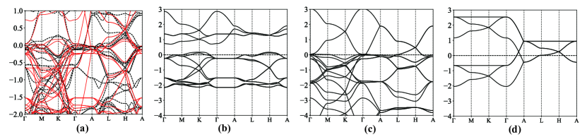
Figure S19: (a) The fitted TB band structures of $\text{MgFe}_{6}\text{Ge}_{6}$ using the decoupled TB model, i.e., combining three Hamiltonians $H_{i=1,2,3}^{[166]}$ defined in LABEL:eq_TB_166_decoupled(red lines), with a comparison with DFT bands in the PM phase (black dashed lines). (b)-(d): Band structure of the decoupled $H_{1}^{[166]}$, $H_{2}^{[166]}$, and $H_{3}^{[166]}$ defined in LABEL:eq_TB_166_decoupled, respectively.

By direct-summing these three Hamiltonians, we arrive at

$$H^{[166]}(\bm{k})=H_{1}^{[166]}(\bm{k})\oplus H_{2}^{[166]}(\bm{k})\oplus H_{3}^{[166]}(\bm{k}),$$ (S6.97)

which gives the final single-particle Hamiltonian

$$\hat{H}_{0}=\sum_{\bm{k}}\sum_{ij}H_{ij}(\bm{k})c^{\dagger}_{\bm{k}i}c_{\bm{k}j},$$ (S6.98)

where the Bloch electron operators $c_{\bm{k}i}$ are defined as the Fourier transform of the following orbital basis

$$( p_{x}@2e_{1},p_{y}@2e_{1},d_{xy}@6i_{1},d_{xy}@6i_{2},d_{xy}@6i_{3},d_{x^{2}-y^{2}}@6i_{1},d_{x^{2}-y^{2}}6i_{2},d_{x^{2}-y^{2}}@6i_{3},$$ (S6.99)

$$p_{x}@2e_{2},p_{y}@2e_{2},d_{xy}@6i_{4},d_{xy}@6i_{5},d_{xy}@6i_{6},d_{x^{2}-y^{2}}@6i_{4},d_{x^{2}-y^{2}}6i_{5},d_{x^{2}-y^{2}}@6i_{6})$$

$$\oplus(p_{z}^{h}@2c_{1},p_{z}^{h}@2c_{2},p_{z}^{h}@2d_{1},p_{z}^{h}@2d_{2},d_{xz}@6i_{1},d_{xz}@6i_{2},d_{xz}@6i_{3},d_{yz}@6i_{1},d_{yz}@6i_{2},d_{yz}@6i_{3},$$

$$d_{xz}@6i_{4},d_{xz}@6i_{5},d_{xz}@6i_{6},d_{yz}@6i_{4},d_{yz}@6i_{5},d_{yz}@6i_{6})$$

$$\oplus(d_{z^{2}}@6i_{1},d_{z^{2}}@6i_{2},d_{z^{2}}@6i_{3},d_{z^{2}}@6i_{4},d_{z^{2}}@6i_{5},d_{z^{2}}@6i_{6}),$$

where $2e_{j}$ and $6i_{j}$ denote the corresponding sites in $2e$ ($z=0.159$) and $6i$ ($z=0.252$) Wyckoff positions defined in Table S2, and $d$ orbitals defined in the local coordinate system in Eq. S2.7. The band structure is shown in Fig. S19, with parameters given in Table S33.

Parameter	$\mu_{p_{xy}^{t}}$	$\mu_{d_{1}}$	$\mu_{d_{2}}$	$t_{d_{1}}^{NN}$	$t_{d_{1}}^{NNN}$	$t_{d_{2}}^{NN}$	$t_{d_{2}}^{NNN}$	$t_{d_{1},d_{2}}^{NN}$	$t_{d_{1},d_{2}}^{NNN}$	$t_{p_{xy}^{t},d_{1}}^{NN}$	$t_{p_{xy}^{t},d_{2}}^{NN}$
Value	-1.8	-1.25	-0.53	0.49	0.03	0.02	0.20	-0.25	-0.16	0.82	1.10
Parameter	$\mu_{p_{z}^{h_{i}}}$	$\mu_{d_{3}}$	$\mu_{d_{4}}$	$t_{d_{3},d_{4}}^{NN}$	$t_{d_{3}}^{NN}$	$t_{d_{4}}^{NN}$	$t_{d_{4}}^{zNN\pm}$	$t_{p_{z}^{h_{i}},d_{4}}^{NN}$	$t_{p_{z}^{h_{i}}}^{NN}$	$t_{p_{z}^{h_{i}},d_{2}}^{NN}$	$\mu_{p_{z}^{t}}$	$t_{p_{z}^{t}}^{NN}$	$t_{p_{z}^{t},d_{3}}^{NN}$
Value	-1.41	-0.88	-0.83	-0.22	-0.23	0.20	0.10	0.77	-0.46	0.31	0.60	0.30	0.45
Parameter	$\mu_{d_{5}}$	$t_{d_{5}}^{NN}$	$t_{d_{5}}^{zNN\pm}$	$\mu_{b}$	$t_{b}^{NN}$	$t_{b}^{zNN\pm}$	$t_{b^{i},d_{5}}^{NN}$	$t_{b^{i},d_{5}}^{NNN}$	$\mu_{s}$	$t_{s,d_{2}}$	$t_{s,d_{3}}$	$t_{s,p_{z}^{t}}$
Value	-1.10	-0.25	0	-0.6	-0.1	0.9	-1.1	0.04	3.07	-0.16	0.31	1.81

Table S33: Onsite energies and hoppings used in the TB model of $\text{MgFe}_{6}\text{Ge}_{6}$ defined in Eq. S6.84, LABEL:Eq:TB2_ham_166, Eq. S6.91. $d_{1}$ to $d_{5}$ denote $d_{xy},d_{x^{2}-y^{2}},d_{xz},d_{yz},d_{z^{2}}$, respectively, $p_{xy}^{t},p_{z}^{t}$ the $p_{x},p_{y}$ and $p_{z}$ orbitals of the trigonal Ge, $p_{z}^{h}$ and $b$ the $p_{z}$ and $sp^{2}$ bonding state of the honeycomb Ge, and $s$ is from Mg. For the simplified $H_{3}^{[166]}(\mathbf{k})$ of $d_{z^{2}}$ only defined in Eq. S6.92, the parameters are $\mu_{d_{5}}=0.54,t_{d_{5}}^{NN}=-0.23,t_{d_{5}}^{zNN}=0.8$. Hoppings colored in blue denote that they can take independent values and can be further fine-tuned, but here we set them to be equal to the values from FeGe for simplicity, modified by the perturbations from Mg.

VI.3 Interaction parameters of $\text{MgFe}_{6}\text{Ge}_{6}$

The interaction parameters are computed for $\text{MgFe}_{6}\text{Ge}_{6}$ using the $d$-full model, i.e., Wannier functions are constructed from $s,p,d$ orbitals of Fe and $s,p$ orbitals of Ge, and exclude only the polarization between $d$ orbitals, as tabulated in Table S34. In Table S35, we list the $O_{h}$-symmetrized onsite Coulomb matrices elements $U_{ij}$ and $J_{ij}$. In Table S36 (Table S37), we list the fitted Coulomb elements $U_{ij}$ and $J_{ij}$ using Slater integrals $F_{0},F_{2},F_{4}$ ($F_{0},F_{2}$ only while fix $F_{4}=0.625F_{2}$). The values of interaction are similar to those of FeGe.

$U_{ij}$	$z^{2}$	$xz$	$yz$	$x^{2}-y^{2}$	$xy$	$J_{ij}$	$z^{2}$	$xz$	$yz$	$x^{2}-y^{2}$	$xy$
$z^{2}$	4.12	2.91	2.97	2.30	2.33			0.57	0.57	0.93	0.94
$xz$		3.97	2.46	2.48	2.52				0.79	0.78	0.80
$yz$			4.12	2.56	2.60					0.79	0.80
$x^{2}-y^{2}$				4.16	3.32						0.46
$xy$					4.30
$U_{ij}^{NN}$	$z^{2}$	$xz$	$yz$	$x^{2}-y^{2}$	$xy$	$U_{ij}^{zNN}$	$z^{2}$	$xz$	$yz$	$x^{2}-y^{2}$	$xy$
$z^{2}$	1.05	1.05	1.07	1.09	1.09			0.91	0.91	0.91	0.91
$xz$		1.05	1.06	1.08	1.09				0.91	0.91	0.91
$yz$			1.10	1.11	1.11					0.90	0.91
$x^{2}-y^{2}$				1.14	1.14						0.90
$xy$					1.15

Table S34: The Coulomb interaction $U_{ij}$ and $J_{ij}$ of $d$ orbitals, and $U_{ij}^{NN}$ and $U_{ij}^{NNN}$ between NN and NNN $d$ in $d-$full model of $\text{MgFe}_{6}\text{Ge}_{6}$. The onsite Hubbard-Kanamori parameters for five $d$ orbitals are $\mathcal{U}=4.13,\mathcal{U}^{\prime}=2.64,\mathcal{J}=0.74$. The averaged NN and NNN interactions are $\overline{U}^{NN}=1.09,\overline{U}^{zNN}=0.91$, with root mean square error being 0.030 and 0.004, respectively. All numbers are in eV.

$U_{ij}$	$z^{2}$	$xz$	$yz$	$x^{2}-y^{2}$	$xy$	$J_{ij}$	$z^{2}$	$xz$	$yz$	$x^{2}-y^{2}$	$xy$
$z^{2}$	4.15	2.99	2.99	2.30	2.30			0.57	0.57	0.92	0.91
$xz$		4.13	2.52	2.53	2.52				0.80	0.80	0.80
$yz$			4.13	2.53	2.52					0.80	0.80
$x^{2}-y^{2}$				4.15	3.23						0.45
$xy$					4.13

Table S35: The Coulomb interaction $U_{ij}$ and $J_{ij}$ of $d$ orbitals for the $d$-full model symmetrized using $O_{h}$ symmetries in $\text{MgFe}_{6}\text{Ge}_{6}$. The root mean square error of the averaged $U_{ij}$ and $J_{ij}$ (error between the fitted values and the DFT values) is 0.153 and 0.050, respectively.

$U_{ij}$	$z^{2}$	$xz$	$yz$	$x^{2}-y^{2}$	$xy$	$J_{ij}$	$z^{2}$	$xz$	$yz$	$x^{2}-y^{2}$	$xy$
$z^{2}$	4.13	2.99	2.99	2.30	2.30			0.57	0.57	0.92	0.92
$xz$		4.13	2.53	2.53	2.53				0.80	0.80	0.80
$yz$			4.13	2.53	2.53					0.80	0.80
$x^{2}-y^{2}$				4.13	3.22						0.45
$xy$					4.13

Table S36: The Coulomb interaction $U_{ij}$ and $J_{ij}$ of $d$ orbitals fitted using Eq. S3.77 in $\text{MgFe}_{6}\text{Ge}_{6}$, where the Slater integrals $F^{0}$, $F^{2}$, and $F_{4}$ are fitted to the full Coulomb matrix $U_{ijkl}$ symmetrized by $O_{h}$ symmetries. The fitted parameters are $F^{0}=2.942,F^{2}=8.842,F^{4}=5.724$. The root mean square error of the fitted $U_{ij}$ and $J_{ij}$ is 0.068 and 0.012, respectively.

$U_{ij}$	$z^{2}$	$xz$	$yz$	$x^{2}-y^{2}$	$xy$	$J_{ij}$	$z^{2}$	$xz$	$yz$	$x^{2}-y^{2}$	$xy$
$z^{2}$	4.12	3.00	3.00	2.29	2.29			0.56	0.56	0.92	0.92
$xz$		4.12	2.53	2.53	2.53				0.80	0.80	0.80
$yz$			4.12	2.53	2.53					0.80	0.80
$x^{2}-y^{2}$				4.12	3.24						0.44
$xy$					4.12

Table S37: The Coulomb interaction $U_{ij}$ and $J_{ij}$ of $d$ orbitals fitted using Eq. S3.77 in $\text{MgFe}_{6}\text{Ge}_{6}$, where the Slater integrals $F^{0}$, $F^{2}$ are fitted to the full Coulomb matrix $U_{ijkl}$ symmetrized by $O_{h}$ symmetries, while $F^{4}=0.625F^{2}$ are fixed. The fitted parameters are $F^{0}=2.942,F^{2}=8.899,F^{4}=5.562$. The root mean square error of the fitted $U_{ij}$ and $J_{ij}$ is 0.069 and 0.013, respectively.

Appendix VII A brief review of the $S$-matrix formalism and flat band theory

In this section, we give a brief review of the $S$-matrix method and flat band theory based on Ref.Călugăru et al. (2022); Ma et al. (2020); Regnault et al. (2022). We summarize the main results here, and rigorous proofs can be found in Ref.Călugăru et al. (2022).

A bipartite crystalline lattice (BCL) is a periodic fermionic lattice with two different sublattices, $L$ and $\tilde{L}$. Assume that $N_{L}$ and $N_{\tilde{L}}$ orbitals per unit cell are placed in the $L$ and $\tilde{L}$ sublattices, respectively, and take $N_{L}\geq N_{\tilde{L}}$ with no loss of generality. The $S$-matrix is the inter-sublattice hopping matrix with dimension $N_{L}\times N_{\tilde{L}}$, denoted by $S(\bm{k})$. The tight-binding (TB) Hamiltonian with only inter-sublattice hoppings has the form

$$H(\bm{k})=\left(\begin{matrix}\bm{0}_{N_{L}}&S(\bm{k})\\ S^{\dagger}(\bm{k})&\bm{0}_{N_{\tilde{L}}}\\ \end{matrix}\right),$$ (S7.100)

where each entry denotes a matrix block, with $\bm{0}_{N}$ being the zero matrix of dimension $N\times N$. This Hamiltonian has chiral symmetry $C$ with the representation matrix

$$D(C)=\text{Diag}(\bm{1}_{N_{L}},-\bm{1}_{N_{\tilde{L}}}),$$ (S7.101)

i.e., $D(C)H(\bm{k})D^{-1}(C)=-H(\bm{k})$. The chiral symmetry enforces the dispersion to be chiral-symmetric, which results in at least $N_{L}-N_{\tilde{L}}$ perfectly flat bands at zero energy. If $\text{rank}(S_{\bm{k}})=r_{s}$, then there will be $2r_{s}$ chirally-symmetric dispersive bands, leading to $N_{L}+N_{\tilde{L}}-2r_{s}$ perfectly flat bands at zero energy.

When intra-sublattice hoppings are added, i.e.,

$$H(\bm{k})=\left(\begin{matrix}A(\bm{k})&S(\bm{k})\\ S^{\dagger}(\bm{k})&B(\bm{k})\\ \end{matrix}\right),$$ (S7.102)

the Hamiltonian is no longer chiral-symmetric. If $A(\bm{k})$ has a $\bm{k}$-independent eigenvalue of multiplicity $n_{a}$ ($n_{a}>N_{\tilde{L}}$), then $H(\bm{k})$ must have $n_{a}-N_{\tilde{L}}$ perfectly flat band, whose energy is not necessarily zero.

Appendix VIII A brief review of quasi-degenerate second-order perturbation theory

In this section, we give a brief summary of the quasi-degenerate second-order perturbation theoryWinkler (2003). Using this method, one can split a Hamiltonian into decoupled subspaces.

Assume we have a solvable Hamiltonian $H_{0}$ with known eigenvalues $\{E_{n}\}$ and eigenvectors $\{\psi_{n}\}$, and $H_{0}$ can be divided into two decoupled (or weakly coupled) subspaces $A$ and $B$. The whole Hamiltonian has the form

$$H=H_{0}+H^{\prime}$$ (S8.103)

where $H^{\prime}$ is assumed to be a perturbation. Divide $H^{\prime}$ into diagonal and off-diagonal parts with respect to $A$ and $B$, i.e., $H^{\prime}=H_{d}^{\prime}+H_{od}^{\prime}$. One can find a similarity transformation $S$, s.t. $\bar{H}=e^{-S}He^{S}$ is diagonal with respect to the $A,B$ subspaces. This means the off-diagonal term $H_{od}^{\prime}$ is perturbed out and $\bar{H}$ becomes block-diagonal.

The most useful formula is the second-order perturbation term, i.e.,

$$S =S^{(1)},$$ (S8.104)

$$\bar{H} =H_{0}+H_{d}^{\prime}+\bar{H}^{(2)},$$

where

$$S^{(1)}_{\alpha\beta} =-\frac{H_{od,\alpha\beta}^{\prime}}{E_{\alpha}-E_{\beta}},$$ (S8.105)

$$\bar{H}^{(2)}_{\alpha\alpha^{\prime}} =\frac{1}{2}\sum_{\beta}H_{od,\alpha\beta}^{\prime}H_{od,\beta\alpha^{\prime}}^{\prime}\left(\frac{1}{E_{\alpha}-E_{\beta}}+\frac{1}{E_{\alpha}^{\prime}-E_{\beta}}\right),$$

in which

$$H_{od,\alpha\beta}^{\prime}=\langle\psi_{\alpha}|H_{od}^{\prime}|\psi_{\beta}\rangle$$ (S8.106)

We give two special cases where the second-order terms have simple analytical forms.

• If

  $$H =\left(\begin{matrix}\mu_{1}\bm{1}_{n}&S\\ S^{\dagger}&\mu_{2}\bm{1}_{m}\\ \end{matrix}\right),$$ (S8.107)

  where $S$ is the S-matrix with shape $(n,m)$. This Hamiltonian can be decoupled into

  $$H_{0} =\left(\begin{matrix}\mu_{1}\bm{1}_{n}&\bm{0}\\ \bm{0}&\mu_{2}\bm{1}_{m}\\ \end{matrix}\right),\quad H_{d}^{\prime}=\bm{0},\quad H_{od}^{\prime} =\left(\begin{matrix}\bm{0}&S\\ S^{\dagger}&\bm{0}\\ \end{matrix}\right).$$ (S8.108)

  Then the second-order perturbed terms have the form if $|\mu_{1}-\mu_{2}|\gg|S|$:

  $$\bar{H}^{(2)}_{1} =\frac{1}{\mu_{1}-\mu_{2}}SS^{\dagger},$$ (S8.109)

  $$\bar{H}^{(2)}_{2} =\frac{1}{\mu_{2}-\mu_{1}}S^{\dagger}S,$$

  $$\Rightarrow\bar{H} =\left(\begin{matrix}\mu_{1}\bm{1}_{n}+\bar{H}^{(2)}_{1}&\bm{0}\\ \bm{0}&\mu_{2}\bm{1}_{m}\bar{H}^{(2)}_{2}\\ \end{matrix}\right).$$

• If

  $$H =\left(\begin{matrix}\mu_{0}\bm{1}_{n_{0}}&S_{1}&S_{2}\\ S_{1}^{\dagger}&\mu_{1}\bm{1}_{n_{1}}&\bm{0}\\ S_{2}^{\dagger}&\bm{0}&\mu_{2}\bm{1}_{n_{2}}\\ \end{matrix}\right),$$ (S8.110)

  where $S_{i}$ is the S-matrix with shape $(n_{0},n_{i})$. This Hamiltonian can be decoupled into

  $$H_{0} =\left(\begin{matrix}\mu_{0}\bm{1}_{n_{0}}&\bm{0}&\bm{0}\\ \bm{0}&\mu_{1}\bm{1}_{n_{1}}&\bm{0}\\ \bm{0}&\bm{0}&\mu_{2}\bm{1}_{n_{2}}\\ \end{matrix}\right),\quad H_{d}^{\prime}=\bm{0},\quad H_{od}^{\prime} =\left(\begin{matrix}\bm{0}&S_{1}&S_{2}\\ S_{1}^{\dagger}&\bm{0}&\bm{0}\\ S_{2}^{\dagger}&\bm{0}&\bm{0}\\ \end{matrix}\right).$$ (S8.111)

  Then the second-order perturbed terms have the following form if $|\mu_{i}-\mu_{0}|\gg|S_{i}|$:

  $$\bar{H}^{(2)}_{0} =\frac{1}{\mu_{0}-\mu_{1}}S_{1}S_{1}^{\dagger}+\frac{1}{\mu_{0}-\mu_{2}}S_{2}S_{2}^{\dagger},$$ (S8.112)

  $$\bar{H}^{(2)}_{1} =\frac{1}{\mu_{1}-\mu_{0}}S_{1}^{\dagger}S_{1},$$

  $$\bar{H}^{(2)}_{2} =\frac{1}{\mu_{2}-\mu_{0}}S_{2}^{\dagger}S_{2},$$

  $$\bar{H}^{(2)}_{12} =\frac{1}{2}\left(\frac{1}{\mu_{1}-\mu_{0}}+\frac{1}{\mu_{2}-\mu_{0}}\right)S_{1}^{\dagger}S_{2},$$

  $$\Rightarrow\bar{H} =\left(\begin{matrix}\mu_{0}\bm{1}_{n_{0}}+\bar{H}^{(2)}_{0}&\bm{0}&\bm{0}\\ \bm{0}&\mu_{1}\bm{1}_{n_{1}}+\bar{H}_{1}^{(2)}&\bar{H}_{12}^{(2)}\\ \bm{0}&\bar{H}_{12}^{(2)\dagger}&\mu_{2}\bm{1}_{n_{2}}+\bar{H}_{2}^{(2)}\\ \end{matrix}\right).$$