Model Agnostic Explainable Selective Regression via Uncertainty Estimation

Abstract

With the wide adoption of machine learning techniques, requirements have evolved beyond sheer high performance, often requiring models to be trustworthy. A common approach to increase the trustworthiness of such systems is to allow them to refrain from predicting. Such a framework is known as selective prediction. While selective prediction for classification tasks has been widely analyzed, the problem of selective regression is understudied. This paper presents a novel approach to selective regression that utilizes model-agnostic non-parametric uncertainty estimation. Our proposed framework showcases superior performance compared to state-of-the-art selective regressors, as demonstrated through comprehensive benchmarking on 69 datasets. Finally, we use explainable AI techniques to gain an understanding of the drivers behind selective regression. We implement our selective regression method in the open-source Python package doubt and release the code used to reproduce our experiments.

1 Introduction

Selective prediction allows machine learning systems to refrain from forecasting, adding the option to abstain whenever the risk of mispredicting is too high. This is an appealing feature for contexts where making wrong predictions can produce relevant harm, such as healthcare or finance. Under this framework, we can distinguish between selective classification and selective regression, similarly to the supervised learning paradigm.

While selective classification has received considerable attention in the past decade, the problem of selective regression remains relatively understudied. Existing approaches for selective regression primarily rely on either deep-learning-based methods Geifman and El-Yaniv, (2019); Jiang et al., (2020) or on the ability to estimate the conditional variance function Zaoui et al., (2020). However, due to the limited scope of empirical evaluations in current state-of-the-art methods, there is a lack of practical insights into the effectiveness and applicability of existing techniques, hindering the development of robust and reliable selective prediction models.

This paper aims to bridge this gap by introducing a novel model-agnostic method for selective regression using non-parametric bootstrap estimators. Our proposed approach offers a robust and reliable solution for abstaining from predicting in regression tasks.

To validate the effectiveness of our selective regression methodology, we conduct extensive empirical evaluations on a set of 69 tabular datasets. This larger-scale benchmarking allows us to gain insights into the performance and generalizability of our proposed approach. Additionally, we incorporate explainable AI methodologies to understand better the factors contributing to the rejection of predictions. By identifying the sources of rejection, we enhance the interpretability of selective regressors, enabling the system users to have accountability over such systems. Our main contributions are:

• a state-of-the-art selective regression method using non-parametric bootstrap to estimate uncertainty;

• an extensive empirical evaluation of selective regression techniques on 69 tabular datasets;

• the application of explainable AI methods to identify the sources of rejection/prediction.

2 Related Work

Prediction with a Reject Option

The idea to allow a machine learning model to abstain in the prediction stage dates back to the 1970s Chow, (1970), when it was introduced for the classification task.

We can distinguish two main frameworks that allow us to learn such a pair: Learning to Reject (LtR) Chow, (1970); Hendrickx et al., (2021) and Selective Classification (SC) El-Yaniv and Wiener, (2010). The former (LtR) requires one to define a class-wise cost function that penalizes mispredictions and rejections Herbei and Wegkamp, (2006); Cortes et al., (2016); Tortorella, (2005); Condessa et al., (2013). The latter (SC) requires instead one to pre-define either a target coverage $c$ or a desired target risk $e$ to achieve. Depending on this choice, a selective classifier can be learnt by either minimizing the risk given the target coverage Geifman and El-Yaniv, (2019); Liu et al., (2019); Huang et al., (2020); Pugnana and Ruggieri, 2023b ; Pugnana and Ruggieri, 2023a ; Feng et al., (2023) or by maximizing coverage given a target risk Geifman and El-Yaniv, (2017); Gangrade et al., (2021). The conditions for equivalence between SC and LtR are studied in  Franc and Průša, (2019).

A few related works have focused on embedding regressors with the reject option. Geifman and El-Yaniv, (2019) proposes a deep learning method called SelNet that, given a target coverage, jointly trains the regressor and the selection function. Jiang et al., (2020) propose the usage of deep ensembles for selective regression in weather forecasting. On the other hand, Zaoui et al., (2020) rely on the Plug-In principle to estimate the optimal selective regressor in a model-agnostic way.

Uncertainty Estimation

Traditionally, uncertainty has been closely associated with standard probability and probabilistic predictions in the statistical realm. However, in the field of machine learning, new challenges have arisen, such as trust, robustness, and safety, necessitating the development of novel methodological approaches Hüllermeier and Waegeman, (2021).

A widely adopted method for uncertainty estimation in machine learning is model averaging Kumar and Srivastava, (2012); Gal and Ghahramani, (2016); Lakshminarayanan et al., (2017). This approach has proven successful in various applications, including monitoring model degradation Mougan and Nielsen, (2023), detecting misclassifications Ren et al., (2019), and addressing adversarial attacks Hendrycks et al., (2021), among others.

In our research, we focus on applying uncertainty to selective regression. Specifically, we extend existing model-agnostic uncertainty frameworks to calculate a confidence function for cases where we abstain from making predictions Kumar and Srivastava, (2012); Mougan and Nielsen, (2023). Additionally, we explore and compare another approach known as conformal prediction, as presented in the work by Kim et al., (2020).

Explainable Reject Option

Explainable AI methods Guidotti et al., (2019) are increasingly used to overcome the difficulty of interpreting AI outputs. Adding explanations to rejections allows for characterizing the areas where the predictor is not confident enough Pugnana, (2023). To the best of our knowledge, the current literature on explaining selective function is limited. Artelt et al., 2022a propose local model agnostic methods to perform such a task; Artelt et al., 2022b use counterfactual explanations to explain the reject option for Learning Vector Quantization (LVQ) algorithms.

In this paper, similarly to  Mougan and Nielsen, (2023), we try to explain the reasons behind the reject option by learning a binary classifier that predicts acceptance/rejection of the original estimator and evaluating its decisions using Shapley Values Lundberg et al., (2020).

3 Methodology

3.1 Selective Regression Framework

Let $X$ and $Y$ be random variables taking values in $\mathcal{X}\subseteq\mathbb{R}^{d}$ and $\mathcal{Y}\subseteq\mathbb{R}$, respectively. A predictor is a function $f\colon\mathcal{X}\to\mathcal{Y}$ and a selection function is a predictor taking values in $\{0,1\}$. We further define, for a predictor $f$ and a selection function $s$, an associated selective predictor $f_{s}$ as

$$f_{s}(X)=\begin{cases}f(X)&\text{if }s(X)=1\\ \emptyset&\text{otherwise},\end{cases}$$ (1)

where $\emptyset$ denotes abstaining from predicting. However, the direct estimation of $s$ can be challenging: for instance, $s$ is not differentiable. Therefore, the selection function can be relaxed by considering an associated confidence function $c_{f}\colon\mathcal{X}\to\mathbb{R}$, sometimes called soft selection Geifman and El-Yaniv, (2017), that measures how likely the predictor $f$ is correct. We can then set a threshold $\tau\in\mathbb{R}$ that defines the minimum confidence for providing a prediction, yielding the associated selection function $x\mapsto\mathds{1}(c_{f}(x)>\tau)$.

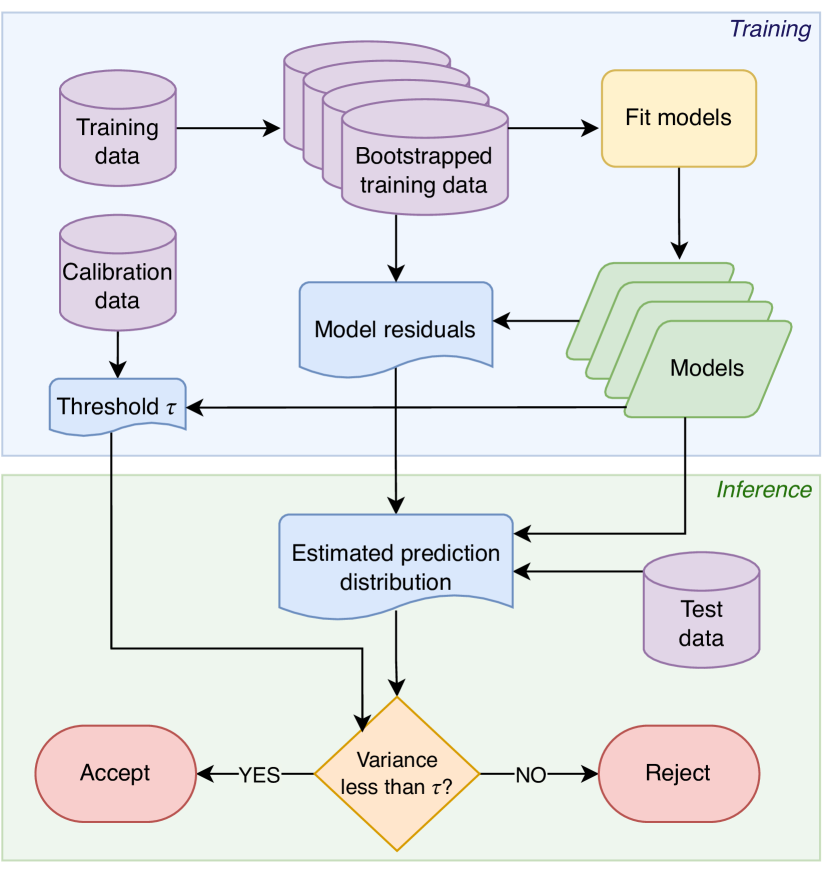
Figure 1: Our DoubtVar selective regression method. Our DoubtInt method is identical, aside from replacing variance with the difference between the 97.5% quantile and the 2.5% quantile.

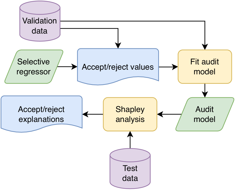
Figure 2: Our explainable selective regression method.

Two important measures are associated with the selective predictor $f_{s}$. The coverage $\texttt{cov}(s):=\mathbb{E}[s(X)]$, being the expected mass probability of the non-rejected region, and the selective risk

$$\texttt{risk}(f,s):=\mathbb{E}[l(f(X),Y)\mid s(X)=1],$$ (2)

being the expected error over accepted instances, where $l\colon\mathcal{Y}\times\mathcal{Y}\to\mathbb{R}$ is a user-defined loss function. Given a target coverage $\alpha$, an optimal selective predictor $f_{s}^{*}$, parameterised by $\theta_{f}$ and $\theta_{s}$, is a solution to

$$\min_{\theta_{f},\theta_{g}}\texttt{risk}(f_{\theta_{f}},s_{\theta_{s}})\quad\text{such that}\quad\texttt{cov}(s_{\theta_{s}})\geq\alpha.$$ (3)

Zaoui et al., (2020) showed that the optimal selective predictor under the mean squared error loss function is obtained by

$$f_{g}^{*}(x)=\begin{cases}f^{*}(x)&\text{if }\sigma^{2}(x)<\tau_{\alpha}\\ \emptyset&\text{otherwise},\end{cases}$$ (4)

where $f^{*}(x):=\mathbb{E}[Y\mid X=x]$ is the regression function, $\sigma^{2}(x):=\mathbb{E}[(Y-f^{*}(x))^{2}\mid X=x]$ is the conditional variance function and $\tau_{\alpha}$ is such that

$$\texttt{cov}(\mathds{1}(\sigma^{2}(X)<\tau_{\alpha}))=\alpha.$$ (5)

In other words, the optimal selective predictor associated with a target coverage $\alpha$ forecasts whenever the variance is below $\tau_{\alpha}$.

Finally, we call calibration the post-training procedure of estimating the threshold $\tau_{\alpha}$ in (4) for the target coverage $\alpha$ specified in (3). This is generally done by estimating the  $1-\alpha$ quantile of the confidence over a held-out calibration dataset Geifman and El-Yaniv, (2019).

3.2 Uncertainty Estimation as a Confidence Function

In this paper, we propose using uncertainty estimation techniques as confidence functions in the sense described in the previous section. We will use a variation of the state-of-the-art doubt uncertainty estimation method Mougan and Nielsen, (2023), which we will briefly describe here. We assume the following relationship between the true values and the model predictions:

$$Y=f(X)+\varepsilon(X)$$ (6)

Here $\varepsilon(X)$ is the combined noise function, which can be split into model variance noise, observation noise and model bias. As the goal is to estimate $\varepsilon(X)$, Mougan and Nielsen, (2023) build a set $C(X)$ consisting of bootstrapped values whose distribution estimates the distribution of $\varepsilon(X)$. Indeed, as this method does not change the asymptotic properties of the prediction interval introduced in Kumar and Srivastava, (2012, Section 4.1.3), the authors show that $C(X)$ converges in distribution to $\varepsilon(X)$ under mild assumptions on $f$ as the number of training samples and bootstraps tend to infinity.

Thus, by adding the model predictions $f(X)$ to the values in $C(X)$, they get an estimation of the prediction distribution. Since convergence in distribution implies convergence of quantiles (see, e.g., Theorem 2A in Parzen, (1980)), this also implies that the resulting prediction intervals built using the quantiles of $C(X)$ are asymptotically correct.

This theoretical justification leads us to consider a potential way to build a selective regressor, as sketched in Figure 1. Namely, we start by fitting the regression model over bootstrapped versions of the training set $(X^{\text{train}},Y^{\text{train}})$ as in Mougan and Nielsen, (2023). Next, we consider the width of the estimated prediction intervals as our confidence function, and we calibrate a selection threshold $\tau$ on a separate calibration set during training. We refer to this method as DoubtInt. The intuition behind DoubtInt is simple: the larger the interval, the more uncertain the prediction, hence abstention is preferable.

Since the optimal selective predictor (4) thresholds the conditional variance function to build the selection function, we also consider a slight variation of DoubtInt by directly using the variance of $C(X)$ rather than the width of the intervals. We refer to this modification as DoubtVar. Once again, the intuition is straightforward: the larger variance of the predictive distribution, the more uncertain the prediction is, making abstaining more likely.

We highlight that both DoubtInt and DoubtVar are completely model-agnostic as they can be used with any off-the-shelf estimator.

3.3 Explainable Selective Regression

Using a confidence function to threshold a rejection of the model’s predictions does not explain why either a given sample was rejected. We propose to solve this open issue by training a classifier to predict the accept/reject decisions of the original regressor model, after which we can perform a Shapley value analysis of the classifier, which can be used to explain why samples are being rejected or accepted. The process is pictured in Figure 2. We start by splitting the data into four parts: training, calibration, validation and test. We use the training and calibration splits to train the selective regressor, as described in the previous subsection and shown in Figure 1. Next, we apply the associated selection function $s_{f}$ on the validation split $X^{\text{validation}}$ and fit an audit model

$$\texttt{audit}\colon\mathcal{X}\to\{0,1\}$$ (7)

on $(X^{\text{validation}},s_{f}(X^{\text{validation}}))$ and compute the Shapley values Lundberg et al., (2020) of audit on the test split.

4 Experiments

We present in this section the experiments to validate our proposed methodology, addressing the following questions:

• Does model-agnostic uncertainty estimation via non-parametric bootstrap achieve state-of-the-art performance for selective regression?

• Does the choice of different regression algorithms affect the results from Q1?

• Can we characterize the features that led to the rejection decision of a single instance?

4.1 Experimental Settings

Data

For Q1 and Q2, we consider 69 tabular regression datasets from existing regression benchmarks Olson et al., (2017); Grinsztajn et al., (2022). Data include applications from different domains, such as finance, healthcare and natural sciences. To limit computational time, we exclude large datasets from the current study, i.e. $n\geq 100,000$, with $n$ representing the dataset size. We additionally exclude datasets with a size $n\leq 100$, to have enough data to test different target coverages. We further detail the datasets’ characteristics in Table A1 of the appendix. We apply one-hot encoding to categorical variables and employ feature and target variable Min-Max normalisation to account for the varying ranges in the feature and target distributions. We run experiments using five different seeds and consider the average results over these runs.

For Q3, we consider the popular House Prices regression dataset to illustrate how our explainable selective regression method works. The task is to predict the selling price of a given property, with a subset of the seven most predictive features.

Baselines

As we employ tabular datasets, in which tree-based methods such as gradient boosting have been shown to achieve better performance Gorishniy et al., (2021); Grinsztajn et al., (2022), we compare our approach to other non-deep learning model-agnostic methods from the literature. The baselines we consider are:

Plug-In, a model-agnostic method introduced by Zaoui et al., (2020). PlugIn works as follows. Given a target coverage $\alpha$, training samples $(X^{\text{train}},Y^{\text{train}})$ and unlabelled calibration samples $X^{\text{cal}}\sim P_{X}$, it firstly estimates the selective regressor by fitting a regression function $\hat{f}$ on $(X^{\text{train}},Y^{\text{train}})$. Next, the training residuals $\varepsilon^{\text{train}}:=(Y^{\text{train}}-\hat{f}(X^{\text{train}}))^{2}$ are computed. We then fit another regression function $\hat{g}$ on $(X^{\text{train}},\varepsilon^{\text{train}})$ and compute the predicted residual values $\hat{g}(X^{\text{train}})$ of the calibration set $X^{\text{cal}}$. Lastly, we use the predicted residuals to calibrate the selective regressor;

SCross, an adaptation of the algorithm by  Pugnana and Ruggieri, 2023b to selective regression. SCross mitigates overfitting concerns of PlugIn Kennedy, (2020) by applying cross-validation to obtain validation residuals of $\hat{f}$ instead of training residuals. This is done by splitting the training set into $K$ folds, training the regressor on $K-1$ folds and computing residuals over the final $K$’th fold. We repeat this procedure $K$ times and use the residuals from all $K$ iterations to fit the $\hat{g}$ function. Finally, similarly to PlugIn, SCross calibrates the selective regressor over the unlabeled set $X^{\text{cal}}$;

MAPIE, a method that estimates the uncertainty around predictions using the conformal prediction technique from Kim et al., (2020); Romano et al., (2019); Xu and Xie, (2021). We first fit the regressor over the training set to build the selective regressor. We then use the $\text{CV}^{+}$ technique Barber et al., (2020) with $K=5$ to produce prediction sets at 95%, and we consider the width of the provided prediction interval as a proxy for the selection function $s$ (the larger the interval, the more likely the rejection). We finally calibrate the selective regressor over an unlabeled calibration dataset $X^{\text{cal}}$;

GoldCase, an Oracle implementation with access to $Y$ labels. This method rejects instances whose residual value is above the $\alpha$-th percentile. GoldCase provides an upper bound to the performance of all the other baselines.

Hyperparameters

For Q1, we consider XGBoost Chen and Guestrin, (2016) as the base algorithm since it achieves state-of-the-art performance in many tasks Grinsztajn et al., (2022); Borisov et al., (2021).

For Q2, we also consider LightGBM and scikit-learn implementations of LinearRegression, DecisionTree and RandomForest. Hyperparameters are set to default API values. For DoubtVar and DoubtInt, we set the number of bootstraps to the default value $\sqrt{n_{\text{train}}}$, with $n_{\text{train}}$ representing the training set size. For SCross and Mapie, we set the number of folds to their default value $K=5$.

Metrics

For Q1 and Q2, we compute actual coverage denoted as $\widehat{\texttt{cov}}(s)$, i.e. the sample counterpart of $\texttt{cov}(s)$. We use actual coverage to check whether existing methods satisfy the coverage constraint. Ideally, we want the difference $\texttt{cov}(s)-\widehat{\texttt{cov}}(s)$ to be negative; i.e., that the predicted coverage is no less than the target coverage. Since small violations could occur in practice, we consider as a coverage violation the following metric:

$$\texttt{CovSat}(s):=\mathds{1}{}(\texttt{cov}(s)-\widehat{\texttt{cov}}(s)\geq\varepsilon)$$

where $\varepsilon$ is set to $0.05$ to account for reasonably small violations. We measure performance using the percentage decrease of Mean Squared Error, i.e.

$$\Delta\texttt{MSE}(h,g,c):=\frac{\texttt{MSE}(h,g,c)}{\texttt{MSE}(h,g,1)}-1,$$

where $\texttt{MSE}(h,g,c)$ is the Mean Squared Error computed over accepted instances at desired coverage $c$ and $\texttt{MSE}(h,g,1)$ is the Mean Squared Error on the full sample. The lower $\Delta\texttt{MSE}$, the more the model can improve its performance once we allow abstention. This allows for a relative comparison of performances across multiple datasets and coverages. Moreover, since the lower the coverage, the lower the expected MSE, we need to account for coverage violations to guarantee a fair comparison across methods. Regarding this aspect, if $\texttt{CovSat}(s)=0$, we set $\Delta\texttt{MSE}=0$ to avoid rewarding those methods that improve performance by over-rejecting instances.

Hardware

We use a 96 cores machine with Intel(R) Xeon(R) Gold 6342 CPU @ 2.80GHz and two NVIDIA RTX A6000, OS Ubuntu 20.04.4 for all the experiments. The experiments took roughly two days on the server, with an estimated $CO_{2}$ consumption of $\sim 7.5kg$ according to codecarbon Lacoste et al., (2019); Courty et al., (2023).

4.2 Q1: Evaluating Bootstrap Uncertainty as a Confidence Function

In this subsection, we provide results when evaluating DoubtInt and DoubtVar as methods to perform selective regression.

Setup

We randomly split each dataset into a $60/20/20$ training/calibration/test split and train the selective regressor on the training set. We then choose different target coverages $c\in\{.99,.95,.90,.85,.80,.75,.70,.65,.60..55,.50\}$, and calibrate a selection function over the calibration set for each of these. Lastly, we compute CovSat and $\Delta\texttt{MSE}$ of the calibrated selection functions over accepted instances on the test set.

Results

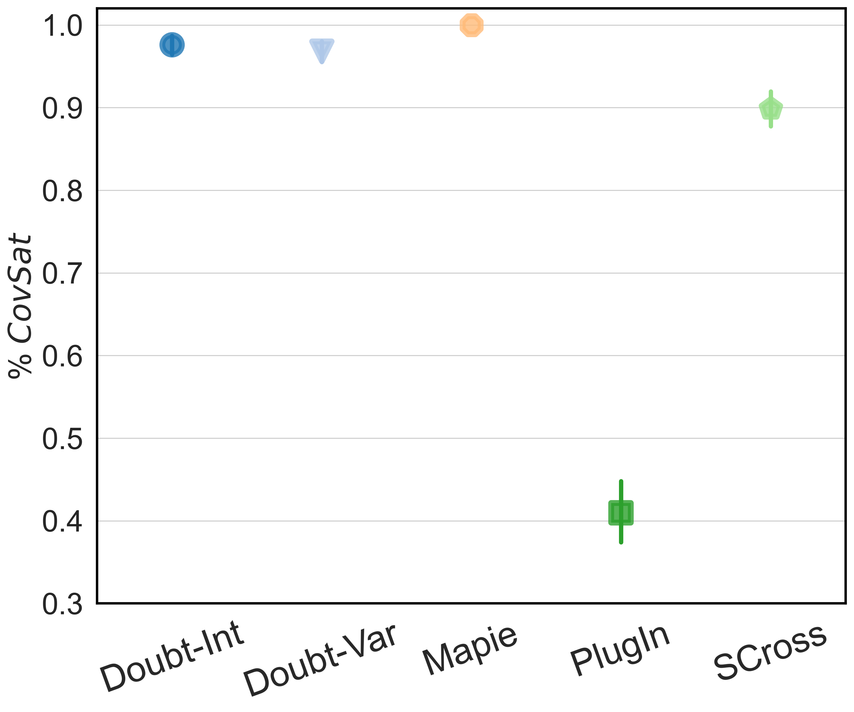
(a) % $\texttt{CovSat}=1$ for different baselines (higher is better)

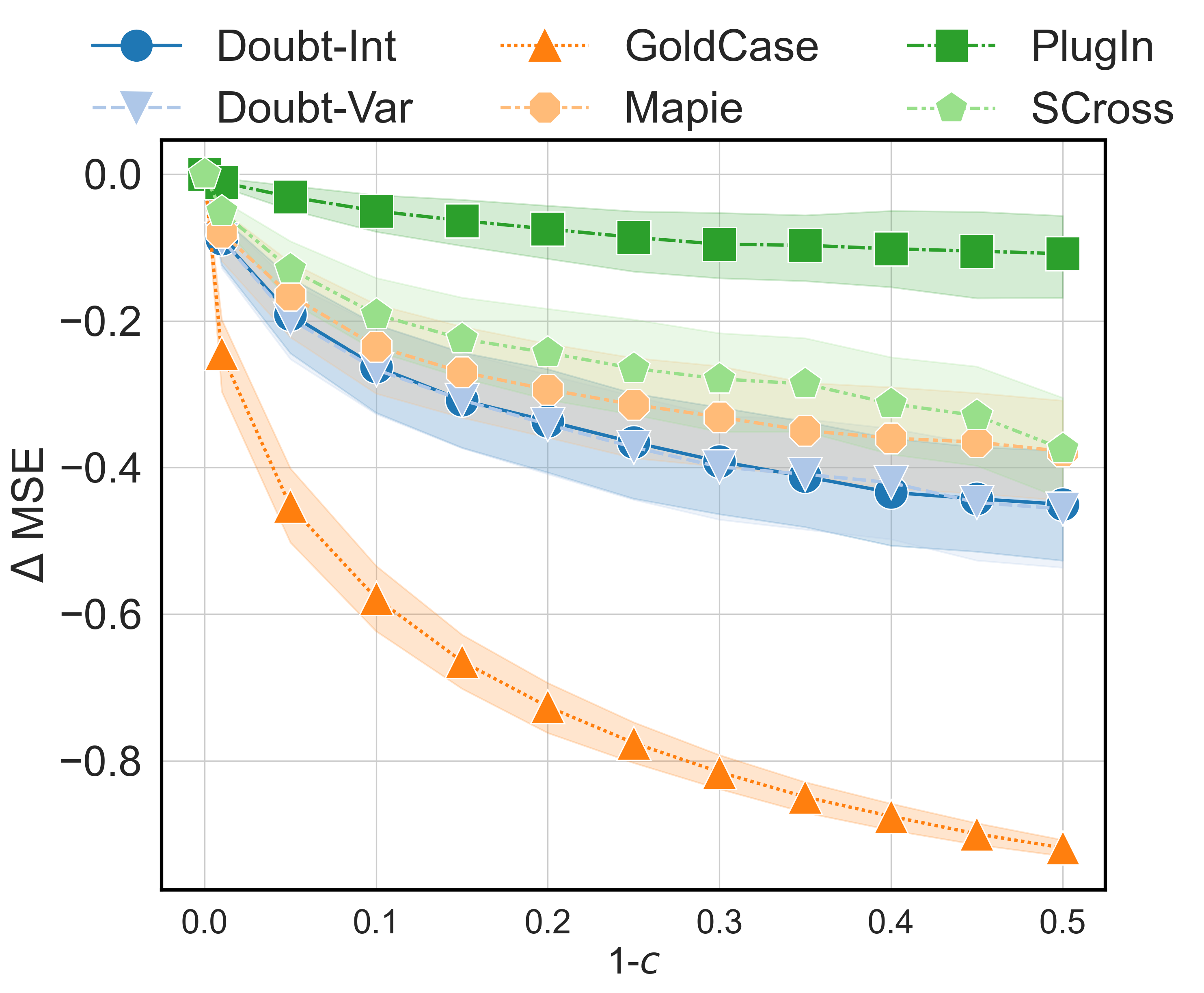
(b) $\Delta\texttt{MSE}$ for reject rate ($1-c$) levels (lower is better).

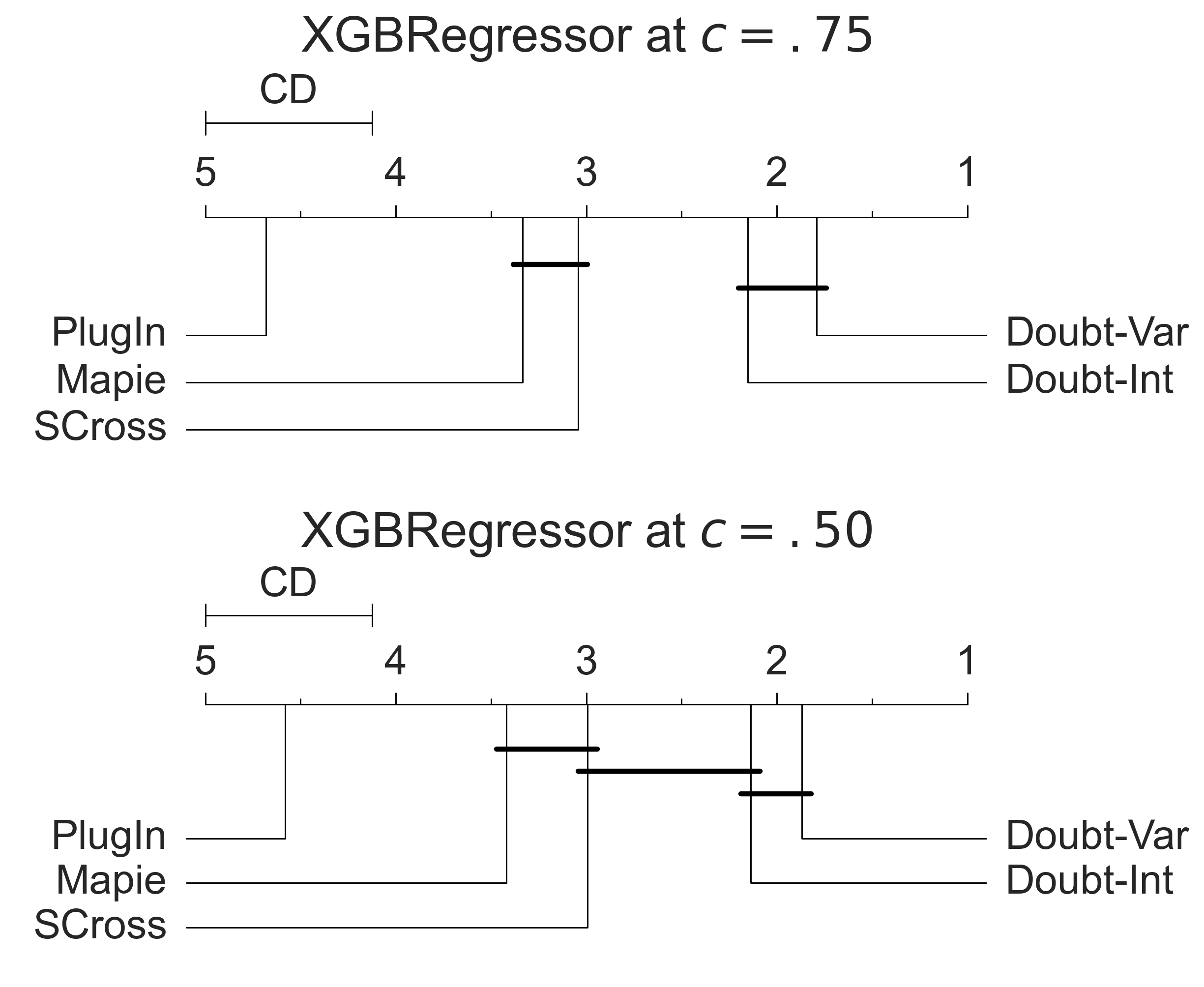
(c) CD plots at $c=.75$ and $c=.50$.

Figure 3: The Q1 experiments, showing the results on selected datasets using XGBoost. In the Critical Difference plot in (c), the differences are statistically significant whenever the bold lines do not intersect multiple baselines.

Figure 3(a) reports the percentage of times the baselines achieve $\texttt{CovSat}=1$ over our experiments when using XGBoost as the base regressor. We can see that the only method with large coverage violations is PlugIn, with a percentage of $\sim 41\%$ of the experiments. This happens as the selective regressor overfit data, failing to properly estimate the conditional variance function. A large part of coverage violations occurs on small datasets ($n<1,000$), where PlugIn achieves desired coverage only $8.8\%$ of the time. On the other hand, all the other methods show a percentage of roughly $\sim 90\%$, with Mapie achieving $100\%$ of satisfied constraints.

Figure 3(b) shows the average $\Delta\texttt{MSE}$ values for the different baseline methods and coverages over the analyzed datasets. Due to space limits, we report results at dataset level in the appendix. For lower coverages, DoubtInt and DoubtVar reach the best performance, with an average drop in MSE of $\sim.45\%$ and $\sim 45.6\%$, respectively, at $c=.5$. PlugIn achieves the worst performance, with an average drop at $c=.5$ of $\sim 10.8\%$, which is more than three times less the drop achieved by DoubtVar and DoubtInt.

To evaluate the statistical significance of our results, we use the Nemenyi post-hoc test at a 95% significance level  Demsar, (2006). Figure 3(c) provides the Critical Difference (CD) plots resulting from the tests at $c=.75$ and $c=.5$ (the median and minimum values of target coverages). At $c=.75$, the difference between the bootstrap uncertainty estimation strategies and all the other baselines is statistically significant. On the other hand, the performance of DoubtVar and DoubtInt is not statistically distinguishable. This result also holds when decreasing the coverage further, with DoubtVar and DoubtInt outperforming other methods and still not different from each other in a statistically significant sense. Hence, experimental evidence seems to support the usage of bootstrap uncertainty estimation as a reliable way to perform selective regression, answering Q1 in the positive.

4.3 Q2: Evaluating the Regressor Choice

In this subsection, we investigate how the choice of the base regressor affects the results of bootstrap-based methods and other model-agnostic baselines.

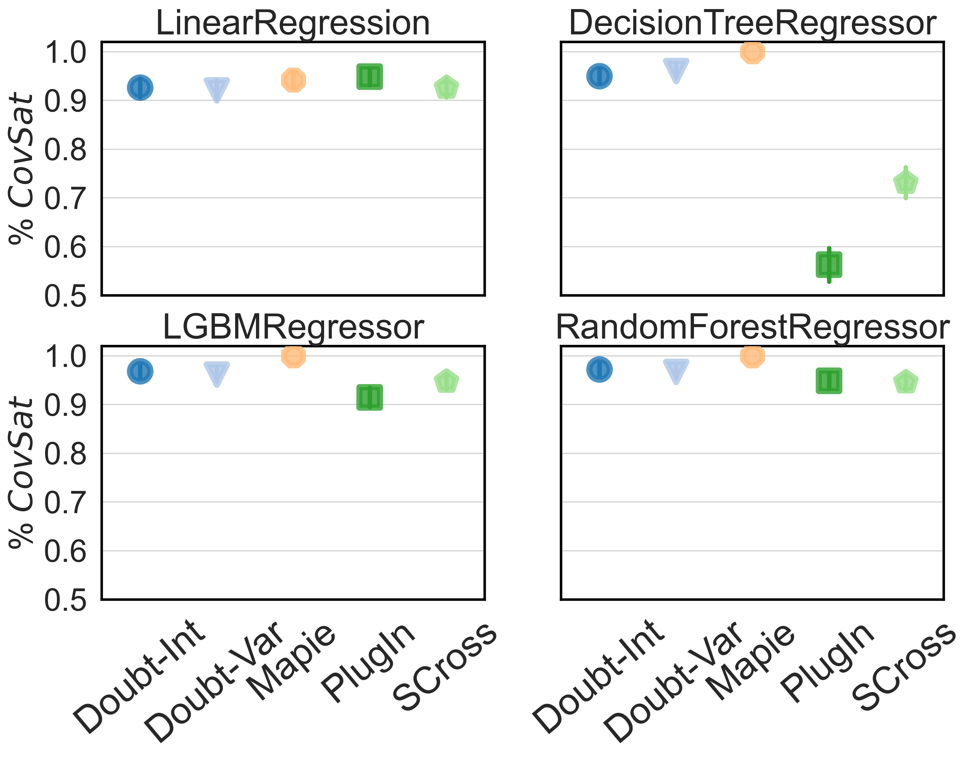
(a) % $\texttt{CovSat}=1$ for different regressors.

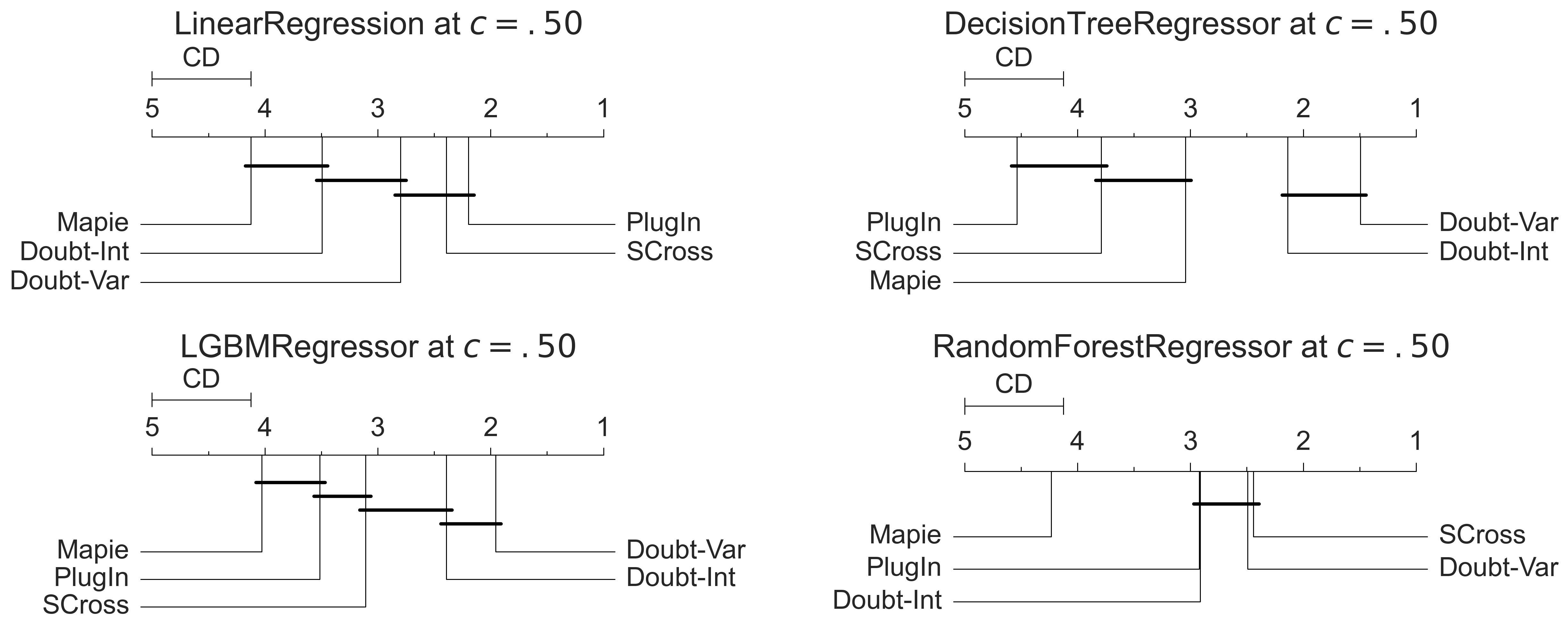
(b) CD plot for different regressors.

Figure 4: The Q2 experiments, comparing the performance when varying the underlying regression algorithm.

Setup

We follow the same setup of Q1, and consider the base regressors presented in the hyperparameters paragraph.

Results

Figure 4(a), displays the percentage of $\texttt{CovSat}=1$ for the different algorithms analyzed. We see that the only algorithm where large coverage violations occur is DecisionTree, where PlugIn and SCross satisfy coverage constraints on $\sim 56.3$% and $\sim 73.1$% of the experiments, respectively. The coverage is satisfied for all the other regression algorithms in roughly $90$% of the cases.

To evaluate the robustness of bootstrap-based methods, we run the Nemenyi post-hoc test using $\Delta\texttt{MSE}$ for the different regression algorithms, and we report the CD plots at the minimal coverage $c=.5$ in Figure 4(b). When considering LinearRegression, PlugIn is ranked first, even though with no statistically significant difference with respect to SCross and DoubtVar. When focusing on the DecisionTree regressor, DoubtVar and DoubtInt are ranked first and second, respectively, with statistically significant differences from the other baselines not based on bootstrap uncertainty estimation.

When evaluating LightGBM, DoubtVar and DoubtInt achieve the top-2 positions. However, DoubtInt is not statistically different from SCross. On the other hand, when considering RandomForest, all the methods, aside from MAPIE, are indistinguishable.

These results suggest that our bootstrap-based approaches help improve performance. In particular, our method is preferable when we consider regression algorithms prone to overfitting, such as single decision trees. This is because PlugIn learns the selection function on the same data used to build the regression function, leading to potential over-fitting concerns Kennedy, (2020). Thus, the findings of our analysis constitute a negative answer to Q2, since DoubtVar is always as good or better than previous SOTA methods.

4.4 Q3: Explainable Model Agnostic Selective Regression

In this section, we show how our methodology of explainable selective regression, as illustrated in Figure 2, can assist users in auditing rejection decisions.

Setup

Since this section aims to show how we can characterize the selection strategy, we consider an illustrative setup inspired by previous work on model degradation by  Mougan and Nielsen, (2023). Given a dataset, we add a randomly generated feature $X_{Random}$ to generate a feature independent of target variable $Y$. We then randomly split data according to a 25/25/25/25 proportion between the training, calibration, validation and test set. We use training and calibration sets to learn a DoubtVar selective regressor on the extended feature space, using XGBoost algorithm as the base model. We train an audit model on the validation set, following the steps described in the methodology section. To build the audit model, we employ the default sklearn implementation of LogisticRegression and set a target coverage $c=.80$. Due to space limits, we provide results for different algorithm choices in Appendix Table A2.

Subsequently, we induce a distribution shift to force the model into rejecting samples that would have otherwise been accepted. To achieve this, we isolate the accepted instances from the test set. Then, iteratively, for every feature within the expanded feature space, we perturb the variable distribution through Gaussian noise $\varepsilon\sim\mathcal{N}(5,1)$.

We use the full conditional SHAP technique to estimate the Shapley values distribution of the audit model for both the perturbed and the non-perturbed case. This is done because such a technique respects the correlations among the input features, so if the model depends on one input and that input is correlated with another, both get some credit for the model’s behavior Lundberg and Lee, (2017); Lundberg et al., (2018). We then compute the Wasserstein distance Kantorovich, (1960); Vaserstein, (1969) between the univariate Shapley value distribution of the audit model in both non-perturbated and perturbated cases to measure how much the perturbations affect explanations distributions. We finally consider perturbations occurring at the same time on $X_{Random}$ and $X_{GrLivArea}$ (one of the most predictive features) to show how one can characterize the selection function through a visualization of the explanations distributions.

Results

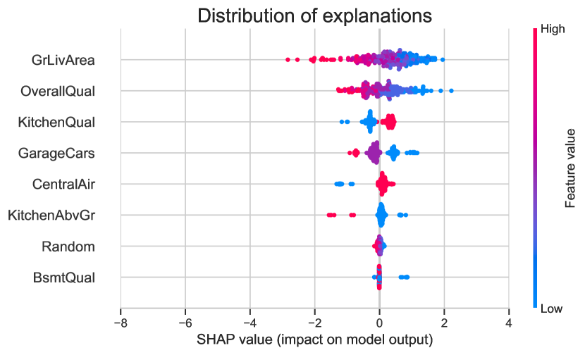
Figure 5: The plot illustrates two features, $X_{\text{Random}}$ and $X_{\text{GrLiveArea}}$, of the House Regression dataset, being simultaneously shifted. The top image displays local explanations for the original distributions, while the bottom image shows the shifted features.

Feature	Wasserstein Distance
GrLivArea	$5.38\pm 0.06$
OverallQual	$3.83\pm 0.03$
CentralAir	$2.32\pm 0.02$
KitchenAbvGr	$1.75\pm 0.02$
BsmtQual	$0.76\pm 0.01$
KitchenQual	$0.66\pm 0.01$
GarageCars	$0.463\pm 0.003$
Random	$0.175\pm 0.001$

Table 1: Wasserstein distance over the Shapley distributions of the predicted samples when univariate shifting the features for the House Regression dataset (higher is a more impactful shift). Results are reported as the average $\pm$ standard deviation over different runs.

Table 1 provides the Wasserstein distance obtained when shifting the features individually. We can see that the distribution of the explanations for the random variable $X_{random}$ is less affected by the perturbation, as low Wasserstein implies more similar distributions. On the contrary, the Shapley distribution of the selection function explanations shifts more substantially for features with more predictive power to determine the acceptance/rejection.

We further illustrate the mechanism behind the selective function in Figure 5, where we plot the Shapley distributions when considering a shift occurring simultaneously in $X_{Random}$ and $X_{GrLiveArea}$. The top image represents the Shapley values distribution when no shift has occurred over the accepted instances, while the bottom image depicts the distribution in the shifted scenario. We notice that the perturbation in $X_{GrLiveArea}$ shifts Shapley distribution towards negative values, decreasing the chances for instances to be accepted by the final selective regressor. This aligns with our desiderata, as we would like to abstain more when evaluating instances belonging to the feature space’s unexplored (hence more uncertain) areas. On the other hand, the shift in $X_{\text{Random}}$ has a less impact on the distribution of the Shapley values, showing that non-relevant features shift do not affect the acceptance/rejection decision. Thus, we can positively answer to Q3, as our explainable selective regression methodology allows us to describe the key drivers of the selection function.

5 Conclusions

This paper addresses the understudied problem of selective regression, introducing a novel method based on the state-of-the-art uncertainty estimation technique by Mougan and Nielsen, (2023). This allows any regressor to abstain from making predictions when facing high uncertainty. Our method is theoretically grounded and completely model-agnostic. We provide an extensive empirical evaluation over 69 datasets and different regression algorithms, showing how our approach is as good or better than competing methods and is especially useful when over-fitting concerns might occur. Finally, we use Shapley values, in conjunction with the proposed uncertainty-based selective regressor, to identify which features are driving rejection, providing a simple-yet-effective method to validate the selection function.

Limitations:

We confine our analysis to datasets with sizes ranging from $100<n<100,000$. Within this range, our techniques exhibit enhancements over prevailing methods across a spectrum of base algorithms. Moreover, our benchmark exclusively encompasses non-deep learning methods, which facilitates expedited algorithm training through bootstrap samples. The extension of our approach to larger deep-learning models could entail heightened complexity due to potential computational intensiveness. Furthermore, our explainable AI approach rests on the estimation of Shapley values, and varying choices in models or Shapley value approximations may yield disparate outcomes.

Reproducibility Statement

To ensure reproducibility of our results, we make the data, data preparation routines, code repositories, and methods publicly available. Our methods will be included in the open-source Python package doubt.

Supplementary Material for Model Agnostic Explainable Selective Regression via Uncertainty Estimation

Appendix A Supplementary Material for Model Agnostic Explainable Selective Regression via Uncertainty Estimation

A.1 Data Details

We provide in Table A1 the set of data employed in our analysis. We report the name of the dataset, the link to the original repository, the number of training instances and the number of features employed in the regression task.

Table A1: Dataset Details

Dataset	Link	Training Size	Feature Space Dim.
1027_ESL	https://epistasislab.github.io/pmlb/profile/1027“˙ESL.html	292	4
1028_SWD	https://epistasislab.github.io/pmlb/profile/1028“˙SWD.html	600	10
1029_LEV	https://epistasislab.github.io/pmlb/profile/1029“˙LEV.html	600	4
1030_ERA	https://epistasislab.github.io/pmlb/profile/1030“˙ERA.html	600	4
1193_BNG_lowbwt	https://epistasislab.github.io/pmlb/profile/1193“˙BNG“˙lowbwt.html	18,662	9
1199_BNG_echoMonths	https://epistasislab.github.io/pmlb/profile/1199“˙BNG“˙echoMonths.html	10,497	9
197_cpu_act	https://epistasislab.github.io/pmlb/profile/197“˙cpu“˙act.html	4,915	21
201_pol	https://epistasislab.github.io/pmlb/profile/201“˙pol.html	9,000	48
207_autoPrice	https://epistasislab.github.io/pmlb/profile/207“˙autoPrice.html	95	15
210_cloud	https://epistasislab.github.io/pmlb/profile/210“˙cloud.html	64	5
215_2dplanes	https://epistasislab.github.io/pmlb/profile/215“˙2dplanes.html	24,460	10
218_house_8L	https://epistasislab.github.io/pmlb/profile/218“˙house“˙8L.html	13,670	8
225_puma8NH	https://epistasislab.github.io/pmlb/profile/225“˙puma8NH.html	4,915	8
227_cpu_small	https://epistasislab.github.io/pmlb/profile/227“˙cpu“˙small.html	4,915	12
229_pwLinear	https://epistasislab.github.io/pmlb/profile/229“˙pwLinear.html	120	10
230_machine_cpu	https://epistasislab.github.io/pmlb/profile/230“˙machine“˙cpu.html	125	6
294_satellite_image	https://epistasislab.github.io/pmlb/profile/294“˙satellite“˙image.html	3,861	36
344_mv	https://epistasislab.github.io/pmlb/profile/344“˙mv.html	24,460	10
4544_GeographicalOriginalofMusic	https://epistasislab.github.io/pmlb/profile/4544“˙GeographicalOriginalofMusic.html	635	117
503_wind	https://epistasislab.github.io/pmlb/profile/503“˙wind.html	3,944	14
505_tecator	https://epistasislab.github.io/pmlb/profile/505“˙tecator.html	144	124
519_vinnie	https://epistasislab.github.io/pmlb/profile/519“˙vinnie.html	228	2
522_pm10	https://epistasislab.github.io/pmlb/profile/522“˙pm10.html	300	7
529_pollen	https://epistasislab.github.io/pmlb/profile/529“˙pollen.html	2,308	4
537_houses	https://epistasislab.github.io/pmlb/profile/537“˙houses.html	12,384	8
547_no2	https://epistasislab.github.io/pmlb/profile/547“˙no2.html	300	7
556_analcatdata_apnea2	https://epistasislab.github.io/pmlb/profile/556“˙analcatdata“˙apnea2.html	285	3
557_analcatdata_apnea1	https://epistasislab.github.io/pmlb/profile/557“˙analcatdata“˙apnea1.html	285	3
560_bodyfat	https://epistasislab.github.io/pmlb/profile/560“˙bodyfat.html	151	14
564_fried	https://epistasislab.github.io/pmlb/profile/564“˙fried.html	24,460	10
574_house_16H	https://epistasislab.github.io/pmlb/profile/574“˙house“˙16H.html	13,670	16
581_fri_c3_500_25	https://epistasislab.github.io/pmlb/profile/581“˙fri“˙c3“˙500“˙25.html	300	25
582_fri_c1_500_25	https://epistasislab.github.io/pmlb/profile/582“˙fri“˙c1“˙500“˙25.html	300	25
584_fri_c4_500_25	https://epistasislab.github.io/pmlb/profile/584“˙fri“˙c4“˙500“˙25.html	300	25
586_fri_c3_1000_25	https://epistasislab.github.io/pmlb/profile/586“˙fri“˙c3“˙1000“˙25.html	600	25
589_fri_c2_1000_25	https://epistasislab.github.io/pmlb/profile/589“˙fri“˙c2“˙1000“˙25.html	600	25
592_fri_c4_1000_25	https://epistasislab.github.io/pmlb/profile/592“˙fri“˙c4“˙1000“˙25.html	600	25
598_fri_c0_1000_25	https://epistasislab.github.io/pmlb/profile/598“˙fri“˙c0“˙1000“˙25.html	600	25
605_fri_c2_250_25	https://epistasislab.github.io/pmlb/profile/605“˙fri“˙c2“˙250“˙25.html	150	25
620_fri_c1_1000_25	https://epistasislab.github.io/pmlb/profile/620“˙fri“˙c1“˙1000“˙25.html	600	25
633_fri_c0_500_25	https://epistasislab.github.io/pmlb/profile/633“˙fri“˙c0“˙500“˙25.html	300	25
643_fri_c2_500_25	https://epistasislab.github.io/pmlb/profile/643“˙fri“˙c2“˙500“˙25.html	300	25
644_fri_c4_250_25	https://epistasislab.github.io/pmlb/profile/644“˙fri“˙c4“˙250“˙25.html	150	25
653_fri_c0_250_25	https://epistasislab.github.io/pmlb/profile/653“˙fri“˙c0“˙250“˙25.html	150	25
658_fri_c3_250_25	https://epistasislab.github.io/pmlb/profile/658“˙fri“˙c3“˙250“˙25.html	150	25
663_rabe_266	https://epistasislab.github.io/pmlb/profile/663“˙rabe“˙266.html	72	2
665_sleuth_case2002	https://epistasislab.github.io/pmlb/profile/665“˙sleuth“˙case2002.html	88	6
666_rmftsa_ladata	https://epistasislab.github.io/pmlb/profile/666“˙rmftsa“˙ladata.html	304	10
678_visualizing_environmental	https://epistasislab.github.io/pmlb/profile/678“˙visualizing“˙environmental.html	66	3
690_visualizing_galaxy	https://epistasislab.github.io/pmlb/profile/690“˙visualizing“˙galaxy.html	193	4
695_chatfield_4	https://epistasislab.github.io/pmlb/profile/695“˙chatfield“˙4.html	141	12
712_chscase_geyser1	https://epistasislab.github.io/pmlb/profile/712“˙chscase“˙geyser1.html	133	2
abalone	https://www.openml.org/search?type=data&status=active&id=42726	2,506	9
bikes	https://www.openml.org/search?type=data&status=active&id=42712	10,427	16
brazilian_houses	https://www.openml.org/search?type=data&status=active&id=42688	6,415	48
diamonds	https://www.openml.org/search?type=data&status=active&id=42225	32,364	23
elevators	https://www.openml.org/search?type=data&status=active&id=216	9,959	18
house_sales	https://www.openml.org/search?type=data&status=active&id=42731	12,967	21
mercedes	https://www.openml.org/search?type=data&status=active&id=42570	2,525	555
miami	https://www.openml.org/search?type=data&status=active&id=43093	8,359	16
nikuradse_1	https://epistasislab.github.io/pmlb/profile/nikuradse“˙1.html	217	2
nikuradse_2	https://epistasislab.github.io/pmlb/profile/nikuradse“˙2.html	217	1
seattle	https://www.openml.org/search?type=data&status=active&id=42496	31,414	293
soil	https://www.openml.org/search?type=data&status=active&id=688	5,184	4
sulfur	https://www.openml.org/search?type=data&status=active&id=23515	6,048	5
superconduct	https://www.openml.org/search?type=data&status=active&id=43174	12,757	81
supreme	https://www.openml.org/search?type=data&status=active&id=504	2,431	7
topo21	https://www.openml.org/search?type=data&status=active&id=422	5,331	266
y_prop	https://www.openml.org/search?type=data&status=active&id=416	5,331	251

A.2 Additional Results for Q3

To show how the performance of the audit model depends on the base regressor and the classifier algorithm employed, Table A2 reports the Area Under the ROC Curve (AUC) score on the test set achieved by different audit models. The results show that the best fit is achieved when pairing XGBoost with a LogisticRegrssion. At the same time, the worst performance is obtained when using the LinearRegression algorithm and the LogisticRegression.

Table A2: AUC obtained by the audit model on predicting which instances will be rejected by DoubtVar on the House Regression dataset.

	Estimator
Auditor	DecisionTree	XGBoost	LinearRegression	RandomForest
DecisionTreeClassifier	0.872	0.892	0.654	0.872
XGBoostClassifier	0.888	0.902	0.671	0.896
KNeighborsClassifier	0.868	0.891	0.694	0.917
LogisticRegression	0.897	0.935	0.609	0.884
MLPClassifier	0.903	0.876	0.673	0.889
RandomForestClassifier	0.86	0.91	0.681	0.884

References

- (1) Artelt, A., Brinkrolf, J., Visser, R., and Hammer, B. (2022a). Explaining reject options of learning vector quantization classifiers. In IJCCI, pages 249–261. SCITEPRESS.
- (2) Artelt, A., Visser, R., and Hammer, B. (2022b). Model agnostic local explanations of reject. In ESANN.
- Barber et al., (2020) Barber, R. F., Candes, E. J., Ramdas, A., and Tibshirani, R. J. (2020). Predictive inference with the jackknife+.
- Borisov et al., (2021) Borisov, V., Leemann, T., Seßler, K., Haug, J., Pawelczyk, M., and Kasneci, G. (2021). Deep neural networks and tabular data: A survey. CoRR, abs/2110.01889.
- Chen and Guestrin, (2016) Chen, T. and Guestrin, C. (2016). Xgboost: A scalable tree boosting system. In KDD, pages 785–794. ACM.
- Chow, (1970) Chow, C. K. (1970). On optimum recognition error and reject tradeoff. IEEE Trans. Inf. Theory, 16(1):41–46.
- Condessa et al., (2013) Condessa, F., Bioucas-Dias, J. M., Castro, C. A., Ozolek, J. A., and Kovacevic, J. (2013). Classification with reject option using contextual information. In ISBI, pages 1340–1343. IEEE.
- Cortes et al., (2016) Cortes, C., DeSalvo, G., and Mohri, M. (2016). Boosting with abstention. In NIPS, pages 1660–1668.
- Courty et al., (2023) Courty, B., Schmidt, V., Goyal-Kamal, MarionCoutarel, Feld, B., Lecourt, J., SabAmine, Léval, M., Cruveiller, A., Zhao, F., Joshi, A., Bogroff, A., de Lavoreille, H., Laskaris, N., LiamConnell, Saboni, A., Blank, D., Wang, Z., Catovic, A., alencon, JPW, MinervaBooks, SangamSwadiK, brotherwolf, and Pollard, M. (2023). mlco2/codecarbon: v2.2.7.
- Demsar, (2006) Demsar, J. (2006). Statistical comparisons of classifiers over multiple data sets. J. Mach. Learn. Res., 7:1–30.
- El-Yaniv and Wiener, (2010) El-Yaniv, R. and Wiener, Y. (2010). On the foundations of noise-free selective classification. J. Mach. Learn. Res., 11:1605–1641.
- Feng et al., (2023) Feng, L., Ahmed, M. O., Hajimirsadeghi, H., and Abdi, A. H. (2023). Towards better selective classification. In ICLR.
- Franc and Průša, (2019) Franc, V. and Průša, D. (2019). On discriminative learning of prediction uncertainty. In ICML, volume 97 of Proceedings of Machine Learning Research, pages 1963–1971. PMLR.
- Gal and Ghahramani, (2016) Gal, Y. and Ghahramani, Z. (2016). Dropout as a bayesian approximation: Representing model uncertainty in deep learning. In ICML, volume 48 of JMLR Workshop and Conference Proceedings, pages 1050–1059. JMLR.org.
- Gangrade et al., (2021) Gangrade, A., Kag, A., and Saligrama, V. (2021). Selective classification via one-sided prediction. In AISTATS, volume 130 of Proceedings of Machine Learning Research, pages 2179–2187. PMLR.
- Geifman and El-Yaniv, (2017) Geifman, Y. and El-Yaniv, R. (2017). Selective classification for deep neural networks. In NIPS, pages 4878–4887.
- Geifman and El-Yaniv, (2019) Geifman, Y. and El-Yaniv, R. (2019). Selectivenet: A deep neural network with an integrated reject option. In ICML, volume 97 of Proceedings of Machine Learning Research, pages 2151–2159. PMLR.
- Gorishniy et al., (2021) Gorishniy, Y., Rubachev, I., Khrulkov, V., and Babenko, A. (2021). Revisiting deep learning models for tabular data. In NeurIPS, pages 18932–18943.
- Grinsztajn et al., (2022) Grinsztajn, L., Oyallon, E., and Varoquaux, G. (2022). Why do tree-based models still outperform deep learning on typical tabular data? In NeurIPS.
- Guidotti et al., (2019) Guidotti, R., Monreale, A., Ruggieri, S., Turini, F., Giannotti, F., and Pedreschi, D. (2019). A survey of methods for explaining black box models. ACM Comput. Surv., 51(5):93:1–93:42.
- Hendrickx et al., (2021) Hendrickx, K., Perini, L., der Plas, D. V., Meert, W., and Davis, J. (2021). Machine learning with a reject option: A survey. CoRR, abs/2107.11277.
- Hendrycks et al., (2021) Hendrycks, D., Zhao, K., Basart, S., Steinhardt, J., and Song, D. (2021). Natural adversarial examples. In CVPR, pages 15262–15271. Computer Vision Foundation / IEEE.
- Herbei and Wegkamp, (2006) Herbei, R. and Wegkamp, M. H. (2006). Classification with reject option. Can. J. Stat., 34(4):709––721.
- Huang et al., (2020) Huang, L., Zhang, C., and Zhang, H. (2020). Self-adaptive training: beyond empirical risk minimization. In NeurIPS.
- Hüllermeier and Waegeman, (2021) Hüllermeier, E. and Waegeman, W. (2021). Aleatoric and epistemic uncertainty in machine learning: an introduction to concepts and methods. Mach. Learn., 110(3):457–506.
- Jiang et al., (2020) Jiang, W., Zhao, Y., and Wang, Z. (2020). Risk-controlled selective prediction for regression deep neural network models. In IJCNN, pages 1–8. IEEE.
- Kantorovich, (1960) Kantorovich, L. V. (1960). Mathematical methods of organizing and planning production. Management science, 6(4):366–422.
- Kennedy, (2020) Kennedy, E. H. (2020). Towards optimal doubly robust estimation of heterogeneous causal effects. arXiv preprint arXiv:2004.14497.
- Kim et al., (2020) Kim, B., Xu, C., and Barber, R. F. (2020). Predictive inference is free with the jackknife+-after-bootstrap. In NeurIPS.
- Kumar and Srivastava, (2012) Kumar, S. and Srivastava, A. (2012). Bootstrap prediction intervals in non-parametric regression with applications to anomaly detection. In Proc. 18th ACM SIGKDD Conf. Knowl. Discovery Data Mining.
- Lacoste et al., (2019) Lacoste, A., Luccioni, A., Schmidt, V., and Dandres, T. (2019). Quantifying the carbon emissions of machine learning. CoRR, abs/1910.09700.
- Lakshminarayanan et al., (2017) Lakshminarayanan, B., Pritzel, A., and Blundell, C. (2017). Simple and scalable predictive uncertainty estimation using deep ensembles. In NIPS, pages 6402–6413.
- Liu et al., (2019) Liu, Z., Wang, Z., Liang, P. P., Salakhutdinov, R., Morency, L., and Ueda, M. (2019). Deep gamblers: Learning to abstain with portfolio theory. In NeurIPS, pages 10622–10632.
- Lundberg et al., (2020) Lundberg, S. M., Erion, G. G., Chen, H., DeGrave, A. J., Prutkin, J. M., Nair, B., Katz, R., Himmelfarb, J., Bansal, N., and Lee, S. (2020). From local explanations to global understanding with explainable AI for trees. Nat. Mach. Intell., 2(1):56–67.
- Lundberg and Lee, (2017) Lundberg, S. M. and Lee, S. (2017). A unified approach to interpreting model predictions. In NIPS, pages 4765–4774.
- Lundberg et al., (2018) Lundberg, S. M., Nair, B., Vavilala, M. S., Horibe, M., Eisses, M. J., Adams, T., Liston, D. E., Low, D. K.-W., Newman, S.-F., Kim, J., et al. (2018). Explainable machine-learning predictions for the prevention of hypoxaemia during surgery. Nature Biomedical Engineering, 2(10):749.
- Mougan and Nielsen, (2023) Mougan, C. and Nielsen, D. S. (2023). Monitoring model deterioration with explainable uncertainty estimation via non-parametric bootstrap. In AAAI, pages 15037–15045. AAAI Press.
- Olson et al., (2017) Olson, R. S., La Cava, W., Orzechowski, P., Urbanowicz, R. J., and Moore, J. H. (2017). Pmlb: a large benchmark suite for machine learning evaluation and comparison. BioData Mining, 10(36):1–13.
- Parzen, (1980) Parzen, E. (1980). Quantile functions, convergence in quantile, and extreme value distribution theory. Texas A & M University Technical Report No. B-3.
- Pugnana, (2023) Pugnana, A. (2023). Topics in selective classification. In AAAI, pages 16129–16130.
- (41) Pugnana, A. and Ruggieri, S. (2023a). Auc-based selective classification. In AISTATS, volume 206 of Proceedings of Machine Learning Research, pages 2494–2514. PMLR.
- (42) Pugnana, A. and Ruggieri, S. (2023b). A model-agnostic heuristics for selective classification. In AAAI, pages 9461–9469. AAAI Press.
- Ren et al., (2019) Ren, J., Liu, P. J., Fertig, E., Snoek, J., Poplin, R., DePristo, M. A., Dillon, J. V., and Lakshminarayanan, B. (2019). Likelihood ratios for out-of-distribution detection. In NeurIPS, pages 14680–14691.
- Romano et al., (2019) Romano, Y., Patterson, E., and Candès, E. J. (2019). Conformalized quantile regression. In NeurIPS, pages 3538–3548.
- Tortorella, (2005) Tortorella, F. (2005). A ROC-based reject rule for dichotomizers. Pattern Recognit. Lett., 26(2):167–180.
- Vaserstein, (1969) Vaserstein, L. N. (1969). Markov processes over denumerable products of spaces, describing large systems of automata. Problemy Peredachi Informatsii, 5(3):64–72.
- Xu and Xie, (2021) Xu, C. and Xie, Y. (2021). Conformal prediction interval for dynamic time-series. In ICML, volume 139 of Proceedings of Machine Learning Research, pages 11559–11569. PMLR.
- Zaoui et al., (2020) Zaoui, A., Denis, C., and Hebiri, M. (2020). Regression with reject option and application to knn. In NeurIPS.