Machine-learning parameter tracking with partial state observation

Abstract

Complex and nonlinear dynamical systems often involve parameters that change with time, accurate tracking of which is essential to tasks such as state estimation, prediction, and control. Existing machine-learning methods require full state observation of the underlying system and tacitly assume adiabatic changes in the parameter. Formulating an inverse problem and exploiting reservoir computing, we develop a model-free and fully data-driven framework to accurately track time-varying parameters from partial state observation in real time. In particular, with training data from a subset of the dynamical variables of the system for a small number of known parameter values, the framework is able to accurately predict the parameter variations in time. Low- and high-dimensional, Markovian and non-Markovian nonlinear dynamical systems are used to demonstrate the power of the machine-learning based parameter-tracking framework. Pertinent issues affecting the tracking performance are addressed.

The behavior of a nonlinear dynamical system is controlled by its parameters. In a real-world environment, the parameters typically change or drift with time. For example, when an optical sensor system is deployed to an outdoor environment, climatic disturbances such as temperature and humidity fluctuations can cause the geometrical and material parameters of the system to change with time. In an ecological system, seasonal fluctuations and human influences on the environment can induce changes in the parameters underlying the population dynamics such as the carrying capacity and species decay rates. Often, due to the complex interactions between the system and the environment, the simplistic assumption that the parameters drift linearly with time is not valid. Rather, the variations of the parameters with time can be complicated. A generic feature of nonlinear dynamical systems is that even a small parameter change can lead to characteristically different and even catastrophic behaviors. For example, a nonlinear system can typically exhibit a variety of bifurcations including a crisis [1] at which a chaotic attractor is destroyed and replaced by transient chaos [2], leading to system collapse. Being able to predict or forecast how some key system parameters change with time into the future can lead to control strategies to prevent system collapse.

The problem of tracking parameter variations is an inverse problem, which is difficult even if an accurate mathematical model of the system is known. Our assumption is that the parameter of interest cannot be directly accessed or measured, so tracking its variations will need to be done indirectly using the measurements of some accessible dynamical variables of the system. Suppose that a key parameter will change with time in the future but, at present the system is stationary so that a few distinct values of this parameter can be measured, together with the time series of a subset of the dynamical variables. A scenario is that an instrument or device is to be deployed in certain missions where the harsh and nonstationary environment will cause the key parameter to change with time. Before deployment, the device can be tested in a controlled laboratory environment where the values of the parameter and the corresponding time series can be obtained. Assuming in the real environment the parameter cannot be measured but some time series from partial state observation still can be, we ask the question of whether it is possible to extract the parameter variations. In this Letter, we demonstrate that machine learning can be exploited to provide an affirmative answer.

The idea of exploiting machine learning for parameter tracking has been investigated recently [3, 4, 5, 6, 7, 8] (see Supporting Information [9] for an extensive background review of previous works on parameter identification and tracking). In existing machine-learning works, the time series from all dynamical variables and the time variations of the parameter is required for training. Here, we articulate a machine-learning framework with the following two main features that go beyond the existing methods: (1) only the measurements from a partial set of the dynamical variables are needed, and (2) observation of the state from a small number of parameter values suffices. More specifically, let $\mathbf{x}\in\mathcal{R}^{D}$ be the $D$-dimensional state vector of the dynamical system and let $\mathbf{y}\in\mathcal{R}^{D^{\prime}}$ be the measurement or observation vector: $\mathbf{y}=\mathbf{g}(\mathbf{x})$, where $D^{\prime}<D$ and $\mathbf{g}:\mathcal{R}^{D}\rightarrow\mathcal{R}^{D^{\prime}}$ is the measurement function. We choose reservoir computing [10, 11, 12, 13] as the machine-learning architecture, which in recent years has been applied to predicting nonlinear dynamical systems [14, 15, 16, 17, 18, 19, 20, 21, 22, 23, 24, 25, 26, 27, 28, 29, 30, 31, 32, 33, 34, 35, 36, 37], and propose the following parameter tracking scheme. Suppose the goal is to track a single parameter $p$ (for simplicity), so the output of the neural network is a scalar quantity $o(t)$. In a well-controlled laboratory environment, vector time series of dimension $D^{\prime}$ from a small number of parameter values can be measured. We construct the input data by first breaking the measured time series into a number of segments of equal length and recombining them to form an integrated vector time series $\mathbf{y}(t)$. Corresponding to each segment in $\mathbf{y}(t)$, there is an exact value of the parameter, thereby generating a piecewise constant function of the parameter with time, denoted as $p(t)$. The goal of training is to minimize the error between $o(t)$ and $p(t)$, as shown in Fig. 1(a). This arrangement ensures that the neural network learns the dynamical “climate” of the underlying system and how it changes with time through alternating exposure to the measurements taking from different parameter values. During the testing phase, e.g., when the system is deployed to a real application environment, the parameter varies with time and it is no longer accessible to observation or measurement. What can be observed is vector time series $\mathbf{y}(t)$. When the well-trained neural network takes in $\mathbf{y}(t)$ as the input, its output should give the time variation of the parameter, realizing accurate parameter tracking, as illustrated in Fig. 1(b).

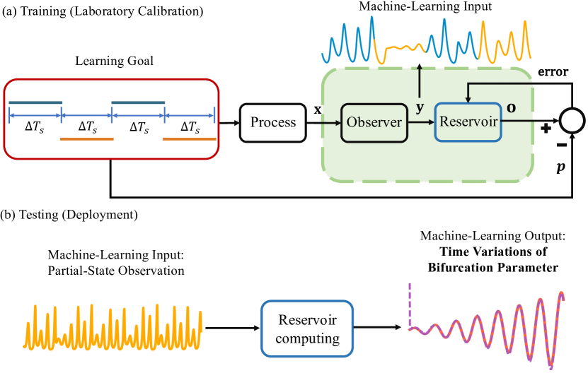
Figure 1: Proposed reservoir-computing based parameter tracking scheme. The goal is to track a parameter of the system from which only partial state observation is available. The output of the reservoir computer is $o(t)$. (a) In the training or laboratory calibration phase, the input to the neural network is an integrated vector time series $\mathbf{y}_{T}(t)$ recombining segments of the time series from partial state observation for a small number of parameter values. The training goal is the corresponding piecewise constant function of the parameter values versus time, denoted as $p(t)$, i.e., minimizing the error between $p(t)$ and $o(t)$. (b) In the testing or deployment phase where the parameters are inaccessible, the input to the neural network is the current observation vector time series $\mathbf{y}(t)$ and the output is the parameter as a function of time.

We consider three prototypical nonlinear dynamical systems: a three-species chaotic food chain system [38], the chaotic Rössler oscillator [39], and the Mackey-Glass delay-differential equation system [40]. The first two systems are three-dimensional while the Mackey-Glass system is non-Markovian with an infinite-dimensional phase space. For each system, three types of parameter variations are considered: frequency modulation (FM), sawtooth wave, and amplitude modulation (AM), with different numbers of parameter sampling in different ranges for training. The machine-learning performance is characterized by the root-mean-square error (RMSE). Here we present the results from the chaotic food-chain system given by (results for the other two systems can be found in SI [9]): $dR/dt=R(1-R/{\rm K})-{\rm x_{c}y_{c}}CR/(R+{\rm R_{0}})$, $dC/dt={\rm x_{c}}C[{\rm y_{c}}R/(R+{\rm R_{0}})-1]-{\rm x_{p}y_{p}}PC/(C+{\rm C_{0}})$, $dP/dt={\rm x_{p}}P[{\rm y_{p}}C/(C+{\rm C_{0}})-1]$, where $R$, $C$, and $P$ are the population densities of the resource, consumer, and predator species, respectively. The system has seven parameters: ${\rm K,x_{c},y_{c},x_{p},y_{p},R_{0},C_{0}}>0$. To illustrate the process of parameter tracking, we assume that the following three parameters: ${\rm K,y_{c},y_{p}}$ are time-varying, and fix all other parameters at constant values: $\rm x_{c}=0.4$, $x_{p}=0.08$, $C_{0}=0.5$, and $R_{0}=0.16129$, according to some bioenergetics argument [38]. We focus on tracking a single parameter: $\rm{K}$, $\rm{y_{c}}$, or $\rm{y_{p}}$, whose respective nominal values are 0.94, 1.7, and 5.0. When tracking one of the three parameters, the other two are fixed at their respective nominal values.

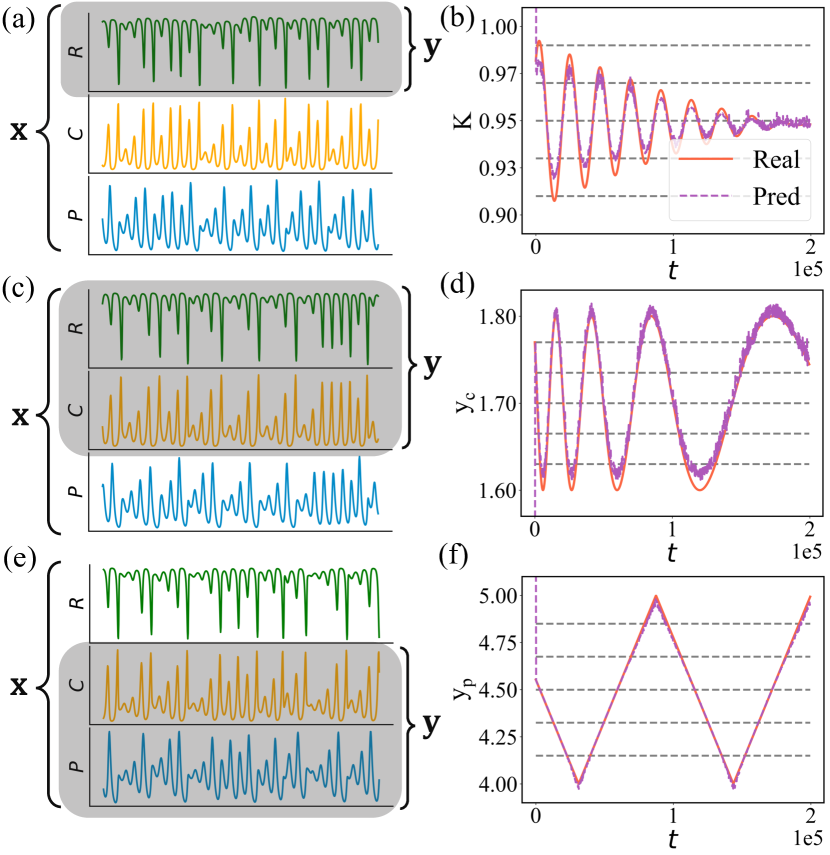
Figure 2: Tracking time-varying parameters of the chaotic food-chain system. Different combinations of the parameter waveforms and partial state observation are illustrated: the top, middle, and bottom row correspond to three types of parameter variations (AM, FM, and sawtooth waveform), while the gray shaded region in the left column illustrates the partial state observation. The right column gives the results of parameter tracking in comparison with the ground truth. (a,b) One-dimensional observational state variable $\mathbf{y}=(R)$ for tracking AM parameter $\rm{K}$; (c,d) Two-dimensional observation $\mathbf{y}=(R,C)$ for tracking FM parameter $\rm{y_{c}}$; (e,f) Two-dimensional observation $\mathbf{y}=(C,P)$ for tracking the sawtooth-wave parameter $\rm{y_{p}}$. The five horizontal dashed lines indicate the parameter values from which training data are generated, i.e., $s_{n}=5$.

Figure 2 exemplifies the results of tracking the three different types of parameter variations for different combinations of the bifurcation parameter and state observation. The computational setting is as follows. Time series are generated by integrating the system model using the time step $dt=0.01$. The initial states of both the dynamical process and the reservoir neural network are randomly chosen from a uniform distribution. The training and testing data are obtained by sampling the time series at the interval $\Delta_{s}$. We set $\Delta_{s}=250dt=2.5$, corresponding to approximately $1/25$ cycles of oscillation in the chaotic food-chain system. Let $\Delta T_{s}$ be the switching time interval in which the target parameter is a constant. The training time is $900\Delta T_{s}$. The testing length is chosen to be slightly longer than the training length, enough for tracking several cycles of the parameter variation. The size of the reservoir network is $D_{r}=500$ and the bias number is set to one. The other six hyperparameters are determined by Bayesian optimization (SI [9]), which are fixed during training and testing. Often, a constant bias may arise between the machine predicted parameter variation and the ground truth, which can be removed by calibrating using two parameter values (SI [9]). The results in Fig. 2 indicate that the machine-learning framework is capable of accurate parameter tracking based on partial state observation only.

Two characteristics of the bifurcation parameter values used in the training which can affect significantly the performance of tracking are the number of such parameter values (denoted as $s_{n}$) and the relative range of the parameter variation (denoted as $s_{w}$) from which the training time series data are generated. Intuitively, if the training data come from only one value of the bifurcation parameter, it will not be possible for the reservoir computer to learn the features of parameter variation, resulting in a large tracking error. As $s_{n}$ increases from one, we expect the error to decrease. What is the minimum number of bifurcation parameter values required for accurate parameter tracking? Likewise, if the bifurcation parameter values are taken from the full range of the actual parameter variation, accurate tracking is likely, resulting in a small error. As the range $s_{w}$ is reduced, the error will increase. How tolerant can the machine-learning parameter tracking scheme be with respect to this range?

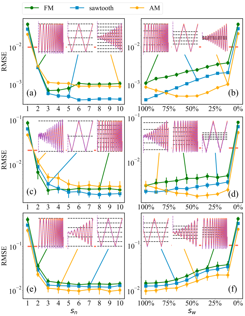
Figure 3: Effects of the training bifurcation-parameter values on tracking. The two relevant quantities are $s_{n}$ - the number of distinct bifurcation-parameter values for training, and $s_{w}$ - the relative parameter range from which time series are taken for training. (a,c,e) Testing RMSE versus $s_{n}$ for parameters $\rm{K}$, $\rm{y_{c}}$, and $\rm{y_{p}}$, respectively. (b,d,f) Testing RMSE versus $s_{w}$ for $\rm{K}$, $\rm{y_{c}}$, and $\rm{y_{p}}$, respectively. Each panel has results from FM, sawtooth, and AM types of parameter variations, and each point is the result of averaging over 50 independent realizations. The results in (a,c,e) indicates that using time series from three distinct values of the bifurcation parameter suffices to guarantee accurate parameter tracking. The results in (b,d,f) suggests acceptable parameter-tracking performance for $s_{w}>20\%$.

Figures 3(a,c,e) demonstrate the effect of varying $s_{n}$ on the parameter-tracking performance for different combinations of the bifurcation parameter and its time variations. It can be seen that, for all cases illustrated, the testing error decreases dramatically as $s_{n}$ increases from one to three, and remains approximately constant afterwards, indicating that using the time series from as few as three values of the bifurcation parameter suffices for accurate tracking of the actual parameter variations. Figures 3(b,d,f) show the effect of varying the relative range $s_{w}$ on the tracking performance. As $s_{w}$ decreases from $100\%$, the RMSE increases, but it does so in a slow manner until $s_{w}$ falls below about $20\%$, indicating that the machine-learning parameter tracking scheme is remarkably tolerant to the range of the bifurcation parameter from which the time series for training are generated.

A key feature of our work is that machine-learning parameter tracking can be done using only partial state observation. But how partial can the observation be while still delivering reasonable parameter tracking performance? For $\mathbf{x}\equiv(x_{1},x_{2},x_{3})^{T}$, full state observation is represented by $\mathbf{y}=\mathbf{x}$. There are six cases of partial state observation: $\mathbf{y}=(x_{1})$, $\mathbf{y}=(x_{2})$, $\mathbf{y}=(x_{3})$, $\mathbf{y}=(x_{1},x_{2})$, $\mathbf{y}=(x_{1},x_{3})$, and $\mathbf{y}=(x_{2},x_{3})$. Altogether, there are seven distinct cases of state observation. For each case, we conduct a reasonable of number (e.g., 50) of tests. For each test, we define an error threshold. If the resulting testing RMSE is below the threshold, the test is deemed successful. The fraction of successful cases gives the success probability. We then calculate, for different types of parameter variations, the success rate $\rm P_{s}$ and use a bar graph to represent the rate for the seven cases of state observation. Some representative results for the chaotic food-chain system are shown in Fig. 4. It can be seen that in most cases, close to $100\%$ success rate can be achieved by observing two state variables. Depending on the specific parameter, in some cases observing even one state variable can lead to satisfactory success rate.

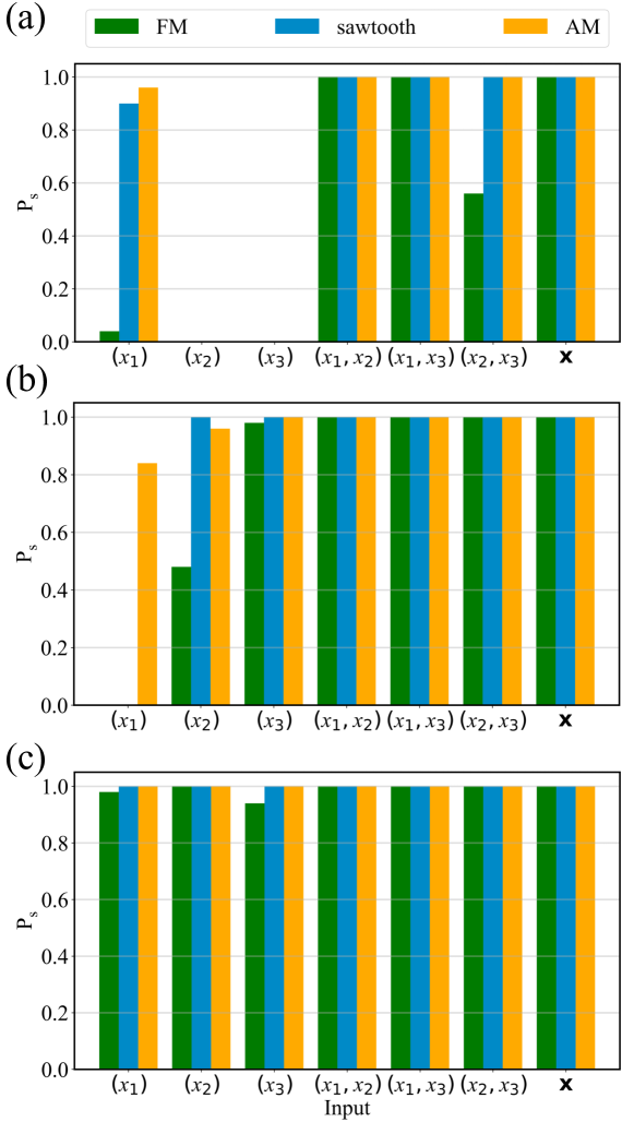
Figure 4: Success probability for different partial observation scenarios for the chaotic food-chain system. (a-c) Bar-graph representation of the success rate for the seven distinct cases of state observation for the three different bifurcation parameters, for three types of parameter variation (FM: green; sawtooth: blue; AM: yellow). The success rate is calculated from 50 independent realizations. In most cases, observing two state variables can lead to nearly $100\%$ success rate.

In summary, we developed a reservoir-computing based framework to continuously track parameter variations with time based on observation from a subset of the full state variables. Relying on partial observation is necessary in real applications where not all the dynamical variables of the system are accessible and there can be unknown hidden variables. Our unique training scheme enables the reservoir computer to learn the correspondence between the input time series and the underlying parameter value so that it is able to forecast the parameter variations with time based in input time series from partial state observation. We demonstrated the working of the proposed parameter-tracking framework using chaotic systems subject to three distinct types of parameter variations. The effects of a number of factors on the tracking performance were investigated: minimally required bifurcation parameter values for training, the number of state vectors associated with partial-state observation, measurement and dynamical noises, network size and training time, and the minimum switching time required of the training data (SI [9]). The developed reservoir-computing based scheme represents a general and robust parameter-tracking framework that can be deployed in real-world applications.

A possible application is in epidemiology. For example, some virus has seasonal behaviors: its spreading rate varies in different seasons. Our framework can be used to track the spreading rate change with time based on state evolution, thereby enabling accurate prediction of the infection scale and period. Another potential application is predicting if a dynamical system is about to approach a tipping point at which a transition from a normal to a collapsing (e.g., large-scale extinction in an ecosystem) steady state occurs. With inevitable noises, we can use the noisy time series from partial state observation as the input to our machine-learning scheme to generate the time-varying behavior of some key bifurcation parameters of the system. Based on the predicted trend of the parameter variation, the chance of a tipping point occurring in the near future can be assessed.

This work was supported by the Air Force Office of Scientific Research through Grant No. FA9550-21-1-0438.

References

- Grebogi et al. [1983] C. Grebogi, E. Ott, and J. A. Yorke, Crises, sudden changes in chaotic attractors and chaotic transients, Physica D 7, 181 (1983).
- Lai and Tél [2011] Y.-C. Lai and T. Tél, Transient Chaos - Complex Dynamics on Finite Time Scales, 1st ed. (Springer, New York, 2011).
- Hannink et al. [2016] J. Hannink, T. Kautz, C. F. Pasluosta, K.-G. Gaßmann, J. Klucken, and B. M. Eskofier, Sensor-based gait parameter extraction with deep convolutional neural networks, IEEE J. Biomed. Health Info. 21, 85 (2016).
- Chen and Zhou [2020] Y. Chen and Y. Zhou, Machine learning based decision making for time varying systems: Parameter estimation and performance optimization, Knowle. Based Sys. 190, 105479 (2020).
- Chen et al. [2020] X. Chen, Y. Tian, T. Zhang, and J. Gao, Differential evolution based manifold gaussian process machine learning for microwave filter’s parameter extraction, IEEE Access 8, 146450 (2020).
- Zhang [2021] Y. Zhang, Neural network algorithm with reinforcement learning for parameters extraction of photovoltaic models, IEEE Trans. Neu. Net. Learning. Sys. 34, 2806 (2021).
- Abdusalomov et al. [2022] A. B. Abdusalomov, F. Safarov, M. Rakhimov, B. Turaev, and T. K. Whangbo, Improved feature parameter extraction from speech signals using machine learning algorithm, Sensors 22, 8122 (2022).
- Kao et al. [2022] M.-Y. Kao, F. Chavez, S. Khandelwal, and C. Hu, Deep learning-based BSIM-CMG parameter extraction for 10-nm FinFET, IEEE Trans. Elec. Dev. 69, 4765 (2022).
- [9] Supplementary Information provides details elaborating the results in the main text. It is helpful but not essential for understanding the main results of the paper. It contains the following materials: (1) a background review of the previous methods on static parameter identification and dynamic parameter tracking, as well as the more recent machine-learning approaches, (2) basics of reservoir computing for parameter tracking, (3) additional results for the chaotic food-chain system treated in the main text, which include the number of state vectors associated with partial-state observation, measurement and dynamical noises, network size and training time, and the minimum switching time required of the training data, (4) comprehensive parameter tracking results with the chaotic Rössler system, and (5) comprehensive parameter tracking results from the Mackey-Glass delay-differential equation system .
- Jaeger [2001] H. Jaeger, The “echo state” approach to analysing and training recurrent neural networks-with an erratum note, Bonn, Germany: German National Research Center for Information Technology GMD Technical Report 148, 13 (2001).
- Maass et al. [2002] W. Maass, T. Natschläger, and H. Markram, Real-time computing without stable states: A new framework for neural computation based on perturbations, Neu. Comp. 14, 2531 (2002).
- Lukoševičius and Jaeger [2009] M. Lukoševičius and H. Jaeger, Reservoir computing approaches to recurrent neural network training, Compu. Sci. Rev. 3, 127 (2009).
- Appeltant et al. [2011] L. Appeltant, M. C. Soriano, G. Van der Sande, J. Danckaert, S. Massar, J. Dambre, B. Schrauwen, C. R. Mirasso, and I. Fischer, Information processing using a single dynamical node as complex system, Nat. Commun. 2, 1 (2011).
- Haynes et al. [2015] N. D. Haynes, M. C. Soriano, D. P. Rosin, I. Fischer, and D. J. Gauthier, Reservoir computing with a single time-delay autonomous Boolean node, Phys. Rev. E 91, 020801 (2015).
- Larger et al. [2017] L. Larger, A. Baylón-Fuentes, R. Martinenghi, V. S. Udaltsov, Y. K. Chembo, and M. Jacquot, High-speed photonic reservoir computing using a time-delay-based architecture: Million words per second classification, Phys. Rev. X 7, 011015 (2017).
- Pathak et al. [2017] J. Pathak, Z. Lu, B. Hunt, M. Girvan, and E. Ott, Using machine learning to replicate chaotic attractors and calculate Lyapunov exponents from data, Chaos 27, 121102 (2017).
- Lu et al. [2017] Z. Lu, J. Pathak, B. Hunt, M. Girvan, R. Brockett, and E. Ott, Reservoir observers: Model-free inference of unmeasured variables in chaotic systems, Chaos 27, 041102 (2017).
- Pathak et al. [2018] J. Pathak, B. Hunt, M. Girvan, Z. Lu, and E. Ott, Model-free prediction of large spatiotemporally chaotic systems from data: A reservoir computing approach, Phys. Rev. Lett. 120, 024102 (2018).
- Carroll [2018] T. L. Carroll, Using reservoir computers to distinguish chaotic signals, Phys. Rev. E 98, 052209 (2018).
- Nakai and Saiki [2018] K. Nakai and Y. Saiki, Machine-learning inference of fluid variables from data using reservoir computing, Phys. Rev. E 98, 023111 (2018).
- Roland and Parlitz [2018] Z. S. Roland and U. Parlitz, Observing spatio-temporal dynamics of excitable media using reservoir computing, Chaos 28, 043118 (2018).
- Griffith et al. [2019] A. Griffith, A. Pomerance, and D. J. Gauthier, Forecasting chaotic systems with very low connectivity reservoir computers, Chaos 29, 123108 (2019).
- Jiang and Lai [2019] J. Jiang and Y.-C. Lai, Model-free prediction of spatiotemporal dynamical systems with recurrent neural networks: Role of network spectral radius, Phys. Rev. Res. 1, 033056 (2019).
- Tanaka et al. [2019] G. Tanaka, T. Yamane, J. B. Héroux, R. Nakane, N. Kanazawa, S. Takeda, H. Numata, D. Nakano, and A. Hirose, Recent advances in physical reservoir computing: A review, Neu. Net. 115, 100 (2019).
- Fan et al. [2020] H. Fan, J. Jiang, C. Zhang, X. Wang, and Y.-C. Lai, Long-term prediction of chaotic systems with machine learning, Phys. Rev. Res. 2, 012080 (2020).
- Zhang et al. [2020] C. Zhang, J. Jiang, S.-X. Qu, and Y.-C. Lai, Predicting phase and sensing phase coherence in chaotic systems with machine learning, Chaos 30, 083114 (2020).
- Klos et al. [2020] C. Klos, Y. F. K. Kossio, S. Goedeke, A. Gilra, and R.-M. Memmesheimer, Dynamical learning of dynamics, Phys. Rev. Lett. 125, 088103 (2020).
- Kong et al. [2021a] L.-W. Kong, H.-W. Fan, C. Grebogi, and Y.-C. Lai, Machine learning prediction of critical transition and system collapse, Phys. Rev. Res. 3, 013090 (2021a).
- Patel et al. [2021] D. Patel, D. Canaday, M. Girvan, A. Pomerance, and E. Ott, Using machine learning to predict statistical properties of non-stationary dynamical processes: System climate, regime transitions, and the effect of stochasticity, Chaos 31, 033149 (2021).
- Kim et al. [2021] J. Z. Kim, Z. Lu, E. Nozari, G. J. Pappas, and D. S. Bassett, Teaching recurrent neural networks to infer global temporal structure from local examples, Nat. Machine Intell. 3, 316 (2021).
- Fan et al. [2021] H. Fan, L.-W. Kong, Y.-C. Lai, and X. Wang, Anticipating synchronization with machine learning, Phys. Rev. Res. 3, 023237 (2021).
- Kong et al. [2021b] L.-W. Kong, H.-W. Fan, C. Grebogi, and Y.-C. Lai, Emergence of transient chaos and intermittency in machine learning, J. Phys. Complex. 2, 035014 (2021b).
- Bollt [2021] E. Bollt, On explaining the surprising success of reservoir computing forecaster of chaos? The universal machine learning dynamical system with contrast to VAR and DMD, Chaos 31, 013108 (2021).
- Gauthier et al. [2021] D. J. Gauthier, E. Bollt, A. Griffith, and W. A. Barbosa, Next generation reservoir computing, Nat. Commun. 12, 1 (2021).
- Carroll [2022] T. L. Carroll, Optimizing memory in reservoir computers, Chaos 32, 023123 (2022).
- Kong et al. [2023] L.-W. Kong, Y. Weng, B. Glaz, M. Haile, and Y.-C. Lai, Reservoir computing as digital twins for nonlinear dynamical systems, Chaos 33, 033111 (2023).
- Kim and Bassett [2023] J. Z. Kim and D. S. Bassett, A neural machine code and programming framework for the reservoir computer, Nat. Mach. Intell. 5, 622 (2023).
- McCann and Yodzis [1994] K. McCann and P. Yodzis, Nonlinear dynamics and population disappearances, Ame. Natural. 144, 873 (1994).
- Rössler [1976] O. E. Rössler, An equation for continuous chaos, Phys. Lett. A 57, 397 (1976).
- Mackey and Glass [1977] M. C. Mackey and L. Glass, Oscillation and chaos in physiological control systems, Science 197, 287 (1977).