Rate-induced tipping in complex high-dimensional ecological networks

Abstract

In an ecosystem, environmental changes as a result of natural and human processes can cause some key parameters of the system to change with time. Depending on how fast such a parameter changes, a tipping point can occur. Existing works on rate-induced tipping, or R-tipping, offered a theoretical way to study this phenomenon but from a local dynamical point of view, revealing, e.g., the existence of a critical rate for some specific initial condition above which a tipping point will occur. As ecosystems are subject to constant disturbances and can drift away from their equilibrium point, it is necessary to study R-tipping from a global perspective in terms of the initial conditions in the entire relevant phase space region. In particular, we introduce the notion of the probability of R-tipping defined for initial conditions taken from the whole relevant phase space. Using a number of real-world, complex mutualistic networks as a paradigm, we discover a scaling law between this probability and the rate of parameter change and provide a geometric theory to explain the law. The real-world implication is that even a slow parameter change can lead to a system collapse with catastrophic consequences. In fact, to mitigate the environmental changes by merely slowing down the parameter drift may not always be effective: only when the rate of parameter change is reduced to practically zero would the tipping be avoided. Our global dynamics approach offers a more complete and physically meaningful way to understand the important phenomenon of R-tipping.

This manuscript was compiled on

In complex dynamical systems, the phenomenon of tipping point, characterized by an abrupt transition from one type of behavior (typically normal, healthy, or survival) to another type (e.g., catastrophic), has received growing attention (1, 2, 3, 4, 5, 6, 7, 8, 9, 10, 11, 12, 13, 14, 15, 16, 17, 18, 19, 20, 21, 22, 23, 24, 25). A tipping point is often of significant concern because it is a point of “no return” in the parameter space, manifested by the collapse of the system as a parameter passes through a critical value. In ecological systems, sudden extinction of species on a large scale can be the result of a tipping point (1, 2, 3, 4). Tipping points can arise in diverse contexts such as the outbreak of epidemics (26), global climate changes (27), and the sudden transition from normal to depressed mood in bipolar patients (28). In nonlinear dynamics, a common type of bifurcation responsible for a tipping point is saddle-node bifurcations (forward or backward). Consider the situation where, in the parameter regime of interest, there are two coexisting stable steady states: a “high” state corresponding to normal or “survival” functioning and a “low” or “extinction” state, each with its own basin of attractor. Suppose external factors such as climate change cause a bifurcation parameter of the system to increase. A tipping point is a backward saddle-node bifurcation, after which the “survival” fixed point disappears, leaving the “extinction” state as the only destination of the system, where the original basin of the “survival” state is absorbed into the basin of the “extinction” state.

In real-world dynamical systems, parameters are not stationary but constantly drift in time. A known example is the slow increase in the average global temperature with time due to human activities. In ecological systems, some key parameters such as the carrying capacity or the species decay rate can change with time, and there is a global tendency for such parameter changes to “speed up.” In fact, the rate of environmental change is an important driver across different scales in ecology (29). The behavior of the parameter variations with time introduces another “meta” parameter into the dynamical process: the rate of change of the parameters. About ten years ago, it was found that the rate can induce a tipping point - the phenomenon of rate-induced tipping or R-tipping (9), which is relevant to fields such as climate science (30, 31), neuroscience (32, 33), vibration engineering (34), and even competitive economy (35). Existing studies of R-tipping were for low-dimensional dynamical systems and the analysis approaches were “local” in the sense that they focused on the behaviors of some specific initial condition and trajectory, addressing issues such as the critical rate for tipping (36, 37). In particular, with respect to a specific initial condition, R-tipping in these studies was defined as an abrupt change in the behavior of the system (or a critical transition) taking place at a specific rate of change of a bifurcation parameter (9).

The state that an ecological system is in depends on a combination of deterministic dynamics, small scale stochastic influences (e.g., demographic stochasticity (38)), and large stochastic disturbances such as drought or other significant climatic event (39). So when considering future dynamics of ecological systems it makes sense to consider systems that may be far from equilibrium, but still within the basin of attraction of an equilibrium, rather than starting at the equilibrium. High-dimensional ecological systems are particularly likely to be found far from equilibrium. In fact, it has been suggested that it can be common for ecosystems to be in some transient state (40, 41).

In this paper, we focus on high-dimensional, empirical ecological networks and investigate R-tipping with two key time-varying parameters by presenting a computationally feasible, “global” approach to exploring the entire relevant phase space region with analytic insights. We focus on a representative class of such systems: mutualistic networks (42, 43, 44, 14, 45, 46, 47, 17, 21, 19, 48) that are fundamental to ecological systems, which are formed through mutually beneficial interactions between two groups of species. In a mutualistic network, a species in one group derives some form of benefit from the relationship with some species in the other group. Examples include the corals and the single-celled zooxanthellae that form the large-scale coral reefs, and the various networks of pollinators and plants in different geographical regions of the world. These networks influence biodiversity, ecosystem stability, nutrient cycling, community resilience, and evolutionary dynamics (49), and they are a key aspect of ecosystem functioning with implications for conservation and ecosystem management. Understanding the ecological significance of mutualistic networks is crucial for unraveling the complexities of ecological communities and for implementing effective strategies to safeguard biodiversity and ecosystem health (50). Mathematically, because of the typically large number of species involved in the mutualistic interactions, the underlying networked systems are high-dimensional nonlinear dynamical systems.

We first ask if R-tipping can arise in such high-dimensional systems through simulating a number of empirical pollinator-plant mutualistic networks (see Tab. 1) and obtain an affirmative answer. Our computations reveal that the critical rate above which a tipping point occurs depends strongly on the initial condition. Rather than studying the critical rate for any specific initial condition, we go beyond the existing local analysis approaches by investigating the probability of R-tipping for a large ensemble of initial conditions taken from the whole relevant phase space and asking how this probability, denoted as $\Phi(r)$, depends on the rate $r$ of parameter change. We discover a scaling law between $\Phi(r)$ and $r$: as the rate increases, the probability first increases rapidly, then slowly, and finally saturates. Using a universal two-dimensional (2D) effective model that was validated to be particularly suitable for predicting and analyzing tipping points in high-dimensional mutualistic networks (17), we analytically derive the scaling law. Specifically, let $\kappa(t)$ be the parameter that changes with time linearly at the rate $r$ in a finite range, denoted as $[\kappa_{\rm min},\kappa_{\rm max}]$. The scaling law is given by

$$\Phi(r)\sim\exp{[-C(\kappa_{\rm max}-\kappa_{\rm min})/r]},$$ (1)

where $C>0$ is a constant. Our theoretical analysis indicates that, for 2D systems, $C$ is nothing but the maximum possible unstable eigenvalue of the mediating unstable fixed point on the boundary separating the basins of the survival and extinction attractors when the parameter $\kappa$ varies in the range $[\kappa_{\rm min},\kappa_{\rm max}]$. However, for high-dimensional systems, such correspondence does not hold, but $C$ can be determined through a numerical fitting.

The scaling law (1) has the following features. First, the probability $\Phi(r)$ is an increasing function of $r$ for $r>0$ [$\Phi^{\prime}(r)>0$]. Second, $\Phi^{\prime}(r)$ is a decreasing function of $r$, i.e., the increase of $\Phi(r)$ with $r$ slows down with $r$ and the rate of increase becomes zero for $r\rightarrow\infty$. Third, the rate of increase in $\Phi(r)$ with $r$ is the maximum for $r\gtrsim 0$, and $\Phi(r)$ becomes approximately constant for $r>r^{*}\sim\sqrt{(\kappa_{\rm max}-\kappa_{\rm min})}$. This third feature has a striking implication because the probability of R-tipping will grow dramatically as soon as the rate of parameter change increases from zero. The real-world implication is alarming because it means that even a slow parameter change can lead to a system collapse with catastrophic consequences. To control or mitigate the environmental changes by merely slowing down the parameter drift may not always be effective: only when the rate of parameter change is reduced to practically zero would the tipping be avoided!

Alternatively, the scaling law (1) can be expressed as the following explicit formula:

$$\Phi(r)=B\exp{[-C(\kappa_{\rm max}-\kappa_{\rm min})/r]}$$ (2)

with an additional positive constant $B$. For 2D systems, $B$ is the difference between the basin areas of the extinction state for $\kappa=\kappa_{\rm max}$ and $\kappa=\kappa_{\rm min}$. For high-dimensional systems, $B$ can be determined numerically.

While a comprehensive understanding of the entire parameter space as well as the rates and directions of change associated with these parameters are worth investigating, the picture that motivated our work was the potential impacts of ongoing climate change on ecological systems. Under climate change, various parameters can vary in different directions, and some changes might offset the effects of others. Our focus is on the scenarios where the changes in parameters align with the observed detrimental environmental impacts. For example, consistent with environmental deterioration, in a mutualistic network the species decay rate can increase, and/or the mutualistic interaction strength can decrease. A simultaneous increase in the species decay rate and mutualistic strength does not seem physically reasonable in this context. We thus study scenarios of multiple parameter variations that align with the realistic climate change impacts by carrying out computations with a systematic analysis of the tipping-point transitions in the two-dimensional parameter plane of the species decay rate and the mutualistic interaction strength.

Results

We consider the empirical mutualistic pollinator–plant networks from the Web of Life database (www.Web-of-Life.es). The needs to search for the parameter regions exhibiting R-tipping and to simulate a large number of initial conditions in the phase space as required by our global analysis approach, as well as the high dimensionality of the empirical mutualistic networks demand extremely intensive computation (51). To make the computation feasible, we select ten networks to represent a diverse range of mutualistic interactions from different regions of the world and highlight the generality of our approach to R-tipping and the scaling law. The basic information about these networks such as the name of the networks, the countries where the empirical data were collected, and the number of species in each network, is listed in Tab. 1. The dynamics of a mutualistic network of $N_{A}$ pollinator and $N_{P}$ plant species, taking into account the generic plant-pollinator interactions (42), can be described by a total of $N=N_{A}+N_{P}$ nonlinear differential equations of the Holling type (52) in terms of the species abundances as

$$\dot{P}_{i}= P_{i}\Big{(}\alpha_{i}^{P}-\sum_{l=1}^{N_{p}}\beta_{il}^{P}P_{l}+\frac{\sum_{j=1}^{N_{A}}\gamma_{ij}^{P}A_{j}}{1+h\sum_{j=1}^{N_{A}}\gamma_{ij}^{P}A_{j}}\Big{)},$$ (3a)

$$\dot{A}_{j}= A_{j}\Big{(}\alpha_{j}^{A}-\kappa_{j}-\sum_{l=1}^{N_{A}}\beta_{jl}^{A}A_{l}+\frac{\sum_{i=1}^{N_{P}}\gamma_{ji}^{A}P_{i}}{1+h\sum_{i=1}^{N_{P}}\gamma_{ji}^{A}P_{i}}\Big{)},$$ (3b)

where $P_{i}$ and $A_{j}$ are the abundances of the $i^{th}$ and $j^{th}$ plant and pollinator species, respectively, $i=1,\ldots,N_{P}$, $j=1,\ldots,N_{A}$, $\kappa$ is the pollinator decay rate, $\alpha^{P(A)}$ is the intrinsic growth rate in the absence of intraspecific competition and any mutualistic effect, $h$ is the half-saturation constant. Intraspecific and interspecific competition of the plants (pollinators) is characterized by the parameters $\beta_{ii}^{P}$ ($\beta_{jj}^{A}$) and $\beta_{il}^{P}$ ($\beta_{jl}^{A}$), respectively. The mutualistic interactions as characterized by the parameter $\gamma_{ij}^{P}$ can be written as $\gamma_{ij}^{P}=\xi_{ij}\gamma_{0}/K_{i}^{\tau}$, where $\xi_{ij}=1$ if there is a mutualistic interaction between the $i^{th}$ plant and $j^{th}$ pollinator (zero otherwise), $\gamma_{0}$ is a general interaction parameter, $K_{i}$ is the degree of the $i^{th}$ plant species in the network, and $\tau$ determines the strength of the trade-off between the interaction strength and the number of interactions. (The expression for $\gamma_{ji}^{A}$ is similar.)

Table 1: Empirical mutualistic networks studied in this work and their corresponding range of parameter change and fitting constants in Eq. (1)

Network	Country	$N_{P}$	$N_{A}$	$\kappa$-interval	$B$	$C$
M_PL_008	Canary Islands	$11$	$38$	${[0.90,0.93]}$	$0.36$	$0.19$
M_PL_013	South Africa	$9$	$56$	${[0.70,0.99]}$	$0.07$	$0.11$
M_PL_022	Argentina	$21$	$45$	${[0.75,0.93]}$	$0.88$	$0.12$
M_PL_023	Argentina	$23$	$72$	$[0.87,0.96]$	$0.59$	$0.09$
M_PL_027	New Zealand	$18$	$60$	$[0.90,0.95]$	$0.49$	$0.09$
M_PL_032	USA	$7$	$33$	$[0.82,0.99]$	$0.55$	$0.19$
M_PL_036	Açores	$10$	$12$	$[0.74,0.88]$	$0.39$	$0.12$
M_PL_037	Denmark	$10$	$40$	$[0.87,0.93]$	$0.23$	$0.15$
M_PL_038	Denmark	$8$	$42$	$[0.85,0.95]$	$0.30$	$0.15$
M_PL_045	Greenland	$17$	$26$	$[0.96,0.98]$	$0.09$	$0.05$

The computational setting of our study is as follows. In the network system described by Eqs. 3a and 3b, the number of the equations determines the phase-space dimension of the underlying nonlinear dynamical system. There are a large number of basic parameters in the model, such as $\gamma$ that quantifies the strength of the mutualistic interactions and $\kappa$ characterizing the species decay rate. In the context of R-tipping, while all the parameters should be time-varying in principle, to make our study computationally feasible, we assume that the two key parameters ($\kappa$ and $\gamma$) are time-dependent while keeping the other parameters fixed. Since the defining characteristic of a system exhibiting a tipping point is the coexistence of two stable steady states: survival and extinction, we focus on the range of parameter variations in which the network system under study exhibits the two stable equilibria. When presenting our results (Fig. 1 below and Figs. S4-S14 in Supplementary Information), in each case the parameter variation is along a specific direction in the two-dimensional parameter plane: $\kappa$ and $\gamma$ with the goal to understand how changes in these two parameters impact the R-tipping probability.

To introduce the rate change of a parameter, we consider the scenario where negative environmental impacts cause the species decay rate to increase linearly with time at the rate $r$ from a minimal value $\kappa_{\rm min}$ to a maximal value $\kappa_{\rm max}$:

$$\dot{\kappa}_{j}=\begin{cases}r\quad{\rm if}\quad\kappa_{\rm min}<\kappa_{j}<\kappa_{\rm max}\\ 0\quad\quad{\rm otherwise.}\end{cases}$$ (4)

(For mutualistic networks, another relevant parameter that is vulnerable to environmental change is the mutualistic interaction strength. The pertinent results are presented in Supplementary Information.) To calculate the probability of R-tipping, $\Phi(r)$, we set $r=0$ so that $\kappa=\kappa_{\rm min}$, solve Eqs. (3a) and (3b) numerically for a large number of random initial conditions chosen uniformly from the whole high-dimensional phase space, and determine $10^{5}$ initial conditions that approach the high stable steady state in which no species becomes extinct. We then increase the rate $r$ from zero. For each fixed value of $r$, we calculate, for each of the selected $10^{5}$ initial conditions, whether or not the final state is the high stable state. If yes, then there is no R-tipping for the particular initial condition. However, if the final state becomes the extinction state, R-tipping has occurred for this value of $r$. The probability $\Phi(r)$ can be approximated by the fraction of the number of initial conditions leading to R-tipping out of the $10^{5}$ initial conditions.

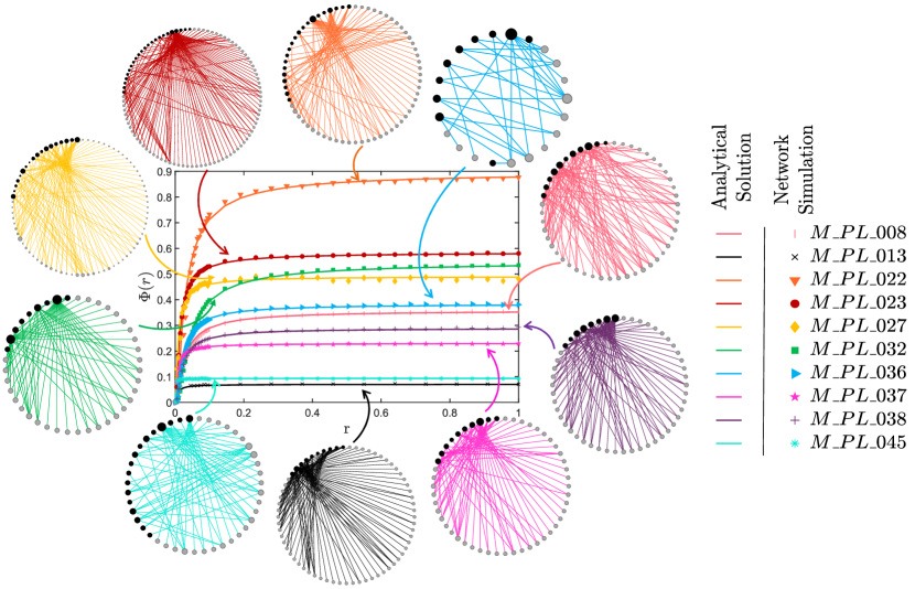
Figure 1: Probability $\Phi(r)$ of R-tipping versus the time rate $r$ of parameter change for ten real-world mutualistic networks, together with the corresponding bipartite structure for each network. The dots are the probability calculated by simulating Eqs. (3a), (3b), and (4), with an ensemble of random initial conditions. The solid curves are the analytic results from Eq. (1), with the two fitting parameters $B$ and $C$ given in Tab. 1. Other parameter values are $\alpha=0.3$, $\beta=1$, $h=0.4$, $\gamma^{P}=1.93$, and $\gamma^{A}=1.77$.

Figure 1 shows $\Phi(r)$ versus $r$ for the ten empirical mutualistic networks specified in Tab. 1, together with the bipartite network structure, which are distinguished by different colors. For each network, the interval $[\kappa_{\rm min},\kappa_{\rm max}]$ of the bifurcation parameter (listed in the fifth column of Tab. 1) is chosen such that the dynamical network for static parameter values exhibits two stable steady states and a tipping point in this interval, as determined by a computational bifurcation analysis of the species abundances versus $\kappa$. Despite the differences in the topology and the specific parameter values among the empirical networks, it is remarkable that the probability of R-tipping exhibits a characteristic behavior common among all the networks: as the time-varying rate of the bifurcation parameter increases from zero, the probability increases rapidly and then saturates at an approximately finite constant value, as quantified by the analytic scaling law (1). The final or asymptotic value of the R-tipping probability attained in the regime of large time rate of change of the bifurcation parameter depends on the specifics of the underlying mutualistic network in terms of its topological structure and basic system parameters. For example, the total number of species, or the phase-space dimension of the underlying dynamical system, and the relative numbers of the pollinator and plant species vary dramatically across the ten networks, as indicated by the ten surrounding network-structure diagrams in Fig. 1. The structural and parametric disparities among the networks lead to different relative basin volumes of the survival and extinction stable steady states, giving rise to distinct asymptotic probabilities of R-tipping.

The ecological interpretation of the observed different asymptotic values of the R-tipping probability is, as follows. Previous studies revealed the complex interplay between the structural properties of the network and environmental factors in shaping extinction probabilities (53, 54, 55, 56, 57, 58, 59, 60). For example, it was discovered (53) that the plant species tend to play a more significant role in the health of the network system as compared to pollinators (53) in the sense that plant extinction due to climate change is more likely to trigger pollinator coextinction than the other way around. In another example, distinct topological features were found to be associated with the networks with a higher probability of extinction (54, 55). It was also found that robust plant-pollinator mutualistic networks tend to exhibit a combination of compartmentalized and nested patterns (55). More generally, mutualistic networks in the real world are quite diverse in their structure and parameters, each possessing one or two or all the features including lower interaction density, heightened specialization, fewer pollinator visitors per plant species, lower nestedness, and lower modularity, etc. (54, 55, 56, 57, 58, 59, 60). It is thus reasonable to hypothesize that the asymptotic value of the R-tipping probability can be attributed to the sensitivity of the underlying network to environmental changes. For example, a higher (lower) saturation value of the extinction probability can be associated with the networks with a large (small) number of plants and lower (higher) nestedness, network $M\_PL\_22$ (network $M\_PL\_13$). In other examples, network $M\_PL\_32$ can be categorized as “vulnerable” due to its low modularity, despite having a small number of plants, and network $M\_PL\_45$ is resilient against extinction due to its high nestedness and high modularity.

The remarkable phenomenon is that, in spite of these differences, the rapid initial increase in the R-tipping probability is shared by all ten networks! That is when a parameter begins to change with time from zero, even slowly, the probability of R-tipping increases dramatically. The practical implication is that ecosystems with time-dependent parameter drift are highly susceptible to R-tipping. Parameter drifting, even at a slow pace, will be detrimental. This poses a daunting challenge to preserving ecosystems against negative environmental changes. In particular, according to conventional wisdom, ecosystems can be effectively protected by slowing down the environmental changes, but our results suggest that catastrophic tipping can occur with a finite probability unless the rate of the environmental changes is reduced to a near zero value.

To further explore the effects of parameter changes, we study a scenario in which negative environmental impacts cause the species decay rate ($\kappa$) and the mutualistic interaction strength ($\gamma_{0}$) to linearly increase and decrease, respectively. By considering the rate of changing of $\kappa$ ($\gamma_{0}$) as $r_{\kappa}$ ($r_{\gamma_{0}}$), we set $r_{\kappa}=\mathcal{C}r_{\gamma_{0}}$, which allows us to investigate three different scenarios by varying the parameter $\mathcal{C}$: $\mathcal{C}<1$, $\mathcal{C}=1$, and $\mathcal{C}>1$. Figure 2 shows a systematic analysis of the tipping-point transitions in the 2D parameter plane along with the probability of R-tipping for the three different scenarios for the network ${\rm M}\_{\rm PL}\_032$. (The pertinent results for the other nine networks are presented in Sec. 4 in Supporting Information.)

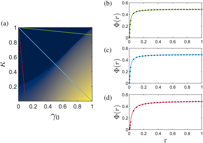
Figure 2: Scaling law of probability of R-tipping in two-dimensional parameter space. (a) Two-dimensional parameter plane of the species decay rate ($\kappa$) and the mutualistic interaction strength ($\gamma_{0}$) for the network ${\rm M}\_{\rm PL}\_032$. The solid lines correspond to the three different scenarios of the parameter $\mathcal{C}$ in calculating the probability of the R-tipping point from $10^{7}$ initial conditions for (b) $\mathcal{C}<1$, (c) $\mathcal{C}=1$, and (d) $\mathcal{C}>1$. Other parameters are $t=0.5$, $\beta=1$, $\alpha=0.3$, $\mu=0$, and $h=0.4$.

To understand the behavior of the R-tipping probability in Fig. 1, we resort to the approach of dimension reduction (61). In particular, for tipping-point dynamics, a high-dimensional mutualistic network can be approximated by an effective model of two dynamical variables: the respective mean abundances of all pollinator and plant species. The effective 2D model can be written as (17)

$$\dot{P} =P\Big{(}\alpha-\beta P+\frac{\gamma^{P}A}{1+h\gamma^{P}A}\Big{)},$$ (5a)

$$\dot{A} =A\Big{(}\alpha-\kappa-\beta A+\frac{\gamma^{A}P}{1+h\gamma^{A}P}\Big{)},$$ (5b)

where $P$ and $A$ are the average abundances of all the plants and pollinators, respectively, $\alpha$ is the effective growth rate and parameter $\beta$ characterizes the combined effects of intraspecific and interspecific competition. The parameters $\gamma^{P}$ and $\gamma^{A}$ are the effective mutualistic interaction strengths that can be determined by the method of eigenvector weighting (17) (Supplementary Note 1). Equations (5a) and (5b) possess five possible equilibria: $\mathbf{f}_{1}\equiv(0,0)^{T}$, $\mathbf{f}_{2}\equiv(\alpha/\beta,0)^{T}$, $\mathbf{f}_{3}\equiv(0,(\alpha-\kappa)/\beta)^{T}$, and $\mathbf{f}_{4,5}\equiv(g_{1},g_{2})^{T}$, where $g_{1}$ and $g_{2}$ are two possible equilibria that depend on the values of the parameters of the model and can be calculated by setting zero the factor in the parentheses of Eqs. (5a) and (5b).

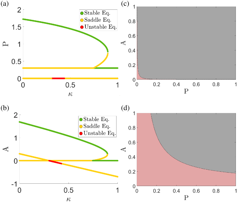
Figure 3: Dynamics of the 2D reduced model Eqs. (5a) and (5b). (a,b) A tipping point occurs as the species decay rate $\kappa$ increases towards one, for the mean plant and pollinator abundances, respectively. The green and yellow curves correspond to the stable and unstable steady states, respectively, where the yellow curve with a red segment is the unstable fixed point $\mathbf{f}_{5}$. The region of bistability is indicated by the blue dot-dashed ellipses. (c,d) Examples of basins of attraction of the 2D model whose parameters are determined as the corresponding averages from the empirical network ${\rm M}\_{\rm PL}\_036$ in Tab. 1 for $\kappa_{min}=0.74$ and $\kappa_{max}=0.88$, respectively. Other parameters are $\alpha=0.3$, $\beta=1$, $h=0.4$, $\gamma^{P}=1.93$, and $\gamma^{A}=1.77$. The pink and gray regions correspond to the basins of the stable steady states $f_{2}$ (extinction) and $f_{4}$ (survival), respectively.

The first equilibrium $\mathbf{f}_{1}$, an extinction state, is at the origin $(P^{*},\,A^{*})=(0,0)$ and is unstable. The second equilibrium $\mathbf{f}_{2}$ is located at the $(P^{*},\,A^{*})=(\alpha/\beta,0)$ and it can be stable or unstable depending on the parameters $\kappa$. The locations of the remaining equilibria depend on the value of $\kappa$. In particular, the third equilibrium $\mathbf{f}_{3}$ can be unstable or nonexistent and the fourth equilibrium $\mathbf{f}_{4}$ is stable and coexists with stable equilibrium $\mathbf{f}_{2}$ in some interval of $\kappa$. The fifth equilibrium $\mathbf{f}_{5}$ is an unstable saddle fixed point in some relevant interval of $\kappa$. Figures 3(a) and 3(b) exemplify the behaviors of the equilibria as $\kappa$ increases from zero to one for $\alpha=0.3$, $\beta=1$, $h=0.4$, $\gamma^{P}=1.93$, and $\gamma^{A}=1.77$, for the average plant and pollinator abundances, respectively. In each panel, the upper green curve is the survival fixed point $\mathbf{f}_{4}$, while the lower horizontal green line corresponds to the extinction state $\mathbf{f}_{2}$. The blue dot-dashed ellipse indicates the interval of $\kappa$ in which two stable equilibria coexist (bistability), whose right edge marks a tipping point.

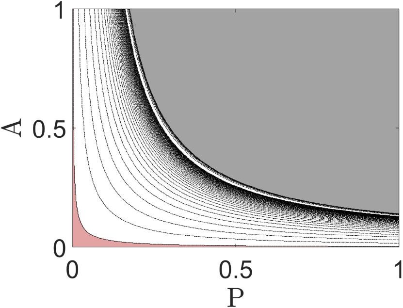
Figure 4: Basin boundary between the extinction and survival fixed-point attractors for different rate of parameter change. Shown are a series of basin boundaries for $r\in[0\,1]$. As $r$ increases from zero, the boundary moves in the direction of large species abundances. The basin boundaries are calculated from the 2D model of the empirical network ${\rm M}\_{\rm PL}\_036$ in Tab. 1. Other parameters are the same as those in Figs. 3(c) and 3(d).

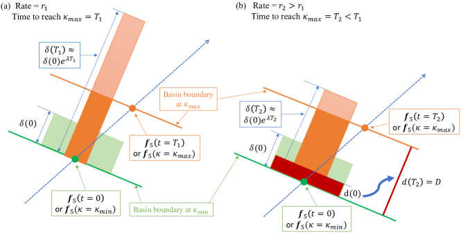
Figure 5: Analysis of the dynamical mechanism responsible for R-tipping. The dynamics of the unstable fixed point $\mathbf{f}_{5}$ together with those of a rectangle region of the initial conditions in its neighborhood are illustrated for two values of the rate of parameter change: (a) $r=r_{1}$ and (b) $r=r_{2}>r_{1}$. At $t=0$ ($\kappa=\kappa_{\rm min}$, a segment of the basin boundary in the vicinity of $\mathbf{f}_{5}$ is illustrated as the solid green line. As the rate of parameter change begins to increase, the basin boundary moves upward and eventually accumulates at that for $\kappa=\kappa_{\rm max}$ - the solid orange lines. For a small rate, the time required for the green boundary to reach the orange boundary is longer. All the initial conditions in the light green region above the green boundary belong to the basin of the survival attractor for $\kappa=\kappa_{\rm min}$, whose trajectories are determined by the local exponentially contracting and expanding dynamics of $\mathbf{f}_{5}$. The fate of these initial conditions is the result of a “race” to go above the orange basin boundary within the “allowed” time duration [$T_{1}$ in (a) and $T_{2}<T_{1}$ in (b)]: those managing to go above will approach the survival attractor, but those that stay below will lead to extinction. Since $T_{1}>T_{2}$, the fraction of initial conditions that can go above in (a) is larger than that in (b), leading to a higher probability of R-tipping for case (b). The precise fraction of those initial conditions is indicated by the red rectangular region in (b), whose initial height stretches to the distance between the green and orange boundaries in the permissible time. This gives the probability of R-tipping as quantified by the scaling law (1). See text for more details.

What will happen to the dynamics when the parameter $\kappa$ becomes time dependent? Without loss of generality, we focus on the interval of $\kappa$ as exemplified by the horizontal range of the dot-dashed ellipse in Figs. 3(a) and 3(b), defined as $[\kappa_{\rm min},\kappa_{\rm max}]$, in which there is bistability in the original high-dimensional network and in the 2D reduced model as well. Note that, for different high-dimensional empirical networks, the values of $\kappa_{\rm min}$ and $\kappa_{\rm max}$ in the 2D effective models are different, as illustrated in the fifth column of Tab. 1. Because of the coexistence of two stable fixed points, for every parameter value in the range $[\kappa_{\rm min},\kappa_{\rm max}]$, there are two basins of attraction, as illustrated in Figs. 3(c) and 3(d) for the 2D effective model of an empirical network ${\rm M}\_{\rm PL}\_036$ for $\kappa=0.74$ and $\kappa=0.88$, respectively, where the pink and gray regions correspond to the basins of the extinction and survival attractors, respectively. The basin boundary is the stable manifold of the unstable fixed point $\mathbf{f}_{5}$. It can be seen that, as $\kappa$ increases, the basin of the extinction attractor increases, accompanied by a simultaneous decrease in the basin area of the survival attractor. This can be understood by comparing the positions of the equilibria in Fig. 3 where, as $\kappa$ increases, the position of survival fixed point $\mathbf{f}_{4}$ moves towards lower plant and pollinator abundances, but the unstable fixed point $\mathbf{f}_{5}$ moves in the opposite direction: the direction of larger species abundances.

The boundary separating the basins of the extinction and survival fixed-point attractors is the stable manifold of $\mathbf{f}_{5}$. As $r$ increases from zero, $\mathbf{f}_{5}$ moves in the direction of larger plant and pollinator abundances, so must the basin boundary, as exemplified in Fig. 4 (the various dashed curves) for $r\in[0,1]$. Note that, since the decay parameter $\kappa$ increases from $\kappa_{\rm min}$ to $\kappa_{\rm max}$ at the linear rate $r$, we have $\kappa(r=0)=\kappa_{\rm min}$ and $\kappa(r=\infty)=\kappa_{\rm max}$. As $r$ increases, the basin boundaries accumulate at the one for $\kappa_{\rm max}$.

Theory

Figure 4 provides a physical base for deriving the scaling law (1). Consider the small neighborhood of the unstable fixed point $\mathbf{f}_{5}$, where the basin boundary is approximately straight, as shown schematically in Fig. 5. Consider two cases: one with rate $r_{1}$ of parameter increase and another with rate $r_{2}$, where $r_{2}>r_{1}$, as shown in Figs. 5(a) and 5(b), respectively. For any given rate $r$, at the beginning and end of the parameter variation, we have $\kappa=\kappa_{\rm min}$ and $\kappa=\kappa_{\rm max}$, respectively, where the time it takes to complete this process is $T=(\kappa_{\rm max}-\kappa_{\rm min})/r$. Since $r_{2}>r_{1}$, we have $T_{2}<T_{1}$. For both Figs. 5(a) and 5(b), the unstable fixed point $\mathbf{f}_{5}$ is marked by the filled green circles at $t=0$ and filled orange circles at the end of the parameter variation, and the blue dashed line with an arrow indicates the direction of change in the location of $\mathbf{f}_{5}$ in the phase space as the parameter varies with time. Likewise, the solid green (orange) line segments through $\mathbf{f}_{5}$ denote the boundary separating the extinction basin from the survival basin of attraction at $t=0$ ($t=T_{1}$ or $T_{2}$). That is, before the parameter variation is turned on for $\kappa=\kappa_{\rm min}$, the initial conditions below (above) the solid green lines belong to the basin of the extinction (survival) attractor. After the process of parameter variation ends so that $\kappa=\kappa_{\rm max}$, the initial conditions below (above) the solid orange lines belong to the basin of the extinction (survival) attractor. During the process of parameter variation, $\mathbf{f}_{5}$ moves from the position of the green circle to that of the orange circle, and its stable manifold (the basin boundary) moves accordingly. Now consider the initial conditions in the light shaded green area, which belong to the basin of the survival attractor for $\kappa=\kappa_{\rm min}$. Without parameter variation, as time goes, this green rectangular area will be stretched along the unstable direction of $\mathbf{f}_{5}$ exponentially according to its unstable eigenvalue $\lambda$ and compressed exponentially in the stable direction, evolving into an orange rectangle that is long in the unstable direction. Since $T_{1}>T_{2}$, the orange rectangle for $r=r_{1}$ is longer and thinner than that for $r=r_{2}$.

The dynamical mechanism responsible for R-tipping can now be understood based on the schematic illustration in Figs. 5(a) and 5(b). In particular, because of the movement of $\mathbf{f}_{5}$ and the basin boundary as the parameter variation is turned on, the dark shaded orange part of the long rectangle now belongs to the basin of the extinction attractor. The initial conditions in the original green rectangle which evolve into this dark shaded orange region are nothing but the initial conditions that switch their destinations from the survival to the extinction attractor as the result of the time variation of the parameter. That is, these initial conditions will experience R-tipping, as indicated by the red rectangle inside the green area in Fig. 5(b). For any given rate $r$, the fraction of such initial conditions determines the R-tipping probability. Let $d(0)$ denote the fraction of R-tipping initial conditions and let $D$ be the distance between the basin boundaries at the beginning and end of parameter variation along the unstable direction of $\mathbf{f}_{5}$. We have $d(T)=D=d(0)\exp{(\lambda T)}$. Our argument for $\Phi(r)\sim d(0)$ and the use of $T=(\kappa_{\rm max}-\kappa_{\rm min})/r$ lead to the scaling law (1).

Discussion

To summarize, nonlinear dynamical systems in nature such as ecosystems and climate systems on different scales are experiencing parameter changes due to increasing human activities, and it is of interest to understand how the “pace” or rate of parameter change might lead to catastrophic consequences. To this end, we studied high-dimensional mutualistic networks, as motivated by the following general considerations. In ecosystems, mutualistic interactions, broadly defined as a close, interdependent, mutually beneficial relationship between two species, are one of the most fundamental interspecific relationships. Mutualistic networks contribute to biodiversity and ecosystem stability. As species within these networks rely on each other for essential services, such as pollination, seed dispersal, or nutrient exchange, they promote species coexistence and reduce competitive exclusion. This coexistence enhances the overall diversity of the ecosystem, making it more resilient to disturbances and less susceptible to the dominance of a few species. They can drive co-evolutionary processes between interacting species. As species interact over time, they may evolve in response to each other’s adaptations, leading to reciprocal changes that strengthen the mutualistic relationship. Disruptions to these networks, such as the decline of pollinator populations, can have cascading effects on ecosystem functions and the survival of dependent species. By studying mutualistic interactions, conservationists can design more effective strategies to protect and restore these vital relationships and the ecosystems they support.

This paper focuses on the phenomenon of rate-induced tipping or R-tipping, where the rate of parameter change can cause the system to experience a tipping point from normal functioning to collapse. The main accomplishments are three. First, we went beyond the existing local approaches to R-tipping by taking a global approach of dynamical analysis based on consideration of basins of attraction of coexisting attractors. This allows us to introduce the probability of R-tipping with respect to initial conditions taken from the whole phase space. Second, most previous works on R-tipping analyzed low-dimensional toy models but our study focused on high-dimensional mutualistic networks constructed from empirical data. Third, we developed a geometric analysis and derived a scaling law governing the probability of R-tipping with respect to the rate of parameter change. The scaling law contains two parameters which, for two-dimensional systems, can be determined theoretically from the dynamics. For high-dimensional systems, the two scaling parameters can be determined through numerical fitting. For all ten empirical networks studied, the scaling law agrees well with the results from direct numerical simulations. To our knowledge, no such quantitative law characterizing R-tipping has been uncovered previously.

The effective 2D systems in our study were previously derived (17), which capture the bipartite and mutualistic nature of the ecological interactions in the empirical, high-dimensional networks. It employs one collective variable to account for the dynamical behavior of the pollinators and another for the plants. The effective 2D models allow us to mathematically analyze the global R-tipping dynamics, with results and the scaling law verified by direct simulations of high-dimensional networks. The key reason that the dimension-reduced 2D models can be effective lies, again, in the general setting of the ecological systems under consideration: coexistence of a survival and an extinction state. While our present work focused on mutualistic networks, we expect the global approach to R-tipping and the scaling law to be generally applicable to ecological systems in which large-scale extinction from a survival state is possible due to even a small, nonzero rate of parameter change.

It is worth noting that the setting under which the scaling law of the probability of R-tipping with the rate of parameter change holds is the coexistence of two stable steady states in the phase space, one associated with survival and another corresponding to extinction. This setting is general for studying tipping, system collapse and massive extinction in ecological systems. Our theoretical analysis leading to the scaling law requires minimal conditions: two coexisting basins of attraction separated by a basin boundary. The scaling law is not the result of some specific parameterization of the mutualistic systems but is a generic feature in systems with two coexisting states. Insofar as the system can potentially undergo a transition from the survival to the extinction state, we expect our R-tipping scaling law to hold. In a broad context, coexisting stable steady states or attractors are ubiquitous in nonlinear physical and biological systems.

The scaling law stipulates that, as the rate increases from zero, the R-tipping probability increases rapidly first and then saturates. This has a striking and potentially devastating consequence: in order to reduce the probability of R-tipping, the parameter change must be slowed down to such an extent that its rate of change is practically zero. This has serious implications. For example, to avoid climate-change induced species extinction, it would be necessary to ensure that no parameters change with time, and this may pose an extremely significant challenge in our efforts to protect and preserve the natural environment.

This work was supported by the Office of Naval Research under Grant No. N00014-21-1-2323. Y. Do was supported by the National Research Foundation of Korea (NRF) grant funded by the Korean government (MSIP) (Nos. NRF-2022R1A5A1033624 and 2022R1A2C3011711).

References

- Scheffer (2004) Marten Scheffer. Ecology of Shallow Lakes. Springer Science & Business Media, 2004.
- Scheffer et al. (2009) Marten Scheffer, Jordi Bascompte, William A Brock, Victor Brovkin, Stephen R Carpenter, Vasilis Dakos, Hermann Held, Egbert H Van Nes, Max Rietkerk, and George Sugihara. Early-warning signals for critical transitions. Nature, 461(7260):53–59, 2009.
- Scheffer (2010) M. Scheffer. Complex systems: foreseeing tipping points. Nature, 467:411–412, 2010.
- Wysham and Hastings (2010) D. B. Wysham and A. Hastings. Regime shifts in ecological systems can occur with no warning. Ecol. Lett., 13:464–472, 2010.
- Drake and Griffen (2010) John M Drake and Blaine D Griffen. Early warning signals of extinction in deteriorating environments. Nature, 467(7314):456–459, 2010.
- Chen et al. (2012) Luonan Chen, Rui Liu, Zhi-Ping Liu, Meiyi Li, and Kazuyuki Aihara. Detecting early-warning signals for sudden deterioration of complex diseases by dynamical network biomarkers. Sci. Rep., 2:342, 2012.
- Boettiger and Hastings (2012) C. Boettiger and Alan Hastings. Quantifying limits to detection of early warning for critical transitions. J. R. Soc. Interface, 9:2527–2539, 2012.
- Dai et al. (2012) Lei Dai, Daan Vorselen, Kirill S Korolev, and Jeff Gore. Generic indicators for loss of resilience before a tipping point leading to population collapse. Science, 336(6085):1175–1177, 2012.
- Ashwin et al. (2012) Peter Ashwin, Sebastian Wieczorek, Renato Vitolo, and Peter Cox. Tipping points in open systems: bifurcation, noise-induced and rate-dependent examples in the climate system. Philo Trans. R. Soc. A Math. Phys. Eng. Sci., 370(1962):1166–1184, 2012.
- Lenton et al. (2012) T. M. Lenton, V. N. Livina, V. Dakos, E. H. van Nes, and M. Scheffer. Early warning of climate tipping points from critical slowing down: comparing methods to improve robustness. Phil. Trans. Roy. Soc. A, 370:1185–1204, 2012.
- Barnosky et al. (2012) A. D. Barnosky, E. A. Hadly, J. Bascompte, E. L. Berlowand J. H. Brown, M. Fortelius, W. M. Getz, J. Harte, A. Hastings, P. A. Marquet, N. D. Martinez, A. Mooers, P. Roopnarine, G. Vermeij, J. W. Williams, R. Gillespie, J. Kitzes, C. Marshall, N. Matzke, D. P. Mindell, E. Revilla, and A. B. Smith. Approaching a state shift in earth’s biosphere. Nature, 486:52–58, 2012.
- Boettiger and Hastings (2013) C. Boettiger and A. Hastings. Tipping points: From patterns to predictions. Nature, 493:157–158, 2013.
- Tylianakis and Coux (2014) Jason M Tylianakis and Camille Coux. Tipping points in ecological networks. Trends. Plant. Sci., 19(5):281–283, 2014.
- Lever et al. (2014) J Jelle Lever, Egbert H Nes, Marten Scheffer, and Jordi Bascompte. The sudden collapse of pollinator communities. Ecol. Lett., 17(3):350–359, 2014.
- Lontzek et al. (2015) T. S. Lontzek, Y.-Y. Cai, K. L. Judd, and T. M. Lenton. Stochastic integrated assessment of climate tipping points indicates the need for strict climate policy. Nat. Clim. Change, 5:441–444, 2015.
- Gualdia et al. (2015) S. Gualdia, M. Tarziaa, F. Zamponic, and J.-P. Bouchaudd. Tipping points in macroeconomic agent-based models. J. Econ. Dyn. Contr., 50:29–61, 2015.
- Jiang et al. (2018) Junjie Jiang, Zi-Gang Huang, Thomas P Seager, Wei Lin, Celso Grebogi, Alan Hastings, and Ying-Cheng Lai. Predicting tipping points in mutualistic networks through dimension reduction. Proc. Nat. Acad. Sci. (UsA), 115(4):E639–E647, 2018.
- Yang et al. (2018) Biwei Yang, Meiyi Li, Wenqing Tang, Si Liu, Weixinand Zhang, Luonan Chen, and Jinglin Xia. Dynamic network biomarker indicates pulmonary metastasis at the tipping point of hepatocellular carcinoma. Nat. Commun., 9:678, 2018.
- Jiang et al. (2019) Junjie Jiang, Alan Hastings, and Ying-Cheng Lai. Harnessing tipping points in complex ecological networks. J. R. Soc. Interface, 16(158):20190345, 2019.
- Scheffer (2020) Marten Scheffer. Critical Transitions in Nature and Society, volume 16. Princeton University Press, 2020.
- Meng et al. (2020a) Yu Meng, Junjie Jiang, Celso Grebogi, and Ying-Cheng Lai. Noise-enabled species recovery in the aftermath of a tipping point. Phys. Rev. E, 101(1):012206, 2020a.
- Meng et al. (2020b) Yu Meng, Ying-Cheng Lai, and Celso Grebogi. Tipping point and noise-induced transients in ecological networks. J. R. Soc. Interface, 17(171):20200645, 2020b.
- Meng and Grebogi (2021) Yu Meng and Celso Grebogi. Control of tipping points in stochastic mutualistic complex networks. Chaos, 31(2):023118, 2021.
- Meng et al. (2022) Yu Meng, Ying-Cheng Lai, and Celso Grebogi. The fundamental benefits of multiplexity in ecological networks. J. R. Soc. Interface, 19:20220438, 2022.
- O’Keeffe and Wieczorek (2020) Paul E O’Keeffe and Sebastian Wieczorek. Tipping phenomena and points of no return in ecosystems: beyond classical bifurcations. SIAM J. Appl. Dyn. Syst., 19(4):2371–2402, 2020.
- Trefois et al. (2015) Christophe Trefois, Paul MA Antony, Jorge Goncalves, Alexander Skupin, and Rudi Balling. Critical transitions in chronic disease: transferring concepts from ecology to systems medicine. Cur. Opin. Biotechnol., 34:48–55, 2015.
- Albrich et al. (2020) Katharina Albrich, Werner Rammer, and Rupert Seidl. Climate change causes critical transitions and irreversible alterations of mountain forests. Global Change Biol., 26(7):4013–4027, 2020.
- Bayani et al. (2017) Atiyeh Bayani, Fatemeh Hadaeghi, Sajad Jafari, and Greg Murray. Critical slowing down as an early warning of transitions in episodes of bipolar disorder: A simulation study based on a computational model of circadian activity rhythms. Chronobiol. Int., 34(2):235–245, 2017.
- Synodinos et al. (2022) Alexis D Synodinos, Rajat Karnatak, Carlos A Aguilar-Trigueros, Pierre Gras, Tina Heger, Danny Ionescu, Stefanie Maaß, Camille L Musseau, Gabriela Onandia, Aimara Planillo, et al. The rate of environmental change as an important driver across scales in ecology. Oikos, page e09616, 2022.
- Morris et al. (2002) James T Morris, PV Sundareshwar, Christopher T Nietch, Björn Kjerfve, and Donald R Cahoon. Responses of coastal wetlands to rising sea level. Ecology, 83(10):2869–2877, 2002.
- Ritchie et al. (2023) Paul DL Ritchie, Hassan Alkhayuon, Peter M Cox, and Sebastian Wieczorek. Rate-induced tipping in natural and human systems. Earth Syst. Dynam, 14(3):669–683, 2023.
- Wieczorek et al. (2011) Sebastian Wieczorek, Peter Ashwin, Catherine M Luke, and Peter M Cox. Excitability in ramped systems: the compost-bomb instability. Proc. R. Soc. A Math. Phys. Eng. Sci., 467(2129):1243–1269, 2011.
- Mitry et al. (2013) John Mitry, Michelle McCarthy, Nancy Kopell, and Martin Wechselberger. Excitable neurons, firing threshold manifolds and canards. J. Math. Neurosci., 3(1):1–32, 2013.
- Alexander et al. (2011) NA Alexander, O Oddbjornsson, CA Taylor, HM Osinga, and David E Kelly. Exploring the dynamics of a class of post-tensioned, moment resisting frames. J. Sound Vib., 330(15):3710–3728, 2011.
- Hsu and Shih (2015) Sheng-Yi Hsu and Mau-Hsiang Shih. The tendency toward a moving equilibrium. SIAM J. Appl. Dyn. Sys., 14(4):1699–1730, 2015.
- Ashwin et al. (2017) Peter Ashwin, Clare Perryman, and Sebastian Wieczorek. Parameter shifts for nonautonomous systems in low dimension: bifurcation-and rate-induced tipping. Nonlinearity, 30(6):2185, 2017.
- Vanselow et al. (2019) Anna Vanselow, Sebastian Wieczorek, and Ulrike Feudel. When very slow is too fast-collapse of a predator-prey system. J. Theo. Biol., 479:64–72, 2019.
- Lande et al. (2003) Russell Lande, Steinar Engen, and Bernt-Erik Saether. Stochastic population dynamics in ecology and conservation. Oxford University Press on Demand, 2003.
- Hansen et al. (2019) Brage B Hansen, Marlène Gamelon, Steve D Albon, Aline M Lee, Audun Stien, R Justin Irvine, Bernt-Erik Sæther, Leif E Loe, Erik Ropstad, Vebjørn Veiberg, et al. More frequent extreme climate events stabilize reindeer population dynamics. Nat. Commun, 10(1):1616, 2019.
- Hastings et al. (2018) Alan Hastings, Karen C Abbott, Kim Cuddington, Tessa Francis, Gabriel Gellner, Ying-Cheng Lai, Andrew Morozov, Sergei Petrovskii, Katherine Scranton, and Mary Lou Zeeman. Transient phenomena in ecology. Science, 361(6406), 2018.
- Morozov et al. (2020) Andrew Morozov, Karen Abbott, Kim Cuddington, Tessa Francis, Gabriel Gellner, Alan Hastings, Ying-Cheng Lai, Sergei Petrovskii, Katherine Scranton, and Mary Lou Zeeman. Long transients in ecology: theory and applications. Phys. Life Rev., 32:1–40, 2020.
- Bascompte et al. (2003) J. Bascompte, P. Jordano, C. J. Melián, and J. M. Olesen. The nested assembly of plant-animal mutualistic networks. Proc. Natl. Acad. Sci. (USA), 100:9383–9387, 2003.
- Guimaraes et al. (2011) P. R. Guimaraes, P. Jordano, and J. N. Thompson. Evolution and coevolution in mutualistic networks. Ecol. Lett., 14:877–885, 2011.
- Nuismer et al. (2013) S. L. Nuismer, P. Jordano, and J. Bascompte. Coevolution and the architecture of mutualistic networks. Evolution, 67:338–354, 2013.
- Rohr et al. (2014) Rudolf P Rohr, Serguei Saavedra, and Jordi Bascompte. On the structural stability of mutualistic systems. Science, 345(6195):1253497, 2014.
- Dakos and Bascompte (2014) Vasilis Dakos and Jordi Bascompte. Critical slowing down as early warning for the onset of collapse in mutualistic communities. Proc. Natl. Acad. Sci. (USA), 111(49):17546–17551, 2014.
- Guimaraes et al. (2017) P. R. Guimaraes, M. M. Pires, P. Jordano, J. Bascompte, and J. N. Thompson. Indirect effects drive coevolution in mutualistic networks. Nature, 550:511–514, 2017.
- Ohgushi et al. (2012) T. Ohgushi, O. Schmitz, and R. D. Holt. Trait-Mediated Indirect Interactions: Ecological and Evolutionary Perspectives. Cambridge Univ. Press, Cambridge UK, 2012.
- Bastolla et al. (2009) Ugo Bastolla, Miguel A Fortuna, Alberto Pascual-García, Antonio Ferrera, Bartolo Luque, and Jordi Bascompte. The architecture of mutualistic networks minimizes competition and increases biodiversity. Nature, 458(7241):1018–1020, 2009.
- Bascompte and Jordano (2007) Jordi Bascompte and Pedro Jordano. Plant-animal mutualistic networks: the architecture of biodiversity. Annu. Rev. Ecol. Evol. Syst., 38:567–593, 2007.
- Menck et al. (2013) Peter J Menck, Jobst Heitzig, Norbert Marwan, and Jürgen Kurths. How basin stability complements the linear-stability paradigm. Nature physics, 9(2):89–92, 2013.
- Holling (1973) Crawford S Holling. Resilience and stability of ecological systems. Ann. Rev. Ecol. Systema, pages 1–23, 1973.
- Schleuning et al. (2016) Matthias Schleuning, Jochen Fründ, Oliver Schweiger, Erik Welk, Jörg Albrecht, Matthias Albrecht, Marion Beil, Gita Benadi, Nico Blüthgen, Helge Bruelheide, et al. Ecological networks are more sensitive to plant than to animal extinction under climate change. Nat. Commun, 7(1):13965, 2016.
- Vanbergen et al. (2017) Adam J Vanbergen, Ben A Woodcock, Matthew S Heard, and Daniel S Chapman. Network size, structure and mutualism dependence affect the propensity for plant–pollinator extinction cascades. Funct. Ecol., 31(6):1285–1293, 2017.
- Lewinsohn et al. (2006) Thomas M Lewinsohn, Paulo Inácio Prado, Pedro Jordano, Jordi Bascompte, and Jens M. Olesen. Structure in plant–animal interaction assemblages. Oikos, 113(1):174–184, 2006.
- Vázquez et al. (2009) Diego P. Vázquez, Nico Blüthgen, Luciano Cagnolo, and Natacha P. Chacoff. Uniting pattern and process in plant–animal mutualistic networks: a review. Ann. Bot., 103(9):1445–1457, 03 2009. ISSN 0305-7364. 10.1093/aob/mcp057. URL https://doi.org/10.1093/aob/mcp057.
- Aslan et al. (2013) Clare E Aslan, Erika S Zavaleta, Bernie Tershy, and Donald Croll. Mutualism disruption threatens global plant biodiversity: a systematic review. PLoS one, 8(6):e66993, 2013.
- Sheykhali et al. (2020) Somaye Sheykhali, Juan Fernández-Gracia, Anna Traveset, Maren Ziegler, Christian R Voolstra, Carlos M Duarte, and Víctor M Eguíluz. Robustness to extinction and plasticity derived from mutualistic bipartite ecological networks. Sci. Rep., 10(1):9783, 2020.
- Pires et al. (2020) Mathias M Pires, James L O’Donnell, Laura A Burkle, Cecilia Díaz-Castelazo, David H Hembry, Justin D Yeakel, Erica A Newman, Lucas P Medeiros, Marcus AM de Aguiar, and Paulo R Guimarães Jr. The indirect paths to cascading effects of extinctions in mutualistic networks, 2020.
- Young et al. (2021) Jean-Gabriel Young, Fernanda S Valdovinos, and MEJ Newman. Reconstruction of plant–pollinator networks from observational data. Nat. Commun, 12(1):3911, 2021.
- Gao et al. (2016) Jianxi Gao, Baruch Barzel, and Albert-László Barabási. Universal resilience patterns in complex networks. Nature, 530(7590):307–312, 2016.