A High-Order Local Discontinuous Galerkin Method for the $p$-Laplace Equation

Abstract

We study the high-order local discontinuous Galerkin (LDG) method for the $p$-Laplace equation. We reformulate our spatial discretization as an equivalent convex minimization problem and use a preconditioned gradient descent method as the nonlinear solver. For the first time, a weighted preconditioner that provides $hk$-independent convergence is applied in the LDG setting. For polynomial order $k\geqslant 1$, we rigorously establish the solvability of our scheme and provide a priori error estimates in a mesh-dependent energy norm. Our error estimates are under a different and non-equivalent distance from existing LDG results. For arbitrarily high-order polynomials under the assumption that the exact solution has enough regularity, the error estimates demonstrate the potential for high-order accuracy. Our numerical results exhibit the desired convergence speed facilitated by the preconditioner, and we observe best convergence rates in gradient variables in alignment with linear LDG, and optimal rates in the primal variable when $1<p\leqslant 2$.

Dedicated to Prof. Chi-Wang Shu’s 65th birthday

Keywords: $p$-Laplace, local discontinuous Galerkin, a priori error estimates, preconditioned gradient descent

1 Introduction

The $p$-Laplace equation represents a classic example of the calculus of variations in Sobolev spaces and has applications in various nonlinear physical problems. Therefore, it has attracted researchers’ interest over the past decades from different disciplines. In fluid dynamics, it describes the sheer-thinning or shear-thickening effect of quasi-Newtonian fluids [49] and the nonlinear Darcy law in porous media flows [10]. In game theory, it models the tug-of-war game with noise [60]. In image processing, it is used for total variation denoising [63] when $p=1$ and optimal Lipschitz extensions [16] when $p=+\infty$. In solid mechanics, it can describe the elastic-plastic torsional creep [48]. In this study, we exclusively focus on the case $p\in(1,+\infty)$, of which the weak form is well-posed.

Due to the nonlinear nature of the $p$-Laplace equation, numerical methods are challenging to design. The main reason is the singularity when $p\in(1,2)$ or degeneracy when $p\in(2,+\infty)$ near stationary points where the gradient vanishes, which poses a significant challenge for linearization techniques to work well and even causes the widely used Newton-Raphson iteration to fail [45]. Therefore, numerical schemes based on minimization forms are seemingly more stable than those based on weak forms, and convex optimization algorithms are often employed for solving the nonlinear discrete system.

Among various numerical schemes for PDEs, the traditional finite element methods (FEM) are the most widely used spatial discretization for the $p$-Laplace equation in the literature. The earliest one is the $\mathcal{P}^{1}$ continuous Galerkin (CG) [20, 45] based on a discrete minimization form. After decades, Barrett and Liu [7] proved that the $\mathcal{P}^{1}$ CG converges optimally, given that the exact solution is sufficiently smooth and that the source term satisfies some constraints. Later, other FEMs for the $p$-Laplace equation were developed, including those belonging to nonconforming [53] and mixed categories [42, 43, 31, 46]. In 1996, Barrett and Liu introduced a quasi-norm technique [55], and sharper error estimates [56, 40, 37, 9, 52] have been obtained since then. The above-mentioned researches primarily focus on the lowest-order FEMs. Nevertheless, it is worth noting that high-order and $hp$-FEMs offer superior approximation properties [2, 3] and thus should also be taken into consideration.

Besides spatial discretization, another important issue is how to solve the nonlinear discrete system stably and efficiently. For primal FEMs, if the discrete equation has an equivalent minimization form, which might be a discrete analog of the variational minimization form of the $p$-Laplace equation, gradient descent methods could have good performance. Barrett and Liu [7] and Bermejo and Infante [11] employed the Polak-Ribière nonlinear conjugate gradient method without mentioning any preconditioner. In the papers [70, 47, 69], the researchers proposed a weighted preconditioner that can provide mesh-independent (i.e. $h$-independent) convergence performance. However, for mixed FEMs, it’s more complicated because a nonlinear saddle point system has to be solved [45, 31, 65].

The discontinuous Galerkin (DG) methods [25] allow for arbitrarily shaped mesh elements, non-conforming meshes, and totally independent elemental function spaces. During computation, inter-element communication is solely through numerical fluxes on faces, meaning that the template is compact, thus providing high parallel efficiency. Additionally, they can handle strong discontinuities like shock waves, while achieving high-order accuracy in smooth regions. The earliest DG method was proposed by Reed and Hill [62] in 1973 to solve the neutron transport equation. In the late 1980s and 1990s, Cockburn and Shu [28, 26, 23, 30] developed the RKDG method for nonlinear time-dependent hyperbolic conservation systems. Independent of DG methods for hyperbolic PDEs, those for elliptic PDEs [4] were proposed in the meantime. The interior penalty DG (IPDG) method [6, 39, 66] was proposed to solve linear elliptic PDEs, featuring penalty terms at faces that enforce inter-element continuity asymptotically like the Nitsche [58] method. In the 1990s, Bassi and Rebay proposed the BR scheme [8] for the diffusive part of the compressible Navier-Stokes equations. Later, Cockburn and Shu generalized the BR scheme to the LDG scheme [29], using the idea that second-order PDEs can be rewritten into equivalent first-order systems. In comparison to the IPDG method, the LDG method has advantages in easy choice of penalty coefficients [18] and superconvergence properties [24, 19]. One major drawback is the relatively high storage requirement for matrices [17], but it can be alleviated by a special choice of parameters [59]. For a more detailed comparison of DG methods for elliptic PDEs, readers can refer to [5] for a theoretical perspective and [17] for a computational point of view.

Besides the desire for higher accuracy and parallel efficiency, the conservation property of numerical schemes is of great importance in computational fluid dynamics. To numerically solve more sophisticated and practical PDEs like the $p$-Navier-Stokes equations, the $p$-Laplace subpart should be numerically conservative. To this end, various studies apply the DG methods to the $p$-Laplace equation, including LDG methods [15, 38, 44, 54], IPDG methods [32, 57], hybridizable DG (HDG) methods [27], and hybrid high-order (HHO) methods [33]. In the meanwhile, theoretical tools [14, 36] for broken Sobolev space analysis have been developed. However, up till now, among these methods, only the LDG [38], HDG [61] and HHO [34, 35] have a priori error estimates for arbitrarily high-order polynomials. Nevertheless, the current LDG and HDG estimates only assume the exact solution to have the lowest regularity, so they do not reveal the potential of high-order accuracy.

In this paper, we study the LDG method for the $p$-Laplace equation, from derivation to analysis and numerical tests. The novelty of our work lies in the following aspects.

1. For the first time, the weighted preconditioner that is expected to have $hk$-independent convergence as a nonlinear solver is employed in the DG setting, whose efficiency is demonstrated in numerical results.

2. We present error estimates, under a different and non-equivalent distance from the existing LDG results [38, Theorem 4.8]. When the exact solution has $W^{k+1,p}$-regularity and at least $k$-th ($k\geqslant 1$) order polynomials are used, the energy norm of the error scales like $\mathcal{O}(h^{(p-1)k})$ when $1<p\leqslant 2$ and $\mathcal{O}(h^{\frac{k}{p-1}})$ when $p\geqslant 2$, demonstrating the potential for high-order accuracy.

3. Furthermore, our numerical results exhibit the best convergence rates in the gradient variables in alignment with the LDG setting, and optimal convergence rates in the primal variable when $p\in(1,2]$, which coincides with the improved HHO estimates [35, Theorem 1] and may be attributed to good local regimes of the exact solution.

Our paper is organized as follows. In Section 2, we introduce the $p$-Laplace equation and some of its theoretical properties. In Section 3, we present our numerical method, from the LDG spatial discretization to a preconditioned gradient descent method solving the resulting discrete minimization problem. Section 4 gives theoretical analysis of our proposed numerical method, which includes convergence proof and a priori error estimates, and several numerical results are presented in Section 5. We end in Section 6 with a conclusion.

2 The Governing Equation

2.1 The $p$-Laplace Equation

The primal form of the $p$-Laplace equation is

$$\begin{cases}-\nabla\cdot\left(\mathcal{A}(\nabla u)\right)=f&\text{in $\Omega$},\\ u=g_{D}&\text{on $\Gamma^{D}$},\\ \mathcal{A}(\nabla u)\cdot\bm{n}=\bm{g}_{N}\cdot\bm{n}&\text{on $\Gamma^{N}$},\end{cases}$$ (2.1)

and the equivalent mixed form is

$$\begin{cases}\mathcal{A}^{-1}(\bm{\sigma})-\nabla u=0&\text{in $\Omega$},\\ -\nabla\cdot\bm{\sigma}=f&\text{in $\Omega$},\\ u=g_{D}&\text{on $\Gamma^{D}$},\\ \bm{\sigma}\cdot\bm{n}=\bm{g}_{N}\cdot\bm{n}&\text{on $\Gamma^{N}$},\end{cases}$$ (2.2)

where $\mathcal{A}:\mathbb{R}^{d}\mapsto\mathbb{R}^{d}$ is defined as $\mathcal{A}(\bm{\tau}):=\left\lvert\bm{\tau}\right\rvert^{p-2}\bm{\tau}$ with $\left\lvert\cdot\right\rvert$ the standard $\ell^{2}$ norm on $\mathbb{R}^{d}$, $\Omega\subset\mathbb{R}^{d}$ is a polyhedral open bounded connected set, $\Gamma^{D}\subset\partial\Omega$ has positive measure, and $\Gamma^{D}\sqcup\Gamma^{N}=\partial\Omega$.

The $p$-Laplace equation has the following behavior as $p$ varies. [51]

1. $p=1$: The solution is not unique and is determined by their level sets because $\nabla\cdot\frac{\nabla u}{\left\lvert\nabla u\right\rvert}=\nabla\cdot\frac{\nabla\varphi(u)}{\left\lvert\nabla\varphi(u)\right\rvert}=-H$ (the mean curvature).

2. $p\in(1,+\infty)$: It is the case that we consider in this study.

   1. $p\in(1,2)$: $\mathcal{A}(\nabla u)\to\infty$ as $\nabla u\to\bm{0}$. As an elliptic PDE, the equation (2.6) is singular.

   2. $p=2$: The equation (2.6) is the Poisson equation and is well-posed.

   3. $p\in(2,+\infty)$: $\mathcal{A}(\nabla u)\to\bm{0}$ as $\nabla u\to\bm{0}$. As an elliptic PDE, the equation (2.6) is degenerate.

3. $p=+\infty$: The concept of viscosity solution is needed.

2.2 Variational Forms of the $p$-Laplace Equation

Definition 2.1.

We define some notations for integrals.

1. $\left\lVert\cdot\right\rVert_{L^{p}(K),w(x)}$: weighted $L^{p}$ norm on the domain $K\subset\mathbb{R}^{d}$ with weight function $w(x)$.

2. $\left(\cdot,\cdot\right)_{K}$ and $\left(\cdot;w(x);\cdot\right)_{K}$: the standard and weighted dual pair on the domain $K\subset\mathbb{R}^{d}$.

3. $\left\langle\cdot,\cdot\right\rangle_{e}$ and $\left\langle\cdot;w(x);\cdot\right\rangle_{e}$: the standard and weighted dual pair on the $(d-1)$-dimensional manifold $e$.

Definition 2.2 (Sobolev norms).

Let $\Omega\subset\mathbb{R}^{d}$ be an open set, $p\in[1,+\infty]$, and $k\in\mathbb{N}$. The Sobolev norms for $u\in L_{\rm loc}^{1}(\Omega)$ are defined as

$$\left\lVert u\right\rVert_{W^{k,p}(\Omega)}:=\begin{cases}\left(\sum_{\left\lvert\bm{\alpha}\right\rvert\leqslant k}\left\lVert\nabla^{\bm{\alpha}}u\right\rVert_{L^{p}(\Omega)}^{p}\right)^{\frac{1}{p}},&p\in[1,+\infty),\\ \max_{\left\lvert\bm{\alpha}\right\rvert\leqslant k}\left\lVert\nabla^{\bm{\alpha}}u\right\rVert_{L^{\infty}(\Omega)},&p=+\infty,\end{cases}$$ (2.3)

where $\bm{\alpha}\in\mathbb{N}^{d}$ is a multi-index, $\left\lvert\bm{\alpha}\right\rvert=\left\lvert\bm{\alpha}\right\rvert_{\ell^{1}}$, and $\nabla$ is the weak gradient operator.

Definition 2.3 (Sobolev spaces).

Let $\Omega\subset\mathbb{R}^{d}$ be an open set, $p\in[1,+\infty]$, and $k\in\mathbb{N}$. The Sobolev spaces are defined as

$$W^{k,p}(\Omega):=\left\{u\in L^{1}_{\rm loc}(\Omega)\bigg{|}\left\lVert u\right\rVert_{W^{k,p}(\Omega)}<+\infty\right\}.$$ (2.4)

Definition 2.4 (Conjugate index).

For $p\in[1,+\infty]$, its conjugate index $p^{\prime}\in[1,+\infty]$ is defined to satisfy $\frac{1}{p}+\frac{1}{p^{\prime}}=1$.

To introduce the variational forms of the $p$-Laplace equation, we choose the following spaces

$$V=\left\{v\in W^{1,p}(\Omega)\bigg{|}v\big{|}_{\Gamma^{D}}=g_{D}\right\},$$ (2.5a)

$$\widetilde{V}=\left\{v\in W^{1,p}(\Omega)\bigg{|}v\big{|}_{\Gamma^{D}}=0\right\}.$$ (2.5b)

The primal weak form of the $p$-Laplace equation (2.1) is

find $$u\in V \forall v\in\widetilde{V}$$ such that : (2.6)

$$\left(\mathcal{A}(\nabla u),\nabla v\right)_{\Omega}=\left(f,v\right)_{\Omega}+\left\langle\bm{g}_{N}\cdot\bm{n},v\right\rangle_{\Gamma^{N}},$$

and the primal minimization form is

find $$u\in V$$ such that: (2.7a)

$$J(u)=\min_{v\in V}J(v),$$

with the energy functional $$J:V\mapsto\mathbb{R}$$ given as

$$J(u):=\frac{1}{p}\left\lVert\nabla u\right\rVert_{L^{p}(\Omega)}^{p}-\left(f,u\right)_{\Omega}-\left\langle\bm{g}_{N}\cdot\bm{n},u\right\rangle_{\Gamma^{N}}.$$ (2.7b)

Here, we assume $f\in L^{p^{\prime}}(\Omega)\cap W^{-1,p^{\prime}}(\Omega)$, $g_{D}\in W^{\frac{1}{p^{\prime}},p}(\Gamma^{D})$, and $\bm{g}_{N}\cdot\bm{n}\in L^{p^{\prime}}(\Gamma^{N})\cap W^{-\frac{1}{p^{\prime}},p^{\prime}}(\Gamma^{N})$.

Proposition 2.1 (Existence, uniqueness and equivalence).

When $p\in(1,+\infty)$, the primal weak form (2.6) and the minimization form (2.7) are equivalent, and their solution exists and is unique.

Proof.

[50, Section 6.2] provides a proof when $\left\lvert\Gamma^{N}\right\rvert=0$ and $g_{D}=0$. The general proof is similar without these two conditions. ∎

Lemma 2.1.

Let $\left\lvert\cdot\right\rvert$ satisfy the triangle inequality (for example, a semi-norm), then

$$\forall\alpha\in[0,+\infty),\quad\left\lvert f+g\right\rvert^{\alpha}\leqslant 2^{\max\left\{\alpha-1,0\right\}}\left(\left\lvert f\right\rvert^{\alpha}+\left\lvert g\right\rvert^{\alpha}\right).$$ (2.8)

Proposition 2.2 (Energy estimates).

Let $u\in V$ be the solution to the primal weak form (2.6) and choose $u_{D}=E_{\gamma}E_{\Gamma^{D}}^{\partial\Omega}g_{D}$, where $E_{\Gamma^{D}}^{\partial\Omega}:W^{\frac{1}{p^{\prime}},p}(\Gamma^{D})\mapsto W^{\frac{1}{p^{\prime}},p}(\partial\Omega)$ is the extension operator, and $E_{\gamma}:W^{\frac{1}{p^{\prime}},p}(\partial\Omega)\mapsto W^{1,p}(\Omega)$ is the bounded right inverse of the trace operator [41, Theorem 3.10]. Then we have estimates

$$\left\lVert u_{D}\right\rVert_{W^{1,p}(\Omega)}\lesssim\left\lVert E_{\Gamma^{D}}^{\partial\Omega}g_{D}\right\rVert_{W^{\frac{1}{p^{\prime}},p}(\partial\Omega)}\lesssim\left\lVert g_{D}\right\rVert_{W^{\frac{1}{p^{\prime}},p}(\Gamma^{D})},$$ (2.9)

and

$$\left\lVert u-u_{D}\right\rVert_{W^{1,p}(\Omega)}\lesssim\left\lVert\nabla u_{D}\right\rVert_{L^{p}(\Omega)}+\left\lVert f\right\rVert_{L^{p^{\prime}}(\Omega)}^{\frac{1}{p-1}}+\left\lVert\bm{g}_{N}\cdot\bm{n}\right\rVert_{L^{p^{\prime}}(\Gamma^{N})}^{\frac{1}{p-1}}.$$ (2.10)

Proof.

The first estimate follows directly from the boundedness of these operators, so we only prove the second one. Choose $w=u-u_{D}$ in (2.6), then

$$\left\lVert\nabla w\right\rVert_{L^{p}(\Omega)}^{p}$$

$$= \left\lVert\nabla u-\nabla u_{D}\right\rVert_{L^{p}(\Omega)}^{p}$$

$$\lesssim \left\lVert\nabla u\right\rVert_{L^{p}(\Omega)}^{p}+\left\lVert\nabla u_{D}\right\rVert_{L^{p}(\Omega)}^{p}$$ (by Lemma 2.1)

$$= \left(\mathcal{A}(\nabla u),\nabla u_{D}\right)_{\Omega}+\left(f,w\right)_{\Omega}+\left\langle\bm{g}_{N}\cdot\bm{n},w\right\rangle_{\Gamma^{N}}+\left\lVert\nabla u_{D}\right\rVert_{L^{p}(\Omega)}^{p}$$

$$\leqslant \left\lVert\nabla u\right\rVert_{L^{p}(\Omega)}^{p-1}\left\lVert\nabla u_{D}\right\rVert_{L^{p}(\Omega)}+\left\lVert f\right\rVert_{L^{p^{\prime}}(\Omega)}\left\lVert w\right\rVert_{L^{p}(\Omega)}+\left\lVert\bm{g}_{N}\cdot\bm{n}\right\rVert_{W^{-\frac{1}{p^{\prime}},p^{\prime}}(\Gamma^{N})}\left\lVert w\right\rVert_{W^{\frac{1}{p^{\prime}},p}(\Gamma^{N})}+\left\lVert\nabla u_{D}\right\rVert_{L^{p}(\Omega)}^{p}$$

$$\leqslant \left\lVert\nabla u\right\rVert_{L^{p}(\Omega)}^{p-1}\left\lVert\nabla u_{D}\right\rVert_{L^{p}(\Omega)}+\left\lVert f\right\rVert_{L^{p^{\prime}}(\Omega)}\left\lVert w\right\rVert_{L^{p}(\Omega)}+\left\lVert\bm{g}_{N}\cdot\bm{n}\right\rVert_{W^{-\frac{1}{p^{\prime}},p^{\prime}}(\Gamma^{N})}\left\lVert w\right\rVert_{W^{1,p}(\Omega)}+\left\lVert\nabla u_{D}\right\rVert_{L^{p}(\Omega)}^{p}$$ (by the trace theorem)

$$\lesssim \left\lVert\nabla w\right\rVert_{L^{p}(\Omega)}^{p-1}\left\lVert\nabla u_{D}\right\rVert_{L^{p}(\Omega)}+\left\lVert f\right\rVert_{L^{p^{\prime}}(\Omega)}\left\lVert w\right\rVert_{L^{p}(\Omega)}+\left\lVert\bm{g}_{N}\cdot\bm{n}\right\rVert_{W^{-\frac{1}{p^{\prime}},p^{\prime}}(\Gamma^{N})}\left\lVert w\right\rVert_{W^{1,p}(\Omega)}+\left\lVert\nabla u_{D}\right\rVert_{L^{p}(\Omega)}^{p}.$$ (by Lemma 2.1)

By the Poincaré-Friedrichs inequality,

$$\left\lVert w\right\rVert_{W^{1,p}(\Omega)}^{p}$$

$$\lesssim \left\lVert w\right\rVert_{W^{1,p}(\Omega)}^{p-1}\left\lVert\nabla u_{D}\right\rVert_{L^{p}(\Omega)}+\left(\left\lVert f\right\rVert_{L^{p^{\prime}}(\Omega)}+\left\lVert\bm{g}_{N}\cdot\bm{n}\right\rVert_{W^{-\frac{1}{p^{\prime}},p^{\prime}}(\Gamma^{N})}\right)\left\lVert w\right\rVert_{W^{1,p}(\Omega)}+\left\lVert\nabla u_{D}\right\rVert_{L^{p}(\Omega)}^{p}.$$

Finally, the proof can be finished by a contradiction argument. ∎

3 Numerical Methods

3.1 Derivation of the LDG Schemes

3.1.1 Notations, Meshes, and Function Spaces

In order to describe the schemes, we now state the requirements for the mesh and introduce some notations.

Let $\Omega\subset\mathbb{R}^{d}$ be a polyhedral open bounded connected set. We define $\mathcal{T}_{h}$ the mesh, which is collection of elements $K\subset\Omega$ such that $\Omega=\bigsqcup_{K\in\mathcal{T}_{h}}K$. Here, each $K\in\mathcal{T}_{h}$ is a simplex, and any two distinct $K_{1}$ and $K_{2}$ must either be disjoint or only share part of one common face. Any face $e\subset\partial K$ is either an interior face, i.e. both sides are distinct elements, or a boundary face. When $e$ is a boundary face, it must be associated with only one type of boundary condition. We use $h$ to denote the largest diameter of elements, use $\bm{n}$ to denote the unit outward normal vector of an element’s face, use $\mathcal{E}_{h}^{K}$ to denote the collection of faces of an element $K$, use $\mathcal{E}_{h}^{o}$, $\mathcal{E}_{h}^{D}$, $\mathcal{E}_{h}^{N}$, $\mathcal{E}_{h}^{\partial}$ and $\mathcal{E}_{h}$ to denote the collection of interior, Dirichlet, Neumann, boundary and all faces respectively, and use $\Gamma$ to denote the union of all faces. For each face $e$, we use $h_{e}$ to denote the shortest normal characteristic length associated with $e$ (could be the minimum height of neighboring elements based on this face). We require that the aspect ratios of elements are uniformly bounded, and that $h_{e}\left\lvert e\right\rvert\sim\left\lvert K\right\rvert$ and $h_{e}\sim h_{K}$ for any $e\in\mathcal{E}_{h}^{K}$, which can be satisfied if the mesh is quasi-uniform. Lastly, we require that $0$ is a limit point of the bounded index set $\mathcal{H}\subset(0,h_{\rm max}]$.

On each mesh $\mathcal{T}_{h}$, we use the following DG function spaces

$$Q_{h}:=\bigoplus_{K\in\mathcal{T}_{h}}Q(K)=\bigoplus_{K\in\mathcal{T}_{h}}\left(\mathcal{P}^{k}(K)\right)^{d},$$ (3.1a)

$$\Sigma_{h}:=\bigoplus_{K\in\mathcal{T}_{h}}\Sigma(K)=\bigoplus_{K\in\mathcal{T}_{h}}\left(\mathcal{P}^{k}(K)\right)^{d},$$ (3.1b)

$$V_{h}:=\bigoplus_{K\in\mathcal{T}_{h}}V(K)=\bigoplus_{K\in\mathcal{T}_{h}}\mathcal{P}^{k}(K),$$ (3.1c)

where $\mathcal{P}^{k}(K)$ is the space of polynomials of total degree at most $k\in\mathbb{N}$ supported on element $K$, and $\bigoplus$ denotes the direct sum of linear spaces. We use $\nabla_{h}$ to denote the piecewise weak gradient operator, i.e. $\nabla_{h}:=\bigoplus_{K\in\mathcal{T}_{h}}\nabla\big{|}_{K}$. In DG schemes, boundary conditions and inter-element continuity constraints are integrated into the numerical fluxes $\widehat{u}_{h}$ and $\widehat{\bm{\sigma}}_{h}$, which are functions defined on each face $e$ depending on $u_{h}$ and $\bm{\sigma}_{h}$ from neighboring elements. We introduce the jump and average operators that will be needed to define such fluxes.

1. $\left[\!\left[{\cdot}\right]\!\right]$: $\forall e\in\mathcal{E}_{h}^{o}$, $\left[\!\left[{q}\right]\!\right]\big{|}_{e}:=q_{1}\bm{n}_{1}+q_{2}\bm{n}_{2}$, and $\left[\!\left[{\bm{\varphi}}\right]\!\right]\big{|}_{e}:=\bm{\varphi}_{1}\cdot\bm{n}_{1}+\bm{\varphi}_{2}\cdot\bm{n}_{2}$. $\forall e\in\mathcal{E}_{h}^{\partial}$, $\left[\!\left[{q}\right]\!\right]\big{|}_{e}:=q^{-}\bm{n}$, while $\left[\!\left[{\cdot}\right]\!\right]$ is undefined for vector-valued functions.

2. $\left\{\!\left\{{\cdot}\right\}\!\right\}$: $\forall e\in\mathcal{E}_{h}^{o}$, $\left\{\!\left\{{q}\right\}\!\right\}\big{|}_{e}:=\frac{q_{1}+q_{2}}{2}$, and $\left\{\!\left\{{\bm{\varphi}}\right\}\!\right\}\big{|}_{e}:=\frac{\bm{\varphi}_{1}+\bm{\varphi}_{2}}{2}$. $\forall e\in\mathcal{E}_{h}^{\partial}$, $\left\{\!\left\{{\bm{\varphi}}\right\}\!\right\}\big{|}_{e}:=\bm{\varphi}^{-}$, while $\left\{\!\left\{{\cdot}\right\}\!\right\}$ is undefined for scalar functions.

Here, we use $q_{j}$ and $\bm{\varphi}_{j}$ with $j\in\left\{1,2\right\}$ for traces from two neighboring elements $K_{j}$ sharing the face $e$ and $\bm{n}_{j}$ for the outward unit normal vector of element $K_{j}$ at face $e$. In particular, $\bm{n}_{1}+\bm{n}_{2}=\bm{0}$.

3.1.2 Derivation of the Weak-Form LDG Scheme

We add a gradient variable $\bm{q}$ to the mixed form (2.2) and use this modified version for our scheme. The equation now becomes

$$\begin{cases}\bm{q}-\nabla u=\bm{0}&\text{in $\Omega$},\\ \bm{\sigma}-\mathcal{A}(\bm{q})=\bm{0}&\text{in $\Omega$},\\ -\nabla\cdot\bm{\sigma}=f&\text{in $\Omega$},\\ u=g_{D}&\text{on $\Gamma^{D}$},\\ \bm{\sigma}\cdot\bm{n}=\bm{g}_{N}\cdot\bm{n}&\text{on $\Gamma^{N}$}.\end{cases}$$ (3.2)

Multiply the first three equations by test functions, integrate by parts, and replace the trace of the unknowns by the consistent and conservative LDG numerical fluxes [38, 54]

$$\widehat{\bm{\sigma}}_{h}\big{|}_{e}=\begin{cases}\left\{\!\left\{{\bm{\sigma}_{h}}\right\}\!\right\}-\bm{C}_{12}\left[\!\left[{\bm{\sigma}_{h}}\right]\!\right]-\eta\mathcal{A}\left(h_{e}^{-1}\left[\!\left[{u_{h}}\right]\!\right]\right),&e\in\mathcal{E}_{h}^{o},\\ \bm{\sigma}_{h}-\eta\mathcal{A}\left(h_{e}^{-1}\left(u_{h}-g_{D}\right)\bm{n}\right),&e\in\mathcal{E}_{h}^{D},\\ \bm{g}_{N},&e\in\mathcal{E}_{h}^{N},\end{cases}$$ (3.3a)

$$\widehat{u}_{h}\big{|}_{e}=\begin{cases}\left\{\!\left\{{u_{h}}\right\}\!\right\}+\bm{C}_{12}\cdot\left[\!\left[{u_{h}}\right]\!\right],&e\in\mathcal{E}_{h}^{o},\\ g_{D},&e\in\mathcal{E}_{h}^{D},\\ u_{h},&e\in\mathcal{E}_{h}^{N},\end{cases}$$ (3.3b)

then we obtain our weak-form LDG scheme

find $$\left(\bm{q}_{h},\bm{\sigma}_{h},u_{h}\right)\in Q_{h}\times\Sigma_{h}\times V_{h} \forall\left(\bm{\zeta}_{h},\bm{\tau}_{h},v_{h}\right)\in\Sigma_{h}\times Q_{h}\times V_{h}$$ such that : (3.4)

$$\begin{cases}\left(\bm{q}_{h},\bm{\zeta}_{h}\right)_{\Omega}=\left(\nabla_{h}u_{h},\bm{\zeta}_{h}\right)_{\Omega}-\left\langle\left[\!\left[{u_{h}}\right]\!\right],\left\{\!\left\{{\bm{\zeta}_{h}}\right\}\!\right\}-\bm{C}_{12}\left[\!\left[{\bm{\zeta}_{h}}\right]\!\right]\right\rangle_{\Gamma^{o}}-\left\langle u_{h}-g_{D},\bm{\zeta}_{h}\cdot\bm{n}\right\rangle_{\Gamma^{D}},\\ \left(\bm{\sigma}_{h},\bm{\tau}_{h}\right)_{\Omega}=\left(\mathcal{A}(\bm{q}_{h}),\bm{\tau}_{h}\right)_{\Omega},\\ \begin{aligned} \left(\bm{\sigma}_{h},\nabla_{h}v_{h}\right)_{\Omega}=&\left(f,v_{h}\right)_{\Omega}+\left\langle\bm{g}_{N}\cdot\bm{n},v_{h}\right\rangle_{\Gamma^{N}}\\ &+\left\langle\left[\!\left[{v_{h}}\right]\!\right],\left\{\!\left\{{\bm{\sigma}_{h}}\right\}\!\right\}-\bm{C}_{12}\left[\!\left[{\bm{\sigma}_{h}}\right]\!\right]\right\rangle_{\Gamma^{o}}+\left\langle v_{h},\bm{\sigma}_{h}\cdot\bm{n}\right\rangle_{\Gamma^{D}}\\ &-\left\langle\eta\mathcal{A}\left(h_{e}^{-1}\left[\!\left[{u_{h}}\right]\!\right]\right),\left[\!\left[{v_{h}}\right]\!\right]\right\rangle_{\Gamma^{o}}-\left\langle\eta\mathcal{A}\left(h^{-1}\left(u_{h}-g_{D}\right)\bm{n}\right),v_{h}\bm{n}\right\rangle_{\Gamma^{D}}.\end{aligned}\end{cases}$$

Here, $\eta$ and $\bm{C}_{12}$ are constants along each face $e$. We assume $\eta=\Theta(1)$ and $\bm{C}_{12}=\mathcal{O}(1)$ uniformly for all $h\in\mathcal{H}$.

3.1.3 Conversion to the Minimization-Form LDG Scheme

Notice that the first and third equations in the weak-form LDG scheme (3.4) share some similar terms. To simplify our scheme, we introduce the following spaces and operators.

Definition 3.1 (Broken Sobolev spaces).

Suppose $\mathcal{T}_{h}$ is a mesh discretization of $\Omega$. For $k\in\mathbb{N}$, $p\in[1,+\infty]$, define the broken Sobolev space $W^{k,p}(\mathcal{T}_{h})$ to be

$$W^{k,p}(\mathcal{T}_{h}):=\left\{v\in L^{1}_{\rm loc}(\Omega)\bigg{|}v\big{|}_{K}\in W^{k,p}(K),\forall K\in\mathcal{T}_{h}\right\}.$$ (3.5)

Definition 3.2 (Interpolation operators).

Suppose $\mathcal{T}_{h}$ is a mesh discretization of $\Omega$. Define the interpolation operator $\Pi_{V_{h}}:L^{1}(\Omega)\mapsto V_{h}$ for $u\in L^{1}(\Omega)$ as follows.

$$\forall v_{h}\in V_{h},\quad\left(\Pi_{V_{h}}u,v_{h}\right)_{\Omega}=\left(u,v_{h}\right)_{\Omega}.$$ (3.6)

Besides, we also define the interpolation to $Q_{h}$ and $\Sigma_{h}$ similarly.

Definition 3.3 (DG discrete weak gradient operators).

Suppose $\mathcal{T}_{h}$ is a mesh discretization of $\Omega$. Define the bilinear operator $D_{DG}:W^{1,1}(\mathcal{T}_{h})\times L^{1}(\Gamma^{D})\mapsto Q_{h}$ as follows.

$$\forall\bm{\zeta}_{h}\in\Sigma_{h}, \left(D_{DG}\left(v;g\right),\bm{\zeta}_{h}\right)_{\Omega}$$ (3.7)

$$= \left(\nabla_{h}v,\bm{\zeta}_{h}\right)_{\Omega}-\left\langle\left[\!\left[{v}\right]\!\right],\left\{\!\left\{{\bm{\zeta}_{h}}\right\}\!\right\}-\bm{C}_{12}\left[\!\left[{\bm{\zeta}_{h}}\right]\!\right]\right\rangle_{\Gamma^{o}}-\left\langle v-g,\bm{\zeta}_{h}\cdot\bm{n}\right\rangle_{\Gamma^{D}}$$

$$= \sum_{K\in\mathcal{T}_{h}}\left(\left(\nabla v,\bm{\zeta}_{h}\right)_{K}+\left\langle\widehat{v}-v,\bm{\zeta}_{h}\cdot\bm{n}\right\rangle_{\partial K}\right)$$

$$= \sum_{K\in\mathcal{T}_{h}}\left(-\left(v,\nabla\cdot\bm{\zeta}_{h}\right)_{K}+\left\langle\widehat{v},\bm{\zeta}_{h}\cdot\bm{n}\right\rangle_{\partial K}\right)$$

$$= -\left(v,\nabla_{h}\cdot\bm{\zeta}_{h}\right)_{\Omega}+\left\langle\left\{\!\left\{{v}\right\}\!\right\}+\bm{C}_{12}\cdot\left[\!\left[{v}\right]\!\right],\left[\!\left[{\bm{\zeta}_{h}}\right]\!\right]\right\rangle_{\Gamma^{o}}+\left\langle v,\bm{\zeta}_{h}\cdot\bm{n}\right\rangle_{\Gamma^{N}}+\left\langle g,\bm{\zeta}_{h}\cdot\bm{n}\right\rangle_{\Gamma^{D}}.$$

Here, $\widehat{v}$ is the scalar numerical flux of the same form as (3.3), whose related Dirichlet boundary function on $\Gamma^{D}$ is taken to be $g$.

Remark 3.1.

$D_{DG}(v;g)$ is in fact a discrete analogue of $\nabla v$ with Dirichlet boundary condition $g$, and it has the decomposition $D_{DG}(v;g)=D_{DG}(v;0)+D_{DG}(0;g)$.

Using the above operators, the weak-form LDG scheme (3.4) can be rewritten into one equation solely involving the primal variable,

find $$u_{h}\in V_{h} \forall v_{h}\in V_{h}$$ such that : (3.8)

$$\begin{aligned} &\left(\mathcal{A}\left(D_{DG}\left(u_{h};g_{D}\right)\right),D_{DG}\left(v_{h};0\right)\right)_{\Omega}\\ &+\left\langle\eta\mathcal{A}\left(h_{e}^{-1}\left[\!\left[{u_{h}}\right]\!\right]\right),\left[\!\left[{v_{h}}\right]\!\right]\right\rangle_{\Gamma^{o}}+\left\langle\eta\mathcal{A}\left(h_{e}^{-1}\left(u_{h}-g_{D}\right)\bm{n}\right),v_{h}\bm{n}\right\rangle_{\Gamma^{D}}\\ =&\left(f,v_{h}\right)_{\Omega}+\left\langle\bm{g}_{N}\cdot\bm{n},v_{h}\right\rangle_{\Gamma^{N}},\end{aligned}$$

and then the gradient variables are given explicitly by

$$\bm{q}_{h}=D_{DG}\left(u_{h};g_{D}\right),$$ (3.9a)

$$\bm{\sigma}_{h}=\Pi_{\Sigma_{h}}\mathcal{A}\left(\bm{q}_{h}\right).$$ (3.9b)

Its corresponding minimization form is

find $$u_{h}\in V_{h}$$ such that: (3.10a)

$$J_{h}(u_{h})=\min_{v_{h}\in V_{h}}J_{h}(v_{h}),$$

where the discrete energy functional $$J_{h}:V_{h}\mapsto\mathbb{R}$$ is

$$J_{h}(v_{h}):= \frac{1}{p}\left\lVert D_{DG}\left(v_{h};g_{D}\right)\right\rVert_{L^{p}(\Omega)}^{p}+\frac{1}{p}\left\lVert\left[\!\left[{v_{h}}\right]\!\right]\right\rVert_{L^{p}(\Gamma^{o},\eta h_{e}^{1-p})}^{p}$$ (3.10b)

$$+\frac{1}{p}\left\lVert v_{h}-g_{D}\right\rVert_{L^{p}(\Gamma^{D},\eta h_{e}^{1-p})}^{p}-\left(f,v_{h}\right)_{\Omega}-\left\langle\bm{g}_{N}\cdot\bm{n},v_{h}\right\rangle_{\Gamma^{N}}.$$

The equivalence between the weak-form LDG scheme (3.8) and minimization-form LDG scheme (3.10) will be proved rigorously.

3.2 Solving the Minimization Problem

While we have two forms, (3.8) and (3.10), for the LDG scheme, we opt for the minimization form (3.10) in practical computation due to stability concerns. Therefore, we now introduce our algorithm for solving the latter.

3.2.1 Preconditioned Gradient Descent

The $p$-Laplace-type energy minimization problem (3.10) is either singular or degenerate, although it can always be categorized as a convex minimization problem. We should mention here that a correct choice of the preconditioner is crucial. If we adopt a naïve preconditioner, such as the Poisson preconditioner [47], or if we do not use any preconditioner [44], the nonlinear solver could be extremely slow. To achieve $hk$-independent convergence, we generalize the preconditioned gradient descent method for CG [47] to our LDG scheme. To begin with, we calculate the Gâteaux derivatives of the discrete energy functional.

Lemma 3.1 (Gâteaux derivative of $J_{h}$).

The first-order Gâteaux derivative of $J_{h}$ is

$$J_{h}^{\prime}(u_{h})(v_{h})= \left(\mathcal{A}\left(D_{DG}\left(u_{h};g_{D}\right)\right),D_{DG}\left(v_{h};0\right)\right)_{\Omega}+\left\langle\eta\mathcal{A}\left(h^{-1}\left[\!\left[{u_{h}}\right]\!\right]\right),\left[\!\left[{v_{h}}\right]\!\right]\right\rangle_{\Gamma^{o}}$$ (3.11)

$$+\left\langle\eta\mathcal{A}\left(h^{-1}\left(u_{h}-g_{D}\right)\bm{n}\right),v_{h}\bm{n}\right\rangle_{\Gamma^{D}}-\left(f,v_{h}\right)_{\Omega}-\left\langle\bm{g}_{N}\cdot\bm{n},v_{h}\right\rangle_{\Gamma^{N}},$$

Proof.

It follows from direct calculation. ∎

By the characterization of steepest descent, let $\left\lVert\cdot\right\rVert$ be any norm on $V_{h}$, then the unnormalized steepest descent direction $w_{h}$ at point $u_{h}$ for $J_{h}$ satisfies

$$J_{h}^{\prime}(u_{h})(w_{h})=-\left\lVert J^{\prime}(u_{h})\right\rVert\left\lVert w_{h}\right\rVert=-\sup_{v_{h}\in V_{h}}\frac{J_{h}^{\prime}(u_{h})(v_{h})}{\left\lVert v_{h}\right\rVert}\left\lVert w_{h}\right\rVert.$$ (3.12)

As a generalization from [47], we suggest the following linearized energy norm for the descent direction, which can also be called a weighted norm,

$$\left\lVert w_{h}\right\rVert^{2}:=\begin{cases}\begin{aligned} &\left\lVert D_{DG}\left(w_{h};0\right)\right\rVert_{L^{2}(\Omega,(\epsilon+\left\lvert D_{DG}\left(u_{h};g_{D}\right)\right\rvert)^{p-2})}^{2}\\ &+\left\lVert\left[\!\left[{w_{h}}\right]\!\right]\right\rVert_{L^{2}(\Gamma^{o},\eta h_{e}^{-1}(\epsilon+\left\lvert h_{e}^{-1}\left[\!\left[{u_{h}}\right]\!\right]\right\rvert)^{p-2})}^{2}\\ &+\left\lVert w_{h}\right\rVert_{L^{2}(\Gamma^{D},\eta h_{e}^{-1}(\epsilon+\left\lvert h_{e}^{-1}(u_{h}-g_{D})\right\rvert)^{p-2})}^{2},\end{aligned}&p\in(1,2),\\ \begin{aligned} \left\lVert D_{DG}\left(w_{h};0\right)\right\rVert_{L^{2}(\Omega)}^{2}+\left\lVert\left[\!\left[{w_{h}}\right]\!\right]\right\rVert_{L^{2}(\Gamma^{o},\eta h_{e}^{-1})}^{2}+\left\lVert w_{h}\right\rVert_{L^{2}(\Gamma^{D},\eta h_{e}^{-1})}^{2},\end{aligned}&p=2,\\ \begin{aligned} &\left\lVert D_{DG}\left(w_{h};0\right)\right\rVert_{L^{2}(\Omega,\epsilon+\left\lvert D_{DG}\left(u_{h};g_{D}\right)\right\rvert^{p-2})}^{2}\\ &+\left\lVert\left[\!\left[{w_{h}}\right]\!\right]\right\rVert_{L^{2}(\Gamma^{o},\eta h_{e}^{-1}(\epsilon+\left\lvert h_{e}^{-1}\left[\!\left[{u_{h}}\right]\!\right]\right\rvert^{p-2}))}^{2}\\ &+\left\lVert w_{h}\right\rVert_{L^{2}(\Gamma^{D},\eta h_{e}^{-1}(\epsilon+\left\lvert h_{e}^{-1}(u_{h}-g_{D})\right\rvert^{p-2}))}^{2},\end{aligned}&p\in(2,+\infty).\end{cases}$$ (3.13)

Combining (3.12) and (3.13), the resulting scheme to solve for the descent direction $w_{h}$ is then:

find $$w_{h}\in V_{h} \forall v_{h}\in V_{h}$$ such that : (3.14)

$$-J_{h}^{\prime}(u_{h})(v_{h})=\begin{cases}\begin{aligned} &\left(D_{DG}\left(w_{h};0\right);(\epsilon+\left\lvert D_{DG}\left(u_{h};g_{D}\right)\right\rvert)^{p-2};D_{DG}\left(v_{h};0\right)\right)_{\Omega}\\ &+\left\langle\eta h^{-1}\left[\!\left[{w_{h}}\right]\!\right];(\epsilon+\left\lvert h^{-1}\left[\!\left[{u_{h}}\right]\!\right]\right\rvert)^{p-2};\left[\!\left[{v_{h}}\right]\!\right]\right\rangle_{\Gamma^{o}}\\ &+\left\langle\eta h^{-1}w_{h};(\epsilon+\left\lvert h^{-1}(u_{h}-g_{D})\right\rvert)^{p-2};v_{h}\right\rangle_{\Gamma^{D}},\end{aligned}&p\in(1,2),\\ \begin{aligned} &\left(D_{DG}\left(w_{h};0\right),D_{DG}\left(v_{h};0\right)\right)_{\Omega}\\ &+\left\langle\eta h^{-1}\left[\!\left[{w_{h}}\right]\!\right],\left[\!\left[{v_{h}}\right]\!\right]\right\rangle_{\Gamma^{o}}+\left\langle\eta h^{-1}w_{h},v_{h}\right\rangle_{\Gamma^{D}},\end{aligned}&p=2,\\ \begin{aligned} &\left(D_{DG}\left(w_{h};0\right);\epsilon+\left\lvert D_{DG}\left(u_{h};g_{D}\right)\right\rvert^{p-2};D_{DG}\left(v_{h};0\right)\right)_{\Omega}\\ &+\left\langle\eta h^{-1}\left[\!\left[{w_{h}}\right]\!\right];\epsilon+\left\lvert h^{-1}\left[\!\left[{u_{h}}\right]\!\right]\right\rvert^{p-2};\left[\!\left[{v_{h}}\right]\!\right]\right\rangle_{\Gamma^{o}}\\ &+\left\langle\eta h^{-1}w_{h};\epsilon+\left\lvert h^{-1}(u_{h}-g_{D})\right\rvert^{p-2};v_{h}\right\rangle_{\Gamma^{D}},\end{aligned}&p\in(2,+\infty).\end{cases}$$

We refer to the scheme (3.14) as the weighted preconditioner, and we hope it provides $hk$-independent convergence, just as demonstrated numerically in [47] for CG.

Remark 3.2.

The weighted preconditioner scheme (3.14) is actually an LDG scheme for a linear elliptic PDE.

Remark 3.3.

The stabilization term $\epsilon>0$ is added to avoid singularity when $p\in(1,2)$ and degeneracy when $p\in(2,+\infty)$. We have to emphasize that, in the mathematical sense, the value of $\epsilon$ does not influence the convergence and the limit $u_{h}$. However, in practical computation, if $\epsilon$ is too large, the convergence may become slow and dependent on the mesh. If it is too small, the condition number of the linear system solved at each iteration can be huge.

Our preconditioned gradient descent algorithm is described in Algorithm 1. Although the initial guess $u_{h}^{(0)}$ has no impact on the convergence limit both theoretically and computationally, we opt to use the numerical solution of the Poisson equation as a reasonable one.

1

Input: $u_{h}^{(0)}$, $\epsilon$, $\delta_{\rho}$, $\delta_{w_{h}}$, $N_{\rm it}$

2

Output: $u_{h}^{(k)}$

3

/* main loop for gradient descent */

4

$\rho^{(0)}\leftarrow 1$ // initial guess for step size (optimal for the Poisson equation)

5

6for $k\leftarrow 0$ to $N_{\rm it}-1$ do

7       $w_{h}\leftarrow$ PrecondGrad($u_{h}^{(k)}$, $\epsilon$);

8      

9      if $\left\lVert w_{h}\right\rVert<\delta_{w_{h}}$ then break;

10      

11      $\rho^{(k+1)}\leftarrow$ LineSearch(fun=$J_{h}(u_{h}^{(k)}-\cdot w_{h})$, start=$\rho^{(k)}$);

12      

13      if $\rho^{(k+1)}<\delta_{\rho}$ then break;

14      

15      $u_{h}^{(k+1)}\leftarrow u_{h}^{(k)}-\rho^{(k+1)}w_{h}$;

16      

17 end for

Algorithm 1 Preconditioned Steepest Descent

Remark 3.4.

In Algorithm 1, we use $\rho^{(0)}=1$ as the initial guess for the step size because it’s optimal for the case $p=2$ (Poisson), where convergence is reached within one iteration theoretically.

3.2.2 Line Search

In each iteration in Algorithm 1, the number of evaluations of the discrete energy functional $J_{h}$ is proportional to the iteration number in the line search subroutine. Hence, a key to acceleration is to employ an efficient line search algorithm. Here, we simply choose the golden-section line search method as described in Algorithm 2, which requires only one functional evaluation per iteration and guarantees both monotonic descent and linear convergence rate for convex functionals.

1

Input: $f:[0,+\infty)\mapsto\mathbb{R}$ (convex), $x_{\rm guess}\geqslant 0$, $\delta>0$

2

Output: $x_{\rm out}$, $y_{\rm out}$

3

4

5$\lambda\leftarrow\frac{\sqrt{5}-1}{2}$;

6

7$x_{1}\leftarrow 0$, $y_{1}\leftarrow f(x_{0})$;

8

9if $y_{0}\leqslant y_{4}$ then

10       $x_{4}\leftarrow x_{\rm guess}$, $y_{4}\leftarrow f(x_{4})$;

11       $x_{2}\leftarrow(1-\lambda)x_{4}$, $y_{2}\leftarrow f(x_{2})$;

12      

13      while $x_{4}>\delta$ do

14             if $y_{1}\leqslant y_{2}$ then

15                   $x_{4}\leftarrow x_{2}$, $y_{4}\leftarrow y_{2}$;

16                   $x_{2}\leftarrow(1-\lambda)x_{4}$, $y_{2}\leftarrow f(x_{2})$;

17                  

18            else

19                   break;

20                  

21             end if

22            

23       end while

24      

25else

26       $x_{2}\leftarrow x_{\rm guess}$, $y_{2}\leftarrow f(x_{2})$;

27       $x_{4}\leftarrow\lambda^{-1}x_{2}$, $y_{4}\leftarrow f(x_{4})$;

28      

29      while $y_{2}>y_{4}$ do

30             $x_{1}\leftarrow x_{2}$, $y_{1}\leftarrow y_{2}$;

31             $x_{2}\leftarrow x_{4}$, $y_{2}\leftarrow y_{4}$;

32             $x_{4}\leftarrow\lambda^{-1}x_{2}$, $y_{4}\leftarrow f(x_{4})$;

33            

34       end while

35      

36 end if

37

38$x_{3}\leftarrow\lambda x_{2}+(1-\lambda)x_{4}$, $y_{3}\leftarrow f(x_{3})$;

39

40while $x_{4}-x_{1}>\delta$ do

41       if $y_{2}>y_{3}$ then

42             $x_{1}\leftarrow x_{2}$, $y_{1}\leftarrow y_{2}$;

43             $x_{2}\leftarrow x_{3}$, $y_{2}\leftarrow y_{3}$;

44             $x_{3}\leftarrow\lambda x_{3}+(1-\lambda)x_{4}$, $y_{3}\leftarrow f(x_{3})$;

45            

46      else

47             $x_{4}\leftarrow x_{3}$, $y_{4}\leftarrow y_{3}$;

48             $x_{3}\leftarrow x_{2}$, $y_{3}\leftarrow y_{2}$;

49             $x_{2}\leftarrow(1-\lambda)x_{1}+\lambda x_{2}$, $y_{2}\leftarrow f(x_{2})$;

50            

51       end if

52      

53 end while

54

55$i\leftarrow\arg\min_{k\in\left\{1,2,3,4\right\}}y_{k}$;

56 $x_{\rm out}\leftarrow x_{i}$, $y_{\rm out}\leftarrow y_{i}$;

Algorithm 2 Golden-Section Line Search (One-Sided Version)

Remark 3.5.

Our Algorithm 2 is a modified version because we have a priori knowledge that $f^{\prime}(0)<0$ in our context.

4 Theoretical Analysis

In this section, we provide analysis for our LDG schemes, (3.8) and (3.10), including equivalence of these two schemes, solvability, energy estimates, and a priori error estimates.

4.1 Discrete Functional Analysis and FEM Tools

To begin with, we present some analysis tools that are introduced specifically for our LDG schemes.

Lemma 4.1 (Basic properties for $\mathcal{A}$).

Suppose $p\in[1,+\infty)$. The operator $\mathcal{A}:\mathbb{R}^{d}\mapsto\mathbb{R}^{d},\bm{\tau}\mapsto\mathcal{A}(\bm{\tau})=\left\lvert\bm{\tau}\right\rvert^{p-2}\bm{\tau}$ has the following properties.

1. Strict monotonicity: $\forall\bm{\tau}_{2}\neq\bm{\tau}_{1}$, $\left(\bm{\tau}_{2}-\bm{\tau}_{1}\right)\cdot\left(\mathcal{A}(\bm{\tau}_{2})-\mathcal{A}(\bm{\tau}_{1})\right)>0$.

2. $(p-1)$-homogeneity: $\forall\lambda\in\mathbb{R}$, $\mathcal{A}(\lambda\bm{\tau})=\lambda^{p-1}\mathcal{A}(\bm{\tau})$.

3. Invertibility: Iff $p\in(1,+\infty)$, $\mathcal{A}$ is well-defined at $\bm{\tau}=\bm{0}$ and is a continuous bijection on $\mathbb{R}^{d}$, with $\mathcal{A}^{-1}(\bm{\tau})=\left\lvert\bm{\tau}\right\rvert^{p^{\prime}-2}\bm{\tau}$.

Lemma 4.2 (Continuity and coerciveness estimates for $\mathcal{A}$ [7, Lemma 2.1]).

Suppose $p\in(1,+\infty)$ and $\delta\geqslant 0$. There exists constants $C_{1},C_{2}>0$ such that $\forall\bm{\tau}_{1}\neq\bm{\tau}_{2}$:

1. $\left\lvert\mathcal{A}(\bm{\tau}_{1})-\mathcal{A}(\bm{\tau}_{2})\right\rvert\leqslant C_{1}\left\lvert\bm{\tau}_{1}-\bm{\tau}_{2}\right\rvert^{1-\delta}\left(\left\lvert\bm{\tau}_{1}\right\rvert+\left\lvert\bm{\tau}_{2}\right\rvert\right)^{p-2+\delta}$,

2. $\left(\mathcal{A}(\bm{\tau}_{1})-\mathcal{A}(\bm{\tau}_{2})\right)\cdot\left(\bm{\tau}_{1}-\bm{\tau}_{2}\right)\geqslant C_{2}\left\lvert\bm{\tau}_{1}-\bm{\tau}_{2}\right\rvert^{2+\delta}\left(\left\lvert\bm{\tau}_{1}\right\rvert+\left\lvert\bm{\tau}_{2}\right\rvert\right)^{p-2-\delta}$.

Definition 4.1.

For $p\in[1,+\infty)$, define the functionals $\left\lvert\cdot\right\rvert_{J,p}$ and $\left\lVert\cdot\right\rVert_{J,p}$ on $V_{h}$ as

$$\left\lvert v\right\rvert_{J,p}:=\left(\left\lVert D_{DG}\left(v;v\right)\right\rVert_{L^{p}(\Omega)}^{p}+\left\lVert\left[\!\left[{v}\right]\!\right]\right\rVert_{L^{p}(\Gamma^{o},\eta h_{e}^{1-p})}^{p}\right)^{\frac{1}{p}},$$ (4.1a)

$$\left\lVert v\right\rVert_{J,p}:=\left(\left\lVert D_{DG}\left(v;0\right)\right\rVert_{L^{p}(\Omega)}^{p}+\left\lVert\left[\!\left[{v}\right]\!\right]\right\rVert_{L^{p}(\Gamma^{o}\cup\Gamma^{D},\eta h_{e}^{1-p})}^{p}\right)^{\frac{1}{p}}.$$ (4.1b)

Since $\left\lvert\Gamma^{D}\right\rvert>0$, $\left\lvert\cdot\right\rvert_{J,p}$ is a semi-norm, and $\left\lVert\cdot\right\rVert_{J,p}$ is a norm. Besides, define $E_{h}:V_{h}\times L^{1}(\Gamma^{D})\mapsto\mathbb{R}$ as

$$E_{h}(u_{h};g_{D}):=\left(\left\lVert D_{DG}(u_{h};g_{D})\right\rVert_{L^{p}(\Omega)}^{p}+\left\lVert\left[\!\left[{u_{h}}\right]\!\right]\right\rVert_{L^{p}(\Gamma^{o},\eta h_{e}^{1-p})}^{p}+\left\lVert u_{h}-g_{D}\right\rVert_{L^{p}(\Gamma^{D},\eta h_{e}^{1-p})}^{p}\right)^{\frac{1}{p}}.$$ (4.2)

Definition 4.2 (Broken Sobolev norms [14]).

For $p\in[1,+\infty)$, define a semi-norm $\left\lvert\cdot\right\rvert_{W^{1,p}(\mathcal{T}_{h})}$ and a norm $\left\lVert\cdot\right\rVert_{W^{1,p}_{D}(\mathcal{T}_{h})}$ on $W^{1,p}(\mathcal{T}_{h})$ as

$$\left\lvert v\right\rvert_{W^{1,p}(\mathcal{T}_{h})}:=\left(\left\lVert\nabla_{h}v\right\rVert_{L^{p}(\Omega)}^{p}+\left\lVert\left[\!\left[{v}\right]\!\right]\right\rVert_{L^{p}(\Gamma^{o},h_{e}^{1-p})}^{p}\right)^{\frac{1}{p}},$$ (4.3a)

$$\left\lVert v\right\rVert_{W^{1,p}_{D}(\mathcal{T}_{h})}:=\left(\left\lvert v\right\rvert_{W^{1,p}(\mathcal{T}_{h})}^{p}+\left\lVert v\right\rVert_{L^{p}(\Gamma^{D},h_{e}^{1-p})}^{p}\right)^{\frac{1}{p}}.$$ (4.3b)

Lemma 4.3 (Consistency error of the DG discrete weak gradient operator [14, Lemma 7]).

Suppose $p\in[1,+\infty)$. There exists a constant $C>0$ independent of $h$ such that

$$\forall v\in W^{1,p}(\mathcal{T}_{h}),\forall g\in L^{p}(\Gamma^{D}),\quad$$ (4.4)

$$\left\lVert D_{DG}(v;g)-\nabla_{h}v\right\rVert_{L^{p}(\Omega)}\leqslant C\left(\left\lVert\left[\!\left[{v}\right]\!\right]\right\rVert_{L^{p}(\Gamma^{o},h_{e}^{1-p})}+\left\lVert v-g\right\rVert_{L^{p}(\Gamma^{D},h_{e}^{1-p})}\right).$$

Lemma 4.4 (Uniform equivalence of norms).

Suppose $p\in[1,+\infty)$. There exists a constant $C\geqslant 1$ independent of $h$ such that

$$\forall v_{h}\in V_{h},\quad C^{-1}\left\lVert v_{h}\right\rVert_{W^{1,p}_{D}(\mathcal{T}_{h})}\leqslant\left\lVert v_{h}\right\rVert_{J,p}\leqslant C\left\lVert v_{h}\right\rVert_{W^{1,p}_{D}(\mathcal{T}_{h})}.$$ (4.5)

Proof.

On the one hand,

$$\left\lVert v_{h}\right\rVert_{W^{1,p}_{D}(\mathcal{T}_{h})} \leqslant\left\lVert\nabla_{h}v_{h}\right\rVert_{L^{p}(\Omega)}+\left\lVert\left[\!\left[{v_{h}}\right]\!\right]\right\rVert_{L^{p}(\Gamma^{o}\cap\Gamma^{D},h_{e}^{1-p})}$$

$$\leqslant\left\lVert D_{DG}(v_{h};0)\right\rVert_{L^{p}(\Omega)}+(1+\widetilde{C})\left\lVert\left[\!\left[{v_{h}}\right]\!\right]\right\rVert_{L^{p}(\Gamma^{o}\cap\Gamma^{D},h_{e}^{1-p})}$$ (by Lemma 4.3)

$$\leqslant 2^{\frac{1}{p^{\prime}}}\max\left\{1,(1+\widetilde{C})\eta_{\rm min}^{-\frac{1}{p}}\right\}\left\lVert v_{h}\right\rVert_{J,p}.$$ (by the discrete Hölder’s inequality)

On the other hand,

$$\left\lVert v_{h}\right\rVert_{J,p} \leqslant\left\lVert D_{DG}(v_{h};0)\right\rVert_{L^{p}(\Omega)}+\left\lVert\left[\!\left[{v_{h}}\right]\!\right]\right\rVert_{L^{p}(\Gamma^{o}\cap\Gamma^{D},\eta h_{e}^{1-p})}$$

$$\leqslant\left\lVert\nabla_{h}v_{h}\right\rVert_{L^{p}(\Omega)}+(\eta_{\rm min}^{-\frac{1}{p}}+\widetilde{C})\left\lVert\left[\!\left[{v_{h}}\right]\!\right]\right\rVert_{L^{p}(\Gamma^{o}\cap\Gamma^{D},h_{e}^{1-p})}$$ (by Lemma 4.3)

$$\leqslant 2^{\frac{1}{p^{\prime}}}\max\left\{1,\eta_{\rm min}^{-\frac{1}{p}}+\widetilde{C}\right\}\left\lVert v_{h}\right\rVert_{W^{1,p}_{D}(\mathcal{T}_{h})}.$$ (by the discrete Hölder’s inequality)

Therefore, $\left\lVert\cdot\right\rVert_{W^{1,p}_{D}(\mathcal{T}_{h})}$ and $\left\lVert\cdot\right\rVert_{J,p}$ are uniformly equivalent. ∎

Lemma 4.5 (Uniform equivalence of semi-norms).

Suppose $p\in[1,+\infty)$. There exists a constant $C\geqslant 1$ independent of $h$ such that

$$\forall v_{h}\in V_{h},\quad C^{-1}\left\lvert v_{h}\right\rvert_{W_{D}^{1,p}(\mathcal{T}_{h})}\leqslant\left\lvert v_{h}\right\rvert_{J,p}\leqslant C\left\lvert v_{h}\right\rvert_{W_{D}^{1,p}(\mathcal{T}_{h})}.$$ (4.6)

Proof.

We omit the proof because it is similar to that of Lemma 4.4. ∎

Lemma 4.6 (Hölder-type energy norm inequality).

Let $1\leqslant q\leqslant p<+\infty$. There exists a constant $C>0$ independent of $h$ and $\left\lvert\Omega\right\rvert$ (may depend on the shape of $\Omega$) such that

$$\forall v\in W^{1,p}(\mathcal{T}_{h}),\quad\left\lVert v\right\rVert_{J,q}\leqslant C\left\lvert\Omega\right\rvert^{\frac{1}{q}-\frac{1}{p}}\left\lVert v\right\rVert_{J,p}.$$ (4.7)

Proof.

$$\left\lVert v\right\rVert_{J,q}^{q} =\left\lVert D_{DG}\left(v;0\right)\right\rVert_{L^{q}(\Omega)}^{q}+\left\lVert\left[\!\left[{v}\right]\!\right]\right\rVert_{L^{q}(\Gamma^{o}\cup\Gamma^{D},\eta h_{e}^{1-q})}^{q}$$

$$\leqslant\left\lvert\Omega\right\rvert^{1-\frac{q}{p}}\left\lVert D_{DG}\left(v;0\right)\right\rVert_{L^{p}(\Omega)}^{q}+\sum_{e\in\mathcal{E}_{h}^{o}\cup\mathcal{E}_{h}^{D}}\left\lVert\left[\!\left[{v}\right]\!\right]\right\rVert_{L^{p}(e,\eta h_{e}^{1-p})}^{q}\left(\eta h_{e}\left\lvert e\right\rvert\right)^{1-\frac{q}{p}}$$ (by Hölder’s inequality)

$$\leqslant\left\lvert\Omega\right\rvert^{1-\frac{q}{p}}\left\lVert D_{DG}\left(v;0\right)\right\rVert_{L^{p}(\Omega)}^{q}+\frac{1}{2}\sum_{K\in\mathcal{T}_{h}}\sum_{e\in\mathcal{E}_{h}^{K}\backslash\mathcal{E}_{h}^{N}}\left\lVert\left[\!\left[{v}\right]\!\right]\right\rVert_{L^{p}(e,\eta h_{e}^{1-p})}^{q}\left(\eta h_{e}\left\lvert e\right\rvert\right)^{1-\frac{q}{p}}$$

$$\leqslant\left\lvert\Omega\right\rvert^{1-\frac{q}{p}}\left\lVert D_{DG}\left(v;0\right)\right\rVert_{L^{p}(\Omega)}^{q}+\frac{1}{2}\sum_{K\in\mathcal{T}_{h}}\sum_{e\in\mathcal{E}_{h}^{K}\backslash\mathcal{E}_{h}^{N}}\left\lVert\left[\!\left[{v}\right]\!\right]\right\rVert_{L^{p}(e,\eta h_{e}^{1-p})}^{q}\left(c_{2}\eta_{\rm max}\left\lvert K\right\rvert\right)^{1-\frac{q}{p}}$$ (by mesh assumption)

$$\leqslant\left\lvert\Omega\right\rvert^{1-\frac{q}{p}}\left(\left\lVert D_{DG}\left(v;0\right)\right\rVert_{L^{p}(\Omega)}^{q}+\left((d+1)c_{2}\eta_{\rm max}\right)^{1-\frac{q}{p}}\left\lVert\left[\!\left[{v}\right]\!\right]\right\rVert_{L^{p}(\Gamma^{o}\cup\Gamma^{D},\eta h_{e}^{1-p})}^{p}\right)$$ (by Hölder’s inequality)

$$\leqslant C\left\lvert\Omega\right\rvert^{1-\frac{q}{p}}\left\lVert v\right\rVert_{J,p}^{q}.$$ (by the discrete Hölder’s inequality)

∎

Definition 4.3 (Sobolev conjugate index).

In $\mathbb{R}^{d}$, the Sobolev conjugate index for $p\in[1,d)$ is defined to be $p^{\ast}$ such that $\frac{1}{p^{\ast}}=\frac{1}{p}-\frac{1}{d}$.

Lemma 4.7 (Broken Poincaré-Friedrichs inequality).

If $d>1$, suppose $p\in[1,d)$ and $q\in[1,p^{\ast}]$, or $p\in[d,+\infty)$ and $q\in[1,+\infty)$. If $d=1$, suppose $p\in[1,+\infty)$ and $q\in[1,+\infty]$. There exists a constant $C>0$ independent of $h$ such that

$$\forall v_{h}\in V_{h},\quad\left\lVert v_{h}\right\rVert_{L^{q}(\Omega)}\leqslant C\left\lVert v_{h}\right\rVert_{J,p}.$$ (4.8)

Proof.

Case $d>1$. When $p\in[1,d)$ and $q\in[1,p^{\ast}]$,

$$\left\lVert v_{h}\right\rVert_{L^{q}(\Omega)} \leqslant\left\lvert\Omega\right\rvert^{\frac{1}{q}-\frac{1}{p^{\ast}}}\left\lVert v_{h}\right\rVert_{L^{p^{\ast}}(\Omega)}$$ (by Hölder’s inequality)

$$\lesssim\left(\left\lVert v_{h}\right\rVert_{L^{p}(\Gamma^{D})}+\left\lvert v_{h}\right\rvert_{W^{1,p}(\mathcal{T}_{h})}\right)$$ (by [14, Corollary 4.3])

$$\lesssim\left(\left\lVert v_{h}\right\rVert_{L^{p}(\Gamma^{D})}+\left\lVert v_{h}\right\rVert_{W^{1,p}_{D}(\mathcal{T}_{h})}\right)$$

$$\lesssim\left(\left\lVert v_{h}\right\rVert_{L^{p}(\Gamma^{D})}+C_{1}\left\lVert v_{h}\right\rVert_{J,p}\right)$$ (by Lemma 4.4)

$$\lesssim\left\lVert v_{h}\right\rVert_{J,p}.$$

When $p\in[d,+\infty)$ and $q\in[1,+\infty)$, choose $r\in(1,d)$ such that $r^{\ast}\geqslant q$,

$$\left\lVert v_{h}\right\rVert_{L^{q}(\Omega)} \leqslant\left\lvert\Omega\right\rvert^{\frac{1}{q}-\frac{1}{r^{\ast}}}\left\lVert v_{h}\right\rVert_{L^{r^{\ast}}(\Omega)}$$ (by Hölder’s inequality)

$$\lesssim\left\lVert v_{h}\right\rVert_{J,r}$$ (by Lemma 4.6)

$$\lesssim\left\lVert v_{h}\right\rVert_{J,p}.$$ (by the last sub-case)

Case $d=1$.

$$\left\lVert v_{h}\right\rVert_{L^{q}(\Omega)} \leqslant\left\lvert\Omega\right\rvert^{\frac{1}{q}}\left\lVert v_{h}\right\rVert_{L^{\infty}(\Omega)}$$ (by Hölder’s inequality)

$$\leqslant\left\lvert\Omega\right\rvert^{\frac{1}{q}}\left(\left\lVert\nabla_{h}v_{h}\right\rVert_{L^{1}(\Omega)}+\left\lVert\left[\!\left[{v_{h}}\right]\!\right]\right\rVert_{L^{1}(\Gamma^{o}\cup\Gamma^{D})}\right)$$ (by Newton-Leibniz formula)

$$\lesssim\left\lVert v_{h}\right\rVert_{J,1}$$

$$\lesssim\left\lVert v_{h}\right\rVert_{J,p}.$$

∎

Lemma 4.8 (Broken trace inequality).

If $d>1$, suppose $p\in[1,d]$ and $q\in[1,\frac{p(d-1)}{d-p}]$, or $p\in(d,+\infty)$ and $q\in[1,+\infty]$. If $d=1$, suppose $p\in[1,+\infty)$ and $q\in[1,+\infty]$. There exists a constant $C>0$ independent of $h$ such that

$$\forall v_{h}\in V_{h},\quad\left\lVert v_{h}\right\rVert_{L^{q}(\partial\Omega)}\leqslant C\left\lVert v_{h}\right\rVert_{J,p}.$$ (4.9)

Proof.

Case $d>1$. When $p\in[1,d]$ and $q\in[1,\frac{p(d-1)}{d-p}]$, let $\widetilde{p}:=\frac{p(d-1)}{d-p}$,

$$\left\lVert v_{h}\right\rVert_{L^{q}(\partial\Omega)} \leqslant\left\lvert\partial\Omega\right\rvert^{\frac{1}{q}-\frac{1}{\widetilde{p}}}\left\lVert v_{h}\right\rVert_{L^{\widetilde{p}}(\partial\Omega)}$$ (by Hölder’s inequality)

$$\lesssim\left\lVert v_{h}\right\rVert_{L^{1}(\Omega)}+\left\lvert v_{h}\right\rvert_{W^{1,p}(\mathcal{T}_{h})}$$ (by [14, Theorem 4.4])

$$\lesssim\left\lVert v_{h}\right\rVert_{J,p}.$$ (by Lemma 4.6 and 4.7)

When $p\in(d,+\infty)$ and $q\in[1,+\infty]$,

$$\left\lVert v_{h}\right\rVert_{L^{q}(\partial\Omega)} \leqslant\left\lvert\partial\Omega\right\rvert^{\frac{1}{q}}\left\lVert v_{h}\right\rVert_{L^{\infty}(\partial\Omega)}$$ (by Hölder’s inequality)

$$\lesssim\left\lVert v_{h}\right\rVert_{J,d}$$ (by [14, Theorem 4.4])

$$\lesssim\widehat{C}_{2}\left\lVert v_{h}\right\rVert_{J,p}.$$ (by Lemma 4.6)

Case $d=1$ directly follows from Lemma 4.7. ∎

Remark 4.1.

These results are similar to that of [14, 36] but are in a different norm. The estimates in our norm are essential to our energy norm based error estimates presented later because the norm coincides with the nonlinear part of the discrete energy functional.

Besides the discrete functional analysis tools, we also introduce some results from FEMs before presenting our analysis.

Lemma 4.9 (Estimates for polynomial interpolation on affine elements [21, Theorem 5]).

Let $K$ be any affine element whose reference element is $\widehat{K}$. Suppose $p,q\in[1,+\infty]$ and $k,m\in\mathbb{N}$. Assume a linear operator $\widehat{\Pi}\in L(W^{k+1,p}(\widehat{K}),W^{m,q}(\widehat{K}))$ satisfies $\mathcal{P}^{k}(\widehat{K})\subset\ker(I-\widehat{\Pi})$. Let $\Pi:=\Phi_{\ast}\circ\widehat{\Pi}\circ\Phi^{\ast}$, where $\Phi^{\ast}$ satisfies $(\Phi^{\ast}u)(\bm{\lambda})=u(\Phi(\bm{\lambda}))$, $\Phi_{\ast}=(\Phi^{\ast})^{-1}$, and $\Phi$ is the affine mapping from $\widehat{K}$ to $K$. Then there exists a constant $C>0$ such that

$$\forall v\in W^{k+1,p}(K)\cap W^{m,q}(K),\quad\left\lvert v-\Pi v\right\rvert_{W^{m,q}(K)}\leqslant C\left\lvert K\right\rvert^{\frac{1}{q}-\frac{1}{p}}\frac{h_{K}^{k+1}}{\rho_{K}^{m}}\left\lvert v\right\rvert_{W^{k+1,p}(K)}.$$ (4.10)

Here, $h_{K}$ is the minimal diameter of any ball being a superset of $K$, and $\rho_{K}$ is the maximal diameter of any ball being a subset of $K$.

Lemma 4.10 (Multiplicative trace inequality for simplices).

Suppose $K\subset\mathbb{R}^{d}$ is a simplex. There exists a constant $c_{d}>0$ that only depends on $d$ such that $\forall p\in[1,+\infty]$, $\forall v\in W^{1,p}(K)$, $\forall e$ being a face of $K$,

$$\left\lVert v\right\rVert_{L^{p}(e)}\leqslant c_{d}\left\lVert v\right\rVert_{L^{p}(K)}^{1-\frac{1}{p}}\left(\left(l_{e}^{\perp}\right)^{-\frac{1}{p}}\left\lVert v\right\rVert_{L^{p}(K)}^{\frac{1}{p}}+\left\lVert\nabla v\right\rVert_{L^{p}(K)}^{\frac{1}{p}}\right),$$ (4.11)

where $l_{e}^{\perp}$ is the height on $e$.

Proof.

It follows directly from the proof of [41, Lemma 12.15]. ∎

4.2 Equivalence, Uniqueness and Existence

4.2.1 The Main Results

With the above tools, we analyze the solvability of our LDG schemes. Our main results are stated as follows.

Theorem 4.1 (Existence of the minimizer).

For $p\in[1,+\infty)$, the solution to the minimization-form LDG scheme (3.10) exists.

Theorem 4.2 (Uniqueness of the minimizer).

For $p\in(1,+\infty)$, the solution to the minimization-form LDG scheme (3.10) is unique.

Theorem 4.3 (Equivalence of the two primal forms).

For $p\in(1,+\infty)$, the solutions of the two primal forms of LDG schemes, (3.8) and (3.10), are the same.

4.2.2 Proofs

Next, we are going to provide our proof.

Lemma 4.11 (Coerciveness).

Suppose $p\in[1,+\infty)$. For any fixed $\mathcal{T}_{h}$, the discrete energy functional $J_{h}$ is coercive with respect to the norm $\left\lVert\cdot\right\rVert_{J,p}$, i.e.

$$\lim_{\left\lVert v_{h}\right\rVert_{J,p}\to+\infty}J_{h}(v_{h})=+\infty.$$ (4.12)

Proof.

Fix any $u_{h,0}\in V_{h}$, and let $w_{h}:=v_{h}-u_{h,0}$, then

$$J_{h}(v_{h})= \frac{1}{p}E_{h}(v_{h};g_{D})^{p}-\left(f,v_{h}\right)_{\Omega}-\left\langle\bm{g}_{N}\cdot\bm{n},v_{h}\right\rangle_{\Gamma^{N}}$$

$$\geqslant \frac{2^{1-p}}{p}\left\lVert w_{h}\right\rVert_{J,p}^{p}-\left(f,w_{h}\right)_{\Omega}-\left\langle\bm{g}_{N}\cdot\bm{n},w_{h}\right\rangle_{\Gamma^{N}}$$

$$-\frac{1}{p}E_{h}(u_{h,0};g_{D})^{p}-\left(f,u_{h,0}\right)_{\Omega}-\left\langle\bm{g}_{N}\cdot\bm{n},u_{h,0}\right\rangle_{\Gamma^{N}}$$ (by Lemma 2.1)

$$\geqslant \frac{2^{1-p}}{p}\left\lVert w_{h}\right\rVert_{J,p}^{p}-\left\lVert f\right\rVert_{L^{p^{\prime}}(\Omega)}\left\lVert w_{h}\right\rVert_{L^{p}(\Omega)}-\left\lVert\bm{g}_{N}\cdot\bm{n}\right\rVert_{L^{p^{\prime}}(\Gamma^{N})}\left\lVert w_{h}\right\rVert_{L^{p}(\Gamma^{N})}$$

$$-\frac{1}{p}E_{h}(u_{h,0};g_{D})^{p}-\left(f,u_{h,0}\right)_{\Omega}-\left\langle\bm{g}_{N}\cdot\bm{n},u_{h,0}\right\rangle_{\Gamma^{N}}$$ (by Hölder’s inequality)

$$\geqslant \frac{2^{1-p}}{p}\left\lVert w_{h}\right\rVert_{J,p}^{p}-C_{1}\left\lVert f\right\rVert_{L^{p^{\prime}}(\Omega)}\left\lVert w_{h}\right\rVert_{J,p}-C_{2}\left\lVert\bm{g}_{N}\cdot\bm{n}\right\rVert_{L^{p^{\prime}}(\Gamma^{N})}\left\lVert w_{h}\right\rVert_{J,p}$$

$$-\frac{1}{p}E_{h}(u_{h,0};g_{D})^{p}-\left(f,u_{h,0}\right)_{\Omega}-\left\langle\bm{g}_{N}\cdot\bm{n},u_{h,0}\right\rangle_{\Gamma^{N}}.$$ (by Lemma 4.7 and 4.8)

Here, the constants $C_{1}$ and $C_{2}$ are independent of $h$, so $J_{h}(v_{h})\to+\infty$ as $\left\lVert v_{h}\right\rVert_{J,p}\to+\infty$. ∎

Lemma 4.12 (Weak lower semi-continuity).

The discrete energy functional $J_{h}$ is weakly lower semi-continuous.

Proof of Theorem 4.1.

With the coerciveness and the weak lower semi-continuity, Theorem 4.1 follows directly from classical results in calculus of variations. ∎

Lemma 4.13 (Strict convexity).

Suppose $p\in(1,+\infty)$. The discrete energy functional $J_{h}$ is strictly convex.

Proof.

Assume there exists $\lambda\in(0,1)$ such that

$$\lambda J_{h}(v_{h}^{(1)})+(1-\lambda)J_{h}(v_{h}^{(2)})=J_{h}(\lambda v_{h}^{(1)}+(1-\lambda)v_{h}^{(2)}).$$

The strict convexity of the mapping $t\mapsto\left\lvert t\right\rvert^{p}$ yields $\left(v_{h}^{(1)}-v_{h}^{(2)}\right)\big{|}_{\Gamma^{D}}=0$, $\left[\!\left[{v_{h}^{(1)}-v_{h}^{(2)}}\right]\!\right]\big{|}_{\Gamma^{o}}=\bm{0}$, and $D_{DG}(v_{h}^{(1)}-v_{h}^{(2)};0)=\bm{0}$. Then $\nabla_{h}(v_{h}^{(1)}-v_{h}^{(2)})=\bm{0}$ and thus $v_{h}^{(1)}=v_{h}^{(2)}$. ∎

Proof of Theorem 4.2.

It directly follows from the strict convexity of $J_{h}$. ∎

Proof of Theorem 4.3.

We first prove that the solution of (3.10) is a solution of (3.8). In fact, using (3.11), we know the 1st-order Gâteaux derivative of $J_{h}$ vanishes at $u_{h}$, which means (3.8) holds.

Therefore, (3.8) has solutions. We now only need to prove that every solution $u_{h}$ of (3.8) is a solution of (3.10). That $u_{h}$ solves (3.8) gives $J_{h}^{\prime}(u_{h})=0$. The convexity of $J_{h}$ yields

$$\forall v_{h}\in V_{h},\forall t\in\mathbb{R},\quad J_{h}(u_{h}+tv_{h})\geqslant J_{h}(u_{h})+tJ_{h}^{\prime}(u_{h})(v_{h})=J_{h}(u_{h}),$$

then $u_{h}$ also solves (3.10). ∎

So far, we have established the relationship between the discrete solutions of the LDG schemes (3.8) and (3.10) on a single mesh.

4.3 Boundedness and Convergence

On a series of meshes, we provide the following boundedness and convergence results of the numerical solutions.

Proposition 4.1 (Energy estimates for the discrete solution).

Let $u_{h}$ be the solution of the LDG scheme (3.8) or (3.10). Let $u_{h,D}:=\Pi_{V_{h}}u_{D}$, where $u_{D}=E_{\gamma}E_{\Gamma^{D}}^{\partial\Omega}g_{D}$. Then there exists a constant $C>0$ independent of $h$ such that

$$E_{h}(u_{h};g_{D})+\left\lVert u_{h}-u_{h,D}\right\rVert_{J,p}\leqslant C\left(\left\lVert g_{D}\right\rVert_{W^{\frac{1}{p^{\prime}},p}(\Gamma^{D})}+\left\lVert f\right\rVert_{L^{p^{\prime}}(\Omega)}^{\frac{1}{p-1}}+\left\lVert\bm{g}_{N}\cdot\bm{n}\right\rVert_{L^{p^{\prime}}(\Gamma^{N})}^{\frac{1}{p-1}}\right).$$ (4.13a)

Proof.

See [38, Theorem 3.2] for the proof with the Dirichlet boundary condition. The generalization to our case is trivial. ∎

Lemma 4.14 (Convergence).

If $d>1$, suppose $p\in(1,d)$ and $q\in[1,p^{\ast})$ and $r\in[1,\frac{(d-1)p}{d-p})$, or $p\in[d,+\infty)$ and $q\in[1,+\infty)$ and $r\in[1,+\infty)$. If $d=1$, suppose $p\in(1,+\infty)$ and $q\in[1,+\infty)$ and $r\in[1,+\infty]$. Let $k\geqslant 1$ be the minimal polynomial degree used in the LDG scheme (3.8) or (3.10), and let $u_{h}$ be the discrete solution. Let $u\in W^{1,p}(\Omega)$ be the solution to the $p$-Laplace equaiton (2.6). Then as $h\to 0^{+}$,

1. $u_{h}\to u$ strongly in $L^{q}(\Omega)$,

2. $u_{h}\big{|}_{\partial\Omega}\to u\big{|}_{\partial\Omega}$ strongly in $L^{r}(\partial\Omega)$,

3. $D_{DG}(u_{h};g_{D})\to\nabla u$ strongly in $L^{p}(\Omega)$,

4. $\left\lVert u_{h}-u\right\rVert_{L^{p}(\Gamma^{o}\cup\Gamma^{D},h_{e}^{1-p})}\to 0$,

5. $J_{h}(u_{h})\to J(u)$.

Proof.

It follows from [14, Lemma 8 and Theorem 6.1]. ∎

Up till now, we have only required the minimal regularity for the exact solution $u$, i.e. $u\in W^{1,p}(\Omega)$.

4.4 A Priori Error Estimates

Finally, leveraging the aforementioned results, we give error estimates for our LDG schemes.

Definition 4.4 (Quasi-norms [7]).

For functions $f,g\in L^{p}(D)$ we define the notation

$$\left\lvert f\right\rvert_{g,p,\sigma,D,w}:=\int_{D}\left(\left\lvert f\right\rvert+\left\lvert g\right\rvert\right)^{p-\sigma}\left\lvert f\right\rvert^{\sigma}w(x)\mathrm{d}x.$$ (4.14)

Here, $w$ can be omitted in the notation if $w(x)\equiv 1$.

Lemma 4.15 ([7, Lemma 2.2]).

For $f,g\in L^{p}(D)$ and $\sigma>1$, the following estimates hold.

$$\left\lvert f\right\rvert_{g,p,\sigma,D}^{\frac{\sigma}{p}}\leqslant\left\lVert f\right\rVert_{L^{p}(D)}^{\sigma}\leqslant C\left(\left\lVert f\right\rVert_{L^{p}(D)}+\left\lVert g\right\rVert_{L^{p}(D)}\right)^{\sigma-p}\left\lvert f\right\rvert_{g,p,\sigma,D}, p\in(1,\sigma],$$ (4.15a)

$$\left\lVert f\right\rVert_{L^{p}(D)}^{p}\leqslant\left\lvert f\right\rvert_{g,p,\sigma,D}\leqslant C\left(\left\lVert f\right\rVert_{L^{p}(D)}+\left\lVert g\right\rVert_{L^{p}(D)}\right)^{p-\sigma}\left\lVert f\right\rVert_{L^{p}(D)}^{\sigma}, p\in[\sigma,+\infty).$$ (4.15b)

Lemma 4.16 (The discrete equation satisfied by the exact solution [38]).

Suppose $u\in W^{1,p}(\Omega)$ is the exact solution to the weak form (2.6). Let $\bm{q}:=\nabla u\in L^{p}(\Omega)$ and $\bm{\sigma}:=\mathcal{A}(\bm{q})\in L^{p^{\prime}}(\mathrm{div},\Omega)$. Then the following equations hold.

$$\forall\left(\bm{\zeta}_{h},\bm{\tau}_{h},v_{h}\right)\in\Sigma_{h}\times Q_{h}\times V_{h}:$$ (4.16)

$$\begin{cases}\left(\bm{q},\bm{\zeta}_{h}\right)_{\Omega}=\left(\nabla_{h}u,\bm{\zeta}_{h}\right)_{\Omega},\\ \left(\bm{\sigma},\bm{\tau}_{h}\right)_{\Omega}=\left(\mathcal{A}(\bm{q}),\bm{\tau}_{h}\right)_{\Omega},\\ \begin{aligned} \left(\bm{\sigma},D_{DG}(v_{h};0)\right)_{\Omega}=&\left(f,v_{h}\right)_{\Omega}+\left\langle\bm{g}_{N}\cdot\bm{n},v_{h}\right\rangle_{\Gamma^{N}}\\ &-\left\langle\left\{\!\left\{{\Pi_{\Sigma_{h}}\bm{\sigma}}\right\}\!\right\}-\bm{C}_{12}\left[\!\left[{\Pi_{\Sigma_{h}}\bm{\sigma}}\right]\!\right]-\bm{\sigma},\left[\!\left[{v_{h}}\right]\!\right]\right\rangle_{\Gamma^{o}\cup\Gamma^{D}}.\end{aligned}\end{cases}$$

Lemma 4.17 (Estimates for the projected exact solution).

Let $k\in\mathbb{N}$ be the minimal polynomial degree used in the LDG scheme (3.8) or (3.10). Let $u$ be the solution to the $p$-Laplace equation (2.6). Assume $u\in W^{s+1,p}(\Omega)$, where WLOG we assume $s\in\mathbb{N}$ satisfies $s\leqslant k$. Let $u_{h}^{\ast}:=\Pi_{V_{h}}u$. Then $\forall l\in\mathbb{N}$ such that $l\leqslant s$,

$$\left\lVert D_{DG}(u_{h}^{\ast};g_{D})-\nabla_{h}u_{h}^{\ast}\right\rVert_{L^{p}(\Omega)}\lesssim\left\lVert\left[\!\left[{u_{h}^{\ast}-u}\right]\!\right]\right\rVert_{L^{p}(\Gamma^{o}\cup\Gamma^{D},h_{e}^{1-p})},$$ (4.17a)

$$\left\lVert\nabla_{h}u_{h}^{\ast}-\nabla u\right\rVert_{L^{p}(\Omega)}\lesssim h^{l}\left\lvert u\right\rvert_{W^{l+1,p}(\Omega)},$$ (4.17b)

$$\left\lVert\left[\!\left[{u_{h}^{\ast}-u}\right]\!\right]\right\rVert_{L^{p}(\Gamma^{o}\cup\Gamma^{D},h_{e}^{1-p})}\lesssim h^{l}\left\lvert u\right\rvert_{W^{l+1,p}(\Omega)}.$$ (4.17c)

Using these results we then have the energy estimates for $$u_{h}^{\ast}$$ by

$$E_{h}(u_{h}^{\ast};g_{D})\leqslant\left\lVert\nabla u\right\rVert_{L^{p}(\Omega)}+Ch^{l}\left\lvert u\right\rvert_{W^{l+1,p}(\Omega)}.$$ (4.17d)

Proof.

Just apply Lemma 4.3, 4.9 and 4.10. ∎

Theorem 4.4 (A priori error estimates for the primal variable).

Let $k\in\mathbb{N}$ be the minimal polynomial degree used in the LDG scheme (3.8) or (3.10) and $u_{h}$ be the discrete solution. Let $u$ be the solution to the $p$-Laplace equation (2.6), and let $\bm{q}:=\nabla u$ and $\bm{\sigma}:=\mathcal{A}(\bm{q})$. Assume $(\bm{q},\bm{\sigma},u)\in W^{s,p}(\Omega)\times(W^{r,p^{\prime}}(\Omega)\cap L^{p^{\prime}}(\mathrm{div},\Omega))\times W^{s+1,p}(\Omega)$, where WLOG we assume $s,r\in\mathbb{N}$ satisfy $s\leqslant k$ and $r\leqslant k+1$. Let $u_{h}^{\ast}:=\Pi_{V_{h}}u$, then we have the following estimates.

$$\begin{aligned} &\text{For $p\in(1,2]$:}\\ &\left\lVert u_{h}-u_{h}^{\ast}\right\rVert_{J,p}\lesssim C_{g_{D},f,\bm{g}_{N}\cdot\bm{n}}^{2-p}\left(h^{s(p-1)}\left\lvert u\right\rvert_{W^{s+1,p}(\Omega)}^{p-1}+h^{r}\left\lvert\bm{\sigma}\right\rvert_{W^{r,p^{\prime}}(\Omega)}\right).\end{aligned}$$ (4.18a)

$$\begin{aligned} &\text{For $p\in[2,+\infty)$:}\\ &\left\lVert u_{h}-u_{h}^{\ast}\right\rVert_{J,p}\lesssim h^{\frac{s}{p-1}}C_{g_{D},f,\bm{g}_{N}\cdot\bm{n}}^{\frac{p-2}{p-1}}\left\lvert u\right\rvert_{W^{s+1,p}(\Omega)}^{\frac{1}{p-1}}+h^{\frac{r}{p-1}}\left\lvert\bm{\sigma}\right\rvert_{W^{r,p^{\prime}}(\Omega)}^{\frac{1}{p-1}}+h^{s}\left\lvert u\right\rvert_{W^{s+1,p}(\Omega)}.\end{aligned}$$ (4.18b)

Here, the hidden constant $C>0$ is independent of $h$, and $C_{g_{D},f,\bm{g}_{N}\cdot\bm{n}}$ is the right-hand side of the energy estimates in Lemma 2.2 and 4.1, i.e.

$$C_{g_{D},f,\bm{g}_{N}\cdot\bm{n}}:=\left\lVert g_{D}\right\rVert_{W^{\frac{1}{p^{\prime}},p}(\Gamma^{D})}+\left\lVert f\right\rVert_{L^{p^{\prime}}(\Omega)}^{\frac{1}{p-1}}+\left\lVert\bm{g}_{N}\cdot\bm{n}\right\rVert_{L^{p^{\prime}}(\Gamma^{N})}^{\frac{1}{p-1}}.$$ (4.19)

Proof.

Similar to the $u_{h}^{\ast}$, we define the projected gradient variables $\bm{q}_{h}^{\ast}:=\Pi_{Q_{h}}\bm{q}$ and $\bm{\sigma}_{h}^{\ast}:=\Pi_{\Sigma_{h}}\bm{\sigma}$. Besides, we define the discrete error as $e_{h}:=u_{h}-u_{h}^{\ast}$.

The Core Inequality.

Since $u_{h}$ minimizes $J_{h}$, the Newton-Leibniz formula gives

$$0\geqslant J_{h}(u_{h})-J_{h}(u_{h}^{\ast})$$

$$= \int_{0}^{1}J_{h}^{\prime}(u_{h}^{\ast}+te_{h})(e_{h})\mathrm{d}t$$

$$= J_{h}^{\prime}(u_{h}^{\ast})(e_{h})+\int_{0}^{1}\left(J_{h}^{\prime}(u_{h}^{\ast}+te_{h})(e_{h})-J_{h}^{\prime}(u_{h}^{\ast})(e_{h})\right)\mathrm{d}t,$$

yielding our core inequality

$$J_{h}^{\prime}(u_{h}^{\ast})(-e_{h})\geqslant\int_{0}^{1}\left(J_{h}^{\prime}(u_{h}^{\ast}+te_{h})(e_{h})-J_{h}^{\prime}(u_{h}^{\ast})(e_{h})\right)\mathrm{d}t. \ast$$ ()

In the following part, we will refer to the left- and right-hand side of the inequality ($\ast$ ‣ 4.4) as LHS($\ast$ ‣ 4.4) and RHS($\ast$ ‣ 4.4) respectively.

RHS($\ast$ ‣ 4.4) Estimates with Quasi-Norms.

Notice that for $t\in[0,1]$,

$$\frac{t}{t+1}\left(\left\lvert a\right\rvert+\left\lvert b\right\rvert\right)\leqslant\left\lvert a\right\rvert+\left\lvert a\pm tb\right\rvert\leqslant 2\left(\left\lvert a\right\rvert+\left\lvert b\right\rvert\right).$$

Use this inequality and Lemma 4.2, for any fixed $\delta\geqslant 0$,

$$\text{RHS\eqref{the core inequality}}= \int_{0}^{1}\left(\mathcal{A}(D_{DG}(u_{h}^{\ast}+te_{h};g_{D}))-\mathcal{A}(D_{DG}(u_{h}^{\ast};g_{D})),D_{DG}(te_{h};0)\right)_{\Omega}t^{-1}\mathrm{d}t$$

$$+\int_{0}^{1}\left\langle\eta\left(\mathcal{A}(h_{e}^{-1}\left[\!\left[{u_{h}^{\ast}+te_{h}-u}\right]\!\right])-\mathcal{A}(h_{e}^{-1}\left[\!\left[{u_{h}^{\ast}-u}\right]\!\right])\right),\left[\!\left[{te_{h}}\right]\!\right]\right\rangle_{\Gamma^{o}\cup\Gamma^{D}}t^{-1}\mathrm{d}t$$

$$\geqslant C_{\delta}\int_{0}^{1}\left(\left\lvert D_{DG}(e_{h};0)\right\rvert^{2+\delta},\left(\left\lvert D_{DG}(u_{h}^{\ast}+te_{h};g_{D})\right\rvert+\left\lvert D_{DG}(u_{h}^{\ast};g_{D})\right\rvert\right)^{p-2-\delta}\right)_{\Omega}t^{1+\delta}\mathrm{d}t$$

$$+C_{\delta}\int_{0}^{1}\left\langle\eta h_{e}^{1-p}\left\lvert\left[\!\left[{e_{h}}\right]\!\right]\right\rvert^{2+\delta},\left(\left\lvert\left[\!\left[{u_{h}^{\ast}+te_{h}-u}\right]\!\right]\right\rvert+\left\lvert\left[\!\left[{u_{h}^{\ast}-u}\right]\!\right]\right\rvert\right)^{p-2-\delta}\right\rangle_{\Gamma^{o}\cup\Gamma^{D}}t^{1+\delta}\mathrm{d}t$$

$$\geqslant C_{p,\delta}\left(\left\lvert D_{DG}(e_{h};0)\right\rvert_{D_{DG}(u_{h}^{\ast};g_{D}),p,\delta+2,\Omega}+\left\lvert\left[\!\left[{e_{h}}\right]\!\right]\right\rvert_{\left[\!\left[{u_{h}^{\ast}-u}\right]\!\right],p,\delta+2,\Gamma^{o}\cup\Gamma^{D},\eta h_{e}^{1-p}}\right).$$

Partial Estimates for LHS($\ast$ ‣ 4.4).

Substitute the equation that $\bm{\sigma}$ satisfies in (4.16) into LHS($\ast$ ‣ 4.4) to obtain

$$\text{LHS\eqref{the core inequality}}= -\left(\mathcal{A}(D_{DG}(u_{h}^{\ast};g_{D})),D_{DG}(e_{h};0)\right)_{\Omega}-\left\langle\eta\mathcal{A}(h_{e}^{-1}\left[\!\left[{u_{h}^{\ast}}\right]\!\right]),\left[\!\left[{e_{h}}\right]\!\right]\right\rangle_{\Gamma^{o}}$$

$$-\left\langle\eta\mathcal{A}(h_{e}^{-1}(u_{h}^{\ast}-g_{D})\bm{n}),e_{h}\bm{n}\right\rangle_{\Gamma^{D}}+\left(f,e_{h}\right)_{\Omega}+\left\langle\bm{g}_{N}\cdot\bm{n},e_{h}\right\rangle_{\Gamma^{N}}$$

$$= \left(\bm{\sigma}-\mathcal{A}(D_{DG}(u_{h}^{\ast};g_{D})),D_{DG}(e_{h};0)\right)_{\Omega}$$

$$+\left\langle\left\{\!\left\{{\bm{\sigma}_{h}^{\ast}}\right\}\!\right\}-\bm{C}_{12}\left[\!\left[{\bm{\sigma}_{h}^{\ast}}\right]\!\right]-\bm{\sigma},\left[\!\left[{e_{h}}\right]\!\right]\right\rangle_{\Gamma^{o}\cup\Gamma^{D}}$$

$$-\left\langle\eta\mathcal{A}(h_{e}^{-1}\left[\!\left[{u_{h}^{\ast}-u}\right]\!\right]),\left[\!\left[{e_{h}}\right]\!\right]\right\rangle_{\Gamma^{o}\cup\Gamma^{D}}$$

$$:= T_{1}+T_{2}+T_{3}.$$

For $T_{2}$ and $T_{3}$, we have the following estimates for $p\in(1,+\infty)$.

$$T_{2}= \left\langle\left\{\!\left\{{\bm{\sigma}_{h}^{\ast}}\right\}\!\right\}-\bm{C}_{12}\left[\!\left[{\bm{\sigma}_{h}^{\ast}}\right]\!\right]-\bm{\sigma},\left[\!\left[{e_{h}}\right]\!\right]\right\rangle_{\Gamma^{o}\cup\Gamma^{D}}$$

$$\lesssim \left\lVert(\bm{\sigma}_{h}^{\ast}-\bm{\sigma})\cdot\bm{n}\right\rVert_{L^{p^{\prime}}(\Gamma^{o}\cup\Gamma^{D})}\left\lVert\left[\!\left[{e_{h}}\right]\!\right]\right\rVert_{L^{p}(\Gamma^{o}\cup\Gamma^{D},\eta)}$$

$$= \left\lVert h_{e}^{1-\frac{1}{p}}(\bm{\sigma}_{h}^{\ast}-\bm{\sigma})\cdot\bm{n}\right\rVert_{L^{p^{\prime}}(\Gamma^{o}\cup\Gamma^{D})}\left\lVert\left[\!\left[{e_{h}}\right]\!\right]\right\rVert_{L^{p}(\Gamma^{o}\cup\Gamma^{D},\eta h_{e}^{1-p})}$$

$$\lesssim h^{r}\left\lvert\bm{\sigma}\right\rvert_{W^{r,p^{\prime}}(\Omega)}\left\lVert\left[\!\left[{e_{h}}\right]\!\right]\right\rVert_{L^{p}(\Gamma^{o}\cup\Gamma^{D},\eta h_{e}^{1-p})},$$ (by Lemma 4.9 and 4.10)

and

$$T_{3}= -\left\langle\eta\mathcal{A}(h_{e}^{-1}\left[\!\left[{u_{h}^{\ast}-u}\right]\!\right]),\left[\!\left[{e_{h}}\right]\!\right]\right\rangle_{\Gamma^{o}\cup\Gamma^{D}}$$

$$\leqslant \left\lVert\eta^{-\frac{1}{p}}\mathcal{A}(h_{e}^{-1}(u_{h}^{\ast}-u)\bm{n})\right\rVert_{L^{p^{\prime}}(\Gamma^{o}\cup\Gamma^{D})}\left\lVert\left[\!\left[{e_{h}}\right]\!\right]\right\rVert_{L^{p}(\Gamma^{o}\cup\Gamma^{D},\eta)}$$

$$\lesssim \left\lVert\mathcal{A}(h_{e}^{\frac{1}{p}-1}(u_{h}^{\ast}-u)\bm{n})\right\rVert_{L^{p^{\prime}}(\Gamma^{o}\cup\Gamma^{D})}\left\lVert\left[\!\left[{e_{h}}\right]\!\right]\right\rVert_{L^{p}(\Gamma^{o}\cup\Gamma^{D},\eta h_{e}^{1-p})}$$

$$= \left\lVert h_{e}^{\frac{1}{p}-1}(u_{h}^{\ast}-u)\bm{n}\right\rVert_{L^{p}(\Gamma^{o}\cup\Gamma^{D})}^{p-1}\left\lVert\left[\!\left[{e_{h}}\right]\!\right]\right\rVert_{L^{p}(\Gamma^{o}\cup\Gamma^{D},\eta h_{e}^{1-p})}$$

$$\lesssim h^{s(p-1)}\left\lvert u\right\rvert_{W^{s+1,p}(\Omega)}^{p-1}\left\lVert\left[\!\left[{e_{h}}\right]\!\right]\right\rVert_{L^{p}(\Gamma^{o}\cup\Gamma^{D},\eta h_{e}^{1-p})}.$$ (by Lemma 4.9 and 4.10)

Now, we provide the remaining estimates for cases $p\in(1,2]$ and $p\in[2,+\infty)$ separately.

Case 1: $p\in(1,2]$.

We choose $\delta=0$ in RHS($\ast$ ‣ 4.4) in this case. Pick $\sigma=\delta+2=2$ in Lemma 4.15 to get

$$\begin{aligned} &\left\lVert D_{DG}(e_{h};0)\right\rVert_{L^{p}(\Omega)}^{2}\\ \lesssim&\left(\left\lVert D_{DG}(e_{h};0)\right\rVert_{L^{p}(\Omega)}+\left\lVert D_{DG}(u_{h}^{\ast};g_{D})\right\rVert_{L^{p}(\Omega)}\right)^{2-p}\left\lvert D_{DG}(e_{h};0)\right\rvert_{D_{DG}(u_{h}^{\ast};g_{D}),p,2,\Omega},\end{aligned}$$

$$\begin{aligned} &\left\lVert\left[\!\left[{e_{h}}\right]\!\right]\right\rVert_{L^{p}(\Gamma^{o}\cup\Gamma^{D},\eta h_{e}^{1-p})}^{2}\\ \lesssim&\left(\left\lVert\left[\!\left[{e_{h}}\right]\!\right]\right\rVert_{L^{p}(\Gamma^{o}\cup\Gamma^{D},\eta h_{e}^{1-p})}+\left\lVert\left[\!\left[{u_{h}^{\ast}-u}\right]\!\right]\right\rVert_{L^{p}(\Gamma^{o}\cup\Gamma^{D},\eta h_{e}^{1-p})}\right)^{2-p}\left\lvert\left[\!\left[{e_{h}}\right]\!\right]\right\rvert_{\left[\!\left[{u_{h}^{\ast}-u}\right]\!\right],p,2,\Gamma^{o}\cup\Gamma^{D},\eta h_{e}^{1-p}},\end{aligned}$$

and

$$\left\lVert D_{DG}(e_{h};0)\right\rVert_{L^{p}(\Omega)}+\left\lVert\left[\!\left[{e_{h}}\right]\!\right]\right\rVert_{L^{p}(\Gamma^{o}\cup\Gamma^{D},\eta h_{e}^{1-p})}$$

$$\leqslant \left\lvert\left\lVert D_{DG}(u_{h};g_{D})\right\rVert_{L^{p}(\Omega)}-\left\lVert D_{DG}(u_{h}^{\ast};g_{D})\right\rVert_{L^{p}(\Omega)}\right\rvert$$

$$+\left\lvert\left\lVert\left[\!\left[{u_{h}-u}\right]\!\right]\right\rVert_{L^{p}(\Gamma^{o}\cup\Gamma^{D},\eta h_{e}^{1-p})}-\left\lVert\left[\!\left[{u_{h}^{\ast}-u}\right]\!\right]\right\rVert_{L^{p}(\Gamma^{o}\cup\Gamma^{D},\eta h_{e}^{1-p})}\right\rvert$$

$$\leqslant \left\lVert D_{DG}(u_{h};g_{D})\right\rVert_{L^{p}(\Omega)}+\left\lVert D_{DG}(u_{h}^{\ast};g_{D})\right\rVert_{L^{p}(\Omega)}$$

$$+\left\lVert\left[\!\left[{u_{h}-u}\right]\!\right]\right\rVert_{L^{p}(\Gamma^{o}\cup\Gamma^{D},\eta h_{e}^{1-p})}+\left\lVert\left[\!\left[{u_{h}^{\ast}-u}\right]\!\right]\right\rVert_{L^{p}(\Gamma^{o}\cup\Gamma^{D},\eta h_{e}^{1-p})}$$

$$\leqslant 2^{1-\frac{1}{p}}\left(E_{h}(u_{h};g_{D})+E_{h}(u_{h}^{\ast};g_{D})\right)$$

$$\lesssim C_{g_{D},f,\bm{g}_{N}\cdot\bm{n}},$$ (by Proposition 4.1, Lemma 4.17, and Proposition 2.2)

hence

$$\left\lVert D_{DG}(e_{h};0)\right\rVert_{L^{p}(\Omega)}^{2}\lesssim C_{g_{D},f,\bm{g}_{N}\cdot\bm{n}}^{2-p}\left\lvert D_{DG}(e_{h};0)\right\rvert_{D_{DG}(u_{h}^{\ast};g_{D}),p,2,\Omega},$$

$$\left\lVert\left[\!\left[{e_{h}}\right]\!\right]\right\rVert_{L^{p}(\Gamma^{o}\cup\Gamma^{D},\eta h_{e}^{1-p})}^{2}\lesssim C_{g_{D},f,\bm{g}_{N}\cdot\bm{n}}^{2-p}\left\lvert\left[\!\left[{e_{h}}\right]\!\right]\right\rvert_{\left[\!\left[{u_{h}^{\ast}-u}\right]\!\right],p,2,\Gamma^{o}\cup\Gamma^{D},\eta h_{e}^{1-p}}.$$

For $T_{1}$, we have

$$T_{1}= \left(\bm{\sigma}-\mathcal{A}(D_{DG}(u_{h}^{\ast};g_{D})),D_{DG}(e_{h};0)\right)_{\Omega}$$

$$\leqslant \left\lVert\mathcal{A}(\bm{q})-\mathcal{A}(D_{DG}(u_{h}^{\ast};g_{D}))\right\rVert_{L^{p^{\prime}}(\Omega)}\left\lVert D_{DG}(e_{h};0)\right\rVert_{L^{p}(\Omega)}$$

$$\lesssim \left\lVert\left\lvert\bm{q}-D_{DG}(u_{h}^{\ast};g_{D})\right\rvert^{p-1}\right\rVert_{L^{p^{\prime}}(\Omega)}\left\lVert D_{DG}(e_{h};0)\right\rVert_{L^{p}(\Omega)} \delta=2-p$$ (by Lemma 4.2 with )

$$= \left\lVert\nabla u-D_{DG}(u_{h}^{\ast};g_{D})\right\rVert_{L^{p}(\Omega)}^{p-1}\left\lVert D_{DG}(e_{h};0)\right\rVert_{L^{p}(\Omega)}$$

$$\lesssim h^{s(p-1)}\left\lvert u\right\rvert_{W^{s+1,p}(\Omega)}^{p-1}\left\lVert D_{DG}(e_{h};0)\right\rVert_{L^{p}(\Omega)}.$$ (by Lemma 4.17 and 4.9)

Substitute all these estimates into the core inequality ($\ast$ ‣ 4.4) to obtain

$$\left\lVert e_{h}\right\rVert_{J,p}^{2}\leqslant 2^{\frac{2}{p}-1}\left(\left\lVert D_{DG}(e_{h};0)\right\rVert_{L^{p}(\Omega)}^{2}+\left\lVert\left[\!\left[{e_{h}}\right]\!\right]\right\rVert_{L^{p}(\Gamma^{o}\cup\Gamma^{D},\eta h_{e}^{1-p})}^{2}\right)$$

$$\lesssim C_{g_{D},f,\bm{g}_{N}\cdot\bm{n}}^{2-p}\text{RHS\eqref{the core inequality}}$$

$$\leqslant C_{g_{D},f,\bm{g}_{N}\cdot\bm{n}}^{2-p}\text{LHS\eqref{the core inequality}}$$

$$\lesssim C_{g_{D},f,\bm{g}_{N}\cdot\bm{n}}^{2-p}h^{s(p-1)}\left\lvert u\right\rvert_{W^{s+1,p}(\Omega)}^{p-1}\left\lVert D_{DG}(e_{h};0)\right\rVert_{L^{p}(\Omega)}$$

$$+C_{g_{D},f,\bm{g}_{N}\cdot\bm{n}}^{2-p}h^{r}\left\lvert\bm{\sigma}\right\rvert_{W^{r,p^{\prime}}(\Omega)}\left\lVert\left[\!\left[{e_{h}}\right]\!\right]\right\rVert_{L^{p}(\Gamma^{o}\cup\Gamma^{D},\eta h_{e}^{1-p})}$$

$$+C_{g_{D},f,\bm{g}_{N}\cdot\bm{n}}^{2-p}h^{s(p-1)}\left\lvert u\right\rvert_{W^{s+1,p}(\Omega)}^{p-1}\left\lVert\left[\!\left[{e_{h}}\right]\!\right]\right\rVert_{L^{p}(\Gamma^{o}\cup\Gamma^{D},\eta h_{e}^{1-p})}$$

$$\lesssim C_{g_{D},f,\bm{g}_{N}\cdot\bm{n}}^{2-p}\left(h^{s(p-1)}\left\lvert u\right\rvert_{W^{s+1,p}(\Omega)}^{p-1}+h^{r}\left\lvert\bm{\sigma}\right\rvert_{W^{r,p^{\prime}}(\Omega)}\right)\left\lVert e_{h}\right\rVert_{J,p},$$

hence

$$\left\lVert e_{h}\right\rVert_{J,p}\lesssim C_{g_{D},f,\bm{g}_{N}\cdot\bm{n}}^{2-p}\left(h^{s(p-1)}\left\lvert u\right\rvert_{W^{s+1,p}(\Omega)}^{p-1}+h^{r}\left\lvert\bm{\sigma}\right\rvert_{W^{r,p^{\prime}}(\Omega)}\right).$$

Case 2: $p\in[2,+\infty)$.

We choose $\delta=p-2$ in RHS($\ast$ ‣ 4.4) in this case. Pick $\sigma=\delta+2=p$ in Lemma 4.15 to get

$$\left\lVert D_{DG}(e_{h};0)\right\rVert_{L^{p}(\Omega)}^{p}\lesssim\left\lvert D_{DG}(e_{h};0)\right\rvert_{D_{DG}(u_{h}^{\ast};g_{D}),p,p,\Omega},$$

$$\left\lVert\left[\!\left[{e_{h}}\right]\!\right]\right\rVert_{L^{p}(\Gamma^{o},\eta h_{e}^{1-p})}^{p}\lesssim\left\lvert\left[\!\left[{e_{h}}\right]\!\right]\right\rvert_{\left[\!\left[{u_{h}^{\ast}-u}\right]\!\right],p,p,\Gamma^{o}\cup\Gamma^{D},\eta h_{e}^{1-p}}.$$

For $T_{1}$, we have

$$T_{1}= \left(\bm{\sigma}-\mathcal{A}(D_{DG}(u_{h}^{\ast};g_{D})),D_{DG}(e_{h};0)\right)_{\Omega}$$

$$\leqslant \left\lVert\mathcal{A}(\bm{q})-\mathcal{A}(D_{DG}(u_{h}^{\ast};g_{D}))\right\rVert_{L^{p^{\prime}}(\Omega)}\left\lVert D_{DG}(e_{h};0)\right\rVert_{L^{p}(\Omega)}$$

$$\lesssim \left\lVert\left\lvert\bm{q}-D_{DG}(u_{h}^{\ast};g_{D})\right\rvert\left(\left\lvert\bm{q}\right\rvert+\left\lvert D_{DG}(u_{h}^{\ast};g_{D})\right\rvert\right)^{p-2}\right\rVert_{L^{p^{\prime}}(\Omega)}\left\lVert D_{DG}(e_{h};0)\right\rVert_{L^{p}(\Omega)} \delta=0$$ (by Lemma 4.2 with )

$$\leqslant \left\lVert\nabla u-D_{DG}(u_{h}^{\ast};g_{D})\right\rVert_{L^{p}(\Omega)}\left\lVert\left\lvert\nabla u\right\rvert+\left\lvert D_{DG}(u_{h}^{\ast};g_{D})\right\rvert\right\rVert_{L^{p}(\Omega)}^{p-2}\left\lVert D_{DG}(e_{h};0)\right\rVert_{L^{p}(\Omega)}$$

$$\lesssim \left\lVert\nabla u-D_{DG}(u_{h}^{\ast};g_{D})\right\rVert_{L^{p}(\Omega)}\left\lVert 2\left\lvert\nabla u\right\rvert+\left\lvert\nabla u-D_{DG}(u_{h}^{\ast};g_{D})\right\rvert\right\rVert_{L^{p}(\Omega)}^{p-2}\left\lVert D_{DG}(e_{h};0)\right\rVert_{L^{p}(\Omega)}$$

$$\lesssim \left(h^{s}\left\lvert u\right\rvert_{W^{s+1,p}(\Omega)}\right)\left(C_{g_{D},f,\bm{g}_{N}\cdot\bm{n}}+\left\lvert u\right\rvert_{W^{1,p}(\Omega)}\right)^{p-2}\left\lVert D_{DG}(e_{h};0)\right\rVert_{L^{p}(\Omega)}$$ (by Lemma 4.17 and 4.9 and Proposition 2.2)

$$\lesssim C_{g_{D},f,\bm{g}_{N}\cdot\bm{n}}^{p-2}h^{s}\left\lvert u\right\rvert_{W^{s+1,p}(\Omega)}\left\lVert D_{DG}(e_{h};0)\right\rVert_{L^{p}(\Omega)}.$$ (by Proposition 2.2)

Substitute all these estimates into the core inequality ($\ast$ ‣ 4.4) to obtain

$$\left\lVert e_{h}\right\rVert_{J,p}^{p}= \left\lVert D_{DG}(e_{h};0)\right\rVert_{L^{p}(\Omega)}^{p}+\left\lVert\left[\!\left[{e_{h}}\right]\!\right]\right\rVert_{L^{p}(\Gamma^{o}\cup\Gamma^{D},\eta h_{e}^{1-p})}^{p}$$

$$\lesssim \ast$$ RHS( ‣ 4.4)

$$\leqslant \ast$$ LHS( ‣ 4.4)

$$\lesssim C_{g_{D},f,\bm{g}_{N}\cdot\bm{n}}^{p-2}h^{s}\left\lvert u\right\rvert_{W^{s+1,p}(\Omega)}\left\lVert D_{DG}(e_{h};0)\right\rVert_{L^{p}(\Omega)}$$

$$+h^{r}\left\lvert\bm{\sigma}\right\rvert_{W^{r,p^{\prime}}(\Omega)}\left\lVert\left[\!\left[{e_{h}}\right]\!\right]\right\rVert_{L^{p}(\Gamma^{o}\cup\Gamma^{D},\eta h_{e}^{1-p})}$$

$$+h^{s(p-1)}\left\lvert u\right\rvert_{W^{s+1,p}(\Omega)}^{p-1}\left\lVert\left[\!\left[{e_{h}}\right]\!\right]\right\rVert_{L^{p}(\Gamma^{o}\cup\Gamma^{D},\eta h_{e}^{1-p})}$$

$$\lesssim \left(C_{g_{D},f,\bm{g}_{N}\cdot\bm{n}}^{p-2}h^{s}\left\lvert u\right\rvert_{W^{s+1,p}(\Omega)}+h^{r}\left\lvert\bm{\sigma}\right\rvert_{W^{r,p^{\prime}}(\Omega)}+h^{s(p-1)}\left\lvert u\right\rvert_{W^{s+1,p}(\Omega)}^{p-1}\right)\left\lVert e_{h}\right\rVert_{J,p},$$

hence

$$\left\lVert e_{h}\right\rVert_{J,p}\lesssim C_{g_{D},f,\bm{g}_{N}\cdot\bm{n}}^{\frac{p-2}{p-1}}h^{\frac{s}{p-1}}\left\lvert u\right\rvert_{W^{s+1,p}(\Omega)}^{\frac{1}{p-1}}+h^{\frac{r}{p-1}}\left\lvert\bm{\sigma}\right\rvert_{W^{r,p^{\prime}}(\Omega)}^{\frac{1}{p-1}}+h^{s}\left\lvert u\right\rvert_{W^{s+1,p}(\Omega)}.$$

So far, we have completed the proof. ∎

Remark 4.2 (Comparison to existing HHO and HDG error estimates).

Our a priori error estimates for primal variable in the mesh-dependent energy norm in Theorem 4.4 have similar regularity requirements for the exact solution as the HHO estimates [34, Theorem 3.2] and similar results, which is summed up in Table 4.1, where $s$ and $r$ are the regularity parameters in the assumptions of Theorem 4.4. Because the $\mathcal{P}^{k}(K)\otimes\mathcal{P}^{k}(F)$-HHO methods have more degrees of freedom, higher convergence rate comparable to that of $\mathcal{P}^{k+1}(K)$-LDG should be expected, which is also true in the case of linear elliptic PDEs. If we assume the same regularity for $u$, the estimated convergence rates will be exactly the same if the polynomial orders are high enough. We remark that under additional local regime requirements, the HHO method can have optimal convergence rate in the primal variable when $p\in(1,2]$ as analyzed in [35, Theorem 1], and our estimates have not taken these requirements into consideration yet.

Table 4.1: Comparison between our LDG estimates and HHO estimates.

method	polynomial	regularity	error ($p\in(1,2]$)	error ($p\in[2,+\infty)$)
LDG	$\mathcal{P}^{k}(K)$	$s=r=k$	$\mathcal{O}(h^{(p-1)k})$	$\mathcal{O}(h^{\frac{k}{p-1}})$
HHO [33]	$\mathcal{P}^{k}(K)\otimes\mathcal{P}^{k}(F)$	$s=r=k+1$	$\mathcal{O}(h^{(p-1)(k+1)})$ [34]	$\mathcal{O}(h^{\frac{k+1}{p-1}})$ [34]

Besides, our estimates are also similar to those of the HDG scheme [61, Theorem 3.2] under the lowest regularity assumption, except for a minor difference caused by the choice of the norm of the penalty terms on faces.

Remark 4.3 (Comparison to existing LDG error estimates).

Our estimates are in the $\left\lVert\cdot\right\rVert_{J,p}$-norm (similar to the $W_{0}^{1,p}$-norm), which is not only different but also non-equivalent distance functional from that used in previous LDG estimates [38, Theorem 4.8]. Moreover, only our estimates assume that the exact solution has sufficiently high regularity, and we reveal the potential for high-order accuracy with high-order polynomials.

Corollary 4.1 (A priori error estimates for all variables).

Let $k\in\mathbb{N}$ be the minimal polynomial degree used in the LDG scheme (3.4) and $\left(\bm{q}_{h},\bm{\sigma}_{h},u_{h}\right)$ be the discrete solution. Let $u$ be the solution to the $p$-Laplace equation (2.6), and let $\bm{q}:=\nabla u$ and $\bm{\sigma}:=\mathcal{A}(\bm{q})$. Assume $(\bm{q},\bm{\sigma},u)\in W^{s,p}(\Omega)\times(W^{r,p^{\prime}}(\Omega)\cap L^{p^{\prime}}(\mathrm{div},\Omega))\times W^{s+1,p}(\Omega)$, where WLOG we assume $s,r\in\mathbb{N}$ satisfy $s\leqslant k$ and $r\leqslant k+1$. Let $u_{h}^{\ast}:=\Pi_{V_{h}}u$, then we have the following estimates.

$$\begin{aligned} &\text{For $p\in(1,2]$:}\\ &\begin{cases}\left\lVert u_{h}-u\right\rVert_{L^{p}(\Omega)}\lesssim\left\lVert u_{h}-u_{h}^{\ast}\right\rVert_{J,p}+h^{s+1}\left\lvert u\right\rvert_{W^{s+1,p}(\Omega)},\\ \left\lVert\bm{q}_{h}-\bm{q}\right\rVert_{L^{p}(\Omega)}+\left\lVert\left[\!\left[{u_{h}-u}\right]\!\right]\right\rVert_{L^{p}(\Gamma^{o}\cup\Gamma^{D},h^{1-p})}\lesssim\left\lVert u_{h}-u_{h}^{\ast}\right\rVert_{J,p}+h^{s}\left\lvert u\right\rvert_{W^{s+1,p}(\Omega)},\\ \left\lVert\bm{\sigma}_{h}-\bm{\sigma}\right\rVert_{L^{p^{\prime}}(\Omega)}\lesssim\left\lVert\bm{q}_{h}-\bm{q}\right\rVert_{L^{p}(\Omega)}^{p-1},\\ \left\lVert u_{h}-u_{h}^{\ast}\right\rVert_{J,p}\lesssim C_{g_{D},f,\bm{g}_{N}\cdot\bm{n}}^{2-p}\left(h^{s(p-1)}\left\lvert u\right\rvert_{W^{s+1,p}(\Omega)}^{p-1}+h^{r}\left\lvert\bm{\sigma}\right\rvert_{W^{r,p^{\prime}}(\Omega)}\right).\end{cases}\end{aligned}$$ (4.20a)

$$\begin{aligned} &\text{For $p\in[2,+\infty)$:}\\ &\begin{cases}\left\lVert u_{h}-u\right\rVert_{L^{p}(\Omega)}\lesssim\left\lVert u_{h}-u_{h}^{\ast}\right\rVert_{J,p}+h^{s+1}\left\lvert u\right\rvert_{W^{s+1,p}(\Omega)},\\ \left\lVert\bm{q}_{h}-\bm{q}\right\rVert_{L^{p}(\Omega)}+\left\lVert\left[\!\left[{u_{h}-u}\right]\!\right]\right\rVert_{L^{p}(\Gamma^{o}\cup\Gamma^{D},h^{1-p})}\lesssim\left\lVert u_{h}-u_{h}^{\ast}\right\rVert_{J,p}+h^{s}\left\lvert u\right\rvert_{W^{s+1,p}(\Omega)},\\ \left\lVert\bm{\sigma}_{h}-\bm{\sigma}\right\rVert_{L^{p^{\prime}}(\Omega)}\lesssim C_{g_{D},f,\bm{g}_{N}\cdot\bm{n}}^{p-2}\left\lVert\bm{q}_{h}-\bm{q}\right\rVert_{L^{p}(\Omega)},\\ \left\lVert u_{h}-u_{h}^{\ast}\right\rVert_{J,p}\lesssim h^{\frac{s}{p-1}}C_{g_{D},f,\bm{g}_{N}\cdot\bm{n}}^{\frac{p-2}{p-1}}\left\lvert u\right\rvert_{W^{s+1,p}(\Omega)}^{\frac{1}{p-1}}+h^{\frac{r}{p-1}}\left\lvert\bm{\sigma}\right\rvert_{W^{r,p^{\prime}}(\Omega)}^{\frac{1}{p-1}}+h^{s}\left\lvert u\right\rvert_{W^{s+1,p}(\Omega)}.\end{cases}\end{aligned}$$ (4.20b)

Remark 4.4.

Our error estimates in Theorem 4.4 and Corollary 4.1 are estimates of the energy-norm type. They coincide with $H_{0}^{1}$-estimates for CG for the Poisson equation when $p=2$. In order to enhance our $L^{p}$-estimates, it is necessary to involve dual arguments, which warrants further study.

5 Numerical Results

Before carrying out numerical experiments, we first mention several aspects that should be paid special attention to.

The most critical issue is numerical quadrature rules. Our scheme involves the evaluation of integrals of nonlinear functions on elements and faces, which are discretized via quadrature. The positivity-preservation property of quadrature rules is essential to stability because the fully discretized minimization problem must be convex and bounded from below. As a result, the quadrature rules must have positive weights. For forward computation, we use the Gauss-Legendre rules [13, 64] with an algebraic degree of exactness $2k+1$ in 1D. In the 2D case, we choose the fully symmetric and positive Gauss quadrature rules [68] provided in the open-source software PHG [67] with an algebraic degree of exactness at least $2k$. For computing the errors, we also use the same rules.

Due to the degenerate or singular nature of the $p$-Laplace problem, floating-point errors should also be considered. We utilize the Lobatto collocation points [12] and the Bernstein basis [1] in order to improve floating-point stability.

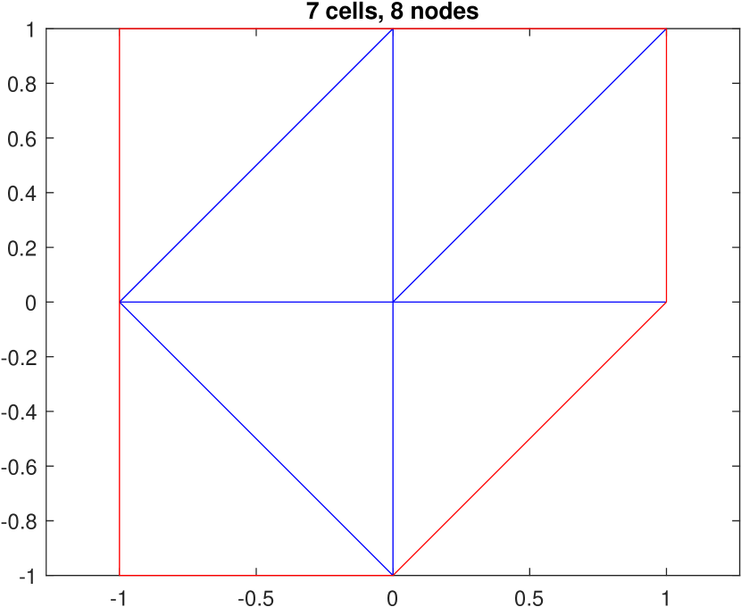
(a) mesh 1

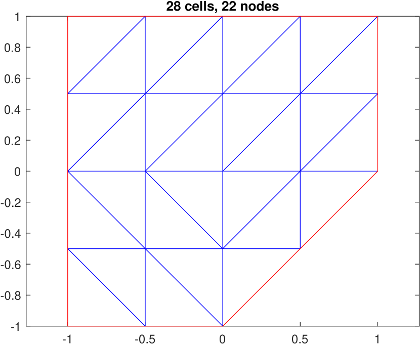
(b) mesh 2

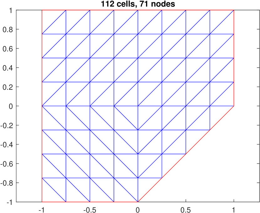
(c) mesh 3

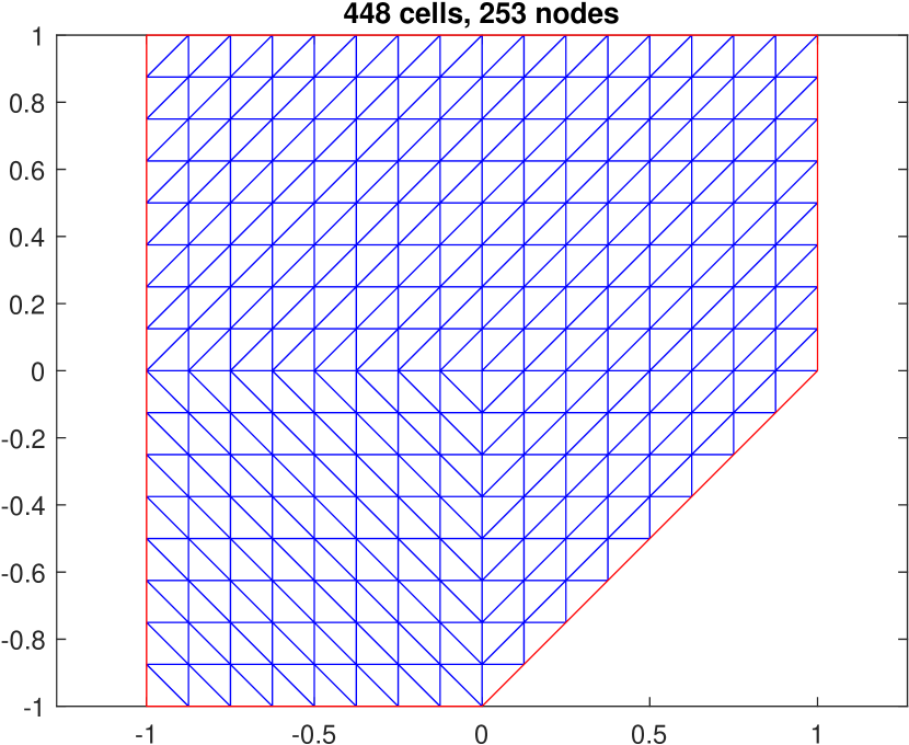
(d) mesh 4

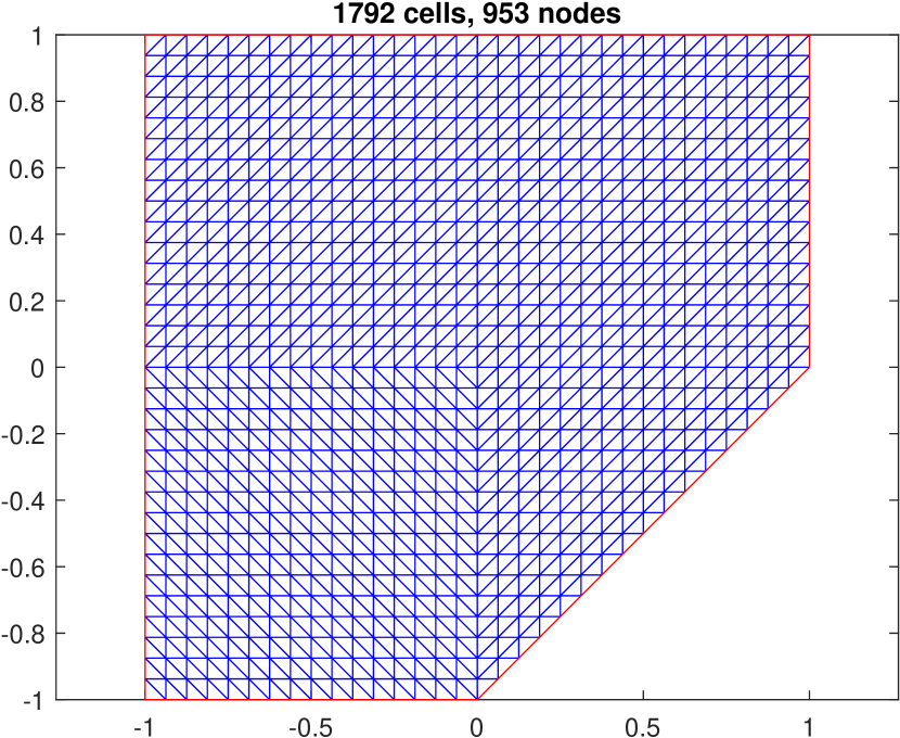
(e) mesh 5

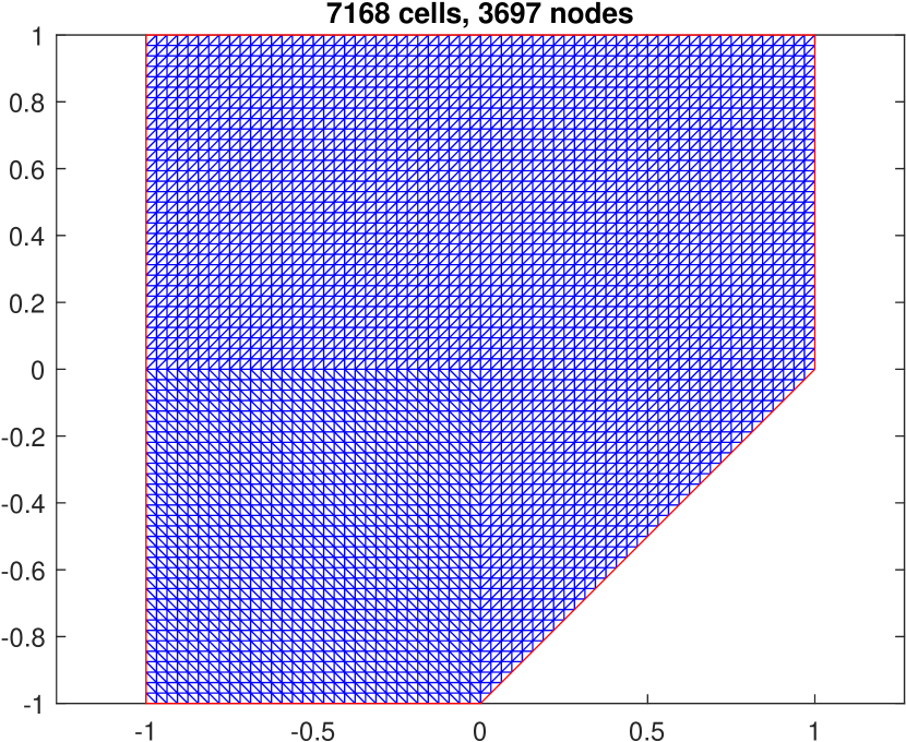
(f) mesh 6

Figure 5.1: Uniformly refined conforming triangular meshes for a 2D polygonal domain.

In the following text, we are going to present our numerical results. For Example 5.1 to 5.3, we take the polygonal domain $\Omega=\left\{(x,y)\big{|}-1\leqslant x,y\leqslant 1,y-x+1\geqslant 0\right\}$ and use the uniformly refined conforming triangular meshes as depicted in Figure 5.1. For simplicity, we only use the Dirichlet boundary condition in our tests. The penalty coefficients for the numerical flux (3.3) are taken to be $\eta=10.0$, and the upwind coefficients $\bm{C}_{12}$ are set according to the MD-LDG scheme [22], with the (constant) auxiliary vector field $\bm{v}_{0}=(1,0)^{T}$. In the following text, we use $\epsilon$ to denote any fixed small positive constant.

Example 5.1.

A Linear Case

In our first example, we take the exact solution to be

$$u(x,y)=e^{\sin(\pi x)}\cos(\pi(x+y)),$$

$$\bm{q}(x,y)=\begin{pmatrix}\pi e^{\sin(\pi x)}\left(\cos(\pi x)\cos(\pi(x+y))-\sin(\pi(x+y))\right)\\ -\pi e^{\sin(\pi x)}\sin(\pi(x+y))\end{pmatrix},$$

$$\bm{\sigma}(x,y)=\begin{pmatrix}\pi e^{\sin(\pi x)}\left(\cos(\pi x)\cos(\pi(x+y))-\sin(\pi(x+y))\right)\\ -\pi e^{\sin(\pi x)}\sin(\pi(x+y))\end{pmatrix},$$

$$f(x,y)=\pi^{2}e^{\sin(\pi x)}\left(\cos(\pi(x+y))\left(2-\cos^{2}(\pi x)+\sin(\pi x)\right)+2\cos(\pi x)\sin(\pi(x+y))\right).$$

We test with $p=2$ to verify the consistency of our gradient descent method for the Poisson equation. The errors are shown in Table 5.1, demonstrating that our solver provides the best convergence in this linear case, when compared to linear LDG error estimates [18]. We also mention that every test here converges within one iteration, which aligns with Remark 3.4 well.

Table 5.1: Error table for Example 5.1. Parameters: $p=2$, $\epsilon=0$, $\delta_{w_{h}}=10^{-16}$, $\delta_{\rho}=10^{-16}$.

$k$	$N_{e}$	$N_{\rm dof}$	$\left\lVert u-u_{h}\right\rVert_{L^{p}}$	order	$\left\lVert\bm{q}-\bm{q}_{h}\right\rVert_{L^{p}}$	order	$\left\lVert\bm{\sigma}-\bm{\sigma}_{h}\right\rVert_{L^{p^{\prime}}}$	order
1	7	21	1.2653e+00	-	1.0916e+01	-	1.0916e+01	-
	28	84	7.0497e-01	0.8438	5.7008e+00	0.9372	5.7008e+00	0.9372
	112	336	2.6383e-01	1.4180	3.4436e+00	0.7272	3.4436e+00	0.7272
	448	1344	7.5449e-02	1.8060	1.8233e+00	0.9174	1.8233e+00	0.9174
	1792	5376	1.9627e-02	1.9427	9.2622e-01	0.9771	9.2622e-01	0.9771
	7168	21504	4.9640e-03	1.9832	4.6540e-01	0.9929	4.6540e-01	0.9929
2	7	42	6.1560e-01	-	5.7034e+00	-	5.7034e+00	-
	28	168	1.4129e-01	2.1233	2.3923e+00	1.2534	2.3923e+00	1.2534
	112	672	2.0681e-02	2.7724	7.1105e-01	1.7504	7.1105e-01	1.7504
	448	2688	2.7014e-03	2.9365	1.8887e-01	1.9126	1.8887e-01	1.9126
	1792	10752	3.4226e-04	2.9805	4.8095e-02	1.9734	4.8095e-02	1.9734
	7168	43008	4.3003e-05	2.9926	1.2087e-02	1.9925	1.2087e-02	1.9925
3	7	70	4.4329e+00	-	4.8816e+00	-	4.8816e+00	-
	28	280	3.5407e-02	3.6118	7.5929e-01	2.6846	7.5929e-01	2.6846
	112	1120	2.7498e-03	3.6866	1.2018e-01	2.6594	1.2018e-01	2.6594
	448	4480	1.7279e-04	3.9922	1.5933e-02	2.9151	1.5933e-02	2.9151
	1792	17920	1.0786e-05	4.0017	2.0237e-03	2.9770	2.0237e-03	2.9770
	7168	71680	6.7332e-07	4.0018	2.5385e-04	2.9950	2.5385e-04	2.9950
4	7	105	1.2932e-01	-	1.5622e+00	-	1.5622e+00	-
	28	420	9.2744e-03	3.8016	2.2166e-01	2.8171	2.2166e-01	2.8171
	112	1680	3.6503e-04	4.6672	1.7668e-02	3.6491	1.7668e-02	3.6491
	448	6720	1.2501e-05	4.8680	1.2025e-03	3.8770	1.2025e-03	3.8770
	1792	26880	3.9980e-07	4.9666	7.6083e-05	3.9824	7.6083e-05	3.9824
	7168	107520	1.2568e-08	4.9914	4.7602e-06	3.9985	4.7602e-06	3.9985
5	7	147	1.1381e-01	-	1.0080e+00	-	1.0080e+00	-
	28	588	2.3911e-03	5.5728	5.5520e-02	4.1824	5.5520e-02	4.1824
	112	2352	5.2502e-05	5.5092	2.4154e-03	4.5227	2.4154e-03	4.5227
	448	9408	8.6522e-07	5.9232	7.9605e-05	4.9232	7.9605e-05	4.9232
	1792	37632	1.3790e-08	5.9714	2.5347e-06	4.9730	2.5347e-06	4.9730
	7168	150528	2.1659e-10	5.9925	7.9403e-08	4.9965	7.9403e-08	4.9965
6	7	196	1.9906e-02	-	4.3179e-01	-	4.3179e-01	-
	28	784	4.0022e-04	5.6363	1.3970e-02	4.9499	1.3970e-02	4.9499
	112	3136	4.0023e-06	6.6438	2.8650e-04	5.6077	2.8650e-04	5.6077
	448	12544	3.5067e-08	6.8346	5.0342e-06	5.8306	5.0342e-06	5.8306
	1792	50176	2.7932e-10	6.9721	7.9191e-08	5.9903	7.9191e-08	5.9903
	7168	200704	2.1943e-12	6.9920	1.2349e-09	6.0028	1.2349e-09	6.0028

Example 5.2.

A Regular Case

We take the radial exact solution [7, 27] as

$$u(x,y)=\frac{p-1}{(\sigma+2)^{\frac{1}{p-1}}}\frac{1-r(x,y)^{\frac{\sigma+p}{p-1}}}{\sigma+p}\in W^{\frac{\sigma+1}{p-1}+\frac{2}{p}+1-\varepsilon,p},$$

$$\bm{q}(x,y)=\begin{pmatrix}-\frac{r(x,y)^{\frac{\sigma+1}{p-1}}}{(\sigma+2)^{\frac{1}{p-1}}}\frac{x}{r(x,y)}\\ -\frac{r(x,y)^{\frac{\sigma+1}{p-1}}}{(\sigma+2)^{\frac{1}{p-1}}}\frac{y}{r(x,y)}\end{pmatrix}\in W^{\frac{\sigma+1}{p-1}+\frac{2}{p}-\varepsilon,p},$$

$$\bm{\sigma}(x,y)=\begin{pmatrix}\frac{-r(x,y)^{\sigma}x}{\sigma+2}\\ \frac{-r(x,y)^{\sigma}y}{\sigma+2}\end{pmatrix}\in W^{\sigma+3-\frac{2}{p}-\varepsilon,p^{\prime}},$$

$$f(x,y)=r(x,y)^{\sigma},$$

where $r(x,y)=\sqrt{x^{2}+y^{2}}$ is the radial distance. Although the exact solution is not smooth, it does not have singular points or zero-gradient regions with positive measures. For tests, we choose the following two groups of parameters, $(\sigma,p)=(0,1.5)$ and $(\sigma,p)=(7,4)$. The errors are listed in Table 5.2 and 5.3 respectively, and some of the convergence history of the nonlinear solver are shown in Figure 5.2 and 5.3.

The convergence rates are going up only some of the way up as $k$ increases, possibly due to limited regularity.

1. Case $(\sigma,p)=(0,1.5)$: $(u,\bm{q},\bm{\sigma})\in W^{s+1-\varepsilon,p}\times W^{s-\varepsilon,p}\times W^{r-\varepsilon,p^{\prime}}$ with $(s,r)=(\frac{10}{3},\frac{5}{3})$. Our scheme attains the best convergence rate for all variables compared to the linear LDG scheme, which coincides with observations from the HDG scheme [27], although in different norms. Moreover, our numerical results coincide with the improved HHO estimates [35, Theorem 1], so we guess this is due to good local regimes of the exact solution.

2. Case $(\sigma,p)=(7,4)$: $(u,\bm{q},\bm{\sigma})\in W^{s+1-\varepsilon,p}\times W^{s-\varepsilon,p}\times W^{r-\varepsilon,p^{\prime}}$ with $(s,r)=(\frac{19}{6},\frac{19}{2})$. The convergence rates for gradient variables $\bm{q}$ and $\bm{\sigma}$ are the best, but that for the primal variable $u$ is not.

Besides, for any $h$ and $k$, both examples consistently require around 15 and 25 iterations respectively, demonstrating $hk$-independent convergence of our preconditioned method.

Table 5.2: Error table for Example 5.2. Parameters: $\sigma=0$, $p=1.5$, $\epsilon=10^{-14}$, $\delta_{w_{h}}=10^{-16}$, $\delta_{\rho}=10^{-16}$.

$k$	$N_{e}$	$N_{\rm dof}$	$\left\lVert u-u_{h}\right\rVert_{L^{p}}$	order	$\left\lVert\bm{q}-\bm{q}_{h}\right\rVert_{L^{p}}$	order	$\left\lVert\bm{\sigma}-\bm{\sigma}_{h}\right\rVert_{L^{p^{\prime}}}$	order
1	7	21	4.5425e-02	-	2.2627e-01	-	3.2533e-01	-
	28	84	1.2729e-02	1.8354	1.2465e-01	0.8601	1.6710e-01	0.9612
	112	336	3.2486e-03	1.9702	6.4513e-02	0.9503	8.4892e-02	0.9770
	448	1344	8.1708e-04	1.9913	3.2663e-02	0.9820	4.2871e-02	0.9856
	1792	5376	2.0453e-04	1.9982	1.6402e-02	0.9938	2.1543e-02	0.9928
	7168	21504	5.1147e-05	1.9996	8.2140e-03	0.9977	1.0796e-02	0.9967
2	7	42	7.7338e-03	-	5.2735e-02	-	9.2414e-02	-
	28	168	8.9019e-04	3.1190	1.3935e-02	1.9200	2.9935e-02	1.6263
	112	672	1.0777e-04	3.0461	3.6288e-03	1.9412	9.7520e-03	1.6181
	448	2688	1.3320e-05	3.0164	9.2595e-04	1.9705	3.1265e-03	1.6412
	1792	10752	1.6624e-06	3.0022	2.3373e-04	1.9861	9.9332e-04	1.6542
	7168	43008	2.0793e-07	2.9990	5.8705e-05	1.9933	3.1419e-04	1.6606
3	7	70	6.7287e-04	-	9.0177e-03	-	1.9052e-02	-
	28	280	5.5204e-05	3.6075	1.5156e-03	2.5729	6.4762e-03	1.5567
	112	1120	3.9437e-06	3.8071	2.1125e-04	2.8428	2.0421e-03	1.6651
	448	4480	2.6731e-07	3.8829	2.8250e-05	2.9026	6.4327e-04	1.6665
	1792	17920	1.7606e-08	3.9244	3.6875e-06	2.9375	2.0247e-04	1.6677
	7168	71680	1.8102e-09	3.2818	4.7462e-07	2.9578	6.3822e-05	1.6656
4	7	105	1.3377e-04	-	1.2196e-03	-	3.0487e-03	-
	28	420	7.9208e-06	4.0780	1.6633e-04	2.8743	9.5295e-04	1.6777
	112	1680	4.2657e-07	4.2148	1.8647e-05	3.1570	3.0028e-04	1.6661
	448	6720	2.1984e-08	4.2783	1.9546e-06	3.2540	9.4582e-05	1.6667
	1792	26880	1.2093e-09	4.1842	1.9903e-07	3.2958	2.9790e-05	1.6667
	7168	107520	1.1226e-09	0.1074	2.1021e-08	3.2431	9.3838e-06	1.6666
5	7	147	2.9285e-05	-	4.6112e-04	-	1.5947e-03	-
	28	588	1.5832e-06	4.2093	5.1172e-05	3.1717	5.0520e-04	1.6584
	112	2352	7.9726e-08	4.3116	5.1633e-06	3.3090	1.5913e-04	1.6666
	448	9408	5.6283e-09	3.8243	5.1460e-07	3.3268	5.0123e-05	1.6667
	1792	37632	5.3178e-09	0.0819	5.7037e-08	3.1735	1.5788e-05	1.6666
	7168	150528	3.7110e-10	3.8410	5.4414e-09	3.3899	4.9727e-06	1.6668
6	7	196	6.8486e-06	-	1.7974e-04	-	6.7422e-04	-
	28	784	3.5864e-07	4.2552	1.8790e-05	3.2579	2.1222e-04	1.6676
	112	3136	1.7881e-08	4.3260	1.8690e-06	3.3296	6.6846e-05	1.6667
	448	12544	2.1894e-09	3.0299	1.8631e-07	3.3265	2.1056e-05	1.6666
	1792	50176	2.0939e-09	0.0644	2.0968e-08	3.1514	6.6326e-06	1.6666
	7168	200704	1.9309e-09	0.1169	6.8024e-09	1.6241	2.0898e-06	1.6662

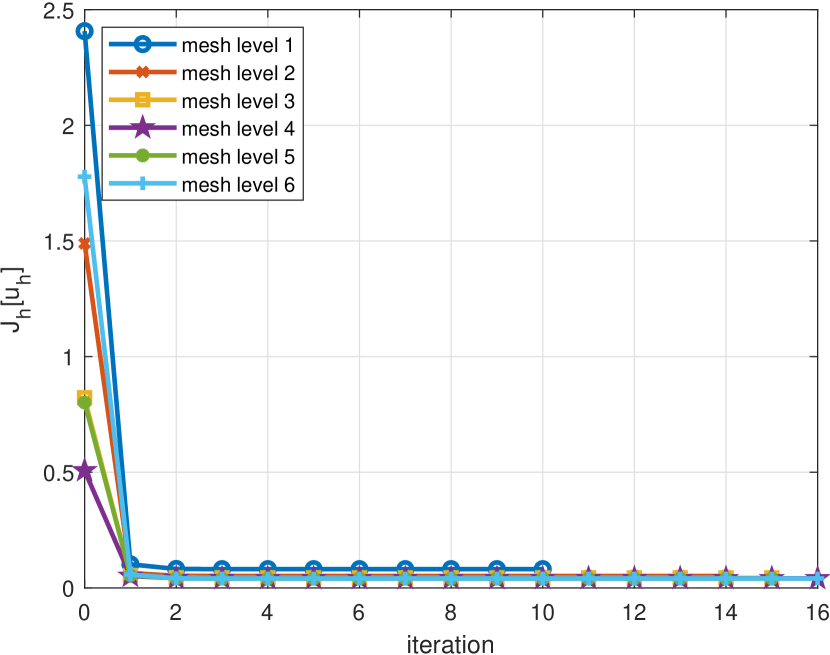
(a) $J_{h}(u_{h})$, $k=1$

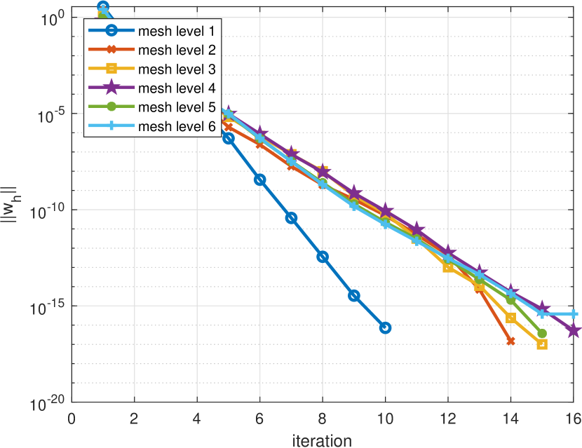
(b) $\left\lVert w_{h}\right\rVert$, $k=1$

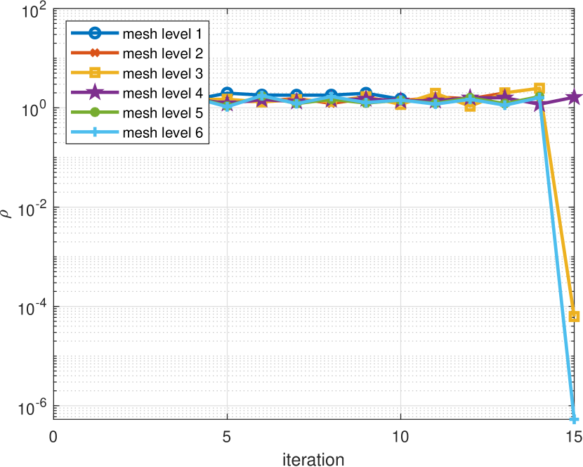
(c) $\rho$, $k=1$

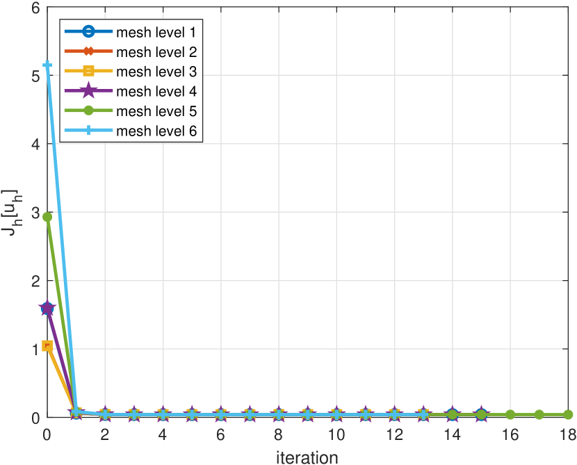
(d) $J_{h}(u_{h})$, $k=6$

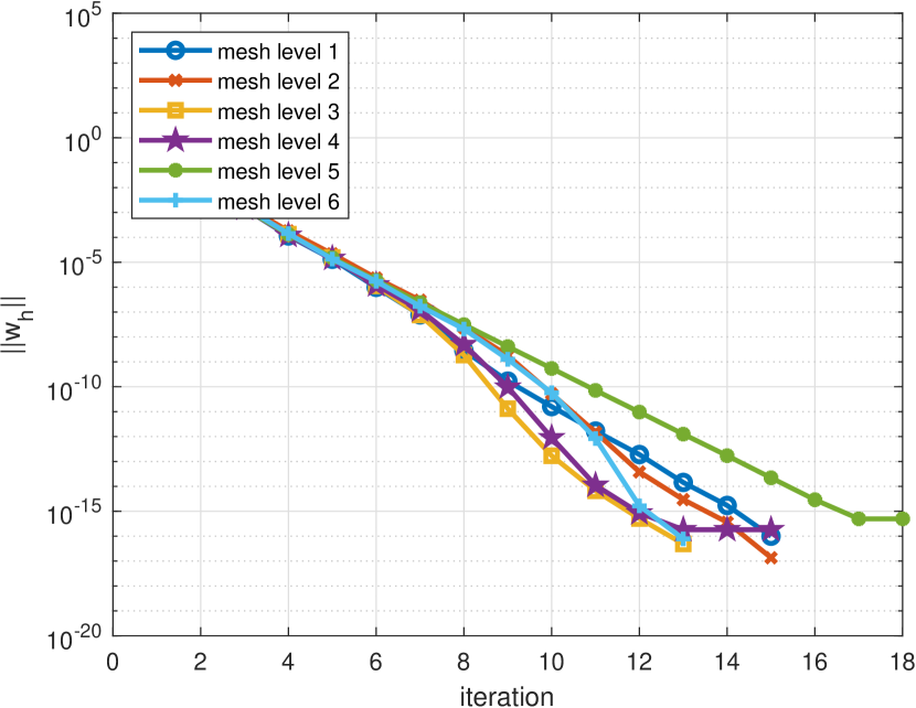
(e) $\left\lVert w_{h}\right\rVert$, $k=6$

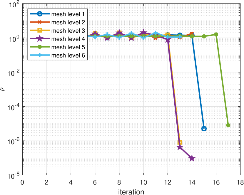
(f) $\rho$, $k=6$

Figure 5.2: Convergence history for Example 5.2, with $\sigma=0$ and $p=1.5$.

Table 5.3: Error table for Example 5.2. Parameters: $\sigma=7$, $p=4$, $\epsilon=10^{-14}$, $\delta_{w_{h}}=10^{-16}$, $\delta_{\rho}=10^{-16}$.

$k$	$N_{e}$	$N_{\rm dof}$	$\left\lVert u-u_{h}\right\rVert_{L^{p}}$	order	$\left\lVert\bm{q}-\bm{q}_{h}\right\rVert_{L^{p}}$	order	$\left\lVert\bm{\sigma}-\bm{\sigma}_{h}\right\rVert_{L^{p^{\prime}}}$	order
1	7	21	1.1225e-01	-	4.5324e-01	-	1.9580e-01	-
	28	84	4.8591e-02	1.2079	2.6553e-01	0.7714	7.0942e-02	1.4647
	112	336	1.2312e-02	1.9806	7.8134e-02	1.7648	3.3611e-02	1.0777
	448	1344	3.3495e-03	1.8781	3.8148e-02	1.0343	1.8592e-02	0.8543
	1792	5376	9.1362e-04	1.8743	1.9966e-02	0.9341	1.0293e-02	0.8530
	7168	21504	2.4744e-04	1.8845	1.0240e-02	0.9634	5.4531e-03	0.9165
2	7	42	9.4888e-02	-	3.9841e-01	-	1.0562e-01	-
	28	168	2.3261e-02	2.0283	1.0691e-01	1.8979	1.8035e-02	2.5499
	112	672	5.3419e-03	2.1225	1.3977e-02	2.9353	2.9171e-03	2.6282
	448	2688	1.1927e-03	2.1631	1.8476e-03	2.9193	5.7511e-04	2.3426
	1792	10752	2.5934e-04	2.2013	3.7062e-04	2.3176	1.3894e-04	2.0494
	7168	43008	5.5541e-05	2.2232	9.0708e-05	2.0306	3.5456e-05	1.9703
3	7	70	3.5097e-02	-	2.2779e-01	-	4.0262e-02	-
	28	280	1.0875e-02	1.6904	4.0079e-02	2.5068	2.9800e-03	3.7560
	112	1120	1.9920e-03	2.4487	4.1837e-03	3.2600	1.9061e-04	3.9667
	448	4480	3.5111e-04	2.5042	4.6552e-04	3.1679	1.4127e-05	3.7540
	1792	17920	6.0286e-05	2.5420	5.1760e-05	3.1689	1.3110e-06	3.4298
	7168	71680	1.0218e-05	2.5608	6.6295e-06	2.9649	1.4394e-07	3.1871
4	7	105	2.4579e-02	-	1.5532e-01	-	1.1192e-02	-
	28	420	4.4327e-03	2.4712	1.0572e-02	3.8770	3.1600e-04	5.1464
	112	1680	6.4281e-04	2.7857	1.1827e-03	3.1601	9.0793e-06	5.1212
	448	6720	8.8926e-05	2.8537	1.3170e-04	3.1667	2.8590e-07	4.9890
	1792	26880	1.2062e-05	2.8821	1.4725e-05	3.1610	1.4783e-08	4.2735
	7168	107520	1.6240e-06	2.8928	4.9436e-05	-1.7473	1.1314e-09	3.7077
5	7	147	1.2837e-02	-	6.6089e-02	-	2.4940e-03	-
	28	588	2.7142e-03	2.2417	6.4898e-03	3.3482	4.2796e-05	5.8648
	112	2352	3.0470e-04	3.1551	7.2250e-04	3.1671	6.5958e-07	6.0198
	448	9408	3.3073e-05	3.2036	8.0512e-05	3.1657	1.0836e-08	5.9276
	1792	37632	3.5545e-06	3.2180	8.9970e-06	3.1617	2.0937e-09	2.3718
	7168	150528	3.7845e-07	3.2315	1.0077e-06	3.1584	4.4897e-09	-1.1006
6	7	196	5.6444e-03	-	3.3924e-02	-	4.2407e-04	-
	28	784	7.2374e-04	2.9633	2.8283e-03	3.5843	2.1715e-06	7.6095
	112	3136	6.2957e-05	3.5230	3.1497e-04	3.1666	1.7375e-08	6.9656
	448	12544	5.3619e-06	3.5535	3.4873e-05	3.1751	5.0282e-09	1.7889
	1792	50176	4.5741e-07	3.5512	3.8761e-06	3.1694	1.0701e-08	-1.0897
	7168	200704	8.3135e-08	2.4600	5.5058e-06	-0.5064	2.3028e-09	2.2163

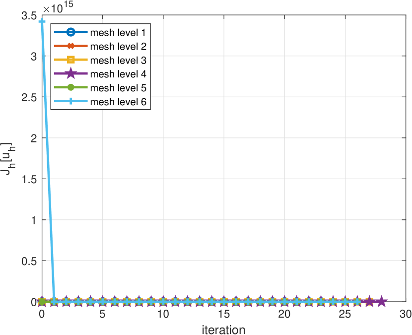
(a) $J_{h}(u_{h})$, $k=1$

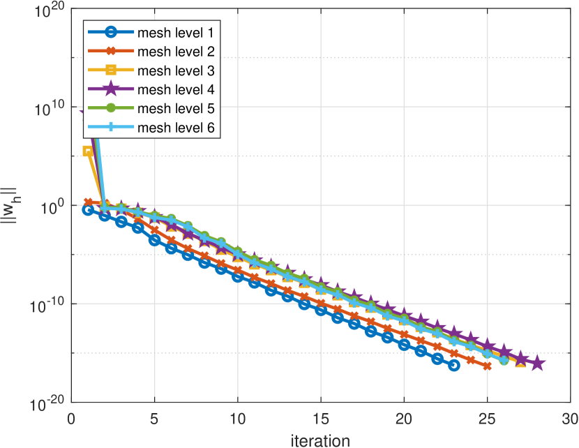
(b) $\left\lVert w_{h}\right\rVert$, $k=1$

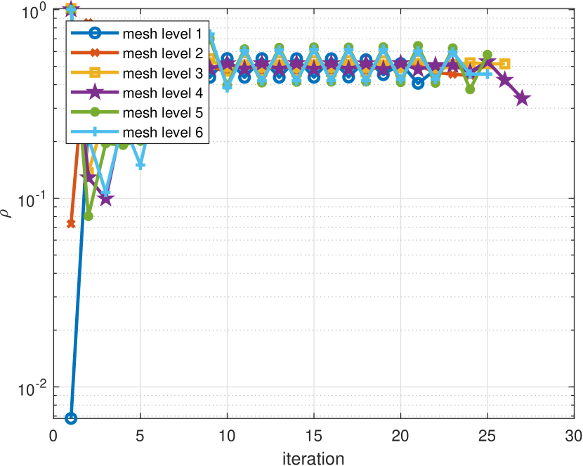
(c) $\rho$, $k=1$

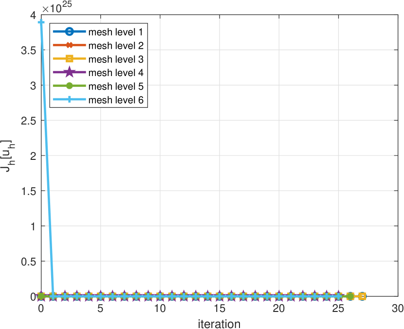
(d) $J_{h}(u_{h})$, $k=6$

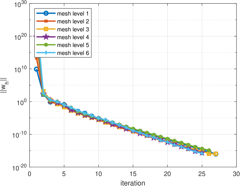
(e) $\left\lVert w_{h}\right\rVert$, $k=6$

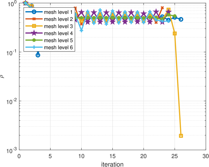
(f) $\rho$, $k=6$

Figure 5.3: Convergence history for Example 5.2, with $\sigma=7$ and $p=4$.

Example 5.3.

A Degenerate Case

We take the radial exact solution [7] to be

$$u(x,y)=\begin{cases}0,&r(x,y)<a,\\ (r(x,y)-a)^{4},&r(x,y)\geqslant a,\end{cases}\in W^{4,\infty}\cap W^{4+\frac{1}{p}-\varepsilon,p},$$

$$\bm{q}(x,y)=\begin{cases}\bm{0},&r(x,y)<a,\\ \begin{pmatrix}4(r(x,y)-a)^{3}\frac{x}{r(x,y)}\\ 4(r(x,y)-a)^{3}\frac{y}{r(x,y)}\end{pmatrix},&r(x,y)\geqslant a,\end{cases}\in W^{3,\infty}\cap W^{3+\frac{1}{p}-\varepsilon,p},$$

$$\bm{\sigma}(x,y)=\begin{cases}\bm{0},&r(x,y)<a,\\ \begin{pmatrix}4^{p-1}(r(x,y)-a)^{3p-3}\frac{x}{r(x,y)}\\ 4^{p-1}(r(x,y)-a)^{3p-3}\frac{y}{r(x,y)}\end{pmatrix},&r(x,y)\geqslant a,\end{cases}\in W^{3p-3,\infty}\cap W^{3p-2-\frac{1}{p}-\varepsilon,p^{\prime}},$$

$$f(x,y)=\begin{cases}0,&r(x,y)<a,\\ 4^{p-1}(r(x,y)-a)^{3p-4}\left(2-3p+\frac{a}{r(x,y)}\right),&r(x,y)\geqslant a.\end{cases}$$

The gradient vanishes on $B_{a}(\bm{0})$, so the problem is degenerate when $p>2$. Just as in the article [7], we choose $a=0.3$ and $p=4$. The results are shown in Table 5.4 and Figure 5.4. The number of iterations is around 25 for most $h$’s and $k$’s.

In this example, $(u,\bm{q},\bm{\sigma})\in W^{s+1-\varepsilon,p}\times W^{s-\varepsilon,p}\times W^{r-\varepsilon,p^{\prime}}$ with $(s,r)=(3.25,9.75)$. The convergence rates are around the best values for $\bm{q}$ and $\bm{\sigma}$ in comparison to the linear case.

Table 5.4: Error table for Example 5.3. Parameters: $p=4$, $\epsilon=10^{-14}$, $\delta_{w_{h}}=10^{-16}$, $\delta_{\rho}=10^{-16}$.

$k$	$N_{e}$	$N_{\rm dof}$	$\left\lVert u-u_{h}\right\rVert_{L^{p}}$	order	$\left\lVert\bm{q}-\bm{q}_{h}\right\rVert_{L^{p}}$	order	$\left\lVert\bm{\sigma}-\bm{\sigma}_{h}\right\rVert_{L^{p^{\prime}}}$	order
1	7	21	5.0087e-01	-	2.1984e+00	-	1.2909e+01	-
	28	84	1.9990e-01	1.3252	1.1516e+00	0.9328	6.0890e+00	1.0841
	112	336	6.4463e-02	1.6327	5.1304e-01	1.1665	2.3958e+00	1.3457
	448	1344	1.7066e-02	1.9173	1.9450e-01	1.3993	1.2788e+00	0.9057
	1792	5376	4.6698e-03	1.8697	1.0157e-01	0.9373	7.1692e-01	0.8349
	7168	21504	1.2687e-03	1.8799	5.2588e-02	0.9497	3.8597e-01	0.8933
2	7	42	3.4929e-01	-	1.5828e+00	-	1.0810e+01	-
	28	168	1.4205e-01	1.2981	8.1954e-01	0.9496	2.0331e+00	2.4106
	112	672	3.0138e-02	2.2367	1.4992e-01	2.4506	3.5512e-01	2.5173
	448	2688	6.8604e-03	2.1352	1.6884e-02	3.1505	6.4558e-02	2.4596
	1792	10752	1.5120e-03	2.1819	2.8383e-03	2.5726	1.4676e-02	2.1372
	7168	43008	3.2590e-04	2.2140	6.7299e-04	2.0764	3.7017e-03	1.9872
3	7	70	3.0707e-01	-	1.5849e+00	-	5.5966e+00	-
	28	280	7.2396e-02	2.0846	4.8447e-01	1.7099	5.2846e-01	3.4047
	112	1120	1.2841e-02	2.4951	4.8259e-02	3.3275	3.7767e-02	3.8066
	448	4480	2.3307e-03	2.4620	4.0781e-03	3.5648	2.5268e-03	3.9017
	1792	17920	4.0573e-04	2.5222	3.7353e-04	3.4486	2.0165e-04	3.6474
	7168	71680	6.9167e-05	2.5524	1.6427e-04	1.1851	2.0028e-05	3.3318
4	7	105	1.1334e-01	-	9.1652e-01	-	2.2549e+00	-
	28	420	3.2154e-02	1.8176	1.6407e-01	2.4819	1.0525e-01	4.4211
	112	1680	4.8426e-03	2.7312	1.4662e-02	3.4842	2.9308e-03	5.1664
	448	6720	6.9000e-04	2.8111	1.6002e-03	3.1957	8.9106e-05	5.0396
	1792	26880	9.4671e-05	2.8656	2.6576e-04	2.5901	3.0897e-06	4.8500
	7168	107520	1.2770e-05	2.8902	1.0274e-04	1.3711	7.3647e-07	2.0688
5	7	147	8.6038e-02	-	5.7931e-01	-	7.9631e-01	-
	28	588	2.2907e-02	1.9092	7.2822e-02	2.9919	1.9460e-02	5.3547
	112	2352	2.6796e-03	3.0957	5.0373e-03	3.8536	3.1838e-04	5.9336
	448	9408	2.9864e-04	3.1656	6.1208e-04	3.0409	5.0076e-06	5.9905
	1792	37632	3.2344e-05	3.2068	6.5927e-05	3.2148	2.2571e-07	4.4716
	7168	150528	3.4570e-06	3.2259	8.1953e-05	-0.3139	2.7001e-07	-0.2585
6	7	196	4.9951e-02	-	4.3889e-01	-	1.9182e-01	-
	28	784	7.6588e-03	2.7053	2.5296e-02	4.1169	1.8994e-03	6.6581
	112	3136	6.9588e-04	3.4602	2.9030e-03	3.1233	1.1439e-05	7.3754
	448	12544	6.0415e-05	3.5259	2.9858e-04	3.2814	4.7298e-07	4.5961
	1792	50176	5.2296e-06	3.5301	1.3389e-04	1.1571	3.3386e-07	0.5025
	7168	200704	5.9421e-07	3.1377	4.6034e-05	1.5403	1.8878e-07	0.8225

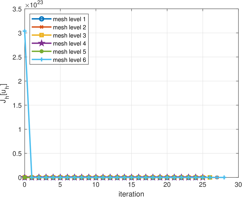
(a) $J_{h}(u_{h})$, $k=1$

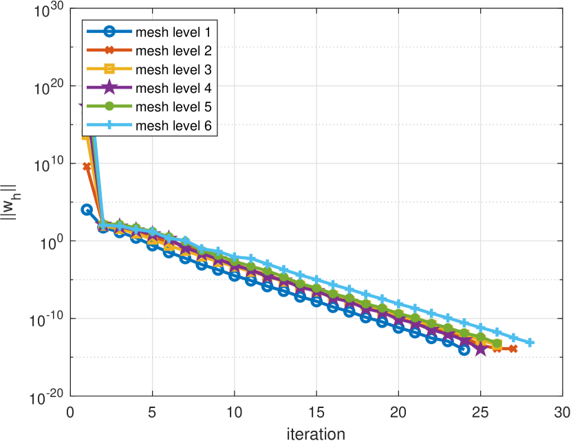
(b) $\left\lVert w_{h}\right\rVert$, $k=1$

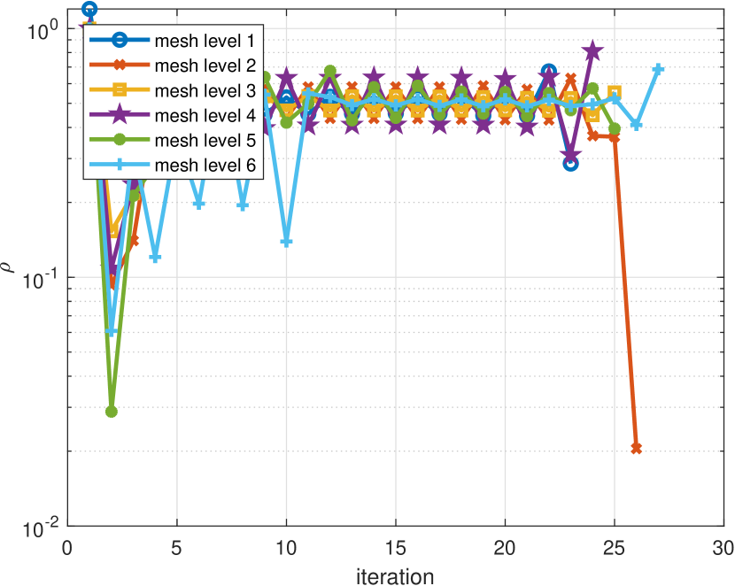
(c) $\rho$, $k=1$

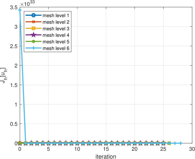
(d) $J_{h}(u_{h})$, $k=6$

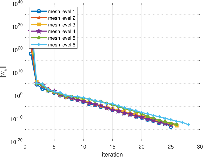
(e) $\left\lVert w_{h}\right\rVert$, $k=6$

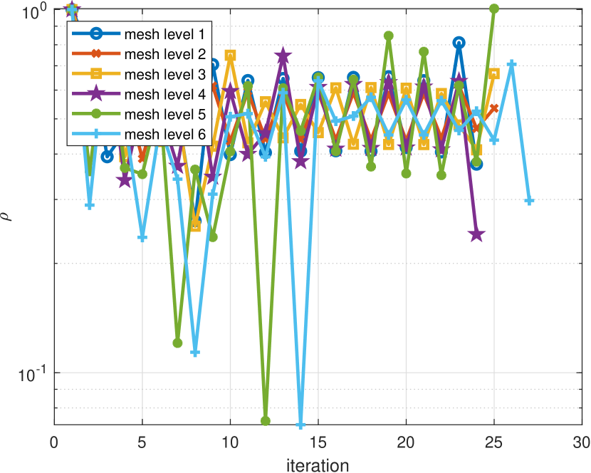
(f) $\rho$, $k=6$

Figure 5.4: Convergence history for Example 5.3, with $p=4$.

Example 5.4.

A Smooth Case

Take the square domain $\Omega=[1,2]^{2}$, and take the radial $p$-harmonic exact solution [47, 27] to be

$$u(x,y)=r(x,y)^{\frac{p-2}{p-1}},$$

$$\bm{q}(x,y)=\begin{pmatrix}\frac{p-2}{p-1}r(x,y)^{\frac{-p}{p-1}}x\\ \frac{p-2}{p-1}r(x,y)^{\frac{-p}{p-1}}y\end{pmatrix},$$

$$\bm{\sigma}(x,y)=\begin{pmatrix}\mathrm{sgn}(p-2)\left\lvert\frac{p-2}{p-1}\right\rvert^{p-1}\frac{x}{r(x,y)^{2}}\\ \mathrm{sgn}(p-2)\left\lvert\frac{p-2}{p-1}\right\rvert^{p-1}\frac{y}{r(x,y)^{2}}\end{pmatrix},$$

$$f(x,y)=0.$$

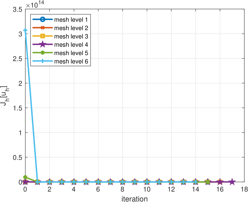
(a) $J_{h}(u_{h})$, $k=1$

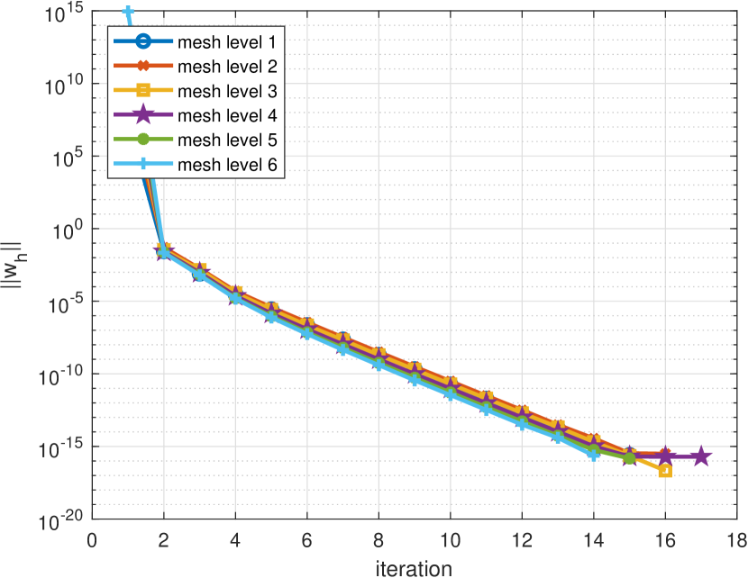
(b) $\left\lVert w_{h}\right\rVert$, $k=1$

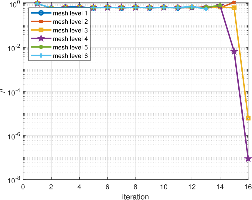
(c) $\rho$, $k=1$

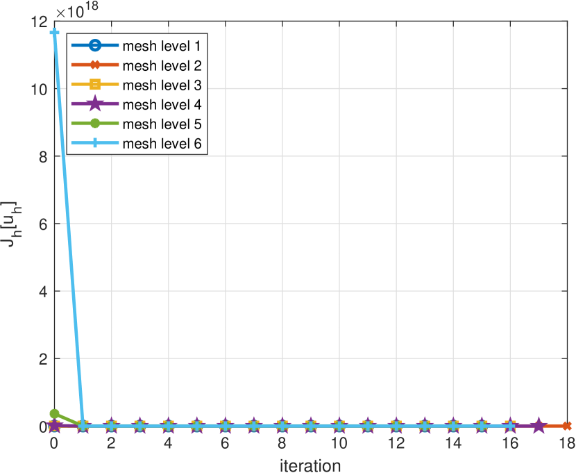
(d) $J_{h}(u_{h})$, $k=6$

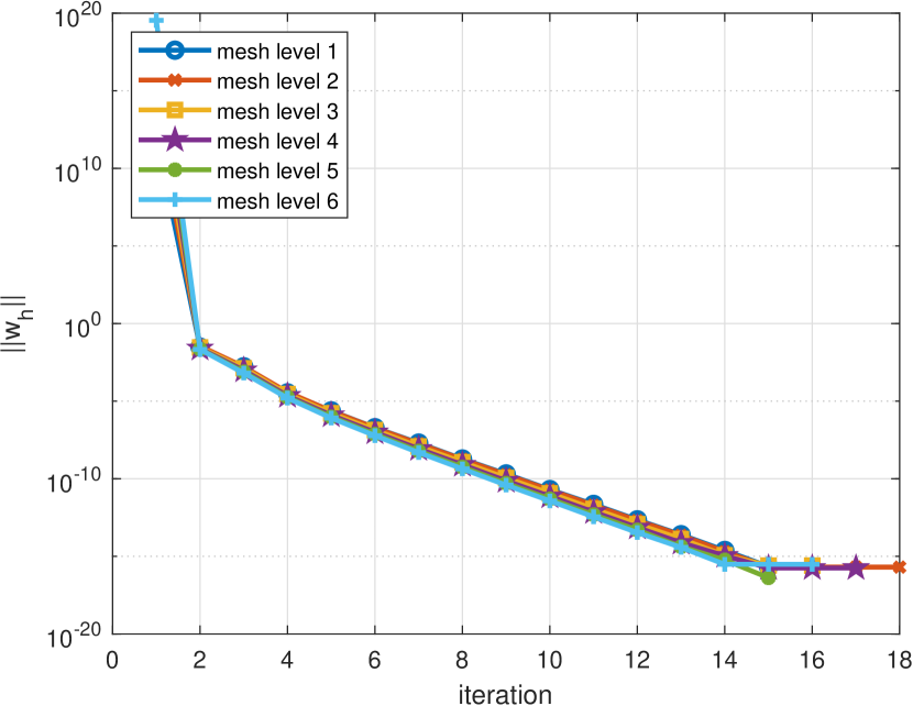
(e) $\left\lVert w_{h}\right\rVert$, $k=6$

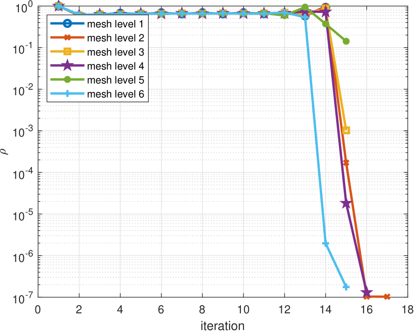
(f) $\rho$, $k=6$

Figure 5.6: Convergence history for Example 5.4, with $p=3$.

This solution is smooth, and moreover its gradient is bounded from both above and below in the domain. We use the same parameters as in the article [27], $p=1.5$ and $p=3$. For both tests, a series of uniformly refined conforming triangular meshes is used. The numerical results for $p=1.5$ and $p=3$ are reported in Table 5.5 with Figure 5.5 and Table 5.6 with Figure 5.6. The number of iterations of these two cases is all around 15, which indicates independence of $h$ and $k$.

The failure to reduce the error when $k$ is big or $h$ is small is possibly due to early termination of the gradient descent iteration and floating-point underflow. For small $k$’s, the results show the best convergence rates for all variables both when $p=1.5$ and when $p=3$, compared against the linear case. Similar results are also observed with the HDG method [27].

Table 5.5: Error table for Example 5.4. Parameters: $p=1.5$, $\epsilon=10^{-14}$, $\delta_{w_{h}}=10^{-16}$, $\delta_{\rho}=10^{-16}$.

$k$	$N_{e}$	$N_{\rm dof}$	$\left\lVert u-u_{h}\right\rVert_{L^{p}}$	order	$\left\lVert\bm{q}-\bm{q}_{h}\right\rVert_{L^{p}}$	order	$\left\lVert\bm{\sigma}-\bm{\sigma}_{h}\right\rVert_{L^{p^{\prime}}}$	order
1	16	48	1.0372e-03	-	2.8342e-02	-	4.1536e-02	-
	64	192	2.7955e-04	1.8915	1.4451e-02	0.9718	2.2825e-02	0.8638
	256	768	7.0869e-05	1.9799	7.2741e-03	0.9903	1.1631e-02	0.9726
	1024	3072	1.7819e-05	1.9917	3.6433e-03	0.9975	5.8448e-03	0.9928
	4096	12288	4.4670e-06	1.9960	1.8226e-03	0.9992	2.9266e-03	0.9979
	16384	49152	1.1181e-06	1.9983	9.1150e-04	0.9997	1.4640e-03	0.9993
2	16	96	8.6236e-05	-	2.2770e-03	-	3.8375e-03	-
	64	384	1.0855e-05	2.9899	5.6497e-04	2.0109	1.0040e-03	1.9344
	256	1536	1.3526e-06	3.0046	1.4138e-04	1.9986	2.5810e-04	1.9598
	1024	6144	1.6836e-07	3.0061	3.5423e-05	1.9968	6.5469e-05	1.9790
	4096	24576	2.0987e-08	3.0040	8.8690e-06	1.9979	1.6488e-05	1.9894
	16384	98304	2.6235e-09	2.9999	2.2191e-06	1.9988	4.1371e-06	1.9947
3	16	160	4.6017e-06	-	1.5681e-04	-	3.3194e-04	-
	64	640	2.6963e-07	4.0931	1.9628e-05	2.9980	4.1896e-05	2.9860
	256	2560	1.6227e-08	4.0545	2.4526e-06	3.0005	5.2193e-06	3.0049
	1024	10240	1.0227e-09	3.9879	3.0633e-07	3.0012	6.5041e-07	3.0045
	4096	40960	5.3706e-10	0.9292	3.9702e-08	2.9478	8.1706e-08	2.9928
	16384	163840	2.2090e-10	1.2817	6.2691e-09	2.6629	1.1142e-08	2.8745
4	16	240	2.5374e-07	-	1.0718e-05	-	2.4662e-05	-
	64	960	7.9948e-09	4.9882	6.7138e-07	3.9967	1.5550e-06	3.9872
	256	3840	2.6664e-10	4.9061	4.1716e-08	4.0085	9.5916e-08	4.0190
	1024	15360	5.1579e-11	2.3700	2.9589e-09	3.8175	6.0748e-09	3.9809
	4096	61440	3.4557e-10	-2.7441	5.1145e-09	-0.7895	7.6760e-09	-0.3375
	16384	245760	1.1062e-11	4.9653	2.1556e-10	4.5685	5.9605e-10	3.6868
5	16	336	1.3848e-08	-	7.8500e-07	-	2.0262e-06	-
	64	1344	2.3354e-10	5.8899	2.5019e-08	4.9716	6.4595e-08	4.9712
	256	5376	3.9682e-10	-0.7648	5.7921e-09	2.1109	8.2972e-09	2.9607
	1024	21504	3.5467e-10	0.1620	8.0309e-09	-0.4715	1.1609e-08	-0.4846
	4096	86016	4.3664e-10	-0.3000	6.1614e-09	0.3823	9.2395e-09	0.3294
	16384	344064	9.1259e-11	2.2584	2.0321e-09	1.6003	3.6673e-09	1.3331
6	16	448	8.4207e-10	-	5.6059e-08	-	1.3230e-07	-
	64	1792	1.8888e-10	2.1564	3.0439e-09	4.2029	5.0056e-09	4.7241
	256	7168	2.2991e-10	-0.2836	5.5574e-09	-0.8685	8.3898e-09	-0.7451
	1024	28672	2.8080e-10	-0.2885	6.6446e-09	-0.2578	9.9341e-09	-0.2438
	4096	114688	1.5732e-10	0.8359	3.4252e-09	0.9560	5.8425e-09	0.7658
	16384	458752	2.9352e-10	-0.8998	4.5425e-09	-0.4073	6.7507e-09	-0.2085

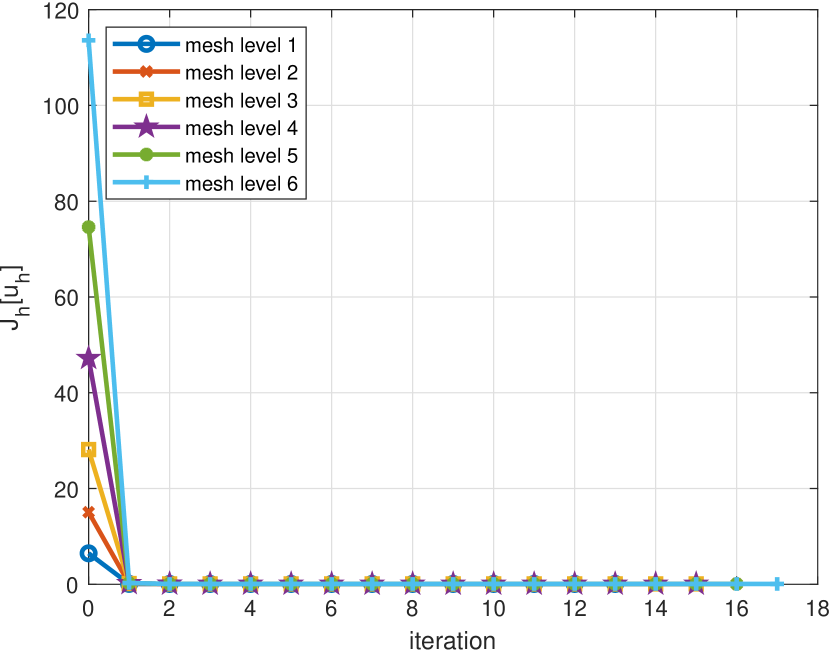
(a) $J_{h}(u_{h})$, $k=1$

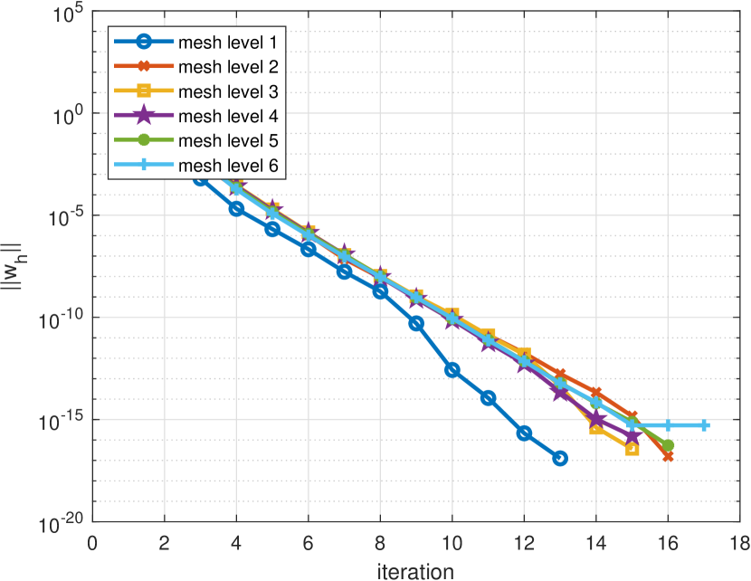
(b) $\left\lVert w_{h}\right\rVert$, $k=1$

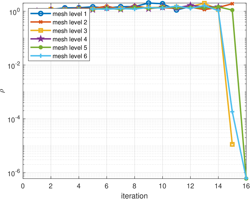
(c) $\rho$, $k=1$

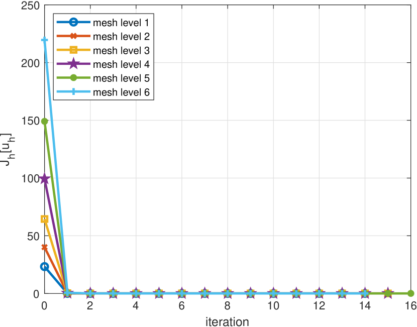
(d) $J_{h}(u_{h})$, $k=6$

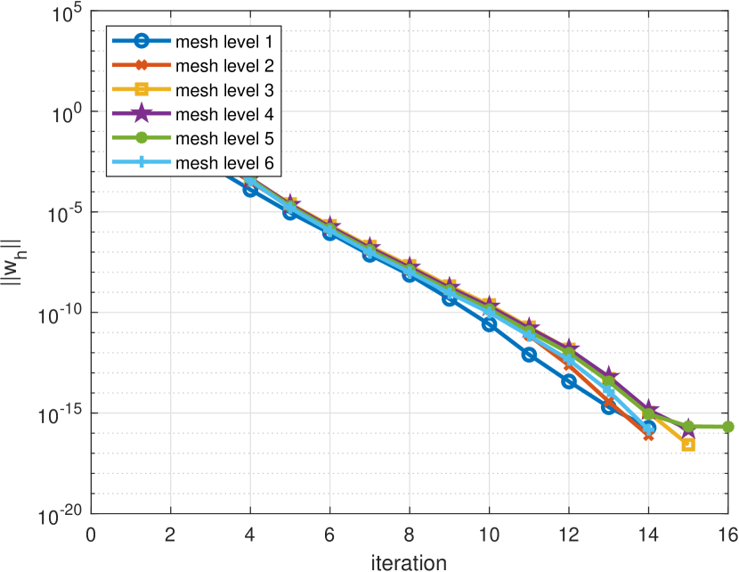
(e) $\left\lVert w_{h}\right\rVert$, $k=6$

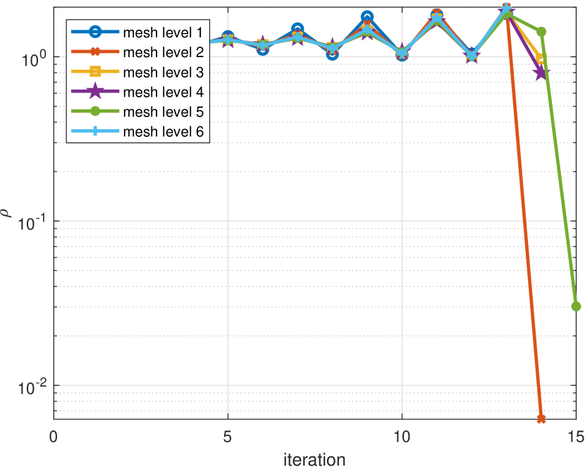
(f) $\rho$, $k=6$

Figure 5.5: Convergence history for Example 5.4, with $p=1.5$.

Table 5.6: Error table for Example 5.4. Parameters: $p=3$, $\epsilon=10^{-14}$, $\delta_{w_{h}}=10^{-16}$, $\delta_{\rho}=10^{-16}$.

$k$	$N_{e}$	$N_{\rm dof}$	$\left\lVert u-u_{h}\right\rVert_{L^{p}}$	order	$\left\lVert\bm{q}-\bm{q}_{h}\right\rVert_{L^{p}}$	order	$\left\lVert\bm{\sigma}-\bm{\sigma}_{h}\right\rVert_{L^{p^{\prime}}}$	order
1	16	48	6.1661e-04	-	8.3824e-03	-	2.8982e-03	-
	64	192	1.6146e-04	1.9332	4.3914e-03	0.9327	1.5995e-03	0.8576
	256	768	4.1832e-05	1.9485	2.2942e-03	0.9367	8.3392e-04	0.9396
	1024	3072	1.0638e-05	1.9753	1.1691e-03	0.9727	4.2445e-04	0.9743
	4096	12288	2.6789e-06	1.9896	5.8994e-04	0.9867	2.1433e-04	0.9857
	16384	49152	6.7208e-07	1.9949	2.9635e-04	0.9933	1.0787e-04	0.9905
2	16	96	2.2017e-05	-	5.2367e-04	-	1.8345e-04	-
	64	384	2.9965e-06	2.8773	1.4110e-04	1.8919	4.9821e-05	1.8805
	256	1536	3.8253e-07	2.9696	3.6936e-05	1.9336	1.3101e-05	1.9271
	1024	6144	4.8458e-08	2.9808	9.4465e-06	1.9672	3.3450e-06	1.9696
	4096	24576	6.1051e-09	2.9886	2.3870e-06	1.9846	8.4330e-07	1.9879
	16384	98304	1.0885e-09	2.4877	5.9969e-07	1.9929	2.1182e-07	1.9932
3	16	160	1.1969e-06	-	3.4546e-05	-	1.1652e-05	-
	64	640	7.9547e-08	3.9114	4.5249e-06	2.9326	1.5044e-06	2.9533
	256	2560	5.0486e-09	3.9779	5.7407e-07	2.9786	1.9013e-07	2.9841
	1024	10240	3.9896e-10	3.6616	7.3632e-08	2.9628	2.4486e-08	2.9569
	4096	40960	2.5694e-10	0.6348	2.2007e-08	1.7424	4.9171e-09	2.3161
	16384	163840	1.4915e-10	0.7847	5.5353e-09	1.9912	2.0881e-09	1.2356
4	16	240	7.8745e-08	-	2.3821e-06	-	6.6297e-07	-
	64	960	2.6198e-09	4.9097	1.5224e-07	3.9679	4.2029e-08	3.9795
	256	3840	2.1988e-10	3.5747	2.6166e-08	2.5405	5.3147e-09	2.9833
	1024	15360	3.0472e-10	-0.4708	3.1129e-08	-0.2506	6.5733e-09	-0.3066
	4096	61440	5.1319e-10	-0.7520	4.1770e-08	-0.4242	8.8976e-09	-0.4368
	16384	245760	2.5162e-10	1.0283	2.1292e-08	0.9722	3.6182e-09	1.2981
5	16	336	4.8088e-09	-	1.7436e-07	-	4.0116e-08	-
	64	1344	2.0183e-10	4.5745	1.4229e-08	3.6151	2.8580e-09	3.8111
	256	5376	3.7226e-10	-0.8832	3.1367e-08	-1.1405	6.5744e-09	-1.2019
	1024	21504	3.2134e-10	0.2122	2.2226e-08	0.4970	5.7904e-09	0.1832
	4096	86016	3.8469e-10	-0.2596	1.4881e-08	0.5788	5.9937e-09	-0.0498
	16384	344064	9.6647e-10	-1.3290	4.2430e-08	-1.5117	1.3583e-08	-1.1803
6	16	448	5.0749e-10	-	1.9293e-08	-	7.7938e-09	-
	64	1792	3.5543e-10	0.5138	1.5875e-08	0.2813	7.2192e-09	0.1105
	256	7168	4.1596e-10	-0.2269	1.9329e-08	-0.2840	8.0760e-09	-0.1618
	1024	28672	3.9734e-10	0.0661	1.7754e-08	0.1226	6.7155e-09	0.2661
	4096	114688	1.4872e-10	1.4177	6.3673e-09	1.4794	2.3250e-09	1.5303
	16384	458752	9.0933e-10	-2.6122	5.7407e-08	-3.1725	7.6649e-09	-1.7211

6 Conclusion

In this work, we study the high-order LDG method for the $p$-Laplace equation. Inspired by the variational minimization form of the PDE, we solve a discrete minimization problem instead of the original discrete weak problem to enhance stability, and a specially designed weighted preconditioner is employed to accelerate the nonlinear solver. In our analysis, we rigorously establish the solvability and equivalence between the discrete minimization problem and the original LDG scheme. For the first time, we provide (though non-optimal) a priori error estimates for arbitrarily high-order polynomials under the assumption that the exact solution has sufficient regularity. Our error estimates demonstrate the expected potential for the LDG scheme to achieve high-order accuracy under reasonable assumptions, and the distance functional in our error estimates is non-equivalent to previous works. Moreover, under the same regularity assumption for the primal variable $u$ and using sufficiently high-order polynomials, our estimated convergence rate is the same as that of HHO methods and similar to that of HDG methods. Our numerical results exhibit the best convergence rates for gradient variables in the LDG setting in most cases, while optimal convergence rates are obtained for the primal variable when $1<p\leqslant 2$, which may be attributed to good local regimes. Additionally, the nonlinear solver achieves its desired $hk$-independent number of iterations, as shown in numerical examples. Possible future work includes improvements on the error estimates via dual arguments and via the local regime analysis.

References

- [1] Mark Ainsworth, Gaelle Andriamaro and Oleg Davydov “Bernstein-Bézier Finite Elements of Arbitrary Order and Optimal Assembly Procedures” In SIAM Journal on Scientific Computing 33.6, 2011, pp. 3087–3109 DOI: 10.1137/11082539X
- [2] Mark Ainsworth and David Kay “The Approximation Theory for the -Version Finite Element Method and Application to Non-Linear Elliptic PDEs” In Numerische Mathematik 82.3, 1999, pp. 351–388 DOI: 10.1007/s002110050423
- [3] Mark Ainsworth and David Kay “Approximation Theory for the -Version Finite Element Method and Application to the Non-Linear Laplacian” In Applied Numerical Mathematics 34.4, 2000, pp. 329–344 DOI: 10.1016/S0168-9274(99)00040-9
- [4] Douglas Norman Arnold, Franco Brezzi, Bernardo Cockburn and Luisa Donatella Marini “Discontinuous Galerkin Methods for Elliptic Problems” In Discontinuous Galerkin Methods 11, Lecture Notes in Computational Science and Engineering Berlin, Heidelberg: Springer Berlin Heidelberg, 2000, pp. 89–101 DOI: 10.1007/978-3-642-59721-3˙5
- [5] Douglas Norman Arnold, Franco Brezzi, Bernardo Cockburn and Luisa Donatella Marini “Unified Analysis of Discontinuous Galerkin Methods for Elliptic Problems” In SIAM Journal on Numerical Analysis 39.5, 2002, pp. 1749–1779 DOI: 10.1137/S0036142901384162
- [6] Ivo Babuška and Miloš Zlámal “Nonconforming Elements in the Finite Element Method with Penalty” In SIAM Journal on Numerical Analysis 10.5, 1973, pp. 863–875 DOI: 10.1137/0710071
- [7] John W. Barrett and Wenbin Liu “Finite Element Approximation of the -Laplacian” In Mathematics of Computation 61.204, 1993, pp. 523–537 DOI: 10.1090/S0025-5718-1993-1192966-4
- [8] Francesco Bassi and Stefano Rebay “A High-Order Accurate Discontinuous Finite Element Method for the Numerical Solution of the Compressible Navier-Stokes Equations” In Journal of Computational Physics 131.2, 1997, pp. 267–279 DOI: 10.1006/jcph.1996.5572
- [9] Liudmila Belenki, Lars Diening and Christian Kreuzer “Optimality of an Adaptive Finite Element Method for the -Laplacian Equation” In IMA Journal of Numerical Analysis 32.2, 2012, pp. 484–510 DOI: 10.1093/imanum/drr016
- [10] Jiří Benedikt, Petr Girg, Lukáš Kotrla and Peter Takáč “Origin of the -Laplacian and A. Missbach” In Electronic Journal of Differential Equations 2018.16, 2018, pp. 1–17 URL: https://ejde.math.txstate.edu/Volumes/2018/16/benedikt.pdf
- [11] Rodolfo Bermejo and Juan-Antonio Infante “A Multigrid Algorithm for the -Laplacian” In SIAM Journal on Scientific Computing 21.5, 2000, pp. 1774–1789 DOI: 10.1137/S1064827598339098
- [12] Mark G. Blyth and Constantine Pozrikidis “A Lobatto Interpolation Grid over the Triangle” In IMA Journal of Applied Mathematics 71.1, 2006, pp. 153–169 DOI: 10.1093/imamat/hxh077
- [13] Ignace Bogaert “Iteration-Free Computation of Gauss-Legendre Quadrature Nodes and Weights” In SIAM Journal on Scientific Computing 36.3, 2014, pp. A1008–A1026 DOI: 10.1137/140954969
- [14] Annalisa Buffa and Christoph Ortner “Compact Embeddings of Broken Sobolev Spaces and Applications” In IMA Journal of Numerical Analysis 29.4, 2009, pp. 827–855 DOI: 10.1093/imanum/drn038
- [15] Erik Burman and Alexandre Ern “Discontinuous Galerkin Approximation with Discrete Variational Principle for the Nonlinear Laplacian” In Comptes Rendus Mathematique 346.17-18, 2008, pp. 1013–1016 DOI: 10.1016/j.crma.2008.07.005
- [16] Vicent Caselles, Jean-Michel Morel and Catalina Sbert “An Axiomatic Approach to Image Interpolation” In IEEE Transactions on Image Processing 7.3, 1998, pp. 376–386 DOI: 10.1109/83.661188
- [17] Paul Castillo “Performance of Discontinuous Galerkin Methods for Elliptic PDEs” In SIAM Journal on Scientific Computing 24.2, 2002, pp. 524–547 DOI: 10.1137/S1064827501388339
- [18] Paul Castillo, Bernardo Cockburn, Ilaria Perugia and Dominik Schötzau “An A Priori Error Analysis of the Local Discontinuous Galerkin Method for Elliptic Problems” In SIAM Journal on Numerical Analysis 38.5, 2000, pp. 1676–1706 DOI: 10.1137/S0036142900371003
- [19] Paul Castillo, Bernardo Cockburn, Dominik Schötzau and Christoph Schwab “Optimal A Priori Error Estimates for the -Version of the Local Discontinuous Galerkin Method for Convection-Diffusion Problems” In Mathematics of Computation 71.238, 2002, pp. 455–478 DOI: 10.1090/S0025-5718-01-01317-5
- [20] Philippe G. Ciarlet “The Finite Element Method for Elliptic Problems” 4, Studies in Mathematics and Its Applications Amsterdam: North Holland, 1978 URL: https://www.sciencedirect.com/bookseries/studies-in-mathematics-and-its-applications/vol/4
- [21] Philippe G. Ciarlet and Pierre-Arnaud Raviart “General Lagrange and Hermite Interpolation in with Applications to Finite Element Methods” In Archive for Rational Mechanics and Analysis 46.3, 1972, pp. 177–199 DOI: 10.1007/BF00252458
- [22] Bernardo Cockburn and Bo Dong “An Analysis of the Minimal Dissipation Local Discontinuous Galerkin Method for Convection-Diffusion Problems” In Journal of Scientific Computing 32.2, 2007, pp. 233–262 DOI: 10.1007/s10915-007-9130-3
- [23] Bernardo Cockburn, Suchung Hou and Chi-Wang Shu “The Runge-Kutta Local Projection Discontinuous Galerkin Finite Element Method for Conservation Laws IV: The Multidimensional Case” In Mathematics of Computation 54.190, 1990, pp. 545–581 DOI: 10.2307/2008501
- [24] Bernardo Cockburn, Guido Kanschat, Ilaria Perugia and Dominik Schötzau “Superconvergence of the Local Discontinuous Galerkin Method for Elliptic Problems on Cartesian Grids” In SIAM Journal on Numerical Analysis 39.1, 2001, pp. 264–285 DOI: 10.1137/S0036142900371544
- [25] Bernardo Cockburn, George Em Karniadakis and Chi-Wang Shu “The Development of Discontinuous Galerkin Methods” In Discontinuous Galerkin Methods 11, Lecture Notes in Computational Science and Engineering Berlin, Heidelberg: Springer Berlin Heidelberg, 2000, pp. 3–50 DOI: 10.1007/978-3-642-59721-3˙1
- [26] Bernardo Cockburn, San-Yih Lin and Chi-Wang Shu “TVB Runge-Kutta Local Projection Discontinuous Galerkin Finite Element Method for Conservation Laws III: One-Dimensional Systems” In Journal of Computational Physics 84.1, 1989, pp. 90–113 DOI: 10.1016/0021-9991(89)90183-6
- [27] Bernardo Cockburn and Jiguang Shen “A Hybridizable Discontinuous Galerkin Method for the -Laplacian” In SIAM Journal on Scientific Computing 38.1, 2016, pp. A545–A566 DOI: 10.1137/15M1008014
- [28] Bernardo Cockburn and Chi-Wang Shu “TVB Runge-Kutta Local Projection Discontinuous Galerkin Finite Element Method for Conservation Laws II: General Framework” In Mathematics of Computation 52.186, 1989, pp. 411–435 DOI: 10.1090/S0025-5718-1989-0983311-4
- [29] Bernardo Cockburn and Chi-Wang Shu “The Local Discontinuous Galerkin Method for Time-Dependent Convection-Diffusion Systems” In SIAM Journal on Numerical Analysis 35.6, 1998, pp. 2440–2463 DOI: 10.1137/S0036142997316712
- [30] Bernardo Cockburn and Chi-Wang Shu “The Runge-Kutta Discontinuous Galerkin Method for Conservation Laws V: Multidimensional Systems” In Journal of Computational Physics 141.2, 1998, pp. 199–224 DOI: 10.1006/jcph.1998.5892
- [31] Emmanuel Creusé, Mohamed Farhloul and Luc Paquet “A Posteriori Error Estimation for the Dual Mixed Finite Element Method for the -Laplacian in a Polygonal Domain” In Computer Methods in Applied Mechanics and Engineering 196.25-28, 2007, pp. 2570–2582 DOI: 10.1016/j.cma.2006.11.023
- [32] Leandro Martin Del Pezzo, Ariel Luis Lombardi and Sandra Martínez “Interior Penalty Discontinuous Galerkin FEM for the -Laplacian” In SIAM Journal on Numerical Analysis 50.5, 2012, pp. 2497–2521 DOI: 10.1137/110820324
- [33] Daniele Antonio Di Pietro and Jérôme Droniou “A Hybrid High-Order Method for Leray-Lions Elliptic Equations on General Meshes” In Mathematics of Computation 86.307, 2017, pp. 2159–2191 DOI: 10.1090/mcom/3180
- [34] Daniele Antonio Di Pietro and Jérôme Droniou “-Approximation Properties of Elliptic Projectors on Polynomial Spaces, with Application to the Error Analysis of a Hybrid High-Order Discretisation of Leray-Lions Problems” In Mathematical Models and Methods in Applied Sciences 27.05, 2017, pp. 879–908 DOI: 10.1142/S0218202517500191
- [35] Daniele Antonio Di Pietro, Jérôme Droniou and André Harnist “Improved Error Estimates for Hybrid High-Order Discretizations of Leray-Lions Problems” In Calcolo 58.19, 2021 DOI: 10.1007/s10092-021-00410-z
- [36] Daniele Antonio Di Pietro and Alexandre Ern “Discrete Functional Analysis Tools for Discontinuous Galerkin Methods with Application to the Incompressible Navier-Stokes Equations” In Mathematics of Computation 79.271, 2010, pp. 1303–1330 DOI: 10.1090/S0025-5718-10-02333-1
- [37] Lars Diening and Christian Kreuzer “Linear Convergence of an Adaptive Finite Element Method for the -Laplacian Equation” In SIAM Journal on Numerical Analysis 46.2, 2008, pp. 614–638 DOI: 10.1137/070681508
- [38] Lars Diening, Dietmar Kröner, Michael Růžička and Ioannis Toulopoulos “A Local Discontinuous Galerkin Approximation for Systems with -Structure” In IMA Journal of Numerical Analysis 34.4, 2014, pp. 1447–1488 DOI: 10.1093/imanum/drt040
- [39] Jim Douglas and Todd F. Dupont “Interior Penalty Procedures for Elliptic and Parabolic Galerkin Methods” In Computing Methods in Applied Sciences 58, Lecture Notes in Physics Berlin, Heidelberg: Springer Berlin Heidelberg, 1976, pp. 207–216 DOI: 10.1007/BFb0120591
- [40] Carsten Ebmeyer and Wenbin Liu “Quasi-Norm Interpolation Error Estimates for the Piecewise Linear Finite Element Approximation of -Laplacian Problems” In Numerische Mathematik 100.2, 2005, pp. 233–258 DOI: 10.1007/s00211-005-0594-5
- [41] Alexandre Ern and Jean-Luc Guermond “Finite Elements I” 72, Texts in Applied Mathematics Cham: Springer International Publishing, 2021 DOI: 10.1007/978-3-030-56341-7
- [42] Mohamed Farhloul “A Mixed Finite Element Method for a Nonlinear Dirichlet Problem” In IMA Journal of Numerical Analysis 18.1, 1998, pp. 121–132 DOI: 10.1093/imanum/18.1.121
- [43] Mohamed Farhloul and Hassan Manouzi “On a Mixed Finite Element Method for the -Laplacian” In Canadian Applied Mathematics Quarterly 8.1, 2000, pp. 67–78 URL: https://zbmath.org/0982.65126
- [44] Xiaobing Feng and Stefan Schnake “A Discontinuous Ritz Method for a Class of Calculus of Variations Problems” In International Journal of Numerical Analysis and Modeling 16.2, 2019, pp. 340–356 DOI: 10.48550/arXiv.1709.04297
- [45] Roland Glowinski and Americo Marroco “Sur L’Approximation, Par Éléments Finis D’Ordre Un, ET la Résolution, Par Pénalisation-Dualité D’Une Classe de Problèmes de Dirichlet Non Linéaires” In R.A.I.R.O. Analyse Numérique 9.R2, 1975, pp. 41–76 DOI: 10.1051/m2an/197509R200411
- [46] M.M. Guo and Dongjie Liu “The Discrete Raviart-Thomas Mixed Finite Element Method for the -Laplace Equation” In International Journal of Numerical Analysis and Modeling 20.3, 2023, pp. 313–328 DOI: 10.4208/ijnam2023-1012
- [47] Yunqing Huang, Ruo Li and Wenbin Liu “Preconditioned Descent Algorithms for -Laplacian” In Journal of Scientific Computing 32.2, 2007, pp. 343–371 DOI: 10.1007/s10915-007-9134-z
- [48] Bernhard Kawohl “On a Familiy of Torsional Creep Problems” In Journal für die reine und angewandte Mathematik 1990.410, 1990, pp. 1–22 DOI: 10.1515/crll.1990.410.1
- [49] Olga Aleksandrovna Ladyzhenskaya “New Equations for the Description of the Motions of Viscous Incompressible Fluids, and Global Solvability for Their Boundary Value Problems” In Trudy Matematicheskogo Instituta imeni V. A. Steklova 102, 1967, pp. 85–104 URL: https://www.mathnet.ru/eng/tm2939
- [50] Hervé Le Dret “Nonlinear Elliptic Partial Differential Equations”, Universitext Cham: Springer International Publishing, 2018 DOI: 10.1007/978-3-319-78390-1
- [51] Peter Lindqvist “Notes on the Stationary -Laplace Equation”, SpringerBriefs in Mathematics Cham: Springer International Publishing, 2019 DOI: 10.1007/978-3-030-14501-9
- [52] Dongjie Liu and Zhirun Chen “The Adaptive Finite Element Method for the -Laplace Problem” In Applied Numerical Mathematics 152, 2020, pp. 323–337 DOI: 10.1016/j.apnum.2019.11.018
- [53] Dongjie Liu, A.Q. Li and Zhirun Chen “Nonconforming FEMs for the -Laplace Problem” In Advances in Applied Mathematics and Mechanics 10.6, 2018, pp. 1365–1383 DOI: 10.4208/aamm.OA-2018-0117
- [54] Dongjie Liu, Le Zhou and Xiaoping Zhang “On an Adaptive LDG for the -Laplace Problem” In International Journal of Numerical Analysis and Modeling 19.2-3, 2022, pp. 315–328 URL: https://global-sci.com/intro/article_detail/ijnam/20483.html
- [55] Wenbin Liu and John W. Barrett “Finite Element Approximation of Some Degenerate Monotone Quasilinear Elliptic Systems” In SIAM Journal on Numerical Analysis 33.1, 1996, pp. 88–106 DOI: 10.1137/0733006
- [56] Wenbin Liu and Ningning Yan “On Quasi-Norm Interpolation Error Estimation and A Posteriori Error Estimates for -Laplacian” In SIAM Journal on Numerical Analysis 40.5, 2002, pp. 1870–1895 DOI: 10.1137/S0036142901393589
- [57] Tobias Malkmus, Michael Růžička, Sarah Eckstein and Ioannis Toulopoulos “Generalizations of SIP Methods to Systems with -Structure” In IMA Journal of Numerical Analysis 38.3, 2018, pp. 1420–1451 DOI: 10.1093/imanum/drx040
- [58] Joachim Arndt Nitsche “Über ein Variationsprinzip zur Lösung von Dirichlet-Problemen bei Verwendung von Teilräumen, die keinen Randbedingungen unterworfen sind” In Abhandlungen aus dem Mathematischen Seminar der Universität Hamburg 36.1, 1971, pp. 9–15 DOI: 10.1007/BF02995904
- [59] Jaime Peraire and Per-Olof Persson “The Compact Discontinuous Galerkin (CDG) Method for Elliptic Problems” In SIAM Journal on Scientific Computing 30.4, 2008, pp. 1806–1824 DOI: 10.1137/070685518
- [60] Yuval Peres and Scott Sheffield “Tug-of-War with Noise: A Game-Theoretic View of the -Laplacian” In Duke Mathematical Journal 145.1, 2008, pp. 91–120 DOI: 10.1215/00127094-2008-048
- [61] Weifeng Qiu and Ke Shi “Analysis on an HDG Method for the -Laplacian Equations” In Journal of Scientific Computing 80.2, 2019, pp. 1019–1032 DOI: 10.1007/s10915-019-00967-6
- [62] William H. Reed and Thomas R. Hill “Triangular Mesh Methods for the Neutron Transport Equation” presented at ANS M&C 1973, Ann Arbor, Michigan, 1973 OSTI: https://www.osti.gov/biblio/4491151
- [63] Leonid I. Rudin, Stanley Osher and Emad Fatemi “Nonlinear Total Variation Based Noise Removal Algorithms” In Physica D: Nonlinear Phenomena 60.1-4, 1992, pp. 259–268 DOI: 10.1016/0167-2789(92)90242-F
- [64] Paul N. Swarztrauber “On Computing the Points and Weights for Gauss-Legendre Quadrature” In SIAM Journal on Scientific Computing 24.3, 2003, pp. 945–954 DOI: 10.1137/S1064827500379690
- [65] Ioannis Toulopoulos and Thomas Wick “Numerical Methods for Power-Law Diffusion Problems” In SIAM Journal on Scientific Computing 39.3, 2017, pp. A681–A710 DOI: 10.1137/16M1067792
- [66] Mary Fanett Wheeler “An Elliptic Collocation-Finite Element Method with Interior Penalties” In SIAM Journal on Numerical Analysis 15.1, 1978, pp. 152–161 DOI: 10.1137/0715010
- [67] Linbo Zhang “PHG (Parallel Hierarchical Grid)”, 2022 Institute of Computational MathematicsScientific/Engineering Computing URL: http://lsec.cc.ac.cn/phg/index_en.htm
- [68] Linbo Zhang, Tao Cui and Hui Liu “A Set of Symmetric Quadrature Rules on Triangles and Tetrahedra” In Journal of Computational Mathematics 27.1, 2009, pp. 89–96 URL: https://www.global-sci.org/intro/article_detail/jcm/8561.html
- [69] Guangming Zhou and Chunsheng Feng “The Steepest Descent Algorithm without Line Search for -Laplacian” In Applied Mathematics and Computation 224, 2013, pp. 36–45 DOI: 10.1016/j.amc.2013.07.096
- [70] Guangming Zhou, Yunqing Huang and Chunsheng Feng “Preconditioned Hybrid Conjugate Gradient Algorithm for -Laplacian” In International Journal of Numerical Analysis and Modeling 2.0, 2005, pp. 123–130 URL: http://global-sci.org/intro/article_detail/ijnam/952.html