Posterior accuracy and calibration under misspecification in Bayesian generalized linear models

Abstract

Generalized linear models (GLMs) are popular for data-analysis in almost all quantitative sciences, but the choice of likelihood family and link function is often difficult. This motivates the search for likelihoods and links that minimize the impact of potential misspecification. We perform a large-scale simulation study on double-bounded and lower-bounded response data where we systematically vary both true and assumed likelihoods and links. In contrast to previous studies, we also study posterior calibration and uncertainty metrics in addition to point-estimate accuracy. Our results indicate that certain likelihoods and links can be remarkably robust to misspecification, performing almost on par with their respective true counterparts. Additionally, normal likelihood models with identity link (i.e., linear regression) often achieve calibration comparable to the more structurally faithful alternatives, at least in the studied scenarios. On the basis of our findings, we provide practical suggestions for robust likelihood and link choices in GLMs.

Keywords generalized linear models  $\cdot$ model misspecification  $\cdot$ likelihood family  $\cdot$ link function  $\cdot$ posterior calibration  $\cdot$ simulation study

1 Introduction

Generalized linear models (GLMs) are a popular choice for data-analysis in almost all quantitative sciences, offering an easy to interpret additive structure and rich mathematical theory (Gelman et al., 2020a; Harrell, 2015; Nelder and Wedderburn, 1972; Gill et al., 2001). Despite their widespread use and abundance of teaching material, it remains a difficult task to build GLM-based regression models that are trustworthy, well-predicting, and well-explaining.

GLMs consider a univariate response variable $y$ that is is assumed to follow a parametric likelihood, often called likelihood family (Bates et al., 2015; Bürkner, 2017), with one main centrality parameter $\mu$ that is predicted as well as zero or more auxiliary distributional parameters $\psi_{1},...,\psi_{P}$ that are assumed constant over observations. For the $n\textsuperscript{th}$ of a total of $N$ observations, we write

$$y_{n}\sim\mathrm{likelihood}(\mu_{n},\psi_{1},\ldots,\psi_{P}).$$ (1)

The domain of all distributional parameters is specific to the given likelihood family. However, if the domain of $\mu$ does not span whole real line (e.g., if it can only take on positive values), a link function has to be introduced such that the transformed domain becomes unbounded. For the $n\textsuperscript{th}$ observation we write

$$\mathrm{link}(\mu_{n})=\sum_{j=0}^{J}\beta_{j}f_{j}(X_{n})\quad\Longleftrightarrow\quad\mu_{n}=\mathrm{inv\_link}\left(\sum_{j=0}^{J}\beta_{j}f_{j}(X_{n})\right).$$ (2)

In Equation (2), $X_{n}$ denotes the vector $(x_{1n},\ldots,x_{Kn})$ of predictor values of the $n\textsuperscript{th}$ observation, $f_{j}$ are deterministic transformations of the predictor variables and $b_{j}$ are the regression coefficients. The inverse link function $\mathrm{inv\_link}$ is also known as response function as it transforms the unbounded linear predictor onto the possibly restricted domain of $\mu$. A common special case of GLMs is linear regression, using a normal likelihood and identity link function. For an in-depth introduction to GLMs, we refer the reader to McCullagh (2019).

From an applied analyst’s perspective, there are four central design choices when implementing a GLM: (a) the likelihood family, (b) the link function, (c) the linear predictor term, and (d) whether and how to regularize (e.g., via informative priors or penalty terms; James et al. (2013); Gelman et al. (2013)). All of these choices are mutually related (Gelman et al., 2017, 2020b), but specifically (a) and (b) are closely intertwined as the choice of link function depends on the support of $\mu$ and thus on the chosen likelihood. For example, it is common practice to use a logit link function for binary response data or the log link for positive response data (McElreath, 2020; Gelman et al., 2013). Given the importance and practical relevance of choosing a likelihood family and link function, we focus on these two design choices in this paper.

In the following we assume that there exists an (unknown) true data-generating process (DGP) of the form presented in Equation (1). A GLM fitted on data that uses a different likelihood or link than the true DGP is misspecified, at least to some degree (see Section 2 for a discussion of the related work). Rather than proposing a process to choose an optimal likelihood and link for an opaque DGP, we are interested in the impact of misspecification (MS) itself. This is motivated by what we perceive to be a lack of comprehensiveness in the literature in regard to the effect of MS on parameter recovery, that is, how accurately and precisely we can estimate the parameters of interest (here, the regression coefficients $\beta_{j}$). Two aspects that we found particularly limiting were (1) the sole focus on point estimates, while ignoring estimation uncertainty (e.g., as measured by frequentist confidence intervals or Bayesian credible intervals; CIs) and (2) the general scope of simulation studies that tend to only compare small groups of likelihoods and very few links in limited simulation scenarios. We approach this problem from a Bayesian perspective, as it allows us to implement and fit arbitrary GLMs without being limited to, say, likelihoods that come from the exponential family of distributions McCullagh (2019). However, we expect our findings to hold in frequentist settings as well, as explained in Section 3.3.

To that end, we present novel results of a large-scale simulation study, consisting of over one million models, investigating the effect of both likelihood misspecification and link misspecification on posterior accuracy and calibration. We also provide an overview of commonly used likelihood families and link functions in regression analyses across multiple research fields and offer practical advice based on our results. For brevity, we will refer to posterior accuracy and calibration as parameter recovery. Concretely, our contributions are:

1. large-scale simulations of the effects of likelihood and link misspecification on Bayesian generalized-linear models for the most prominent likelihood families and link functions of double-bounded and lower-bounded data;

2. the inclusion of posterior calibration and uncertainty metrics in addition to point-estimate accuracy to assess the effect of misspecification more comprehensively;

3. advice for practitioners that arises from the presented results.

2 Related Work

A lot of foundational work on the effect of model misspecification on parameter recovery has been conducted in a maximum likelihood estimation (MLE) framework and is concerned with asymptotic properties, such as proofs of (quasi-)consistency and normality of the MLE under MS (e.g., Huber et al., 1967; Li and Duan, 1989; Fahrmexr, 1990; Fomby and Carter Hill, 2003) and the development of statistical tests to detect MS (e.g., White, 1982; Yu and Huang, 2019; Huang, 2021). While directly related to the present study, such asymptotic findings may not translate to finite, especially small, sample sizes.

More specifically on the topic of link misspecification, Li and Duan (1989) showed that many point estimators (e.g., MLE) are consistent up to a constant factor under certain regularity conditions. This showcases a notion of asymptotic robustness under link misspecification, but the practical implications are not immediately clear as the said constant is unknown in practice. Further, there is a wealth of studies comparing MLE properties under link MS in binary regression comparing various potential link functions such as log, logit, and probit (Chen et al., 2018), logistic, Box-Cox, Cauchy, and Burr (Czado and Santner, 1992), normal, Cauchy, Box–Cox, and Burr (Cangul et al., 2009), logit, probit, and shifted-normal (Yu and Huang, 2019), as well as logit and generalized logit (Huang, 2021). However, all aforementioned studies focus on point estimates and typically rely on asymptotic behaviour. In addition, it is a common occurrence to describe the effect of link MS only in terms of bias of the MLE. Due to the scale-dependency of parameter recovery in regression models, it is expected that link misspecification leads to bias as it changes the latent scale (Li and Duan, 1989). A more meaningful measure of the effect of link MS on parameter recovery could be the calibration of null hypothesis significance tests (NHST; Type 1 and 2 error rates), at least for link functions that preserve zero as a common point of origin. We will explore this direction in the present simulation study.

Likelihood misspecification can be seen as a special case of link misspecification, so some of the general asymptotic results on point estimator robustness apply here as well (Li and Duan, 1989). Focusing only on the likelihood, a comparison between normal, log-normal and gamma likelihoods showed similar estimates for low variance data (Dongen and Møller, 2007). Similarly, Jacqmin-Gadda et al. (2007) found that in linear mixed models point estimate and coverage rate of 95% confidence intervals were robust to likelihood MS. As the scope of these studies is limited, it remains unclear if these local behaviours generalize to other commonly used likelihoods. And, as with link MS, the focus is typically on point estimates, with analysis of calibration being largely lacking.

Another line of research is focused on detecting likelihood MS, rather than analysing robustness. Many prominent approaches use goodness-of-fit or predictive performance metrics such as the ratio of maximum likelihoods (e.g. Dumonceaux and Antle, 1973; Gupta and Kundu, 2003; Vuong, 1989; Lewis et al., 2011), Akaike’s information criterion (AIC) (e.g. Dick, 2004; Ward, 2008) and the Schwarz or Bayesian information criterion, deviance information criterion, and Bayes factors (Ward, 2008). In addition, there is a large body of work on discriminating between distributions, another related problem. These studies tend to focus on pairwise or small-group comparisons, such as discriminating between a log-normal and Weibull distribution (Dumonceaux and Antle, 1973; Kundu and Manglick, 2004), a Weibull and the generalized exponential distribution (Gupta and Kundu, 2003), an exponential–Poisson and gamma distribution (Barreto-Souza and Silva, 2015), or between a log-normal, Weibull, and generalized exponential distribution (Dey and Kundu, 2009). Similarly, there is work to detect link MS using MLE properties (e.g. Yu and Huang, 2019; Huang, 2021). In comparison to misspecification detection, we deem the analysis of robustness more practically important, as some degree of MS is to be expected for most real-world problems (Bürkner et al., 2022a). And while tests identifying MS may contain information about its effect (e.g., Scholz and Bürkner, 2023a), that evidence is only indirect.

As highlighted earlier, and reflected here, most work on the effect of MS on parameter recovery has been done from an MLE perspective, focused on point estimates and oftentimes of asymptotic nature. The scope of existing studies focusing on finite sample behavior is limited and in many cases it is not clear how the results generalize across GLMs. Thus, there is a need for a comprehensive, finite sample analysis of a wider range of commonly used likelihoods and links with the additional perspective of uncertainty calibration.

3 Method

Assessing the impact of likelihood and link MS on parameter recovery requires knowledge of the true data-generating process (DGP). Additionally, our focus on small-sample-size behaviour and the consideration of GLMs with no available closed-form solutions makes an analytical approach infeasible. For these reasons, our analyses rely on large-scale simulations.

The results of this paper are part of a larger simulation study encompassing methods and metrics of predictive performance and parameter recovery. The results regarding predictive performance, along with a description of the general simulation setup, have been published in Scholz and Bürkner (2023a). To fit the aim of the present study, we deviated from the general simulation setup in Scholz and Bürkner (2023a) by removing the causally biased models and calculating appropriate model metrics, as further described below.

The simulation was implemented in R (R Core Team, 2018) using Stan (Team, 2022; Carpenter et al., 2017) and brms (Bürkner, 2017). Our software packages bayesim (Scholz et al., 2022a), bayesfam (Scholz et al., 2022b), and bayeshear (Scholz and Bürkner, 2022) are available online. A more thorough discussion of the included likelihoods and links, as well as all code and data are available in our online appendix (Scholz and Bürkner, 2023b).

3.1 Likelihoods and Link Functions

The range of practically relevant likelihood classes is extensive and encompasses, among others, likelihoods for unbounded, lower-bounded, and double-bounded continuous data, as well as binary, categorical, ordinal, count, and compartmental data (Johnson et al., 1995, 2005; Stasinopoulos and Rigby, 2007; Yee, 2010; Bürkner, 2021). Here, we focus our efforts on GLMs with lower-bounded or double-bounded continuous likelihoods. Within these classes, we not only have several qualitatively different (non-nested) likelihood options, but can also study both main classes of non-identity link functions (i.e. single-bounded and double-bounded).

We used the same inclusion criteria as Scholz and Bürkner (2023a) and provide a short overview of the likelihood and link functions considered here.

3.1.1 Likelihoods and links for double-bounded responses

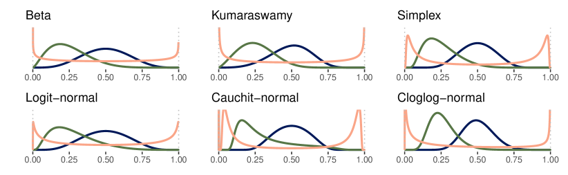
Without loss of generality, any double-bounded response $y$ with bounds $a,b$ can be linearly transformed to the unit interval by the transformation $f(y)=\frac{y-a}{b-a}$. Accordingly, it is sufficient to focus on likelihoods for unit interval data. We included the beta (Espinheira et al., 2008), Kumaraswamy (Kumaraswamy, 1980), simplex (Barndorff-Nielsen and Jørgensen, 1991), and transformed-normal (Atchison and Shen, 1980; Kim et al., 2017) likelihoods. The transformed-normal likelihoods arise from applying the link functions to the response variable $y$ (e.g., resulting in the logit-normal likelihood) instead of the location parameter $\mu$ as usual in standard GLMs. All of these likelihoods have two distributional parameters, one location (mean or median) and one scale (aka. shape) parameter. Figure 1 shows prototypical densities for each likelihood, illustrating qualitatively different shapes they can accommodate. The three distinct shapes are unimodal symmetric and asymmetric shapes as well as a bimodal (aka. bathtub) shape. As link functions, we included the logit, cloglog, and cauchit links, each of them having qualitatively different properties (Yin et al., 2020; Jiang et al., 2013; Lemonte and Bazán, 2018; Damisa et al., 2017; Fahrmeir et al., 1994; Gill et al., 2001; Powers and Xie, 2008; Morgan and Smith, 1992; Koenker and Yoon, 2009; Lemonte and Bazán, 2018). The logit link is based on the symmetric, light-tailed logistic distribution, the cloglog link is based on the asymmetric Gumbel distribution, while the cauchit link is based on the symmetric, heavy-tailed Cauchy distribution. Since logit and probit yield almost indistinguishable results due to the similar shapes of the logistic and the normal distributions (Fahrmeir et al., 1994; Gill et al., 2001; Powers and Xie, 2008), we decided against including the probit link despite its prominence.

Figure 1: Example illustrations of all included double-bounded densities each with three different shapes. The y-axis is truncated at 5 from above for better visibility of the different shapes.

3.1.2 Likelihoods and links for lower-bounded responses

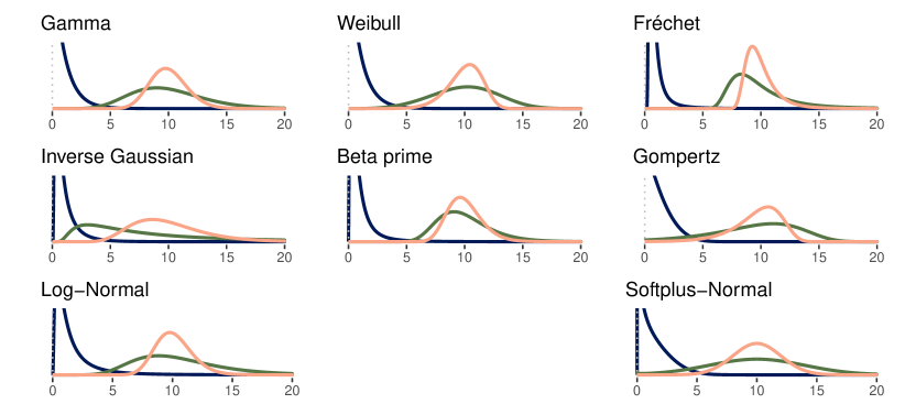
Without loss of generality, any continuous response $y$ with lower bound $a$ can be linearly transformed to have a lower bound of zero by the transformation $f(y)=y-a$. Accordingly, it is sufficient to focus on likelihoods for strictly positive data. We included the gamma, Weibull, Fréchet, beta prime, Gompertz, and transformed-normal likelihoods all of which have two distributional parameters, namely location (mean or median) and scale or shape. Figure 2 shows example densities for each likelihood, illustrating qualitatively different kinds of shapes they can accommodate. The three distinct shapes are unimodal thin tail and heavy tail shapes as well as a ramp shape. As link functions, we included the log and the softplus link. In contrast to the multiplicative log link, softplus approaches the identity for larger values, thus approximating additive behavior of regression terms while enforcing positive predictions (Zheng et al., 2015; Dugas et al., 2000).

Figure 2: Example illustrations of all included lower-bounded densities, each with three different shapes. The y-axis is truncated at 0.4 from above for better visibility of the different shapes.

3.1.3 Linear regression

In a nutshell, there are two kinds of approaches to choosing a likelihood. The first is to search within the space of structurally faithful (Bürkner et al., 2022a) likelihoods that respect the variable type of $y$, for example, an exponential or Gamma likelihood for positive continuous data that has no or no known upper bound. The second approach is just using a normal likelihood with identity link (i.e., linear regression) regardless of response type. The latter approach is openly advocated for comparably rarely (Hellevik, 2009) but de-facto applied across many disciplines because of its convenience and interpretability of the obtained regression coefficients. Still, there are obvious drawbacks of the "linear regression for all" approach. For instance, it can produce predictions that are impossible in reality (e.g., negative counts). What is more, it may drastically distort effect size estimates, their uncertainty, and sometimes even their sign in certain cases (Stroup, 2015; Martin and Williams, 2017; Williams and Martin, 2017; Liddell and Kruschke, 2018). To investigate this topic further, we also fit models using a normal likelihood and identity link in our simulations. Additionally, as an in-between approach between linear regression and structural faithful GLMs, we include the normal likelihood in combination with the appropriate (double- or lower-bounded) link functions.

3.2 Data Generation

Figure 3: Full data-generating graph. The ideal model is the subset of the full model that optimally estimates $\beta_{xy}$. Misspecifying with respect to each of the $z_{n}$ variables leads to four additional models, where excluding $z_{1}$ or including $z_{4}$ increases bias, while excluding $z_{2}$ or including $z_{3}$ increases variance of the estimation. As we don’t want estimation bias caused by causal misspecification in our models, we only include models misspecifying $z_{2}$ and $z_{3}$.

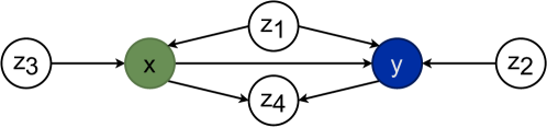
For each of the combinations of likelihood family, likelihood shape, and link presented in Section 3.1, we simulated data sets based on a single, prototypical causal directed acyclic graph (DAG; Pearl, 2009). The full DAG, shown in Figure 3, consists of an outcome $y$, a treatment $x$, and four additional variables $z_{1},z_{2},z_{3},z_{4}$ that correspond to four common, qualitatively different types of controls (Cinelli et al., 2020). With respect to the effect of $x$ on $y$, $z_{1}$ is a fork, $z_{2}$ is an ancestor of $y$, $z_{3}$ is an ancestor of $x$, and $z_{4}$ is a collider. These archetypes, plus the pipe $(x\rightarrow z\rightarrow y)$ that behaves like a fork, represent the majority of controls occurring in reality (Cinelli et al., 2020). We then used the following model to simulate the data sets:

$$z_{1} \sim\mathrm{normal}(0,\sigma_{z_{1}}),\quad z_{2}\sim\mathrm{normal}(0,\sigma_{z_{2}}),\quad z_{3}\sim\mathrm{normal}(0,\sigma_{z_{3}})$$

$$x \sim\mathrm{normal}(\beta_{z_{1}x}z_{1}+\beta_{z_{3}x}z_{3},\sigma_{x})$$

$$y \sim\textrm{likelihood}(\text{inv\_link}(\alpha_{y}+\beta_{xy}x+\beta_{z_{1}y}z_{1}+\beta_{z_{2}y}z_{2}),\phi)$$

$$z_{4} \sim\mathrm{normal}(\beta_{xz_{4}}x+\beta_{yz_{4}}y,\sigma_{z_{4}}).$$

Here, $\phi$ denotes the second distributional (scale or shape) parameter of the specified likelihood family and inv_link denotes the inverse link (aka response) function. We chose normal distributions to generate all data variables except for $y$ to control the scope of our simulations. Each simulated data set contained $100$ observations. Since the fitted models only have between 4 and 6 parameters, they are simple enough to be well identified on the basis of $100$ observations alone. A general challenge for Bayesian simulations that use prior distributions over parameters is the tendency to produce extreme data sets (Gabry et al., 2019; Mikkola et al., 2021). Additionally, the uncertainty propagation from the prior can blur the distinctiveness of the different likelihood shapes. To preserve control over the true DGP and to allow to control for the likelihood shapes during analysis, the parameters of the true DGP were thus set to fixed values, rather than being drawn from a prior distribution (Talts et al., 2018). Each likelihood’s second distributional parameter $\phi$ as well as the intercept $\alpha_{y}$ were chosen to produce the likelihood shapes presented in Section 3.1. The individual coefficients for $x$ and the $z_{i}$ were calibrated so that the parameter recovery was imperfect for the ideal model while also preventing the causally misspecified models from consistently failing (see also Section 3.3). The true causal effect $\beta_{xy}$ of $x$ on $y$ was either fixed to zero or set to a non-zero value that was calibrated together with all other coefficients. To prevent response values from under- or overflowing to the lower- or upper boundaries numerically, we truncated them near the boundaries with a tolerable error bound of $\varepsilon=10^{-6}$.

For each data generation configuration implied by fully crossing the design factors (see Table 1), we generated $200$ data sets, which resulted in $14,400$ data sets each for the double- and single-bounded scenarios.

Table 1: Overview of data generation configurations.

Factor	Levels
Double-bounded likelihoods	beta, Kumaraswamy, simplex, transformed-normal
Double-bounded links	logit, cauchit, cloglog
Double-bounded likelihood shapes	symmetric, asymmetric, bathtub
Lower-bounded likelihoods	gamma, Weibull, transformed-normal, Fréchet, beta-prime, Gompertz
Lower-bounded links	log, softplus
Lower-bounded likelihood shapes	ramp, heavy tail, thin tail
True $\beta_{xy}$	zero, positive

3.3 Model Fitting

On each simulated data set, we fitted all models resulting from the fully crossed combination of likelihoods and links (see Section 3.1) as well as a model with a normal likelihood and identity link to serve as a baseline (see Section 3.1.3). We then fit each resulting combination of likelihood and link with the three causally unbiased linear predictor terms implied by the DGP from Section 3.2 (see Table 2). Here, we only include causally misspecified models that don’t asymptotically bias the estimation of $\beta_{xy}$, as we are not investigating causal bias in this study. Thus remain the wrongful exclusion of $z_{2}$ or inclusion of $z_{3}$ to the ideal model, both increasing posterior variance (reducing precision) (Cinelli et al., 2020). In reference to R formula syntax, we will also use the term ’formulas’ to refer to the various linear predictor terms in the following. An overview of the model fit configurations is given in Table 2.

The fully-crossed design results in $48$ fit configurations for the double-bounded models and $45$ fit configurations for the lower-bounded models. Multiplied with $14400$ data sets each, this leads to a total of $691200$ double-bounded models and $648000$ single-bounded models, for a total of $1296000$ models fitted in our simulations.

Table 2: Overview of model fit configurations.

Factor	Levels
Double-bounded Likelihoods	beta, Kumaraswamy, simplex, transformed-normal, normal
Double-bounded Links	logit, cauchit, cloglog, identity (only with normal)
Single-bounded Likelihoods	gamma, Weibull, transformed-normal, Fréchet, beta-prime, Gompertz, normal
Single-bounded Links	log, softplus, identity (only with normal
Formulas (right-hand side)	$x+z_{1}+z_{2}$, $\;x+z_{1}$, $\;x+z_{1}+z_{2}+z_{3}$

Contrary to what we would recommend in practical applications of Bayesian models, we used flat priors for all model parameters, as it is not clear to us how one would specify equivalent priors for the different auxiliary parameters $\phi$ across all considered likelihoods. What is more, different links imply different latent scales, which render the regression coefficients’ scales incomparable across (assumed) links and thus further complicate equivalent prior specification. In a real-world analysis, we would prefer to use at least weakly-informative priors (Team, 2022; Gelman et al., 2013; McElreath, 2020). In pilot experiments (not reported here), we have confirmed that the differences in posteriors as well as the implied prediction metrics between models with flat vs. weakly informative priors are minimal for the models under investigation. We argue that such minimal differences do not justify extensive evaluation of different prior choices, since this is not the focus of the present paper. Additionally, the use of flat priors results in model estimations very similar to maximum likelihood estimation, which is why we expect the results of this study to generalize to frequentist models as well.

All models were fitted using Stan (Carpenter et al., 2017; Team, 2022) via brms (Bürkner, 2017) with two chains, 500 warmup- and 2000 post-warmup samples, which resulted in $4000$ total post-warmup posterior samples per model. We used an initialization range of $0.1$ around the origin on the unconstrained parameter space to avoid occasional initialization failures. For all other MCMC hyperparameters, we applied the brms defaults (Bürkner, 2017).

3.4 Model-Based Metrics

To measure parameter recovery of each fitted model, we used multiple metrics as detailed below. Implementations of these metrics are provided in the R packages posterior (Bürkner et al., 2022b), bayesim (Scholz et al., 2022a), and bayeshear (Scholz and Bürkner, 2022).

We calculated the posterior bias and $\mathrm{RMSE}$ of the model’s estimation of $\beta_{xy}$. Given a true parameter value $\theta^{\star}$ and a set of $S$ corresponding posterior samples $\{\theta^{(s)}\}:=\{\theta^{(s)}\}_{s=1}^{S}$, we compute the sampling-based posterior bias and $\mathrm{RMSE}$ as

$$\mathrm{bias}(\theta):=\mathrm{bias}(\{\theta^{(s)}\},\theta^{\star}):=\frac{1}{S}\sum^{S}_{s=1}\left(\theta^{(s)}\right)-\theta^{\star},$$ (3)

$$\mathrm{RMSE}(\theta):=\mathrm{RMSE}(\{\theta^{(s)}\},\theta^{\star}):=\sqrt{\frac{1}{S}\sum^{S}_{s=1}\left(\theta^{(s)}-\theta^{\star}\right)^{2}}=\sqrt{\mathrm{bias}(\theta)^{2}+\mathrm{Var}\left(\theta\right)},$$ (4)

where $\mathrm{Var}(\theta):=\mathrm{Var}(\{\theta^{(s)}\})$ denotes the variance over the posterior samples. Our analysis focuses on the true effect $\beta_{xy}$ and hence all metrics were computed for $\theta=\beta_{xy}$. Furthermore, as we are interested in the magnitude of the bias but not in its direction, we use the absolute bias in our results.

The above are reasonable measures for comparing models only if the assumed link coincides with the true link of the DGP. This is because the link determines the scale of the linear predictor and thus the comparability of the posterior samples $\{\beta_{xy}^{(s)}\}$ with the true parameter value $\beta^{\star}_{xy}$. To enable a comparison of models using different links, we also calculated the false positive rate (FPR; i.e., Type I-error rate) and the true positive rate (TPR; i.e., statistical power; inverse of the Type II-error rate) implied by the central 95% credible interval of $\{\beta_{xy}^{(s)}\}$. Significant CIs (no zero-overlap) count as true-positives in the case of non-zero true coefficients and false-positives in the case of a true coefficient of zero. These metrics can be inferred from our simulations, because the true effect $\beta_{xy}$ was set to zero in some conditions (to study FPR) and to non-zero values in others (to study TPR). In addition, we also present FPR and TPR in their combined form via receiver operating characteristic (ROC) curves (Zweig and Campbell, 1993) and the area under the ROC curve (AUC) (Bradley, 1997).

4 Results

Below, for brevity, we focus on a subset of results from our simulations that represent the main overarching patterns we observed. For example, the results for $|\mathrm{bias}(\beta_{xy})|$ generally showed the same patterns as those for $\mathrm{RMSE}(\beta_{xy})$, such that we only present the latter here. The complete results are available in our online appendix (Scholz and Bürkner, 2023b), together with the simulation data and code.

We excluded around 30000 models (2.3% of all models) from the analysis as they did not converge. Around 25,000 of the non-converged models were fit with a Fréchet likelihood and softplus link, a Gompertz likelihood, or a cloglog link, probably due to numerical instabilities. Specifically, we treated models as converged if the posterior samples $\{\beta_{xy}^{(s)}\}$ yielded $\widehat{R}<1.01$ and $\mathrm{ESS}>400$ (for details on these thresholds, see Vehtari et al. (2021)). Additionally, we required models to have less than $10$ divergent transitions out of a total of 4000 post-warmup iterations. While in practice, we would like all models to converge with no divergent transitions, this would have required extensive manual intervention to resolve all individual sampling problems, which is practically infeasible in our large simulation setup of more than one million models in total.

4.1 Double-bounded Results

Figure 4: $\mathrm{RMSE}(\beta_{xy})$ performance for the double-bounded scenarios split by data generating likelihood and shape for the logit link. Only models with fit link = data link are included. The point indicates the median, while the range spans the central 95% of the $\mathrm{RMSE}(\beta_{xy})$ values obtained in the simulations.

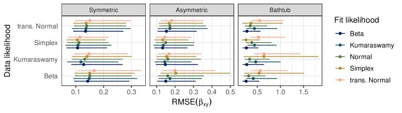
One of the most immediate observations is the stark difference between the bathtub shape on the one side and the symmetric and asymmetric likelihood shapes on the other side, as exemplarily shown in Figure 4 for the $\mathrm{RMSE}(\beta_{xy})$ and logit link. For both the symmetric and asymmetric likelihood shapes, the likelihood choice seems to have had little influence on $\mathrm{RMSE}(\beta_{xy})$ across all links. For the bathtub shape, the beta likelihood showed the best average $\mathrm{RMSE}(\beta_{xy})$. Depending on the scenario, the normal and Kumaraswamy likelihoods achieved similar performance but with less overall consistency. The differences between links and data generating likelihoods were minor. As the only exception, we found that the cauchit-normal likelihood models performed considerably worse than all others.

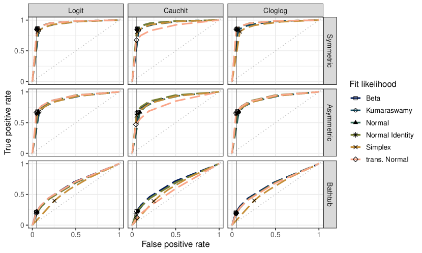
In terms of error rates and ROC averaged over DGP link and likelihood family, as shown in Figure 5, there are two noteworthy observations. First, likelihood choice again seems to have had little influence on calibration besides the worse performance of the cauchit-normal (middle column of Figure 5) and simplex (bottom row of Figure 5) likelihoods. This closely matches the patterns found for $\mathrm{RMSE}(\beta_{xy})$. Second, the normal-identity (linear regression) model had error rates similar to the well performing canonical likelihood and link combinations. The differences in error rates between data generating likelihoods and links as well as fit formulas were minor.

Figure 5: ROC for the double-bounded scenarios split by likelihood shape and fit links. The curves are calculated from the 50%, 80%, 90%, and 95% CIs, with the 95% CI highlighted with a different symbol per fit likelihood. The vertical line indicates the nominal 0.05 FPR of the 95% CI.

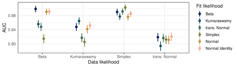
Finally, Figure 6 shows the conditional effects of the interaction of data and fit likelihood on the AUC. The results imply that the true likelihood family has the highest (median) AUC in each case, shortly followed by the normal likelihoods, both with the appropriate links and the identity link. Overall, we can observe very similar trends as with the other results, where differences are often small in absolute numbers. Depending on the application, the relative differences might however be relevant, as a false positive reduction from $0.05$ to $0.04$ would be a reduction of false-positives by $20\%$. The conditional effects of the fit links on the AUC (shown in the online appendix Scholz and Bürkner (2023b)) are very close to each other, with the logit link having the highest and the cauchit link having the lowest AUC for every data link.

Figure 6: Conditional effects of data and fit likelihood on the area under the ROC curve (AUC) for the double-bounded scenarios.

4.2 Lower-bounded Results

Figure 7: $\mathrm{RMSE}(\beta_{xy})$ performance for the lower-bounded scenarios split by data generating likelihood and shape for the log link. Only models with fit link = data link are included. The point indicates the median, while the range spans the central 95% of the $\mathrm{RMSE}(\beta_{xy})$ values obtained in the simulations. The x-axes are truncated for improved readability.

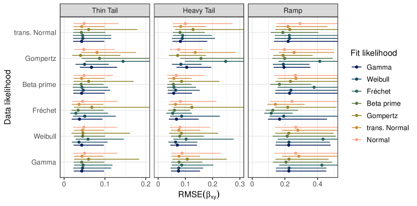
Similar to the double-bounded data simulations, one of the most immediate observations is the difference between likelihood shapes. Specifically, for the log link, the ramp shape led to higher $\mathrm{RMSE}(\beta_{xy})$ compared to other likelihood shapes (see Figure 7). In contrast, for the softplus link, the heavy tail shape implied the highest $\mathrm{RMSE}(\beta_{xy})$ (see the online appendix (Scholz and Bürkner, 2023b)). The differences between fit likelihoods were again small. Notable exceptions to those general trends were the worse RMSE for the beta prime likelihood on all Gompertz data and softplus-normal heavy-tailed data. In addition, both the normal and transformed-normal likelihoods had worse recovery for the ramp shape compared to the other shapes. The Gompertz and Fréchet likelihoods generally lacked consistency and had worse recovery than the other likelihoods outside of a few favourable scenarios.

In terms of error rates, we observed similar behaviour as for the double-bounded scenarios but with more variation between the fit likelihoods. Similar to the results for $\mathrm{RMSE}(\beta_{xy})$, the Gompertz and Fréchet likelihoods showed an increased FPR across all scenarios, with less consistency for the remaining likelihoods in each individual case. Similar to the double-bounded results, the normal-identity (linear regression) models had similar error rates to the well-performing but structurally faithful lower-bounded likelihood and link combinations.

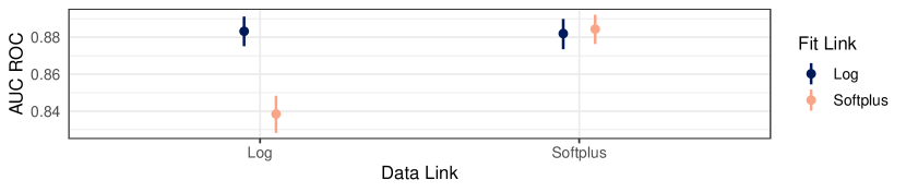
For the lower-bounded scenarios, the conditional effects of the interaction between data and fit likelihood (not shown here) exhibited fewer differences among fit families compared to the double-bounded results. Similar to the earlier results, the Fréchet and Gompertz distributions consistently had lower AUC as the others, while the differences between the latter were small. While the true likelihood family was always among the best performing ones, it is worth noting that it did not consistently yield a higher AUC than all alternative families. The conditional effects of the interaction of data and fit link (see Figure 8) illustrate that the log link had consistently high (average) AUC for both log and softplus data, while the softplus link showed substantially lower AUC specifically for log data. At this point the exact mechanism that causes this asymmetry remains unclear.

Figure 8: Conditional effects of data and fit link on the AUC for the lower-bounded scenarios.

5 Discussion

This paper aims to advance our understanding of how the misspecification of likelihood families and link functions influences posterior accuracy and calibration of (Bayesian) GLMs. In this section we discuss the simulation results presented in Section 4, collect potentially useful learnings for practical applications, and provide suggestions for future research. For brevity, we again use the term parameter recovery (PR) to refer to both posterior accuracy and calibration.

For both data types, we observed groups of well-behaving likelihoods that had similar PR. In both cases we also found a group of notably worse performing likelihoods, not only in terms of PR, but also in terms of sampling efficiency and convergence. Accordingly, at least within the considered scenarios, likelihood choice appears to have little influence, as long as one chooses any of the well-behaving likelihood families. Based on our results, we would advise practitioners to use a beta, Kumaraswamy or logit-normal likelihood for double-bounded data. The beta distribution consistently led to good PR across all DGPs, while the Kumaraswamy and logit-normal likelihoods were slightly less consistent but still generally well-behaving. For the lower-bounded data, we suggest the use of a log-normal, gamma, Weibull or beta prime likelihood. The log-normal likelihood showed the highest consistency and general good performance, with the gamma, Weibull and beta prime likelihoods again showing generally good performance but with less consistency. Additionally, the normal likelihood was among the best performing likelihoods both when using with the matching link functions, for both data-types. However, care has to be taken here, as the normal likelihood does not respect the boundaries of the outcome data, such that we would only recommend its use in cases where this poses no risk. The likelihoods that performed less consistently and overall worse generally had longer (fatter) tails, particularly the Fréchet and cauchit-normal likelihoods. That being said, the respective true likelihood had among the lowest average $\mathrm{RMSE}(\beta_{xy})$ and $|\mathrm{bias}(\beta_{xy})|$, as well as highest average AUC in all scenarios. The implication for practice is that one would still benefit from using the true likelihood, even if it were not part of the well-behaving group of likelihoods and PR is the main goal of the analysis. Section 5.1 provides some examples of approaches for finding a well-fitting likelihood.

In terms of link function choice, the double-bounded links all produced similar results, though we found the logit link to generally be more stable during sampling and more commonly supported in statistics software packages. Here, we see little benefit of using alternative links based on our results and practical experience. The lower-bounded links differed more strongly among each other, as the log link was clearly more robust than the softplus link. These patterns certainly depend on the specifically included likelihood families and link functions and are likely subject to change if other link functions were included. This would imply the log link as the default choice for any analysis, however, we would prefer to better understand the underlying mechanism before a full endorsement.

In addition, we found that models using a normal likelihood with an identity link (i.e., linear regression) had both similar false-positive and true-positive rates to the structurally faithful alternatives. This indicates that in practice, linear regression can be a valid alternative if frequentist calibration is the primary objective of an analysis, even when responses are bounded. This result is also reassuring for the validity of many scientific results more generally as it shows that the practice of using linear regression can have good calibration even if it is not structurally faithful. Additional relevance is provided by the fact that the estimation speed of linear regression models can be magnitudes faster than other GLMs, due do the availability of highly optimized implementations in both Bayesian and frequentist frameworks, an important aspect of especially Bayesian workflows, that often suffer from slow model fitting Gelman et al. (2020b); Bürkner et al. (2022a).

All of the above recommendations could be considered default options, i.e., they are already commonly used in reference and teaching materials and have good software support (McElreath, 2020; Gelman et al., 2013; Team, 2022). To reiterate, if one is interested in posterior accuracy, we would suggest the above default choices as long as there is no additional information, e.g., from model comparisons (Scholz and Bürkner, 2023a), that would support the use of a different likelihood or link: As exemplified by data generated from a simplex likelihood with bathtub shape, there definitely are cases where those default likelihoods (or links) wouldn’t be a good choice. If calibration is the main objective of a statistical analysis, however, our results suggests that linear regression is as reliable as the structurally faithful likelihood and link alternatives, while potentially offering greatly increased computational performance due to optimized implementations.

5.1 Future Work

To our knowledge, the present paper is one of the largest comparison studies of its type with a total of over one million fitted models. Still, there are almost surely relevant likelihoods or link functions used in some research fields that we have missed. A continuation of this work, focusing on the requirements of specific research fields could add valuable understanding in those areas. Similarly, an extension to other data domains, such as unbounded-continuous, count, or ordinal data, would also help to assess the generalizability of our results. This is especially relevant for the finding that linear regression (normal-identity) models achieve good error calibration across domains.

Finally, the use of a small set of likelihood shapes could have introduced a form of artificial similarity in the data generation process across likelihoods. This could both favour likelihoods that accompany said shapes more easily and reduce differences between likelihoods by forcing them into the same shapes. Future research in this direction could thus use a more general perspective on likelihood shapes, allowing to highlight differences among DGPs more clearly. One option could be to sample the auxiliary parameters responsible for the likelihood shape from appropriate prior distributions to increase the diversity of true likelihood shapes. Alternatively, one could use real data sets as the foundation of the data-generating process to more closely simulate problems encountered in practice.

Funding

This work was partially funded by the Deutsche Forschungsgemeinschaft (DFG, German Research Foundation) under Germany’s Excellence Strategy – EXC-2075 - 390740016 (the Stuttgart Cluster of Excellence SimTech).

This work was performed on the computational resource bwUniCluster funded by the Ministry of Science, Research and the Arts Baden-Württemberg and the Universities of the State of Baden-Württemberg, Germany, within the framework program bwHPC.

The authors gratefully acknowledge the support and funding.

Data availability

The data that support the findings of this study are openly available in OSF at http://doi.org/10.17605/OSF.IO/TMDCF.

References

- Gelman et al. [2020a] Andrew Gelman, Jennifer Hill, and Aki Vehtari. Regression and other stories. Cambridge University Press, 2020a.
- Harrell [2015] Frank E Harrell. Regression modeling strategies: with applications to linear models, logistic and ordinal regression, and survival analysis. Springer, 2015.
- Nelder and Wedderburn [1972] John Ashworth Nelder and Robert WM Wedderburn. Generalized linear models. Journal of the Royal Statistical Society: Series A (General), 135(3):370–384, 1972. Publisher: Wiley Online Library.
- Gill et al. [2001] Jeff Gill, Jefferson M Gill, Michelle Torres, and Silvia Michelle Torres Pacheco. Generalized linear models: a unified approach, volume 134. Sage Publications, 2001.
- Bates et al. [2015] Douglas Bates, Martin Mächler, Ben Bolker, and Steve Walker. Fitting Linear Mixed-Effects Models Using \pkglme4. Journal of Statistical Software, 67(1):1–48, 2015.
- Bürkner [2017] Paul-Christian Bürkner. brms: An r package for bayesian multilevel models using stan. Journal of statistical software, 80:1–28, 2017.
- McCullagh [2019] Peter McCullagh. Generalized linear models. Routledge, 2019.
- James et al. [2013] Gareth James, Daniela Witten, Trevor Hastie, and Robert Tibshirani. An introduction to statistical learning, volume 112. Springer, 2013.
- Gelman et al. [2013] Andrew Gelman, John B. Carlin, Hal S. Stern, David B. Dunson, Aki Vehtari, and Donald B. Rubin. Bayesian Data Analysis. Chapman and Hall/CRC, New York, 3 edition, July 2013. ISBN 978-0-429-11307-9. doi:10.1201/b16018.
- Gelman et al. [2017] Andrew Gelman, Daniel Simpson, and Michael Betancourt. The prior can often only be understood in the context of the likelihood. Entropy, 19(10):555–567, 2017. Publisher: Multidisciplinary Digital Publishing Institute.
- Gelman et al. [2020b] Andrew Gelman, Aki Vehtari, Daniel Simpson, Charles C. Margossian, Bob Carpenter, Yuling Yao, Lauren Kennedy, Jonah Gabry, Paul-Christian Bürkner, and Martin Modrák. Bayesian Workflow. arXiv:2011.01808 [stat], November 2020b. arXiv: 2011.01808.
- McElreath [2020] Richard McElreath. Statistical Rethinking: A Bayesian Course with Examples in R and Stan. Chapman and Hall/CRC, New York, 2 edition, March 2020. ISBN 978-0-429-02960-8. doi:10.1201/9780429029608.
- Huber et al. [1967] Peter J Huber et al. The behavior of maximum likelihood estimates under nonstandard conditions. In Proceedings of the fifth Berkeley symposium on mathematical statistics and probability, volume 1, pages 221–233. Berkeley, CA: University of California Press, 1967.
- Li and Duan [1989] Ker-Chau Li and Naihua Duan. Regression analysis under link violation. The Annals of Statistics, 17(3):1009–1052, 1989.
- Fahrmexr [1990] Ludwig Fahrmexr. Maximum likelihood estimation in misspecified generalized linear models. Statistics, 21(4):487–502, 1990.
- Fomby and Carter Hill [2003] Thomas B Fomby and R Carter Hill. Maximum likelihood estimation of misspecified models: twenty years later. Emerald Group Publishing Limited, 2003.
- White [1982] Halbert White. Maximum likelihood estimation of misspecified models. Econometrica: Journal of the econometric society, pages 1–25, 1982.
- Yu and Huang [2019] Shun Yu and Xianzheng Huang. Link misspecification in generalized linear mixed models with a random intercept for binary responses. Test, 28(3):827–843, 2019.
- Huang [2021] Xianzheng Huang. Improved wrong-model inference for generalized linear models for binary responses in the presence of link misspecification. Statistical Methods & Applications, 30(2):437–459, 2021.
- Chen et al. [2018] Wansu Chen, Lei Qian, Jiaxiao Shi, and Meredith Franklin. Comparing performance between log-binomial and robust poisson regression models for estimating risk ratios under model misspecification. BMC medical research methodology, 18(1):1–12, 2018.
- Czado and Santner [1992] Claudia Czado and Thomas J Santner. The effect of link misspecification on binary regression inference. Journal of statistical planning and inference, 33(2):213–231, 1992.
- Cangul et al. [2009] MZ Cangul, Yves Rene Chretien, R Gutman, and Donald B Rubin. Testing treatment effects in unconfounded studies under model misspecification: Logistic regression, discretization, and their combination. Statistics in medicine, 28(20):2531–2551, 2009.
- Dongen and Møller [2007] Stefan Van Dongen and Anders Pape Møller. On the distribution of developmental errors: comparing the normal, gamma, and log-normal distribution. Biological Journal of The Linnean Society, 92:197–210, 2007.
- Jacqmin-Gadda et al. [2007] Hélène Jacqmin-Gadda, Solenne Sibillot, Cécile Proust, Jean-Michel Molina, and Rodolphe Thiébaut. Robustness of the linear mixed model to misspecified error distribution. Computational Statistics & Data Analysis, 51(10):5142–5154, 2007.
- Dumonceaux and Antle [1973] Robert Dumonceaux and Charles E Antle. Discrimination between the log-normal and the weibull distributions. Technometrics, 15(4):923–926, 1973.
- Gupta and Kundu [2003] Rameshwar D. Gupta and Debasis Kundu. Discriminating between weibull and generalized exponential distributions. Comput. Stat. Data Anal., 43:179–196, 2003.
- Vuong [1989] Quang H Vuong. Likelihood ratio tests for model selection and non-nested hypotheses. Econometrica: journal of the Econometric Society, pages 307–333, 1989.
- Lewis et al. [2011] Fraser Lewis, Adam Butler, and Lucy Gilbert. A unified approach to model selection using the likelihood ratio test. Methods in ecology and evolution, 2(2):155–162, 2011.
- Dick [2004] EJ Dick. Beyond ‘lognormal versus gamma’: discrimination among error distributions for generalized linear models. Fisheries Research, 70(2-3):351–366, 2004.
- Ward [2008] Eric J Ward. A review and comparison of four commonly used bayesian and maximum likelihood model selection tools. Ecological Modelling, 211(1-2):1–10, 2008.
- Kundu and Manglick [2004] Debasis Kundu and Anubhav Manglick. Discriminating between the weibull and log-normal distributions. Naval Research Logistics (NRL), 51(6):893–905, 2004.
- Barreto-Souza and Silva [2015] Wagner Barreto-Souza and Rodrigo B Silva. A likelihood ratio test to discriminate exponential–poisson and gamma distributions. Journal of Statistical Computation and Simulation, 85(4):802–823, 2015.
- Dey and Kundu [2009] Arabin Kumar Dey and Debasis Kundu. Discriminating among the log-normal, weibull, and generalized exponential distributions. IEEE Transactions on reliability, 58(3):416–424, 2009.
- Bürkner et al. [2022a] Paul-Christian Bürkner, Maximilian Scholz, and Stefan T. Radev. What makes a good bayesian model? towards a unified model taxonomy. arXiv preprint, 2022a.
- Scholz and Bürkner [2023a] Maximilian Scholz and Paul-Christian Bürkner. Prediction can be safely used as a proxy for explanation in causally consistent bayesian generalized linear models, 2023a.
- R Core Team [2018] R Core Team. R: A Language and Environment for Statistical Computing. R Foundation for Statistical Computing, Vienna, Austria, 2018. URL https://www.R-project.org/.
- Team [2022] Stan Development Team. Stan modeling language users guide and reference manual, 2.30.0, 2022. URL https://mc-stan.org.
- Carpenter et al. [2017] Bob Carpenter, Andrew Gelman, Matthew D Hoffman, Daniel Lee, Ben Goodrich, Michael Betancourt, Marcus Brubaker, Jiqiang Guo, Peter Li, and Allen Riddell. Stan: A probabilistic programming language. Journal of statistical software, 76(1), 2017.
- Scholz et al. [2022a] Maximilian Scholz, Yannick Dzubba, and Paul-Christian Bürkner. Bayesim, Sep 2022a. URL https://github.com/sims1253/bayesim. R package version 0.29.5.9000.
- Scholz et al. [2022b] Maximilian Scholz, Yannick Dzubba, and Paul-Christian Bürkner. bayesfam: Custom families for brms, 2022b. URL https://github.com/sims1253/bayesfam. R package version 0.2.4.
- Scholz and Bürkner [2022] Maximilian Scholz and Paul-Christian Bürkner. bayeshear: Toolbox of bayesian model metrics, 2022. URL https://github.com/sims1253/bayeshear. R package version 0.2.0.9000.
- Scholz and Bürkner [2023b] Maximilian Scholz and Paul-Christian Bürkner. Posterior accuracy and calibration under misspecification in bayesian generalized linear models: Online appendix, September 2023b. URL https://osf.io/tmdcf/.
- Johnson et al. [1995] Norman L. Johnson, Samuel Kotz, and Narayanaswamy Balakrishnan. Continuous Univariate Distributions, Volume 2. John Wiley & Sons, May 1995. ISBN 978-0-471-58494-0.
- Johnson et al. [2005] Norman L Johnson, Samuel Kotz, and Adrienne W Kemp. Univariate discrete distributions. John Wiley & Sons, 2005.
- Stasinopoulos and Rigby [2007] D Mikis Stasinopoulos and Robert A Rigby. Generalized additive models for location scale and shape (GAMLSS) in R. Journal of Statistical Software, 23(7):1–46, 2007.
- Yee [2010] Thomas W Yee. The VGAM package for categorical data analysis. Journal of Statistical Software, 32(10):1–34, 2010. Publisher: Citeseer.
- Bürkner [2021] Paul-Christian Bürkner. Bayesian Item Response Modelling in R with brms and Stan. Journal of Statistical Software, pages 1–54, 2021.
- Espinheira et al. [2008] Patrícia L Espinheira, Silvia LP Ferrari, and Francisco Cribari-Neto. On beta regression residuals. Journal of Applied Statistics, 35(4):407–419, 2008.
- Kumaraswamy [1980] P. Kumaraswamy. A generalized probability density function for double-bounded random processes. Journal of Hydrology, 46(1):79–88, March 1980. ISSN 0022-1694. doi:10.1016/0022-1694(80)90036-0.
- Barndorff-Nielsen and Jørgensen [1991] O. E. Barndorff-Nielsen and B. Jørgensen. Some parametric models on the simplex. Journal of Multivariate Analysis, 39(1):106–116, October 1991. ISSN 0047-259X. doi:10.1016/0047-259X(91)90008-P.
- Atchison and Shen [1980] J. Atchison and S.M. Shen. Logistic-normal distributions: Some properties and uses. Biometrika, 67(2):261–272, January 1980. ISSN 0006-3444. doi:10.1093/biomet/67.2.261.
- Kim et al. [2017] Seongho Kim, Elisabeth Heath, and Lance Heilbrun. Sample size determination for logistic regression on a logit-normal distribution. Statistical Methods in Medical Research, 26(3):1237–1247, June 2017. ISSN 0962-2802. doi:10.1177/0962280215572407. Publisher: SAGE Publications Ltd STM.
- Yin et al. [2020] Shuang Yin, Dipak K. Dey, Emiliano A. Valdez, Guojun Gan, and Jeyaraj Vadiveloo. Skewed link regression models for imbalanced binary response with applications to life insurance. arXiv:2007.15172 [stat], July 2020.
- Jiang et al. [2013] Xun Jiang, Dipak K. Dey, Rachel Prunier, Adam M. Wilson, and Kent E. Holsinger. A new class of flexible link functions with application to species co-occurrence in cape floristic region. The Annals of Applied Statistics, 7(4):2180–2204, 2013. ISSN 1932-6157.
- Lemonte and Bazán [2018] Artur J. Lemonte and Jorge L. Bazán. New links for binary regression: an application to coca cultivation in Peru. TEST, 27(3):597–617, September 2018. ISSN 1133-0686, 1863-8260. doi:10.1007/s11749-017-0563-1.
- Damisa et al. [2017] S Damisa, F Musa, and S Sani. On the comparison of some link functions in binary response analysis. Biomedical Statistics and Informatics, 2(4):145–149, 2017.
- Fahrmeir et al. [1994] Ludwig Fahrmeir, Gerhard Tutz, Wolfgang Hennevogl, and Eliane Salem. Multivariate statistical modelling based on generalized linear models, volume 425. Springer, 1994.
- Powers and Xie [2008] Daniel Powers and Yu Xie. Statistical methods for categorical data analysis. Emerald Group Publishing, 2008.
- Morgan and Smith [1992] Byron JT Morgan and DM Smith. A note on Wadley’s problem with overdispersion. Journal of the Royal Statistical Society: Series C (Applied Statistics), 41(2):349–354, 1992. Publisher: Wiley Online Library.
- Koenker and Yoon [2009] Roger Koenker and Jungmo Yoon. Parametric links for binary choice models: A Fisherian–Bayesian colloquy. Journal of Econometrics, 152(2):120–130, October 2009. ISSN 0304-4076. doi:10.1016/j.jeconom.2009.01.009.
- Zheng et al. [2015] Hao Zheng, Zhanlei Yang, Wenju Liu, Jizhong Liang, and Yanpeng Li. Improving deep neural networks using softplus units. In 2015 International joint conference on neural networks (IJCNN), pages 1–4. IEEE, 2015.
- Dugas et al. [2000] Charles Dugas, Yoshua Bengio, François Bélisle, Claude Nadeau, and René Garcia. Incorporating second-order functional knowledge for better option pricing. Advances in neural information processing systems, 13, 2000.
- Hellevik [2009] Ottar Hellevik. Linear versus logistic regression when the dependent variable is a dichotomy. Quality & Quantity, 43(1):59–74, January 2009. ISSN 0033-5177, 1573-7845. doi:10.1007/s11135-007-9077-3.
- Stroup [2015] Walter W Stroup. Rethinking the analysis of non-normal data in plant and soil science. Agronomy journal, 107(2):811–827, 2015.
- Martin and Williams [2017] Stephen R Martin and Donald R Williams. Outgrowing the procrustean bed of normality: the utility of Bayesian modeling for asymmetrical data analysis. PsyArXiv preprint, 2017.
- Williams and Martin [2017] Donald R Williams and Stephen R Martin. Rethinking robust statistics with modern Bayesian methods. PsyArXiv preprint, 2017.
- Liddell and Kruschke [2018] Torrin M Liddell and John K Kruschke. Analyzing ordinal data with metric models: What could possibly go wrong? Journal of Experimental Social Psychology, 79:328–348, 2018. Publisher: Elsevier.
- Pearl [2009] Judea Pearl. Causality. Cambridge university press, 2009.
- Cinelli et al. [2020] Carlos Cinelli, Andrew Forney, and Judea Pearl. A Crash Course in Good and Bad Controls. SSRN Electronic Journal, 2020. ISSN 1556-5068. doi:10.2139/ssrn.3689437.
- Gabry et al. [2019] Jonah Gabry, Daniel Simpson, Aki Vehtari, Michael Betancourt, and Andrew Gelman. Visualization in Bayesian workflow. Journal of the Royal Statistical Society: Series A (Statistics in Society), 182(2):389–402, February 2019. ISSN 09641998. doi:10.1111/rssa.12378.
- Mikkola et al. [2021] Petrus Mikkola, Osvaldo A Martin, Suyog Chandramouli, Marcelo Hartmann, Oriol Abril Pla, Owen Thomas, Henri Pesonen, Jukka Corander, Aki Vehtari, Samuel Kaski, Bürkner, Paul-Christian, and Klami, Arto. Prior knowledge elicitation: The past, present, and future. arXiv preprint arXiv:2112.01380, 2021.
- Talts et al. [2018] Sean Talts, Michael Betancourt, Daniel Simpson, Aki Vehtari, and Andrew Gelman. Validating bayesian inference algorithms with simulation-based calibration. arXiv preprint arXiv:1804.06788, 2018.
- Bürkner et al. [2022b] Paul-Christian Bürkner, Jonah Gabry, Matthew Kay, and Aki Vehtari. posterior: Tools for working with posterior distributions, 2022b. URL https://mc-stan.org/posterior/. R package version 1.3.0.
- Zweig and Campbell [1993] Mark H Zweig and Gregory Campbell. Receiver-operating characteristic (roc) plots: a fundamental evaluation tool in clinical medicine. Clinical chemistry, 39(4):561–577, 1993.
- Bradley [1997] Andrew P Bradley. The use of the area under the roc curve in the evaluation of machine learning algorithms. Pattern recognition, 30(7):1145–1159, 1997.
- Vehtari et al. [2021] Aki Vehtari, Andrew Gelman, Daniel Simpson, Bob Carpenter, and Paul-Christian Bürkner. Rank-normalization, folding, and localization: An improved $\widehat{R}$ for assessing convergence of MCMC. Bayesian Analysis, 16(2), June 2021. ISSN 1936-0975. doi:10.1214/20-BA1221. arXiv: 1903.08008.