Edge Accelerated Robot Navigation with
Hierarchical Motion Planning

Abstract

Low-cost autonomous robots suffer from limited onboard computing power, resulting in excessive computation time when navigating in cluttered environments. This paper presents Edge Accelerated Robot Navigation, or EARN for short, to achieve real-time collision avoidance by adopting hierarchical motion planning (HMP). In contrast to existing local or edge motion planning solutions that ignore the inter-dependency between low-level motion planning and high-level resource allocation, EARN adopts model predictive switching (MPS) that maximizes the expected switching gain w.r.t. robot states and actions under computation and communication resource constraints. As such, each robot can dynamically switch between a point-mass motion planner executed locally to guarantee safety (e.g., path-following) and a full-shape motion planner executed non-locally to guarantee efficiency (e.g., overtaking). The crux to EARN is a two-time scale integrated decision-planning algorithm based on bilevel mixed-integer optimization, and a fast conditional collision avoidance algorithm based on penalty dual decomposition. We validate the performance of EARN in indoor simulation, outdoor simulation, and real-world environments. Experiments show that EARN achieves significantly smaller navigation time and collision ratios than state-of-the-art navigation approaches.

I Introduction

Navigation is a fundamental task for mobile robots, which determines a sequence of control commands to move the robot from its current state to a target state without any collision [1]. The navigation time and collision ratio critically depend on how fast the robot can compute a trajectory. The computation time is proportional to the size of state space, which is mainly determined by the number of obstacles (spatial) and the length of prediction horizon (temporal) [2]. In cluttered environments with numerous obstacles, the shape of obstacles should also be considered, and the computation time is further multiplied by the number of planes for each obstacle [3]. Therefore, navigation is challenging for low-cost robots in cluttered environments.

Currently, most existing approaches reduce the computation time from an algorithm design perspective, e.g., using heuristics [4], approximations [5], parallelizations [6, 7, 8, 9], or learning [10, 11, 12] techniques. This paper accelerates the robot navigation from an integrated networking and algorithm design perspective, i.e., the robot can opportunistically execute advanced navigation algorithms by accessing a proximal edge computing server [13, 14, 15]. In this way, low-cost robots can accomplish collision avoidance and aggressive overtaking in cluttered environments.

However, design and implementation of edge-assisted navigation is non-trivial. First, it involves periodic data exchange between robots and servers, meaning that the server should have low-latency access to the robot; otherwise, communication delays may lead to collisions. Second, different robots may compete for computing resources and robot selection is needed to avoid resource squeeze. Third, the computation time of multi-robot full-shape navigation may become unacceptable even at the server, calling for parallel optimizations. Finally, in case of no proximal server, the robots should be able to navigate locally and individually by switching to local conservative planning algorithms. All these observations imply that edge-assisted navigation needs to maximize the navigation efficiency under practical resource constraints, for which the existing local [6, 7, 8, 9] or edge [13, 14, 15] planning methods become inefficient and unsafe, as they ignore the interdependence between low-level motion planning (e.g., robot states and actions) and high-level decision-making (e.g., planner switching and resource management).

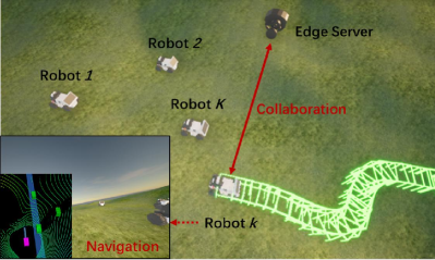
Figure 1: Four low-cost robots execute full-shape collision avoidance assisted by a proximal edge server based on EARN.

This paper proposes Edge Accelerated Robot Navigation (EARN) as shown in Fig. 1, which is a hierarchical motion planning (HMP) framework that enables smooth switching between a local motion planner at the robot and an edge motion planner at the server. This is realized through tightly-coupled decision-making and motion planning (T-DMMP), which solves a newly derived model predictive switching (MPS) problem. The MPS maximizes the expected switching gain under computation and communication resource constraints, which is in contrast to existing model predictive control (MPC) where robot states and actions are the only considerations. In particular, for the high-level resource management, a planning-aware decision-making algorithm is devised based on bilevel mixed-integer nonlinear programming (B-MINLP), which can automatically identify robots navigating in complex environments while orchestrating computation and communication resources. For the low-level motion planning, we incorporate a conditional collision avoidance constraint and propose a penalty dual decomposition (PDD) algorithm, which computes collision-free trajectories in a convergence-guaranteed parallel manner. We implement our methods by Robot Operation System (ROS) and validate them in the high-fidelity Car-Learning-to-Act (CARLA) simulation. Experiments confirm the superiority of the proposed scheme compared with various benchmarks such as Path Following (PF) [4] and Earliest Deadline First (EDF) [16] in both indoor and outdoor scenarios. We also implement EARN in a multi-robot testbed, where real-world experiments are conducted to demonstrate the practical applicability of EARN. Our codes will be released as open-source ROS packages.

The contribution of this paper is summarized as follows:

• Propose a T-DMMP framework based on MPS, which enables smooth planner switching in dynamic environments under resource constraints.

• Propose a PDD algorithm, which guarantees convergence for parallelization and ensures real-time navigation.

• Implementation of EARN in both simulation and real-world environments and extensive evaluations of the performance gain brought by EARN.

The remainder of the paper is organized as follows. Section II reviews the related work. Section III presents the architecture and mechanism of the proposed EARN. Section IV presents the core optimization algorithms for EARN. Simulations and experiments are demonstrated and analyzed in Section V. Finally, conclusion is drawn in Section VI.

II Related Work

Motion Planning is a challenge when navigating low-cost robots, due to contradiction between the stringent timeliness constraint and the limited onboard computing capability. Current motion planning can be categorized into heuristic based and optimization based. Heuristic methods (e.g., path following [4], spatial cognition [17]) are over-conservative, and the robot may get stuck in cluttered environments. On the other hand, optimization based techniques can overcome this issue by explicitly formulating collision avoidance as distance constraints. Model predictive control (MPC) [3, 4, 2, 6, 7, 8, 9] is the most widely used optimization algorithm, which builds the relation between future states and current states based on vehicle and obstacle dynamics, and leverages constrained optimization for generating collision-free trajectories in complex scenarios. Nonetheless, MPC could be time-consuming when the number of obstacles is large.

Optimization Based Collision Avoidance can be accelerated in two ways. First, imitation learning methods [10, 11, 12] can learn from optimization solvers’ demonstrations using deep neural networks. As such, iterative optimization is transformed into a feed-forward procedure that can generate driving signals in milliseconds. However, learning-based methods may break down if the target scenario contains examples outside the distribution of the training dataset [12]. Second, the computation time can be reduced by parallel optimizations [6, 7, 8, 9]. For instance, the alternating direction method of multipliers (ADMM) has been adopted in multi-robot navigation systems [9], which decomposes a large centralized problem into several subproblems that are solved in parallel for each robot. By applying parallel computation to obstacle avoidance, ADMM has been shown to accelerate autonomous navigation in cluttered environments [8]. However, ADMM is not guaranteed to converge when solving nonconvex problems [18]. Unfortunately, motion planning problems are nonconvex due to the nonlinear vehicle dynamics and non-point-mass obstacle shapes [3, 8]. Here, we develop a PDD planner that converges to a Karush-Kuhn-Tucker (KKT) solution and overcomes the occasional failures of ADMM.

Cloud, Fog, Edge Robotics are emerging paradigms to accelerate robot navigation [13]. The idea is to allow robots to access proximal computing resources. For example, robot inference and learning applications, such as object recognition and grasp planning, can be offloaded to cloud, edge, and fog as a service [14]. Edge-assisted autonomous driving was investigated in [16], which offloads the heavy tasks from low-cost vehicular computers to powerful edge servers. However, this type of approach would introduce additional communication latency [19]. To reduce the communication latency, a partial offloading scheme was proposed for vision-based robot navigation [15]. A priority-aware robot scheduler was proposed to scale up collaborative visual SLAM service in edge offloading settings [20]. A cloud robotics platform FogROS2 was proposed to effectively connect robot systems across different physical locations, networks, and data distribution services [21]. Nonetheless, current cloud and edge robotics schemes ignore the interdependence between the low-level motion planning (e.g., robot states and actions) and the high-level decision-making (e.g., planner switching and resource management).

This paper proposes a T-DMMP framework through the two time-scale bilevel optimization formulation. For the higher-level subproblem, the beneficial robot is selected according to the resource constraint and the switching gain, which is a difference-of-norm function w.r.t the low-level robot trajectories and actions. On the other hand, for the lower-level subproblem, a hierarchical motion planning problem is formulated by incorporating the high-level decision variables into a conditional collision avoidance constraint. As such, the behaviors of robots navigating in dynamic environments are automatically switched while orchestrating computation and communication resources. Our framework is corroborated by extensive real-world experiments. Note that our method belongs to vertical collaboration that split computing loads between the server and the robot, which differs from conventional horizontal collaboration, e.g., cooperative motion planning [6].

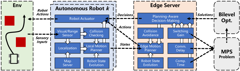
Figure 2: Architecture of EARN, which consists of a planning-aware decision-making module for planner switching and hierarchical motion planners deployed at robots and edge server.

III Tightly Coupled Decision-Making and
Motion Planning

This section presents EARN, a T-DMMP framework based on HMP and MPS. The architecture of EARN is shown in Fig. 2, which adopts a planning-ware decision-making module $f_{D}$ to execute planner switching between a low-complexity local motion planner $f_{L}(\cdot)$ deployed at $K$ robots and a high-performance edge motion planner $f_{E}(\cdot)$ deployed at the edge server. The decision-making operates at a low frequency (e.g., $1$ Hz) and the motion planing operates at a high frequency (e.g., $10\sim 100$ Hz). In the following subsections, we first present the HMP and MPS models in details, and then discuss the benefits brought by EARN through a case study.

III-A Hierarchical Motion Planning

At the $t$-th time slot, the $k$-th robot (with $1\leq k\leq K$) estimates its current state ${}^{R}\mathbf{s}_{k,t}=(^{R}x_{k,t},^{R}y_{k,t},^{R}\theta_{k,t})$ and obstacle states $\{^{O}\mathbf{s}_{1,t},...,^{O}\mathbf{s}_{M,t}\}$ with ${}^{O}\mathbf{s}_{m,t}=(^{O}x_{m,t},^{O}y_{m,t},^{O}\theta_{m,t})$ (with $1\leq m\leq M$) using onboard visual and range sensors, where $(x_{i,t},y_{i,t})$ and $\theta_{i,t}$ are positions and orientations, of the $i$-th robot (if the upper-left subscript is $R$) and the $i$-th obstacle (if the upper-left subscript is $O$), respectively. The edge server collects the state information from $K$ robots and executes the decision-making module $f_{D}$ to determine the motion planners at all robots. The output of $f_{D}$ is a set of one-zero decision variables $\{\alpha_{1},\cdots,\alpha_{K}\}\in\{0,1\}^{K}$, where $\alpha_{k}=1$ represents the $k$-th robot being selected for edge planning and $\alpha_{k}=0$ represents the $k$-th robot being selected for local planning. Given $\alpha_{k}$, the local planner or edge planner can generate control vectors by minimizing the distances between the robot’s footprints $\{^{R}\mathbf{s}_{k,t}\}$ and the target waypoints $\{\mathbf{s}_{k,t}^{\diamond}\}$ over the prediction time horizon $[t,t+H]$. Specifically, the state evolution model ${}^{R}\mathbf{s}_{k,t+1}=E(^{R}\mathbf{s}_{k,t},^{R}\mathbf{u}_{k,t})$ is adopted to predict the trajectories $\{^{R}\mathbf{s}_{k,t+1},\cdots,^{R}\mathbf{s}_{k,t+H}\}$, where $H$ is the length of prediction horizon. For car-like robots, $E$ is determined by Ackermann kinetics:

$$E_{k}\left({}^{R}\mathbf{s}_{k,t},^{R}\mathbf{u}_{k,t}\right)=\mathbf{A}_{k,t}{\mathbf{s}_{k,t}}+\mathbf{B}_{k,t}{\mathbf{u}_{k,t}}+\mathbf{c}_{k,t},~{}\forall k,t,$$ (1)

where $(\mathbf{A}_{k,t}$, $\mathbf{B}_{k,t}$, $\mathbf{c}_{k,t})$ are coefficient matrices defined in equations (8)–(10) of [8, Sec. III-B]. With the above state evolution model, we can estimate state ${}^{R}\mathbf{s}_{k,t+h+1}=E_{k}(^{R}\mathbf{s}_{k,t+h},^{R}\mathbf{u}_{k,t+h})$ for any $h\in[0,H-1]$ and the full-shape distance ${\bf{dist}}\left({}^{R}\mathbf{s}_{k,t+h},^{O}\mathbf{s}_{m,t+h}\right)$ between the $k$-th robot and the $m$-th obstacle at the $t$-th time slot (the function $\bf{dist}$ is detailed in Section IV-B). Consequently, the HMP problem for the $k$-th robot is formulated as

$$\min\limits_{\{^{R}\mathbf{s}_{k,t+h},^{R}\mathbf{u}_{k,t+h}\}_{h=0}^{H}}~{}~{}\sum^{H}_{h=0}\left\|{}^{R}\mathbf{s}_{k,t+h}-\mathbf{s}_{k,t+h}^{\diamond}\right\|^{2}$$ (2a)

$$\text{ s.t. }~{}~{}^{R}\mathbf{s}_{k,t+h+1}=E_{k}(^{R}\mathbf{s}_{k,t+h},^{R}\mathbf{u}_{k,t+h}),~{}\forall h,$$ (2b)

$$~{}~{}~{}~{}~{}~{}~{}~{}\mathbf{u}_{\min}\preceq^{R}\mathbf{u}_{k,t+h}\preceq\mathbf{u}_{\max},~{}\forall h,$$ (2c)

$$~{}~{}~{}~{}~{}~{}~{}~{}\mathbf{a}_{\min}\preceq{{}^{R}\mathbf{u}_{k,t+h+1}}-{{}^{R}\mathbf{u}_{k,t+h}}\preceq\mathbf{a}_{\max},~{}\forall h,$$ (2d)

$$~{}~{}~{}~{}~{}~{}~{}~{}\Psi\left({}^{R}\mathbf{s}_{k,t+h},{{}^{O}\mathbf{s}}_{m,t+h}|\alpha_{k}\right)\geq 0,~{}\forall m\in\mathcal{M}(k),h,$$ (2e)

where $\Psi$ is a conditional collision avoidance function

$$\Psi\left({}^{R}\mathbf{s}_{k,t+h},^{O}\mathbf{s}_{m,t+h}|\alpha_{k}\right)$$

$$=\alpha_{k}\left({\bf{dist}}\left({}^{R}\mathbf{s}_{k,t+h},^{O}\mathbf{s}_{m,t+h}\right)-d_{\text{safe}}\right),$$ (3)

and $\mathcal{M}(k)$ is the set of obstacles within the local map of robot $k$, and its cardinality is denoted as $|\mathcal{M}(k)|$. Constants ${\mathbf{u}_{\min}}$ (${\mathbf{a}_{\min}}$) and ${\mathbf{u}_{\max}}$ (${\mathbf{a}_{\max}}$) are the minimum and maximum values of the control (acceleration) vector, respectively. It can be seen that the full-shape collision avoidance constraints exist when $\alpha_{k}=1$, and the optimal control vector ${}^{R}\mathbf{u}_{k,t}^{*}$ to problem (2) leads to a proactive collision avoidance policy. In this case, problem (2) is solved at the edge server and we define $f_{E}(^{R}\mathbf{s}_{k,t},\{^{O}\mathbf{s}_{m,t}\}_{m=1}^{M})={{}^{R}\mathbf{u}}_{k,t}^{[1]}={{}^{R}\mathbf{u}}_{k,t}^{*}$. In contrast, when $\alpha_{k}=0$, the collision avoidance constraints are discarded, and the optimal ${{}^{R}\mathbf{u}}_{k,t}^{*}$ to problem (2) leads to a reactive collision avoidance policy, which is replaced by braking action $\mathbf{u}_{B}$ whenever the robot sensor detects obstacles ahead within a certain braking distance $d_{\mathrm{B}}$. In this case, problem (2) is solved at the robot $k$ and we define $f_{L}(^{R}\mathbf{s}_{k,t},\{^{O}\mathbf{s}_{m,t}\}_{m=1}^{M})={{}^{R}\mathbf{u}}_{k,t}^{[0]}$, where ${{}^{R}\mathbf{u}}_{k,t}^{[0]}$ takes the value of ${}^{R}\mathbf{u}_{k,t}^{*}$ or $\mathbf{u}_{B}$. Combining the two cases, the action of the $k$-th robot is given by

$$\mathbf{u}_{k,t}=\left\{\begin{array}[]{ll}f_{E}(^{R}\mathbf{s}_{k,t},\{^{O}\mathbf{s}_{m,t}\}_{m=1}^{M}),&\mathrm{if}~{}\alpha_{k}=1\\ f_{L}(^{R}\mathbf{s}_{k,t},\{^{O}\mathbf{s}_{m,t}\}_{m=1}^{M}),&\mathrm{if}~{}\alpha_{k}=0\end{array}\right..$$ (4)

III-B Model Predictive Switching

The proposed framework aims to find the optimal decision variables $\{\alpha_{k}^{*}\}$ by maximizing the expected switching gain over all robots under the communication and computation resource constraints.

• The communication latency $D_{k}$ between the $k$-th robot and the edge server should be smaller than a certain threshold $D_{\mathrm{th}}$ if $\alpha_{k}=1$, i.e., $\alpha_{k}D_{k}(^{R}\mathbf{s}_{k,t})\leq D_{\mathrm{th}}$.

• The total computation time at the server should not exceed a certain threshold $C_{\mathrm{th}}$, i.e., $\sum_{k}\alpha_{k}C_{k}(H,|\mathcal{M}(k)|)\leq C_{\mathrm{th}}$, where $C_{k}$ is determined by the prediction time length $H$ and the number of obstacles $\mathcal{M}(k)$.

• The expected switching gain is defined as the difference between the moving distance of planner $f_{L}$ and that of $f_{E}$ at time $t+H$, which is

  $$G_{k}\left({{}^{R}\mathbf{s}_{k,t}},\{^{O}\mathbf{s}_{m,t}\},f_{E},f_{L}\right)$$

  $$=\|^{R}\mathbf{s}_{k,t+H}^{[1]}-{{}^{R}\mathbf{s}_{k,t}}\|^{2}-\|^{R}\mathbf{s}_{k,t+H}^{[0]}-{{}^{R}\mathbf{s}_{k,t}}\|^{2}.$$ (5)

  where ${}^{R}\mathbf{s}_{k,t+H}^{[1]}$ is the optimal solution of ${}^{R}\mathbf{s}_{k,t+H}$ to problem (2) if $\alpha_{k}=1$ and ${}^{R}\mathbf{s}_{k,t+H}^{[0]}$ is the optimal solution of ${}^{R}\mathbf{s}_{k,t+H}$ to problem (2) if $\alpha_{k}=0$.

Based on the above analysis, the T-DMMP is formulated as the following MPS problem

$$\max\limits_{\{\alpha_{k}\}_{k=1}^{K}}~{}~{} \sum_{k=1}^{K}\alpha_{k}G_{k}\left({{}^{R}\mathbf{s}_{k,t}},\{^{O}\mathbf{s}_{m,t}\},f_{E},f_{L}\right)$$ (6a)

s.t. $$\{^{R}\mathbf{s}_{k,t+H}^{[\alpha_{k}]}\}=\mathop{\arg\,\min\limits_{\{^{R}\mathbf{s}_{k,t+h},^{R}\mathbf{u}_{k,t+h}\}_{h=0}^{H}}}\Big{\{}\sum^{H}_{h=0}$$

$$\left\|{}^{R}\mathbf{s}_{k,t+h}-\mathbf{s}_{k,t+h}^{\diamond}\right\|^{2}:(\ref{problemAb})-(\ref{problemAe})\Big{\}},~{}\forall k,$$ (6b)

$$\alpha_{k}D_{k}(^{R}\mathbf{s}_{k,t})\leq D_{\mathrm{th}},~{}\forall k,$$ (6c)

$$\sum_{k=1}^{K}\alpha_{k}C_{k}(H,|\mathcal{M}(k)|)\leq C_{\mathrm{th}},$$ (6d)

$$\alpha_{k}\in\{0,1\},~{}\forall k.$$ (6e)

It can be seen that the MPS formulation requires joint considerations of planning, communications, computations, and scenarios as illustrated in Fig. 3. Inappropriate decisions would lead to collisions due to either local/edge computation timeout or communication timeout.

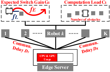
Figure 3: Tightly-coupled design of EARN

III-C Case Study

To demonstrate the practicability and feasibility of the proposed framework, a case study is conducted for the 5-robot system shown in Fig. 1. In particular, we consider two embedded computing chips, i.e., NVIDIA Jetson Nano and NVIDIA Orin NX, and two motion planners, i.e., point-mass PF [4] and full-shape RDA [8]. The power and price of Jetson Nano are 10 Watts and 150 $ each. The power and price of Orin NX are 25 Watts and 1000 $ each. Based on our experimental data, a frequency of $50\,$Hz can be achieved for PF on both chips. As for RDA, it can only be executed at a frequency of $2\,$Hz on Jetson Nano, and $30\,$Hz to $50\,$Hz on Orin NX, when the number of obstacles is $10$ [8].

Now we consider three schemes: 1) Onboard navigation I, with all robots equipped with Jetson Nano; 2) Onboard navigation II, with all robots equipped with Orin NX; 3) EARN, with 4 low-cost robots equipped with Jetson Nano and 1 robotic edge server equipped with Orin NX. The latency, power, and price of different schemes are illustrated in Fig. 4 (the values of all performance metrics are normalized to their associated maximum values). It can be seen from Fig. 4 that: 1) The average computation latency of EARN ($20$ ms) is significantly smaller than that of the onboard navigation-I ($500$ ms); 2) EARN ($65$ W) is more energy efficient than the on-board navigation II ($125$ W); 3) The total system cost of EARN is significantly smaller than that of onboard navigation-II (1600 $ versus 5000 $). In summary, EARN achieves much faster robot navigation compared to on-board navigation I, and more energy and cost efficient navigation compared to onboard navigation II. Moreover, EARN is not sensitive to communication uncertainties, as each robot can always switch to a local PF planner whenever communication outage occurs. This is in contrast to conventional fully edge offloading schemes [19].

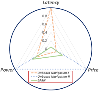
Figure 4: Benefits brought by EARN

IV Algorithm Design for Decision-Making and Motion Planning

IV-A Decision-Making

To solve the MPS problem, we need mathematical expressions of the communication latency $D_{k}$, the computation latency $C_{k}$, and the planner switching gain $G_{k}$ as shown in Fig. 3.

First, the function $D_{k}$ is determined by pinging the communication latency between a mobile robot and an edge server under different distances in an indoor WIFI network at our laboratory. According to the measurements, the communication latency $D_{k}$ is approximated as $D_{k}\in\mathcal{U}(80,120)$ in ms if the distance from ${}^{R}\mathbf{s}_{k,t}$ to the server is larger than $10\,$m and $D_{k}\in\mathcal{U}(10,50)$ in ms otherwise, where $\mathcal{U}(a,b)$ represents uniform distribution within interval $[a,b]$. On the other hand, for outdoor scenarios, due to larger transmit power of the robot and reduced blockage effects, the communication coverage would increase, and we set $D\in\mathcal{U}(50,150)$ in ms if the distance from ${}^{R}\mathbf{s}_{k,t}$ to the server is larger than $30\,$m and $D\in\mathcal{U}(10,50)$ in ms otherwise [22].

Next, we determine the computing latency $C_{k}$. Since a common motion planner has a polynomial-time computational complexity, without loss of generality, we can write $C_{k}$ as

$$C_{k}=\gamma H|\mathcal{M}(k)|^{p}+\tau,$$ (7)

where $\gamma$ and $\tau$ are hardware-dependent hyper-parameters estimated from historical experimental data. Moreover, $p$ is the order of complexity, which ranges from $1$ to $3.5$ and depends on the motion planner.

Finally, we determine $G_{k}$, which is coupled with the motion planning algorithms $f_{E}$ and $f_{L}$. In particular, if $\|{{}^{R}\mathbf{s}}_{k,t}-{{}^{O}\mathbf{s}}_{m,t}\|>d_{\mathrm{B}}$, we have $G_{k}=0$, since the local planning problem is a relaxation of the edge planning problem. On the other hand, if $\|^{R}\mathbf{s}_{k,t}-^{O}\mathbf{s}_{m,t}\|\leq d_{\mathrm{B}}$, then $\|^{R}\mathbf{s}_{k,t+H}^{[0]}-{{}^{R}\mathbf{s}_{k,t}}\|^{2}=0$ as the braking signal is generated and the robot stops. Combining the above two cases, $G_{k}$ is equivalently written as

$$G_{k}=I_{k}\,\|^{R}\mathbf{s}_{k,t+H}^{[1]}-{{}^{R}\mathbf{s}_{k,t}}\|^{2},$$ (8)

where

$$I_{k}=\left\{\begin{array}[]{ll}1,&\mathrm{if}~{}\|^{R}\mathbf{s}_{k,t}-{{}^{O}\mathbf{s}_{m,t}}\|\leq d_{\mathrm{B}},{{}^{O}\mathbf{s}_{m,t}}\in\mathcal{W}_{k}\\ 0,&\mathrm{otherwise}\end{array}\right.,$$ (9)

and $\mathcal{W}_{k}$ contains the obstacles that are on the same lane with the robot $k$.

Based on the above derivations of $D_{k}$, $C_{k}$, and $G_{k}$, the original MPS problem (6) is transformed into

$$\max\limits_{\{\alpha_{k}\}_{k=1}^{K}}~{}~{} \sum_{k=1}^{K}\alpha_{k}I_{k}\|^{R}\mathbf{s}_{k,t+H}^{[1]}-{{}^{R}\mathbf{s}_{k,t}}\|^{2}$$ (10a)

s.t. $$(\ref{problemBb}),(\ref{problemBc}),(\ref{problemBe}),$$ (10b)

$$\sum_{k=1}^{K}\alpha_{k}\gamma H|\mathcal{M}(k)|^{p}+\tau\leq C_{th}.$$ (10c)

This is a B-MINLP problem due to the constraints (6b) and (6e). A naive approach is to solve the inner problem (6b) for all robots and conduct an exhaustive search over $\{\alpha_{k}\}$. However, the resultant complexity would be $\mathcal{O}(2^{K})$, which cannot meet the frequency requirement of the decision-making module. To this end, we propose a low-complexity method summarized in Algorithm 1, which consists of three sequential steps: 1) Prune out impossible solutions for space reduction (lines 3 to 9:); 2) Leverage parallel motion planning for fast trajectory computations (lines 10 to 12); 3) Put $\{\alpha_{k}=0\}_{k\in\mathcal{I}}$ and $\{^{R}\mathbf{s}_{k,t}^{[1]}\}_{k\in\mathcal{A}}$ into problem (10), and solve the resultant problem using integer linear programming, e.g., CVXPY (line 13).

1 Initialize the robots’ states $\{^{R}\mathbf{s}_{k,t+h}\}$, robots’ actions $\{^{R}\mathbf{u}_{k,t+h}\}$, $D_{th}$, and $\mathcal{A}=\mathcal{I}=\emptyset$

2 Estimate $D_{k}$ and $C_{k}$ using historical data

3 for robot $k=1,\cdots,K$ do

4       if $\alpha_{k}=1$ satisfies (10c) and $I_{k}=1$ then

5            Set $\alpha_{k}=1$ and update $\mathcal{A}\leftarrow\{k\}\cup\mathcal{A}$

6      else

7            Set $\alpha_{k}=0$ and update $\mathcal{I}\leftarrow\{k\}\cup\mathcal{I}$

8       end if

9      

10 end for

11for robot $k\in\mathcal{A}$ do

12       Compute $\{{{}^{R}\mathbf{s}_{k,t}^{[1]}}\}$ in (6b) using PDD

13 end for

Solve (10) with integer linear programming.

Algorithm 1 Planning-Aware Decision-Making

IV-B Motion Planning

When $\alpha_{k}=0$, the local motion planner is adopted and the resultant planning problem is

$$\min\limits_{\{^{R}\mathbf{s}_{k,t+h},^{R}\mathbf{u}_{k,t+h}\}_{h=0}^{H}}~{}~{} \sum^{H}_{h=0}\left\|{}^{R}\mathbf{s}_{k,t+h}-\mathbf{s}_{k,t+h}^{\diamond}\right\|^{2}$$ (11a)

s.t. $$(\ref{problemAb}),(\ref{problemAc}),(\ref{problemAd})$$ (11b)

The above problem can be independently solved at each robot since there is no coupling among different $k$. Denoting the solution as $\{^{R}\mathbf{s}_{k,t}^{*},^{R}\mathbf{u}_{k,t}^{*}\}$, we set the action of robot $k$ as

$$^{R}\mathbf{u}_{k,t}^{[0]}=\left\{\begin{array}[]{ll}\mathbf{u}_{\mathrm{B}},&\mathrm{if}~{}\|^{R}\mathbf{s}_{k,t}-{{}^{O}\mathbf{s}_{m,t}}\|\leq d_{\mathrm{B}},{{}^{O}\mathbf{s}_{m,t}}\in\mathcal{W}_{k}\\ {}^{R}\mathbf{u}_{k,t}^{*},&\mathrm{otherwise}\end{array}\right.,$$ (12)

where $d_{\mathrm{B}}$ is the minimum distance for planner $f_{L}$ to take braking actions. The set $\mathcal{W}_{k}$ represents the target lane, which contain points close to the target waypoints $\{\mathbf{s}_{k,t}^{\diamond}\}$, and is given by

$$\mathcal{W}_{k}=\left\{\mathbf{s}:\|\mathbf{s}-\mathbf{s}_{k,t}^{\diamond}\|\leq\delta,~{}\forall t\right\},$$ (13)

where $\delta$ is the width of the lane.

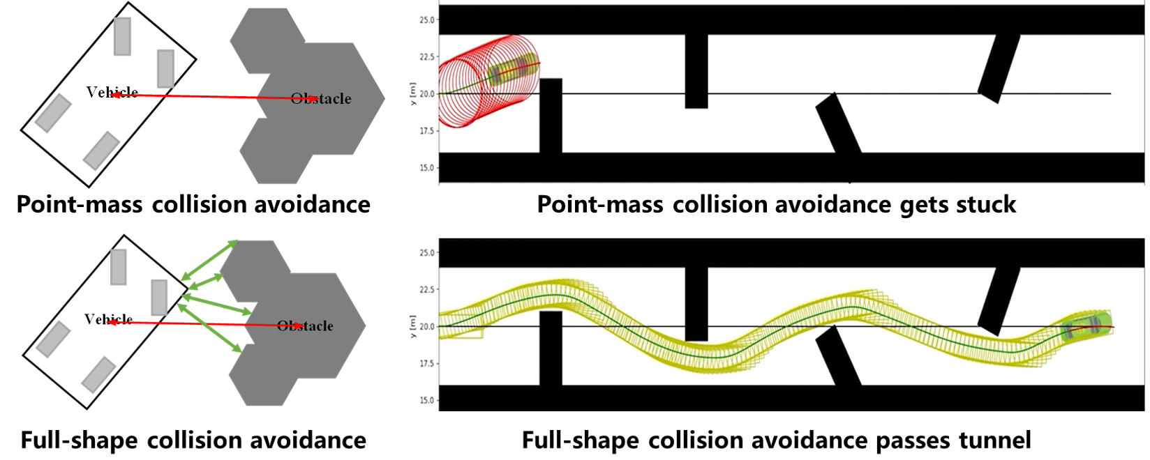
Figure 5: Comparison between point-mass obstacle model and non-point-mass obstacle model. The red line represents the distance computed by the conventional approach, while the proposed PDD computes the actual distance between the two objects (i.e., the minimum value of the green lines).

When $\alpha_{k}=1$, the edge motion planner is adopted and the resultant planning problem is

$$\min\limits_{\{^{R}\mathbf{s}_{k,t+h},^{R}\mathbf{u}_{k,t+h}\}_{h=0}^{H}}~{}~{} \sum^{H}_{h=0}\left\|{}^{R}\mathbf{s}_{k,t+h}-\mathbf{s}_{k,t+h}^{\diamond}\right\|^{2}$$ (14a)

s.t. $$(\ref{problemAb}),(\ref{problemAc}),(\ref{problemAd}),(\ref{problemAe})$$ (14b)

It can be seen that different from the case of $\alpha_{k}=0$, the effect of obstacles is now considered. Here, in contrast to conventional approaches that model the obstacle as a point or a ball [23], the obstacles’ shapes are taken into account and modeled as polyhedrons as in [3, 8]. As shown in Fig. 5, the red line represents the distance computed by conventional approaches, while we compute the actual distance between the two objects (i.e., the minimum value of the green lines). It can be seen that the red line is much longer than the green lines, and navigation based on the red line may get stuck in dense environments. However, if the obstacle shapes are considered, the computation speed would become a challenge, which hinders the practical application of [3, 8]. This motivates us to develop a PDD motion planner for fast parallel optimization. Note that PDD is different from our previous work, RDA [8], as PDD incorporates the online calibration of penalty parameters into RDA, leading to convergence guaranteed robot navigation.

To begin with, we review the collision model between the $k$-th robot and the $m$-th obstacle in our previous work [8]. Specifically, a set ${}^{R}\mathbb{G}_{k,t}$ is adopted to represent the geometric region occupied by the robot, which is related to its state ${}^{R}\mathbf{s}_{k,t}$ and its shape ${}^{R}\mathbb{Z}_{k}$:

$${}^{R}\mathbb{G}_{k,t}(^{R}\mathbf{s}_{k,t},^{R}\mathbb{Z}_{k}) =\mathbf{R}_{k,t}(^{R}\mathbf{s}_{k,t})\mathbf{z}+\mathbf{p}_{k,t}(^{R}\mathbf{s}_{k,t}).$$ (15)

where $\mathbf{R}_{k,t}\in{\mathbb{R}^{{3}\times{3}}}$ is a rotation matrix related to ${}^{R}\theta_{k,t}$, $\mathbf{p}_{k,t}\in{\mathbb{R}^{{3}}}$ is a translation vector related to $(^{R}x_{k,t},{{}^{R}y_{k,t}})$, and ${{}^{R}\mathbb{Z}_{k}}=\{\mathbf{z}\in{\mathbb{R}^{3}}|^{R}\mathbf{G}_{k}\mathbf{z}\leq{{}^{R}\mathbf{g}_{k}}\}$, where $\mathbf{G}_{k}\in{\mathbb{R}^{l_{k}\times 3}}$ and $\mathbf{g}_{k}\in{\mathbb{R}^{l_{k}}}$, with $l_{k}$ being the number of edges for the $k$-th robot. Similarly, the $m$-th obstacle can be represented by ${}^{O}\mathbb{G}_{m,t}=\{\mathbf{z}\in{\mathbb{R}^{3}}|{{}^{O}\mathbf{G}_{m,t}}\mathbf{z}\leq{{}^{O}\mathbf{g}_{m,t}}\}$.

To determine whether the $k$-th robot collides with the $m$-th obstacle, the distances between any two points within ${}^{R}\mathbb{G}_{m,t}$ and ${}^{O}\mathbb{G}_{m,t}$ are computed. Then we check if any distance is smaller than $d_{\mathrm{safe}}$. If so, a collision is likely to happen; otherwise, no collision occurs. Consequently, constraint (2e) is equivalently written as

$${\bf{dist}}({{}^{R}\mathbb{G}_{k,t+h}},{{}^{O}\mathbb{G}_{m,t+h}})\geq{d_{\mathrm{safe}}},~{}\forall m\in\mathcal{M}(k),h,$$ (16)

Function $\bf{dist}$ is not analytical, but can be equivalently transformed into its dual from represented by variables $\bm{\lambda}_{k,m,h}\in{\mathbb{R}^{l_{m}}}$, $\bm{\mu}_{k,m,h}\in{\mathbb{R}^{l_{k}}}$, and $z_{k,m,h}\in\mathbb{R}$ [3, 8], which represent our attentions on different edges of robots and obstacles. After this transformation, instead of directly solving the dual problem using optimization softwares [3] or ADMM [8], we construct the augmented Lagrangian of (14) as

$$\mathop{\mathrm{min}}_{\begin{subarray}{c}\{^{R}\mathbf{s}_{k,t+h},^{R}\mathbf{u}_{k,t+h}\}\in\mathcal{X}_{k},\\ \{(\bm{\lambda}_{k,m,h},\bm{\mu}_{k,m,h},z_{k,m,h})\in\mathcal{Y}_{k,m,t}\}\end{subarray}}\mathcal{L}_{k}\Big{(}\{^{R}\mathbf{s}_{k,t+h},{{}^{R}\mathbf{u}_{k,t+h}}\},$$

$$~{}~{}~{}~{}~{}~{}~{}\{\bm{\lambda}_{k,m,h},\bm{\mu}_{k,m,h},z_{k,m,h}\};\rho,\{\bm{\zeta}_{k,m,h},\xi_{k,m,h}\}\Big{)},$$ (17)

where $\mathcal{X}_{k}$ is the set for constraints (2b)–(2d), $\mathcal{Y}_{k}$ is the set for constraint

$$\begin{array}[]{l}\bm{\lambda}_{k,m,h}\succeq\mathbf{0},\\ {\left\|{{{}^{O}\mathbf{G}_{m,t+h}^{T}}\bm{\lambda}_{k,m,h}}\right\|}\leq 1,\\ \bm{\mu}_{k,m,h}{\succeq}\mathbf{0},\\ z_{k,m,h}\geq 0,\end{array}$$ (18)

$\{\bm{\zeta}_{k,m,h},\xi_{k,m,h}\}$ are slack variables, $\rho$ is the penalty parameter, and

$$\mathcal{L}_{k}=\sum^{H}_{h=0}\left\|{}^{R}\mathbf{s}_{k,t+h}-\mathbf{s}_{k,t+h}^{\diamond}\right\|^{2}+\frac{\rho}{2}\sum_{h=0}^{H}\sum_{m=0}^{M}\Big{\|}{\bm{\mu}_{k,m,h}^{T}}{{}^{R}\mathbf{G}_{k}}$$

$$+{\bm{\lambda}_{k,m,h}^{T}}{{}^{O}\mathbf{G}_{m,t+h}}\mathbf{R}_{k,t+h}+\bm{\zeta}_{k,m,h}\Big{\|}^{2}$$

$$+\frac{\rho}{2}\sum_{h=0}^{H}\sum_{m=0}^{M}\Big{(}\bm{\lambda}_{k,m,h}^{T}{{}^{O}\mathbf{G}_{m,t+h}}\mathbf{p}_{k,t+h}-{\bm{\lambda}_{k,m,h}^{T}}{{}^{O}\mathbf{g}_{m,t+h}}$$

$$-{\bm{\mu}_{k,m,h}^{T}}{{}^{R}\mathbf{g}_{k}}-z_{k,m,h}-{d}_{\mathrm{safe}}+\xi_{k,m,h}\Big{)}^{2}.$$ (19)

1 Initialize the robot state $\{^{R}\mathbf{s}_{k,t+h}\}$, the robot action $\{^{R}\mathbf{u}_{k,t+h}\}$, attentions $\{\bm{\lambda}_{k,m,h},\bm{\mu}_{k,m,h},z_{k,m,h}\}$, and parameters $\{\beta,\rho,\eta_{iter}\}$

2 for iteration $iter=1,2,\cdots$ do

3       $\{^{R}\mathbf{s}_{k,t+h},^{R}\mathbf{u}_{k,t+h}\}\leftarrow\mathop{\mathrm{argmin}}_{\{^{R}\mathbf{s}_{k,t+h},^{R}\mathbf{u}_{k,t+h}\}\in\mathcal{X}_{k}}\mathcal{L}_{k}$

4       $(\bm{\lambda}_{k,m,h},\bm{\mu}_{k,m,h},z_{k,m,h})\leftarrow\mathop{\mathrm{argmin}}_{(\bm{\lambda}_{k,m,h},\bm{\mu}_{k,m,h},z_{k,m,h})\in\mathcal{Y}_{k,m,h}}\mathcal{L}_{k},~{}\forall m,h$

5       if $\Phi\left(\{\bm{\lambda}_{k,m,h},\bm{\mu}_{k,m,h},z_{k,m,h}\}\right)\leq\eta_{iter}$ then

6            Update $\{\bm{\zeta}_{k,m,h},\xi_{k,m,h}\}$ using (21),$~{}\forall m,h$

7      else

8            Update $\rho\leftarrow\beta\rho$

9       end if

10      

11 end for

Algorithm 2 PDD motion planner

To solve problem (17), the PDD motion planner is proposed, which is summarized in Algorithm 2. In particular, we first optimize the robot states and actions with all other variables fixed via CVXPY as shown in line $3$ of Algorithm 2. Next, we optimize the collision attentions with all other variables fixed via CVXPY as shown in line $4$ of Algorithm 2. Lastly, from lines $5$ to $9$, we either execute dual update or penalty update based on the residual function $\Phi$:

$$\Phi\left(\{\bm{\lambda}_{k,m,h},\bm{\mu}_{k,m,h},z_{k,m,h}\}\right)=$$

$$\max\Big{\{}\max\limits_{h,m}~{}\Big{\|}{\bm{\mu}_{k,m,h}^{T}}{{}^{R}\mathbf{G}_{k}}+{\bm{\lambda}_{k,m,h}^{T}}{{}^{O}\mathbf{G}_{m,t+h}}\mathbf{R}_{k,t+h}\Big{\|}_{\infty},$$

$$\quad\quad~{}~{}\max\limits_{h,m}~{}\Big{|}\bm{\lambda}_{k,m,h}^{T}{{}^{O}\mathbf{G}_{m,t+h}}\mathbf{p}_{k,t+h}-{\bm{\lambda}_{k,m,h}^{T}}{{}^{O}\mathbf{g}_{m,t+h}}$$

$$\quad\quad~{}~{}-{\bm{\mu}_{k,m,h}^{T}}{{}^{R}\mathbf{g}_{k}}-z_{k,m,h}-{d}_{\mathrm{safe}}\Big{|}\Big{\}}.$$ (20)

For dual update (line 6), we compute $\bm{\zeta}_{k,m,h}\},\{\xi_{k,m,h}$ using subgradient method as follows

$$\bm{\zeta}_{k,m,h}\leftarrow\bm{\zeta}_{k,m,h}+\Big{(}{\bm{\mu}_{k,m,h}^{T}}{{}^{R}\mathbf{G}_{k}}+{\bm{\lambda}_{k,m,h}^{T}}{{}^{O}\mathbf{G}_{m}}\mathbf{R}_{k,t+h}\Big{)},$$

$$\xi_{k,m,h}\leftarrow\xi_{k,m,h}+\Big{(}\bm{\lambda}_{k,m,h}^{T}{{}^{O}\mathbf{G}_{m,t+h}}\mathbf{p}_{k,t+h}-{\bm{\lambda}_{k,m,h}^{T}}{{}^{O}\mathbf{g}_{m,t+h}}$$

$$\quad\quad\quad\quad-{\bm{\mu}_{k,m,h}^{T}}{{}^{R}\mathbf{g}_{k}}-z_{k,m,h}-{d}_{\mathrm{safe}}\Big{)}.$$ (21)

For penalty update (line 8), we update

$$\rho\leftarrow\beta\rho,$$ (22)

with $\beta\geq 1$ being an increasing factor. According to [18, Theorem 3.1], Algorithm 2 is guaranteed to converge to a KKT solution to problem (17). The complexity of PDD is given by

$$\mathrm{Comp}_{k} =\mathcal{O}((5H)^{3.5}+H\sum_{m\in\mathcal{M}(k)}(l_{m}+l_{k})^{3.5}$$

$$\quad{}{}+H|\mathcal{M}(k)|(l_{m}+l_{k})).$$ (23)

V Experiments

V-A Implementation

We implemented the proposed EARN system using Python in Robot Operating System (ROS). The high-fidelity CARLA simulation platform [24] is used for evaluations, which adopts unreal engine for high-performance rendering and physical engine for fine-grained dynamics modeling as shown in Fig. 1. Our EARN system is connected to CARLA via ROS bridge [25] and data sharing is realized via ROS communications, where the nodes publish or subscribe ROS topics that carry the sensory, state, or action information. We simulate two outdoor scenarios and one indoor scenario. All simulations are implemented on a Ubuntu workstation with a $3.7$ GHZ AMD Ryzen 9 5900X CPU and an NVIDIA $3090$ Ti GPU.

We also implement EARN in a real-world multi-robot platform, where each robot has four wheels and can adopt Ackermann or differential steering. The robot named LIMO has a 2D lidar, RGBD camera, and an onboard NVIDIA Jetson Nano computing platform for executing the SLAM and local motion planning packages. The edge server is a manually controlled wheel-legged robot, Direct Drive Tech (DDT) Diablo, which has a 3D livox lidar and an onboard NVIDIA Orin NX computing platform for executing the SLAM and edge motion planning packages. The Diablo is also equipped with a mobile phone to provide a local wireless access point.

To obtain the value of parameters involved in model (7), we execute the PDD motion planning in Algorithm 2 on the AMD Ryzen 9 and NVIDIA Orin NX chips. The experimental data of computation time (ms) versus the number of prediction horizons $H$ and the number of obstacles $|\mathcal{M}(k)|$ is shown in Fig. 6. It can be seen that the computation time of PDD scales linearly with $H$ and $|\mathcal{M}_{k}|$, which corroborates the complexity analysis in equation (23). As such, the value of parameter $p$ is set to 1. The computation time ranges from less than $10\,$ms to $200\,$ms, corresponding to a planning frequency of $0.5\,$Hz to over $100\,$Hz. The parameters $\gamma,\tau$ are obtained by fitting the function $C_{k}=\gamma H|\mathcal{M}_{k}|+\tau$ to the experimental data in Fig. 6 using weighted least squares, and is given by $\gamma^{*}=0.6$ and $\tau^{*}=12\,$ms for ADM Ryzen 9 and $\gamma^{*}=1$ and $\tau^{*}=20\,$ms for NVIDIA Orin NX.

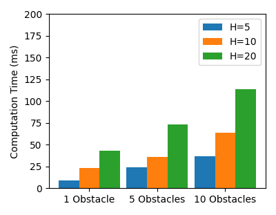
(a) AMD Ryzen 9

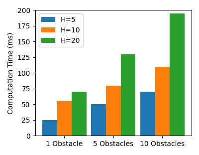
(b) NVIDIA Orin NX

Figure 6: Computation time (ms) of PDD planner versus the number of prediction horizons $H$ and obstacles $|\mathcal{M}(k)|$.

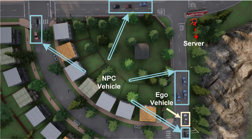
(a) Crossroad scenario

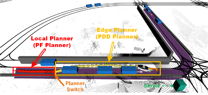
(b) Overtaking performed by EARN

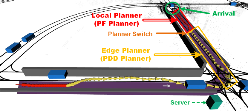
(c) EARN

(d) PF

(e) PDD-Edge

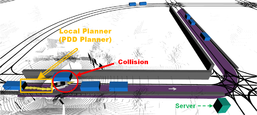
(f) PDD-Local

Figure 7: Crossroad scenario in CARLA Town04 and trajectories of different schemes. Trajectories generated by the local and edge motion planners are marked in red and yellow, respectively.

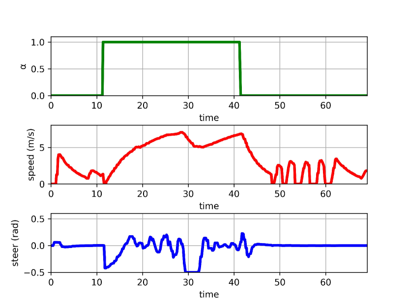
(a) EARN

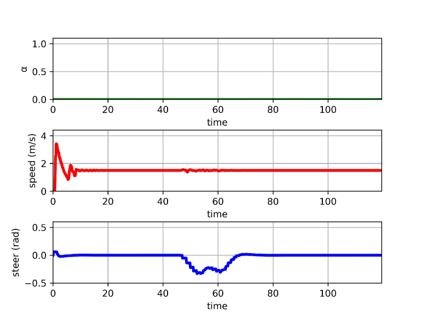
(b) PF

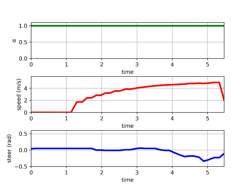
(c) PDD-Edge

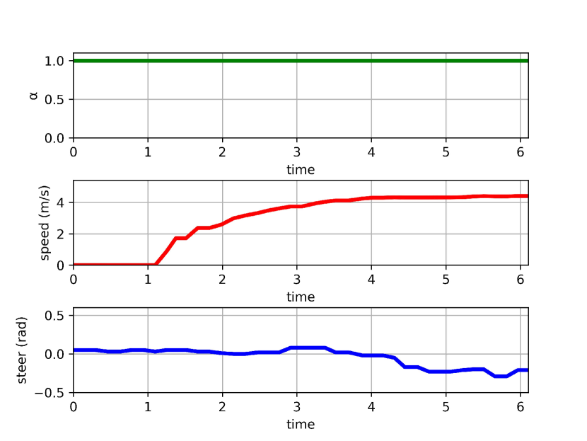
(d) PDD-Local

Figure 8: Comparison of vehicle states and actions in crossroad scenario.

V-B Benchmarks

We compare our method to the following baselines:

• Path Following (PF) planner [4];

• Collision avoidance MPC (CAMPC) [23], which models each obstacle as a single point and determines the collision condition by computing the distance between the position of this point and the ego-robot;

• RDA planner [8], which solves (14) in parallel via ADMM;

• PDD-Edge, or PDD-E for short, which executes PDD planning at the edge server by combining the proposed PDD planner and the idea of [26].

• PDD-Local, or PDD-L for short, which executes the proposed PDD planner at the local robot.

• EDF, which is a hierarchical motion planning scheme where robots are opportunistically selected for edge computing using a non-preemptive earliest deadline first (EDF) policy [16].

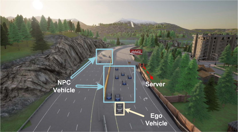
(a) Dense traffic scenario

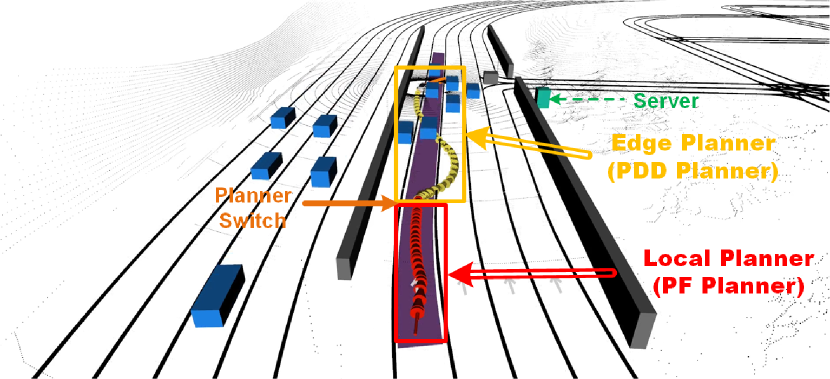
(b) PDD (snapshot 1)

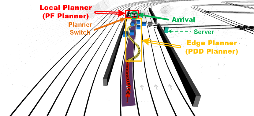
(c) PDD (snapshot 2)

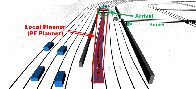
(d) PF

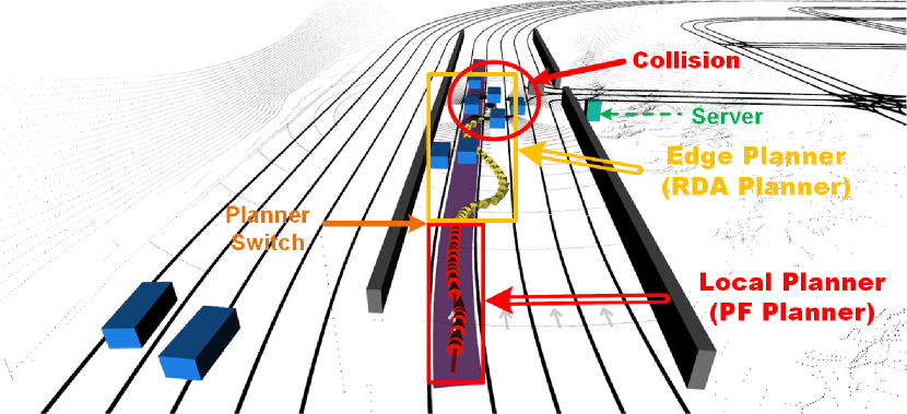
(e) RDA

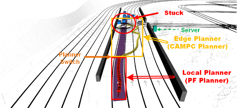
(f) CAMPC

Figure 9: Dense traffic scenario in CARLA Town04 and comparison of different trajectories. Trajectories generated by the local and edge motion planners are marked in red and yellow, respectively.

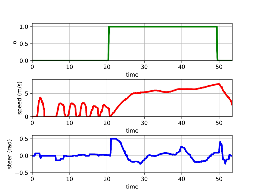
(a) PDD

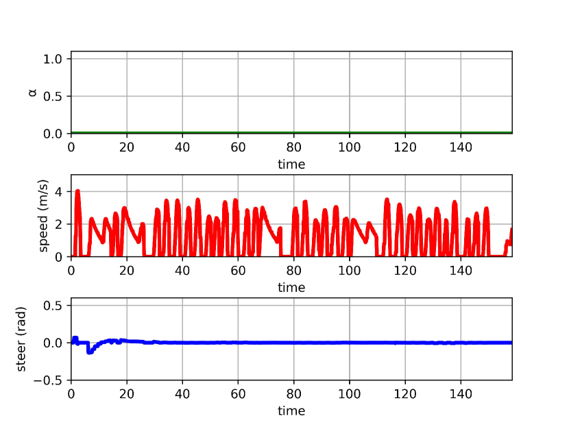
(b) PF

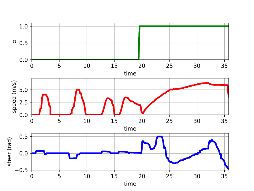
(c) RDA

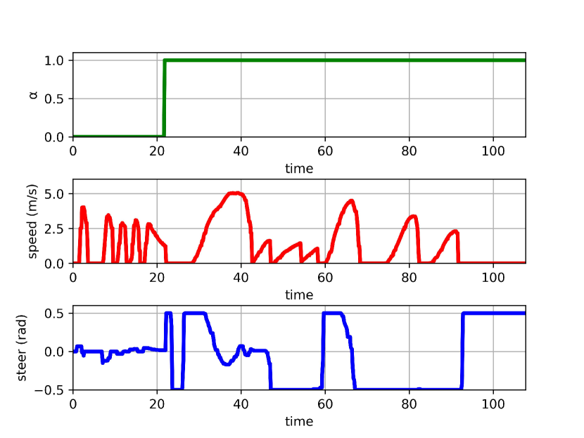
(d) CAMPC

Figure 10: Comparison of vehicle states and actions in dense traffic scenario.

V-C Single-Robot Simulation

We first evaluate EARN in single-robot outdoor scenarios. The server is assumed to be equipped with AMD Ryzen 9. The robot is assumed to be a low-cost logistic vehicle with its longitudinal wheelbase and lateral wheelbase being $2.87$ m and $1.75$ m, respectively. Based on these parameters, $(\mathbf{A}_{k,t}$, $\mathbf{B}_{k,t}$, $\mathbf{c}_{k,t})$ in (1) can be calculated. The braking distance for planner $f_{L}$ is set to $d_{\mathrm{B}}=8.0$ m and the safe distance for planner $f_{E}$ is set to $d_{\mathrm{safe}}=1$ m. The length of prediction horizon is set to $H=5$, with the time step between consecutive motion planning frames being $0.35$ s.

We consider a crossroad scenario in CARLA Town04 map, where the associated location of edge server, the starting/goal position of robot (with a random deviation of $3\,$m), and the positions of non-player character (NPC) vehicles are shown in Fig. 7a. In this scenario, the maximum number of NPC vehicles in the local map of robot is $5$. Using $H=5$ and $|\mathcal{M}|=5$, we have $C=27\,$ms when PDD is executed at the edge server. The computation time is more than $200$ ms when executed locally at the ego vehicle. The computation time of RDA is similar to that of PDD. The computation time of PF is negligible. The computation time of CAMPC is approximately $1/l_{m}$ of that of PDD, as CAMPC ignores the number of edges for each obstacle. The computation latency threshold is set to $C_{\mathrm{th}}=50\,$ms in Algorithm 1 according to the operational speed in the outdoor scenario.

The trajectories and control parameters generated by EARN, PF, PDD-E and PDD-L are illustrated in Fig. 7b–7f and Fig. 8. It is observed that both EARN and PF planner are able to navigate the robot to the destination without any collision. In contrast, PDD-E and PDD-L lead to collisions at $t=19.99\,$s and $t=20.78\,$s, respectively, due to nonsmooth actions caused by communication or computation latency.

The quantitative comparisons are presented in Table I, where the performance of each method is obtained by averaging $50$ trials. It can be seen that EARN reduces the average navigation time by 47% compared to PF, as EARN can switch the planner adaptively and utilize the computing resources at the server as shown in Fig. 7b and Fig. 7c. For instance, EARN executes the planner switching at $t=11.22\,$s as observed in Fig. 8a. This empowers the robot with the capability to overtake front low-speed obstacles and increase the maximum speed from $4.03\,$m/s to $7.06\,$m/s and the average speed from $1.67\,$m/s to $5.20\,$m/s, by leveraging edge motion planning through low-latency communication access. In contrast, the maximum speed and average speed achieved by the PF planner are merely $3.41\,$m/s and $1.50\,$m/s, respectively. Moreover, both PDD-E and PDD-L suffer from low success rate. This is because PDD-E and PDD-L involve either computation or communication latency, resulting in low end-to-end planning frequency. The proposed EARN achieves a success rate significantly higher than those of PDD-E and PDD-L (98% versus 64% and 58%), which demonstrates the necessity of planner switching introduced by EARN.

TABLE I: Comparison of navigation time and success rate

	EARN	PF	PDD-E	PDD-L
Avg Navigation Time (s)	64.23	120.54	49.24	64.75
Success Rate (%)	98%	100%	64%	58%

We also consider a dense traffic scenario in CARLA Town04 map as shown in Fig. 9a with tens of dynamic obstacles. This experiment is used to test the robustness of EARN in dynamic and complex environments. The trajectories and control vectors generated by PDD, PF, RDA, and CAMPC are illustrated in Fig. 9b–Fig. 9f and Fig. 10. In this challenging scenario, the PDD planner successfully navigates the robot to the destination in merely $53.53\,$s by maintaining the vehicle speed above $5\,$m/s as shown in Fig. 10. In contrast, the PF planner, while also finishing the task, costs over $158.40\,$s due to its fluctuated speed from $0\,$m/s to $4.04\,$m/s due to its conservative navigation strategy. Moreover, the robot with RDA planner collides with NPC vehicle as the collision avoidance constraint is not strictly satisfied due to the fixed value of $\rho$. The CAMPC planner is neither able to navigate the robot to the destination, i.e., the robot gets stuck behind the dense traffic flow due to the point-mass obstacle model. Since RDA and CAMPC planners cannot accomplish the navigation task, we only compare the navigation time of PDD and PF. It is found that the PDD planner reduces the navigation time by $66.2\%$ compared to the PF planner, while achieving the same success rate.

V-D Multi-Robot Simulation

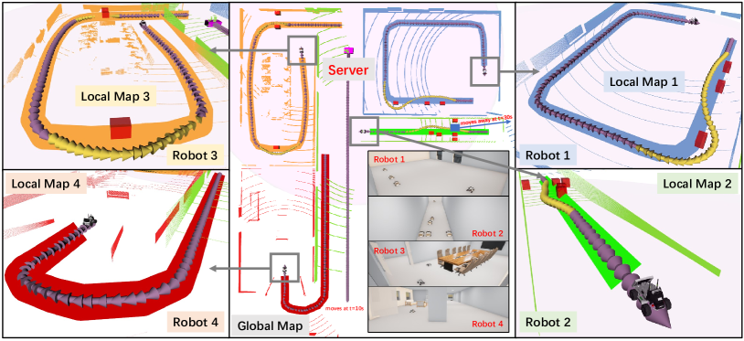
Figure 11: Multi-robot indoor scenario, where trajectories generated by the local and edge motion planners are marked in purple and yellow, respectively.

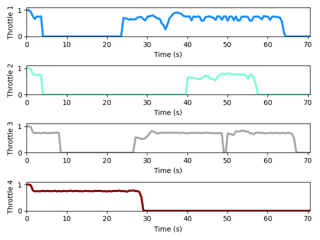
(a) Throttle commands

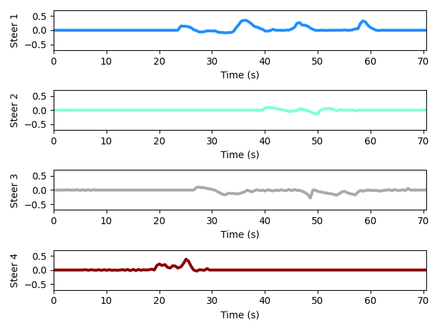
(b) Steer commands

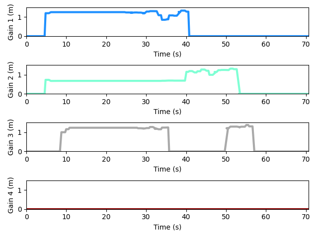
(c) Switching gains

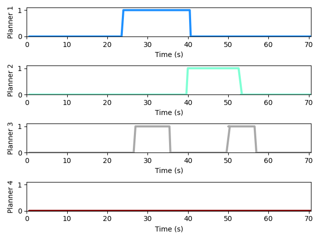
(d) Planner selections

Figure 12: The throttle commands, steer commands, switching gains, and planner selections of different robots.

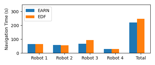
(a) Robot navigation time when $C_{\mathrm{th}}=240\,$ms

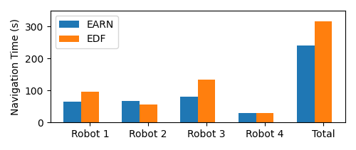
(b) Robot navigation time when $C_{\mathrm{th}}=160\,$ms

Figure 13: Comparison of the robot navigation time under different computation time constraints.

To verify the effectiveness of Algorithm 1, we implement EARN in a multi-robot indoor scenario shown in Fig. 11, where robot 1 navigates in an office room with its target path marked in blue, robot 2 navigates in a corridor with its target path marked in green, robot 3 navigates in a conference room with its target path marked in orange, and robot 4 navigates from a corridor to a lounge with its target path marked in red. The number of NPC robots, which are marked as red boxes, in local maps 1–4 are are $(|\mathcal{M}_{1}|,|\mathcal{M}_{2}|,|\mathcal{M}_{3}|,|\mathcal{M}_{4}|)=(3,6,3,0)$, respectively. The server (marked as a pink box) is assumed to be a Diablo wheel-legged robot with NVIDIA Orin NX. Each robot is simulated as an Ackerman steering car-like robot with their length, width, longitudinal wheelbase, and lateral wheelbase being $32.2\,$cm, $22.0\,$cm, $20.0\,$cm, and $17.5\,$cm, respectively, and the parameters $(\mathbf{A}_{k,t}$, $\mathbf{B}_{k,t}$, $\mathbf{c}_{k,t})$ in (1) are computed accordingly. The braking distance for planner $f_{L}$ is set to $d_{\mathrm{B}}=1.3$ m and the safe distance for planner $f_{E}$ is set to $d_{\mathrm{safe}}=0.1$ m. The length of prediction horizon is set to $H=20$, with the time step between consecutive motion planning frames being $0.25$ s. Using $H=20$ and the above $\{|\mathcal{M}_{k}|\}$, we have $(C_{1},C_{2},C_{3},C_{4})=(80,140,80,20)\,$ms. The total computation latency threshold is set to $C_{\mathrm{th}}=240\,$ms according to the operational speed in indoor environments. The execution time of PDD is assumed to be unacceptable when executed locally at the robot.

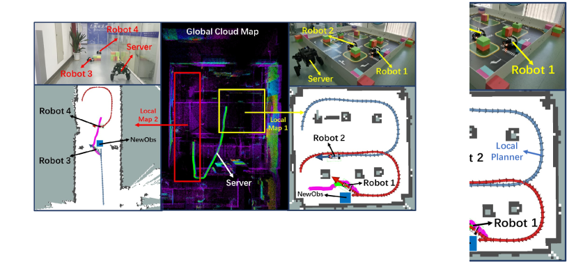
Figure 14: Real-world experiment, where robots 1–2 navigate in a sandbox and robots 3–4 navigate in a corridor.

The trajectories of $4$ robots under the proposed EARN are shown in Fig. 11, where the purple trajectories are generated by local motion planners (i.e., PF) and the yellow trajectories are generated by edge motion planners (i.e., PDD in Algorithm 2). The associated throttle commands, steer commands, switching gains $\{I_{k}\}$, and planner selections $\{\alpha_{k}\}$ are shown in Fig. 12a–12d. In particular, starting from $t=0\,$s, all robots adopt local motion planning and move at a speed of $0.55\,$m/s. Robot 4 encounters no obstacles along its target path; hence it keeps on moving using the local motion planner (i.e., the last subfigure of Fig. 12c–d) until reaching the goal at $t=29.64\,$s (i.e., the last subfigure of Fig. 12a–12b. In contrast, robots 1–3 stop in front of obstacles at $t=4.08\,$s, $3.88\,$s, and $8.52\,$s, respectively, as observed from Fig. 12a–12b. Consequently, the switching gains of robots 1 and 3 increase from $0$ to $1.2$. However, they cannot switch their planners immediately, since the edge server is now at the other side of the map and the communication latency between the server and robot 1 or 3 would be large. Note that the switching gain of robot 2 is only $0.67$, since the corridor is blocked by $4$ obstacles and the robot cannot pass the “traffic jam” even if it switches from local to edge planning.

At $t=10\,$s, the server starts to move upwards at a speed of $0.88\,$m/s, and collaborates with robots 1 and 3 for collision avoidance using edge motion planning with a speed of $0.67\,$m/s at $t=24.12\,$s and $t=27.12\,$s, respectively. After completing the collision avoidance actions, the switching gains of robots 1 and 3 become $0$ and the planners are switched back to local ones to save computation resources at the server. Furthermore, the switching gain of robot 2 increases from $0.67$ to $1.2$ at $t=40.08\,$s. This is because an NPC robot (marked as a blue box) in the corridor moves away at $t=30\,$s, leaving enough space for robot 2 to pass the traffic jam.

The average navigation time of EARN and EDF is provided in Fig. 13a. The navigation time of robots 1–4 with EARN is $64.80\,$s, $57.96\,$s, $67.68\,$s, and $29.64\,$s, respectively. The navigation time of robots 1–4 with EDF is $65.89\,$s, $56.40\,$s, $95.16\,$s, and $29.29\,$s, respectively. Compared to EDF, the total navigation time of EARN is reduced by $12.1\%$. This is because the EDF scheme is based on the expected task execution deadline, not on the low-level motion planning trajectories. As such, EDF fails to recognize the scenarios and traffic in real-time, leading to a potential resource-robot mismatch. For instance, in the considered indoor scenario, robots 2 and 4 are expected to finish their navigation tasks in a shorter time, since their target paths are shorter than other robots as seen from Fig. 11. This is also corroborated by Fig. 13a. Therefore, EDF selects robots 2 and 4 for edge motion planning, despite the fact that robot 2 gets stuck in the traffic jam and robot 4 has a small switching gain from the local to edge planner.

The navigation time of EARN and EDF under under $C_{\mathrm{th}}=160\,$ms is provided in Fig. 13b. Due to this tighter time constraint, the server cannot navigate multiple robots at the same time, and the waiting time for robots 1 and 3 becomes larger. Consequently, the robot navigation increases. However, the proposed EARN still outperforms EDF by a large margin.

V-E Real-World Testbed

Finally, to verify the hardware-software compatibility of EARN and its robustness against sensor and actuator uncertainties, we implement EARN in a real-world testbed consisting of a Diablo wheel-legged robot server and $4$ LIMO car-like robots. As shown in Fig. 14, we adopt the livox lidar and the fast-lio algorithm [27] to obtain a cm-level localization of the Diablo robot and the global cloud map of the indoor scenario. The trajectory of Diablo is marked as red-green-blue axes. The cloud map consists of two regions, where robots 1 and 2 navigate inside the sandbox (marked by a yellow box) and robots 3 and 4 navigate in the corridor (marked by a red box). All robots need to avoid collisions with the static environments as well as the cubes therein.

The trajectories of $4$ robots under the proposed EARN are shown at the left and right sides of Fig. 14, where the blue and red arrows are generated by local motion planners and the pink paths are generated by edge motion planners. It can be seen that robots 2 and 4 encounter no obstacles along their target path, and they execute the local motion planner without external assistance until reaching the goal at $t=25.45\,$s and $t=21.45\,$s, respectively. On the other hand, robots 1 and 3 encounter new obstacles (marked in blue boxes) and leverage planner switching in front of the blue boxes. Specifically, robot 1 and Diablo server collaboratively accomplish reverse and overtaking actions, so that the robot reaches the goal at $26.00\,$s. Robot 3 holds its position at the beginning and waits for connection with the server. At about $t=30\,$s, Diablo moves from the sandbox to the corridor and assists robot 3 for switching to edge motion planning at $t=64\,$s. With another $13.85\,$s, robot 3 reaches the goal. Please refer to our video for more details.

VI Conclusion

This paper proposed EARN to address the limited computation problem by empowering low-cost robots with proximal edge computing resources. EARN adopts a T-DMMP framework based on HMP and MPS, to opportunistically accelerate the trajectory computations while guaranteeing safety. CARLA simulations and real-world experiments have shown that EARN reduces the navigation time by $12.1\%$ and $46.7\%$ compared with EDF and PF schemes in indoor and outdoor scenarios, respectively. Furthermore, EARN increases the success rate by $53.1\%$ and $68.97\%$ compared with edge or local computing schemes.

References

- [1] K. M. Lynch and F. C. Park, Modern Robotics. Cambridge University Press, 2017.
- [2] W. Xia, W. Wang, and C. Gao, “Trajectory optimization with obstacles avoidance via strong duality equivalent and hp-pseudospectral sequential convex programming,” Optimal Control Applications and Methods, vol. 43, no. 2, pp. 566–587, 2022.
- [3] X. Zhang, A. Liniger, and F. Borrelli, “Optimization-based collision avoidance,” IEEE Transactions on Control Systems Technology, vol. 29, no. 3, pp. 972–983, May 2021.
- [4] Z. Wang, X. Zhou, and J. Wang, “Extremum-seeking-based adaptive model-free control and its application to automated vehicle path tracking,” IEEE/ASME Transactions on Mechatronics, vol. 27, no. 5, pp. 3874–3884, 2022.
- [5] Z. Han and et al., “An efficient spatial-temporal trajectory planner for autonomous vehicles in unstructured environments,” https://arxiv.org/abs/2208.13160, 2023.
- [6] F. Rey, Z. Pan, A. Hauswirth, and J. Lygeros, “Fully decentralized admm for coordination and collision avoidance,” in 2018 European Control Conference (ECC), 2018, pp. 825–830.
- [7] Z. Wang, Y. Zheng, S. E. Li, K. You, and K. Li, “Parallel optimal control for cooperative automation of large-scale connected vehicles via admm,” in 2018 International Conference on Intelligent Transportation Systems (ITSC), 2018, pp. 1633–1639.
- [8] R. Han, S. Wang, S. Wang, Z. Zhang, Q. Zhang, Y. C. Eldar, Q. Hao, and J. Pan, “RDA: An accelerated collision-free motion planner for autonomous navigation in cluttered environments,” IEEE Robotics and Automation Letters, no. 3, pp. 1715–1722, Mar. 2023.
- [9] Z. Huang, S. Shen, and J. Ma, “Decentralized ilqr for cooperative trajectory planning of connected autonomous vehicles via dual consensus admm,” IEEE Transactions on Intelligent Transportation Systems, pp. 1–8, 2023.
- [10] Y. Xiao, F. Codevilla, A. Gurram, O. Urfalioglu, and A. M. López, “Multimodal end-to-end autonomous driving,” IEEE Transactions on Intelligent Transportation Systems, vol. 23, no. 1, pp. 537–547, 2022.
- [11] Y. Pan, C.-A. Cheng, K. Saigol, K. Lee, X. Yan, E. A. Theodorou, and B. Boots, “Imitation learning for agile autonomous driving,” The International Journal of Robotics Research, vol. 39, no. 2-3, pp. 286–302, 2020.
- [12] W.-B. Kou, S. Wang, G. Zhu, B. Luo, Y. Chen, D. W. K. Ng, and Y.-C. Wu, “Communication resources constrained hierarchical federated learning for end-to-end autonomous driving,” in 2013 IEEE/RSJ International Conference on Intelligent Robots and Systems (IROS), 2023, pp. 1–8.
- [13] K. Goldberg, “Robots and the return to collaborative intelligence,” Nature Machine Intelligence, vol. 1, pp. 2–4, Jan. 2019.
- [14] A. K. Tanwani, R. Anand, J. E. Gonzalez, and K. Goldberg, “Rilaas: Robot inference and learning as a service,” IEEE Robotics and Automation Letters, vol. 5, no. 3, pp. 4423–4430, Jul. 2020.
- [15] S. Hayat, R. Jung, H. Hellwagner, C. Bettstetter, D. Emini, and D. Schnieders, “Edge computing in 5G for drone navigation: What to offload?” IEEE Robotics and Automation Letters, vol. 6, no. 2, pp. 2571–2578, 2021.
- [16] D. G. Syeda Tanjila Atik, Marco Brocanelli, “Are turn-by-turn navigation systems of regular vehicles ready for edge-assisted autonomous vehicles?” IEEE Transactions on Intelligent Transportation Systems, pp. 1–11, May 2023.
- [17] D. Liu, Z. Lyu, Q. Zou, X. Bian, M. Cong, and Y. Du, “Robotic navigation based on experiences and predictive map inspired by spatial cognition,” IEEE/ASME Transactions on Mechatronics, vol. 27, no. 6, pp. 4316–4326, 2022.
- [18] Q. Shi and M. Hong, “Penalty dual decomposition method for nonsmooth nonconvex optimization—Part I: Algorithms and convergence analysis,” IEEE Transactions on Signal Processing, vol. 68, pp. 4108–4122, Jun. 2020.
- [19] P. Huang, L. Zeng, X. Chen, K. Luo, Z. Zhou, and S. Yu, “Edge robotics: Edge-computing-accelerated multi-robot simultaneous localization and mapping,” IEEE Internet of Things Journal, vol. 9, no. 15, pp. 14 087–14 102, Aug. 2022.
- [20] J. Xu, H. Cao, Z. Yang, L. Shangguan, J. Zhang, X. He, and Y. Liu, “Swarmmap: Scaling up real-time collaborative visual slam at the edge,” in USENIX Symposium on Networked Systems Design and Implementation (NSDI 22), 2022, pp. 977–993.
- [21] J. Ichnowski and et al., “FogROS2: An adaptive platform for cloud and fog robotics using ros 2,” in 2023 IEEE International Conference on Robotics and Automation (ICRA), 2023.
- [22] K. Suiyz, M. Zhouy, D. Liuyz, M. Mayz, D. Peiyz, Y. Zhaoyz, Z. Liy, and T. Moscibroda, “Characterizing and improving wifi latency in large-scale operational networks,” in MobiSys’16, June 2016.
- [23] S. Zhang, S. Wang, S. Yu, J. Yu, and M. Wen, “Collision avoidance predictive motion planning based on integrated perception and V2V communication,” IEEE Transactions on Intelligent Transportation Systems, vol. 23, no. 7, pp. 9640–9653, July 2022.
- [24] A. Dosovitskiy, G. Ros, F. Codevilla, A. Lopez, and V. Koltun, “Carla: An open urban driving simulator,” in Conference on Robot Learning, vol. 78, 2017, pp. 1–16.
- [25] CARLA-ROS-Bridge: https://github.com/carla-simulator/ros-bridge.
- [26] J. Wehbeh, S. Rahman, and I. Sharf, “Distributed model predictive control for uavs collaborative payload transport,” in IEEE/RSJ International Conference on Intelligent Robots and Systems (IROS), Las Vegas, Feb. 2021.
- [27] W. Xu, Y. Cai, D. He, J. Lin, and F. Zhang, “Fast-lio2: Fast direct lidar-inertial odometry,” IEEE Transactions on Robotics, vol. 38, no. 4, pp. 2053–2073, Aug. 2022.