Probing Iron in Earth’s Core With Molecular-Spin Dynamics

Abstract

Dynamic compression of iron to Earth-core conditions is one of the few ways to gather important elastic and transport properties needed to uncover key mechanisms surrounding the geodynamo effect. Herein a new machine-learned ab-initio derived molecular-spin dynamics (MSD) methodology with explicit treatment for longitudinal spin-fluctuations is utilized to probe the dynamic phase-diagram of iron. This framework uniquely enables an accurate resolution of the phase-transition kinetics and Earth-core elastic properties, as highlighted by compressional wave velocity and adiabatic bulk moduli measurements. In addition, a unique coupling of MSD with time-dependent density functional theory enables gauging electronic transport properties, critically important for resolving geodynamo dynamics.

Introduction  —  Iron, Earth’s most abundant element by mass, unveils intricate and multifaceted behaviors under extreme temperatures and pressures. For millennia, iron has been an integral part of human civilization, with approximately 90% of global metal refining dedicated to its myriad of applications, spanning from kitchen utensils and structural building components, to microscopic drug delivery systems Dagdelen et al. (2023); Denmark et al. (2016). The significance of iron transcends its uses on and above the terrestrial surface. Earth’s core, predominantly constituted of iron, assumes a central role in the planet’s geophysical and geochemical processes Cole and Woolfson (2002). At pressures approaching 350 GPa and temperatures surpassing 6000 K, the flow of iron in the planet’s core acts as the source of Earth’s magnetic field, shielding our planet from detrimental solar radiation while exerting influence over plate tectonics and mantle convection. Hence, it is not an overstatement that iron is critical for life on Earth. Yet still, the precise mechanisms responsible for upholding Earth’s magnetic fields remain unclear Landeau et al. (2022). The prevailing theory posits a dynamo mechanism within the outer core, where the convective motion of molten iron generates electrical currents, giving rise to the magnetic field we observe Frazer (1973); Labrosse (2003); Stacey and Loper (2007). Unraveling the geodynamo mechanism crucially depends on the underlying material properties. Understanding the phase diagram of iron, especially its melting line Kraus et al. (2022), and transport properties, such as electrical and thermal conductivity, across a wide spectrum of temperatures and pressures, are pivotal in this pursuit Pozzo et al. (2012).

Numerous experimental endeavors have significantly enhanced our comprehension of the iron phase diagram. Early measurements employed both compressive Bancroft et al. (1956) and shock Anderson (1986) waves to investigate polymorphic phases at low pressure and the phase diagram up to Earth-core conditions. Recent measurements Takahashi and Bassett (1964); Mathon et al. (2004); Dewaele et al. (2006); Kuwayama et al. (2020a); Hwang et al. (2020a); White et al. (2020); Grant et al. (2021), utilizing short pulse optical lasers, laser-driven shocks, and dynamic compression techniques, have further expanded our knowledge of iron’s phase diagram. Although fewer in number, investigations of iron’s transport properties have been conducted using DAC Gomi et al. (2013); Ohta et al. (2016); Konôpková et al. (2016); Ohta et al. (2023), wire-heating Konôpková et al. (2016); Beutl et al. (1994), and both static and dynamic shock-compression Keeler and Mitchell (1969); Gathers (1983, 1986). Remarkably, experiments involving laser-heated DAC Ohta et al. (2016); Konôpková et al. (2016) have ignited controversy in measuring electronic transport properties at Earth-core conditions Dobson (2016). These indispensable experimental efforts demand significant effort to achieve the necessary accuracy, and therefore motivate computational efforts to fill in gaps in transport properties throughout the phase diagram.

Figure 1: a) Hugoniot states ($u_{p}$, P) in shocked iron for both FM and LSF cases. The top inset is the pressure difference ($\Delta$) between FM-LSF calculations, with a common axis along $u_{p}$. b) Hugoniot states ($u_{p}$, $u_{s}$) for an initial temperature of 300$K$. Upper panel captures $\Delta=u_{s}^{FM}-u_{s}^{LSF}$. For $u_{p}\leq$ 1.2 km/s both elastic and plastic wavefronts are separated spatially, above which a single wave is observed. c) MSD snapshots from LSF simulations at different piston speeds, color indicating phase, and grayscale arrows for spin vectors where present (see magnetic moment legend). At $u_{p}\simeq 0.6$ km/s a clear BCC-HCP transition is detected where magnetic moments for HCP atoms decrease rapidly with pressure, see inset for clarity. The onset of melting occurs $u_{p}\geq 2.8$ km/s, lower close-up image shows few atoms retain their magnetic moments in this molten state.

Previous simulation efforts, employing various levels of theory, have extensively explored the iron phase diagram, encompassing its polymorphs and phases at high pressure and temperature Hasegawa and Pettifor (1983); Pourovskii (2019); Kruglov et al. (2023). Furthermore, there has been a growing emphasis on the development of increasingly accurate equation of state models Zhang et al. (2010); Sha and Cohen (2010); Dorogokupets et al. (2017). More recently, classical molecular dynamics (MD) simulations Alder and Wainwright (1959), based on the parameterization of a Born-Oppenheimer potential energy surface (BO-PES) Rapaport (2004) using machine-learning techniques, have emerged as the state of the art in atomistic modeling. A substantial number of highly precise machine-learned interatomic potentials have been built from ab-initio calculations Kohn and Sham (1965); Behler and Parrinello (2007); Huan et al. (2017); Smith et al. (2017); Zhang et al. (2018); Bartók et al. (2010); Jaramillo-Botero et al. (2014); Lubbers et al. (2018); Schütt et al. (2018); Thompson et al. (2015) with various model forms and feature sets. While invaluable for large-scale investigations of material properties Li et al. (2020a); Cusentino et al. (2020), these new potentials have primarily been confined to non-magnetic phases, consequently making inaccurate predictions of simple properties like heat capacity Dragoni et al. (2018). To resolve this, recent efforts have incorporated atomic spin dynamics into MD simulations Ma et al. (2008); Tranchida et al. (2018). Although early models provided qualitative agreement with experimental results Ma et al. (2016); Dos Santos et al. (2020); Zhou et al. (2020) via embedded-atom-method potentials Ma and Dudarev (2020), recent advancements have successfully constructed magneto-elastic potentials for coupled molecular-spin dynamics (MSD) simulations, achieving accuracies similar to the underlying first-principles methods Nikolov et al. (2021, 2022); Nieves et al. (2022); Nikolov et al. (2023); Rohskopf et al. (2023).

In this letter, building on prior spin-dynamical efforts Ruban et al. (2007); Ma and Dudarev (2012); Gambino et al. (2020), we incorporate longitudinal spin fluctuations (LSFs) into our MSD framework and demonstrate this necessary adaptation for the behavior of iron up to Earth-core conditions. To resolve magnon-phonon interactions within our computationally efficient MSD framework, a quantum-accurate ML potential is constructed that properly partitions magnetic/non-magnetic contributions to the BO-PES Nikolov et al. (2021). Due to experimental parallels, to study Earth-core states of matter, we simulate the iron single-crystalline Hugoniot curves up to Earth-core conditions, where changes in initial preheat temperature permit mapping out a large part of the structural polymorphs and liquidus. One of the unique benefits of the current MSD approach is the access to orders of magnitude larger, compared to DFT methods, temporal/spatial domains which minimizes the barrier to providing fundamental transport properties for geophysical models. To illustrate this capability, elastic properties of iron for a 5882$K$ isotherm are measured up to roughly 300 GPa, enabling direct comparison to preliminary reference Earth model (PREM) measurements for compressional "P-wave" velocities and adiabatic bulk modulus ($B$). Additional transport property measurements are enabled by a top-down multiscale modeling approach wherein from large MSD simulations representative structures can be isolated and used for detailed time-dependent density functional theory (TDDFT) simulations Ramakrishna et al. (2023a, b). Electrical-resistivity measurements are carried out in the range of 2000-4000$K$ at both 140 and 212 $GPa$, highlighting the impact of LSFs and showing good agreement with experimental measurements by Ohta and Zhang et al. Ohta et al. (2023, 2016); Zhang et al. (2020). These demonstrations usher in new computational approaches for magnetic materials that have been absent, or under-resolved, for high-energy density states of matter.

Results and Discussion  —  The iron phase diagram Hasegawa and Pettifor (1983); Anderson (1986); Pourovskii (2019); Hwang et al. (2020a); White et al. (2020); Kruglov et al. (2023) and its equation of state Garai et al. (2011); Andrews (1973); Dorogokupets et al. (2017); Anderson (1986); Pourovskii (2019); Zhang et al. (2010); Dewaele et al. (2006); Sha and Cohen (2010); Grant et al. (2021); Kuwayama et al. (2020a); González-Cataldo and Militzer (2023) have been thoroughly investigated in recent decades. Within these efforts the behavior of iron, particularly across large regions of temperature-pressure space has been difficult to pin down, partly due to the variety of phases iron can take on ($\alpha$, $\gamma$, $\epsilon$, $\delta$, liquid) and the underlying magnetic character for some of these phases. The ability to accurately resolve large portions of the iron phase diagram, in an atomistic setting, where one can predict, free from finite size/time restrictions the underlying grain structure, phase stability, transient (shock) kinetics, and transport properties (viscosity, electrical/thermal conductivity, self-diffusion, etc.) is of particular importance due to the underlying implications that these measurements have in the calculation of Earth-core Anderson (1986); Mao et al. (1967); Anzellini et al. (2013); Kraus et al. (2022) properties.

To this end, our simulation efforts begin by focusing on the construction of the iron phase diagram that includes a prediction of high-pressure/temperature metastable phases. An efficient means to sample large areas in $P$/$T$ phase space is to shock compress (Fig. 1) a sample of varying initial (preheat) temperatures, where each piston impact velocity ($u_{p}$) generates a locus of Hugoniot points. Herein a key simulation capability advancement Luu et al. (2020); Kadau et al. (2007) is the proper partitioning of magnetic and non-magnetic contributions to the potential energy surface, enabling a higher fidelity resolution of the transient shock dynamics. Longitudinal spin fluctuations may have previously been regarded as having a subtle effect on the ion dynamics, but as noted in Fig. 1 appreciable differences between the fixed-moment (FM - constant magnetic moment) and LSF cases can be seen. Namely, the top panels of Fig. 1.a-b) compute the difference in pressure and shock velocity, respectively, where up to 25 $GPa$ and 1 $km/s$ differences can be seen for the shock simulations with the highest preheat.

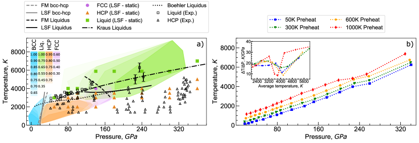
Figure 2: a) Dynamic phase diagram for iron with MSD-LSF. Observed phases (colored areas) consist of four (50$K$, 300$K$, 600$K$, and 1000$K$) preheat temperatures Nguyen and Holmes (2004), which have been categorized according as light-blue - BCC, purple - FCC, orange - HCP, green - liquid. The liquid and HCP experimental data points are compiled from the works of Morard, Kuwayama, Anzellini, Jeffrey, Brown, Yoo, and Tateno et al. Morard et al. (2014); Kuwayama et al. (2020b); Tateno et al. (2010); Nguyen and Holmes (2004); Yoo et al. (1995); Brown and McQueen (1986); Anzellini et al. (2013). The predicted melt line from LSF simulations is in far better agreement with Kraus/Boehler Kraus et al. (2022); Boehler (1993) lines than MSD-FM. b) Temperature vs. Pressure Hugoniot curves for the four different preheat temperatures. The inset shows how the numerical derivative of each curve varies with temperature, highlighting the predicted melting transition.

The well-characterized Kadau et al. (2007); Jensen et al. (2009); Hwang et al. (2020b); Luu et al. (2020) split elastic/plastic wave structure is recovered at $u_{p}<1.2$ $km/s$, with the $\alpha-\epsilon$ transition occurring at approx. $0.6$ $km/s$ ($\approx 16$ $GPa$), see top image of Fig. 1.c. In the MSD-LSF simulations (Fig. 1.a,c), transitioning into the HCP phase brings about a strong decrease in the atomic spin magnitude which lowers the exchange/Landau contributions, resulting in lower pressure Hugoniot states. An in-depth overview of the LSF scheme and the corresponding strain-phase-magnetic-moment relationships can be found in the SI. Interestingly, both FM and LSF shock data predict a meta-stable FCC phase near the liquidus, $\sim 160$ $GPa$ ($u_{p}\simeq 2.2$ $km/s$). The value in phase predictions from shock-compressed samples is this direct capture of meta-stability, which can help resolve differences in transport properties reported in the literature Ohta et al. (2016); Konôpková et al. (2016).

Utilizing the MSD shock data here we construct a dynamic phase diagram by sampling 10 $nm$ thick slices of material behind the shock front at 0.5 $ps$ intervals to identify $P$, $T$, and phases present. This data is collected in Fig. 2.a. Color-shaded areas indicate MSD-LSF predicted phase fractions for BCC/HCP/FCC/Liquid (blue/orange/purple/green) phases, where overlapping regions indicate metastable mixed phases. Phase boundaries demarking $\alpha$-$\epsilon$ and liquidus for both LSF and FM are shown as lines and are constructed via support vector classification Deffrennes et al. (2022); Maulik and Chakraborty (2017). Additional liquidus lines from Boehler Boehler (1993) and Kraus Kraus et al. (2022) show much better agreement with LSF predictions than FM, highlighting the need for proper accounting of magnetic effects at high pressure and temperature conditions. Likewise for the BCC/HCP transition curves a difference between the FM/LSF case is observed, whereas for the LSF simulations, the BCC/HCP transition curve is shown to be less temperature sensitive.

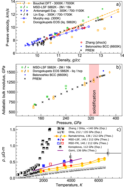
Figure 3: a) Literature data Bouchet et al. (2022); Antonangeli et al. (2012); Lin et al. (2005); Murphy et al. (2013) and predicted compressional wave MSD-LSF data (green markers) for liquid iron at $\sim$5882K. Finite-size effects are resolved with MSD, as exemplified by differences between 2M and 16k atom count simulations. b) Pressure-dependent adiabatic bulk modulus as compared to PREM, for 5882$K$ MSD-LSF isotherm, and 5882$K$ isotherms from Dorogokupets EOS model Dorogokupets et al. (2017). A lone data point for the BCC phase is included from Belonoshko et al. to highlight the liquidus crossing near 320GPa Belonoshko et al. (2022). c) Temperature-dependent electrical resistivity for pressures close to 140 GPa and 212 GPa from experiment and theory. DAC measurements were reported by Ohta et al. Ohta et al. (2016, 2023), Zhang et al. Zhang et al. (2020) and by Konôpková et al. Konôpková et al. (2016). Our calculations of the electrical conductivity using LSF/FM (red/blue stars and squares) are compared with previously reported calculations Gomi et al. (2013); Ramakrishna et al. (2023a).

Overlaying the dynamic phase diagram are static LSF-MSD calculations, filled symbols, which were performed using a large $2\cdot 10^{6}$ atom simulation cell held at the designated $P/T$ for 200 $ps$. The static calculations here importantly fill in regions that are not well resolved within the dynamic phase diagram and agree well with experimental DAC results Kuwayama et al. (2020b); Morard et al. (2014); Denoeud et al. (2016); Yoo et al. (1995); Morard et al. (2018); Anzellini et al. (2013); Tateno et al. (2010). Notably within the static melt measurements, we do observe a metastable BCC transition (see Figure 5 in SI) which occurs right before the pair correlation function of the sample assumes the standard liquid profile, such metastability has been previously discussed by Bouchet and Belonoshko Belonoshko et al. (2021, 2022); Bouchet et al. (2013). Within the SI we provide a snapshot that shows how melting is initiated from the metastable BCC state.

An additional estimate of the liquidus, independent of the structure detection algorithm, is provided in Fig. 2.b, which illustrates the LSF Hugoniot curves for each initial temperature used to construct our dynamic phase diagram. The inflection in the P, T curve is indicative of a phase transition. The inset in Fig. 2.b thus highlights the observed melt-transitions by showing how the derivatives of each curve vary with temperature. Based on this data the estimated melting point for a 300$K$ preheat is $[239\mp 14GPa,\ 4182\mp 123K]$. These results are in agreement with the previous laser multi-shock study by Ping et al. which arrive at approx. $[250\mp 30GPa,\ 4950\mp 1050K]$ Ping et al. (2013). Meanwhile, sound velocity experiments by Nguyen et al. find a melting point of approx $[226GPa,\ 5000\mp 500K]$, which in terms of temperature, is a little bit higher than the current estimates. This agreement with the few available experimental studies gives support to the accuracy of the computational tools developed herein.

Elastic Properties — Having constructed our dynamic MSD-LSF phase diagram, we now turn to measurements of elastic and transport properties relevant to the proposed dynamo effect of Earth’s core. Measurements for the compressional $P$-wave velocities and adiabatic bulk moduli for a 5882 $K$ isotherm within the pressure range of 140-300 $GPa$ were carried out for small ($1.6\cdot 10^{4}$ atoms) and large ($2.0\cdot 10^{6}$ atoms) liquid samples. This data is displayed in Fig. 3 along with available DFT, experimental, EOS, and PREM predictions. Note differences in temperature indicated in the legends as this will dictate the (meta-)stable phase present in the measurement. At the largest densities, we observe significant differences between the small and large MSD simulation cells which arise due to the fact that the large cells are all fully melted. In contrast, the smaller geometries retain a strong signal of BCC above 200 $GPa$ (additional details in SI). The current findings thus support the existence of a high-pressure BCC phase, however, it is unclear whether this phase is a fully stable state or just a transient state that is encountered on the path to melting. While the current calculations point to the latter, a fully stable high-pressure BCC region may exist within an unresolved region of pressure/temperature space. Importantly, this has been hypothesized by Belonoshko et al. within their recent works Belonoshko et al. (2022, 2021, 2017), as a potential way of explaining the anisotropy of Earth-core seismic wave measurements. Fig. 3.b captures the current MSD-LSF results for the adiabatic bulk modulus and includes a corresponding comparison with PREM and EOS data for pure iron Dorogokupets et al. (2017). Again finite-size effects are observed between large and small simulation cells above 200 $GPa$.

In general, we find that the largest deviations from the PREM are $\sim 10\%$, showing the MSD-LSF model has great transferability over a large range of temperatures and pressures, something previously unachievable using standard MD approaches  Rosenbrock et al. (2021). Note that experimental seismic measurements indicate the presence of lighter elements within the iron lattice Poirier (1994). Recent studies have revealed that these light elements can impact elastic properties and melting temperatures at Earth-core pressures He et al. (2022); Li et al. (2020b); Hirose et al. (2021); Umemoto and Hirose (2020). Thus an overly close agreement between PREM and pure iron results should not be anticipated. Solid BCC predictions from Belonoshko Belonoshko et al. (2022) are also included in Fig. 3.b, which albeit at a slightly higher temperature, agrees well with the trend in the MSD-LSF data. The red highlighted region here denotes where solidification is expected for the 5882 $K$ isotherm.

Transport Properties — Lastly, we leverage the computational efficiency of MSD-LSF for ensemble sampling of structures which in turn are returned to ab-initio codes for transport property measurements. The experiments with laser-heated DAC Ohta et al. (2016); Konôpková et al. (2016) have led to a notable controversy in the measurement of electronic transport properties in iron at the core-mantle boundary (CMB) and Earth-core conditions Dobson (2016); Lobanov and Geballe (2022). Ohta et al. Ohta et al. (2016) infer a thermal conductivity of 226 Wm^-1K^-1 by measuring the electrical resistance of iron wires and converting it into a thermal conductivity using the Wiedemann-Franz law Franz and Wiedemann (1853). Alternatively, Konôpková et al. Konôpková et al. (2016) measured the thermal diffusion rate for heat transferred between the ends of solid iron samples, inferring a thermal conductivity of 33 Wm^-1K^-1 from the agreement with a finite-element model. The discrepancy in these measurements has deep implications for predicting the age of the Earth Dobson (2016). Since the uncertainty in the electrical conductivity, both from experiment and theory is so high, reliable knowledge about the fundamental processes generating Earth’s magnetic field is also lacking. Due to the disagreement among existing experimental data, computational modeling is indispensable in supporting current and future efforts probing these properties Berrada and Secco (2021).

Fig. 3.c shows the electrical resistivity and its temperature dependence at a fixed pressure (P=140 GPa and P=212 GPa). Additional details regarding the simulation parameters can be found in the SI. Structures sampled from LSF and FM MSD simulations are indicated by red/blue stars and squares respectively, highlighting the importance of proper magnetic treatment leading to these high-energy density states. The striking feature is that the predicted electrical resistivity agrees well with the recent measurements of Ohta et al. Ohta et al. (2023), particularly at 135 GPa and $\sim$4000 K as well as the earlier DAC measurements by Ohta and Zhang et al. at 2000 K compared to other ab-initio models Gomi et al. (2013); Ramakrishna et al. (2023a). The influence of LSF on the ionic configurations results in a slightly higher resistivity at higher temperatures, especially between 3000 K to 4000 K in agreement with Ohta et al.

Conclusion  —  The present work illustrates a promising simulation capability that incorporates an explicit treatment for magnetic exchange interactions and LSFs into efficient machine-learned interatomic potentials to resolve structural, mechanical, and transport properties of iron at high temperatures and pressures. Far-reaching effects of LSFs on key geophysical material properties were demonstrated, in particular phase stability in shock-compressed systems. The prediction of a metastable FCC phase under shock near 160 GPa will test new experimental X-ray diagnostics at state-of-the-art light source facilities. Meanwhile, our static liquid calculations hint at a high-pressure BCC phase which could explain the anisotropic character of PREM seismic wave velocities. Recent studies have highlighted that a metastable inner-core BCC phase can be stabilized by the presence of light elements Wu and Wang (2022); Godwal et al. (2015), and as such future work will leverage our unique MSD-TDDFT approach to determine the impact of this high-pressure BCC phase on electrical resistivities in Earth’s inner core Wu and Wang (2022); He et al. (2022); Godwal et al. (2015).

Acknowledgement  —  This article has been authored by an employee of National Technology & Engineering Solutions of Sandia, LLC under Contract No. DE-NA0003525 with the U.S. Department of Energy (DOE). The employee owns all right, title and interest in and to the article and is solely responsible for its contents. The United States Government retains and the publisher, by accepting the article for publication, acknowledges that the United States Government retains a non-exclusive, paid-up, irrevocable, world-wide license to publish or reproduce the published form of this article or allow others to do so, for United States Government purposes. The DOE will provide public access to these results of federally sponsored research in accordance with the DOE Public Access Plan . KR and AC were supported by the Center for Advanced Systems Understanding (CASUS) which is financed by Germany’s Federal Ministry of Education and Research (BMBF) and by the Saxon state government out of the State budget approved by the Saxon State Parliament. Some computations were performed on a Bull Cluster at the Center for Information Services and High-Performance Computing (ZIH) at Technische Universität Dresden, on the cluster Hemera at Helmholtz-Zentrum Dresden-Rossendorf (HZDR). We want to thank the ZIH for its support and generous allocations of computer time.

References

- Dagdelen et al. (2023) S. Dagdelen, M. Mackiewicz, M. Osial, E. Waleka-Bargiel, J. Romanski, P. Krysinski, and M. Karbarz, Journal of Materials Science 58, 4094 (2023).
- Denmark et al. (2016) D. Denmark, J. Bradley, D. Mukherjee, J. Alonso, S. Shakespeare, N. Bernal, M. Phan, H. Srikanth, S. Witanachchi, and P. Mukherjee, RSC advances 6, 5641 (2016).
- Cole and Woolfson (2002) G. Cole and M. Woolfson, Planetary Science: The Science of Planets Around Stars (Taylor & Francis, 2002), ISBN 9780750308151.
- Landeau et al. (2022) M. Landeau, A. Fournier, H.-C. Nataf, D. Cébron, and N. Schaeffer, Nature Reviews Earth & Environment 3, 255 (2022), URL https://doi.org/10.1038%2Fs43017-022-00264-1.
- Frazer (1973) M. Frazer, Geophysical Journal International 34, 193 (1973).
- Labrosse (2003) S. Labrosse, Physics of the Earth and Planetary Interiors 140, 127 (2003).
- Stacey and Loper (2007) F. Stacey and D. Loper, Physics of the Earth and Planetary Interiors 161, 13 (2007).
- Kraus et al. (2022) R. G. Kraus, R. J. Hemley, S. J. Ali, J. L. Belof, L. X. Benedict, J. Bernier, D. Braun, R. Cohen, G. W. Collins, F. Coppari, et al., Science 375, 202 (2022).
- Pozzo et al. (2012) M. Pozzo, C. Davies, D. Gubbins, and D. Alfè, Nature 485, 355 (2012), URL https://doi.org/10.1038%2Fnature11031.
- Bancroft et al. (1956) D. Bancroft, E. L. Peterson, and S. Minshall, Journal of Applied Physics 27, 291 (1956).
- Anderson (1986) O. L. Anderson, Geophysical Journal International 84, 561 (1986).
- Takahashi and Bassett (1964) T. Takahashi and W. A. Bassett, Science 145, 483 (1964).
- Mathon et al. (2004) O. Mathon, F. Baudelet, J. P. Itié, A. Polian, M. d’Astuto, J. C. Chervin, and S. Pascarelli, Phys. Rev. Lett. 93, 255503 (2004), URL https://link.aps.org/doi/10.1103/PhysRevLett.93.255503.
- Dewaele et al. (2006) A. Dewaele, P. Loubeyre, F. Occelli, M. Mezouar, P. I. Dorogokupets, and M. Torrent, Phys. Rev. Lett. 97, 215504 (2006), URL https://link.aps.org/doi/10.1103/PhysRevLett.97.215504.
- Kuwayama et al. (2020a) Y. Kuwayama, G. Morard, Y. Nakajima, K. Hirose, A. Q. R. Baron, S. I. Kawaguchi, T. Tsuchiya, D. Ishikawa, N. Hirao, and Y. Ohishi, Phys. Rev. Lett. 124, 165701 (2020a), URL https://link.aps.org/doi/10.1103/PhysRevLett.124.165701.
- Hwang et al. (2020a) H. Hwang, E. Galtier, H. Cynn, I. Eom, S. Chun, Y. Bang, G. Hwang, J. Choi, T. Kim, M. Kong, et al., Science Advances 6, eaaz5132 (2020a).
- White et al. (2020) S. White, B. Kettle, J. Vorberger, C. Lewis, S. Glenzer, E. Gamboa, B. Nagler, F. Tavella, H. Lee, C. Murphy, et al., Physical Review Research 2, 033366 (2020).
- Grant et al. (2021) S. Grant, T. Ao, C. Seagle, A. Porwitzky, J.-P. Davis, K. Cochrane, D. Dolan, J.-F. Lin, T. Ditmire, and A. Bernstein, Journal of Geophysical Research: Solid Earth 126, e2020JB020008 (2021).
- Gomi et al. (2013) H. Gomi, K. Ohta, K. Hirose, S. Labrosse, R. Caracas, M. J. Verstraete, and J. W. Hernlund, Physics of the Earth and Planetary Interiors 224, 88 (2013).
- Ohta et al. (2016) K. Ohta, Y. Kuwayama, K. Hirose, K. Shimizu, and Y. Ohishi, Nature 534, 95 (2016).
- Konôpková et al. (2016) Z. Konôpková, R. S. McWilliams, N. Gómez-Pérez, and A. F. Goncharov, Nature 534, 99 (2016).
- Ohta et al. (2023) K. Ohta, S. Suehiro, S. I. Kawaguchi, Y. Okuda, T. Wakamatsu, K. Hirose, Y. Ohishi, M. Kodama, S. Hirai, and S. Azuma, Phys. Rev. Lett. 130, 266301 (2023), URL https://link.aps.org/doi/10.1103/PhysRevLett.130.266301.
- Beutl et al. (1994) M. Beutl, G. Pottlacher, and H. Jäger, International journal of thermophysics 15, 1323 (1994).
- Keeler and Mitchell (1969) R. Keeler and A. Mitchell, Solid State Communications 7, 271 (1969).
- Gathers (1983) G. Gathers, International journal of Thermophysics 4, 209 (1983).
- Gathers (1986) G. Gathers, Reports on Progress in Physics 49, 341 (1986).
- Dobson (2016) D. Dobson, Nature 534, 45 (2016).
- Hasegawa and Pettifor (1983) H. Hasegawa and D. G. Pettifor, Phys. Rev. Lett. 50, 130 (1983), URL https://link.aps.org/doi/10.1103/PhysRevLett.50.130.
- Pourovskii (2019) L. V. Pourovskii, Journal of Physics: Condensed Matter 31, 373001 (2019).
- Kruglov et al. (2023) I. A. Kruglov, A. V. Yanilkin, Y. Propad, A. B. Mazitov, P. Rachitskii, and A. R. Oganov, npj Computational Materials 9, 197 (2023).
- Zhang et al. (2010) H. Zhang, S. Lu, M. P. J. Punkkinen, Q.-M. Hu, B. Johansson, and L. Vitos, Physical Review B 82, 132409 (2010).
- Sha and Cohen (2010) X. Sha and R. Cohen, Physical Review B 81, 094105 (2010).
- Dorogokupets et al. (2017) P. Dorogokupets, A. Dymshits, K. Litasov, and T. Sokolova, Scientific reports 7, 1 (2017).
- Alder and Wainwright (1959) B. J. Alder and T. E. Wainwright, The Journal of Chemical Physics 31, 459 (1959).
- Rapaport (2004) D. C. Rapaport, The art of molecular dynamics simulation (Cambridge university press, 2004).
- Kohn and Sham (1965) W. Kohn and L. J. Sham, Phys. Rev. 140, A1133 (1965).
- Behler and Parrinello (2007) J. Behler and M. Parrinello, Phys. Rev. Lett. 98, 146401 (2007), URL https://link.aps.org/doi/10.1103/PhysRevLett.98.146401.
- Huan et al. (2017) T. D. Huan, R. Batra, J. Chapman, S. Krishnan, L. Chen, and R. Ramprasad, npj Computational Materials 3 (2017), ISSN 2057-3960.
- Smith et al. (2017) J. S. Smith, O. Isayev, and A. E. Roitberg, Chem. Sci. 8, 3192 (2017), URL http://dx.doi.org/10.1039/C6SC05720A.
- Zhang et al. (2018) L. Zhang, J. Han, H. Wang, R. Car, and W. E, Phys. Rev. Lett. 120, 143001 (2018).
- Bartók et al. (2010) A. P. Bartók, M. C. Payne, R. Kondor, and G. Csányi, Phys. Rev. Lett. 104, 136403 (2010).
- Jaramillo-Botero et al. (2014) A. Jaramillo-Botero, S. Naserifar, and W. A. Goddard, Journal of Chemical Theory and Computation 10, 1426 (2014).
- Lubbers et al. (2018) N. Lubbers, J. S. Smith, and K. Barros, The Journal of Chemical Physics 148, 241715 (2018).
- Schütt et al. (2018) K. T. Schütt, H. E. Sauceda, P.-J. Kindermans, A. Tkatchenko, and K.-R. Müller, The Journal of Chemical Physics 148, 241722 (2018).
- Thompson et al. (2015) A. P. Thompson, L. P. Swiler, C. R. Trott, S. M. Foiles, and G. J. Tucker, Journal of Computational Physics 285, 316 (2015), ISSN 0021-9991.
- Li et al. (2020a) X.-G. Li, C. Chen, H. Zheng, Y. Zuo, and S. P. Ong, npj Computational Materials 6, 1 (2020a).
- Cusentino et al. (2020) M. Cusentino, M. Wood, and A. Thompson, Nuclear Fusion 60, 126018 (2020).
- Dragoni et al. (2018) D. Dragoni, T. D. Daff, G. Csányi, and N. Marzari, Physical Review Materials 2, 013808 (2018).
- Ma et al. (2008) P.-W. Ma, C. H. Woo, and S. L. Dudarev, Phys. Rev. B 78, 024434 (2008), URL https://link.aps.org/doi/10.1103/PhysRevB.78.024434.
- Tranchida et al. (2018) J. Tranchida, S. Plimpton, P. Thibaudeau, and A. P. Thompson, Journal of Computational Physics 372, 406 (2018).
- Ma et al. (2016) P.-W. Ma, S. Dudarev, and C. Woo, Computer Physics Communications 207, 350 (2016).
- Dos Santos et al. (2020) G. Dos Santos, R. Aparicio, D. Linares, E. Miranda, J. Tranchida, G. Pastor, and E. Bringa, Physical Review B 102, 184426 (2020).
- Zhou et al. (2020) Y. Zhou, J. Tranchida, Y. Ge, J. Murthy, and T. S. Fisher, Physical Review B 101, 224303 (2020).
- Ma and Dudarev (2020) P.-W. Ma and S. Dudarev, Handbook of Materials Modeling: Methods: Theory and Modeling pp. 1017–1035 (2020).
- Nikolov et al. (2021) S. Nikolov, M. A. Wood, A. Cangi, J.-B. Maillet, M.-C. Marinica, A. P. Thompson, M. P. Desjarlais, and J. Tranchida, npj Computational Materials 7 (2021), URL https://doi.org/10.1038%2Fs41524-021-00617-2.
- Nikolov et al. (2022) S. Nikolov, J. Tranchida, K. Ramakrishna, M. Lokamani, A. Cangi, and M. A. Wood, Journal of Materials Science 57, 10535 (2022), URL https://doi.org/10.1007%2Fs10853-021-06865-3.
- Nieves et al. (2022) P. Nieves, J. Tranchida, S. Nikolov, A. Fraile, and D. Legut, Physical Review B 105, 134430 (2022).
- Nikolov et al. (2023) S. Nikolov, P. Nieves, A. Thompson, M. Wood, and J. Tranchida, Physical Review B 107, 094426 (2023).
- Rohskopf et al. (2023) A. Rohskopf, C. Sievers, N. Lubbers, M. Cusentino, J. Goff, J. Janssen, M. McCarthy, D. M. O. de Zapiain, S. Nikolov, K. Sargsyan, et al., Journal of Open Source Software 8, 5118 (2023).
- Ruban et al. (2007) A. V. Ruban, S. Khmelevskyi, P. Mohn, and B. Johansson, Physical Review B 75, 054402 (2007).
- Ma and Dudarev (2012) P.-W. Ma and S. Dudarev, Physical Review B 86, 054416 (2012).
- Gambino et al. (2020) D. Gambino, M. Arale Brännvall, A. Ehn, Y. Hedström, and B. Alling, Phys. Rev. B 102, 014402 (2020), URL https://link.aps.org/doi/10.1103/PhysRevB.102.014402.
- Ramakrishna et al. (2023a) K. Ramakrishna, M. Lokamani, A. Baczewski, J. Vorberger, and A. Cangi, Phys. Rev. B 107, 115131 (2023a), URL https://link.aps.org/doi/10.1103/PhysRevB.107.115131.
- Ramakrishna et al. (2023b) K. Ramakrishna, M. Lokamani, A. Baczewski, J. Vorberger, and A. Cangi, Electronic Structure 5, 045002 (2023b), URL https://dx.doi.org/10.1088/2516-1075/acfd75.
- Zhang et al. (2020) Y. Zhang, M. Hou, G. Liu, C. Zhang, V. B. Prakapenka, E. Greenberg, Y. Fei, R. E. Cohen, and J.-F. Lin, Phys. Rev. Lett. 125, 078501 (2020), URL https://link.aps.org/doi/10.1103/PhysRevLett.125.078501.
- Garai et al. (2011) J. Garai, J. Chen, and G. Telekes, American Mineralogist 96, 828 (2011).
- Andrews (1973) D. Andrews, Journal of Physics and Chemistry of Solids 34, 825 (1973).
- González-Cataldo and Militzer (2023) F. González-Cataldo and B. Militzer, Phys. Rev. Res. 5, 033194 (2023), URL https://link.aps.org/doi/10.1103/PhysRevResearch.5.033194.
- Mao et al. (1967) H. Mao, W. A. Bassett, and T. Takahashi, Journal of Applied Physics 38, 272 (1967), eprint https://doi.org/10.1063/1.1708965, URL https://doi.org/10.1063/1.1708965.
- Anzellini et al. (2013) S. Anzellini, A. Dewaele, M. Mezouar, P. Loubeyre, and G. Morard, Science 340, 464 (2013).
- Luu et al. (2020) H.-T. Luu, R. J. Ravelo, M. Rudolph, E. M. Bringa, T. C. Germann, D. Rafaja, and N. Gunkelmann, Physical Review B 102, 020102 (2020).
- Kadau et al. (2007) K. Kadau, T. C. Germann, P. S. Lomdahl, R. C. Albers, J. S. Wark, A. Higginbotham, and B. L. Holian, Physical review letters 98, 135701 (2007).
- Nguyen and Holmes (2004) J. H. Nguyen and N. C. Holmes, Nature 427, 339 (2004).
- Morard et al. (2014) G. Morard, D. Andrault, D. Antonangeli, and J. Bouchet, Comptes Rendus Geoscience 346, 130 (2014).
- Kuwayama et al. (2020b) Y. Kuwayama, G. Morard, Y. Nakajima, K. Hirose, A. Q. Baron, S. I. Kawaguchi, T. Tsuchiya, D. Ishikawa, N. Hirao, and Y. Ohishi, Physical Review Letters 124, 165701 (2020b).
- Tateno et al. (2010) S. Tateno, K. Hirose, Y. Ohishi, and Y. Tatsumi, Science 330, 359 (2010).
- Yoo et al. (1995) C. Yoo, J. Akella, A. Campbell, H. Mao, and R. Hemley, Science 270, 1473 (1995).
- Brown and McQueen (1986) J. M. Brown and R. G. McQueen, Journal of Geophysical Research: Solid Earth 91, 7485 (1986).
- Boehler (1993) R. Boehler, Nature 363, 534 (1993).
- Jensen et al. (2009) B. J. Jensen, G. Gray, and R. S. Hixson, Journal of applied physics 105 (2009).
- Hwang et al. (2020b) H. Hwang, E. Galtier, H. Cynn, I. Eom, S. Chun, Y. Bang, G. Hwang, J. Choi, T. Kim, M. Kong, et al., Science Advances 6, eaaz5132 (2020b).
- Deffrennes et al. (2022) G. Deffrennes, K. Terayama, T. Abe, and R. Tamura, Materials & Design 215, 110497 (2022).
- Maulik and Chakraborty (2017) U. Maulik and D. Chakraborty, IEEE Geoscience and Remote Sensing Magazine 5, 33 (2017).
- Bouchet et al. (2022) J. Bouchet, F. Bottin, D. Antonangeli, and G. Morard, Journal of Physics: Condensed Matter 34, 344002 (2022).
- Antonangeli et al. (2012) D. Antonangeli, T. Komabayashi, F. Occelli, E. Borissenko, A. C. Walters, G. Fiquet, and Y. Fei, Earth and Planetary Science Letters 331, 210 (2012).
- Lin et al. (2005) J.-F. Lin, W. Sturhahn, J. Zhao, G. Shen, H.-k. Mao, and R. J. Hemley, Science 308, 1892 (2005).
- Murphy et al. (2013) C. A. Murphy, J. M. Jackson, and W. Sturhahn, Journal of Geophysical Research: Solid Earth 118, 1999 (2013).
- Belonoshko et al. (2022) A. B. Belonoshko, S. I. Simak, W. Olovsson, and O. Y. Vekilova, Physical Review B 105, L180102 (2022).
- Denoeud et al. (2016) A. Denoeud, N. Ozaki, A. Benuzzi-Mounaix, H. Uranishi, Y. Kondo, R. Kodama, E. Brambrink, A. Ravasio, M. Bocoum, J.-M. Boudenne, et al., Proceedings of the National Academy of Sciences 113, 7745 (2016).
- Morard et al. (2018) G. Morard, S. Boccato, A. D. Rosa, S. Anzellini, F. Miozzi, L. Henry, G. Garbarino, M. Mezouar, M. Harmand, F. Guyot, et al., Geophysical Research Letters 45, 11 (2018).
- Belonoshko et al. (2021) A. B. Belonoshko, J. Fu, and G. Smirnov, Physical Review B 104, 104103 (2021).
- Bouchet et al. (2013) J. Bouchet, S. Mazevet, G. Morard, F. Guyot, and R. Musella, Physical Review B 87, 094102 (2013).
- Ping et al. (2013) Y. Ping, F. Coppari, D. Hicks, B. Yaakobi, D. Fratanduono, S. Hamel, J. Eggert, J. Rygg, R. Smith, D. Swift, et al., Physical review letters 111, 065501 (2013).
- Belonoshko et al. (2017) A. B. Belonoshko, T. Lukinov, J. Fu, J. Zhao, S. Davis, and S. I. Simak, Nature Geoscience 10, 312 (2017).
- Rosenbrock et al. (2021) C. W. Rosenbrock, K. Gubaev, A. V. Shapeev, L. B. Pártay, N. Bernstein, G. Csányi, and G. L. Hart, npj Computational Materials 7, 24 (2021).
- Poirier (1994) J.-P. Poirier, Physics of the earth and planetary interiors 85, 319 (1994).
- He et al. (2022) Y. He, S. Sun, D. Y. Kim, B. G. Jang, H. Li, and H.-k. Mao, Nature 602, 258 (2022).
- Li et al. (2020b) J. Li, Q. Wu, J. Li, T. Xue, Y. Tan, X. Zhou, Y. Zhang, Z. Xiong, Z. Gao, and T. Sekine, Geophysical Research Letters 47, e2020GL087758 (2020b).
- Hirose et al. (2021) K. Hirose, B. Wood, and L. Vočadlo, Nature Reviews Earth & Environment 2, 645 (2021).
- Umemoto and Hirose (2020) K. Umemoto and K. Hirose, Earth and Planetary Science Letters 531, 116009 (2020).
- Lobanov and Geballe (2022) S. S. Lobanov and Z. M. Geballe, Geophysical Research Letters 49, e2022GL100379 (2022).
- Franz and Wiedemann (1853) R. Franz and G. Wiedemann, Annalen der Physik 165, 497 (1853).
- Berrada and Secco (2021) M. Berrada and R. A. Secco, Frontiers in Earth Science p. 802 (2021).
- Wu and Wang (2022) Z. Wu and W. Wang, Fundamental Research (2022), ISSN 2667-3258, URL https://www.sciencedirect.com/science/article/pii/S266732582200351X.
- Godwal et al. (2015) B. Godwal, F. González-Cataldo, A. Verma, L. Stixrude, and R. Jeanloz, Earth and Planetary Science Letters 409, 299 (2015).