Attribute Diversity Determines the Systematicity Gap in VQA

Abstract

The degree to which neural networks can generalize to new combinations of familiar concepts, and the conditions under which they are able to do so, has long been an open question. In this work, we study the systematicity gap in visual question answering: the performance difference between reasoning on previously seen and unseen combinations of object attributes. To test, we introduce a novel diagnostic dataset, CLEVR-HOPE. We find that while increased quantity of training data does not reduce the systematicity gap, increased training data diversity of the attributes in the unseen combination does. In all, our experiments suggest that the more distinct attribute type combinations are seen during training, the more systematic we can expect the resulting model to be.

Attribute Diversity Determines the Systematicity Gap in VQA

Ian Berlot-Attwell University of Toronto Vector Institute ianberlot@cs.toronto.edu                        A. Michael Carrell University of Cambridge ac2411@cam.ac.uk                        Kumar Krishna Agrawal Department of EECS UC Berkeley kagrawal@berkeley.edu

Yash Sharma University of Tübingen yash.sharma@bethgelab.org                        Naomi Saphra   The Kempner Institute at Harvard University nsaphra@fas.harvard.edu

1 Introduction

Systematicity, the ability to handle novel combinations of known concepts, is a type of compositional generalization Hupkes et al. (2020). While systematicity is crucial to human intelligence Fodor and Pylyshyn (1988), conventionally trained neural networks often struggle to generalize systematically (Csordás et al., 2021, 2022a, 2022b).

Inspired by prior work investigating compositionality failures in language models Press et al. (2022), we study the systematicity gap in visual question answering (VQA): the drop in model performance when reasoning about a combination of properties that was held out from both the text and vision modalities at train time. As an example, let us consider material and shape as two attribute types. If a model was trained without exposure to a particular combination of attribute values, e.g., rubber sphere, then we say the model composes systematically if it has high performance at test time on data that includes a rubber sphere.

Our work empirically demonstrates that systematicity emerges in a neural VQA model if the model is trained with diverse contexts for the attribute values in question (i.e., exposed to many material-shape combinations). The intuition for this hypothesis is simple: given many training examples of distinct combinations, the model learns how material and shape interact, and thus systematically generalizes to an unseen combination of material and shape. In contrast, a model trained on low-diversity data (i.e., only exposed to a few material-shape combinations) fails to learn rules to recombine them.

Using CLEVR-HOPE, a novel dataset for evaluating systematicity on a variety of held-out object attribute value pairs in a controlled setting, we measure the systematic compositionality of multi-modal transformer and neurosymbolic models. We find that, while systematicity does not improve with more training data, it does improve with more diverse training data. Specifically, attribute types that include more diverse combinations during training can be composed systematically.

2 CLEVR-HOPE Diagnostic Dataset

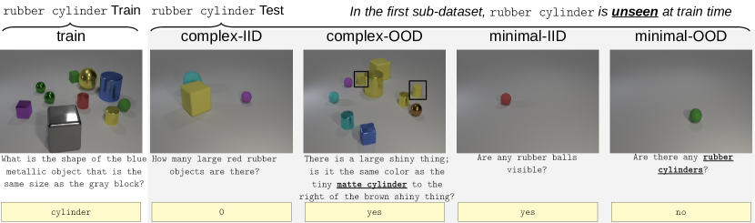
Figure 1: Example image-question pairs for the sub-dataset of CLEVR-HOPE corresponding to rubber cylinder.The test sets are in gray; rubber cylinder is omitted visually and textually in the train split and the IID test splits; rubber cylinder only occurs in the OOD splits; occurrences are emphasized in this figure. The train and complex sets are of comparable visual and textual complexity to CLEVR. The minimal sets consist only of existence questions, checking whether a single object matches a given pair of attribute values.

Our dataset is based on CLEVR Johnson et al. (2017a), a synthetic experimental setting for testing basic visual reasoning skills. CLEVR comprises English questions (such as “What is the color of the cube on the right side of the yellow sphere?") and corresponding 3D-rendered images of colored blocks. Each block has four attribute types (size, color, material, and shape).

We present the CLEVR Held-Out Pair Evaluation (CLEVR-HOPE) dataset for testing the systematicity of VQA models. CLEVR-HOPE is a controlled setting to test whether VQA models generalize to pairs of attribute values that were not seen during either training or fine-tuning. Within CLEVR-HOPE, we refer to an unseen pair of attribute values as a Held-Out Pair (HOP). The dataset is composed of 29 sub-datasets, each for a different HOP (Appx. Tab. 2) . Each HOP has its own train set and 4 test sets. For rubber cylinder, visualized in Fig. 1, these datasets are:

train: 560k image-question pairs in the training/finetuning set. The data distribution is similar to CLEVR, but any images or questions involving rubber cylinder have been removed.

complex-IID test: Test data sampled from the train distribution (i.e., rubber cylinder is filtered out).

complex-OOD test: Test data sampled from the CLEVR distribution filtered to always have (i) at least one object matching rubber cylinder, and (ii) rubber cylinder in the question.

minimal-IID test: Minimal image-question pairs that check whether a model can recognize pairs of attribute values, corresponding to rubber cylinder’s attribute types, that were seen in the train set. E.g., as rubber cylinder is a material-shape combination, the minimal-IID test set checks combinations including rubber spheres, metal cylinders, and metal cubes, but not combinations of different types (e.g., yellow cylinders, or small yellow objects).

minimal-OOD test: Minimal image-question pairs that check recognition of rubber cylinder. Always returning false would yield 75% accuracy.

Appendix A shows complete details. Note that CLEVR-HOPE omits validation sets to prevent hyperparameter tuning for this specific task Teney et al. (2020). Instead, hyperparameters should be chosen using CLEVR.

3 Models & Training

Models: Our analysis focuses on LXMERT Tan and Bansal (2019), a multi-modal transformer-based Vaswani et al. (2017) architecture. We study two LXMERT variants, finetuning each on varying datasets and measuring the systematicity gap. We further run a subset of our experiments on a neurosymbolic model, Tensor-NMN Johnson et al. (2017b), a neural module network Andreas et al. (2016) that decomposes the task into a composition of subtask-specific modules.

Training: For each HOP, we subsample the training set to test the impact the amount of training data has on performance. For 3 random seeds per HOP, we finetune pretrained LXMERT (LXMERT-p) and train LXMERT from scratch (LXMERT-s). We also train Tensor-NMN from scratch, again for three runs, though only for the first 6 HOPs, combinations of {large, cyan, rubber, cylinder}.

For hyperparameter selection, we perform a grid search on the original CLEVR dataset Johnson et al. (2017a). For further details, see Appendix B.

4 Results

4.1 Evidence of Systematic Behaviour

With sufficient training data, over 93% of the tested model-HOP combinations exceed 75% accuracy on the minimal-OOD test set, some reaching 100% (see Appx. Fig. 5). The VQA models have a wide range of accuracies generalizing to different held out pairs. On all models tested, this accuracy varies by around 25% across different HOPs.

Performance on the complex-OOD test set is also generally increasing with the amount of training data, and we see that the OOD accuracies across HOPs are similarly distributed (see Appx. Fig. 7). In all, we can conclude that the models consistently exhibit at least some degree of systematic behaviour. The same trends are observed for Tensor-NMN (see Appx. Figs. 10 and 12).

4.2 Systematicity Gap

Knowing that our models can exhibit systematic behaviour, a natural question to ask is whether there is any trend in the difference between in- and out-of-distribution performance: i.e., as the size of the training set increases (and thus the model’s performance generally improves), does its performance on held-out combinations approach its performance on the combinations already seen at train time? We call this performance difference, between the OOD and IID combinations, the systematicity gap.

For example, if a model has an IID accuracy of 95%, but only 80% for data that requires the model to systematically compose rubber and cylinder into the held out pair rubber cylinder, then the systematicity gap is -15% (i.e., a 15% drop).

Given that the models are somewhat systematic, and that performance in general improves with more training data, one might expect that the systematicity gap would trend to zero. To the contrary, we find that, averaging over all HOPs, the LXMERT systematicity gap plateaus to a drop of 5-6% (see Appx. Fig. 15). On the minimal test sets, the systematicity gap again plateaus, to a drop of 6-8% (see Appx. Fig. 16). The same trends are observed in Tensor-NMN (see Appx. Figs. 17 and 18), though the systematicity gap on minimal examples widens with additional training data.

With that said, the standard deviation of the observed systematicity gap is quite high – in the following section we make the case that the nature of the training data, specifically the attribute diversity seen at train time, is responsible.

4.3 Train-time conceptual diversity impacts systematicity

We define attribute diversity as the number of possible attribute values corresponding to the unseen combination’s attribute types. For example, if the unseen combination is rubber cylinders, that corresponds to the material and shape attribute types. Given there are 2 possible materials and 3 possible shapes in the training set, there are $2\times 3=6$ possible material-shape combinations; thus the attribute diversity is 6.

HOP	Attribute Types	Diversity
Large rubber	Size + Material	4
Rubber cylinder	Material + Shape	6
Large cylinder	Size + Shape	6
Rubber cyan	Material + Color	16
Large cyan	Size + Color	16
Cyan cylinder	Color + Shape	24

Table 1: Diversity of the first six held-out pairs (HOPs). Diversity is the number of possible attribute values corresponding to the HOP’s attribute types.

Tab. 1 lists the attribute diversity of the first six HOPs in CLEVR-HOPE (see Appx. Tab. 2 for all 29 HOPs). Since the CLEVR training distribution is uniform across object attribute values, for a train set of fixed size, as attribute diversity increases, the number of examples per combination decreases.

Fig. 2(a) again illustrates the systematicity gap, but now only averages over HOPs of the same diversity (rather than over all HOPs as in Sec. 4.2). With this, we see that the systematicity gap is stratified by the diversity of the combinations seen at train time. Specifically, as the diversity of the training data increases, the systematicity gap narrows. In fact, the gap is typically near or within a standard deviation of zero for diversities of 16 or above. In comparison, diversities of 6 show a a plateauing systematicity gap stabilizing at 7-14%. As seen in Fig. 2(b), we observe similar results with the systematicity gap of the minimal test sets.

For Tensor-NMN, we also find stratification by diversity for complex examples (see Appx. Fig. 19). The trend on minimal examples is noisier, but converges to the expected ordering (see Appx. Fig. 20).

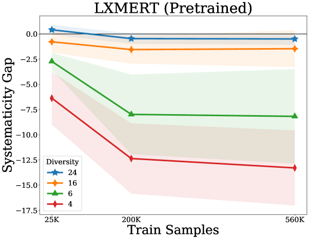
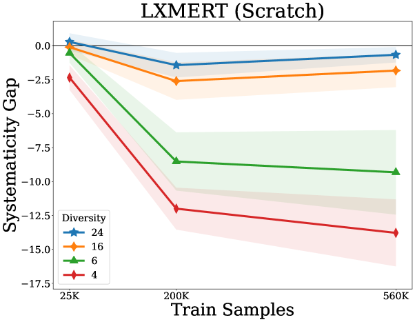
(a) Complex

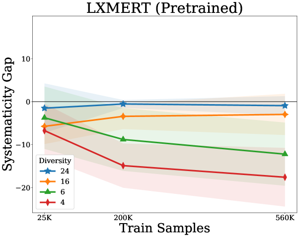
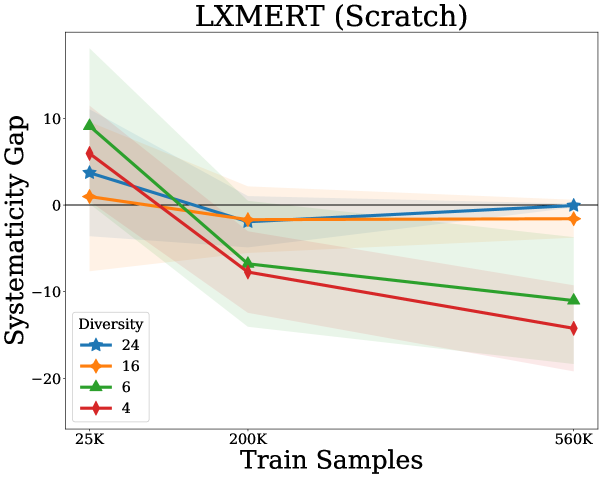
(b) Minimal

Figure 2: Systematicity gap (difference between OOD and IID model accuracy), averaged by held-out pair (HOP) diversity over 29 HOPs, each with 3 runs.

5 Related work

Systematicity has often been investigated through synthetic datasets.  Lake and Baroni (2018) introduced the SCAN benchmark to evaluate the compositionality of sequence-to-sequence models, revealing a lack of systematicity. Followup works Patel et al. (2022); Jiang et al. (2022) have shown that the conceptual diversity of the training set has a significant effect on systematicity — our work extends these findings to the multi-modal domain of VQA.

While compositionality in VQA has been studied, prior work has focused on generalization to new question structures  Bahdanau et al. (2019); Vani et al. (2021); Bogin et al. (2021), or question-answer combinations Agrawal et al. (2017), rather than new attribute combinations. One reason for this gap is that, with natural data, it is hard to control for the model’s exposure to particular attribute combinations. By using a controlled synthetic setting, we can guarantee that generalization behavior is systematic based on the data split.

The closest prior work is the CLEVR-CoGenT dataset:  Johnson et al. (2017a) created a train-test CLEVR split where at train time cubes and cylinders are restricted to limited color palettes, that are reversed at test time. They observed that model performance declined on held-out attribute combinations. But, unlike CLEVR-HOPE, CLEVR-CoGenT does not change the question distribution at train time — held-out combinations can leak by appearing in text at train time. Furthermore, CLEVR-CoGenT has only a single train set with held-out color-shape combinations — whereas CLEVR-HOPE expands the set of held-out combinations to 29 train sets, covering all possible pairs of attribute types. CLEVR-HOPE also independently assesses each HOP, including in a minimal setting. In combination, these improvements allow us to study the impact of train-time diversity.

Beyond CLEVR-CoGenT, our results align with concurrent work on the effects of training diversity in VQA: Rahimi et al. (2023) modify CLEVR to study the related question of productivity. Specifically, generalization to questions with more reasoning steps, and generalization to new question combinations (e.g., answering counting questions about shape, when all train-time counting questions are about color or size). They conclude that increasing the diversity of question combinations increases productivity. Unlike our work, they do not use a transformer architecture, instead studying MAC Hudson and Manning (2018), FiLM Perez et al. (2018), and Vector-NMN Bahdanau et al. (2019). Additionally, as they study a fundamentally different question, their dataset only alters the question distribution — their image distribution is unchanged between train and test time.

Given that both systematicity and productivity fall under the larger umbrella of compositional generalization Hupkes et al. (2020), and given the wide variety of architectures collectively studied between both our and existing work, the combined weight of the evidence suggests a close relationship between train-time diversity and compositional generalization as a broad phenomenon.

6 Conclusions

Using CLEVR-HOPE, we demonstrate that LXMERT and Tensor-NMN exhibit some degree of systematic generalization to held-out object attribute pairs. Furthermore, we illustrate that the systematicity gap (the difference between in- and out-of-distribution performance) does not improve with more data, but does with more attribute diverse data— i.e., the number of attribute pairs of the same type seen at train time.

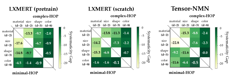
Figure 3: Systematicity gap on the complex splits (top corner) and minimal splits (bottom corner) for all models trained on 560k training examples. The systematicity gap is averaged according to the attribute types of the HOPs, all 29 HOPs for LXMERT, HOPs 0-5 for Tensor-NMN — attributes are sorted by increasing diversity on the axes (e.g., shape has 2 possible values, color has 8 possible values). As expected, we see a worse systematicity gap (i.e. lighter colors) in the top left (low-diversity combinations), and better systematicity gap (i.e., darker colors) in the bottom right (high-diversity combinations).

Limitations

First and foremost, while the synthetic nature of CLEVR-HOPE allows for a more controlled study of models, it raises the question whether the observed results will hold in more complex and diverse real-world settings. Furthermore, as we did not modify the CLEVR attribute values, HOP diversity is intrinsically tied to attribute type. e.g., the most diverse pairs are always shape-color combinations, and the least diverse pairs are always material-size combinations. Thus, it is possible that we are actually measuring the effects of attribute type on generalization, rather than diversity.

However, in visualizing the systematicity gap by attribute-types in the pair on both LXMERT and Tensor-NMN (see Fig. 3), we can see that while the systematicity gap tends to be larger for material than size (with these attribute types both having two possible values, i.e. the same diversity), it still holds that the systematicity gaps are still sorted by the diversity of the attribute pairs. In addition, with respect to raw accuracy, we find that LXMERT tends to struggle when Shape-Material pairs (diversity 6) are held out — more so than with the lower diversity Material-Size pairs (diversity 4) (see Appx. Fig. 9). Yet despite this, the systematicity gaps remain sorted as expected — i.e., worse on the lower diversity Material-Size pairs (see Fig. 3). Finally, our results are supported by prior work in other domains Patel et al. (2022); despite the number of examples per combination decreasing with increasing diversity, the systematicity gap still tends to improve.

The second major limitation arises from the choice of models. LXMERT uses a pretrained F-RCNN Ren et al. (2015) for object detection, which we do not alter. As the F-RCNN is pretrained, it may already possess implicit knowledge of the attributes (e.g., shape), and may contribute systematic structure to LXMERT. Any such visual knowledge or biases are therefore given to both LXMERT-p and LXMERT-s. In contrast, note that the language component of LXMERT-s is randomly initialized — whereas Tan and Bansal (2019) initialized their language transformer with BERT Devlin et al. (2019) when pretraining from scratch.

Finally, due to time and resource limitations we were unable to evaluate Tensor-NMN on HOP-6 through 28.

Appendix A CLEVR-HOPE: Additional details

The full list of held-out pairs (HOPs) can be found in Table 2. The HOPs were selected by choosing two attribute values from each of large cyan rubber cylinder, small brown rubber sphere, small red metal cylinder, large gray metal cube, and small purple rubber sphere.

Note that there are only 4 possible material-size combinations, as there are only 2 sizes and 2 materials. We include all 4 of these, as well as 5 HOPs for every other pair of attribute types.

Before selecting the 5 4-tuples from which we created the HOPs in CLEVR-HOPE, we first created a small set of minimal test questions for testing how well a given model comprehends a given attribute in isolation — CLEVR-PRELIM. For example, for the color cyan we had two types of tests. First, tests similar to the minimal-OOD test tests (i.e., a single object and rephrasings of “Are any cyan objects visible?”). Second, counting tests — all questions were rephrases of “What number of cyan objects are there?”, and images had varying numbers of cyan objects. Specifically, we fixed the position of 5 objects, and created 6 images, each with a different number of objects matching the attribute — i.e., 0, 1, 2, 3, 4, or 5 cyan objects.

Note that, unlike CLEVR-HOPE which studies pairs of attributes values, CLEVR-PRELIM evaluates only attribute values in isolation.

Using CLEVR-PRELIM, we performed a zero-shot evaluation of Tan and Bansal (2019)’s VQA2.0 Goyal et al. (2017) fine-tuned LXMERT checkpoint. From this preliminary study we found that zero-shot model performance was generally poor (e.g., over all attribute values of all types, the highest count performance was 49.1%). Given our interest in studying the impact of the amount of training data, we created our first 4-tuple by individually selecting each attribute value; specifically choosing the attribute value that zero-shot LXMERT had the lowest performance on — this created the 4-tuple Large cyan rubber cylinder. The remaining four tuples were selected uniformly at random. Ultimately, as we did not see any significant difference between a small sample of 6 HOPs (those created from attribute pairs in large cyan rubber cylinder) and a larger sample of 23 HOPs (those created from random 4-tuples), we present results aggregated over all 29 HOPs.

Note that as two 4-tuples were rubber spheres and small spheres, we added the HOPs rubber cube and small cube so that we would maintain five material-shape and five size-shape pairs.

HOP	Attribute Types	Diversity
Large rubber	Size + Material	4
Small rubber	Size + Material	4
Large metal	Size + Material	4
Small metal	Size + Material	4
Rubber cylinder	Material + Shape	6
Metal cylinder	Material + Shape	6
Rubber cube	Material + Shape	6
Metal cube	Material + Shape	6
Rubber sphere	Material + Shape	6
Large cylinder	Size + Shape	6
Small cylinder	Size + Shape	6
Small cube	Size + Shape	6
Large cube	Size + Shape	6
Small sphere	Size + Shape	6
Rubber cyan	Material + Color	16
Rubber brown	Material + Color	16
Rubber purple	Material + Color	16
Metal red	Material + Color	16
Metal gray	Material + Color	16
Large cyan	Size + Color	16
Small brown	Size + Color	16
Small purple	Size + Color	16
Small red	Size + Color	16
Large gray	Size + Color	16
Cyan cylinder	Color + Shape	24
Brown sphere	Color + Shape	24
Red cylinder	Color + Shape	24
Gray cube	Color + Shape	24
Purple sphere	Color + Shape	24

Table 2: Train set diversity of each held-out pair (i.e., HOP) of object attribute values. Diversity is the number of possible pairs of attribute values, corresponding to the HOPs attribute types.

For each HOP in CLEVR-HOPE, the approximate size of the corresponding splits is outlined below:

• train set: 62k images, and 560k image-question pairs

• complex-IID test set: 13k images, 120k image-question pairs

• complex-OOD test set: 15k images, 15k image-question pairs

• minimal-IID test set: 2576-3200 images, 8640-11970 image-question pairs (depending on HOP)

• minimal-OOD test set: 448-3840 images, 448-3840 image-question pairs (depending on HOP)

To reduce the resources required to generate the dataset, images are reused throughout the dataset. Specifically, the images are reused across the train sets for the HOPs, and reused from the original CLEVR training set.

Similarly, each of the test sets reuse images across HOPs. Note that while the complex-IID test and complex-OOD test sets do not reuse eachother’s images, the minimal-IID test and minimal-OOD test sets do for images that do not involve the HOP under consideration.

To ensure that CLEVR can be fairly used for hyperparameter tuning, and to prevent any data leakage, no CLEVR validation or test images are reused in CLEVR-HOPE.

A.1 CLEVR-HOPE: minimal-OOD test set and minimal-IID test set

All images in the minimal-OOD test and minimal-IID test sets contain only a single object. All questions ask whether there are any objects matching the attribute value pair. E.g., for the HOP rubber cyan, some question variants include “Are there any cyan matte things?” and “Are any cyan matte things visible?”.

These splits are designed to test the model in a systematic manner: each image matching the HOP has 3 corresponding images that do not match the HOP. These 4 images share identical question phrasing. The non-matching images maintain the object position, lighting, and the attribute values that are irrelevant to the HOP, but change the first attribute value in the HOP, the second attribute value in the HOP, or both attribute values in the HOP, respectively. See Fig. 4 for an example.

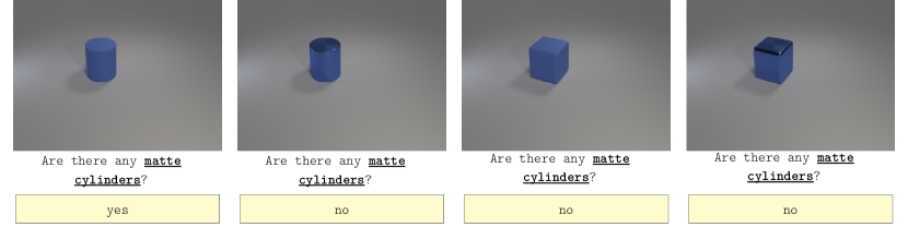
Figure 4: Four example image-question pairs for the minimal-OOD test split of the sub-dataset of CLEVR-HOPE corresponding to the first held-out attribute pair — i.e., rubber cylinder. Note how the first image matches rubber cylinder (material=rubber, and shape=cylinder), and the next three image have one attribute value (material=metal), the other attribute value (shape=cube), or both (material=metal, and shape=cube) attribute values not matching rubber cylinder. This pattern repeats throughout the dataset, with the choice of distractor values, object position, lightning, question-phrasing and the value of the attribute-types not in HOP, all chosen randomly, but fixed within each set of 4 images.

Note that the question template is taken directly from the original CLEVR dataset generation code. The main change is the aforementioned systematic design, and that the images used contain only a single object, whereas the original CLEVR requires at least 3 objects in any scene.

The minimal-IID test split is created in the same way, but testing all other attribute-value pairs of the same type as the HOP. Note that the distractor attribute values in the negative examples were selected uniformly at random. Since this may create the held-out pair (and indeed, must do so for one of the four size-material images), after the initial creation of the minimal-IID test split, we filter it to remove any image-question pairs where the object in the image matches the HOP.

Appendix B Training details

All subsets of the train sets (i.e., of size 25k, 200k, and 560k) are created by taking the first however many indices. This corresponds to a random subset of images for 25k, which is consecutively randomly expanded. This is so because the image-question pairs are unsorted, apart from all questions for any given image having contiguous indices. Note that we fix the number of gradient updates across subset sizes, i.e., smaller subsets are trained for more epochs so that the total number of gradient updates is the same.

Hyperparameter	LXMERT-p	LXMERT-s
Learning Rate	5e-5	1e-5
Gradient Updates	218,750	481,000
Batch size	32	32

Table 3: Key hyperparameter values used for LXMERT

For LXMERT, the maximum sequence length is increased to 49 so that CLEVR-HOPE questions are not truncated.

For LXMERT-p, we follow Tan and Bansal (2019)’s procedure for finetuning their pretrained LXMERT checkpoint on a VQA dataset. As part of their procedure, the pretrained F-RCNN Ren et al. (2015) object detector is not altered in any way.

LXMERT-p hyperparameters were modified from the hyperparameters used by Tan and Bansal (2019) for finetuning LXMERT for VQA. Specifically, Tan and Bansal (2019) finetuned LXMERT for the VQA tasks of VQAv2 Goyal et al. (2017), NLVR2 Suhr et al. (2019), and GQA Hudson and Manning (2019) with a batch size of 32, 4 epochs, and a learning rate of either 1e-5 or 5e-5. We ultimately used a learning rate of 5e-5, and increased the epochs to 10 as we found it yielded better performance.

For LXMERT-s we randomly initialize all LXMERT weights (this excludes the pretrained F-RCNN object detector), and apply the LXMERT finetuning procedure (albeit with different hyperparamters) to train this randomly initialized model.

LXMERT-s hyperparameter tuning was performed via grid search over learning rate (1e-4, 5e-5, 1e-5) and training steps (218750, 481000, 700000). Note that we ultimately used 481k gradient update steps, as its validation accuracy (95.47%) was extremely close to 700k (96.99%), with nearly half the training time.

The LXMERT hyperparameters used are summarized in Tab. 3.

Tensor-NMN is trained from scratch following the process used by Bahdanau et al. (2019). Tensor-NMN is trained in a 3 stage process — initially the program generator and execution engine are trained in a supervised manner, following which they are trained together using REINFORCE. The default hyperparameters for CLEVR from Bahdanau et al. (2019) are used.

Appendix C LXMERT Detailed Results

LXMERT performance on minimal-OOD test can be found in Fig. 5. Performance on minimal-IID test can be found in Fig. 6. All plots mark 75% — this baseline performance is achieved on the minimal-OOD test split by always predicting false (i.e., the most common class). Always predicting false on minimal-IID test yield a baseline performance between 66% and 75%, depending on the HOP.

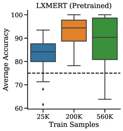
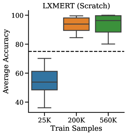
Figure 5: Box plot of minimal-OOD test set performance on all 29 HOPs. The average performance for each HOP is produced by averaging over 3 trials. The variation captured by this boxplot is from the difference in average performance between HOPs, rather than from the variation within the 3 trials.

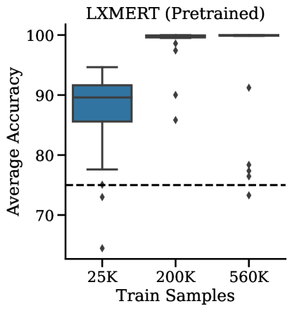
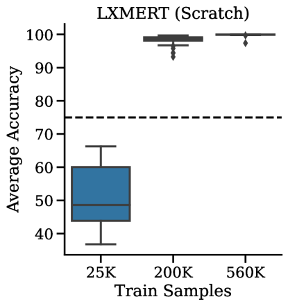
Figure 6: Box plot of minimal-IID test set performance on all 29 HOPs. The average performance for each HOP is produced by averaging over 3 trials. The variation captured by this boxplot is from the difference in average performance between HOPs, rather than from the variation within the 3 trials.

LXMERT performance on complex-OOD test can be found in Fig. 7. Performance on complex-IID test can be found in Fig. 8.

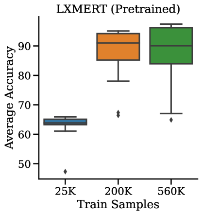
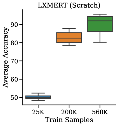
Figure 7: Box plot of complex-OOD test set performance on all 29 HOPs. The average performance for each HOP is produced by averaging over 3 trials. The variation captured by this boxplot is from the difference in average performance between HOPs, rather than from the variation within the 3 trials.

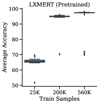
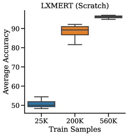
Figure 8: Box plot of complex-IID test set performance on all 29 HOPs. The average performance for each HOP is produced by averaging over 3 trials. The variation captured by this boxplot is from the difference in average performance between HOPs, rather than from the variation within the 3 trials.

For LXMERT trained on the largest train sets (560k), we plot the complex and minimal model accuracies, averaged by the attribute types of the HOPs, in Fig. 9.

Figure 9: Model accuracies for HOP-0 through 28. Note that the LXMERT models often struggle on both IID and OOD questions when Material-Shape combinations are held out at train time.

Appendix D Tensor-NMN Detailed Results

As Tensor-NMN was only evaluated on the first 6 HOPs, we include the subset of LXMERT models trained on the same HOPs for comparison.

Model performance on minimal-OOD test can be found in Fig. 10. Performance on minimal-IID test can be found in Fig. 11. All plots mark 75% — this baseline performance is achieved on the minimal-OOD test split by always predicting false (i.e., the most common class). Always predicting false on minimal-IID test yield a baseline performance between 66% and 75%, depending on the HOP.

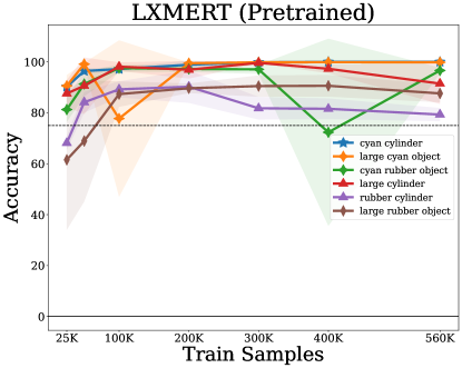
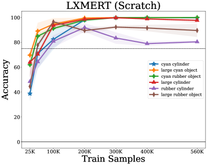
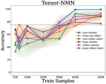
Figure 10: Average minimal-OOD test set Tensor-NMN performance for the first 6 HOPs over 3 trials. For comparison, we also plot the average LXMERT model performances (i.e., Fig. 5), but restricted to only the first 6 HOPs. An area corresponding to 1 standard deviation is shaded.

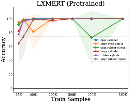
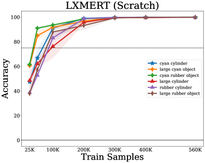
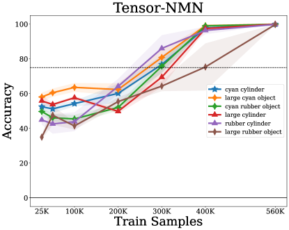
Figure 11: Average minimal-IID test set Tensor-NMN performance for the first 6 HOPs over 3 trials. For comparison, we also plot the average LXMERT model performances (i.e., Fig. 6), but restricted to only the first 6 HOPs. An area corresponding to 1 standard deviation is shaded.

Model performance on complex-OOD test can be found in Fig. 12. Performance on complex-IID test can be found in Fig. 13.

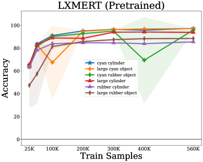
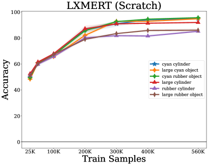
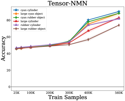
Figure 12: Average complex-OOD test set Tensor-NMN performance for the first 6 HOPs over 3 trials. For comparison, we also plot the average LXMERT model performances (i.e., Fig. 7), but restricted to only the first 6 HOPs. An area corresponding to 1 standard deviation is shaded.

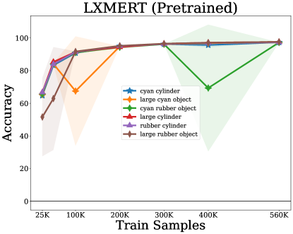
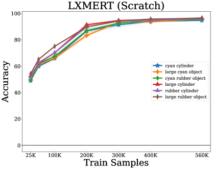
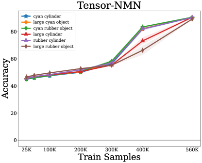
Figure 13: Average complex-IID test set Tensor-NMN performance for the first 6 HOPs over 3 trials. For comparison, we also plot the average LXMERT model performances (i.e., Fig. 8), but restricted to only the first 6 HOPs. An area corresponding to 1 standard deviation is shaded.

For Tensor-NMN trained on the largest train sets (560k), we plot the complex and minimal model accuracies, averaged by the attribute types of the HOPs. The results are visualized in Fig. 14. Again, we include the corresponding subset of LXMERT models for comparison.

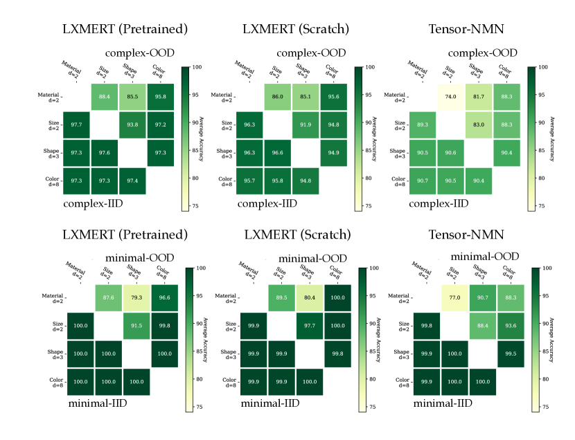
Figure 14: Model accuracies for only the first 6 HOPs. Note that while the LXMERT models struggle with Material-Shape combinations on OOD questions, Tensor-NMN does not.

Appendix E Systematicity Gap

As outlined in Section 4.2, we find that, on all models, averaged over HOPs, the gap between performance on complex questions involving IID vs. OOD attribute combinations does not trend to zero. Instead, it plateaus (see Figures 15 and 17). In comparison, the performance gap on minimal questions plateaus or decreases gently (see Figures 16 and 18).

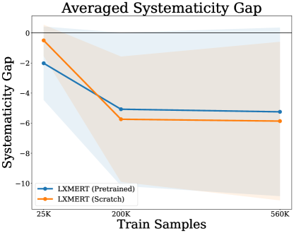
Figure 15: Average systematicity gap on complex examples (i.e., complex-OOD test accuracy minus complex-IID test accuracy) with 1 standard deviation; averaged over 3 runs on each of the 29 HOPs. Note that the systematicity gap plateaus, suggesting that the performance drop when generalizing to unseen combinations does not improve with additional training data.

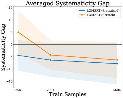
Figure 16: Average systematicity gap on minimal examples (i.e., minimal-OOD test accuracy minus minimal-IID test accuracy) with 1 standard deviation; averaged over 3 runs on each of the 29 HOPs.

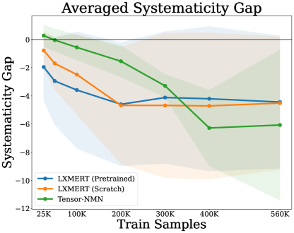
Figure 17: Average systematicity gap on complex examples (i.e., complex-OOD test accuracy minus complex-IID test accuracy) with 1 standard deviation; averaged over 3 runs on only the first 6 HOPs. Note that the systematicity gap plateaus, suggesting that the performance drop when generalizing to unseen combinations does not improve with additional training data.

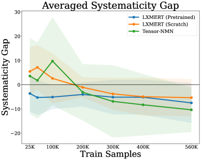
Figure 18: Average systematicity gap on minimal examples (i.e., minimal-OOD test accuracy minus minimal-IID test accuracy) with 1 standard deviation; averaged over 3 runs on only the first 6 HOPs.

E.1 Detailed Tensor-NMN Systematicity Gap

Averaging the systematicity gap in Tensor-NMN by diversity, we again find stratification by diversity for complex examples (see Fig. 19). The trend on minimal examples is noisier, but ultimately converges to the expected ordering (see Fig. 20). Note that, as is to be expected, when limited to the first six HOPs the LXMERT trend is also noisier. It is therefore reasonable to expect the Tensor-NMN trend would be cleaner with additional HOPs.

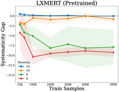
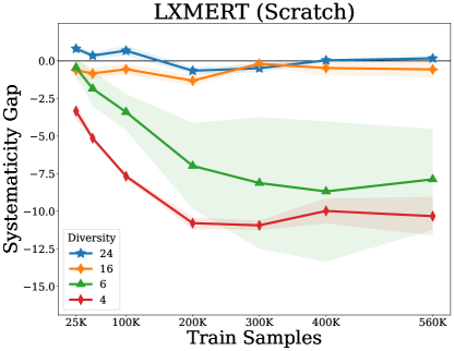
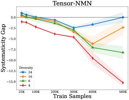
Figure 19: Systematicity gap (i.e. difference between OOD and IID model performance) for complex examples, averaged by HOP diversity over for the first 6 held-out attribute pairs only, each with 3 runs.

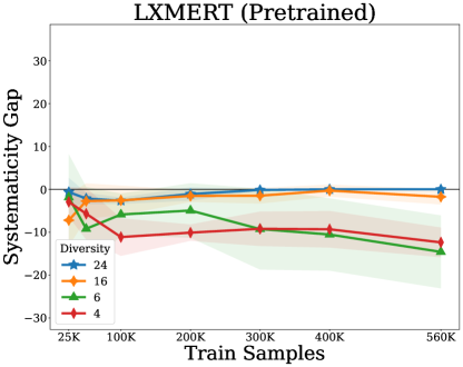
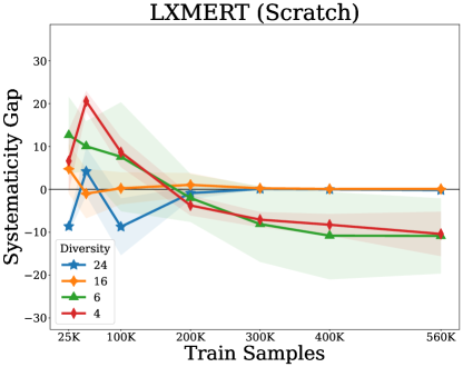
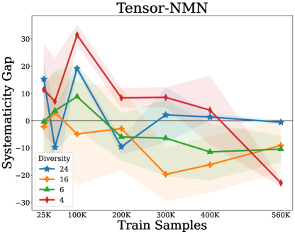
Figure 20: Systematicity gap (i.e. difference between OOD and IID model performance) for minimal examples, averaged by HOP diversity over for the first 6 held-out attribute pairs only, each with 3 runs.

References

- Agrawal et al. (2017) Aishwarya Agrawal, Aniruddha Kembhavi, Dhruv Batra, and Devi Parikh. 2017. C-VQA: A compositional split of the visual question answering (VQA) v1.0 dataset. CoRR, abs/1704.08243.
- Andreas et al. (2016) Jacob Andreas, Marcus Rohrbach, Trevor Darrell, and Dan Klein. 2016. Neural module networks. In Proceedings of the IEEE conference on computer vision and pattern recognition, pages 39–48.
- Bahdanau et al. (2019) Dzmitry Bahdanau, Harm de Vries, Timothy J O’Donnell, Shikhar Murty, Philippe Beaudoin, Yoshua Bengio, and Aaron Courville. 2019. Closure: Assessing systematic generalization of clevr models. arXiv preprint arXiv:1912.05783.
- Bogin et al. (2021) Ben Bogin, Shivanshu Gupta, Matt Gardner, and Jonathan Berant. 2021. COVR: A test-bed for visually grounded compositional generalization with real images. In Proceedings of the 2021 Conference on Empirical Methods in Natural Language Processing, pages 9824–9846, Online and Punta Cana, Dominican Republic. Association for Computational Linguistics.
- Csordás et al. (2021) Róbert Csordás, Kazuki Irie, and Jürgen Schmidhuber. 2021. Learning adaptive control flow in transformers for improved systematic generalization. In Advances in Programming Languages and Neurosymbolic Systems Workshop.
- Csordás et al. (2022a) Róbert Csordás, Kazuki Irie, and Jürgen Schmidhuber. 2022a. The devil is in the detail: Simple tricks improve systematic generalization of transformers.
- Csordás et al. (2022b) Róbert Csordás, Kazuki Irie, and Jürgen Schmidhuber. 2022b. The neural data router: Adaptive control flow in transformers improves systematic generalization.
- Devlin et al. (2019) Jacob Devlin, Ming-Wei Chang, Kenton Lee, and Kristina Toutanova. 2019. BERT: Pre-training of deep bidirectional transformers for language understanding. In Proceedings of the 2019 Conference of the North American Chapter of the Association for Computational Linguistics: Human Language Technologies, Volume 1 (Long and Short Papers), pages 4171–4186, Minneapolis, Minnesota. Association for Computational Linguistics.
- Fodor and Pylyshyn (1988) Jerry A Fodor and Zenon W Pylyshyn. 1988. Connectionism and cognitive architecture: A critical analysis. Cognition, 28(1-2):3–71.
- Goyal et al. (2017) Yash Goyal, Tejas Khot, Douglas Summers-Stay, Dhruv Batra, and Devi Parikh. 2017. Making the V in VQA matter: Elevating the role of image understanding in Visual Question Answering. In Conference on Computer Vision and Pattern Recognition (CVPR).
- Hudson and Manning (2018) Drew A. Hudson and Christopher D. Manning. 2018. Compositional attention networks for machine reasoning. In 6th International Conference on Learning Representations, ICLR 2018, Vancouver, BC, Canada, April 30 - May 3, 2018, Conference Track Proceedings. OpenReview.net.
- Hudson and Manning (2019) Drew A Hudson and Christopher D Manning. 2019. Gqa: A new dataset for real-world visual reasoning and compositional question answering. In Proceedings of the IEEE/CVF conference on computer vision and pattern recognition, pages 6700–6709.
- Hupkes et al. (2020) Dieuwke Hupkes, Verna Dankers, Mathijs Mul, and Elia Bruni. 2020. Compositionality decomposed: How do neural networks generalise? J. Artif. Intell. Res., 67:757–795.
- Jiang et al. (2022) Yichen Jiang, Xiang Zhou, and Mohit Bansal. 2022. Mutual exclusivity training and primitive augmentation to induce compositionality. In Proceedings of the 2022 Conference on Empirical Methods in Natural Language Processing, pages 11778–11793, Abu Dhabi, United Arab Emirates. Association for Computational Linguistics.
- Johnson et al. (2017a) Justin Johnson, Bharath Hariharan, Laurens van der Maaten, Li Fei-Fei, C Lawrence Zitnick, and Ross Girshick. 2017a. Clevr: A diagnostic dataset for compositional language and elementary visual reasoning. In CVPR.
- Johnson et al. (2017b) Justin Johnson, Bharath Hariharan, Laurens van der Maaten, Judy Hoffman, Li Fei-Fei, C. Lawrence Zitnick, and Ross B. Girshick. 2017b. Inferring and executing programs for visual reasoning. In IEEE International Conference on Computer Vision, ICCV 2017, Venice, Italy, October 22-29, 2017, pages 3008–3017. IEEE Computer Society.
- Lake and Baroni (2018) Brenden Lake and Marco Baroni. 2018. Generalization without systematicity: On the compositional skills of sequence-to-sequence recurrent networks. In International conference on machine learning, pages 2873–2882. PMLR.
- Patel et al. (2022) Arkil Patel, Satwik Bhattamishra, Phil Blunsom, and Navin Goyal. 2022. Revisiting the compositional generalization abilities of neural sequence models. In Proceedings of the 60th Annual Meeting of the Association for Computational Linguistics (Volume 2: Short Papers), pages 424–434, Dublin, Ireland. Association for Computational Linguistics.
- Perez et al. (2018) Ethan Perez, Florian Strub, Harm de Vries, Vincent Dumoulin, and Aaron C. Courville. 2018. Film: Visual reasoning with a general conditioning layer. In Proceedings of the Thirty-Second AAAI Conference on Artificial Intelligence, (AAAI-18), the 30th innovative Applications of Artificial Intelligence (IAAI-18), and the 8th AAAI Symposium on Educational Advances in Artificial Intelligence (EAAI-18), New Orleans, Louisiana, USA, February 2-7, 2018, pages 3942–3951. AAAI Press.
- Press et al. (2022) Ofir Press, Muru Zhang, Sewon Min, Ludwig Schmidt, Noah A Smith, and Mike Lewis. 2022. Measuring and narrowing the compositionality gap in language models. arXiv preprint arXiv:2210.03350.
- Rahimi et al. (2023) Amir Rahimi, Vanessa D’Amario, Moyuru Yamada, Kentaro Takemoto, Tomotake Sasaki, and Xavier Boix. 2023. D3: Data diversity design for systematic generalization in visual question answering. arXiv preprint arXiv:2309.08798.
- Ren et al. (2015) Shaoqing Ren, Kaiming He, Ross Girshick, and Jian Sun. 2015. Faster r-cnn: Towards real-time object detection with region proposal networks. In Advances in Neural Information Processing Systems, volume 28. Curran Associates, Inc.
- Suhr et al. (2019) Alane Suhr, Stephanie Zhou, Ally Zhang, Iris Zhang, Huajun Bai, and Yoav Artzi. 2019. A corpus for reasoning about natural language grounded in photographs. In Proceedings of the 57th Annual Meeting of the Association for Computational Linguistics, pages 6418–6428, Florence, Italy. Association for Computational Linguistics.
- Tan and Bansal (2019) Hao Tan and Mohit Bansal. 2019. Lxmert: Learning cross-modality encoder representations from transformers. arXiv preprint arXiv:1908.07490.
- Teney et al. (2020) Damien Teney, Ehsan Abbasnejad, Kushal Kafle, Robik Shrestha, Christopher Kanan, and Anton Van Den Hengel. 2020. On the value of out-of-distribution testing: An example of goodhart’s law. Advances in neural information processing systems, 33:407–417.
- Vani et al. (2021) Ankit Vani, Max Schwarzer, Yuchen Lu, Eeshan Dhekane, and Aaron Courville. 2021. Iterated learning for emergent systematicity in vqa. In International Conference on Learning Representations.
- Vaswani et al. (2017) Ashish Vaswani, Noam Shazeer, Niki Parmar, Jakob Uszkoreit, Llion Jones, Aidan N Gomez, Łukasz Kaiser, and Illia Polosukhin. 2017. Attention is all you need. Advances in neural information processing systems, 30.