Fast Parallel Tensor Times Same Vector for Hypergraphs

Abstract

Hypergraphs are a popular paradigm to represent complex real-world networks exhibiting multi-way relationships of varying sizes. Mining centrality in hypergraphs via symmetric adjacency tensors has only recently become computationally feasible for large and complex datasets. To enable scalable computation of these and related hypergraph analytics, here we focus on the Sparse Symmetric Tensor Times Same Vector (S³TTVc) operation. We introduce the Compound Compressed Sparse Symmetric (CCSS) format, an extension of the compact CSS format for hypergraphs of varying hyperedge sizes and present a shared-memory parallel algorithm to compute S³TTVc. We experimentally show S³TTVc computation using the CCSS format achieves better performance than the naive baseline, and is subsequently more performant for hypergraph $H$-eigenvector centrality.

I Introduction

Hypergraphs are generalizations of graphs that represent multi-entity relationships in a broad range of domains, such as cybersecurity [1, 2], biological systems [3], social networks [4], and telecommunications[5]. While graph edges connect exactly two nodes, hyperedges may connect any number of nodes. Most real-world hypergraphs are non-uniform, meaning they have differently sized hyperedges, which poses challenges for their compact representation and analysis.

For uniform hypergraphs, symmetric tensors are popularly used to represent the higher-order adjacency information [6, 7]. Several strategies have been explored to extend the tensor representation approach to non-uniform hypergraphs, including adding dummy nodes [8, 9], considering the set of symmetric adjacency tensors, with each tensor arising from the component uniform hypergraph of a particular hyperedge size [10, 11], and combinatorially inflating the lower–cardinality hyperedges until all hyperedges are equisized [12]. Following Aksoy, Amburg, and Young [13], we call these inflated hyperedges blowups and focus on the adjacency tensor as defined by Banerjee et al. [12], which we call the blowup tensor.

S³TTVc is a key operation on symmetric tensors, and is the computational bottleneck in fundamental algorithms such as the shifted-power method for computing tensor eigenpairs and symmetric CP-decomposition [14, 15, 16]. These algorithms, in turn, are utilized to perform a variety of hypergraph analyses. For instance, eigenpairs of the adjacency tensor of uniform hypergraphs are used to define $H$-eigenvector centrality (HEC) [17], a nonlinear hypergraph centrality measure which was further extended to non-uniform hypergraphs using the blowup tensor representation [13]. Thus, developing performant algorithms for S³TTVc on the blowup tensor enables efficient computation of hypergraph centrality.

However, working with the blowup tensor requires we overcome several computational challenges. First, since enumerating all its nonzeros is prohibitively costly, following Aksoy, Amburg, and Young, we will adapt the “generating function approach” [13], to perform the computation indirectly. Second, we introduce a new, compressed format for tensors that is tailored to reduce the memory footprint of storing nonuniform hypergraphs, called Compound Compressed Sparse Symmetric (CCSS). This extends past work on the CSS format for uniform hypergraphs[18, 19] and, as explained further in Section IV, achieves S³TTVc performance gains via memoization of intermediate results.

Our main contributions are summarized as follows:

• We introduce the Compound Compressed Sparse Symmetric (CCSS), an extension of the CSS format for non-uniform hypergraphs, and demonstrate up to $26.4\times$ compression compared to coordinate storage format for real-world hypergraphs.

• We implement an efficient multi-core parallel S³TTVc algorithm, called CCSS-MEMO which adapts the generating function approach to the CCSS format, and identifies opportunities for memoization of intermediate results.

• We present two baseline approaches which use the CCSS without memoization and adopt two state-of-the-art approaches to highlight the performance of CCSS-MEMO. We realize up to $53.98\times$ speedup compared to CCSS-DIRECT, and up to $12.45\times$ speedup compared to CCSS-FFT.

• We apply our algorithm to the calculation of $H$-eigenvector centrality for hypergraphs, obtaining speedups of many orders of magnitude over state-of-the-art approaches.

II Preliminaries

Following Kolda and Bader [20], we denote vectors using bold lowercase letter (e.g., $\bm{\mathbf{{a}}}$, $\bm{\mathbf{{b}}}$), and tensors using bold calligraphic letters (e.g., $\bm{\mathscr{{X}}}$). For a tensor $\bm{\mathscr{{X}}}$ and a vector ${\bm{\mathbf{{b}}}}$ we will also denote by $\bm{\mathscr{{X}}}\times_{j}{\bm{\mathbf{{b}}}}$ the product of $\bm{\mathscr{{X}}}$ and ${\bm{\mathbf{{b}}}}$ along the $j^{\textrm{th}}$-mode of $\bm{\mathscr{{X}}}$ resulting in a order $(N-1)$ tensor. Using this notation, we can define Tensor-Time-Same-Vector in all modes but 1 (TTSV1)

$$\bm{\mathbf{{s}}}=\bm{\mathscr{{X}}}\bm{\mathbf{{b}}}^{N-1}=\bm{\mathscr{{X}}}=\bm{\mathscr{{X}}}\times_{2}\bm{\mathbf{{b}}}\times_{3}\bm{\mathbf{{b}}}\ldots\times_{N}\bm{\mathbf{{b}}}$$ (1)

which plays an important role in calculating generalized eigenvalues and eigenvectors associated with $\bm{\mathscr{{X}}}.$ Alternatively, by expanding along indicies this may be rewritten as

$$s_{i_{1}}=\left[\bm{\mathscr{{X}}}{\bm{\mathbf{{b}}}}^{N-1}\right]_{i_{1}}=\sum_{i_{2}=1}^{n}\cdots\sum_{i_{N}=1}^{n}\bm{\mathscr{{X}}}_{i_{1},\dots,i_{N}}\prod_{k=2}^{N}{\bm{\mathbf{{b}}}}_{i_{k}}.$$ (2)

Formally, a hypergraph is a pair $H=(V,E)$, where $V$ is the set of vertices, and $H$ is the set of hyperedges on those vertices; that is, $E$ is some subset of the power set of $V$. We say $H$ is uniform if all hyperedges have the same size; otherwise, it is nonuniform. The rank of $H$ is the size of the largest hyperedge.

An order-$N$ symmetric tensor $\bm{\mathscr{{X}}}$ has $N$ modes or dimensions, with the special property that the values, $\bm{\mathscr{{X}}}_{(i_{1},i_{2},\ldots i_{N})}$ remains unchanged under any permutation of its indices. Symmetric tensors arise naturally in many context including the representation of hypergraphs. For example, if $H$ is an $N$-uniform hypergraph on $n$ vertices, there is natural symmetric representation as an order-$N$ tensor $\bm{\mathscr{{X}}}\in\mathbb{R}^{n\times n\times\cdots\times n}$. That is, for every hyperedge $e=\{v_{i_{1}},v_{i_{2}},\ldots,v_{i_{N}}\}\in E$ with weight $w(e)$, $\bm{\mathscr{{X}}}_{\sigma(\bm{\mathbf{{i}}})}=\frac{w(e)}{N!}$, where $\sigma(\bm{\mathbf{{i}}})$ denotes any of the $N!$ permutations of the index tuple $\bm{\mathbf{{i}}}=(i_{1},\ldots,i_{N})$. In order to extend this representation to non-uniform hypergraphs, we follow the approach of Banerjee et al. [12] and define for a rank-$N$ edge-weighted hypergraph $H=(V,E,w)$ the order-$N$ blowup tensor, $\bm{\mathscr{{B}}}$, associated with $H$. To this end, for each edge $e\in H$ define the set of ordered blowups of $e$ as

$$\beta(e)=\left\{i_{1},i_{2},\ldots i_{N}:\text{for each }v\in e,\exists j\ni i_{j}=v\right\}.$$

Then for each ${\bm{\mathbf{{i}}}}\in\beta(e)$, $\bm{\mathscr{{B}}}_{{\bm{\mathbf{{i}}}}}$ has value $\frac{w(e)}{|\beta(e)|}$. As we be working primarily with the blowup tensor, it will be convenient to define $\mathcal{E}(\bm{\mathscr{{B}}})$ as the collection of edges which generated the blowup tensor $\bm{\mathscr{{B}}}$. In this paper, we take $w(e)=\lvert e\rvert$ to ensure that $\bm{\mathscr{{B}}}\bm{\mathbf{{1}}}^{N-1}=\bm{\mathbf{{d}}},$ the vector of node degrees. It is worth noting that for uniform hypergraphs, $\bm{\mathscr{{B}}}$ is precisely the uniform adjacency tensor of the hypergraph discussed above.

The $H$-eigenvector centrality vector of $H$ is a positive vector $\bm{\mathbf{{x}}}$ satisfying $\bm{\mathscr{{B}}}{\bm{\mathbf{{x}}}}^{N-1}=\lambda{\bm{\mathbf{{x}}}}^{[N-1]},$ where $\lambda$ is the largest $H$-eigenvalue of $\bm{\mathscr{{B}}}$ and the vector operation $\bm{\mathbf{{x}}}^{[N-1]}$ represents componentwise $N-1$ power of $\bm{\mathbf{{x}}}$. By the Perron-Frobenius theorem for the hypergraph adjacency tensor [13], if $H$ is connected, then $\bm{\mathbf{{x}}}$ is guaranteed to exist, and is unique up to scaling. Intuitively, here a node’s importance (to the power of $N-1$, which guarantees dimensionality preservation) is proportional to a product of centralities over all blowups of hyperedges that contain it. A popular approach is to compute the eigenpair $(\lambda,\bm{\mathbf{{x}}})$ using the NQZ algorithm [21] (Algorithm 1, where $\oslash$ denotes componentwise division), an iterative power-like method that utilizes TTSV1 as its workhorse subroutine, which we employ here.

1:Input: $n$-vertex, rank $N$ hypergraph $H$, tolerance $\tau$

2:Output: $H$-eigenvector centrality, ${\bm{\mathbf{{x}}}}$

3:$\bm{\mathbf{{y}}}=\frac{1}{n}\cdot\bm{\mathbf{{1}}}$

4:$\bm{\mathbf{{z}}}=\textsc{TTSV1}(H,\bm{\mathbf{{y}}})$

5:repeat

6:    ${\bm{\mathbf{{x}}}}={\bm{\mathbf{{z}}}}^{\left[\frac{1}{N-1}\right]}/\lvert\lvert{\bm{\mathbf{{z}}}}^{\left[\frac{1}{N-1}\right]}\rvert\rvert_{1}$

7:    ${\bm{\mathbf{{z}}}}=\textsc{TTSV1}(H,{\bm{\mathbf{{x}}}})$

8:    $\lambda_{\min}=\min{({\bm{\mathbf{{z}}}}\oslash{\bm{\mathbf{{x}}}}^{\left[N-1\right]})}$

9:    $\lambda_{\max}=\max{({\bm{\mathbf{{z}}}}\oslash{\bm{\mathbf{{x}}}}^{\left[N-1\right]})}$

10:until $(\lambda_{\max}-\lambda_{\min})/\lambda_{\min}<\tau$

11:return $\bm{\mathbf{{x}}}$

Algorithm 1 NQZ algorithm for computing HEC

Motivated by questions in hypergraph node ranking, we investigate the TTSV1 operation for the blowup tensor of a non-uniform hypergraph. To distinguish from the more general case, and emphasize the applicability to sparse symmetric tensors, we will refer to this problem as he Sparse Symmetric Tensor Times Same Vector (S³TTVc) operation on the blowup tensor. In many ways, the current work can be thought of as synthesis of the implicit S³TTVc algorithm on the blowup tensor proposed by Aksoy, Amburg and Young [13], with the CSS format for storing sparse symmetric adjacency tensors of uniform hypergraphs [18].

To that end, we summarize some of the key features of these two approaches in the next two subsections.

II-A Generating Functions for S³TTVc

Aksoy, Amburg and Young proposed the implicit AAY algorithm [13] (Algorithm 2) to evaluate TTSV1 for the blowup tensor that relies on generating functions. The fundamental observation which drives their algorithm is that, in the blowup tensor, all entries corresponding to a single edge have the same coefficient. Thus, by using generating functions to aggregate over the contributions of all elements of $\beta(e)$, the computational requirements can be significantly reduced. More concretely, they observed that for any edge $e\in E$ and vertex $v\in e$, the contribution of $e$ to $[\bm{\mathscr{{B}}}\bm{\mathbf{{b}}}^{N-1}]_{v}$ can be captured as a rescaling of the last entry in

$$E_{N}(b_{v})\ast\left(\mathop{\scalebox{1.5}{\raisebox{-0.86108pt}{$\ast$}}}_{u\in e\backslash v}\overline{E}_{r}(b_{u})\right),$$

where

$$E_{N}(c) =\left[1,c,\frac{c^{2}}{2!},\ldots,\frac{c^{N-1}}{(N-1)!}\right]\quad\textrm{and}$$

$$\overline{E}_{N}(c) =\left[0,c,\frac{c^{2}}{2!},\ldots,\frac{c^{N-1}}{(N-1)!}\right]$$

and $(a\ast b)$ is a vector of length $N+1$ representing the convolution operation with $(a\ast b)[k]=\sum_{i=0}^{k}a_{i}b_{k-i}$. Alternatively, their approach can be viewed as extracting a specific coefficient of $t^{N-1}$ from a particular exponential generating function [22]. This approach yields Algorithm 2.

1:Input: rank $N$ weighted hypergraph $(V,E,w)$, vector $\bm{\mathbf{{b}}}$

2:Output: S³TTVc output, $\bm{\mathbf{{s}}}=\bm{\mathscr{{B}}}\bm{\mathbf{{b}}}^{N-1}$

3:for $v\in V$ do

4:    $c\leftarrow 0$

5:    for $e\in E(v)$ do

6:         $c\mathrel{+}=\displaystyle\frac{w(e)}{|\beta(e)|}(N-1)!E_{N}({\bm{\mathbf{{b}}}}_{v})\ast(\mathop{\scalebox{1.5}{\raisebox{-0.68887pt}{$\ast$}}}_{u\in e\backslash v}\overline{E}_{N}({\bm{\mathbf{{b}}}}_{u}))[N-1]$

7:    end for

8:    $\bm{\mathbf{{s}}}_{v}\leftarrow c$

9:end for

10:return $\bm{\mathbf{{s}}}$

Algorithm 2 AAY algorithm for implicit TTSV1 using Banerjee adjacency tensor.

While the aggregation over vertex-edge pairs given by the AAY approach results in significant computational speedups, the lack of structure imposed on the computation results in frequent repetition of the convolution calculations. For example, in the AAY approach the convolution $\overline{E}({\bm{\mathbf{{b}}}}_{v})\ast\overline{E}({\bm{\mathbf{{b}}}}_{u})$ is computed $|e|-2$ times for every edge containing both $v$ and $u$.

II-B Compressed Sparse Symmetric Format

The CSS structure [18, 19] is a compact storage format that enables efficient S³TTMc computation for sparse symmetric adjacency tensors $\bm{\mathscr{{X}}}$ arising from uniform hypergraphs. In order to take advantage of the symmetry of $\bm{\mathscr{{X}}}$, CSS stores all information based on the collection of sorted edges of the associated hypergraph, $\mathcal{E}(\bm{\mathscr{{X}}})$

If $\bm{\mathscr{{X}}}$ has order $N$, then the CSS is a forest with $N-1$ levels where every length $k$ subsequence of an element of $\mathcal{E}(\bm{\mathscr{{X}}})$ corresponds to a unique root to level $k$ path in the CSS. Further, the leaves at level $N-1$ are equipped with the ”dropped” index in the subsequence and the value of $\bm{\mathscr{{X}}}$ for the corresponding element of $\mathcal{E}(\bm{\mathscr{{X}}})$. A key advantage of using the CSS format is its computation-aware nature — by storing all ordered subsequences of $\mathcal{E}(\bm{\mathscr{{X}}})$, intermediate results in the S³TTMc computation can be easily memoized with minimal additional index information. In Shivakumar et al. [18, 19] the S³TTMc-CSS algorithm is used to find the tensor decomposition of an adjacency tensor of a uniform hypergraph. The convergence of this method requires that the original hypergraph be connected. For a non-uniform hypergraph, it is likely that there exists an edge size such that the collection of hyperedges of that size is not connected. Thus, it is theoretically necessary to work with a single tensor representation of the hypergraph, such as the blowup tensor, in order to preserve the necessary convergence properties. This presents two primary challenges in applying S³TTMc-CSS that the current work addresses: the blowup tensor can have super-exponentially many non-zeros corresponding to a single edge and any data structure must explicitly account for the repetitions of the vertices induced by the blow-up. Naively, extending the index-ordered non-zeros approach of S³TTMc-CSS to incorporate repeated vertices will result in a significant increase in the memory footprint of the CSS structure to account for the repeated vertices, as well as the computational cost of computing S³TTVc itself. On the other hand, adopting the implicit construction approach and storing the adjacency tensor of each constituent uniform hypergraph using the CSS format is a suboptimal approach in terms of memory requirement compared to CCSS (described in the next section) and results in greater computation cost as we lose out on memoizing intermediate $\bar{E}_{N}$ across IOU non-zeros i.e. hyperedges. Moreover, directly applying the S³TTMc-CSS algorithm to such a storage construction will not lead to correct results for the tensor-times-same-vector operation.

III Compound CSS Structure

In this paper, we present an extension of CSS, called Compound Compressed Sparse Symmetric (CCSS) which facilitates fast S³TTVc computation on the blowup tensor representing non-uniform hypergraphs. One natural way to extend CSS to non-uniform hypergraphs would be to build an instance of CSS for each constituent uniform hypergraph and work independently on the corresponding adjacency tensors. However, as the associated tenors would all be of different orders, additional work would be needed to lift the methods of Shivakumar et al. [18] to the non-uniform case. Furthermore, similar to the AAY approach, decomposing the non-uniform hypergraph into multiple uniform hypergraphs leads to significant extra computation and storage. For instance, if $u$ and $v$ are in multiple edges of different sizes then memoized work for the subsequence $u,v$ occurs in the CSS for each of these edge sizes.

Instead, we introduce CCSS which extends the CSS to non-uniform hypergraphs by building a forest of $N-1$ levels containing all proper subsequences $\mathcal{E}(\bm{\mathscr{{B}}})$, that is, the ordered proper subsets of the edges. In particular, if $f$ is a size $\ell$ proper subset of an edge $e$, $f$ is represented by a unique root to level $\ell$ path in the forest, and further, this path is given by an in-order listing of the elements of $f$. In contrast to CSS, in CCSS the edges of $\bm{\mathscr{{B}}}$ are “owned” by vertices in the forest at all levels and a vertex at a given level may own multiple edges. We note that the edges owned by a given vertex can be thought of as special leaves of the data structure (at level corresponding the the edge size) which store the “dropped” vertex and the value of the tensor at all blowups of the edge. These special leaves of the CCSS can be easily enumerated as the ordered pairs $\mathcal{L}=\{(e,v):e\in E,v\in e\}$. We will denote by $\mathcal{L}_{k}\subseteq\mathcal{L}$ those special leaves corresponding to an edge of size $k.$ We will also denote by $\mathcal{S}(v)$ the set of special leaves “owned” by a vertex in the CCSS structure and note that $\mathcal{L}_{\ell}=\cup\mathcal{S}(v)$ where the union is taken over all vertices at level $\ell-1$ in the CCSS structure.

In the example shown in Fig. 2, the CCSS is constructed from a 8-node weighted non-uniform hypergraph with edges (shown in index-ordered format) in Fig. 1. We can easily see the reduction in space (as compared to the multiple CSS approach) in this example – the sequence $(1,4)$ is shared between the sequences $(1,4)$ and $(1,4,6)$, corresponding to the edges $\{1,4,6\}$ and $\{1,3,4,6\}$, respectively.

$i_{1}$	2	1	1	4	1	5
$i_{2}$	3	3	2	5	4	7
$i_{3}$	4	4	3	6	6
$i_{4}$	7	6	8	7
vals	$\color[rgb]{0,0,1}v_{1}$	$\color[rgb]{1.0,0.55,0}v_{2}$	$\color[rgb]{0,0.5,0}v_{3}$	$\color[rgb]{1,0,0}v_{4}$	$\color[rgb]{0.6,0.15,0.714}v_{5}$	$\color[rgb]{0.546,0.273,0.078}v_{6}$

Figure 1: Non-uniform hypergraph generating three sparse symmetric tensors having $6$ IOU nonzeros in total.

Figure 2: CCSS for rank-4 non-uniform hypergraph in Fig. 1. The special leaves are represented by rectangular nodes with the dropped vertex over the value of the corresponding entry in $\bm{\mathscr{{B}}}$. Note that these special leaves are depicted on different layers of the forest corresponding to the edge size, for instance, the edge $\{1,4,6\}$ corresponds to 3 special leaves all at level 3 (those with value $\color[rgb]{0.6,0.15,0.714}v_{5}$, while the edge {5,7} correspond to 2 special leaves all at level 3 (those with value $\color[rgb]{0.546,0.273,0.078}v_{6}$).

III-A Space complexity

The total number of nodes in the CCSS depends not only on the number of edges in $\mathcal{E}(\bm{\mathscr{{B}}})$, but also the relative sizes and intersection structure. Thus, although a single edge $e$ requires at $\binom{|e|}{\ell}$ vertices at level $\ell$ in the forest and $2^{|e|}-1$ vertices in the forest overall, because of the intersections across edges the size of CCSS is typically much smaller than the worst case $\sum_{e\in E}2^{|e|}-1.$

In the next section, we outline how CCSS can be used to compute S³TTVc on the blowup tensor.

IV S³TTVc computation

This work adopts the generating function approach outlined in the AAY algorithm [13] for computing S³TTVc in parallel using the CCSS data structure. We present two algorithms – a baseline approach given in Algorithm 3 which directly parallelizes the AAY approach given in Algorithm 2 and uses the CCSS to store the hypergraph and an optimized version in Algorithm 4 which rearranges the computations of the AAY approach in order to leverage the CCSS to reduce the overall computation by memoization of intermediate results.

For both of these approaches the focus is on calculating, for every pair $e\in E$ and $v\in e$, the last entry of the convolution in the convolution of lists $E_{N}(v)$ and $\{\overline{E}_{N}({\bm{\mathbf{{b}}}}_{u})\}_{u\in e\backslash v}$. For the baseline algorithms, we consider two different methods of computing this convolution; an in-place shift-and-multiply approach and a more efficient approach (but with a larger memory footprint) based on the Fast Fourier Transform (FFT) [23]. In Algorithm 4, we only consider a variant of the shift-and-multiply convolution because of the memoization approach used.

IV-A Baseline algorithm

1:Input: Non-uniform hypergraph stored in CCSS, $\bm{\mathbf{{b}}}$

2:Output: S³TTVc output, $\bm{\mathbf{{s}}}=\bm{\mathscr{{B}}}\bm{\mathbf{{b}}}^{N-1}$

3:for $\ell=N,\ldots,1$ do

4:    parfor $(e,v)\in\mathcal{L}_{\ell}$ do //CCSS

5:         $\texttt{coefs}=E_{N}({\bm{\mathbf{{b}}}}_{v})$

6:         $u=v$

7:         for $\ell^{\prime}=\ell-1,\ldots,1$ do

8:             $u$ = parent($u$) //CCSS

9:             $\texttt{coefs}=\overline{E}_{N}(\bm{\mathbf{{b}}}_{u})\ast\texttt{coefs}$

10:         end for

11:         AtomicAdd$\left(\bm{\mathbf{{s}}}_{v},\frac{(N-1)!\ell}{|\beta(e)|}\texttt{coefs}[N-1]\right)$

12:    end parfor

13:end for

Algorithm 3 S³TTVc using CCSS via generating function.

Note that Algorithm 3 iterates over the “special” leaves in the CCSS structure by level and for each of these leaves moves up through the CCSS forest to a root of one of the subtrees. This leaf-to-root traversal would make any memoization approach inefficient and challenging to implement as the repeated calculations occur at different locations in the CCSS. For example, in Fig. 2 there are several repeated paths (for example, $4,6$ with a special leaf for vertex 1 appears in the trees rooted at 3 and at 4, or 7 with a special leaf for vertex 5 appears in trees rooted at 4 and at 7), however as these calculations occur at different nodes and different levels in the CCSS forest it is challenging to realize the benefits of memoization. This observation inspires our development of a root-to-leaf traversal of the CCSS structure, detailed in the next subsection.

IV-B Optimization: Convolution Memoization

1:Input: Non-uniform hypergraph stored in CCSS, $\bm{\mathbf{{b}}}$

2:Output: S³TTVc output, $\bm{\mathbf{{s}}}=\bm{\mathscr{{B}}}\bm{\mathbf{{b}}}^{N-1}$

3:For each processor allocate sub-coefficient memoization workspace $W$ of size $\mathbb{R}^{(N-1)\times(N-1)}$.

4:parfor $v=1,2,\ldots n$ do

5:     for $j=1,2,\ldots N-1$ do

6:         for $i=1,2,\ldots,j$ do

7:              $W_{ij}\leftarrow\frac{1}{(j-i+1)!}\bm{\mathbf{{b}}}_{v}^{j-i+1}$

8:         end for

9:     end for

10:     DFS($v$, W, 1)

11:end parfor

12:

13:function DFS($v$, W, $\ell$)

14:     for $u\in\mathcal{S}(v)$ do

15:         $\texttt{coefs}=\left[1,\bm{\mathbf{{b}}}_{u},\frac{\bm{\mathbf{{b}}}_{u}^{2}}{2!},\ldots,\frac{\bm{\mathbf{{b}}}_{u}^{N-1-\ell}}{(N-1-\ell)!}\right]$

16:         AtomicAdd$\left(\bm{\mathbf{{s}}}_{u},\frac{(N-1)!\ell}{\beta(\ell)}\texttt{coefs}^{T}W_{N-1-\ell}\right)$

17:     end for

18:     for $u\in\text{children of }v$ do

19:         for $p=1,2,\ldots N-2$ do

20:              for $q=1,2,\ldots,p$ do

21:                  $Z_{pq}\leftarrow\sum_{c=0}^{q-p}\frac{1}{c!}\bm{\mathbf{{b}}}_{u}^{c+1}W_{p,q-c}$

22:              end for

23:         end for

24:         DFS($u$, $Z$, $\ell+1$)

25:     end for

26:end function

Algorithm 4 Memoized S³TTVc using CCSS and generating function.

In this approach, we optimize the traversal of the CCSS forest by using a depth-first search to traverse each tree independently with a separate memoization space, $W$. After the algorithm has processed a node $v$ on level $\ell$ which has path to the root $v_{1},v_{2},\ldots,v_{\ell}=v$, the $k^{\textrm{th}}$ column of $W$, denoted $W_{k}$, stores the portion of the convolution of $\{\overline{E}_{N}(\bm{\mathbf{{b}}}_{v_{i}})\}_{i=1}^{k}$ with degree at most $\ell+k-1$. Furthermore, if $\mathcal{S}(v)$ is non-empty for a vertex $v$ at level $\ell$, for any $u\in\mathcal{S}(v)$ the contribution of to $\bm{\mathbf{{s}}}_{u}$ can be found by taking the dot product of column $W_{N-1-\ell}$ with the terms from $E_{N}(\bm{\mathbf{{b}}}_{u})$ of degree at most $N-1-\ell$. The pseudocode for this approach is given in Algorithm 4.

To illustrate the memoization approach, consider the traversal of the subtree rooted at 1 in Figure 2. This tree will have 3 workspaces associated with it $W_{1}$, $W_{2}$, $W_{3}$ associated with each level of the tree. Workspace 1 will always contain the information necessary to construct the generating function $\bar{E}_{N}(1)$, while $W_{2}$ and $W_{3}$ will contain the information necessary to construct the generating function for the convolutions of $\bar{E}_{N}$ for $v_{1},v_{2}$ and $v_{1},v_{2},v_{3}$, where $v_{1},v_{2},v_{3}$ is the path to the current node in the depth-first traversal of the tree. After the unique child of the path (1,2,8) has been computed, the next node in the depth-first traversal is vertex 3 as a child of the root (vertex 1). The updated $W_{2}$ can be computed directly from the information in $W_{1}$ while updated $W_{3}$ is delayed. Now, when traversing the children of vertex 2 (namely 4, 6, and 8) the appropriate $W_{3}$ can be computed directly from $W_{2}$ without recomputing the convolutions $\bar{E}_{N}(1)*\bar{E}_{N}(2)$. This convolution has been effectively memoized for future computations in $W_{2}$.

We note that for readability of Algorithm 4 we have suppressed the use of several easy optimizations. For instance, if all the edges associated with special leaves in a tree have size at least $k$, then the number of rows $W$ can be reduced to $N-k+1$ as the higher order terms in $\overline{E}_{N}$ are irrelevant to the final output. Similarly, if the maximum size of an edge associated with a tree is $m$, then the number of columns of $W$ can be reduced to $m-1$ as the longest path to be tracked has size $m$. The memoization workspace is allocated per processor, which stores the $W$ matrix of convolution operations. Moreover, note that $W$ is a square upper-triangular Toeplitz matrix, which brings down memory costs to $\mathcal{O}(N)^{2}$, since each vertex needs to update only a vector of length $N$. Finally, the CCSS forest can be trimmed to eliminate trees, or subtrees, which have no special vertices attached.

IV-C Computational complexity

We compare the computational complexity of Algorithm 3 and Algorithm 4. For Algorithm 3, every special leaf corresponding to $(e,v)$ requires one traversal from the special leaf to the root, and thus total number of convolutions computed is $\sum_{e\in E}|e|^{2}-|e|$. However, in Algorithm 4 every edge of the CCSS forest corresponds to a convolution which is computed exactly once. In particular, the number of convolutions is one less than the number of nodes in the CCSS forest. While the precise speedup resulting from avoiding the extra convolutions is heavily dependent on the structure of the hypergraph, as we will show in Sec. V, in most real-world cases this results in an order of magnitude saving in runtime.

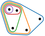
Figure 3: Hypergraph sub-structures in which the memoization of Algorithm 4 significantly improves the performance over that of Algorithm 3. On the left is the sunflower hypergraph where many edges share a common intersection, and on the right is the nested hypergraph where edges satisfy a containment relationship.

In spite of the difficulty in determining the exact number of convolutions saved by using the CCSS structure, we can still identify key substructures that lead to significant performance benefits; namely nested families of edges and “sunflowers” (collections of edges with a shared intersection), see Fig. 3. For example, with a nested series of edges $e_{1}\subset e_{2}\subset\cdots\subset e_{k}$, Algorithm 3 will require the computation of $\sum_{i=1}^{k}|e_{i}|^{2}-|e_{i}|$ convolutions without memoization. In contrast, the optimal CCSS tree will yield require only $\frac{|e_{k}|^{2}-|e_{k}|-2}{2}+\sum_{i=1}^{k}|e_{i}|$ convolutions. Similarly, if we consider a sunflower consisting of $m$ edges of size $k$ with a common intersection of size $t$, we can see that the non-memoized computation will require $m(k^{2}-k)$ convolution calculations while the memoized version requires

$$\frac{(k-t-1)^{2}+(k-t-1)}{2}+(t-2)t+(k-t)m+km$$

convolutions. In fact, even for a single edge of size $k$, the non-memoized computation requires at $k^{2}-k$ convolutions while the memoized version will require $\frac{k^{2}-k}{2}$. Thus the memoization decreases by a factor of at least 2 times the number of convolution operations necessary to evaluate S³TTVc.

V Experiments

We compare the runtime performance and thread scalability of our shared-memory parallel S³TTVc algorithm CCSS-MEMO against our two baseline approaches — CCSS-DIRECT and CCSS-FFT — for a collection of real-world and synthetic datasets.

V-A Platform and experimental configurations

Our experiments were conducted on a shared-memory machine with two 64-core AMD Epyc 7713 CPUs at 2.0 GHz and 512GB DDR4 DRAM. This work is implemented using C++ and multi-threading parallelized using OpenMP; all numerical operations are performed using double-precision floating point arithmetic and 64-bit unsigned integers. It is compiled using GCC 10.3.0 and Netlib LAPACK 3.8.0 [24] for linear algebra routines. The polynomial multiplication optimization is performed via full one-dimensional discrete convolution using Fast Fourier Transform (FFT) implementation from FFTW library [25].

V-B Datasets

We tested with eight real-world datasets and four synthetic datasets for more analysis, shown in Table I.

TABLE I: Summary of datasets.

Category	Symbol	Dataset	$|V|$	$|E|$	$N_{k}$	Ref.	Brief overview of dataset
Real-world	R1	MAG-10	80198	51889	25	[26, 27]	subset of coauthorship MicrosoftAcademic Graph
	R2	DAWN	2109	87104	22	[26]	drugs in patients prior to ER visit
	R3	cooking	6714	39774	65	[26]	recipes formed by combining different ingredients
	R4	walmart-trips	88860	69906	25	[26]	sets of co-purchased products at Walmart
	R5	trivago-clicks	172738	233202	86	[28]	sets of hotel accommodations clicked out by user
	R6	amazon-reviews	2193601	3685588	26	[29]	(filtered) sets of Amazon product reviews
	R7	mathoverflow	5176	39793	100	[30]	(filtered) sets of answers by Math Overflow users
	R8	stackoverflow	7816553	1047818	76	[30]	(filtered) sets of answers by Stack Overflow users
Synthetic	S1 S2 S3 S4	Synthetic 1 Synthetic 2 Synthetic 3 Synthetic 4	2500 2500 2500 2500	25000 25000 25000 25000	30 40 50 60	–	Randomly generated non-uniform hypergraphs consisting of 5-, 10-, 15-, … $N_{k}-$uniform hypergraphs, with each uniform hypergraph containing $|E|/k$ hyperedges uniformly chosen from all $\binom{|V|}{N_{l}}$ hyperedges, $1\leq l\leq k$

Real-world data. The real-world data come from diverse applications with different amount of nodes $|V|$ (ranging from $10^{3}$ to $10^{6}$), hyperedges $|E|$ (ranging from $10^{4}$ to $10^{6}$), and component adjacency tensors $N_{k}$ (ranging from 22–100). A brief introductory description and reference of the real-world datasets are given in the last two columns. Note that datasets which contain “filtered” in their description are filtered versions of the originals, using the less than or equal to filtering from Landry et al. [31] to remove all hyperedges of size larger than $N_{k}$.

Synthetic data. The synthetic datasets are random hypergraphs on the same set of nodes with the same total amount of hyperedges. But the hyperedges are of varying sizes, uniformly chosen at random over the vertex set. For each of S1, S2, S3 and S4, the component symmetric adjacency tensor orders were taken to be multiples of five until the hypergraph rank i.e. maximum component adjacency tensor order, with each component tensor containing approximately the same number of hyperedges.

V-C Overall performance

We evaluate the performance of both implementations of Algorithm 3, i.e., CCSS-DIRECT that directly computes the polynomial multiplication and CCSS-FFT that substitutes the polynomial multiplication kernel with a FFT convolution approach, and Algorithm 4 (CCSS-MEMO), which memoizes the coefficients to compute S³TTVc using a single traversal of the CCSS representation on both categories of datasets.

TABLE II: Single-core speedups of CCSS-DIRECT, CCSS-FFT, and CCSS-MEMO versus the Python implemented Algorithm 2 in [13].

speedup	R1	R2	R3	R4	R5	R6	R7	R8
CCSS-DIRECT	0.7	1.0	0.2	1.4	0.1	-	0.1	-
CCSS-FFT	2.4	3.5	2.8	4.2	0.4	4.7	2.1	2.6
CCSS-MEMO	2.4	5.2	3.0	17.0	1.3	18.6	4.5	4.6

Comparisons to SOTA methods. In Table II, we summarize the speedups of CCSS-DIRECT, CCSS-FFT, and CCSS-MEMO on a single core as compared to the state-of-the-art single-core Python implementation of Algorithm 2 [13]. Our CCSS-MEMO outperforms considerably, providing speedups of 1.3 – 18.6 times on the eight real-world datasets, while CCSS-FFT provides considerable improvements as well. CCSS-DIRECT largely underperforms, due to using direct convolution instead of FFT, with the exception being walmart-trips, where it obtains a speedup of 1.4. Although the timing results in Aksoy et al. [13] were obtained using a different language and system, the speedup observed is almost two orders of magnitude for the largest dataset, amazon-reviews, which suggests that the speedup is due to improvements in the algorithm as opposed to system and implementation differences. Further, as the dominate subroutine (the convolution operation) is implemented using optimized and compiled code (via a Python-wrapper in [13]) one would expect that much of the performance differences resulting from language choice are mitigated. Furthermore, the strong scaling results seen in Fig. 6 suggest even greater speedups as we increase the number of cores.

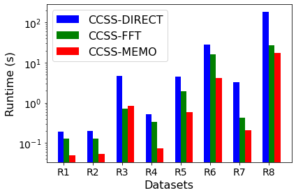
Figure 4: Overall runtime performance of CCSS-MEMO, CCSS-DIRECT and CCSS-FFT for real-world datasets in Table I

Real-world datasets. Fig. 4 presents the runtime performance on 128 cores of these three approaches for the real-world datasets. CCSS-MEMO performs the best on almost all the eight datasets, achieves $1.97-53.98\times$ speedup over CCSS-DIRECT and $0.65-12.45\times$ speedup over CCSS-FFT. The variation in speedups across different datasets for CCSS-MEMO is inherent to the hypergraph structure, and is due to the degree of overlap in the hyperedges present in the hypergraph. For the R3 dataset, we can see from Fig. 7 that CCSS achieves very low compression compared to the coordinate format. Thus, there is no significant advantage in using the memoization approach to compute S³TTVc, which is why we see that CCSS-FFT slightly outperforms CCSS-MEMO for higher thread configurations for this dataset.

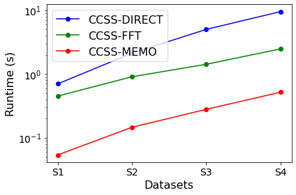
Figure 5: Comparison of runtime of CCSS-MEMO with CCSS-DIRECT and CCSS-FFT for synthetic datasets in Table I to highlight effect of rank of non-uniform hypergraph on S³TTVc computation.

Synthetic datasets. Since the synthetic datasets maintain the same number of IOU non-zeros across component uniform hypergraphs, the number of leaf nodes per level of the CCSS that contribute the S³TTVc computation is the same. This allows us to inspect the effect of the rank of the non-uniform hypergraph on the performance of all three algorithms. We see from Fig. 5 that sub-coefficient memoization has a significant impact on performance for hypergraphs of increasing ranks. This is to be expected since with increasing tensor order, the reduction in the number of traversals of the CCSS, as well as sharing of sub-coefficients between overlapping hyperedges for a uniform hyperedge distribution, would result in improved performance compared to CCSS-DIRECT and CCSS-FFT.

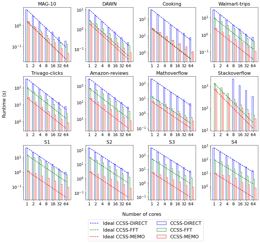
Figure 6: Thread scalability of CCSS-DIRECT, CCSS-FFT, and CCSS-MEMO for synthetic and real-world datasets in Table I. We set the time limit of our jobs at 50 minutes for all thread configurations. The stackoverflow dataset does not complete within the allotted time for 1, 2 and 4 thread configurations for CCSS-DIRECT.

V-D Thread scalability

Fig. 6 compares the thread scalability of CCSS-DIRECT, CCSS-FFT, and CCSS-MEMO for synthetic and real-world datasets in Table I. Across all datasets, we see that the CCSS-MEMO approach is faster than both the baseline approaches. The dashed lines indicate the ideal speedup lines for each of the three algorithms. CCSS-DIRECT and CCSS-FFT do not use memoization for the intermediate $\bar{E}_{N}(v)$ computations. The CCSS-DIRECT algorithm shows the best scalability of the three approaches, while both CCSS-FFT and CCSS-MEMO show decreasing scalability with increasing number of threads. For both of these approaches, as the work done per thread reduces (in terms of optimized FFT subroutines in FFTW for CCSS-FFT and in terms of coefficient $W$ memoization for CCSS-MEMO), the overhead in the atomic operation becomes more significant, especially for the hypergraphs with smaller number of nodes, and this manifests as suboptimal scaling. Moreover, the scalability of CCSS-MEMO is also affected by the load imbalance between threads due to the varying number of IOU non-zeros across trees within the CCSS structure.

Figure 7: Summary statistics for CCSS construction for representative datasets in Table I. We see that CCSS achieves more compact storage than the coordinate format i.e. storing the adjacency tensor non-zeros as lists of index tuples along with their non-zero value.

V-E CCSS Construction

CCSS construction. While the CSS compressed only in terms of overlapping IOU non-zeros within a symmetric adjacency tensor, the CCSS adds another layer of compactness in terms of shared indices between IOU non-zeros across multiple symmetric tensors. Moreover, for computing S³TTVc on the blowup tensor using the CCSS, we can further prune paths if the leaf node of the path does not own any IOU non-zeros. Fig. 7(a) shows the size of the constructed CCSS for representative synthetic and real-world datasets, while Fig. 7(b) examines the ratio of the amount of time spent in the construction of CCSS to the runtime of CCSS-MEMO for S³TTVc computation.

V-F $H$-eigenvector centrality computation speedups

CCSS-MEMO provides a practical framework to compute centrality in large hypergraphs. We compute tensor H-eigenvector centrality using Algorithm 1 on the largest real-world dataset in Table I — the amazon-reviews — on 128 cores. CCSS-MEMO obtains speedups of $6.49\times$ and $3.53\times$ over CCSS-DIRECT and CCSS-FFT respectively, which shows the applicability of this work in the analysis of real-world hypergraphs.

VI Conclusion

This work introduces the CCSS, an extension of the CSS for uniform hypergraphs, to compactly non-uniform hypergraphs. A novel memoization-based algorithm CCSS-MEMO adapted from the generating function approach is proposed to compute S³TTVc on the blowup adjacency tensor of non-uniform hypergraphs. We demonstrate the performance of our shared-memory parallel CCSS-MEMO by comparing it to two naive baseline algorithms using the CCSS - CCSS-DIRECT and CCSS-FFT - for multiple synthetic and real-world datasets. In the future, we plan to explore distributed-memory construction of CCSS and distributed-memory parallel S³TTVc computation using CCSS-MEMO. Furthermore, we plan to utilize CCSS-MEMO as the computational kernel in extending multilinear PageRank to nonuniform hypergraphs, where we anticipate its advanced data structures and parallelization will allow analysis of datasets previously considered prohibitively large for tensor analysis. Our fast algorithm would also help facilitate the multilinear hypergraph clustering  [13]. Moreover, we believe it opens the door for development of tensor-based methods for semi-supervised and supervised hypergraph learning tasks such as node classification and link prediction.

References

- [1] Y. Yamaguchi, A. Ogawa, A. Takeda, and S. Iwata, “Cyber security analysis of power networks by hypergraph cut algorithms,” 2014 IEEE International Conference on Smart Grid Communications, SmartGridComm 2014, pp. 824–829, 1 2015.
- [2] C. A. Joslyn, S. Aksoy, D. Arendt, J. Firoz, L. Jenkins, B. Praggastis, E. Purvine, and M. Zalewski, “Hypergraph Analytics of Domain Name System Relationships,” in Algorithms and Models for the Web Graph, B. Kamiński, P. Prałat, and P. Szufel, Eds. Cham: Springer International Publishing, 2020, pp. 1–15.
- [3] S. Feng, E. Heath, B. Jefferson, C. Joslyn, H. Kvinge, H. D. Mitchell, B. Praggastis, A. J. Eisfeld, A. C. Sims, L. B. Thackray, S. Fan, K. B. Walters, P. J. Halfmann, D. Westhoff-Smith, Q. Tan, V. D. Menachery, T. P. Sheahan, A. S. Cockrell, J. F. Kocher, K. G. Stratton, N. C. Heller, L. M. Bramer, M. S. Diamond, R. S. Baric, K. M. Waters, Y. Kawaoka, J. E. McDermott, and E. Purvine, “Hypergraph models of biological networks to identify genes critical to pathogenic viral response,” BMC Bioinformatics, vol. 22, no. 1, pp. 1–21, 12 2021. [Online]. Available: https://bmcbioinformatics.biomedcentral.com/articles/10.1186/s12859-021-04197-2
- [4] J. Zhu, J. Zhu, S. Ghosh, W. Wu, and J. Yuan, “Social Influence Maximization in Hypergraph in Social Networks,” IEEE Transactions on Network Science and Engineering, vol. 6, no. 4, pp. 801–811, 10 2019.
- [5] A. Ganesan, “Structured Hypergraphs in Cellular Mobile Communication Systems,” ACM International Conference Proceeding Series, pp. 188–196, 1 2023. [Online]. Available: https://dl.acm.org/doi/10.1145/3571306.3571335
- [6] A. R. Benson, D. F. Gleich, and J. Leskovec, “Tensor Spectral Clustering for Partitioning Higher-order Network Structures,” SIAM International Conference on Data Mining 2015, SDM 2015, pp. 118–126, 2 2015. [Online]. Available: http://arxiv.org/abs/1502.05058http://dx.doi.org/10.1137/1.9781611974010.14
- [7] Z. T. Ke, F. Shi, and D. Xia, “Community Detection for Hypergraph Networks via Regularized Tensor Power Iteration,” 2020.
- [8] X. Ouvrard, J. M. Le Goff, and S. Marchand-Maillet, “On Adjacency and e-Adjacency in General Hypergraphs: Towards a New e-Adjacency Tensor,” Electronic Notes in Discrete Mathematics, vol. 70, pp. 71–76, 12 2018.
- [9] Y. Zhen and J. Wang, “Community Detection in General Hypergraph via Graph Embedding,” Journal of the American Statistical Association, 3 2021. [Online]. Available: https://arxiv.org/abs/2103.15035v2
- [10] I. Dumitriu, H. Wang, and Y. Zhu, “Partial recovery and weak consistency in the non-uniform hypergraph Stochastic Block Model,” 12 2021. [Online]. Available: https://arxiv.org/abs/2112.11671v2
- [11] I. Dumitriu and H. Wang, “Exact recovery for the non-uniform Hypergraph Stochastic Block Model,” 4 2023. [Online]. Available: https://arxiv.org/abs/2304.13139v1
- [12] A. Banerjee, A. Char, and B. Mondal, “Spectra of general hypergraphs,” Linear Algebra and its Applications, vol. 518, pp. 14–30, 2017. [Online]. Available: https://www.sciencedirect.com/science/article/pii/S0024379516306115
- [13] S. G. Aksoy, I. Amburg, and S. J. Young, “Scalable tensor methods for nonuniform hypergraphs,” 2023.
- [14] T. G. Kolda, “Numerical optimization for symmetric tensor decomposition,” Mathematical Programming, vol. 151, no. 1, pp. 225–248, 4 2015.
- [15] T. G. Kolda and J. R. Mayo, “Shifted Power Method for Computing Tensor Eigenpairs,” https://doi.org/10.1137/100801482, vol. 32, no. 4, pp. 1095–1124, 10 2011. [Online]. Available: https://epubs.siam.org/doi/10.1137/100801482
- [16] T. G. Kolda, “Symmetric Orthogonal Tensor Decomposition is Trivial,” 3 2015. [Online]. Available: https://arxiv.org/abs/1503.01375v1
- [17] A. R. Benson, “Three Hypergraph Eigenvector Centralities,” SIAM Journal on Mathematics of Data Science, vol. 1, no. 2, pp. 293–312, 2019. [Online]. Available: https://doi.org/10.1137/18M1203031
- [18] S. Shivakumar, J. Li, R. Kannan, and S. Aluru, “Efficient Parallel Sparse Symmetric Tucker Decomposition for High-Order Tensors,” in Proceedings of the 2021 SIAM Conference on Applied and Computational Discrete Algorithms (ACDA21), 2021, pp. 193–204. [Online]. Available: https://epubs.siam.org/doi/abs/10.1137/1.9781611976830.18
- [19] ——, “Sparse Symmetric Format for Tucker Decomposition,” IEEE Transactions on Parallel and Distributed Systems, vol. 34, no. 6, pp. 1743–1756, 2023.
- [20] T. G. Kolda and B. W. Bader, “Tensor Decompositions and Applications,” SIAM Review, vol. 51, no. 3, pp. 455–500, 2009. [Online]. Available: https://doi.org/10.1137/07070111X
- [21] M. Ng, L. Qi, and G. Zhou, “Finding the Largest Eigenvalue of a Nonnegative Tensor,” SIAM Journal on Matrix Analysis and Applications, vol. 31, no. 3, pp. 1090–1099, 2010. [Online]. Available: https://doi.org/10.1137/09074838X
- [22] H. S. Wilf, Generatingfunctionology, third edition ed. USA: A. K. Peters/CRC Press, 2006. [Online]. Available: https://doi.org/10.1201/b10576
- [23] James W Cooley and John W Tukey, “An algorithm for the machine calculation of complex Fourier series,” Mathematics of computation, vol. 19, no. 90, pp. 297–301, 1965.
- [24] E. Anderson, Z. Bai, C. Bischof, L. S. Blackford, J. Demmel, J. Dongarra, J. Du Croz, A. Greenbaum, S. Hammarling, A. McKenney, and others, LAPACK users’ guide. SIAM, 1999.
- [25] M. Frigo and S. G. Johnson, “The Design and Implementation of FFTW3,” Proceedings of the IEEE, vol. 93, no. 2, pp. 216–231, 2005.
- [26] I. Amburg, N. Veldt, and A. Benson, “Clustering in Graphs and Hypergraphs with Categorical Edge Labels,” in Proceedings of The Web Conference 2020, ser. WWW ’20. New York, NY, USA: Association for Computing Machinery, 2020, pp. 706–717. [Online]. Available: https://doi.org/10.1145/3366423.3380152
- [27] A. Sinha, Z. Shen, Y. Song, H. Ma, D. Eide, B.-J. P. Hsu, and K. Wang, “An Overview of Microsoft Academic Service (MAS) and Applications,” in Proceedings of the 24th International Conference on World Wide Web, ser. WWW ’15 Companion. New York, NY, USA: Association for Computing Machinery, 2015, pp. 243–246. [Online]. Available: https://doi.org/10.1145/2740908.2742839
- [28] P. S. Chodrow, N. Veldt, and A. R. Benson, “Hypergraph clustering: from blockmodels to modularity,” Science Advances, 2021.
- [29] J. Ni, J. Li, and J. McAuley, “Justifying Recommendations using Distantly-Labeled Reviews and Fine-Grained Aspects,” in Proceedings of the 2019 Conference on Empirical Methods in Natural Language Processing and the 9th International Joint Conference on Natural Language Processing (EMNLP-IJCNLP), 2019, pp. 188–197. [Online]. Available: https://www.aclweb.org/anthology/D19-1018
- [30] N. Veldt, A. R. Benson, and J. Kleinberg, “Minimizing Localized Ratio Cut Objectives in Hypergraphs,” in Proceedings of the 26th ACM SIGKDD International Conference on Knowledge Discovery & Data Mining, ser. KDD ’20. New York, NY, USA: Association for Computing Machinery, 2020, pp. 1708–1718. [Online]. Available: https://doi.org/10.1145/3394486.3403222
- [31] N. W. Landry, I. Amburg, M. Shi, and S. G. Aksoy, “Filtering higher-order datasets,” arXiv preprint arXiv:2305.06910, 2023.