A solver for linear scalar ordinary differential equations whose running time is bounded independent of frequency

Abstract

When the eigenvalues of the coefficient matrix for a linear scalar ordinary differential equation are of large magnitude, its solutions exhibit complicated behaviour, such as high-frequency oscillations, rapid growth or rapid decay. The cost of representing such solutions using standard techniques grows with the magnitudes of the eigenvalues. As a consequence, the running times of most solvers for ordinary differential equations also grow with these eigenvalues. However, a large class of scalar ordinary differential equations with slowly-varying coefficients admit slowly-varying phase functions that can be represented at a cost which is bounded independent of the magnitudes of the eigenvalues of the corresponding coefficient matrix. Here, we introduce a numerical algorithm for constructing slowly-varying phase functions which represent the solutions of a linear scalar ordinary differential equation. Our method’s running time depends on the complexity of the equation’s coefficients, but is bounded independent of the magnitudes of the equation’s eigenvalues. Once the phase functions have been constructed, essentially any reasonable initial or boundary value problem for the scalar equation can be easily solved. We present the results of numerical experiments showing that, despite its greater generality, our algorithm is competitive with state-of-the-art methods for solving highly-oscillatory second order differential equations. We also compare our method with Magnus-type exponential integrators and find that our approach is orders of magnitude faster in the high-frequency regime.

1 Introduction

The complexity of the solutions of an $n^{th}$ order linear homogeneous ordinary differential equation

$$y^{(n)}(t)+q_{n-1}(t)y^{(n-1)}(t)+\cdots+q_{1}(t)y^{\prime}(t)+q_{0}(t)y(t)=0$$ (1)

increases with the magnitudes of the eigenvalues $\lambda_{1}(t),\ldots,\lambda_{n}(t)$ of the coefficient matrix

$$\left(\begin{array}[]{cccccccc}0&1&0&\cdots&0&0\\ 0&0&1&\cdots&0&0\\ \vdots&&&\ddots&&\vdots\\ 0&0&0&\cdots&1&0\\ 0&0&0&\cdots&0&1\\ -q_{0}(t)&-q_{1}(t)&-q_{2}(t)&\cdots&-q_{n-2}(t)&-q_{n-1}(t)\\ \end{array}\right)$$ (2)

obtained from (1) in the usual way. Indeed, the cost to represent such solutions over an interval $[a,b]$ using standard techniques (e.g., polynomial or trigonometric expansions) typically grows roughly linearly with the quantity

$$\Omega=\max_{i=1,\ldots,n}\int_{a}^{b}\left|\lambda_{i}(t)\right|\,dt,$$ (3)

which we refer to as the frequency of (1). We use this terminology because, in most cases of interest, it is the imaginary parts of the eigenvalues which are of large magnitude. Indeed, when the real part of one or more of the $\lambda_{j}(t)$ is large in size, most initial and terminal value problems for (1) are highly ill-conditioned and solving them numerically requires specialized techniques which exploit additional information about the desired solution.

Although the complexity of the solutions of (1) increases with frequency, a large class of linear scalar ordinary differential equations admit phase functions whose cost to represent via standard techniques is bounded independent of the magnitudes of the eigenvalues of (2). In fact, if $q_{0},\ldots,q_{n-1}$ are slowly-varying on an interval $I$ and the differential equation (1) is nondegenerate there — meaning that the eigenvalues $\lambda_{1}(t),\ldots,\lambda_{n}(t)$ are distinct for each $t\in I$ — then it is possible to find slowly-varying phase functions $\psi_{1},\ldots,\psi_{n}\colon I\to\mathbb{C}$ such that

$$\left\{\exp\left(\psi_{j}(t)\right):j=1,\ldots,n\right\}$$ (4)

is a basis for the space of solutions of (1) given on the interval $I$. That slowly-varying phase functions exist under these conditions, at least in an asymptotic sense, has long been known. Indeed, this observation is the basis of the WKB method and other related techniques (see, for instance, Miller , Wasov and SpiglerPhase1 ; SpiglerPhase2 ; SpiglerZeros ). A theorem which establishes the existence of slowly-varying phase functions for second order differential equations under mild conditions on their coefficients is proven in BremerRokhlin . Although it is not immediately obvious how to generalize the argument of BremerRokhlin to higher order scalar equations, known results regarding the asymptotic approximation of solutions of differential equations and numerical evidence (including the experiments of this paper) strongly suggest the situation for higher order scalar equations is much the same as it is for second order equations.

The derivatives of the phase functions $\psi_{1},\ldots,\psi_{n}$, which we denote by $r_{1},\ldots,r_{n}$, satisfy an $(n-1)^{st}$ order nonlinear inhomogeneous ordinary differential equation, the general form of which is quite complicated. When $n=2$, it is the Riccati equation

$$r^{\prime}(t)+(r(t))^{2}+q_{1}(t)r(t)+q_{0}(t)=0;$$ (5)

when $n=3$, the nonlinear equation is

$$r^{\prime\prime}(t)+3r^{\prime}(t)r(t)+(r(t))^{3}+q_{2}(t)r^{\prime}(t)+q_{2}(t)(r(t))^{2}+q_{1}(t)r(t)+q_{0}(t)=0;$$ (6)

and, for $n=4$, we have

$$r^{\prime\prime\prime}(t) +4r^{\prime\prime}(t)r(t)+3(r^{\prime}(t))^{2}+6r^{\prime}(t)(r(t))^{2}+(r(t))^{4}+q_{3}(t)(r(t))^{3}+q_{3}(t)r^{\prime\prime}(t)$$ (7)

$$+3q_{3}(t)r^{\prime}(t)r(t)+q_{2}(t)(r(t))^{2}+q_{2}(t)r^{\prime}(t)+q_{1}(t)r(t)+q_{0}(t)=0.$$

By a slight abuse of terminology, we will refer to the $(n-1)^{st}$ order nonlinear equation obtained by inserting the representation

$$y(t)=\exp\left(\int r(t)\,dt\right)$$ (8)

into (1) as the $(n-1)^{st}$ order Riccati equation, or, alternatively, the Riccati equation for (1).

An obvious approach to initial and boundary value boundary problems for (1) calls for constructing a suitable collection of slowly-varying phase functions by solving the corresponding Riccati equation numerically. Doing so is not as straightforward as it sounds, however. The principal difficulty is that most solutions of the Riccati equation for (1) are rapidly-varying when the eigenvalues $\lambda_{1}(t),\ldots,\lambda_{n}(t)$ are of large magnitude, and some mechanism is needed to select the slowly-varying solutions.

The article BremerPhase introduces an algorithm for constructing two slowly-varying phase function $\psi_{1}$ and $\psi_{2}$ such that $\exp(\psi_{1}(t))$ and $\exp(\psi_{2}(t))$ constitute a basis in the space of solutions of a second order linear ordinary differential equation of the form

$$y^{\prime\prime}(t)+q(t)y(t)=0,\ \ \ \ \ a<t<b,$$ (9)

where $q$ is slowly-varying and non-vanishing on $(a,b)$. It operates by constructing a smoothly deformed version of the coefficient $q$ which is equal to an appropriately chosen constant in a neighborhood of some point $c$ in $(a,b)$ and coincides with the original coefficient $q$ in a neighborhood of a point $d$ in $(a,b)$. There is a pair of slowly-varying phase functions for the deformed equation whose derivatives at $c$ are known and whose derivatives at $d$ coincide with the derivatives of a pair of slowly-varying phase functions for the original equation. Consequently, by solving the Riccati equation corresponding to the deformed equation with initial conditions specified at $c$, the values of the derivatives of a pair of slowly-varying phase functions for the original equation at the point $d$ can be calculated. Once this has been done, the Riccati equation corresponding to the original equation is solved using the values at $d$ as initial conditions in order to calculate the derivatives of a pair of slowly-varying phase functions for (9) over the whole interval. The desired slowly-varying phase functions $\psi_{1}$ and $\psi_{2}$ are obtained by integration. The cost of the entire procedure is bounded independent of the magnitude of $q$, which is related to the eigenvalues of the coefficient matrix corresponding to (9) via

$$\lambda_{1}(t)=\sqrt{-q(t)}\ \ \ \mbox{and}\ \ \ \lambda_{2}(t)=-\sqrt{-q(t)}.$$ (10)

From (10), it follows that the assumption that $q$ is non-vanishing on $(a,b)$ is equivalent to the condition that (9) is nondegenerate on $(a,b)$. In BremerPhase2 , the method of BremerPhase is extended to the case in which (9) is nondegenerate on an interval $[a,b]$ except at a finite number of turning points. The equation (1) has a turning point at $t_{0}$ provided the eigenvalues $\lambda_{1}(t),\ldots,\lambda_{n}(t)$ of (2) are distinct in a deleted neighborhood of $t_{0}$, but coalesce at $t_{0}$. The turning points of (9), then, are precisely the isolated zeros of $q$. Because slowly-varying phase functions need not extend across turning points, the algorithm of BremerPhase2 introduces a partition $a=\xi_{1}<\xi_{2}<\ldots<\xi_{k}=b$ of $[a,b]$ such that $\xi_{2},\ldots,\xi_{k-1}$ are the roots of $q$ in the open interval $(a,b)$. It then applies a variant of the method of BremerPhase to each of the subintervals $\left[\xi_{j},\xi_{j+1}\right]$, $j=1,\ldots,k-1$, which results in a collection of $2(k-1)$ slowly-varying phase functions that efficiently represent the solutions of (9).

It is relatively straightforward to generalize the approach of BremerPhase to the case of nondegenerate higher order scalar equations. However, while the resulting algorithm is highly-effective for a large class of equations of the form (1), the authors have found another approach inspired by the classical Levin method for evaluating oscillatory integrals to be somewhat more robust. Introduced in Levin , the Levin method is based on the observation that if $p_{0}$ and $f$ are slowly varying, then the inhomogeneous equation

$$y^{\prime}(t)+p_{0}(t)y(t)=f(t)$$ (11)

has a slowly-varying solution $y_{0}$, regardless of the magnitude of $p_{0}$. Similarly to the case of phase functions, the proofs appearing in Levin and subsequent works on the Levin method do not immediately apply to the case of higher order scalar equations, but experimental evidence and results for special cases strongly suggest that the Levin principle generalizes. That is to say, equations of the form

$$y^{(n)}(t)+p_{n-1}(t)y^{(n-1)}(t)+\cdots+p_{1}(t)y^{\prime}(t)+p_{0}(t)y(t)=f(t).$$ (12)

admit solutions whose complexity depends on that of the right-hand side $f$ and of the coefficients $p_{0},\ldots,p_{n-1}$, but is bounded independent of the magnitudes of $p_{0},\ldots,p_{n-1}$.

The algorithm of this paper exploits the existence of slowly-varying phase functions and the Levin principle to solve initial and boundary value problems for nondegenerate scalar equations of the form (1) with slowly-varying coefficients. It operates by constructing slowly-varying phase functions $\psi_{1}\ldots,\psi_{n}$ such that (4) is a basis in the space of solutions of a nondegenerate scalar equation. Once this has been done, any reasonable initial or boundary value problem for (1) can be solved more-or-less instantaneously. As with BremerPhase , the method of this paper can be extended to the case of a scalar equation which is nondegenerate on an interval $[a,b]$ except at a finite number of turning points by applying it on a collection of subintervals of $[a,b]$; however, for the sake of simplicity, we consider only nondegenerate equations here.

The algorithms of BremerPhase , BremerPhase2 and this article bear some superficial similarities to Magnus expansion methods. Introduced in Magnus , Magnus expansions are certain series of the form

$$\sum_{k=1}^{\infty}\Omega_{k}(t)$$ (13)

such that $\exp\left(\sum_{k=1}^{\infty}\Omega_{k}(t)\right)$ locally represents a fundamental matrix for a system of differential equations

$$\mathbf{y}^{\prime}(t)=A(t)\mathbf{y}(t).$$ (14)

The first few terms for the series around $t=0$ are given by

$$\Omega_{1}(t) =\int_{0}^{t}A(s)\ ds,$$ (15)

$$\Omega_{2}(t) =\frac{1}{2}\int_{0}^{t}\int_{0}^{t_{1}}\left[A(t_{1}),A(t_{2})\right]\,dt_{2}dt_{1}\ \ \ \mbox{and}$$

$$\Omega_{3}(t) =\frac{1}{6}\int_{0}^{t}\int_{0}^{t_{1}}\int_{0}^{t_{2}}\left[A(t_{1}),\left[A(t_{2}),A(t_{3})\right]\right]+\left[A(t_{3}),\left[A(t_{2}),A(t_{1})\right]\right]\,dt_{3}dt_{2}dt_{1}.$$

The straightforward evaluation of the $\Omega_{j}$ is nightmarishly expensive; however, a clever technique which renders the calculations manageable is introduced in Iserles101 and it paved the way for the development of a class of numerical solvers which represent a fundamental matrix for (14) over an interval $I$ via a collection of truncated Magnus expansions. While the entries of the $\Omega_{j}$ are slowly-varying whenever the entries of $A(t)$ are slowly-varying, the radius of convergence of the series in (13) depends on the magnitude of the coefficient matrix $A(t)$, which is, in turn, related to the magnitudes of the eigenvalues of $A(t)$. Of course, this means that the number of Magnus expansions which are needed to solve a given problem, and hence the cost of the method, grows with the magnitudes of the eigenvalues of $A(t)$. See, for instance, Iserles102 , which gives for estimates of the growth in the running time of Magnus expansion methods in the case of an equation of the form (9) as a function of the magnitude of the coefficient $q$.

Nonetheless, Magnus expansion methods are much more efficient than standard solvers for ordinary differential equations in the high-frequency regime. Indeed, exponential integrators which approximate Magnus expansions while avoiding the explicit calculation of commutators (those discussed in Blanes3 , for instance) appear to be the current state-of-the-art approach to solving scalar ordinary differential equations of order three or higher. In our experiments, we compare our method against $4^{th}$ and $6^{th}$ order “classical” Magnus methods which explicitly make use of commutators, as well as $4^{th}$ and $6^{th}$ order commutator-free quasi-Magnus exponential integrators. Since the running time of our algorithm is largely independent of frequency, our method is orders of magnitude faster than Magnus-type methods in the high-frequency regime. Perhaps surprisingly, we find that it is also faster even at quite low frequencies. We note, though, that Magnus expansion methods are more general than our method in that they apply to systems of linear ordinary differential equations and not just scalar equations. Our experiment comparing our approach with Magnus-type methods is described in Subsection 5.2.

We also compare our method with two specialized algorithms for second order equations: the smooth deformation method of BremerPhase (which was developed by one of the authors of this paper) and the ARDC method of agocs . These represent current state-of-the-art approaches to solving second order equations in the high-frequency regime. In the comparison made in Subsection 5.1, we find that, despite its much greater generality, the algorithm of this paper is only slightly slower than that of BremerPhase and it is as much as 15 times faster than the ARDC method of agocs .

The remainder of this article is organized as follows. In Section 2, we discuss the results of BremerRokhlin pertaining to the existence of slowly-varying phase functions for second order linear ordinary differential equations. Section 3 describes how the Levin principle can be exploited to compute these slowly-varying phase functions. In Section 4, we detail our numerical algorithm. The results of numerical experiments demonstrating the properties of our algorithm are discussed in Section 5. These experiments include comparisons with state-of-the-art methods for the special case of second order linear ordinary differential equations and with Magnus-type exponential integrators. We briefly comment on the algorithm of this article and directions for future work in Section 6. Appendix A details a standard adaptive spectral solver for ordinary differential equations which is used by our algorithm and to construct reference solutions in our numerical experiments.

2 Slowly-varying phase functions for second order equations

Here, we briefly discuss the results of BremerRokhlin , which pertain to second order equations of the form

$$y^{\prime\prime}(t)+\omega^{2}q_{0}(t)y(t)=0,\ \ \ \ \ a<t<b,$$ (16)

with $q_{0}$ smooth and positive. Under these assumptions, the solutions of (16) are oscillatory, with the frequency of their oscillations controlled by the parameter $\omega$. Analogous results hold when $q_{0}$ is negative and the solutions of (16) are combinations of rapidly increasing and decreasing functions. It is not obvious, however, how to apply the argument of BremerRokhlin to higher order scalar equations. Nonetheless, there are strong indications, including relevant well-known results in asymptotic analysis (see, for instance, Wasov ) and experimental evidence, that the situation for higher order scalar equations is similar.

If $y(t)=\exp(\psi(t))$ satisfies (16), then it can be trivially verified that $\psi$ solves the Riccati equation

$$\psi^{\prime\prime}(t)+\left(\psi^{\prime}(t)\right)^{2}+\omega^{2}q_{0}(t)=0.$$ (17)

By inserting the expression $\psi(t)=i\alpha(t)+\beta(t)$ into (17), we see that if $\alpha$ and $\beta$ satisfy the system of equations

$$\left\{\begin{aligned} \beta^{\prime\prime}(t)+(\beta^{\prime}(t))^{2}-(\alpha^{\prime}(t))^{2}+\omega^{2}q_{0}(t)&=0\\ \alpha^{\prime\prime}(t)+2\alpha^{\prime}(t)\beta^{\prime}(t)&=0,\end{aligned}\right.$$ (18)

then $\psi$ solves (17). The second equation in (18) admits the formal solution

$$\beta(t)=-\frac{1}{2}\log(\alpha^{\prime}(t)),$$ (19)

so that $\psi$ can be written in the form

$$\psi(t)=i\alpha(t)-\frac{1}{2}\log\left(\alpha^{\prime}(t)\right).$$ (20)

Because of the close relationship between $\alpha$ and $\psi$, both are referred to as phase functions for (16). Moreover, a bound on the complexity of one readily gives a bound on the complexity of the other.

Inserting (19) into the first equation in (18) yields

$$\omega^{2}q_{0}(t)-(\alpha^{\prime}(t))^{2}+\frac{3}{4}\left(\frac{\alpha^{\prime\prime}(t)}{\alpha^{\prime}(t)}\right)^{2}-\frac{1}{2}\frac{\alpha^{\prime\prime\prime}(t)}{\alpha^{\prime}(t)}=0.$$ (21)

Equation (21) is known as Kummer’s equation, after E. E. Kummer, who studied it in Kummer . The theorem of BremerRokhlin applies when the function $p(x)=\widetilde{p}(t(x))$, where $\widetilde{p}(t)$ is defined via

$$\widetilde{p}(t)=\frac{1}{\omega^{2}q_{0}(t)}\left(\frac{5}{4}\left(\frac{q_{0}^{\prime}(t)}{q_{0}(t)}\right)^{2}-\frac{q_{0}^{\prime\prime}(t)}{q_{0}(t)}\right)$$ (22)

and $t(x)$ is the inverse function of

$$x(t)=\int_{a}^{t}\sqrt{q_{0}(s)}\ ds,$$ (23)

has a rapidly decaying Fourier transform. More explicitly, the theorem asserts that if the Fourier transform of $p$ satisfies a bound of the form

$$\left|\widehat{p}(\xi)\right|\leq\Gamma\exp\left(-\mu\left|\xi\right|\right),$$ (24)

then there exist functions $\nu$ and $\delta$ such that

$$\left|\nu(t)\right|\leq\frac{\Gamma}{2\mu}\left(1+\frac{4\Gamma}{\omega}\right)\exp(-\mu\omega),$$ (25)

$$\left|\widehat{\delta}(\xi)\right|\leq\frac{\Gamma}{\omega^{2}}\left(1+\frac{2\Gamma}{\omega}\right)\exp(-\mu|\xi|)$$ (26)

and

$$\alpha(t)=\omega\sqrt{q_{0}(t)}\int_{a}^{t}\exp\left(\frac{\delta(u)}{2}\right)\ du$$ (27)

is a phase function for

$$y^{\prime\prime}(t)+\omega^{2}\left(q_{0}(t)+\frac{\nu(t)}{4\omega^{2}}\right)y(t)=0.$$ (28)

Because the magnitude of $\nu$ decays exponentially fast in $\omega$, Equation (28) is identical to (16) for the purposes of numerical computation when $\omega$ is of even very modest size. The definition of the function $p(x)$ is ostensibly quite complicated; however, $p(x)$ is, in fact, simply a constant multiple of Schwarzian derivative of the inverse function $t(x)$ of (23).

This result ensures that for all values of $\omega$, (16) admits a phase function which is slowly-varying. In the low-frequency regime, when $\omega$ is small, it can be the case that all phase functions for (16) oscillate, but they do so at low frequencies because $\omega$ is small. Once $\omega$ becomes sufficiently large, the function $\nu$ is vanishingly small, and the phase function associated with (28) is, at least for the purposes of numerical computation, a slowly-varying phase function for the original equation (16). Since $\nu$ decays exponentially fast in $\omega$, this happens at extremely modest frequencies.

Because of this phenomenon, in the low-frequency regime, the running time of numerical algorithms based on phase functions tend to grow with frequency. However, once a certain frequency threshold is reached, the complexity of the phase functions becomes essentially independent of frequency, or even slowly decreasing with frequency. This phenomenon can be clearly seen in all of the numerical experiments of this paper presented in Section 5.

3 The Levin approach to solving nonlinear ordinary differential equations

In its original application to oscillatory integrals, Levin’s principle was used to construct slowly-varying solutions to inhomogeneous linear ordinary differential equations. However, it can also be exploited to construct slowly-varying solutions of nonlinear ordinary differential equations, specifically the $(n-1)^{st}$ order Riccati equation.

When Newton’s method is applied to the $(n-1)^{st}$ order Riccati equation corresponding to (1), the result is a sequence of linearized equations of the form

$$y^{(n-1)}(t)+p_{n-2}(t)y^{(n-2)}(t)+\cdots+p_{1}(t)y^{\prime}(t)+p_{0}(t)y(t)=f(t).$$ (29)

Assuming the coefficients $q_{0},\ldots,q_{n-1}$ and the the initial guess used to initiate the Newton procedure are slowly-varying, the coefficients $p_{0},\ldots,p_{n-2}$ and the right-hand side $f$ appearing in the first linearized equation of the form (29) which arises will also be slowly-varying. According to the Levin principle that equation admits slowly-varying solutions. If such a solution is used to update the initial guess, then the second Newton iterate will also be slowly-varying and the second linear inhomogeneous equation which arises will have slowly-varying coefficients and a slowly-varying right-hand side. Continuing in this fashion results in a series of linearized equations of the form (12), all of which have slowly-varying coefficients and slowly-varying right-hand sides. Consequently, a slowly-varying solution of the Riccati equation can be constructed via Newton’s method as long as an appropriate slowly-varying initial guess is known.

Conveniently enough, there is an obvious mechanism for generating $n$ slowly-varying initial guesses for the $(n-1)^{st}$ order Riccati equation. In particular, the eigenvalues $\lambda_{1}(t),\ldots,\lambda_{n}(t)$ of the matrix (2), which are often used as low-accuracy approximations of solutions of the Riccati equation in asymptotic methods, are suitable as initial guesses for the Newton procedure.

Complicating matters slightly is the fact that the differential operator

$$D\left[y\right](t)=y^{(n-1)}(t)+p_{n-2}(t)y^{(n-2)}(t)+\cdots+p_{1}(t)y^{\prime}(y)+p_{0}(t)y(t)$$ (30)

appearing on the left-hand side of (29) admits a nontrivial nullspace which can contain rapidly-varying functions when one or more of the $p_{j}$ is of large magnitude. It is a central observation of Levin-type methods, however, that when (29) admits slowly-varying solutions along with rapidly-varying ones, a slowly-varying solution can be accurately and rapidly computed provided some case is taken. In particular, as long as one uses a Chebyshev spectral collocation scheme which is sufficient to resolve the coefficients $p_{0},\ldots,p_{n-1}$ as well as the right-hand side $f$ and the resulting linear system is solved via a truncated singular value decomposition, a high-accuracy approximation of a slowly-varying solution of (29) is obtained. Critically, the discretization need not be sufficient to resolve the rapidly-varying solutions of (29) so that the cost of solving the equation depends only on the complexity of the desired slowly-varying solution, rather than on the complexity of the rapidly-varying elements of the nullspace of (30). Numerical evidence to this effect in the case $n=2$ is provided in LevinLi and LiImproved , and a detailed analysis is given in SerkhBremerLevin .

4 Numerical Algorithm

In this section, we describe our method for the construction of a collection of slowly-varying phase functions $\psi_{1},\ldots,\psi_{n}$ such that (4) is a basis in the space of solutions of a nondegenerate equation of the form (1) with slowly-varying coefficients. Once these phase functions have been constructed, any reasonable initial or boundary value problem for (1) can be easily solved. Recall that we use $r_{1},\ldots,r_{n}$ to denote the first derivatives of the phase functions $\psi_{1},\ldots,\psi_{n}$.

The algorithm operates in two stages, each of which is detailed in a subsection below. In the first stage, the Levin principle is used to find the values of $r_{1},\ldots,r_{n}$ and their derivatives up to order $(n-2)$ at a point in the solution domain of the scalar equation. In the second stage, the Riccati equation corresponding to (1) is solved using these values as initial conditions in order to calculate $r_{1},\ldots,r_{n}$ and their derivatives through order $(n-2)$ over the entire solution interval and the phase functions $\psi_{1},\ldots,\psi_{n}$ are obtained by integrating $r_{1},\ldots,r_{n}$.

Our algorithm takes as input the following:

1. the interval $[a,b]$ over which the equation is given;

2. an external subroutine for evaluating the coefficients $q_{0},\ldots,q_{n-1}$ in (1);

3. a subinterval $[a_{0},b_{0}]$ of $[a,b]$ over which the Levin procedure is to be applied and a point $\sigma$ in that interval;

4. a point $\eta$ on the interval $[a,b]$ and the desired values $\psi_{1}(\eta),\ldots,\psi_{n}(\eta)$ for the phase functions at that point;

5. an integer $k$ which controls the order of the piecewise Chebyshev expansions used to represent the phase functions and their derivatives; and

6. a parameter $\epsilon$ which specifies the desired accuracy for the solutions of the Riccati equation computed in the second stage of the algorithm.

The output of our algorithm comprises $n^{2}$ piecewise Chebyshev expansions of order $(k-1)$, representing the phase functions $\psi_{1},\ldots,\psi_{n}$ and their derivatives through order $(n-1)$. To be entirely clear, by a $(k-1)^{st}$ order piecewise Chebyshev expansions on the interval $[a,b]$, we mean a sum of the form

$$\sum_{i=1}^{m-1}\chi_{\left[x_{i-1},x_{i}\right)}(t)\sum_{j=0}^{k-1}\lambda_{ij}\ T_{j}\left(\frac{2}{x_{i}-x_{i-1}}t+\frac{x_{i}+x_{i-1}}{x_{i}-x_{i-1}}\right)$$ (31)

$$+ \chi_{\left[x_{m-1},x_{m}\right]}(t)\sum_{j=0}^{k-1}\lambda_{mj}\ T_{j}\left(\frac{2}{x_{m}-x_{m-1}}t+\frac{x_{m}+x_{m-1}}{x_{m}-x_{m-1}}\right),$$

where $a=x_{0}<x_{1}<\cdots<x_{m}=b$ is a partition of $[a,b]$, $\chi_{I}$ is the characteristic function on the interval $I$ and $T_{j}$ is the Chebyshev polynomial of degree $j$. We note that the terms appearing in the first line of (31) involve the characteristic function of a half-open interval, while that appearing in the second involves the characteristic function of a closed interval. This ensures that exactly one term in (31) is nonzero for each point $t$ in $[a,b]$.

4.1 The Levin procedure

In this first stage of the algorithm, the values of $r_{1},\ldots,r_{n}$ and their derivatives through order $(n-2)$ at the point $\sigma$ in the subinterval $[a_{0},b_{0}]$ are calculated. It proceeds as follows:

1. Construct the $k$-point extremal Chebyshev grid $t_{1},\ldots,t_{k}$ on the interval $[a_{0},b_{0}]$ and the corresponding $k\times k$ Chebyshev spectral differentiation matrix $D$. The nodes are given by the formula

   $$t_{j}=\frac{b_{0}-a_{0}}{2}\cos\left(\pi\frac{n-j}{n-1}\right)+\frac{b_{0}+a_{0}}{2}.$$ (32)

   The matrix $D$ takes the vector of values

   $$\left(\begin{array}[]{c}f(t_{1})\\ f(t_{2})\\ \vdots\\ f(t_{k})\\ \end{array}\right)$$ (33)

   of a Chebyshev expansion of the form

   $$f(t)=\sum_{j=0}^{k-1}p_{j}T_{j}\left(\frac{2}{b_{0}-a_{0}}t+\frac{b_{0}+a_{0}}{b_{0}-a_{0}}\right)$$ (34)

   to the vector

   $$\left(\begin{array}[]{c}f^{\prime}(t_{1})\\ f^{\prime}(t_{2})\\ \vdots\\ f^{\prime}(t_{k})\\ \end{array}\right)$$ (35)

   of the values of its derivatives at the nodes $t_{1},\ldots,t_{j}$.

2. Evaluate the coefficients $q_{0},\ldots,q_{n-1}$ at the points $t_{1},\ldots,t_{k}$ by calling the external subroutine supplied by the user.

3. Calculate the values of $n$ initial guesses $r_{1},\ldots,r_{n}$ for the Newton procedure at the nodes $t_{1},\ldots,t_{k}$ by first computing the eigenvalues of the coefficient matrices

   $$A_{j}=\left(\begin{array}[]{cccccccc}0&1&0&\cdots&0&0\\ 0&0&1&\cdots&0&0\\ \vdots&&&\ddots&&\vdots\\ 0&0&0&\cdots&1&0\\ 0&0&0&\cdots&0&1\\ -q_{0}(t_{j})&-q_{1}(t_{j})&-q_{2}(t_{j})&\cdots&-q_{n-2}(t_{j})&-q_{n-1}(t_{j})\\ \end{array}\right)$$ (36)

   for $j=1,\ldots,k$. More explicitly, the eigenvalues of $A_{j}$ give the values of $r_{1}(t_{j}),\ldots,r_{n}(t_{j})$. The values of the first $(n-2)$ derivatives of $r_{1},\ldots,r_{n}$ at the nodes $t_{1},\ldots,t_{k}$ are then calculated through repeated application of the spectral differentiation matrix $D$.

4. Perform Newton iterations in order to refine each of the initial guesses $r_{1},\ldots,r_{n}$. Because the general form of the Riccati equation is quite complicated, we illustrate the procedure when $n=2$, in which case the Riccati equation is

   $$r^{\prime}(t)+(r(t))^{2}+q_{1}(t)r(t)+q_{0}(t)=0.$$ (37)

   In each iteration, we perform the following steps:

   1. Compute the residual

      $$\xi(t)=r^{\prime}(t)+(r(t))^{2}+q_{1}(t)r(t)+q_{0}(t)$$ (38)

      of the current guess at the nodes $t_{1},\ldots,t_{k}$.

   2. Form a spectral discretization of the linearized operator

      $$L\left[\delta\right](t)=\delta^{\prime}(t)+2r(t)\delta(t)+q_{1}(t)\delta(t).$$ (39)

      That is, form the $k\times k$ matrix

      $$B=D+\left(\begin{array}[]{ccccc}2r(t_{1})+q_{1}(t_{1})&&&\\ &2r(t_{2})+q_{1}(t_{2})&&&\\ &&\ddots&&\\ &&&2r(t_{k})+q_{1}(t_{k})\end{array}\right).$$ (40)

   3. Solve the $k\times k$ linear system

      $$B\left(\begin{array}[]{c}\delta(t_{1})\\ \delta(t_{2})\\ \vdots\\ \delta(t_{k})\end{array}\right)=-\left(\begin{array}[]{c}\xi(t_{1})\\ \xi(t_{2})\\ \vdots\\ \xi(t_{k})\end{array}\right)$$ (41)

      and update the current guess:

      $$\left(\begin{array}[]{c}r(t_{1})\\ r(t_{2})\\ \vdots\\ r(t_{k})\end{array}\right)=\left(\begin{array}[]{c}r(t_{1})\\ r(t_{2})\\ \vdots\\ r(t_{k})\end{array}\right)+\left(\begin{array}[]{c}\delta(t_{1})\\ \delta(t_{2})\\ \vdots\\ \delta(t_{k})\end{array}\right).$$ (42)

   We perform a maximum of $8$ Newton iterations and the procedure is terminated if the value of

   $$\max_{j=1,\ldots,k}\left|\delta(t_{j})\right|$$ (43)

   is smaller than

   $$100\epsilon_{0}\,,\max_{j=1,\ldots,k}\left|r(t_{j})\right|,$$ (44)

   where $\epsilon_{0}\approx 2.220446049250313\times 10^{-16}$ denotes machine zero for the IEEE double precision number system.

5. We use Chebyshev interpolation to evaluate $r_{1},\ldots,r_{n}$, and their derivatives of orders through $(n-2)$ at the point $\sigma\in[a_{0},b_{0}]$. These are the outputs of this stage of the algorithm.

Standard eigensolvers often produce inaccurate results in the case of matrices of the form (36), particularly when the entries are of large magnitude. Fortunately, there are specialized techniques available for companion matrices, and the matrices appearing in (36) are simply the transposes of such matrices. Our implementation of the procedure of this subsection uses the backward stable and highly-accurate technique of AURENTZ1 ; AURENTZ2 to compute the eigenvalues of the matrices (36).

Care must also be taken when solving the linear system (41) since the associated operator has a nontrivial nullspace. Most of the time, the discretization being used is insufficient to resolve any part of that nullspace, with the consequence that the matrix $B$ is well-conditioned. However, when elements of the nullspace are sufficiently slowly-varying, they can be captured by the discretization, in which case the matrix $B$ will have small singular values. Fortunately, it is known that this does not cause numerical difficulties in the solution of (41), provided a truncated singular value decomposition is used to invert the system. Experimental evidence to this effect was presented in LevinLi ; LiImproved and a careful analysis of the phenomenon appears in SerkhBremerLevin . Because the truncated singular value decomposition is quite expensive, we actually use a rank-revealing QR decomposition to solve the linear system (41) in our implementation of the procedure of this subsection. This was found to be about five times faster, and it lead to no apparent loss in accuracy.

Rather than computing the eigenvalues of each of the matrices (36) in order to construct initial guesses for the Newton procedure, one could accelerate the algorithm slightly by computing the eigenvalues of only one $A_{j}$ and use the constant functions $r_{1}(t)=\lambda_{1}(t_{j}),\ldots,r(t)=\lambda_{n}(t_{j})$ as initial guesses instead. We did not make use of this optimization in our implementation of the algorithm of this paper.

4.2 Construction of the phase functions.

Next, for each $j=1,\ldots,n$, the Riccati equation is solved using the value of $r_{j}(\sigma)$ to specify the desired solution. These calculations are performed via the adaptive spectral method described in Appendix A. The parameters $k$ and $\epsilon$ are passed to that procedure. Since most solutions of the Riccati equation are rapidly-varying and we are seeking a slowly-varying solution, these problems are extremely stiff. The solver of Appendix A is well-adapted to such problems; however, essentially any solver for stiff ordinary differential equations would serve in its place. The result is a collection of $n^{2}-n$ piecewise Chebyshev expansions of order $(k-1)$ representing the derivatives of the phase functions $\psi_{1},\ldots,\psi_{n}$ of orders 1 through $(n-1)$. Finally, spectral integration is used to construct $n$ additional piecewise Chebyshev expansions which represent the phase functions $\psi_{1},\ldots,\psi_{n}$ themselves. The particular antiderivatives are determined by the values $\psi_{1}(\eta),\ldots,\psi_{n}(\eta)$ specified as inputs to the algorithm.

5 Numerical experiments

In this section, we present the results of numerical experiments which were conducted to illustrate the properties of the method of this paper. We implemented our algorithm in Fortran and compiled our code with version 13.2.1 of the GNU Fortran compiler. All experiments were performed on a single core of a workstation computer equipped with an AMD 3995WX processor and 256GB of RAM. No attempt was made to parallelize our code. The large amount of RAM was needed to calculate reference solutions using a standard ODE solver.

Our algorithm calls for computing the eigenvalues of matrices of the form (2). Unfortunately, standard eigensolvers lose significant accuracy when applied to many matrices of this type. However, because the transpose of (2) is a companion matrix, we were able to use the highly-accurate and backward stable algorithm of AURENTZ1 ; AURENTZ2 for computing the eigenvalues of companion matrices to perform these calculations.

In all of our experiments, the value of the parameter $k$, which determines the order of the Chebyshev expansions used to represent phase functions was taken to be $16$, the particular antiderivatives $\psi_{1},\ldots,\psi_{n}$ of the functions $r_{1},\ldots,r_{n}$ were chosen through the requirement that $\psi_{1}(0)=\psi_{2}(0)=\cdots=\psi_{n}(0)=0$ and the Levin procedure was performed on the subinterval $[0.0,0.1]$. The parameter $\epsilon$ which controls the accuracy of the obtained phase functions was taken to be $10^{-12}$.

We tested the accuracy of the method of this paper by using it to calculate solutions to initial and boundary value problems for scalar equations and comparing the results to reference solutions constructed via the standard adaptive spectral method described in Appendix A. Because the condition numbers of these initial and boundary value problems for (1) grow with frequency, the accuracy of any numerical method used to solve them is expected to deteriorate with increasing frequency. In the case of our algorithm, the phase functions themselves are calculated to high precision, but their magnitudes increase with frequency and accuracy is lost when the phase functions are exponentiated. One implication is of this is that calculations which involve only the phase functions and not the solutions of the scalar equation can be performed to high accuracy. The article BremerZeros , for example, describes a scheme of this type for rapidly computing the zeros of solutions of second order linear ordinary differential equations to extremely high accuracy.

To account for the vagaries of modern computing environments, all reported times were obtained by averaging the cost of each calculation over either 1,000 runs.

5.1 Comparison with two specialized methods for second order equations

We first compared the performance of the Levin-type method of this paper with the smooth deformation scheme of BremerPhase developed by one of this paper’s authors, and with the ARDC method of agocs .

For each $\nu=2^{0},2^{1},2^{2},\ldots,2^{20}$ and each of the three methods considered, we solved Legendre’s differential equation

$$(1-t^{2})y^{\prime\prime}(t)-2ty^{\prime}(t)+\nu(\nu+1)y(t)=0$$ (45)

in order to obtain the Legendre polynomial $P_{\nu}$ of degree $\nu$ over the interval $[0.0,0.999]$. The algorithm of agocs makes it somewhat difficult to evaluate solutions at arbitrary points inside the solution domain, so we settled for measuring the error in each obtained solution by comparing its value at $t=0.999$ against the known value of $P_{\nu}(0.999)$.

We used the implementation of the method of BremerPhase available at:

https://github.com/JamesCBremerJr/Phase-functions

We used an implementation of the ARDC method designed specifically for solving Legendre’s differential equation which was suggested to us by one of the authors of agocs . It is available at:

https://github.com/fruzsinaagocs/riccati/tree/legendre-improvements

The more general implementation of the ARDC method used in the experiments of agocs , which does not perform as well in this experiment, can be found at:

https://github.com/fruzsinaagocs/riccati

The input parameters for the algorithms of BremerPhase and agocs were set as follows. For the method of BremerPhase , we set the parameter $k$ controlling the order of the piecewise Chebyshev expansions used to represent phase functions to be $16$, and took the parameter $\epsilon$ specifying the desired accuracy for the phase functions to be $10^{-12}$. For agocs , we used the default parameters provided by the authors’ code.

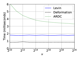
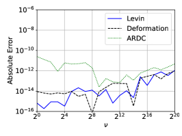
Figure 1: The results of the experiment of Subsection 5.1 in which the Levin-type method of this paper, the smooth deformation scheme of BremerPhase and the ARDC method of agocs are compared. The left-most plot gives the time required by each algorithm as a function of $\nu$, but only for the low-frequency regime. The middle plot gives the time required by each algorithm in the high-frequency regime. The plot on the right shows the absolute error in the value of the Legendre $P_{\nu}(0.999)$ obtained by each algorithm as a function of $\nu$.

Figure 1 presents the results of this experiment. We observe that the method of this paper achieves similar accuracy to that of BremerPhase , but is a bit slower. Although agocs claims that ARDC achieves a ten times speed improvement over the method of BremerPhase , we have not found this to be the case. At frequencies below $2^{9}$, the ARDC method is both noticeably slower and less accurate than both the other methods. For example, when $\nu=2^{8}$, the algorithm of this paper takes around 1.8 milliseconds and achieves 13 digits of accuracy, that of BremerPhase takes approximately 0.81 milliseconds and achieves 15 digits of accuracy while the ARDC method takes more than 30 milliseconds and obtains only 11 digits of accuracy. In particular, ARDC can be as much as 15 times slower than the method of this paper and 30 times slower than the algorithm of BremerPhase . At higher frequencies, ARDC achieves similar levels of accuracy to BremerPhase and the method of this paper, but it is more than a factor of two slower than the algorithm of this paper and more than a factor of three slower than the method of BremerPhase . The discrepancy between results reported in agocs and the results of this experiment appears to be attributable to the use of an unoptimized, highly inefficient implementation of BremerPhase in the experiments of agocs .

As explained in Section 2, in the low-frequency regime, the running times of all three methods increase with $\omega$. However, once a certain frequency threshold is reached, the running times decrease rapidly and then become essentially independent of frequency, or even continue to decrease slowly as functions of $\omega$. We note that, in our plots, this phenomenon is more apparent in the case of the ARDC method because of the much greater cost of that algorithm in the low-frequency regime.

5.2 Comparison with Magnus-type exponential integrators

In our second experiment, we compared the performance of our algorithm with that of four methods based on Magnus-type exponential integrators. We use MG4 to refer to the $4^{th}$ order Magnus exponential integrator given by (2.9) in Iserles103 ; MG6 denotes the $6^{th}$ order Magnus exponential integrator specified by (3.10) in Blanes1 ; we use CF4 to refer to $4^{th}$ order two exponential commutator-free quasi-Magnus exponential integrator listed in Table 2 of Blanes3 ; and CF6 is the first of the $6^{th}$ order five exponential commutator-free quasi-Magnus exponential integrators listed in Table 3 of Blanes3 .

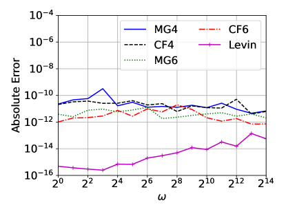
Figure 2: The errors in the solutions of the initial value problem of Subsection 5.2 obtained via four Magnus-type exponential integrator methods and the Levin-type algorithm of this paper.

The performance of exponential integrator methods depends critically on proper step length control. In order to give every possible benefit to the methods we compare our scheme against, we use the following two-phased approach. In the first phase, which was not timed, we determined a sequence of appropriate step sizes via a greedy algorithm. More explicitly, at each step, we started with a large step size $h$ and repeatedly reduced it by a factor of $0.95$ until an estimate of the local error fell bellow $\epsilon=10^{-12}$. The local error estimate was obtained by taking two steps of length $h/2$ in order to produce a (hopefully) superior approximation of the value of the solution at the terminal point. In the second phase, the equation was solved using the precomputed sequence of step lengths. It is only the second phase of the calculation which was timed.

For each $\omega=2^{0},2^{1},\ldots,2^{14}$ and each of the five methods, we solved the differential equation

$$y^{\prime\prime\prime}(t)+q_{2}(t)y^{\prime\prime}(t)+q_{1}(t)y^{\prime}(t)+q_{0}(t)y(t)=0,$$ (46)

where

$$q_{0}(t) =-\frac{\omega\left(e^{t}\omega-i\right)(\cos(8t)+3)\left(\left(t^{2}+1\right)\cos(3t)-i\omega\right)}{t^{2}+1}$$ (47)

$$q_{1}(t) =\frac{\omega\left(-\left(\omega+i\left(t^{2}+1\right)\right)\cos(8t)+e^{t}\omega\left(3t^{2}+\left(t^{2}+1\right)\cos(8t)+4\right)-3it^{2}-3\omega-4i\right)}{t^{2}+1}+$$

$$\ \ \ \ \cos(3t)\left(i\left(e^{t}-3\right)\omega-i\omega\cos(8t)+1\right)\ \ \ \mbox{and}$$

$$q_{2}(t) =i\left(\frac{1}{t^{2}+1}-e^{t}+3\right)\omega+i\omega\cos(8t)-\cos(3t)-1,$$

over the interval $[0,0.1]$ subject to the conditions

$$y(0)=1,\ \ \ y^{\prime}(0)=i\omega\ \ \ \mbox{and}\ \ \ y^{\prime\prime}(0)=(i\omega)^{2}.$$ (48)

The eigenvalues of the coefficient matrix corresponding to Equation (46) are

$$\lambda_{1}(t)=1+ie^{t}\omega,\ \ \ \lambda_{2}(t)=\cos(3t)-\frac{i\omega}{t^{2}+1}\ \ \ \mbox{and}\ \ \ \lambda_{3}(t)=-i\omega(\cos(8t)+3).$$ (49)

As in the case of the experiment of the last section, owing to the difficulty of computing solutions at arbitrary points using step methods, we assessed the accuracy of the obtained solutions by measuring the absolute error in their values at the endpoint $t=0.1$ of the solution domain only. Moreover, we only considered values of $\omega$ up to $2^{14}$ because the cost of finding appropriate step sizes becomes excessive for larger values of $\omega$.

$\omega$	MG4	CF4	MG6	CF6	Levin
$2^{0}$	2.79$\times 10^{-03}$	3.77$\times 10^{-03}$	9.70$\times 10^{-04}$	9.89$\times 10^{-04}$	6.88$\times 10^{-04}$
$2^{1}$	3.72$\times 10^{-03}$	4.96$\times 10^{-03}$	1.46$\times 10^{-03}$	1.46$\times 10^{-03}$	7.07$\times 10^{-04}$
$2^{2}$	7.42$\times 10^{-03}$	8.97$\times 10^{-03}$	2.95$\times 10^{-03}$	2.45$\times 10^{-03}$	7.35$\times 10^{-04}$
$2^{3}$	1.51$\times 10^{-02}$	1.47$\times 10^{-02}$	5.42$\times 10^{-03}$	3.44$\times 10^{-03}$	8.91$\times 10^{-04}$
$2^{4}$	2.55$\times 10^{-02}$	2.44$\times 10^{-02}$	9.71$\times 10^{-03}$	6.42$\times 10^{-03}$	7.57$\times 10^{-04}$
$2^{5}$	4.42$\times 10^{-02}$	4.59$\times 10^{-02}$	1.94$\times 10^{-02}$	1.23$\times 10^{-02}$	7.60$\times 10^{-04}$
$2^{6}$	7.79$\times 10^{-02}$	8.07$\times 10^{-02}$	3.48$\times 10^{-02}$	2.13$\times 10^{-02}$	7.61$\times 10^{-04}$
$2^{7}$	1.35$\times 10^{-01}$	1.40$\times 10^{-01}$	6.46$\times 10^{-02}$	3.99$\times 10^{-02}$	7.62$\times 10^{-04}$
$2^{8}$	2.48$\times 10^{-01}$	2.48$\times 10^{-01}$	1.13$\times 10^{-01}$	7.21$\times 10^{-02}$	7.63$\times 10^{-04}$
$2^{9}$	4.35$\times 10^{-01}$	4.40$\times 10^{-01}$	2.14$\times 10^{-01}$	1.31$\times 10^{-01}$	7.43$\times 10^{-04}$
$2^{10}$	7.61$\times 10^{-01}$	7.59$\times 10^{-01}$	3.95$\times 10^{-01}$	2.41$\times 10^{-01}$	7.42$\times 10^{-04}$
$2^{11}$	1.35$\times 10^{+00}$	1.30$\times 10^{+00}$	6.96$\times 10^{-01}$	4.27$\times 10^{-01}$	7.41$\times 10^{-04}$
$2^{12}$	2.25$\times 10^{+00}$	2.25$\times 10^{+00}$	1.29$\times 10^{+00}$	7.93$\times 10^{-01}$	7.42$\times 10^{-04}$
$2^{13}$	3.88$\times 10^{+00}$	3.95$\times 10^{+00}$	2.27$\times 10^{+00}$	1.41$\times 10^{+00}$	7.40$\times 10^{-04}$
$2^{14}$	6.78$\times 10^{+00}$	7.02$\times 10^{+00}$	4.36$\times 10^{+00}$	2.74$\times 10^{+00}$	7.41$\times 10^{-04}$

Table 1: The time, in second, required by four Magnus-type exponential integrator methods and the Levin-type algorithm of this paper to solve the initial value problem of Subsection 5.2.

Figure 2 and Table 1 give the results. We observe that all of the methods achieve reasonably accuracy given the requested level of precision. Not surprisingly, given the difference in the asymptotic behaviour of the running time of these algorithms with respect to frequency, the algorithm of this paper is orders of magnitude faster than the exponential integrator methods at high frequencies. In fact, when $\omega=2^{14}$, our approach is more than $3,000$ times faster than the most efficient of the exponential integrator methods. What is perhaps surprising, is that the algorithm of this paper is faster than the various exponential integrator methods even at very low frequencies. This is indicative of the fact that, even in the low-frequency regime, phase functions are not much more expensive to represent than the solutions of the scalar equation itself.

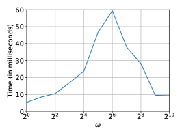
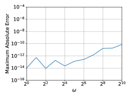
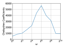
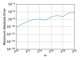
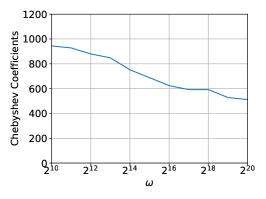
Figure 3: The results of the experiments of Subsection 5.3. The plot at top left gives the running time of the method of this paper in the low-frequency regime. The top-middle plot gives reports the absolute error in the solution of the boundary value problem for (50) in the low-frequency regime. The plot at top right shows the total number of piecewise Chebyshev coefficients required to represent the slowly-varying phase functions, again in the low-frequency regime. The plots on the bottom row provide the same information, but in the high-frequency regime.

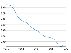
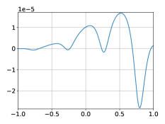
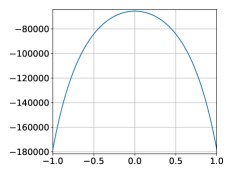
Figure 4: The derivatives of the three slowly-varying phase functions produced by applying the method of this paper to Equation (50) of Subsection 5.3 when the parameter $\omega$ is equal to $2^{16}$. Each column corresponds to one of the phase functions, with the real part appearing in the first row and the imaginary part in the second.

5.3 A boundary value problem for a third order equation

In the experiment described in this section, we considered the equation

$$y^{\prime\prime\prime}(t)+q_{2}(t)y^{\prime\prime}(t)+q_{1}(t)y^{\prime}(t)+q_{0}(t)y(t)=0,$$ (50)

where

$$q_{0}(t) =-ie^{t}t\omega\left(e^{t}-ie^{t^{2}}\omega\right)(\cos(12t)+2),$$ (51)

$$q_{1}(t) =e^{t^{2}}\omega\left(2\omega-ie^{t}t\right)+\omega\left(e^{t^{2}}\omega+ie^{t}(t+1)\right)\cos(12t)+e^{t}\left(e^{t}t+2i(t+1)\omega\right)\ \ \ \mbox{and}$$

$$q_{2}(t) =ie^{t^{2}}\omega-i\omega\cos(12t)-e^{t}(t+1)-2i\omega.$$

The eigenvalues of the coefficient matrix corresponding to (50) are

$$\lambda_{1}(t) =i\omega(\cos(12t)+2),\ \ \ \lambda_{2}(t) =te^{t}\ \ \ \mbox{and}\ \ \ \lambda_{3}(t) =e^{t}-ie^{t^{2}}\omega.$$ (52)

For each $\omega=2^{0},2^{1},\ldots,2^{20}$, we used our algorithm to solve (50) over the interval $[-1,1]$ subject to the conditions

$$y(-1)=y(1)=1\ \ \ \mbox{and}\ \ \ y^{\prime}(-1)=0.$$ (53)

We measured the absolute error in each resulting solution at 10,000 equispaced points in the interval $[-1,1]$ via comparison with a reference solution constructed using the solver of Appendix A. The results are given in Figure 3 while Figure 4 contains plots of the derivatives of the three slowly-varying phase functions produced by applying the method of this paper to Equation (50) when $\omega=2^{16}$. As expected, the running time of the method of this paper increases until a certain frequency threshold is passed, at which point it falls precipitously before becoming slowing decreasing. The maximum observed absolute error in the solution grows consistently with $\omega$, which is as expected considering that the condition number of the problem deteriorates with increasing frequency. For all values of $\omega$ greater than or equal to $2^{9}$, less than 10 milliseconds was required to solve the boundary value problem and fewer than 1,000 Chebyshev coefficients were needed to represent the phase functions. No more than 60 milliseconds and 6,000 coefficients were required in the worst case. The frequency $\Omega$ of the problems considered increased from approximately 3.9 when $\omega=1$ to roughly 4,100,531 when $\omega=2^{20}$.

5.4 An initial value problem for a fourth order equation

In this experiment, we considered the linear scalar ordinary differential equation

$$y^{\prime\prime\prime\prime}(t)+q_{3}(t)y^{\prime\prime\prime}(t)+q_{2}(t)y^{\prime\prime}(t)+q_{1}(t)y^{\prime}(t)+q_{0}(t)y(t)=0$$ (54)

whose coefficient matrix has eigenvalues

$$\lambda_{1}(t)=\frac{t}{2}+ie^{t^{2}}\omega,\ \ \ \lambda_{2}(t)=\frac{i\omega}{t^{2}+2}+e^{it},\ \ \ \lambda_{3}(t)=\cos(3t)\ \ \ \mbox{and}\ \ \ \lambda_{4}(t)=-i\left(t^{2}+1\right)\omega.$$ (55)

Formulas for the coefficients $q_{0}$, $q_{1}$, $q_{2}$ and $q_{3}$ are too unwieldy to reproduce here, but they can be easily calculated from (55) using a computer algebra system. For each $\omega=2^{0},2^{1},\ldots,2^{20}$, we used the algorithm of this paper to solve (54) over the interval $[-1,1]$ subject to the conditions

$$y(0)=1,\ \ \ y^{\prime}(0)=i\omega,\ \ \ y^{\prime\prime}(0)=(i\omega)^{2}\ \ \ \mbox{and}\ \ \ y^{\prime\prime\prime}(0)=(i\omega)^{3}.$$ (56)

We measured the absolute error in each resulting solution at 10,000 equispaced points in the interval $[-1,1]$ via comparison with a reference solution constructed using the solver of Appendix A. The results are given in Figure 5. We observe that for all $\omega$ greater than or equal to $2^{9}$, fewer than $8$ milliseconds was required to solve the problem and less than $250$ piecewise Chebyshev coefficients were required to represent the phase functions. In the worst case, when $\omega=2^{6}$, the solver took around 92 milliseconds and 3,200 piecewise Chebyshev coefficients were needed. The frequency $\Omega$ of the problems considered ranged from around 2.97 when $\omega=1$ to approximately $3,067,403$ when $\omega=2^{20}$.

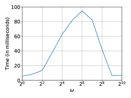
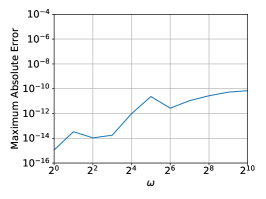
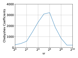
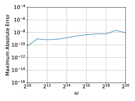
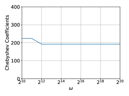
Figure 5: The results of the experiments of Subsection 5.4. The plot at top left gives the running time of the algorithm of this paper in the low-frequency regime. The top-middle plot gives reports the absolute error in the solution of the initial value problem for (54) in the low-frequency regime. The plot at top right shows the total number of piecewise Chebyshev coefficients required to represent the slowly-varying phase functions, again in the low-frequency regime. The plots on the bottom row provide the same information, but in the high-frequency regime.

6 Conclusions

We have described a numerical algorithm for the solution of linear scalar ordinary differential equations with slowly-varying coefficients whose running time is bounded independent of frequency. It is competitive with cutting edge methods for second order equations, and significantly faster than state-of-the-art methods for higher order equations. The key observation underlying our algorithm is that the solutions of scalar linear ordinary differential equations can be efficiently represented via phase functions. One of the main differences between our algorithm and many alternative approaches is that, rather than trying to approximate phase functions with a series expansion or an iterative process, we construct them by simply solving the Riccati equation numerically.

In the case of second order equations, the principles which underlie our solver have been rigorously justified. However, we have not yet proved the analogous results for higher order scalar equations. This is the subject of ongoing work by authors.

There are a number of obvious mechanisms for accelerating our algorithm. Perhaps the simplest would be to replace the robust but fairly slow solver of Appendix A with a faster method. We could also exploit the symmetries possessed by the solutions of the Riccati equation. For example, when the coefficient $q$ in the second order equation (9) is real-valued, there is a pair of slowly-varying phase functions $\psi_{1}$ and $\psi_{2}$ related by complex conjugation (i.e., $\psi_{1}=\overline{\psi_{2}}$) and it is only necessary to construct one of these phase functions.

The authors have also developed a “global” variant of the algorithm of this paper. Rather than applying the Levin procedure only to calculate the values of $r_{1},\ldots,r_{n}$ at a single point in the solution domain, it uses it as the basis of an adaptive method for calculating $r_{1},\ldots,r_{n}$ over the entire solution domain. This approach is generally faster than that of this paper in the event that all of the eigenvalues $\lambda_{1}(t),\ldots,\lambda_{n}(t)$ of the coefficient matrix for (2) are of large magnitude. However, when one or more of the eigenvalues is of small magnitude, the slowly-varying phase functions are nonunique and the method runs into difficulties. A preliminary discussion of the global variant of our algorithm can be found in aubry2023 ; a thorough description of it will be given by the authors at a later data. The authors also plan to describe the generalization of the algorithm of BremerPhase to equations of the form (1) and compare it to the method of this paper and its global variant.

It is straightforward to generalize our method to the case of scalar differential equations which are nondegenerate on an interval $[a,b]$ except at a finite collection of turning points. This can be done by applying the algorithm of this paper to a collection of subintervals of $[a,b]$.

Finally, we note that because essentially any system of linear ordinary differential equations can be transformed into a scalar equation (see, for instance, PutSinger ), the algorithm of this paper can be used to solve a large class of systems of linear ordinary differential equations in time bounded independent of frequency. The preprint hubremer introduces an algorithm based on this approach; that is, transforming a system of linear ordinary differential equations into a scalar equation which is then solved via the algorithm of this paper.

7 Acknowledgments

JB was supported in part by NSERC Discovery grant RGPIN-2021-02613. We thank Fruzsina Agocs for directing us to the version of the algorithm of agocs designed to solve Legendre’s equation used in the experiments of this paper.

8 Data availability statement

The datasets generated during and/or analysed during the current study are available from the corresponding author on reasonable request.

Appendix A An adaptive spectral solver for ordinary differential equations

In this appendix, we detail a standard adaptive spectral method for solving ordinary differential equations. It is used by the algorithm of this paper, and also to calculate reference solutions in our numerical experiments. We describe its operation in the case of the initial value problem

$$\left\{\begin{aligned} \bm{y}^{\prime}(t)&=F(t,\bm{y}(t)),\ \ \ a<t<b,\\ \bm{y}(a)&=\bm{v}\end{aligned}\right.$$ (57)

where $F:\mathbb{R}^{n+1}\to\mathbb{C}^{n}$ is smooth and $\bm{v}\in\mathbb{C}^{n}$. However, the solver can be easily modified to produce a solution with a specified value at any point $\eta$ in $[a,b]$. Moreover, by running the solver multiple times, a basis in the space of solutions of a system of differential equations can be constructed and used to solve boundary value problems as well.

The solver takes as input a positive integer $k$, a tolerance parameter $\epsilon$, an interval $(a,b)$, the vector $\bm{v}$ and a subroutine for evaluating the function $F$. It outputs $n$ piecewise $(k-1)^{st}$ order Chebyshev expansions, one for each of the components $y_{i}(t)$ of the solution $\bm{y}$ of (57).

The solver maintains two lists of subintervals of $(a,b)$: one consisting of what we term “accepted subintervals” and the other of subintervals which have yet to be processed. A subinterval is accepted if the solution is deemed to be adequately represented by a $(k-1)^{st}$ order Chebyshev expansion on that subinterval. Initially, the list of accepted subintervals is empty and the list of subintervals to process contains the single interval $(a,b)$. It then operates as follows until the list of subintervals to process is empty:

1. Find, in the list of subinterval to process, the interval $(c,d)$ such that $c$ is as small as possible and remove this subinterval from the list.

2. Solve the initial value problem

   $$\left\{\begin{aligned} \bm{u}^{\prime}(t)&=F(t,\bm{u}(t)),\ \ \ c<t<d,\\ \bm{u}(c)&=\bm{w}\end{aligned}\right.$$ (58)

   If $(c,d)=(a,b)$, then we take $\bm{w}=\bm{v}$. Otherwise, the value of the solution at the point $c$ has already been approximated, and we use that estimate for $\bm{w}$ in (58).

   If the problem is linear, a straightforward Chebyshev integral equation method is used to solve (58). Otherwise, the trapezoidal method is first used to produce an initial approximation $\bm{y_{0}}$ of the solution and then Newton’s method is applied to refine it. The linearized problems are solved using a Chebyshev integral equation method.

   In any event, the result is a set of $(k-1)^{st}$ order Chebyshev expansions

   $$u_{i}(t)\approx\sum_{j=0}^{k-1}\lambda_{ij}\ T_{j}\left(\frac{2}{d-c}t+\frac{c+d}{c-d}\right),\ \ \ i=1,\ldots,n,$$ (59)

   which purportedly approximate the components $u_{1},\ldots,u_{n}$ of the solution of (58).

3. Compute the quantities

   $$\frac{\sqrt{\sum_{j=k-2}^{k-1}\left|\lambda_{ij}\right|^{2}}}{\sqrt{\sum_{j=0}^{k-1}\left|\lambda_{ij}\right|^{2}}},\ \ \ i=1,\ldots,n,$$ (60)

   where the $\lambda_{ij}$ are the coefficients in the expansions (59). If any of the resulting values is larger than $\epsilon$, then we split the subinterval into two halves $\left(c,\frac{c+d}{2}\right)$ and $\left(\frac{c+d}{2},d\right)$ and place them on the list of subintervals to process. Otherwise, we place the subinterval $(c,d)$ on the list of accepted subintervals.

At the conclusion of this procedure, we have $(k-1)^{st}$ order piecewise Chebyshev expansions for each component of the solution, with the list of accepted subintervals determining the partition of $[a,b]$.

References

- (1) Agocs, F. J., and Barnett, A. H. An adaptive spectral method for oscillatory second-order linear ODEs with frequency-independent cost, arXiv:2212.06924, 2022.
- (2) Aubry, M., and Bremer, J. The Levin approach to the numerical calculation of phase functions, arXiv:2308.03288, 2023.
- (3) Aurentz, J., Mach, T., Robol, L., Vanderbril, R., and Watkins, D. S. Fast and backward stable computation of roots of polynomials, part II: Backward error analysis; companion matrix and companion pencil. SIAM Journal on Matrix Analysis and Applications 39 (2018), 1245–1269.
- (4) Aurentz, J., Mach, T., Vanderbril, R., and Watkins, D. S. Fast and backward stable computation of roots of polynomials. SIAM Journal on Matrix Analysis and Applications 36 (2015), 942–973.
- (5) Blanes, S., Casas, F., and Ros, J. Integrators based on the Magnus expansion. BIT Numerical Mathematics 40 (2000), 434–450.
- (6) Blanes, S., Casas, F., and Thalhammer, M. High-order commutator-free quasi-Magnus exponential integrators for non-autonomous linear evolution equations. Computer Physics Communications 220 (2017), 243–262.
- (7) Bremer, J. On the numerical calculation of the roots of special functions satisfying second order ordinary differential equations. SIAM Journal on Scientific Computing 39 (2017), A55–A82.
- (8) Bremer, J. On the numerical solution of second order differential equations in the high-frequency regime. Applied and Computational Harmonic Analysis 44 (2018), 312–349.
- (9) Bremer, J. Phase function methods for second order linear ordinary differential equations with turning points. Applied and Computational Harmonic Analysis 65 (2023), 137–169.
- (10) Chen, S., Serkh, K., and Bremer, J. The adaptive Levin method. arXiv 2209.14561 (2022).
- (11) Heitman, Z., Bremer, J., and Rokhlin, V. On the existence of nonoscillatory phase functions for second order ordinary differential equations in the high-frequency regime. Journal of Computational Physics 290 (2015), 1–27.
- (12) Hu, T., and Bremer, J. A frequency-independent solver for systems of first order linear ordinary differential equations, arXiv:2309.13848, 2023.
- (13) Iserles, A. On the global error of discretization methods for highly-oscillatory ordinary differential equations. BIT Numerical Mathematics 32 (2002), 561–599.
- (14) Iserles, A., Marthisen, A., and Nørsett, S. On the implementation of the method of Magnus series for linear differential equations. BIT Numerical Mathematics 39 (1999), 281–304.
- (15) Iserles, A., and Nørsett, S. P. On the solution of linear differential equations in Lie groups. Philosophical Transactions: Mathematical, Physical and Engineering Sciences 357, 1754 (1999), 983–1019.
- (16) Kummer, E. De generali quadam aequatione differentiali tertti ordinis. Progr. Evang. Köngil. Stadtgymnasium Liegnitz (1834).
- (17) Levin, D. Procedures for computing one- and two-dimensional integrals of functions with rapid irregular oscillations. Mathematics of Computation 38 (1982), 531–5538.
- (18) Li, J., Wang, X., and Wang, T. A universal solution to one-dimensional oscillatory integrals. Science in China Series F: Information Sciences 51 (2008), 1614–1622.
- (19) Li, J., Wang, X., Wang, T., and Xiao, S. An improved Levin quadrature method for highly oscillatory integrals. Applied Numerical Mathematics 60, 8 (2010), 833–842.
- (20) Magnus, W. On the exponential solution of differential equations for a linear operator. Communications on Pure and Applied Mathematics 7 (1954), 649–673.
- (21) Miller, P. D. Applied Asymptotic Analysis. American Mathematical Society, Providence, Rhode Island, 2006.
- (22) Put, M., and Singer, M. Galois Theory of Linear Differential Equations. Spinger Berlin, Heidelberg, 2003.
- (23) Spigler, R. Asymptotic-numerical approximations for highly oscillatory second-order differential equations by the phase function method. Journal of Mathematical Analysis and Applications 463 (2018), 318–344.
- (24) Spigler, R., and Vianello, M. A numerical method for evaluating the zeros of solutions of second-order linear differential equations. Mathematics of Computation 55 (1990), 591–612.
- (25) Spigler, R., and Vianello, M. The phase function method to solve second-order asymptotically polynomial differential equations. Numerische Mathematik 121 (2012), 565–586.
- (26) Wasow, W. Asymptotic expansions for ordinary differential equations. Dover, 1965.