Distances on the $\mathrm{CLE}_{4}$, critical Liouville quantum gravity and $3/2$-stable maps

Abstract

The purpose of this article is threefold. First, we show that when one explores a conformal loop ensemble of parameter $\kappa=4$ ($\mathrm{CLE}_{4}$) on an independent $2$-Liouville quantum gravity ($2$-LQG) disk, the surfaces which are cut out are independent quantum disks. To achieve this, we rely on approximations of the explorations of a $\mathrm{CLE}_{4}$: we first approximate the $\mathrm{SLE}_{4}^{\langle\mu\rangle}$ explorations for $\mu\in\mathbb{R}$ using explorations of the $\mathrm{CLE}_{\kappa}$ as $\kappa\uparrow 4$ and then we approximate the uniform exploration by letting $\mu\to\infty$. Second, we describe the relation between the so-called natural quantum distance and the conformally invariant distance to the boundary introduced by Werner and Wu. Third, we establish the scaling limit of the distances from the boundary to the large faces of $3/2$-stable maps and relate the limit to the $\mathrm{CLE}_{4}$-decorated $2$-LQG.

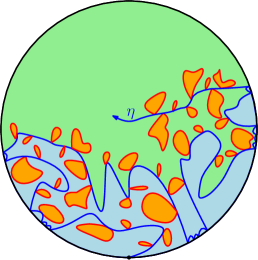
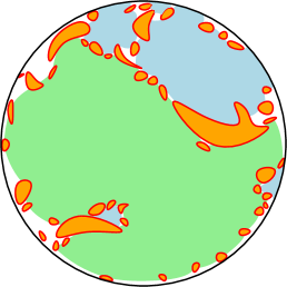
Figure 1: Left: illustration of the $\mathrm{SLE}^{\langle\mu\rangle}_{4}(-2)$ exploration of the $\mathrm{CLE}_{4}$ ensemble. Right: illustration of the uniform exploration of the $\mathrm{CLE}_{4}$ ensemble. The black curve $\eta$ is the trunk of the exploration. The unexplored region is in green, the domains encircled by loops are in orange and the cut out domains are in blue.

1 Introduction

1.1 Background

The conformal loop ensemble $\mathrm{CLE}_{4}$ is a random collection of disjoint simple loops included in some simply connected domain. It was introduced and studied in [She09] as part of the one parameter family of simple conformal loop ensembles $\mathrm{CLE}_{\kappa}$ for $\kappa\in(8/3,8)$, whose loops are no longer simple when $\kappa>4$. In [She09], Sheffield also defined a family of branching explorations parametrized by some “drift” $\mu$ of the $\mathrm{CLE}_{4}$ starting from the boundary and discovering the loops, called the $\mathrm{SLE}^{\langle\mu\rangle}_{4}(-2)$ exploration. According to [MSW17] this exploration can be described using a random simple continuous curve called the trunk of the exploration which hits the loops it discovers (see Figure 1). In [WW13], Werner and Wu introduced a uniform exploration of the $\mathrm{CLE}_{4}$ which can be seen as the limit of the $\mathrm{SLE}^{\langle\mu\rangle}_{4}(-2)$ exploration as $\mu\to\infty$. Informally, it consists in discovering the loop next to a random point chosen according to the harmonic measure on the boundary of the explored region and then updating this random point. The time parametrization of the uniform exploration in [WW13] is interpreted as a distance to the boundary. In an unpublished work [SWW], Sheffield, Watson and Wu argue that this distance from the boundary to the loops of the $\mathrm{CLE}_{4}$, which will be denoted by $\mathrm{d}_{\mathrm{WW}}$, can be extended to a conformally invariant distance between all the loops of the $\mathrm{CLE}_{4}$, including the boundary of the domain. However, we will not use this result in this work.

More recently, the $\mathrm{CLE}_{\kappa}$ was shown to interact nicely with an independent Liouville quantum gravity surface of parameter $\sqrt{\kappa}$ on the same simply connected domain ($\sqrt{\kappa}$-LQG). An LQG disk parametrized by a simply connnected domain can be defined as a well-chosen version of a Gaussian free-field on this domain which provides a way to measure quantum lengths of some curves and quantum area of sub-domains. In [MSW22], the law of the quantum boundary length of the unexplored region along the exploration of the $\mathrm{CLE}_{\kappa}$ for $\kappa<4$ parametrized by the quantum length of the trunk is shown to behave as some branching Markov process called a growth-fragmentation process, which was introduced by Bertoin in [Ber17]. For the case $\kappa=4$, building on the rich interplay between $\mathrm{CLE}$’s, LQG’s, and Brownian motion, and particularly on [DMS21], Aru, Holden, Powell and Sun identified in [AHPS23] a coupling between a uniform $\mathrm{CLE}_{4}$ exploration, an independent $2$-LQG disk and a Brownian excursion in the upper half-plane. Thanks to [AdS22], this coupling actually enables to describe the quantum boundary length of the explored region along the uniform exploration, parametrized by a so-called quantum natural distance to the boundary, as a growth-fragmentation process.

Independently, Boltzmann $3/2$-stable maps were first studied in [BCM18] in the infinite volume setting. In this introduction, we will only talk about finite $3/2$-stable maps. Recall that a planar map $\mathfrak{m}$ is a planar graph embedded in the sphere seen up to orientation preserving homeomorphism, with a distinguished oriented edge $\vec{e}_{r}$. The face on the right of the root edge is called the root face and is written $f_{r}$. We focus on bipartite planar maps, which only have faces with even degrees. For all $\ell\in\mathbb{N}$, let us denote by $\mathcal{M}^{(\ell)}$ the set of bipartite planar maps of perimeter $2\ell$, i.e. such that the degree of the root face is $2\ell$. Let ${\bf q}=(q_{k})_{k\geq 0}$ be a non-zero sequence of non-negative real numbers. The Boltzmann weight of a map $\mathfrak{m}\in\mathcal{M}^{(\ell)}$ is defined by

$$w_{\bf q}(\mathfrak{m})=\prod_{f\in\mathrm{Faces}(\mathfrak{m})\setminus\left\{f_{r}\right\}}q_{\deg(f)/2}.$$

When the partition function $W^{(\ell)}\coloneqq\sum_{\mathfrak{m}\in\mathcal{M}^{(\ell)}}w_{\bf q}(\mathfrak{m})$ is finite, we say that the weight sequence $\bf q$ is admissible. We further say that $\bf q$ is critical non-generic of type $2$ when

$$W^{(\ell)}\mathop{\sim}\limits_{\ell\to\infty}\frac{p_{\bf q}}{2}c_{\bf q}^{\ell+1}\ell^{-2}$$ (1.1)

for some constants $c_{\bf q},p_{\bf q}>0$. The Boltzmann probability measure on $\mathcal{M}^{(\ell)}$ is then defined by $\mathbb{P}^{(\ell)}(\mathfrak{m})=\frac{w_{\bf q}(\mathfrak{m})}{W^{(\ell)}}$ for all $\mathfrak{m}\in\mathcal{M}^{(\ell)}$. The associated mathematical expectation is written $\mathbb{E}^{(\ell)}$. A random variable of law $\mathbb{P}^{(\ell)}$ is called a $3/2$-stable map of perimeter $2\ell$. In what follows, ${\bf q}$ will be assumed critical non-generic of type $2$.

The distances that we will study on these maps are the graph distance on the dual map, obtained by exchanging the vertices with the faces, written $\mathrm{d}^{\dagger}_{\mathrm{gr}}$, and the first passage percolation distance, $\mathrm{d}^{\dagger}_{\mathrm{fpp}}$, which is obtained by putting i.i.d. parameter $1$ exponential random lengths on each edge of the dual map.

We studied the geometry of $3/2$-stable maps at the macroscopic scale in [Kam23] and proved that large $3/2$-stable planar maps do not satisfy scaling limits in the usual sense of Gromov-Hausdorff or Gromov-Prokhorov. The main technique in [BCM18] and [Kam23] to study these distances is the peeling exploration first introduced in [Bud16]. It consists in a step by step Markovian exploration of the map where at each step, we “peel” an edge on the boundary of the unexplored region and discover what is behind it. In this setting, we can also observe the evolution the perimeter of the unexplored region (which is the number of edges on its boundary).

1.2 Main results

Let us already state our main results more precisely even if the exact definitions will only arise in the next sections.

Exploration of $\mathrm{CLE}_{4}$ and LQG.

We choose to write the results for a particular branch of the exploration of the $\mathrm{CLE}_{4}$ on the unit disk $\mathbb{D}$ equipped with an independent $2$-LQG disk, namely the branch of the locally largest component: at each time the remaining to explore region splits in two regions, we choose to explore the region which has the largest quantum boundary length. We parametrize the uniform exploration by the so-called quantum natural distance to the boundary and the $\mathrm{SLE}^{\langle\mu\rangle}_{4}(-2)$ exploration by the quantum length of the trunk. These parametrizations are characterized as follows: if we denote by $(Y_{t})_{t\geq 0}$ (resp. $(Y^{\mu}_{t})_{t\geq 0}$) the càdlàg process of the quantum boundary length of the locally largest component along the uniform exploration (resp. $\mathrm{SLE}^{\langle\mu\rangle}_{4}(-2)$ exploration), then we have for all $t\geq 0$ the limit in probability

$$\lim_{\varepsilon\to 0}\varepsilon\#\{s\in[0,t],\ \lvert\Delta Y_{s}\rvert\in[\varepsilon,2\varepsilon]\}=\lim_{\varepsilon\to 0}\varepsilon\#\{s\in[0,t],\ \lvert\Delta Y^{\mu}_{s}\rvert\in[\varepsilon,2\varepsilon]\}=t,$$

where for any càdlàg process $(X_{t})_{t\geq 0}$ we write $\Delta X_{t}\coloneqq X_{t}-X_{t-}$ for all $t\geq 0$. The positive jumps of $(Y_{t})_{t\geq 0}$ or $(Y^{\mu}_{t})_{t\geq 0}$ occur when the exploration draws a loop while the negative jumps happen when a part of the unexplored region is cut out by the exploration.

Let us recall the positive self-similar Markov process studied in [AdS22], which corresponds to a particular case in a family of such processes introduced in [BBCK18] for $\theta=1$. Let $\Lambda_{1}$ be the image by $x\mapsto\log x$ of the measure ${1/(\pi(x(1-x))^{2})}{\bf 1}_{x\in(1/2,1)\cup(1,\infty)}dx.$ We denote by $\xi$ the Lévy process with no Brownian part, with drift $-2/\pi$ and Lévy measure $\Lambda_{1}$. If $\alpha\in\mathbb{R}$, we define the Lamperti time-substitution

$$\tau(t)=\inf\left\{r\geq 0\ ;\ \int_{0}^{r}e^{-\alpha\xi(s)}ds\geq t\right\}.$$ (1.2)

For all $x>0$, we write $P_{x}^{(\alpha)}$ the distribution of the time-changed process $X^{(\alpha)}(t)=xe^{\xi(\tau({tx^{\alpha}}))}$ with the convention that $X^{(\alpha)}(t)=\partial$ for $t\geq\zeta\coloneqq x^{-\alpha}\int_{0}^{\infty}e^{-\alpha\xi(s)}ds$. Then $X^{(\alpha)}$ is a self-similar Markov process of index $\alpha$, in the sense that for every $x>0$, the law of $(xX^{(\alpha)}(x^{\alpha}t))_{t\geq 0}$ under $P_{1}^{(\alpha)}$ is $P_{x}^{(\alpha)}$. By the definition of $\xi$, we can see that either $X^{(\alpha)}$ is absorbed a.s. at the cemetery point $\partial$ after a finite time, or it converges a.s. exponentially fast to zero. In the case $\alpha=-1$, we have $\zeta<+\infty$.

Our first main result is the analogue of Theorem 1.2 of [MSW22] in the case $\kappa=4$ for the $\mathrm{SLE}_{4}^{\langle\mu\rangle}(-2)$ exploration and for the uniform exploration.

Theorem 1.1.

Let $\mu\in\mathbb{R}$. The processes $(Y_{t})_{t\geq 0}$ and $(Y^{\mu}_{t})_{t\geq 0}$ have the same law as $(X^{(-1)}(\pi t))_{t\geq 0}$. Moreover, conditionally on $(Y_{s})_{0\leq s\leq t}$ (resp. $(Y^{\mu}_{s})_{0\leq s\leq t}$), if we denote by $(x_{i})_{i\geq 1}$ the sizes of the jumps of $(Y_{s})_{0\leq s\leq t}$ (resp. $(Y^{\mu}_{s})_{0\leq s\leq t}$) up to time $t$ ranked in the non-increasing order of absolute value, then the corresponding domains which are encircled by loops, associated with the positive jumps, or which are cut out, associated with the negative jumps, and the unexplored region are independent $2$-quantum disks of boundary lengths $|x_{i}|$’s and $Y_{t}$ (resp. $Y^{\mu}_{t}$).

Note that the fact that $(Y_{t})_{t\geq 0}$ has the same law as $(X^{(-1)}(\pi t))_{t\geq 0}$ can be seen as a direct consequence of Theorem 5.5 of [AHPS23] and Theorem 1.1 of [AdS22]. Besides, by focusing on the positive jumps, from the above theorem one recovers Theorem 1.1 of the recent article [AG23a].

Quantum natural distance and the conformally invariant distance.

For all $u\geq 0$, we denote by $C_{u}$ the unexplored region at time $u$ when following the locally largest component in the uniform exploration of [WW13] parametrized by the distance $\mathrm{d}_{\mathrm{WW}}$. We also denote by $\mathrm{d}_{\mathrm{q}}(\partial\mathbb{D},C_{u})$ the quantum natural distance from $C_{u}$ to the boundary $\partial\mathbb{D}$. Let $(\sigma(t))_{t\geq 0}$ be the right-continuous inverse of $u\mapsto\mathrm{d}_{\mathrm{q}}(\partial\mathbb{D},C_{u})$. The next result, a consequence of Theorem 1.1, gives some insight on $(\sigma(t))_{t\geq 0}$.

Theorem 1.2.

The process $(\sigma(t))_{t\geq 0}$ is continuous and increasing. Moreover, the continuous increasing process $S$ characterized by

$$\forall t\geq 0,\qquad\sigma(t)=S\left(\int_{0}^{t}\frac{1}{Y_{s}}ds\right)$$

has stationary increments.

However, we do not believe that $S$ has independent increments, see Subsection 7.2 for some heuristics. The above result motivates the introduction of another distance to the boundary: for every loop $\mathcal{L}$ which is discovered by the exploration of the locally largest component, we set $\mathrm{d}_{\mathrm{Lamperti}}(\partial\mathbb{D},\mathcal{L})\coloneqq\int_{0}^{\mathrm{d}_{\mathrm{q}}(\partial\mathbb{D},\mathcal{L})}{ds}/{Y_{s}}$. Then we have $\mathrm{d}_{\mathrm{WW}}(\partial\mathbb{D},\mathcal{L})=S(\mathrm{d}_{\mathrm{Lamperti}}(\partial\mathbb{D},\mathcal{L}))$.

$3/2$-stable maps and $\mathrm{CLE}_{4}$-decorated LQG.

Denote by $(P_{*}(n))_{n\geq 0}$ the perimeter process during the peeling exploration of the locally largest component (in terms of perimeter) under the law $\mathbb{P}^{(\ell)}$. Then it is known from Proposition 6.6 of [BBCK18] (which comes from Theorem 1 of [BCM18]) that under $\mathbb{P}^{(\ell)}$ the rescaled process $(P_{*}(\ell t)/\ell)_{t\geq 0}$ converges towards $(X^{(-1)}(\pi p_{\bf q}t))_{t\geq 0}$ where $p_{\bf q}$ is introduced in (1.1), so that by Theorem 1.1 the quantum length of the trunk of the $\mathrm{SLE}_{4}^{\langle\mu\rangle}(-2)$ exploration and the quantum natural distance corespond to the scaling limit of the time in the peeling exploration. The next results extend this relation between $3/2$-stable maps and $\mathrm{CLE}_{4}$-decorated LQG by establishing the scaling limit of the distances to the boundary.

By using some particular peeling algorithm, we can explore the map in a way that follows the growth of the balls centred at the root face $f_{r}$ or equivalently such that the distances from the edges on the boundary of the unexplored region to the root face are rouhly the same. For example, for $\mathrm{d}^{\dagger}_{\mathrm{gr}}$, the idea is to explore the map layer by layer: at first the edges at distance $0$ from the root face, then at distance $1$, etc. For $\mathrm{d}^{\dagger}_{\mathrm{fpp}}$, we use the uniform peeling exploration which takes at each step an edge uniformly at random in the boundary. See Subsection 6.1 for the definition of the peeling explorations. Let $\partial\overline{\mathfrak{e}}_{n}$ be the boundary of the explored region at time $n\geq 0$ using the appropriate peeling exploration for each distance. Then we prove that the radius of the balls during the exploration evolves in the following way:

$$\text{under }\mathbb{P}^{(\ell)},\qquad(\mathrm{d}^{\dagger}_{\mathrm{fpp}}(f_{r},\partial\overline{\mathfrak{e}}_{\lfloor\ell t\rfloor}))_{t\geq 0}\mathop{\longrightarrow}\limits_{\ell\to\infty}^{\mathrm{(d)}}\left(\int_{0}^{t}\frac{1}{2Y(p_{\bf q}s)}ds\right)_{t\geq 0};$$ (1.3)

$$\text{under }\mathbb{P}^{(\ell)},\qquad(\mathrm{d}^{\dagger}_{\mathrm{gr}}(f_{r},\partial\overline{\mathfrak{e}}_{\lfloor\ell t\rfloor})/(\log\ell))_{t\geq 0}\mathop{\longrightarrow}\limits_{\ell\to\infty}^{\mathrm{(d)}}\left(\int_{0}^{t}\frac{p_{\bf q}}{2Y(p_{\bf q}s)}ds\right)_{t\geq 0};$$ (1.4)

for the $J_{1}$ Skorokhod topology.

All our statements only focused so far on the locally largest component. But by the Markov property of Theorem 1.1 for the $\mathrm{CLE}_{4}$ exploration, and by the spatial Markov property of the peeling exploration, they can be extended to the convergence of the whole exploration tree. This enables us to state the scaling limit of the degree, the time of exploration and the distance to the boundary of large faces of $3/2$-stable maps towards the quantum boundary length, the quantum natural distance (or quantum length of the trunk depending on the exploration) and its Lamperti transform of a $\mathrm{CLE}_{4}$-decorated LQG disk.

Theorem 1.3.

For all $\ell\geq 1$, let $\mathfrak{M}^{(\ell)}$ of law $\mathbb{P}^{(\ell)}$. Let $(f_{i}^{(\ell)})_{i\geq 1}$ be the collection of faces of $\mathfrak{M}^{(\ell)}$ ranked in the non-increasing order of degree. Let $(n(f_{i}^{(\ell)}))_{i\geq 1}$ be the time at which they are discovered by the peeling by layers exploration. Let $(\mathcal{L}_{i})_{i\geq 1}$ be the collection of (outermost) loops of the $\mathrm{CLE}_{4}$ ranked in the non-increasing order of quantum boundary length. Let us denote by $\nu^{2}_{h^{2}}(\mathcal{L})$ the quantum boundary length of a loop $\mathcal{L}$, by $\mathrm{d}_{\mathrm{q}}(\partial\mathbb{D},\mathcal{L})$ the quantum natural distance to $\mathcal{L}$ and by $\mathrm{d}_{\mathrm{Lamperti}}(\partial\mathbb{D},\mathcal{L})$ its Lamperti transform defined by

$$\mathrm{d}_{\mathrm{Lamperti}}(\partial\mathbb{D},\mathcal{L})\coloneqq\int_{0}^{\mathrm{d}_{\mathrm{q}}(\partial\mathbb{D},\mathcal{L})}\frac{dt}{Y_{\mathcal{L}}(t)},$$

where $(Y_{\mathcal{L}}(t))_{0\leq t\leq\mathrm{d}_{\mathrm{q}}(\partial\mathbb{D},\mathcal{L})}$ is the quantum boundary length of the unexplored region surrounding $\mathcal{L}$ parametrized by the quantum natural distance. Then, for the product topology,

$$\left(\frac{\deg(f_{i}^{(\ell)})}{\ell},\frac{n(f_{i}^{(\ell)})}{p_{\bf q}\ell},\frac{2\mathrm{d}^{\dagger}_{\mathrm{gr}}(f_{r},f_{i}^{(\ell)})}{\log\ell}\right)_{i\geq 1}\mathop{\longrightarrow}\limits_{\ell\to\infty}^{(\mathrm{d})}\left(\nu^{2}_{h^{2}}(\mathcal{L}_{i}),\mathrm{d}_{\mathrm{q}}(\partial\mathbb{D},\mathcal{L}_{i}),\mathrm{d}_{\mathrm{Lamperti}}(\partial\mathbb{D},\mathcal{L}_{i})\right)_{i\geq 1}.$$

The same theorem can be stated for the $\mathrm{SLE}_{4}^{\langle\mu\rangle}(-2)$ exploration, replacing the quantum natural distance by the quantum length of the trunk. For the fpp distance, the factor $\log\ell$ is replaced by a factor $1/p_{\bf q}$ and the peeling by layers exploration is replaced by the uniform peeling exploration.

1.3 Outline

In Section 2 we recall the definition of the uniform exploration of the $\mathrm{CLE}_{4}$ from [WW13] and the definitions of $\gamma$-LQG disks for $\gamma\in(\sqrt{2},2]$ from [AHPS23]. The definition of the $\mathrm{SLE}^{\langle\mu\rangle}_{4}(-2)$ exploration is postponed to the next section.

Then, in Section 3, after introducing the remaining definitions, we prove Theorem 1.1 for the $\mathrm{SLE}^{\langle\mu\rangle}_{4}(-2)$ exploration by approximating the exploration with some well-chosen $\mathrm{SLE}_{\kappa}^{\beta}(\kappa-6)$ exploration, using the results of [Leh23] and by approximating the $2$-LQG disks with $\sqrt{\kappa}$-LQG disks relying on [AHPS23].

Next, in Section 4, so as to obtain the statement of Theorem 1.1 for the uniform exploration, we approximate the uniform exploration with the $\mathrm{SLE}^{\langle\mu\rangle}_{4}(-2)$ exploration as $\mu\to\infty$. This section relies partly on the same ideas as in Section 3.

On the basis of Theorem 1.1, using the Poissonian structure of the uniform exploration in [WW13], we prove Theorem 1.2 in Section 5.

In Section 6, we first establish the metric growth in the infinite volume setting using results of [BCM18]. By absolute continuity, we prove the convergences (1.3) and (1.4). We then describe the limit of the whole exploration tree and deduce Theorem 1.3. Our approximation results are informally summarized by the following diagram:

Finally in Section 7, we describe the applications to $O(2)$-loop decorated planar maps and we argue why the conformally invariant distance from [WW13] is not the Lamperti transform of the quantum natural distance.

2 Preliminaries on the uniform exploration of $\mathrm{CLE}_{4}$ and LQG

In this section, we first define the uniform exploration of the $\mathrm{CLE}_{4}$ and then we given some background on Liouville quantum gravity anf quantum disks.

2.1 The uniform exploration of the $\mathrm{CLE}_{4}$

We recall here the uniform exploration of the $\mathrm{CLE}_{4}$ introduced in [WW13]. Let $E$ be the space of positive excursions defined by

$$E=\{e\in\mathcal{C}(\mathbb{R}_{+},\mathbb{R}_{+});\ e(0)=0\text{ and }\tau(e)\coloneqq\sup\{s>0;\ e(s)>0\}\in(0,\infty)\}.$$

Let $\lambda$ be the Itô excursion measure on $E$, which is characterized by the fact that for any $x>0$, the measure of the subset $E_{x}$ of excursions of height at least $x$ is finite and if one renormalizes $\lambda$ so that it is a probabillity measure on $E_{x}$, then after reaching $x$ the excursion has the same law as a Brownian motion which is stopped when attaining zero. We denote by $\mathbb{H}$ the upper half-plane. If $e\in E$ is an excursion of duration $\tau(e)$, we define the driving function $w$ on $[0,\tau(e)]$ by

$$\forall t\in[0,\tau(e)],\qquad w_{t}=2e(t)-\int_{0}^{t}\frac{ds}{e(s)}.$$

It is shown in [SW12] that for $\lambda$-almost all $e\in E$, the conformal maps $g_{t}$ characterized by the ODE

$$g_{0}(z)=z\qquad\text{and}\qquad\forall s\geq t,\enskip\partial_{s}g_{s}(z)=\frac{2}{g_{s}(z)-w_{s}}$$

define a simple loop $\gamma=\gamma(e)$ in the upper half plane starting at zero, in the sense that the domain of definition of $g_{t}$ can be written $\mathbb{H}\setminus\gamma((0,t])$. We define the measure $\mu^{0}$ as the pushforward measure $\gamma_{*}\lambda$. For all $x\in\mathbb{R}$, we denote by $\mu^{x}$ the measure on loops rooted at $x$ obtained by translating $\mu^{0}$.

Let $z\in\mathbb{H}$. Let us first define the uniform exploration targeted at $z$. Let $(\hat{\gamma}_{u})_{u\geq 0}$ be a PPP of intensity $M=\int_{\mathbb{R}}dx\mu^{x}$. For every loop $\hat{\gamma}_{u}$, we denote by $\hat{f}_{u}$ the conformal transformation from the connected component of $\mathbb{H}\setminus\hat{\gamma}_{u}$ containing $z$ onto $\mathbb{H}$ which fixes the point $z$ and such that $\hat{f}_{u}^{\prime}(z)\in\mathbb{R}_{+}$. We define $\hat{F}^{z}_{u}=\hat{F}_{u}\coloneqq\circ_{0\leq v<u}\hat{f}_{v}$ where the composition is done in the order of appearance of the maps $\hat{f}_{u}$. This indeed defines a conformal map by p.19 of [WW13]. We also denote by $\tau^{z}$ the first time at which the loop $\hat{\gamma}_{u}$ surrounds the point $z$. We define $(\widetilde{\gamma}^{z}_{u})_{u\leq\tau^{z}}\coloneqq(\hat{F}_{u}^{-1}(\hat{\gamma}_{u}))_{u\leq\tau^{z}}$.

Lemma 8 from [WW13] shows that it is possible to couple two processes $(\widetilde{\gamma}^{z}_{u})_{u\leq\tau^{z}}$ and $(\widetilde{\gamma}^{z^{\prime}}_{u})_{u\leq\tau^{z^{\prime}}}$ so that they coincide until the time at which they disconnect $z$ from $z^{\prime}$. If we perform this coupling for a dense countable subset of $\mathbb{H}$ then the union of the loops surrounding points of this subset of $\mathbb{H}$ is the $\mathrm{CLE}_{4}$ ensemble. If we keep on drawing loops with $(\hat{F}_{u}^{-1}(\hat{\gamma}_{u}))_{u\geq 0}$ after the time $\tau^{z}$, we then build the nested $\mathrm{CLE}_{4}$ ensemble.

For future use, we come back to the unit disk $\mathbb{D}$ via a conformal transformation $\Phi:\mathbb{H}\rightarrow\mathbb{D}$ and we define the domain $D_{u}\subseteq\mathbb{D}$ of the unexplored points (during the uniform exploration of the non-nested $\mathrm{CLE}_{4}$) at time $u\geq 0$ by $D_{u}=\Phi(\left\{z\in\mathbb{H};\ \tau^{z}>u\right\})$. We also define for all $u\geq 0$ and $z\in\mathbb{D}$ the domain $\widetilde{D}^{z}_{u}\subseteq\mathbb{D}$ consisting in the unexplored points at time $u$ in the uniform exploration of the nested $\mathrm{CLE}_{4}$ targeted at $z$ by $\widetilde{D}^{z}_{u}=\Phi((F_{u}^{\Phi^{-1}(z)})^{-1}(\mathbb{H}))$. The choice of $\Phi$ does not change the law of the exploration by Proposition 9 of [WW13].

2.2 Critical Liouville quantum gravity and quantum disks

We recall here the definitions of the free boundary Gaussian free field (GFF) and of the $\gamma$-quantum disks for $\gamma\in(\sqrt{2},2]$ following [AHPS23]. See also [She07] for more details on GFF and [BP] for more about GFF and Liouville quantum gravity. We follow exactly the definitions in Subsection 4.1 of [AHPS23]. Let $D\subset\mathbb{C}$ be a simply connected domain with harmonically non-trivial boundary. We denote by $H(D)$ the Hilbert space closure of the space of real functions $f$ of class $\mathcal{C}^{\infty}$ on $D$ modulo constants which have finite Dirichlet energy (i.e. $\int_{D}\lvert\nabla f\rvert^{2}<\infty$), equipped with the Dirichlet inner product defined for any pair $f,g$ of such functions by

$$(f|g)_{\nabla}=\frac{1}{2\pi}\int_{D}\nabla f(z)\cdot\nabla g(z)d^{2}z,$$

where $d^{2}z$ is the Lebesgue measure on $\mathbb{C}$. Let $(f_{n})_{n\geq 0}$ be a Hilbert basis of $H(D)$. Let $(X_{n})_{n\geq 0}$ be i.i.d. random variables of law $\mathcal{N}(0,1)$. The free boundary GFF on $D$ is defined as the sum

$$h=\sum_{n\geq 0}X_{n}f_{n},$$

which converges in the space of distributions modulo constants. Even though the resulting random variable $h$ lives in the space of distributions modulo constants, one can fix that constant by assigning some particular value to $h$ on an arbitrary test function. The resulting random distribution is actually in the Sobolev space $H^{-1}_{\mathrm{loc}}(D)$ which is the space of distributions such that their restrictions to any relatively compact open domain $U\subset D$ are in the Sobolev space $H^{-1}(U)$. We endow the space $H^{-1}_{\mathrm{loc}}(D)$ with the corresponding limit topology which is metrizable and separable, such that a sequence converges in $H^{-1}_{\mathrm{loc}}(D)$ if and only if the restrictions to any relatively compact open domain $U$ converge in $H^{-1}(U)$.

Next, we recall that a $\gamma$-LQG surface for $\gamma\in(\sqrt{2},2]$ can be seen as an equivalence class of domains $D\subset\mathbb{C}$ equipped with a variant of the GFF $h$ (a free-boundary GFF plus a continuous random function on $\overline{D}$) under conformal maps. To that instance of the GFF, we associate an area and a boundary length measures $\mu^{\gamma}_{h}$ and $\nu^{\gamma}_{h}$. We define the area and boundary length measures $\mu^{\gamma}_{h}$ and $\nu^{\gamma}_{h}$ by the limits in probability: for $\gamma=2$, for all bounded open set $A\subseteq D$ we set

$$\mu^{2}_{h}(A)=\lim_{\delta\to 0}\int_{A}\left(-h_{\delta}+\log\left(\frac{1}{\delta}\right)\right)e^{2h_{\delta}(z)}\delta d^{2}z$$

and for all bounded open set $B\subseteq\partial D$

$$\nu^{2}_{h}(B)=\lim_{\delta\to 0}\int_{B}\left(-\frac{h_{\delta}}{2}+\log\left(\frac{1}{\delta}\right)\right)e^{h_{\delta}(z)}\delta dz,$$

while for $\gamma\in(\sqrt{2},2)$, for all bounded open set $A\subseteq D$, we set

$$\mu_{h}^{\gamma}(A)=\lim_{\delta\to 0}(8(2-\gamma))^{-1}\int_{A}\exp\left(\gamma h_{\delta}(z)\right)\delta^{\gamma^{2}/2}d^{2}z$$

and for all bounded open set $B\subseteq\partial D$

$$\nu_{h}^{\gamma}(B)=\lim_{\delta\to 0}(8(2-\gamma))^{-1}\int_{B}\exp\left(\frac{\gamma}{2}h_{\delta}(z)\right)\delta^{\gamma^{2}/4}dz,$$

where $d^{2}z$ is the Lebesgue measure on $\mathbb{C}$, $dz$ is the Lebesgue measure on $\mathbb{R}$ when $D$ is the upper half-plane $\mathbb{H}$ and $h_{\delta}(z)$ is the circular mean of $h$ on the circle of center $z$ and radius $\delta$.

We say that two pairs $(D,h)$ and $(\widetilde{D},\widetilde{h})$, where $D,\widetilde{D}$ are domains and $h,\widetilde{h}$ are distributions, are equivalent (as $\gamma$-quantum surfaces) if there exists a conformal map $\varphi:D\rightarrow\widetilde{D}$ such that

$$h=\widetilde{h}\circ\varphi+Q_{\gamma}\log|\varphi^{\prime}|\qquad\text{where}\qquad Q_{\gamma}=2/\gamma+\gamma/2.$$ (2.1)

If $h,\widetilde{h}$ are absolutely continuous with respect to a GFF plus a continuous function, then $\mu^{\gamma}_{\widetilde{h}}=\varphi_{*}\mu^{\gamma}_{h}$ and $\nu^{\gamma}_{\widetilde{h}}=\varphi_{*}\nu^{\gamma}_{h}$.

Informally, a $\gamma$-quantum disk (also called $\gamma$-LQG disk) corresponds to the domain encircled by a $\mathrm{CLE}_{\gamma^{2}}$ loop with the restriction of an infinite volume GFF. A quantum disk has a finite boundary length and a finite volume. More precisely, our unit-boundary length $\gamma$-quantum disks are defined as in Definition 4.1 for $\gamma=\sqrt{\kappa}\in(\sqrt{2},2)$ in [AHPS23] and Definition 4.3 for $\gamma=2$ from [AHPS23]. Let us summarize their definition although we will not rely on it since we will use directly the results of [AHPS23]. The definition is easier to state when we parametrize the disk by $\mathcal{S}\coloneqq\mathbb{R}\times(0,\pi)\subset\mathbb{C}$, the infinite strip. Let $h_{1}^{\gamma}$ be a function on $\mathcal{S}$ defined for all $s\in\mathbb{R}$ and $y\in(0,\pi)$ by $h_{1}^{\gamma}(s+iy)=\mathcal{B}^{\gamma}_{s}$, where $\mathcal{B}^{\gamma}$ is defined by:

1. For $\gamma\in(\sqrt{2},2)$, the function $(\mathcal{B}^{\gamma}_{s})_{s\geq 0}$ has the same law as $B_{2s}-Q_{\gamma}s$ conditioned to stay negative for all $s\geq 0$, where $(B_{s})_{s\geq 0}$ is a standard Brownian motion, while $(\mathcal{B}^{2}_{s})_{s\geq 0}$ is $(-\sqrt{2})$ times a Bessel process of dimension $3$ (which corresponds in some sense to $(B_{2s})_{s\geq 0}$ conditioned to stay negative by a famous result of Williams).

2. The process $(\mathcal{B}^{\gamma}_{-s})_{s\geq 0}$ is independent of $(\mathcal{B}^{\gamma}_{s})_{s\geq 0}$ and has the same law as $(\mathcal{B}^{\gamma}_{s})_{s\geq 0}$.

Let $h_{2}$ be the orthogonal projection of a free boundary GFF on $\mathcal{S}$ on the closure in $H(\mathcal{S})$ of the functions of mean zero along the vertical lines of $\mathcal{S}$. Set $h^{\gamma}_{s}=h_{1}^{\gamma}+h_{2}$ and let $\hat{h}^{\gamma}$ be a random distribution which has the law of $h^{\gamma}_{s}-(2/\gamma)\log\nu^{\gamma}_{h^{\gamma}_{s}}(\partial\mathcal{S})$ reweighted by $\nu^{\gamma}_{h^{\gamma}_{s}}(\partial\mathcal{S})^{(4/\gamma^{2})-1}$. Then the $\gamma$-quantum disk can be defined as the equivalence class of $(\mathcal{S},\hat{h}^{\gamma})$. We denote by $(\mathbb{D},h^{\gamma})$ the parametrization by the unit disk $\mathbb{D}$ of the unit boundary length $\gamma$-quantum disk.

One can define a marked quantum disk by sampling a marked boundary point according to the quantum boundary length measure, but we will not do this in this work. For $b>0$, we define the $b$-boundary length $\gamma$-quantum disk to be the quantum surface parametrized by $(\mathbb{D},h^{\gamma}+(2/\gamma)\log b)$. Note that $\nu^{\gamma}_{h^{\gamma}+(2/\gamma)\log b}=b\nu^{\gamma}_{h^{\gamma}}$ and $\mu^{\gamma}_{h^{\gamma}+(2/\gamma)\log b}=b^{2}\mu^{\gamma}_{h^{\gamma}}$.

2.3 The locally largest component and the quantum natural distance

Let $(\mathbb{D},h^{2})$ be a parametrization of a $2$-quantum disk by $\mathbb{D}$ and consider an independent uniform exploration of a $\mathrm{CLE}_{4}$ on $\mathbb{D}$. We want to focus on the quantum boundary length of the locally largest component of the exploration in terms of quantum boundary length. Informally, at each discovery of a loop, it goes on exploring the exterior of the loop and at each splitting event, it explores the domain which has the largest quantum boundary length. Let us first define formally this locally largest component. Let $(z_{j})_{j\geq 1}$ be an enumeration of $\mathbb{D}\cap\mathbb{Q}^{2}$. For all $j\geq 1$, for all $u\in[0,\tau^{z_{j}})$, let $D_{u}^{z_{j}}$ be the connected component of $D_{u}$ containing $z_{j}$. Using the restriction of $h^{2}$ to $D_{u}^{z_{j}}$, one can define the quantum boundary length

$$\mathcal{Y}^{z_{j}}_{u}\coloneqq\nu^{2}_{h^{2}_{|D_{u}^{z_{j}}}}(\partial D_{u}^{z_{j}})$$

of $D_{u}^{z_{j}}$ since it is encircled by $\mathrm{SLE}_{4}$-type curves.

Then, by the results of [AHPS23], the process $(\mathcal{Y}^{z_{j}}_{u})_{0\leq u<\tau^{z_{j}}}$ is a càdlàg process. Each positive jump corresponds to the discovery of a loop of the $\mathrm{CLE}_{4}$ and the size of the jump is exactly the quantum boundary length of the loop (computed using the restriction of $h^{2}$ to the domain encircled by the loop) while each negative jump at some time $u$ corresponds to the splitting of $D_{u-}^{z_{j}}$ into two components $D_{u}^{z_{j}}$ and $D_{u-}^{z_{j}}\setminus D_{u}^{z_{j}}$ and the size of the negative jump corresponds to the quantum boundary length of $D_{u-}^{z_{j}}\setminus D_{u}^{z_{j}}$.

The locally largest component $(C_{u})_{u\geq 0}$ is defined as follows. Let

$$\tau_{1}=\tau^{z_{1}}\wedge\inf\{u\geq 0;\ \mathcal{Y}^{z_{1}}_{u}<\mathcal{Y}^{z_{1}}_{u-}/2\}$$

be the first time $u$ at which $z_{1}$ is encircled by a loop or $\mathcal{Y}^{z_{1}}_{u}<\mathcal{Y}^{z_{1}}_{u-}/2$. For all $u<\tau_{1}$, we set $C_{u}=D^{z_{1}}_{u}$. We then define by induction a sequence $(\tau_{k})_{k\geq 1}$ and a subsequence $(z_{j_{k}})_{k\geq 1}$ by setting for all $k\geq 1$:

• If $\tau_{k}=\tau^{z_{j_{k}}}$, then $\tau_{k}$ is the time at which a loop $\mathcal{L}$ encircles $z_{j_{k}}$. Let $j_{k+1}$ be the first integer $j>j_{k}$ for which $z_{j}\in D_{\tau_{k}-}^{z_{j_{k}}}$ and such that $z_{j}$ is not encircled by $\mathcal{L}$.

• If $\tau_{k}=\inf\{u\geq 0;\ \mathcal{Y}^{z_{j_{k}}}_{u}<\mathcal{Y}^{z_{j_{k}}}_{u-}/2\}$, then $\tau_{k}$ is the first splitting time at which $z_{j_{k}}$ lies in the component with smallest quantum boundary length. Let $j_{k+1}$ be the first integer $j>j_{k}$ for which $z_{j}\in D_{\tau_{k}-}^{z_{j_{k}}}\setminus D_{\tau_{k}}^{z_{j_{k}}}$.

In both cases we set

$$\tau_{k+1}=\tau^{z_{j_{k+1}}}\wedge\inf\{u\geq 0;\ \mathcal{Y}^{z_{j_{k+1}}}_{u}<\mathcal{Y}^{z_{j_{k+1}}}_{u-}/2\}\qquad\text{and}\qquad\forall u\in[\tau_{k},\tau_{k+1}],\ C_{u}=D^{z_{j_{k+1}}}_{u}.$$

Let $z\in\bigcap_{k\geq 0}C_{\tau_{k}}$ (it exists since the intersection can be written as a decreasing intersection of compact sets). Notice that $z$ cannot be part of a loop otherwise it would not be in the $C_{\tau_{k}}$ for all $k\geq 0$. Then for all $k\geq 0$, for all $u\leq\tau_{k}$, we have $C_{u}=\widetilde{D}_{u}^{z}$ and as a result $\tau_{k}\to\infty$ as $k\to\infty$. Thus, $C_{u}$ is well-defined for all $u\geq 0$. Notice that by Lemma 8 of [WW13], the process $(C_{u})_{u\geq 0}$ does not depend on the choice of the enumeration $(z_{j})_{j\geq 1}$. For all $u\geq 0$, we set

$$\mathcal{Y}(u)\coloneqq\nu^{2}_{h^{2}_{|C_{u}}}(\partial C_{u}).$$

Following Equation (5.2) of [AHPS23] and Remark 2.3 of [MSW22], we define the quantum natural distance from $\partial\mathbb{D}$ to $C_{u}$ as the limit in probability

$$\mathrm{d}_{\mathrm{q}}(\partial\mathbb{D},C_{u})=\lim_{\varepsilon\to 0}\varepsilon\#\{s\in[0,u],\ \lvert\Delta\mathcal{Y}_{s}\rvert\in[\varepsilon,2\varepsilon]\}.$$ (2.2)

It is clear that $(\mathrm{d}_{\mathrm{q}}(\partial\mathbb{D},C_{u}))_{u\geq 0}$ is non-decreasing. Moreover, it is adapted with respect to the natural filtration of $\mathcal{Y}$. We denote by $\sigma$ the right-continuous inverse of $(\mathrm{d}_{\mathrm{q}}(\partial\mathbb{D},C_{u}))_{u\geq 0}$ and for all $t\geq 0$ we set $Y_{t}=\mathcal{Y}_{\sigma(t)}$.

3 The convergence $\kappa\uparrow 4$

In this section, we prove Theorem 1.1 for the $\mathrm{SLE}^{\langle\mu\rangle}_{4}(-2)$ exploration. To this end, we approximate the $\mathrm{SLE}_{\kappa}^{\langle\mu\rangle}$ explorations of the $\mathrm{CLE}_{4}$ decorated $2$-quantum disk by explorations of a $\mathrm{CLE}_{\kappa}$-decorated $\sqrt{\kappa}$-quantum disk as $\kappa\uparrow 4$, relying on the convergence results of [Leh23] and [AHPS23] so as to transfer the analogous property of [MSW22]. But first, we recall the definition on the Carathéodory topology and the $\mathrm{SLE}_{\kappa}^{\beta}(\kappa-6)$ and $\mathrm{SLE}_{4}^{\langle\mu\rangle}(-2)$ explorations.

3.1 Carathéodory topology

We first provide some useful results on Carathéodory topology. Let $z\in\mathbb{C}$. For all $n\geq 0$, let $U_{n}\subset\mathbb{C}$ be a simply connected domain. Let $U\subset\mathbb{C}$ be a simply connected domain containing $z$. When $z\in U_{n}$, let $f_{n}$ (resp. $f$) be the unique conformal map from $\mathbb{D}$ to $U_{n}$ (resp. $U$) such that $f_{n}(0)=z$ (resp. $f(0)=z$) and $f^{\prime}_{n}(0)>0$ (resp. $f^{\prime}(0)>0$). We recall that $U_{n}$ converges to $U$ as $n\to\infty$ in the Carathéodory topology if $z\in U_{n}$ for $n$ large enough and $f_{n}$ converges to $f$ uniformly on compact subsets of $\mathbb{D}$. Note that the convergence does not depend on the choice of $z\in U$ (see e.g. Lemma 2.2 of [BRY19]). The Carathéodory topology on the space of simply connected open domains of $\mathbb{C}$ containing $z$ is clearly metrizable. Still, with this definition, notice that a sequence $U_{n}$ which converges to $U$ in the sense of Carathéodory may also converge to another simply connected open domain $V$ such that $V\cap U=\emptyset$.

An equivalent definition of Carathéodory convergence (see for instance Definition 2.1 of [BRY19]), in fact the original one, states that $U_{n}$ converges to $U$ for the Carathéodory topology if and only if for every compact $K\subset U$, we have $K\subset U_{n}$ for all $n$ large enough and for every connected open set $V\ni z$, if $V\subset U_{n}$ for infinitely many $n$ then $V\subset U$. From this equivalent definition, it is not hard to see that the space of simply connected open domains of $\mathbb{C}$ containing $z$ is separable.

From this equivalent definition, one can see that for all compact $K\subset U$ the restriction of $f_{n}^{-1}$ to $K$ is well defined for $n$ large enough. Actually, as a consequence of Arzelà-Ascoli’s theorem, the convergence in the sense of Carathéodory of $U_{n}$ to $U$ implies the uniform convergence of $f_{n}^{-1}$ towards $f^{-1}$ on every compact subset of $U$. See Proposition 2.1 of [BRY19] for more details.

3.2 Background on $\mathrm{CLE}_{\kappa}$ explorations

We recall here the explorations of $\mathrm{CLE}_{\kappa}$ for $\kappa\in(8/3,4]$ defined in [She09]. We will not rely on the precise definition of the explorations and we refer to [She09] for details. If $\beta\in[-1,1]$, we define the skew Bessel process $(X_{u})_{u\geq 0}$ of dimension $\delta>0$ as the process such that $(|X_{u}|)_{u\geq 0}$ is a Bessel process of dimension $\delta$ and to each excursion of $(|X_{u}|)_{u\geq 0}$ we assign an independent sign: the corresponding excursion of $(X_{u})_{u\geq 0}$ is positive with probability $\frac{1+\beta}{2}$ and negative with probability $\frac{1-\beta}{2}$. When $\delta\neq 1$, we associate a process $(Y_{u})_{u\geq 0}$ to the skew Bessel process $X$ which is characterized by Proposition 3.8 of [She09]. In particular, it satisfies

$$\frac{dY_{u}}{du}=\frac{1}{X_{u}}\qquad\text{on}\qquad\left\{u\geq 0;\ X_{u}\neq 0\right\}.$$

In the case $\delta=1$, the process $(Y_{u})_{u\geq 0}$ is only defined when $\beta=0$ (and can be defined as the limit in law when $\delta\to 1$). Let $\mu\in\mathbb{R}$. One can obtain processes which satisfy the same properties as $(Y_{u})_{u\geq 0}$ in Proposition 3.8 of [She09] for $\delta=1$ by replacing $(Y_{u})_{u\geq 0}$ by $(Y_{u}-\mu\ell^{0}_{u})_{u\geq 0}$, where $(\ell^{0}_{u})_{u\geq 0}$ is the local time at zero of $(X_{u})_{u\geq 0}$. Let $\delta=3-8/\kappa$. If $\delta\neq 1$, then let $\beta\in[-1,1]$, otherwise let $\mu\in\mathbb{R}$. Let $(X_{u})_{u\geq 0}$ and $(Y_{u})_{u\geq 0}$ be the two processes defined above associated to $\delta,\beta$ when $\delta\neq 1$ and to $\delta,\mu$ when $\delta=1$. Let $(O_{u})_{u\geq 0}$ and $(W_{u})_{u\geq 0}$ be the processes given by $O_{0}=W_{0}=0$ and for all $u\geq 0$,

$$O_{u}=-\frac{2}{\sqrt{\kappa}}Y_{u}\qquad\text{and}\qquad W_{u}=O_{u}+\sqrt{\kappa}X_{u}.$$

Then the chordal $\mathrm{SLE}^{\beta}_{\kappa}(\kappa-6)$ for $\kappa\in(8/3,4)$ and the chordal $\mathrm{SLE}^{\left\langle\mu\right\rangle}_{4}(-2)$ from $0$ to $\infty$ in $\mathbb{H}$ are defined as the growing family of closed sets $(K_{u})_{u\geq 0}$ determined by the ODE

$$g_{0}(z)=z\qquad\text{and}\qquad\partial_{u}g_{u}(z)=\frac{2}{g_{u}(z)-W_{u}},$$

in the sense that the domain of definition of $g_{u}$ is $\mathbb{H}\setminus K_{u}$. In fact, it was shown in [MSW17] (in Theorem 7.4 for $\kappa\in(8/3,4)$ and in Proposition 5.3 for $\kappa=4$) that $\mathbb{H}\setminus K_{u}$ is the unbounded connected component of $\mathbb{H}\setminus\gamma([0,u])$ for some continuous path $\gamma$. On each excursion of $(X_{u})_{u\geq 0}$, the path $\gamma$ draws a simple loop. We also recall from Proposition 3.10 of [She09] that $(K_{u})_{u\geq 0}$ satisfies a “renewal property” stating that conditionally on $W_{u}$ up to a stopping time $T$ for which $O_{T}=W_{T}$ amost surely, the process $(W_{T+u}-W_{T})_{u\geq 0}$ has the same law as $(W_{u})_{u\geq 0}$, and a “conformal Markov property” stating that conditionally on $W_{u}$ up to some stoppping time $T$ for which a.s. $O_{T}\neq W_{T}$, the growing family given by the closure of $g_{T}(K_{T+u})$ up to the first time $u\geq 0$ such that $W_{T+u}=O_{T+u}$ has the same law (up to a time-change) as a chordal $\mathrm{SLE}_{\kappa}$ in $\mathbb{H}$ from $W_{T}$ to $O_{T}$. A chordal $\mathrm{SLE}^{\beta}_{\kappa}(\kappa-6)$ (or $\mathrm{SLE}^{\left\langle\mu\right\rangle}_{4}(-2)$ when $\kappa=4$) from $a$ to $b$ which are on the boundary of some simply connected domain $D\subset\mathbb{C}$ is just the image of the above $\mathrm{SLE}^{\beta}_{\kappa}(\kappa-6)$ (or $\mathrm{SLE}^{\left\langle\mu\right\rangle}_{4}(-2)$ when $\kappa=4$) by a conformal map sending $0$ to $a$ and $\infty$ to $b$. One can define the trunk $\eta$ of $\gamma$, a chordal $\mathrm{SLE}^{\beta}_{\kappa}(\kappa-6)$ (or $\mathrm{SLE}^{\left\langle\mu\right\rangle}_{4}(-2)$ when $\kappa=4$) as the path $\gamma$ where we removed the loops. In Theorem 7.4 of [MSW17], the trunk is shown to be an $\mathrm{SLE}_{\kappa^{\prime}}$-type curve for $\kappa^{\prime}=16/\kappa$. The path $\gamma$ can be decomposed into the trunk $\eta$ and the loops it traces along each excursion of $X$, see [MSW17] for details.

One can also define a radial version of the $\mathrm{SLE}^{\beta}_{\kappa}(\kappa-6)$ (or $\mathrm{SLE}^{\langle\mu\rangle}_{4}(-2)$ for $\kappa=4$) from $-i$ to $0$ in the unit disk $\mathbb{D}$, which is characterized by Proposition 3.13 of [She09] using the chordal $\mathrm{SLE}^{\beta}_{\kappa}(\kappa-6)$ (or $\mathrm{SLE}^{\langle\mu\rangle}_{4}(-2)$ for $\kappa=4$). As explained in [WW13, p. 11] one can define this radial version relying only on chordal $\mathrm{SLE}$’s as follows. Consider $\gamma_{1}$ a chordal $\mathrm{SLE}^{\beta}_{\kappa}(\kappa-6)$ (or $\mathrm{SLE}^{\langle\mu\rangle}_{4}(-2)$ for $\kappa=4$) from $-i$ to $i$, up to the first time $u_{1}$ at which it finishes to draw a loop intersecting the circle of radius $1/2$ centred at $-i$. Then, let $F_{1}$ be the conformal transformation from $D_{u_{1}}^{0}$ to $\mathbb{D}$ that keeps $0$ fixed and maps $\gamma_{1}(u_{1})$ to $-i$ and we repeat the same procedure again: growing $\gamma_{2}$ another independent chordal $\mathrm{SLE}^{\beta}_{\kappa}(\kappa-6)$ (or $\mathrm{SLE}^{\langle\mu\rangle}_{4}(-2)$ for $\kappa=4$) from $-i$ to $i$ until it draws a loop intersecting the circle of radius $1/2$ centred at $-i$, looking at its preimage by $F_{1}$ etc. The radial $\mathrm{SLE}^{\beta}_{\kappa}(\kappa-6)$ (or $\mathrm{SLE}^{\langle\mu\rangle}_{4}(-2)$ for $\kappa=4$) targeted at $z\in\mathbb{D}$ can be defined in a similar way.

By Proposition 3.14 of [She09], one can couple two radial $\mathrm{SLE}^{\beta}_{\kappa}(\kappa-6)$ (or $\mathrm{SLE}^{\left\langle\mu\right\rangle}_{4}(-2)$ when $\kappa=4$), $\gamma_{1}$ starting from $-i$ and targeted at $z_{1}\in\mathbb{D}$ and $\gamma_{2}$ from $-i$ to some $z_{2}\in\mathbb{D}$ so that they coincide up to some time-change until the time that $z_{1}$ and $z_{2}$ fail to lie in the same connected component of $\mathbb{H}\setminus\gamma_{1}([0,u])$. This property is called the target-invariance property. By performing this coupling with targets in a countable dense subset of $\mathbb{D}$, one can thus build the branching $\mathrm{SLE}^{\beta}_{\kappa}(\kappa-6)$ (or $\mathrm{SLE}^{\left\langle\mu\right\rangle}_{4}(-2)$ when $\kappa=4$) starting at $-i$ in $\mathbb{D}$, hence exploring all the loops of a $\mathrm{CLE}_{\kappa}$. It is also called the exploration tree. The radial and chordal $\mathrm{SLE}$’s can be seen as “branches” of this exploration tree.

3.3 Carathéodory convergence of the chordal exploration

We now describe an approximation result of the $\mathrm{SLE}^{\langle\mu\rangle}_{4}(-2)$ exploration in the sense of Carathéodory based on the results of [Leh23]. Let $\mu\in\mathbb{R}$. If $\kappa\in(8/3,4)$, let $(\gamma^{\kappa}(u))_{u\geq 0}$ be a chordal $\mathrm{SLE}^{\mu((4/\kappa)-1)}_{\kappa}(\kappa-6)$ in $\mathbb{D}$ from $-i$ to $i$. For all $u\geq 0$, if $X(u)=0$, then let $\upsilon^{\kappa}(u)=u$ and otherwise let $\upsilon^{\kappa}(u)$ be the time of the beginning of the excursion $X$ which is being drawn at time $u$. For all $u\geq 0$, for all $z\in\mathbb{D}\cap\mathbb{Q}^{2}$, let $D^{z,\kappa}_{u}$ be the connected component of $\mathbb{D}\setminus\gamma^{\kappa}([0,\upsilon^{\kappa}(u)])$ containing $z$. Let $(\gamma^{4}(u))_{u\geq 0}$ be a chordal $\mathrm{SLE}^{\langle\mu\rangle}_{4}(-2)$ in $\mathbb{D}$ from $-i$ to $i$. Let $\upsilon^{4}(u)$ for $u\geq 0$ be defined as before using the corresponding driving function. For all $u\geq 0$, for all $z\in\mathbb{D}$, let $D^{z,4}_{u}$ be the connected component of $\mathbb{D}\setminus\gamma^{4}([0,\upsilon^{4}(u)])$ containing $z$. Note that we choose to restrict the definition of the $D^{z,\kappa}_{u}$’s to the times $\upsilon^{\kappa}(u)$ since the relation with quantum disks that we will recall in the next subsection is only valid for these times. Then a consequence of the results of [Leh23] is the following proposition.

Proposition 3.1.

We have the convergence in law

$$\left(D^{z,\kappa}_{u}\right)_{u\geq 0,z\in\mathbb{Q}^{2}\cap\mathbb{D}}\enskip\mathop{\longrightarrow}\limits_{\kappa\uparrow 4}^{(\mathrm{d})}\enskip(D^{z,4}_{u})_{u\geq 0,z\in\mathbb{Q}^{2}\cap\mathbb{D}}$$ (3.1)

in terms of finite-dimensional distributions for the Carathéodory topology.

Proof.

We fix $\mu\in\mathbb{R}$. For all $\kappa\in(8/3,4]$, we denote by $(W^{\kappa}_{u})_{u\geq 0}$, $(O^{\kappa}_{u})_{u\geq 0}$, $(g^{\kappa}_{u})_{u\geq 0}$ and $(K^{\kappa}_{u})_{u\geq 0}$ the processes with which the $\mathrm{SLE}^{\mu((4/\kappa)-1)}_{\kappa}(\kappa-6)$ for $\kappa<4$ and $\mathrm{SLE}^{\langle\mu\rangle}_{4}(-2)$ for $\kappa=4$ is defined as described above. Let $\kappa_{n}$ be an increasing sequence tending to $4$. By Proposition 3.10 of [Leh23] we have the convergence of the driving functions:

$$(W^{\kappa_{n}},O^{\kappa_{n}})\mathop{\longrightarrow}\limits_{n\to\infty}^{(\mathrm{d})}(W^{4},O^{4})$$ (3.2)

for the topology of uniform convergence on compact sets. By Skorokhod’s representation theorem, we may suppose that the above convergence is almost sure. In particular, by Proposition 4.47 of [Law05], for all $u_{0}>0$, for all $\varepsilon>0$, we get a.s. the convergence

$$g^{\kappa_{n}}\mathop{\longrightarrow}\limits_{n\to\infty}g^{4}$$ (3.3)

uniformly on the set $[0,u_{0}]\times\left\{z\in\mathbb{H};\ d(z,K^{4}_{u_{0}})\geq\varepsilon\right\}$. In particular, we obtain the Carathéodory convergence of the unexplored region: for all $u\geq 0$,

$$\mathbb{H}\setminus K^{\kappa_{n}}_{u}\mathop{\longrightarrow}\limits_{n\to\infty}\mathbb{H}\setminus K^{4}_{u}\qquad\text{and}\qquad\mathbb{H}\setminus K^{\kappa_{n}}_{\upsilon^{\kappa_{n}}(u)}\mathop{\longrightarrow}\limits_{n\to\infty}\mathbb{H}\setminus K^{4}_{\upsilon^{4}(u)}.$$ (3.4)

We then look into the domains encircled by loops. Let $\varepsilon>0$. For all $i\geq 1$, for all $\kappa\in(8/3,4]$, let $e_{i,\varepsilon}^{\kappa}$ be the $i$-th excursion of $W^{\kappa}-O^{\kappa}$ of height larger than $\varepsilon$ and let $S_{i,\varepsilon}^{\kappa}<T_{i,\varepsilon}^{\kappa}$ be its starting time and end time. First notice that by (3.2) we get readily the uniform convergence of the excursions $e_{i,\varepsilon}^{\kappa_{n}}$’s to the $e_{i,\varepsilon}^{4}$’s and the convergence of their endpoints $S_{i,\varepsilon}^{\kappa_{n}},T_{i,\varepsilon}^{\kappa_{n}}$ to $S^{4}_{i,\varepsilon},T_{i,\varepsilon}^{4}$ as $n\to\infty$.

Let $u\in(S^{4}_{i,\varepsilon},T^{4}_{i,\varepsilon})$ and $\delta>0$. Applying Proposition 4.47 of [Law05] to $(W^{\kappa_{n}}_{(S^{\kappa_{n}}_{i,\varepsilon}+u)\wedge T^{\kappa_{n}}_{i,\varepsilon}})_{u\geq 0}$ which converges uniformly to $(W^{4}_{(S^{4}_{i,\varepsilon}+u)\wedge T^{4}_{i,\varepsilon}})_{u\geq 0}$ as $n\to\infty$, we know that for all $n$ large enough,

$$\left((v,z)\mapsto g^{\kappa_{n}}_{S^{\kappa_{n}}_{i,\varepsilon}+v}((g^{\kappa_{n}}_{S^{\kappa_{n}}_{i,\varepsilon}})^{-1}(z))\right)\mathop{\longrightarrow}\limits_{n\to\infty}\left((v,z)\mapsto g^{4}_{S^{4}_{i,\varepsilon}+v}((g^{4}_{S^{4}_{i,\varepsilon}})^{-1}(z))\right)$$ (3.5)

uniformly on $[0,u]\times\left\{z\in\mathbb{H};\ d(z,g^{4}_{S^{4}_{i,\varepsilon}}(K^{4}_{u}))\geq\delta\right\}$. In particular, for $n$ large enough,

$$\left\{z\in\mathbb{H};\ d(z,g^{4}_{S^{4}_{i,\varepsilon}}(K^{4}_{u}))\geq\delta\right\}\subset\mathbb{H}\setminus g^{\kappa_{n}}_{S^{\kappa_{n}}_{i,\varepsilon}}(K^{\kappa_{n}}_{u}).$$

In other words, for all $n$ large enough, the curve $(g^{\kappa_{n}}_{S^{\kappa_{n}}_{i,\varepsilon}}\circ\gamma^{\kappa_{n}})([S^{\kappa_{n}}_{i,\varepsilon},u])$ is included in the $\delta$-neighbourhood of $(g^{4}_{S^{4}_{i,\varepsilon}}\circ\gamma^{4})([S^{4}_{i,\varepsilon},u])$. Besides, let $U$ be the open ball centred at $g^{4}_{S^{4}_{i,\varepsilon}}(\gamma^{4}(u))$ of radius $\delta$. Then, by choosing $\delta$ small enough, $U$ is an open connected subset of $\mathbb{H}$ such that $U\cap(\mathbb{H}\setminus g^{4}_{S^{4}_{i,\varepsilon}}(K^{4}_{u}))\neq\emptyset$. By the Carathéodory convergence of $\mathbb{H}\setminus g^{\kappa_{n}}_{S^{\kappa_{n}}_{i,\varepsilon}}(K^{\kappa_{n}}_{u})$ towards $\mathbb{H}\setminus g^{4}_{S^{4}_{i,\varepsilon}}(K^{4}_{u})$ (which stems from (3.5)), we cannot have $U\subset\mathbb{H}\setminus g^{\kappa_{n}}_{S^{\kappa_{n}}_{i,\varepsilon}}(K^{\kappa_{n}}_{u})$ infinitely often, otherwise we would get that $\gamma^{4}(u)\in\mathbb{H}\setminus K^{4}_{u}$, which is not the case. Thus, for all $n$ large enough, $U\cap g^{\kappa_{n}}_{S^{\kappa_{n}}_{i,\varepsilon}}(K^{\kappa_{n}}_{u})\neq\emptyset$. By choosing $\delta$ small enough, by connectedness of $(g^{\kappa_{n}}_{S^{\kappa_{n}}_{i,\varepsilon}}\circ\gamma^{\kappa_{n}})([S^{\kappa_{n}}_{i,\varepsilon},u])$, we obtain that for $n$ large enough, $(g^{4}_{S^{4}_{i,\varepsilon}}\circ\gamma^{4})([S^{4}_{i,\varepsilon},u])$ is in the $\delta$-neighbourhood of $(g^{\kappa_{n}}_{S^{\kappa_{n}}_{i,\varepsilon}}\circ\gamma^{\kappa_{n}})([S^{\kappa_{n}}_{i,\varepsilon},u])$. We have thus proven that for all $u\in(S^{4}_{i,\varepsilon},T^{4}_{i,\varepsilon})$,

$$(g^{\kappa_{n}}_{S^{\kappa_{n}}_{i,\varepsilon}}\circ\gamma^{\kappa_{n}})([S^{\kappa_{n}}_{i,\varepsilon},u])\mathop{\longrightarrow}\limits_{n\to\infty}(g^{4}_{S^{4}_{i,\varepsilon}}\circ\gamma^{4})([S^{4}_{i,\varepsilon},u])$$ (3.6)

with respect to the Hausdorff distance.

For all $\kappa\in(8/3,4]$, let $R^{\kappa}_{i,\varepsilon}$ be the $i$-th time at which $W^{\kappa}-O^{\kappa}$ first reaches $\varepsilon$ after hitting zero. Then $R^{\kappa_{n}}_{i,\varepsilon}$ converges to $R^{4}_{i,\varepsilon}$ as $n\to\infty$. Moreover, for all $n\geq 0$, by the conformal Markov property the curve $g^{\kappa_{n}}_{R^{\kappa_{n}}_{i,\varepsilon}}\circ\gamma^{\kappa_{n}}_{|[R^{\kappa_{n}}_{i,\varepsilon},T^{\kappa_{n}}_{i,\varepsilon}]}$ has the same law as a chordal $\mathrm{SLE}(\kappa_{n})$ in $\mathbb{H}$ from $g^{\kappa_{n}}_{R^{\kappa_{n}}_{i,\varepsilon}}(\gamma^{\kappa_{n}}(R^{\kappa_{n}}_{i,\varepsilon}))=W^{\kappa_{n}}_{R^{\kappa_{n}}_{i,\varepsilon}}$ to $g^{\kappa_{n}}_{R^{\kappa_{n}}_{i,\varepsilon}}(\gamma^{\kappa_{n}}(T^{\kappa_{n}}_{i,\varepsilon}))=O^{\kappa_{n}}_{R^{\kappa_{n}}_{i,\varepsilon}}$. Furthermore, by taking Möbius transformations sending one of these two endpoints to $\infty$, and by applying Theorem 1.10 of [KS17] (which states that the chordal $\mathrm{SLE}(\kappa_{n})$ from $0$ to $\infty$ converges uniformly on compact sets to the $\mathrm{SLE}(4)$ as $n\to\infty$), we obtain the convergence

$$(g^{\kappa_{n}}_{R^{\kappa_{n}}_{i,\varepsilon}}\circ\gamma^{\kappa_{n}})([R^{\kappa_{n}}_{i,\varepsilon},T^{\kappa_{n}}_{i,\varepsilon}])\mathop{\longrightarrow}\limits_{n\to\infty}(g^{4}_{R^{4}_{i,\varepsilon}}\circ\gamma^{4})([R^{4}_{i,\varepsilon},T^{4}_{i,\varepsilon}])$$ (3.7)

for the Hausdorff distance. Besides, by $(\ref{eq cv g excursion})$ and by the convergence of $R^{\kappa_{n}}_{i,\varepsilon}$ to $R^{4}_{i,\varepsilon}$, we know that

$$g^{\kappa_{n}}_{R^{\kappa_{n}}_{i,\varepsilon}}\circ(g^{\kappa_{n}}_{S^{\kappa_{n}}_{i,\varepsilon}})^{-1}\mathop{\longrightarrow}\limits_{n\to\infty}g^{4}_{R^{4}_{i,\varepsilon}}\circ(g^{4}_{S^{4}_{i,\varepsilon}})^{-1}$$

uniformly on compact subsets of $\mathbb{H}\setminus(g^{4}_{S^{4}_{i,\varepsilon}}\circ\gamma^{4})([S^{4}_{i,\varepsilon},R^{4}_{i,\varepsilon}])$. Since the limiting function is a conformal map, it is easy to see that $g^{\kappa_{n}}_{S^{\kappa_{n}}_{i,\varepsilon}}\circ(g^{\kappa_{n}}_{R^{\kappa_{n}}_{i,\varepsilon}})^{-1}$ converges pointwise to $g^{4}_{S^{4}_{i,\varepsilon}}\circ(g^{4}_{R^{4}_{i,\varepsilon}})^{-1}$. By Montel’s theorem, we deduce that

$$g^{\kappa_{n}}_{S^{\kappa_{n}}_{i,\varepsilon}}\circ(g^{\kappa_{n}}_{R^{\kappa_{n}}_{i,\varepsilon}})^{-1}\mathop{\longrightarrow}\limits_{n\to\infty}g^{4}_{S^{4}_{i,\varepsilon}}\circ(g^{4}_{R^{4}_{i,\varepsilon}})^{-1}$$

uniformly on compact subsets of $\mathbb{H}$. Combining this with (3.7), we get that for all $\delta>0$ small enough,

$$(g^{\kappa_{n}}_{S^{\kappa_{n}}_{i,\varepsilon}}\circ\gamma^{\kappa_{n}})([R^{\kappa_{n}}_{i,\varepsilon},T^{\kappa_{n}}_{i,\varepsilon}])\cap V_{\delta}\mathop{\longrightarrow}\limits_{n\to\infty}(g^{4}_{S^{4}_{i,\varepsilon}}\circ\gamma^{4})([R^{4}_{i,\varepsilon},T^{4}_{i,\varepsilon}])\cap V_{\delta}$$ (3.8)

for the Hausdorff distance, where

$$V_{\delta}\coloneqq\left\{z\in\mathbb{H};\ d(z,g^{4}_{S^{4}_{i,\varepsilon}}(\gamma^{4}([S^{4}_{\varepsilon,i},R^{4}_{i,\varepsilon}]))\cup\mathbb{R})>\delta\right\}.$$

We are now in position to prove the Carathéodory convergence of the domain encircled by the loop. For all $n\in\mathbb{N}$, let $\mathcal{L}_{n}=g^{\kappa_{n}}_{S^{\kappa_{n}}_{i,\varepsilon}}(\gamma^{\kappa_{n}}([S^{\kappa_{n}}_{\varepsilon,i},T^{\kappa_{n}}_{\varepsilon,i}]))$ be the loop drawn by $u\mapsto W^{\kappa_{n}}_{(S^{\kappa_{n}}_{i,\varepsilon}+u)\wedge T^{\kappa_{n}}_{i,\varepsilon}}$ and let $\mathcal{L}=g^{4}_{S^{4}_{i,\varepsilon}}(\gamma^{4}([S^{4}_{\varepsilon,i},T^{4}_{\varepsilon,i}]))$ be the loop drawn by $u\mapsto W^{4}_{(S^{4}_{i,\varepsilon}+u)\wedge T^{4}_{i,\varepsilon}}$. By the convergence of $g^{\kappa_{n}}$ and $S_{i,\varepsilon}^{\kappa_{n}}$ as $n\to\infty$, to prove the Carathéodory convergence of the open domain encircled by the loop $\gamma^{\kappa_{n}}([S^{\kappa_{n}}_{\varepsilon,i},T^{\kappa_{n}}_{\varepsilon,i}])$ towards the domain encircled by $\gamma^{4}([S^{4}_{\varepsilon,i},T^{4}_{\varepsilon,i}])$, it suffices to prove the Carathéodory convergence of the domain $\mathcal{B}_{n}$ encircled by $\mathcal{L}_{n}$ towards the domain $\mathcal{B}$ encircled by $\mathcal{L}$.

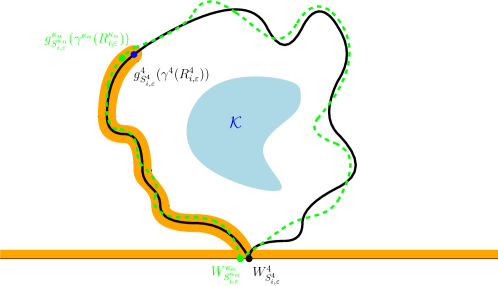
Figure 2: Illustration of the proof of the Carathéodory convergence of the domain encircled by $\mathcal{L}_{n}=g^{\kappa_{n}}_{S^{\kappa_{n}}_{i,\varepsilon}}(\gamma^{\kappa_{n}}([S^{\kappa_{n}}_{\varepsilon,i},T^{\kappa_{n}}_{\varepsilon,i}]))$, in green dashes, towards the domain encircled by $\mathcal{L}=g^{4}_{S^{4}_{i,\varepsilon}}(\gamma^{4}([S^{4}_{\varepsilon,i},T^{4}_{\varepsilon,i}]))$, in black. The complement of $V_{\delta}$ is in orange. A compact $\mathcal{K}$ encircled by $\mathcal{L}$ is drawn in blue.

Let $\mathcal{K}$ be a compact subset of the open domain $\mathcal{B}$. Then we may take $\delta>0$ small enough such that $\mathcal{K}\subset V_{\delta}$, so that by (3.8), we obtain that $\mathcal{K}\cap(g^{\kappa_{n}}_{S^{\kappa_{n}}_{i,\varepsilon}}\circ\gamma^{\kappa_{n}})([R^{\kappa_{n}}_{i,\varepsilon},T^{\kappa_{n}}_{i,\varepsilon}])=\emptyset$ for $n$ large enough. Moreover, by (3.6), we have that for $u>0$ small enough, for all $n$ large enough, we have $(g^{\kappa_{n}}_{S^{\kappa_{n}}_{i,\varepsilon}}\circ\gamma^{\kappa_{n}})([S^{\kappa_{n}}_{i,\varepsilon},R^{\kappa_{n}}_{i,\varepsilon}+u])\subset V_{\delta}$. Therefore, by the convergence of $R^{\kappa_{n}}_{i,\varepsilon}$ to $R^{4}_{i,\varepsilon}$ we deduce that for all $n$ large enough, $\mathcal{K}\cap\mathcal{L}_{n}=\emptyset$. One can actually see that $\mathcal{K}$ is encircled by $\mathcal{L}_{n}$ for $n$ large enough using that the endpoints of the path $(g^{\kappa_{n}}_{S^{\kappa_{n}}_{i,\varepsilon}}\circ\gamma^{\kappa_{n}})([R^{\kappa_{n}}_{i,\varepsilon},T^{\kappa_{n}}_{i,\varepsilon}])$ are in $\mathbb{H}\setminus V_{\delta}$ and applying (3.8) once more (see Figure 2).

Let $z\in\mathcal{B}$. To end the proof of the Carathéodory convergence of $\mathcal{B}_{n}$ towards $\mathcal{B}$, it suffices to show that if $U$ is a connected open set containing $z$ such that $U\subset\mathcal{B}_{n}$ infinitely often, then $U\subset\mathcal{B}$. Since $U$ and $\mathcal{B}$ are open it is enough to see that $U\subset\overline{\mathcal{B}}$. Assume by contradiction that there exists $w\in U\setminus\overline{\mathcal{B}}$. Take $\delta>0$ small enough so that $B(w,\delta)\subset U\setminus\overline{\mathcal{B}}$. In particular, $w\in V_{\delta}$. As a result, due to the Hausdorff convergences (3.6) and (3.8), the point $w$ is not encircled by $\mathcal{L}_{n}$ for $n$ large enough, hence a contradiction. We have thus proven that

$$\mathcal{B}_{n}\mathop{\longrightarrow}\limits_{n\to\infty}\mathcal{B}$$

in the sense of Carathéodory. This entails the convergence of the domains encircled by loops $\gamma^{\kappa_{n}}([S^{\kappa_{n}}_{\varepsilon,i},T^{\kappa_{n}}_{\varepsilon,i}])$ for $i\geq 1$ towards the domain encircled by $\gamma^{4}([S^{4}_{\varepsilon,i},T^{4}_{\varepsilon,i}])$. By letting $\varepsilon\to 0$, we get the Carathéodory convergence of all the domains encircled by loops.

Finally, we focus on the domains which are cut out by the exploration. Let $u\geq 0$. Let $x\in\mathbb{R}$. For all $n$, let $\zeta^{n}_{x}$ be the first time that $x$ is swallowed by $(g^{\kappa_{n}}_{u}({K}^{\kappa_{n}}_{v+u}))_{v\geq 0}$ and let $\zeta_{x}$ be the first time that $x$ is swallowed by $(g^{4}_{u}(K^{4}_{u+v}))_{v\geq 0}$. For all $n\geq 1$, let $C^{n}_{x}$ be the interior of $g^{\kappa_{n}}_{u}({K}^{\kappa_{n}}_{u+\zeta^{n}_{x}})\setminus g^{\kappa_{n}}_{u}({K}^{\kappa_{n}}_{u+\zeta^{n}_{x}-})$ and let $C_{x}$ be the interior of $g^{4}_{u}({K}^{4}_{u+\zeta_{x}})\setminus g^{4}_{u}({K}^{4}_{u+\zeta_{x}-})$. By the proof of Theorem 1.2 of [Leh23] and by another application of Skorokhod’s representation theorem, we know that $\zeta_{x}$ is the almost sure limit as $n\to\infty$ of $\zeta^{n}_{x}$. To be more precise, the proof of Theorem 1.2 of [Leh23] gives the convergence of $\zeta^{n}_{1}$, while the convergence of $\zeta^{n}_{x}$ follows by scale-invariance and reflexion-invariance. As a consequence, by considering chordal $\mathrm{SLE}_{\kappa_{n}}^{\mu((4/\kappa_{n})-1)}(\kappa_{n}-6)$’s and an $\mathrm{SLE}_{4}^{\langle\mu\rangle}(-2)$ targeted at $x$ and coupled with the chordal $\mathrm{SLE}_{\kappa_{n}}^{\mu((4/\kappa_{n})-1)}(\kappa_{n}-6)$’s and $\mathrm{SLE}_{4}^{\langle\mu\rangle}(-2)$ targeted at $\infty$ until $x$ is separated from $\infty$ and by applying the convergence (3.3), we obtain the a.s. convergence

$$C^{n}_{x}\mathop{\longrightarrow}\limits_{n\to\infty}C_{x}$$

as $n\to\infty$ in the sense of Carathéodory. By (3.4), we deduce the convergence of the cut out domain

$$(g_{u}^{\kappa_{n}})^{-1}(C^{n}_{x})\mathop{\longrightarrow}\limits_{n\to\infty}(g_{u}^{4})^{-1}(C_{x})$$

in the sense of Carathéodory. To conclude we just need to check that any cut out domain can be written in the form $(g_{u}^{4})^{-1}(C_{x})$ for some $u\geq 0$ and $x\in\mathbb{R}$. This is straightforward by taking $u\geq 0$ such that the frontier of the image by $g_{u}^{4}$ of the cut out domain has a non-trivial intersection with $\mathbb{R}$.

∎

3.4 The $\sqrt{\kappa}$-quantum disks and $\mathrm{CLE}_{\kappa}$

Here, we describe the results of [MSW22] that we want to transfer to $\kappa=4$. Recall Subsection 2.2. Let $\kappa\in(8/3,4]$. Let $(\mathbb{D},h^{\sqrt{\kappa}})$ be a parametrization of a unit boundary $\sqrt{\kappa}$-quantum disk. By Lemma 4.5 of [AHPS23], we know that

$$(h^{\sqrt{\kappa}},\mu_{h^{\sqrt{\kappa}}}^{\sqrt{\kappa}},\nu_{h^{\sqrt{\kappa}}}^{\sqrt{\kappa}})\mathop{\longrightarrow}\limits_{\kappa\uparrow 4}(h^{2},\mu^{2}_{h^{2}},\nu^{2}_{h^{2}}),$$ (3.9)

where the convergence of the first coordinate holds in the space $H^{-1}_{\mathrm{loc}}(\mathbb{D})$ while the convergences of the other coordinates hold with respect to the weak topology of measures. In what follows, when we speak of the convergence of some quantum disks, it always means the convergence of the GFF and of the quantum area and boundary length measures associated to the parametrization by the unit disk as in the above equation.

When we run an independent chordal $\mathrm{SLE}_{\kappa}^{\beta}(\kappa-6)$ (or $\mathrm{SLE}_{4}^{\langle\mu\rangle}(-2)$ for $\kappa=4$) $\gamma$ on a $\sqrt{\kappa}$-quantum disk $(\mathbb{D},h^{\sqrt{\kappa}})$, the trunk of $\gamma$ can be parametrized by its quantum length since it is an $\mathrm{SLE}_{\kappa^{\prime}}$-type process by Theorem 7.4 of [MSW17] and Remark 2.3 of [MSW22]. Notice that this quantum length is defined up to some multiplicative constant. Besides, we can define the quantum boundary length of $\mathrm{SLE}_{\kappa}$ type curves, such as the loops drawn by $\gamma$ or the boundary of the domains cut out by $\gamma$, via a quantum boundary length measure induced by $h^{\sqrt{\kappa}}$, using the quantum zipper properties first discovered in [She16]. The quantum boundary length measure on such a domain $D$ is equal to $\nu^{\sqrt{\kappa}}_{h^{\sqrt{\kappa}}_{|D}}$. We will see in the next proposition that they correspond exactly to the boundary length measures of some quantum disks.

We then state a result of [MSW22] for $\kappa\in(8/3,4)$, which gives the law of the quantum boundary length of the unexplored region and a Markov property in terms of quantum disks. Let $L_{0}$ (resp. $R_{0}$) be the quantum boundary length along the clockwise (resp. counterclockwise) segment from $-i$ to $i$ in $\partial\mathbb{D}$. Let $\beta\in(-1,1)$. Let $\gamma$ be a chordal $\mathrm{SLE}_{\kappa}^{\beta}(\kappa-6)$ from $-i$ to $i$ taken independently from the quantum disk $(\mathbb{D},h^{\sqrt{\kappa}})$. We parametrize its trunk $\eta$ by its quantum length. Let $T^{\kappa,\beta}$ be the total quantum length of the trunk. For each $t$ (corresponding here to the quantum length of the trunk), let $E_{t}$ be the event that the trunk has not yet attained $i$ before having quantum length $t$, i.e. $E_{t}=\{T^{\kappa,\beta}>t\}$. For all $t<T^{\kappa,\beta}$, we set $L^{\kappa,\beta}_{t}$ and $R^{\kappa,\beta}_{t}$ to be the left and right quantum boundary lengths of the unexplored region $\mathcal{D}^{\kappa}_{t}$ ($\mathcal{D}^{\kappa}_{t}$ is the connected component of $\mathbb{D}\setminus\gamma([0,\tau_{t}])$ containing $i$ in its closure, where $\tau_{t}$ is the time for $\gamma$ at which the quantum length of the trunk $\eta$ reaches $t$). More precisely, $L^{\kappa,\beta}_{t}$ is the quantum boundary length of the arc of $\partial\mathcal{D}^{\kappa}_{t}$ going from the tip of the trunk to $i$ in the clockwise direction and $R^{\kappa,\beta}_{t}$ is the quantum boundary length of the arc of $\partial\mathcal{D}^{\kappa}_{t}$ going from the tip of the trunk to $i$ in the anti-clockwise direction. Note that for all $t<T^{\kappa,\beta}$, we have $L^{\kappa,\beta}_{t}>0$ and $R^{\kappa,\beta}_{t}>0$. For all $t\geq T^{\kappa,\beta}$ we set $L^{\kappa,\beta}_{t}=R^{\kappa,\beta}_{t}=0$. If we write $S^{\kappa,\beta}_{t}=L^{\kappa,\beta}_{t}+R^{\kappa,\beta}_{t}$ for all $t\geq 0$, then $S^{\kappa,\beta}_{t}$ is the boundary length of $\mathcal{D}^{\kappa}_{t}$ for all $t<T^{\kappa,\beta}$. Let $a=1+4/\kappa$. Let $\widetilde{L}^{\beta,a}$ (resp. $\widetilde{R}^{\beta,a}$) be the $(a-1)$-stable Lévy process of Lévy measure $\Lambda_{L}^{\beta,a}\coloneqq\frac{1-\beta}{2}\cos(a\pi)(dx/x^{a}){\bf 1}_{x>0}+\frac{1}{2}(dx/|x|^{a}){\bf 1}_{x<0}$ (resp. $\Lambda_{R}^{\beta,a}\coloneqq\frac{1+\beta}{2}\cos(a\pi)(dx/x^{a}){\bf 1}_{x>0}+\frac{1}{2}(dx/|x|^{a}){\bf 1}_{x<0}$). The two processes $\widetilde{L}^{\beta,a}$ and $\widetilde{R}^{\beta,a}$ are taken independent. Let $\widetilde{S}^{a}=\widetilde{L}^{\beta,a}+\widetilde{R}^{\beta,a}$.

Proposition 3.2.

(Proposition 5.1 of [MSW22]) Up to some linear time-change, the process $(L^{\kappa,\beta}_{t},R^{\kappa,\beta}_{t})_{t\geq 0}$ is a Doob $h$-transform of the process $(\widetilde{L}^{\beta,a},\widetilde{R}^{\beta,a})$, in the sense that there exists a constant $c>0$ such that for all $t>0$, for all bounded measurable function $F:\mathbb{D}([0,t],\mathbb{R})^{2}\to\mathbb{R}$, for all $x,y>0$,

$$\mathbb{E} \left(\left.F\left((L^{\kappa,\beta}_{s},R^{\kappa,\beta}_{s})_{0\leq s\leq t}\right){\bf 1}_{E_{t}}\right|(L^{\kappa,\beta}_{0},R^{\kappa,\beta}_{0})=(x,y)\right)$$

$$=\mathbb{E}_{x,y}\left(\left(\frac{x+y}{\widetilde{S}^{a}_{ct}}\right)^{a}F\left((\widetilde{L}^{\beta,a}_{cs},\widetilde{R}^{\beta,a}_{cs})_{0\leq s\leq t}\right){\bf 1}_{\forall s\in[0,t],\ \widetilde{L}^{\beta,a}_{cs},\widetilde{R}^{\beta,a}_{cs}>0}\right),$$

where the Lévy process $\widetilde{L}^{\beta,a}$ (resp. $\widetilde{R}^{\beta,a}$) starts at $x$ (resp. $y$). Moreover, conditionally on the quantum boundary lengths $(L^{\kappa,\beta}_{s},R^{\kappa,\beta}_{s})_{0\leq s\leq t}$, the quantum surfaces which are cut out to the left, cut out to the right, inside the left loops or inside the right loops are independent $\sqrt{\kappa}$-quantum disks of quantum boundary lengths corresponding to the sizes of the positive and negative jumps of $L^{\kappa,\beta}$ and $R^{\kappa,\beta}$, while $(\mathcal{D}^{\kappa}_{t},h^{\sqrt{\kappa}}_{|\mathcal{D}_{t}})$ is an independent $\sqrt{\kappa}$-quantum disk of quantum boundary length $S^{\kappa,\beta}_{t}$.

When we parametrize the trunk by its quantum length, the parametrization is chosen up to a multiplicative constant, so that for our purpose we choose to take $c=1$ in the above proposition. This proposition will be a key ingredient to obtain analogous statements for $\kappa=4$.

3.5 Joint convergence of the $\mathrm{CLE}_{\kappa}$ and the $\sqrt{\kappa}$-quantum disks as $\kappa\uparrow 4$

In this subsection, we combine the convergences (3.1) and (3.9) to extend Proposition 3.2 to the case $\kappa=4$ for the chordal $\mathrm{SLE}_{4}^{\langle\mu\rangle}(-2)$. Then the statement of Theorem 1.1 for the $\mathrm{SLE}^{\langle\mu\rangle}_{4}(-2)$ exploration will be a direct corollary.

Let $(\mathbb{D},h^{2})$ be a unit boundary length $2$-quantum disk. Let $L_{0}^{4}$ (resp. $R_{0}^{4}$) be the quantum boundary length along the clockwise (resp. counterclockwise) segment from $-i$ to $i$ in $\partial\mathbb{D}$. Let $\mu\in\mathbb{R}$. Let $\gamma$ be an independent chordal $\mathrm{SLE}_{4}^{\mu}(-2)$ on $\mathbb{D}$ from $-i$ to $i$. We again parametrize the trunk by its quantum length and we denote by $T^{4,\mu}$ its total quantum length. For each $t\geq 0$ (corresponding here to the quantum length of the trunk), let $E_{t}$ be the event that the trunk has not yet attained $i$ before having quantum length $t$, i.e. $E_{t}=\{T^{4,\mu}>t\}$. For all $t<T^{4,\mu}$, we set $L_{t}^{4,\mu}$ and $R_{t}^{4,\mu}$ to be the left and right quantum boundary lengths of the remaining to be explored region $\mathcal{D}_{t}^{4}$ ($\mathcal{D}^{4}_{t}$ is the connected component of $\mathbb{D}\setminus\gamma([0,\tau_{t}])$ containing $i$ in its closure, where $\tau_{t}$ is the time for $\gamma$ at which the quantum length of the trunk reaches $t$). Note that for all $t<T^{4,\mu}$, we have $L_{t}^{4,\mu}>0$ and $R_{t}^{4,\mu}>0$. For all $t\geq T^{4,\mu}$, we set $L_{t}^{4,\mu}=R_{t}^{4,\mu}=0$. If we write $S^{4,\mu}_{t}=L^{4,\mu}_{t}+R^{4,\mu}_{t}$ for all $t\geq 0$, then $S^{4,\mu}_{t}$ is the quantum boundary length of $\mathcal{D}^{4}_{t}$ when $t<T^{4,\mu}$. Let $\widetilde{L}^{2}$ and $\widetilde{R}^{2}$ be two independent symmetric Cauchy processes of Lévy measure $\frac{1}{2}(dx/x^{2}){\bf 1}_{x\neq 0}$. Let $\widetilde{S}^{2}=\widetilde{L}^{2}+\widetilde{R}^{2}$.

Proposition 3.3.

The process $(S^{4,\mu}_{t})_{t\geq 0}$ satisfies the following absolute continuity relation: there exists a constant $c>0$ such that for all $t>0$, for all bounded measurable function $F:\mathbb{D}([0,t],\mathbb{R})^{2}\to\mathbb{R}$, for all $x,y>0$,

$$\mathbb{E}\left(\left.F\left((S^{4,\mu}_{s})_{0\leq s\leq t}\right){\bf 1}_{E_{t}}\right|(L^{4}_{0},R^{4}_{0})=(x,y)\right)=\mathbb{E}_{x,y}\left(\left(\frac{x+y}{\widetilde{S}^{2}_{ct}}\right)^{2}F\left((\widetilde{S}^{2}_{cs})_{0\leq s\leq t}\right){\bf 1}_{\forall s\in[0,t],\ \widetilde{L}^{2}_{cs},\widetilde{R}^{2}_{cs}>0}\right),$$ (3.10)

where the Cauchy process $\widetilde{L}^{2}$ (resp. $\widetilde{R}^{2}$) starts at $x$ (resp. $y$). Moreover, conditionally on $(S^{4,\mu}_{s})_{0\leq s\leq t}$, the quantum surfaces which are cut out or inside discovered loops before time $t$ are independent quantum disks of quantum boundary length corresponding to the sizes of the jumps of $(S^{4,\mu}_{s})_{0\leq s\leq t}$, while $(\mathcal{D}^{4}_{t},h^{2}_{|\mathcal{D}^{4}_{t}})$ is an independent quantum disk of quantum boundary length $S^{4,\mu}_{t}$.

Here we also choose the multiplicative constant for the quantum length of the trunk so that $c=1$ to be consistent with our choice of $c$ for Proposition 3.2. Note that the quantum length of the trunk of the chordal $\mathrm{SLE}_{4}^{\langle\mu\rangle}(-2)$ can also be defined using the quantum boundary length measure since it is an $\mathrm{SLE}_{4}$-type curve, so that there should be a choice for $c$ such that the quantum length of the trunk and the quantum boundary lengths of the cut out and encircled domains are defined using the same multiplicative constant. However, our approach does not enable us to identify this constant.

Remark 3.4.

The above proposition is not exatly the proper counterpart of Proposition 3.2 insofar as we do not describe the left and right quantum boundary lengths of the unexplored region, but only the whole quantum boundary length. To get the evolution of the left and right quantum boundary lengths, one has to identify the quantum surfaces which are cut out or encircled by a loop on the right side and on the left side of the trunk. For the cut out domains one can see from Proposition 3.1 that the domains which are cut out on the right (resp. left) side of the trunk are limits of domains which are cut out on the right (resp. left) side of the trunk. For the loops, one has to look at the direction the trunk takes after hitting the loops, using the proof of Proposition 3.1 once more. We do not go further in that direction since it is not the main purpose of this work.

Using Proposition 3.3, one can deduce Theorem 1.1 for the $\mathrm{SLE}_{4}^{\langle\mu\rangle}(-2)$ exploration:

Proof of Theorem 1.1 for $(Y^{\mu}_{t})_{t\geq 0}$ using Proposition 3.3.

Using the $\mathrm{SLE}_{4}^{\langle\mu\rangle}(-2)$ exploration tree, one can define the branch which follows the locally largest component in terms of quantum boundary length. It can be defined through an approximation as in Subsection 5.3 of [MSW22]: let $\varepsilon>0$, for each time of the form $\varepsilon n$ for $n\in\mathbb{N}$, one updates the target point for the chordal exploration and chooses the point such that the quantum boundary lengths on both sides of the unexplored region are equal. When $\varepsilon\to 0$, this exploration approximates the branch of the locally largest component. Denote by $(Y^{\mu}_{t})_{t\geq 0}$ the quantum boundary length of the locally largest component parametrized by the quantum length of the trunk (which is given by a concatenation of parts of trunks of chordal $\mathrm{SLE}_{4}^{\langle\mu\rangle}(-2)$’s). Then, using exactly the same reasoning as in Subsection 5.3 of [MSW22], we deduce from Proposition 3.3 the analogous result for the branch of the locally largest component, which is no more than the statement of Theorem 1.1 for $(Y^{\mu}_{t})_{t\geq 0}$. ∎

All this subsection is then devoted to the proof of Proposition 3.3. Let $(\mathbb{D},h^{\sqrt{\kappa}})$ be a parametrization of a unit-boundary $\sqrt{\kappa}$-quantum disk. We run an independent chordal $\mathrm{SLE}^{\mu((4/\kappa)-1)}_{\kappa}(\kappa-6)$ in $\mathbb{D}$ from $-i$ to $i$. We will prove the above result by letting $\kappa\uparrow 4$. The first step towards the above proposition is the convergence in law of the processes involved in Proposition 3.2. Let $(\overline{L}^{4}_{0},\overline{R}^{4}_{0})=(L^{4}_{0},R^{4}_{0})$ (see the beginning of Subsection 3.5). Next, conditionnally on $(\overline{L}^{4}_{0},\overline{R}^{4}_{0})=(x,y)$, define a process $(\overline{L}_{t}^{4},\overline{R}_{t}^{4})_{t\geq 0}$ via the same Doob $h$-transform as in Proposition 3.2 for $\kappa=4$, $a=1+4/\kappa=2$ and $\beta=0$, replacing $E_{t}$ by $\{\overline{L}_{t}^{4},\overline{R}_{t}^{4}>0\}$ and setting $\overline{L}_{t}^{4}=\overline{R}_{t}^{4}=0$ on the complement.

Lemma 3.5.

We have the convergence

$$(L_{t}^{\kappa,\mu((4/\kappa)-1)},R_{t}^{\kappa,\mu((4/\kappa)-1)})_{t\geq 0}\mathop{\longrightarrow}\limits_{\kappa\uparrow 4}^{(\mathrm{d})}(\overline{L}_{t}^{4},\overline{R}_{t}^{4})_{t\geq 0}$$ (3.11)

in the sense of Skorokhod.

Proof.

The convergence of $(L_{0}^{\kappa,\mu((4/\kappa)-1},R^{\kappa,\mu((4/\kappa)-1}_{0})$ stems from the convergence of the quantum boundary length measure in (3.9). Besides, one can see easily see that for all continuous bounded function $\varphi:\mathbb{R}\rightarrow\mathbb{R}$ vanishing on a neighbourhood of zero, we have

$$\int_{\mathbb{R}}\varphi(x)\Lambda_{L}^{\mu((4/\kappa)-1),(4/\kappa)+1}(dx)\mathop{\longrightarrow}\limits_{\kappa\uparrow 4}\int_{\mathbb{R}}\varphi(x)\frac{dx}{2x^{2}}$$

and

$$\int_{\mathbb{R}}\varphi(x)\Lambda_{R}^{\mu((4/\kappa)-1),(4/\kappa)+1}(dx)\mathop{\longrightarrow}\limits_{\kappa\uparrow 4}\int_{\mathbb{R}}\varphi(x)\frac{dx}{2x^{2}}.$$

It is classical (see e.g. [JS87] VII.3.6) that this implies the convergence of Lévy processes

$$\left(\widetilde{L}^{\mu((4/\kappa)-1),(4/\kappa)+1}_{t}\right)_{t\geq 0}\mathop{\longrightarrow}\limits_{\kappa\uparrow 4}^{(\mathrm{d})}\left(\widetilde{L}^{2}_{t}\right)_{t\geq 0}\enskip\text{and}\enskip\left(\widetilde{R}^{\mu((4/\kappa)-1),(4/\kappa)+1}_{t}\right)_{t\geq 0}\mathop{\longrightarrow}\limits_{\kappa\uparrow 4}^{(\mathrm{d})}\left(\widetilde{R}^{2}_{t}\right)_{t\geq 0},$$

for the $J_{1}$ Skorokhod topology. We then reason by absolute continuity. Let $t,\varepsilon>0$. By Proposition 3.2, if $F$ is a bounded continuous function on $\mathbb{D}([0,t],\mathbb{R})^{2}$ vanishing on $\{(f,g);\ \exists s\in[0,t],f(s)<\varepsilon\text{ or }g(s)<\varepsilon\}$, we have

$$\mathbb{E} \left(\left.F\left((L^{\kappa,\beta}_{s},R^{\kappa,\beta}_{s})_{0\leq s\leq t}\right){\bf 1}_{E_{t}}\right|(L^{\kappa,\beta}_{0},R^{\kappa,\beta}_{0})=(x,y)\right)$$

$$=\mathbb{E}_{x,y}\left(\left(\frac{x+y}{\widetilde{S}^{a}_{ct}}\right)^{a}F\left((\widetilde{L}_{cs}^{\beta,a},\widetilde{R}^{\beta,a}_{cs})_{0\leq s\leq t}\right){\bf 1}_{\forall s\in[0,t],\ \widetilde{L}^{\beta,a}_{cs},\widetilde{R}^{\beta,a}_{cs}>0}\right),$$

where we have set $\beta=\mu((4/\kappa)-1)$ and $a=(4/\kappa)+1$. One concludes by dominated convergence. ∎

Another ingredient is the fact that the convergences (3.1) and (3.9) imply the convergence of the underlying fields and quantum area measure of the cut out, encircled and unexplored surfaces:

Lemma 3.6.

If for all $z\in\mathbb{D}\cap\mathbb{Q}^{2}$, the function $f^{z,\kappa}_{u}$ is the unique conformal map from $\mathbb{D}$ to $D^{z,\kappa}_{u}$ which sends $0$ to $z$ such that $(f^{z,\kappa}_{u})^{\prime}(0)>0$, then jointly with (3.1) and (3.9),

$$\!\!\!\begin{pmatrix}f^{z,\kappa}_{u}\\ h^{\sqrt{\kappa}}\circ f^{z,\kappa}_{u}+Q_{\sqrt{\kappa}}\log|(f^{z,\kappa}_{u})^{\prime}|\\ \mu^{\sqrt{\kappa}}_{h^{\sqrt{\kappa}}}\circ f^{z,\kappa}_{u}\\ \end{pmatrix}_{u\geq 0,z\in\mathbb{Q}^{2}\cap\mathbb{D}}\!\!\!\!\!\mathop{\longrightarrow}\limits_{\kappa\uparrow 4}^{(\mathrm{d})}\qquad\begin{pmatrix}f^{z,4}_{u}\\ h^{2}\circ f^{z,4}_{u}+Q_{2}\log|(f^{z,4}_{u})^{\prime}|\\ \mu^{2}_{h^{2}}\circ f^{z,4}_{u}\\ \end{pmatrix}_{u\geq 0,z\in\mathbb{Q}^{2}\cap\mathbb{D}},$$ (3.12)

in terms of finite dimensional distributions, where the first coordinate is endowed with the topology of the uniform convergence on compact sets, the second one with the topology of the convergence of distributions and the third one with the weak convergence of measures on $\mathbb{D}$.

Proof.

By Skorokhod’s representation theorem we can assume that the convergences (3.1) and (3.9) hold a.s.. Let $z\in\mathbb{D}\cap\mathbb{Q}^{2}$ and $u\geq 0$. Let $f_{\kappa}=f^{z,\kappa}_{u}$. Then, from the Carathéodory convergence of $D^{z,\kappa}_{u}$ as $\kappa\uparrow 4$, we know that $f_{\kappa}$ converges uniformly on compact sets towards $f_{4}$. We also know that for every compact subset $K\subset D^{z,4}_{u}$, the conformal map $f^{-1}_{\kappa}$ converges uniformly on $K$ towards $f_{4}^{-1}$ as $\kappa\uparrow 4$. From Cauchy’s formula, we know that the derivatives of $f^{-1}_{\kappa}$ also converge uniformly on $K$ to the derivatives of $f_{4}^{-1}$. Let us first show that $h^{\sqrt{\kappa}}\circ f_{\kappa}$ converges to $h^{2}\circ f_{4}$ for the weak-$*$ topology. Let $\varphi:\mathbb{D}\rightarrow\mathbb{R}$ be a $\mathcal{C}^{\infty}$ function with compact support. Since $f_{\kappa}$ converges uniformly on compact sets to $f_{4}$ as $\kappa\uparrow 4$, there exists some relatively compact open subset $U\subset\mathbb{D}$ such that for $\kappa$ close enough to $4$, one has $\operatorname{supp}(\varphi\circ f_{\kappa}^{-1})=f_{\kappa}(\operatorname{supp}\varphi)\subset U.$ We thus have

$$|\langle h^{\sqrt{\kappa}}\circ f_{\kappa}-h^{2}\circ f_{4},\varphi\rangle|= |\langle h^{\sqrt{\kappa}},(\varphi\circ f_{\kappa}^{-1})\cdot|(f_{\kappa}^{-1})^{\prime}|^{2}\rangle-\langle h^{2},(\varphi\circ f_{4}^{-1})\cdot|(f_{4}^{-1})^{\prime}|^{2}\rangle|$$

$$= |\langle h^{\sqrt{\kappa}},(\varphi\circ f_{\kappa}^{-1})\cdot|(f_{\kappa}^{-1})^{\prime}|^{2}-(\varphi\circ f_{4}^{-1})\cdot|(f_{4}^{-1})^{\prime}|^{2}\rangle$$

$$+\langle h^{\sqrt{\kappa}}-h^{2},(\varphi\circ f_{4}^{-1})\cdot|(f_{4}^{-1})^{\prime}|^{2}\rangle|$$

$$\leq \|h^{\sqrt{\kappa}}\|_{H^{-1}(U)}\|(\varphi\circ f_{\kappa}^{-1})\cdot|(f_{\kappa}^{-1})^{\prime}|^{2}-(\varphi\circ f_{4}^{-1})\cdot|(f_{4}^{-1})^{\prime}|^{2}\|_{H^{1}(U)}$$

$$+\|h^{\sqrt{\kappa}}-h^{2}\|_{H^{-1}(U)}\|(\varphi\circ f_{4}^{-1})\cdot|(f_{4}^{-1})^{\prime}|^{2}\|_{H^{1}(U)}.$$

But we know that $\|h^{\sqrt{\kappa}}-h^{2}\|_{H^{-1}(U)}\rightarrow 0$ as $\kappa\uparrow 4$. Thus, to prove that $\langle h^{\sqrt{\kappa}}\circ f_{\kappa}-h^{2}\circ f_{4},\varphi\rangle\to 0$, it remains to check that $\|(\varphi\circ f_{\kappa}^{-1})\cdot|(f_{\kappa}^{-1})^{\prime}|^{2}-(\varphi\circ f_{4}^{-1})\cdot|(f_{4}^{-1})^{\prime}|^{2}\|_{H^{1}(\mathbb{D})}\to 0$, in other words that

$$\|(\varphi\circ f_{\kappa}^{-1})\cdot|(f_{\kappa}^{-1})^{\prime}|^{2}-(\varphi\circ f_{4}^{-1})\cdot|(f_{4}^{-1})^{\prime}|^{2}\|_{\mathrm{L}^{2}(\mathbb{D})}+\left\|\nabla\left((\varphi\circ f_{\kappa}^{-1})\cdot|(f_{\kappa}^{-1})^{\prime}|^{2}-(\varphi\circ f_{4}^{-1})\cdot|(f_{4}^{-1})^{\prime}|^{2}\right)\right\|_{\mathrm{L}^{2}(\mathbb{D})}$$

tends to zero as $\kappa\uparrow 4$, since $\varphi$ is $\mathcal{C}^{\infty}$ with compact support and $f_{\kappa}^{-1}$ and its derivatives converge uniformly on compact sets to $f_{4}^{-1}$ and its derivatives. Thus $h^{\sqrt{\kappa}}\circ f_{\kappa}$ converges to $h^{2}\circ f_{4}$ for the weak-$*$ topology, so $h^{\sqrt{\kappa}}\circ f_{\kappa}+Q_{\sqrt{\kappa}}\log|f_{\kappa}^{\prime}|$ converges to $h^{2}\circ f_{4}+Q_{2}\log|f_{4}^{\prime}|$ for the weak-$*$ topology. The third convergence of (3.12) comes easily from the uniform convergence on compact sets of $f_{\kappa}^{-1}$ and from the convergence of $\mu^{\sqrt{\kappa}}_{h^{\sqrt{\kappa}}}$. ∎

Now let us prove Proposition 3.3 using the above lemmas.

Proof of Proposition 3.3.

We first introduce some notation. For all $i\geq 1$, let $\tau_{\varepsilon,i}^{\kappa}$ be the time of the $i$-th jump of $(S_{t}^{\kappa,\mu((4/\kappa)-1)})_{t\geq 0}$ of size larger than $\varepsilon$. Then we know that $\tau_{\varepsilon,i}^{\kappa}$ and the size of the jump at time $\tau_{\varepsilon,i}^{\kappa}$ converge in distribution by (3.11) but we do not know yet that the limit corresponds to a jump of $S^{4,\mu}$. Henceforth, in the rest of the subsection, we denote by $\mathrm{ql}^{\kappa}(u)$ the quantum length of the trunk at time $u$ for the original parametrization of the chordal $\mathrm{SLE}^{\mu((4/\kappa)-1)}_{\kappa}(\kappa-6)$. The function $\mathrm{ql}^{\kappa}$ is non-decreasing and such that its limit $\lim_{u\to\infty}\mathrm{ql}^{\kappa}(u)$ corresponds to the total quantum length of the trunk. Since the exploration runs for all $u>0$, we have $\mathrm{ql}^{\kappa}(u)<\lim_{v\to\infty}\mathrm{ql}^{\kappa}(v)$ for all $u\geq 0$. From Remark 2.3 of [MSW22], we know that $\mathrm{ql}^{\kappa}$ is characterized as the limit in probability:

$$\mathrm{ql}^{\kappa}(u)=C(\kappa)\lim_{\varepsilon\to 0}\varepsilon^{4/\kappa}\#\left\{s\in[0,u];\ -\Delta S_{\mathrm{ql}^{\kappa}(s)}^{\kappa,\mu((4/\kappa)-1)}\in[\varepsilon,2\varepsilon]\right\}$$ (3.13)

where one can compute $C(\kappa)=(4/\kappa)/(1-1/2^{4/\kappa})$ with our choice of the multiplicative constant below Proposition 3.2 (the value of $C(\kappa)$ is not important for our purpose, we only want it to converge to a positive number as $\kappa\uparrow 4$). It is clear from (3.13) that $(\mathrm{ql}^{\kappa}(u))_{u\geq 0}$ is adapted with respect to the natural filtration of $\big{(}S_{\mathrm{ql}^{\kappa}(u)}^{\kappa,\mu((4/\kappa)-1)}\big{)}_{u\geq 0}$ and in particular to the filtration associated to the quantum disks discovered during the chordal exploration. For all $t\geq 0$, we denote by $\mathrm{Cut}^{\kappa}_{t}$ the domain which is cut out or encircled by a discovered loop at (quantum length) time $t$. By convention, we set $\mathrm{Cut}^{\kappa}_{t}=\partial$ where $\partial$ is a cemetery point if no such domain is encircled or cut out at (quantum length) time $t$.

Step 1. We first prove the tightness of the number of cut out and encircled domains of quantum boundary length larger than $\varepsilon$. By Skorokhod’s representation theorem, we may assume that (3.1), (3.9) and (3.12) hold almost surely. Let $u\geq 0$. For all $\varepsilon>0$, for all $\kappa\in(8/3,4]$, let $N_{\varepsilon}^{\kappa}(u)$ be the number of cut out domains or domains encircled by loops of quantum boundary length larger than $\varepsilon$ before time $u$, i.e.

$$N_{\varepsilon}^{\kappa}(u)=\#\left\{t\leq\mathrm{ql}^{\kappa}(u);\ \left|\Delta S_{t}^{\kappa,\mu((4/\kappa)-1)}\right|>\varepsilon\right\}.$$

Let us denote by $b_{i}^{\kappa}$ and $(b_{i}^{\kappa})^{2}a_{i}^{\kappa}$ the quantum boundary lengths and quantum areas of the domains which are encircled by loops or cut out by the trunk during the whole chordal exploration, ranked in the decreasing order of quantum boundary lengths. Note that by Proposition 3.2, conditionally on the $b_{i}^{\kappa}$’s, the $a_{i}^{\kappa}$’s are i.i.d. of the same law as $\mu^{\sqrt{\kappa}}_{h^{\sqrt{\kappa}}}(\mathbb{D})$. We also have the relation

$$\mu^{\sqrt{\kappa}}_{h^{\sqrt{\kappa}}}(\mathbb{D})=\sum_{i\geq 1}(b_{i}^{\kappa})^{2}a_{i}^{\kappa}.$$ (3.14)

Moreover, by Lemma 3.5, the quantum boundary lengths of the cut out and encircled domains during the whole $\mathrm{SLE}^{\mu((4/\kappa)-1)}_{\kappa}(\kappa-6)$ chordal exploration ranked in the non-increasing order converge in distribution as $\kappa\uparrow 4$. We also have the convergence in distribution of the $a_{i}^{\kappa}$’s by (3.9). Let $\kappa_{n}\uparrow 4$. We may find a subsequence again denoted by $\kappa_{n}$ such that the families $(b_{i}^{\kappa_{n}})_{i\geq 1}$ and $a_{i}^{\kappa_{n}}$ converge a.s. by Skorokhod’s theorem so that we have a.s. with the above convergences

$$\forall i\geq 1,\qquad b_{i}^{\kappa_{n}}\mathop{\longrightarrow}\limits_{n\to\infty}b_{i}\qquad\text{and}\qquad a_{i}^{\kappa_{n}}\mathop{\longrightarrow}\limits_{n\to\infty}a_{i}.$$ (3.15)

Notice that this implies that $N^{\kappa_{n}}_{\varepsilon}(u)$ is tight. Indeed,

$$\sum_{i\geq 1}\varepsilon^{2}a_{i}^{\kappa_{n}}{\bf 1}_{b_{i}^{\kappa_{n}}>\varepsilon}\leq\sum_{i\geq 1}(b_{i}^{\kappa_{n}})^{2}a_{i}^{\kappa_{n}}{\bf 1}_{b_{i}^{\kappa_{n}}>\varepsilon}\leq\mu^{\sqrt{\kappa_{n}}}_{h^{\sqrt{\kappa_{n}}}}(\mathbb{D})\mathop{\longrightarrow}\limits_{n\to\infty}\mu^{2}_{h^{2}}(\mathbb{D})$$

and the $a_{i}^{\kappa_{n}}$’s are i.i.d. and converge as $n\to\infty$. So we may take a subsequence such that jointly with the above convergences, for all $u\in\mathbb{Q}\cap\mathbb{R}_{+}$, we have

$$N^{\kappa_{n}}_{\varepsilon}(u)\mathop{\longrightarrow}\limits_{n\to\infty}N_{\varepsilon}(u).$$ (3.16)

Step 2. Let us prove the Carathéodory convergence of the cut out and encircled domains of quantum boundary length larger than $\varepsilon$ along some subsequence. More precisely, let $u\in\mathbb{Q}\cap\mathbb{R}_{+}$. Let $1\leq i\leq N_{\varepsilon}(u)$. We first prove that $\mathrm{Cut}_{\tau_{\varepsilon,i}^{\kappa_{n}}}^{\kappa_{n}}$ converges along some subsequence.

Assume by contradiction that $\mathrm{Cut}_{\tau_{\varepsilon,i}^{\kappa_{n}}}^{\kappa_{n}}$ does not converge along any subsequenc for the Carathéodory topology. In particular, for all $z\in\mathbb{D}\cap\mathbb{Q}^{2}$, there exists $n_{z}\in\mathbb{N}$ such that for all $n\geq n_{z}$, we have $z\not\in D^{\kappa_{n}}_{\varepsilon,i_{n}}$. Let $(D^{z_{i},4}_{u})_{i\geq 1}$ be an enumeration of the domains of the form $D^{z,4}_{u}$ for some $z\in\mathbb{D}\cap\mathbb{Q}^{2}$. By (3.9) we know that $\mu^{\sqrt{\kappa}}_{h^{\sqrt{\kappa}}}(\mathbb{D})$ converges towards $\mu^{2}_{h^{2}}(\mathbb{D})$ as $\kappa\uparrow 4$. Moreover, by (3.12), for all $z\in\mathbb{D}\cap\mathbb{Q}^{2}$, we also have the convergence of $\mu^{\sqrt{\kappa}}_{h^{\sqrt{\kappa}}}(D^{z,\kappa}_{u})$ towards $\mu^{2}_{h^{2}}(D^{z,4}_{u})$ as $\kappa\uparrow 4$. As a consequence, we have for all $k\geq 1$,

$$\sum_{i=1}^{k}\mu_{h^{2}}^{2}(D^{z_{i},4}_{u})=\lim_{n\to\infty}\sum_{i=1}^{k}\mu^{\sqrt{\kappa_{n}}}_{h^{\sqrt{\kappa_{n}}}}(D^{z_{i},\kappa_{n}}_{u})\leq \lim_{n\to\infty}\mu^{\sqrt{\kappa_{n}}}_{h^{\sqrt{\kappa_{n}}}}(\mathbb{D})-\min\{(b^{{\kappa_{n}}}_{j})^{2}a^{{\kappa_{n}}}_{j};\ j\geq 1,b^{{\kappa_{n}}}_{j}>\varepsilon\}$$ (3.17)

$$=\mu^{2}_{h^{2}}(\mathbb{D})-\min\{(b_{j})^{2}a_{j};\ j\geq 1,\ b_{j}>\varepsilon\}.$$

The above inequality in (3.17) comes from the fact that for $n$ large enough, the $D^{z_{i},\kappa_{n}}_{u}$’s for $i\in[\![1,k]\!]$ are distinct. Indeed, if $i\neq j$, then we cannot have $D^{z_{i},\kappa_{n}}_{u}=D^{z_{j},\kappa_{n}}_{u}$ infinitely often, otherwise we would have $D^{z_{i},4}_{u}=D^{z_{j},4}_{u}$. Moreover, the left-hand side of (3.17) converges to $\mu^{2}_{h^{2}}(\mathbb{D})$ as $k\to\infty$, hence a contradiction.

Step 3. By taking another subsequence again denoted by $\kappa_{n}$, we assume that a.s. for all $i\in[\![1,N_{\varepsilon}(u)]\!]$, the domain $\mathrm{Cut}^{\kappa_{n}}_{\tau_{\varepsilon,i}^{\kappa_{n}}}$ converges in the sense of Carathéodory. Let us prove that the convergence of the $\mathrm{Cut}^{\kappa_{n}}_{\tau_{\varepsilon,i}^{\kappa_{n}}}$’s also holds in terms of quantum disks, in the sense that if we take $z$ in the limit of $\mathrm{Cut}^{\kappa_{n}}_{\tau_{\varepsilon,i}^{\kappa_{n}}}$, then, if $f_{\kappa_{n}}$ (resp. $f_{4}$) is the unique conformal map from $\mathbb{D}$ to $D^{z,\kappa_{n}}_{u}$ (resp. $D^{z,4}_{u}$) such that $f_{\kappa_{n}}(0)=z$ and $f^{\prime}_{\kappa_{n}}(0)>0$ (resp. $f_{4}(0)=z$ and $f^{\prime}_{4}(0)>0$), we have the convergence jointly with the above convergences

$$\begin{pmatrix}h^{\sqrt{\kappa_{n}}}\circ f_{\kappa_{n}}+Q_{\sqrt{\kappa_{n}}}\log|f_{\kappa_{n}}^{\prime}|\\ \mu^{\sqrt{\kappa_{n}}}_{h^{\sqrt{\kappa_{n}}}}\circ f_{\kappa_{n}}\\ \nu^{\sqrt{\kappa_{n}}}_{h^{\sqrt{\kappa_{n}}}_{|D^{z,\kappa_{n}}_{u}}}\circ f_{\kappa_{n}}\end{pmatrix}\qquad\mathop{\longrightarrow}\limits_{\kappa\uparrow 4}^{(\mathrm{d})}\qquad\begin{pmatrix}h^{2}\circ f_{4}+Q_{2}\log|f^{\prime}_{4}|\\ \mu^{2}_{h^{2}}\circ f_{4}\\ \nu^{2}_{h^{2}_{|D^{z,4}_{u}}}\circ f_{4}\end{pmatrix}$$ (3.18)

where the first coordinate is endowed with the $H^{-1}_{\mathrm{loc}}$ topology and the two last ones with the weak convergence of measures respectively on $\mathbb{D}$ and $\partial\mathbb{D}$.

Recall the convergence (3.12) and the fact that for $n$ large enough, by the Carathéodory convergence of $\mathrm{Cut}^{\kappa_{n}}_{\tau^{\kappa_{n}}_{\varepsilon,i}}$, we have $D^{z,\kappa_{n}}_{u}=\mathrm{Cut}^{\kappa_{n}}_{\tau^{\kappa_{n}}_{\varepsilon,i}}$. Moreover, $\mathrm{Cut}^{\kappa_{n}}_{\tau^{\kappa_{n}}_{\varepsilon,i}}$ is one of the cut-out or encircled domains of quantum boundary length $b_{i}^{\kappa_{n}}$ so that there exists a random integer $I_{n}$, which is a.s. bounded due to (3.14), such that $\mathrm{Cut}^{\kappa_{n}}_{\tau^{\kappa_{n}}_{\varepsilon,i}}$ is the quantum disk of quantum boundary length $b_{I_{n}}^{\kappa_{n}}$. Since for all $i\geq 1$ such that $b_{i}^{\kappa_{n}}>\varepsilon$, conditionally on $b_{i}^{\kappa_{n}}$, the corresponding domain is a $\sqrt{\kappa_{n}}$-quantum disk, we deduce from (3.9) that

$$\tilde{h}^{\sqrt{\kappa_{n}}}\coloneqq h^{\sqrt{\kappa_{n}}}\circ f_{\kappa_{n}}+Q_{\sqrt{\kappa_{n}}}\log|f_{\kappa_{n}}^{\prime}|-\frac{2}{\sqrt{\kappa_{n}}}\log\left(\nu_{h^{\sqrt{\kappa_{n}}}_{|D^{z,\kappa_{n}}_{u}}}^{\sqrt{\kappa_{n}}}(\partial D^{z,\kappa_{n}}_{u})\right)$$

is tight as $n\to\infty$ in $H^{-1}_{\mathrm{loc}}(\mathbb{D})$ (and also the quantum area and length measures $\mu_{\tilde{h}^{\sqrt{\kappa_{n}}}}^{\sqrt{\kappa_{n}}}$ and $\nu_{\tilde{h}^{\sqrt{\kappa_{n}}}}^{\sqrt{\kappa_{n}}}$ for the weak convergence of measures). Thus $\log\nu_{h^{\sqrt{\kappa_{n}}}_{|D^{z,\kappa_{n}}_{u}}}^{\sqrt{\kappa_{n}}}(\partial D^{z,\kappa_{n}}_{u})$ is tight in $\mathbb{R}$ as $n\to\infty$. So $h^{\sqrt{\kappa_{n}}}\circ f_{\kappa_{n}}+Q_{\sqrt{\kappa_{n}}}\log|f_{\kappa_{n}}^{\prime}|$ is tight in $H^{-1}_{\mathrm{loc}}(\mathbb{D})$ and hence converges in $H^{-1}_{\mathrm{loc}}(\mathbb{D})$ towards $h^{2}\circ f_{4}+Q_{2}\log|f_{4}^{\prime}|$. Let us take a subsequence again denoted by $\kappa_{n}\uparrow 4$ such that

$$\begin{pmatrix}h^{\sqrt{\kappa_{n}}}\circ f_{\kappa_{n}}+Q_{\sqrt{\kappa_{n}}}\log|f_{\kappa}^{\prime}|\\ (\tilde{h}^{\sqrt{\kappa_{n}}},\mu_{\tilde{h}^{\sqrt{\kappa_{n}}}}^{\sqrt{\kappa_{n}}},\nu_{\tilde{h}^{\sqrt{\kappa_{n}}}}^{\sqrt{\kappa_{n}}})\\ \log\left(\nu_{h^{\sqrt{\kappa_{n}}}_{D^{z,\kappa_{n}}_{u}}}^{\sqrt{\kappa_{n}}}(\partial D^{z,\kappa_{n}}_{u})\right)\end{pmatrix}\mathop{\longrightarrow}\limits_{n\to\infty}^{(\mathrm{a.s.})}\begin{pmatrix}h^{2}\circ f_{4}+Q_{2}\log|f_{4}^{\prime}|\\ (\tilde{h}^{2},\mu^{2}_{\tilde{h}^{2}},\nu^{2}_{\tilde{h}^{2}})\\ Z\end{pmatrix},$$

where $Z$ is some real random variable and $\tilde{h}^{2}$ is the field corresponding to the parametrization by the unit disk of the quantum disk corresponding to $b^{4}_{I}$ for some random $I$ integer such that $b^{4}_{I}\geq\varepsilon$. Then $\tilde{h}^{2}+Z=h^{2}\circ f_{4}+Q_{2}\log|f_{4}^{\prime}|$. Therefore

$$e^{Z}=\nu^{2}_{\tilde{h}^{2}+Z}(\partial\mathbb{D})=\nu^{2}_{h^{2}\circ f_{4}+Q_{2}\log|f_{4}^{\prime}|}(\partial\mathbb{D})=\nu^{2}_{h^{2}_{|D^{z,4}_{u}}}(f_{4}(\partial\mathbb{D}))=\nu^{2}_{h^{2}_{|D^{z,4}_{u}}}(\partial D^{z,4}_{u}),$$

where the third equality comes by definition of the equivalence relation on quantum surfaces. Thus, we have the convergence in law of $\log\nu_{h^{\sqrt{\kappa_{n}}}_{|D^{z,\kappa_{n}}_{u}}}^{\sqrt{\kappa_{n}}}(\partial D^{z,\kappa_{n}}_{u})$ towards $\log\nu^{2}_{h^{2}_{|D^{z,4}_{u}}}(\partial D^{z,4}_{u})$. As a consequence,

$$\tilde{h}^{2}=h^{2}\circ f_{4}+Q_{2}\log|f_{4}^{\prime}|-\log\nu^{2}_{h^{2}_{|D^{z,4}_{u}}}(\partial D^{z,4}_{u}).$$

The convergence of $\nu^{\sqrt{\kappa_{n}}}_{h^{\sqrt{\kappa_{n}}}_{|D^{z,\kappa_{n}}_{u}}}\circ f_{\kappa_{n}}$ comes from the convergence of $\nu_{h^{\sqrt{\kappa_{n}}}_{|D^{z,\kappa_{n}}_{u}}}^{\sqrt{\kappa_{n}}}(\partial D^{z,\kappa_{n}}_{u})$ and from the fact that

$$\nu^{\sqrt{\kappa_{n}}}_{h^{\sqrt{\kappa_{n}}}_{|D^{z,\kappa_{n}}_{u}}}\circ f_{\kappa_{n}}=\nu^{\sqrt{\kappa_{n}}}_{h^{\sqrt{\kappa_{n}}}_{|D^{z,\kappa_{n}}_{u}}}(\partial D^{z,\kappa_{n}}_{u})\nu^{\sqrt{\kappa_{n}}}_{\tilde{h}^{\sqrt{\kappa_{n}}}}.$$

This ends the proof of (3.18).

Step 4. Let us check that $N_{\varepsilon}(u)=N^{4}_{\varepsilon}(u)$ for all $u\in\mathbb{Q}\cap\mathbb{R}_{+}$ and that the convergence of the cut out and encircled domains holds in terms of quantum disks. Recall that we have a sequence $\kappa_{n}\uparrow 4$ such that the convergences (3.1), (3.9), (3.12), (3.15), (3.16) and (3.18) hold almost surely.

By the proof of Proposition 3.1, we know that a cut out (resp. encircled) domain of the form $\mathrm{Cut}^{4}_{\tau_{i,\varepsilon}^{4}}$ for some $i\in N^{4}_{\varepsilon}$ is the limit in the sense of Carathéodory of some cut out (resp. encircled) domain. Moreover, by (3.12) we know that if $z\in\mathrm{Cut}^{4}_{\tau_{i,\varepsilon}^{4}}$, then for $n$ large enough, we have

$$\mu^{\sqrt{\kappa_{n}}}_{h^{\sqrt{\kappa_{n}}}}(D^{z,\kappa_{n}}_{u})\geq\mu^{2}_{h^{2}}(\mathrm{Cut}^{4}_{\tau_{i,\varepsilon}^{4}})/2.$$

To prove that $D^{z,\kappa_{n}}_{u}$ converges in terms of quantum disks towards $\mathrm{Cut}^{4}_{\tau_{i,\varepsilon}^{4}}$, we distinguish two cases:

• If $\mathrm{Cut}^{4}_{\tau_{i,\varepsilon}^{4}}$ is a domain encircled by a loop, then we know by Proposition 3.15 of [AG23a] that the quantum boundary length of $\mathrm{Cut}^{4}_{\tau_{i,\varepsilon}^{4}}$ is the limit of the quantum boundary length of $D^{z,\kappa_{n}}_{u}$ as $n\to\infty$.

• If $\mathrm{Cut}^{4}_{\tau_{i,\varepsilon}^{4}}$ is a cut out domain, then we use Lemma 3.13 of [AG23a] which states the convergence in law of the quantum boundary length of a loop surrounding a point chosen at random according to $\mu^{\sqrt{\kappa_{n}}}_{h^{\sqrt{\kappa_{n}}}}/\mu^{\sqrt{\kappa_{n}}}_{h^{\sqrt{\kappa_{n}}}}(\mathbb{D})$ towards a positive random variable, together with the convergence (3.16) to deduce that a.s.

  $$\lim_{k\to\infty}\sup_{n\geq 0}\sum_{i\geq k}(b_{i,+}^{\kappa_{n}})^{2}a_{i,+}^{\kappa_{n}}=0,$$

  where the $b_{i,+}^{\kappa_{n}}$’s (resp. the $(b_{i,+}^{\kappa_{n}})^{2}a_{i,+}^{\kappa_{n}}$’s) stand for the $b_{i}^{\kappa_{n}}$’s (resp. the $(b_{i}^{\kappa_{n}})^{2}a_{i}^{\kappa_{n}}$’s) which correspond to a domain which is encircled by a loop, i.e. the $b_{i,+}^{\kappa_{n}}$’s are the positive jumps of $S^{\kappa,\mu((4/\kappa)-1)}$. As a consequence, by Proposition 3.2, and since the intensities of the Poisson point process of the positive and negative jumps of $\widetilde{S}^{1+4/\kappa_{n}}$ only differ by a multiplicative constant $\cos((1+4/\kappa_{n})\pi)$ tending to $1$ as $n\to\infty$, we also have a.s.

  $$\lim_{k\to\infty}\sup_{n\geq 0}\sum_{i\geq k}(b_{i,-}^{\kappa_{n}})^{2}a_{i,-}^{\kappa_{n}}=0,$$

  where the $b_{i,-}^{\kappa_{n}}$’s (resp. the $(b_{i,-}^{\kappa_{n}})^{2}a_{i,-}^{\kappa_{n}}$’s) stand for the $b_{i}^{\kappa_{n}}$’s (resp. the $(b_{i}^{\kappa_{n}})^{2}a_{i}^{\kappa_{n}}$’s) which correspond to a cut out domain, i.e. the $b_{i,-}^{\kappa_{n}}$’s are the negative jumps of $S^{\kappa,\mu((4/\kappa)-1)}$. Therefore, we can choose $k\geq 0$ large enough so that for all $n\geq 0$,

  $$\sum_{i\geq k}(b_{i}^{\kappa_{n}})^{2}a_{i}^{\kappa_{n}}<\mu^{2}_{h^{2}}(\mathrm{Cut}^{4}_{\tau_{i,\varepsilon}^{4}})/2.$$

  Thus, for all $n$ large enough, the quantum boundary length of $D^{z,\kappa_{n}}_{u}$ is larger than $b_{k}^{4}/2$.

In both cases, since $\nu_{h^{\sqrt{\kappa_{n}}}_{D^{z,\kappa_{n}}_{u}}}^{\sqrt{\kappa_{n}}}(D^{z,\kappa_{n}}_{u})$ is a.s. lower-bounded by some positive r.v. as $n\to\infty$, by the convergence (3.18) of the previous step, we deduce that

$$D^{z,\kappa_{n}}_{u}\mathop{\longrightarrow}\limits_{n\to\infty}\mathrm{Cut}^{4}_{\tau_{i,\varepsilon}^{4}}$$

in terms of quantum disks. Since every cut out or encircled domain $\mathrm{Cut}^{4}_{\tau_{i,\varepsilon}^{4}}$ is such a limit, we get that $N_{\varepsilon}(u)\geq N^{4}_{\varepsilon}(u)$. Moreover, since by the previous step the domain $\mathrm{Cut}^{\kappa_{n}}_{\tau_{i,\varepsilon}^{\kappa_{n}}}$ converges in terms of quantum disks, and since the points of a Poisson point process of intensity $dx/x^{2}$ are a.s. different from $\varepsilon$, we obtain that $N_{\varepsilon}(u)\leq N^{4}_{\varepsilon}(u)$ and hence $N_{\varepsilon}(u)=N^{4}_{\varepsilon}(u)$.

Step 5. By the two previous steps, we have the a.s. convergence of the domains $(\mathrm{Cut}^{\kappa_{n}}_{\tau_{i,\varepsilon}^{\kappa_{n}}})_{1\leq i\leq N^{\kappa_{n}}_{\varepsilon}}$ towards some reordering of the family $(\mathrm{Cut}^{4}_{\tau_{i,\varepsilon}^{4}})_{1\leq i\leq N^{4}_{\varepsilon}}$ for the Carathéodory topology and in terms of quantum disks. Let us check that the cut-out and encircled domains converge in the right order, i.e. we have a.s.

$$\left(\mathrm{Cut}^{\kappa_{n}}_{\tau^{\kappa_{n}}_{\varepsilon,i}}\right)_{i\in[\![1,N^{\kappa_{n}}_{\varepsilon}(u)]\!]}\mathop{\longrightarrow}\limits_{n\to\infty}\left(\mathrm{Cut}^{4}_{\tau^{4}_{\varepsilon,i}}\right)_{i\in[\![1,N^{4}_{\varepsilon}(u)]\!]},$$ (3.19)

for the Carathéodory topology and in terms of quantum disks. This is easy to see by looking at rational times $u_{i}$’s for $i\geq 1$ such that $N^{4}_{\varepsilon}(u_{i})=i$ for all $i\leq N^{4}_{\varepsilon}(u)$: at time $u_{1}$ there is only one possibility for the cut out or encircled domain, at time $u_{2}$ we have already identified the limit of the first region to be encircled or cut out, etc. Note that the convergence (3.19) holds for any $\varepsilon\in\mathbb{R}_{+}^{*}\cap\mathbb{Q}$.

Step 6. Here we prove (3.10). Recall that we have the a.s. the convergences (3.1), (3.9), (3.12), (3.15), (3.16), (3.18), (3.19). We may also assume that the convergence (3.11) also holds almost surely by taking another subsequence again denoted by $\kappa_{n}$. By the definition of $(\overline{L}^{4}_{t}+\overline{R}^{4}_{t})_{t\geq 0}$ in Lemma 3.5, to prove (3.10), it is enough to check that for all $t\geq 0$, on the event $E_{t}$ the process $(S^{4,\mu}_{s})_{0\leq s\leq t}$ has the same law as $(\overline{S}^{4}_{s})_{0\leq s\leq t}\coloneqq(\overline{L}^{4}_{s}+\overline{R}^{4}_{s})_{0\leq s\leq t}$ on the event $\{\forall s\in[0,t],\ \overline{L}^{4}_{s},\overline{R}^{4}_{s}>0\}$, where $\overline{L}^{4}$ and $\overline{R}^{4}$ are defined in Lemma 3.5. In what follows, we drop the exponents $\mu((4/\kappa_{n})-1)$ and $\mu$ above $S^{\kappa_{n},\mu((4/\kappa_{n})-1)}$ and $S^{4,\mu}$ to simplify the notation. Note that for all $i_{0}\geq 1$ for $\varepsilon>0$ small enough, for all $i\leq i_{0}$ and $n\geq 1$, the time $\tau^{\kappa_{n}}_{\varepsilon,i}$ is finite and converges in law as $\kappa\uparrow 4$ by (3.11). Moreover, for all $u\geq 0$, by definition of $N^{\kappa_{n}}_{\varepsilon}(u)$, we obtain that

$$\tau^{\kappa_{n}}_{\varepsilon,N^{\kappa_{n}}_{\varepsilon}(u)}\leq\mathrm{ql}^{\kappa_{n}}(u)<\tau^{\kappa_{n}}_{\varepsilon,N^{\kappa_{n}}_{\varepsilon}(u)+1}.$$ (3.20)

Thus, by (3.16) and (3.11) by letting $n\to\infty$ and then $\varepsilon\to 0$ for all rational $u\geq 0$, there is a non-decreasing process $(\widetilde{\mathrm{ql}}(u))_{u\in\mathbb{Q}\cap\mathbb{R}_{+}}$ such that for all $u\in\mathbb{Q}\cap\mathbb{R}_{+}$,

$$\mathrm{ql}^{\kappa_{n}}(u)\mathop{\longrightarrow}\limits_{n\to\infty}\widetilde{\mathrm{ql}}(u).$$

Actually, by density of the jumps of $\overline{S}^{4}$, one can see that $\widetilde{\mathrm{ql}}$ extends to a continuous increasing function so that we have a.s. uniformly on compact sets

$$\mathrm{ql}^{\kappa_{n}}\mathop{\longrightarrow}\limits_{n\to\infty}\widetilde{\mathrm{ql}}.$$

Then, by the definition of the Skorokhod $J_{1}$ convergence, the above convergence implies that

$$(S^{\kappa_{n}}_{\mathrm{ql}^{\kappa_{n}}(u)})_{u\geq 0}\mathop{\longrightarrow}\limits_{n\to\infty}^{(\mathrm{a.s.})}(\overline{S}^{4}_{\widetilde{\mathrm{ql}}(u)})_{u\geq 0}$$

in the sense of Skorokhod. In particular, since the Skorokhod convergence implies the convergence of the jumps of size at least $\varepsilon$ for all $\varepsilon>0$, we deduce that a.s. for all $u\in\mathbb{Q}\cap\mathbb{R}_{+}$, for all $\varepsilon>0$, by (3.19) we have

$$N^{4}_{\varepsilon,-}(u)\coloneqq\#\{v\in[0,u];\ -\Delta{S}^{4}_{{\mathrm{ql}}^{4}(v)}\geq\varepsilon\}=\#\{v\in[0,u];\ -\Delta\overline{S}^{4}_{\widetilde{\mathrm{ql}}(v)}\geq\varepsilon\}.$$

Since the left and the right terms are càdlàg in $u$, the above equality holds for all $u\geq 0$. We can check that $\widetilde{\mathrm{ql}}=\mathrm{ql}^{4}$ using the caracterization similar to (3.13) of the quantum length of the trunk as a limit in probability (the constant $2$ is chosen for consistency): for all $u>0$,

$$\mathrm{ql}^{4}(u) =2\lim_{\varepsilon\to 0}\varepsilon\#\{v\in[0,u];\ -\Delta S^{4}_{\mathrm{ql}^{4}(v)}\in[\varepsilon,2\varepsilon]\}$$

$$=2\lim_{\varepsilon\to 0}\varepsilon(N^{4}_{\varepsilon,-}(u)-N^{4}_{2\varepsilon,-}(u))$$

$$=2\lim_{\varepsilon\to 0}\varepsilon\#\{t\in[0,\widetilde{\mathrm{ql}}(u)];\ -\Delta\overline{S}^{4}_{t}\in[\varepsilon,2\varepsilon]\}$$

$$=\widetilde{\mathrm{ql}}(u).$$

The last equality of limits in probability stems from the definition of $\overline{S}^{4}$ as a Doob transform of Cauchy processes. Thus a.s. $\widetilde{\mathrm{ql}}=\mathrm{ql}^{4}$. Besides, by (3.19) and by (3.11), the processes $(S^{4}_{\mathrm{ql}^{4}(u)})_{u\geq 0}$ and $(\overline{S}^{4}_{\widetilde{\mathrm{ql}}(u)})_{u\geq 0}$ have the same jumps (at the same times), and this is thus also true for the two processes $S^{4}$ and $\overline{S}^{4}$. Using the fact that these processes are pure jump processes, we conclude that $S^{4}=\overline{S}^{4}$, hence (3.10).

Step 7. In order to prove the statement on the cut out domains and on the remaining to explore region, it suffices to check that for all $\varepsilon>0$, if $F$ is a continuous bounded function on $\mathbb{D}([0,t])$ and $G$ is a continuous bounded function on the space of finite sequences of distributions on $\mathbb{D}$ seen modulo the transformation (2.1) (formally it can be written as $\bigcup_{n\geq 0}(\mathcal{D}^{\prime}(\mathbb{D}))^{n}$ where $\mathcal{D}^{\prime}(\mathbb{D})$ is the space of distributions on $\mathbb{D}$ modulo the transformation (2.1) for all Möbius transformation $\varphi$), then

$$\mathbb{E}\left(F((S^{4}_{s})_{0\leq s\leq t})G\left(h_{t},(h_{\varepsilon,i})_{i\geq 1,\tau^{4}_{\varepsilon,i}<t}\right)\right)=\mathbb{E}\left(F((S^{4}_{s})_{0\leq s\leq t})G\left(h(S^{4}_{t}),(h(\Delta S^{4}_{\tau^{4}_{\varepsilon,i}}))_{i\geq 1,\tau^{4}_{\varepsilon,i}<t}\right)\right),$$

where a representative of $h_{t}$ is $h^{2}\circ f_{z}+2\log|f_{z}^{\prime}|$ where $z\in\mathcal{D}_{t}^{4}$ and $f_{z}:\mathbb{D}\to\mathcal{D}^{4}_{t}$ is the unique conformal map such that $f_{z}(0)=z$ and $f_{z}^{\prime}(0)>0$, where for all $i\geq 1$, we have defined $h_{\varepsilon,i}$ as the equivalence class of $h^{2}\circ f_{z_{i}}+2\log|f_{z_{i}}^{\prime}|$ where $z_{i}\in\mathrm{Cut}^{4}_{\tau_{\varepsilon,i}^{4}}$ and $f_{z_{i}}:\mathbb{D}\to\mathrm{Cut}^{4}_{\tau_{\varepsilon,i}^{4}}$ is the unique conformal map such that $f_{z_{i}}(0)=z_{i}$ and $f_{z_{i}}^{\prime}(0)>0$, and where $h(b)$ denotes the instance of the GFF of an independent quantum disk of quantum boundary length $b$ (conditionally on $b$). But the above equality holds clearly thanks to the convergences (3.11), (3.12), (3.19), thanks to the convergence of $\mathrm{ql}^{\kappa_{n}}$ towards $\mathrm{ql}^{4}$, thanks to the second point of Proposition 3.2 which states the same equality for $\kappa<4$ and thanks to the fact that the unexplored domain is the Carathéodory limit of the unexplored domain by the equation (3.3) in the proof of Proposition 3.1. ∎

4 The $\mathrm{SLE}^{\langle\mu\rangle}_{4}(-2)$ converges to the uniform exploration as $\mu\to\infty$

Recall that we proved Theorem 1.1 in the case of the $\mathrm{SLE}^{\langle\mu\rangle}_{4}$ exploration for $\mu\in\mathbb{R}$ in Subsection 3.5. In this section, we prove Theorem 1.1 in the case of the uniform exploration, which was defined in Subsection 2.1. To this end, we let $\mu\to\infty$ to approximate the uniform exploration using the $\mathrm{SLE}^{\langle\mu\rangle}_{4}(-2)$ exploration.

4.1 From the Carathéodory convergence to the Markov property for quantum disks

The fact that the uniform exploration can be constructed by letting $\mu\to\infty$ was first observed in the last paragraph of p.22 of [WW13]. However, we will need a convergence in terms of Carathéodory topology. Recall the radial $\mathrm{SLE}^{\langle\mu\rangle}_{4}(-2)$ defined at the end of Subsection 3.2. For all $\mu\in\mathbb{R}$, for all $z\in\mathbb{D}$, let $({\bf D}^{z,\mu}_{s})_{s\geq 0}$ be the radial exploration targeted at $z$ using the $\mathrm{SLE}^{\langle\mu\rangle}_{4}(-2)$. More precisely, for every time $s\geq 0$, the domain ${\bf D}_{s}^{z,\mu}$ is the unexplored region containing $z$ for the radial $\mathrm{SLE}^{\langle\mu\rangle}_{4}(-2)$. The parametrization is chosen so that if $f_{s}:\mathbb{D}\to{\bf D}^{z,\mu}_{s}$ is the unique conformal map such that $f_{s}(0)=z$ and $f_{s}^{\prime}(0)>0$, then $f^{\prime}_{s}(0)=e^{-s}$. The positive number $f^{\prime}_{s}(0)$ is called the conformal radius of ${\bf D}^{z,\mu}_{s}$ seen from $z$. For all $w\in\mathbb{D}\cap\mathbb{Q}^{2}\setminus\{z\}$, we denote by $D^{z,w,\mu}_{s}$ the connected component containing $w$ of the complement in $\mathbb{D}$ of the path of the chordal $\mathrm{SLE}^{\langle\mu\rangle}_{4}(-2)$ towards $z$ until time $s$. Note that there is a time $\sigma^{\mu}_{z,w}$ at which the radial $\mathrm{SLE}^{\langle\mu\rangle}_{4}(-2)$ towards $z$ cuts $w$ out from $z$ or encircles $w$ with a loop which does not encircle $z$. Therefore, for all $s<\sigma^{\mu}_{z,w}$, we have $D^{z,w,\mu}_{s}={\bf D}^{z,\mu}_{s}$ and for all $s\geq\sigma^{\mu}_{z,w}$, the domain $D^{z,w,\mu}_{s}={D}^{z,w,\mu}_{\sigma^{\mu}_{z,w}}$ corresponds to the domain which is cut out or encircled by a loop. Similarly, using the uniform exploration defined in Subsection 2.1, let $({\bf D}^{z}_{s})_{s\geq 0}$ be the exploration targeted at $z$, again parametrized so that the conformal radius of ${\bf D}^{z}_{s}$ is $e^{-s}$. More precisely, ${\bf D}^{z}_{s}$ is the unexplored region containing $z$ at time $s$. Note that for all $w\in\mathbb{D}\cap\mathbb{Q}^{2}\setminus\{z\}$ there is a time $\sigma_{z,w}$ at which the exploration cuts $w$ out from $z$ or encircles $w$ with a loop which does not encircle $z$. We then set $D^{z,w}_{s}={\bf D}^{z}_{s}$ for all $s<\sigma_{z,w}$, and we define $D^{z,w}_{s}$ for $s\geq\sigma_{z,w}$ as the domain which is cut out or encircled by a loop at time $\sigma_{z,w}$.

Proposition 4.1.

One has the convergence indistribution of

$$\left(({\bf D}^{z,\mu}_{s})_{s\geq 0,z\in\mathbb{D}\cap\mathbb{Q}^{2}},(D^{z,w,\mu}_{s})_{s\geq 0,z\in\mathbb{D}\cap\mathbb{Q}^{2},w\in\mathbb{D}\cap\mathbb{Q}^{2}\setminus\{z\}}\right)$$

to

$$\left(({\bf D}^{z}_{s})_{s\geq 0,z\in\mathbb{D}\cap\mathbb{Q}^{2}},(D^{z,w}_{s})_{s\geq 0,z\in\mathbb{D}\cap\mathbb{Q}^{2},w\in\mathbb{D}\cap\mathbb{Q}^{2}\setminus\{z\}}\right)$$

as $\mu\to\infty$ in terms of finite dimensional distributions for the Carathéodory topology. The convergence holds also in a stronger sense: if $(s_{\mu})_{\mu\geq 0}$ converges towards $s$ as $\mu\to\infty$, then jointly with the above convergence, for all $z\in\mathbb{D}\cap\mathbb{Q}^{2}$, we have ${\bf D}^{z,\mu}_{s_{\mu}}\mathop{\longrightarrow}{\bf D}^{z}_{s}.$ as $\mu\to\infty$ in distribution.

The proof of Theorem 1.1 for $(Y_{t})_{t\geq 0}$ then follows from roughly the same lines as the proof of Proposition 3.3, although here we deal with the radial exploration instead of the chordal one. Let us only give a sketch of the proof:

Sketch of the proof of Theorem 1.1 for $(Y_{t})_{t\geq 0}$ using Proposition 4.1.

For all $z\in\mathbb{D}$, for all $\mu\in\mathbb{R}$, let us write $\mathrm{ql}_{z,\mu}(s)$ the quantum length of the trunk of the radial exploration $({\bf D}^{z,\mu}_{s})_{s\geq 0}$. More precisely, it is characterized (with our choice of the multiplicative constant) by

$$\mathrm{ql}_{z,\mu}(s)=2\lim_{\varepsilon\to 0}\varepsilon\#\{v\in[0,s];-\Delta\nu^{2}_{h^{2}_{|{\bf D}^{z,\mu}_{v}}}(\partial{\bf D}^{z,\mu}_{v})\in[\varepsilon,2\varepsilon]\}.$$

Let us write $\mathrm{ql}_{z,\mu}^{-1}$ the right-continuous inverse of $\mathrm{ql}_{z,\mu}$ and for all $t\geq 0$,

$$\hat{S}^{z,\mu}_{t}\coloneqq\nu^{2}_{h^{2}_{|{\bf D}^{z,\mu}_{\mathrm{ql}_{z,\mu}^{-1}(t)}}}(\partial{\bf D}^{z,\mu}_{\mathrm{ql}_{z,\mu}^{-1}(t)}).$$

Let $Z_{i}$ for $i\geq 1$ be i.i.d. random points of $\mathbb{D}$ of law $\mu^{2}_{h^{2}}/\mu^{2}_{h^{2}}(\mathbb{D})$ which are independent of $h^{2}$ and of the explorations. One can see using Theorem 1.1 for $(Y^{\mu}_{t})_{t\geq 0}$, the relation between the quantum area and the quantum boundary length and the renewal property that the process $(\hat{S}^{Z_{i},\mu}_{t})_{t\geq 0,i\geq 1}$ has the same distribution for all $\mu\in\mathbb{R}$ and that for all $i\geq 1$, conditionally on their quantum boundary lengths, ${\bf D}^{Z_{i},\mu}_{\mathrm{ql}^{-1}_{Z_{i},\mu}(t)}$ is chosen at random among the quantum disks corresponding to the unexplored regions of the exploration tree at height $t$. More precisely, if we denote by $a_{j}^{\mu}(t)$ for $j\geq 1$ the quantum areas of the unexplored quantum disks when we stop the exploration tree at height $t$ ranked in the non-increasing order, then conditionally on the exploration tree at height $t$ and on the $a^{\mu}_{j}$’s, the quantum surface ${\bf D}^{Z_{i},\mu}_{\mathrm{ql}^{-1}_{Z_{i},\mu}(t)}$ corresponds to the quantum disk of area $a_{j}^{\mu}(t)$ with probability $a_{j}^{\mu}(t)/(\sum_{k\geq 1}a_{k}^{\mu}(t))$. In particular, the quantum surface ${\bf D}^{Z_{i},\mu}_{\mathrm{ql}^{-1}_{Z_{i},\mu}(t)}$ is constant in distribution.

By the same reasoning as in the proof of Lemma 3.6, we know that the convergence in Proposition 4.1 also holds for the underlying fields in terms of the convergence in the sense of distribution and for the quantum area measures with the weak convergence of measures.

Using that $\mu^{2}_{h^{2}}(\mathbb{D})<\infty$, it is easy to see that the number of encircled or cut out disks of quantum boundary length larger than some $\varepsilon>0$ during the exploration ${\bf D}^{Z_{i},\mu}$ until time $s$ is tight, as in the first step of the proof of Proposition 3.3. As a result, using that $\hat{S}^{Z_{i},\mu}$ is constant in law, we obtain as in (3.20) that for all $u\in\mathbb{Q}\cap\mathbb{R}_{+}$, the family $(\mathrm{ql}_{Z_{i},\mu}(u))_{\mu\geq 0}$ is tight. By letting $\varepsilon\to 0$ and by the densitiy of the jumps of $\hat{S}^{Z_{i},\mu}$, we get that $\mathrm{ql}_{Z_{i},\mu}$ is tight as $\mu\to\infty$ for the topology of the uniform convergence on compact sets and that the limit must be continuous and increasing.

Let $\mu_{n}\to\infty$;. By taking a subsequence again denoted by $\mu_{n}$ and by applying Skorokhod’s theorem, we may assume that the convergence of Proposition 4.1 holds a.s. together with the convergences for all $i\geq 1$,

$$\hat{S}^{Z_{i},\mu_{n}}\mathop{\longrightarrow}\limits_{n\to\infty}\overline{S}^{Z_{i}}\qquad\mathrm{ql}_{Z_{i},\mu_{n}}\mathop{\longrightarrow}\limits_{n\to\infty}\widetilde{\mathrm{ql}}_{Z_{i}},$$

where the first convergence holds for the $J_{1}$ Skorokhod topology and the second one holds uniformly on compact sets, where $\overline{S}^{Z_{i}}$ is a càdlàg process which has the same law as $\hat{S}^{Z_{i},\mu_{n}}$ for all $n$ and where $\widetilde{\mathrm{ql}}_{Z_{i}}$ is a continuous increasing process from $\mathbb{R}_{+}$ to $\mathbb{R}_{+}$.

As a consequence, by the convergence of Proposition 4.1, we also have a.s. for all $t\in\mathbb{Q}\cap\mathbb{R}_{+}$,

$${\bf D}^{Z_{i},\mu_{n}}_{\mathrm{ql}^{-1}_{Z_{i},\mu_{n}}(t)}\mathop{\longrightarrow}\limits_{n\to\infty}{\bf D}^{Z_{i}}_{\widetilde{\mathrm{ql}}^{-1}_{Z_{i}}(t)}$$

in the sense of Carathéodory, and thus also in terms of quantum disks, since it is constant in law. Therefore, for all $t\in\mathbb{Q}\cap\mathbb{R}_{+}$,

$$\hat{S}^{Z_{i},\mu_{n}}_{t}\mathop{\longrightarrow}\limits_{n\to\infty}\nu^{2}_{h^{2}_{|{\bf D}^{Z_{i}}_{\widetilde{\mathrm{ql}}^{-1}_{Z_{i}}(t)}}}\left(\partial{\bf D}^{Z_{i}}_{\widetilde{\mathrm{ql}}^{-1}_{Z_{i}}(t)}\right).$$

Hence for all $t\in\mathbb{Q}\cap\mathbb{R}_{+}$,

$$\nu^{2}_{h^{2}_{|{\bf D}^{Z_{i}}_{\widetilde{\mathrm{ql}}^{-1}_{Z_{i}}(t)}}}\left(\partial{\bf D}^{Z_{i}}_{\widetilde{\mathrm{ql}}^{-1}_{Z_{i}}(t)}\right)=\overline{S}^{Z_{i}}_{t},$$ (4.1)

and the equality holds in fact for all $t\geq 0$ since both processes are càdlàg.

We see that the quantum length $\mathrm{ql}_{z,\mu_{n}}$ converges to the quantum natural distance as $n\to\infty$ using the definition of the quantum natural distance $\mathrm{d}_{\mathrm{q}}(\partial\mathbb{D},{\bf D}^{z}_{s})$ as the limit in probability

$$\mathrm{d}_{\mathrm{q}}(\partial\mathbb{D},{\bf D}^{z}_{s})=2\lim_{\varepsilon\to 0}\varepsilon\#\{v\in[0,s],\ -\Delta\nu^{2}_{h^{2}_{|{\bf D}^{z}_{v}}}(\partial{\bf D}^{z}_{v})\in[\varepsilon,2\varepsilon]\}.$$

The above definition is indeed consistent with the definition 2.2 of the distance to the locally largest component as long as $z$ stays in the locally largest component since the Cauchy process $\widetilde{S}^{2}$ in Proposition 3.3 is symmetric. From the above formula, it is easy to show, as in the end of the sixth step of the proof of Proposition 4.1 that for all $s\geq 0$, we have $\mathrm{d}_{\mathrm{q}}(\partial\mathbb{D},{\bf D}^{Z_{i}}_{s})=\widetilde{\mathrm{ql}}_{Z_{i}}(s)$.

For all $z\in\mathbb{D}$, if $\Psi_{z}$ is the inverse of $s\mapsto\mathrm{d}_{\mathrm{q}}(\partial\mathbb{D},{\bf D}^{z}_{s})$, then we set for all $t\geq 0$,

$$\hat{S}^{z}_{t}\coloneqq\nu^{2}_{h^{2}_{|{\bf D}^{z}_{\Psi_{z}(t)}}}(\partial{\bf D}^{z}_{\Psi_{z}(t)}).$$

By (4.1) and since for all $s\geq 0$, we have $\mathrm{d}_{\mathrm{q}}(\partial\mathbb{D},{\bf D}^{Z_{i}}_{s})=\widetilde{\mathrm{ql}}_{Z_{i}}(s)$, we deduce that $\overline{S}^{Z_{i}}=\hat{S}^{Z_{i}}$ and thus a.s.

$$(\hat{S}^{Z_{i},\mu_{n}}_{t})_{t\geq 0}\mathop{\longrightarrow}\limits_{n\to\infty}(\hat{S}^{Z_{i}}_{t})_{t\geq 0}$$ (4.2)

in the sense of Skorokhod.

Next, we consider the locally largest component of the $\mathrm{SLE}^{\langle\mu_{n}\rangle}_{4}(-2)$ exploration parametrized by the quantum length of the trunk, that we denote by $(\mathcal{C}^{\mu_{n}}_{t})_{t\geq 0}$. Recall that its quantum boundary length is denoted by $(Y^{\mu_{n}}_{t})_{t\geq 0}$. By Theorem 1.1 for $Y^{\mu_{n}}$, we know that the law of $(Y^{\mu_{n}}_{t})_{t\geq 0}$ does not depend on $n$ and that conditionally on $(Y^{\mu_{n}}_{t^{\prime}})_{0\leq t^{\prime}\leq t}$, the cut out or encircled domains, together with $\mathcal{C}_{t}^{\mu_{n}}$, are independent $2$-quantum disks of boundary lengths corresponding to the negative and positive jumps of $(Y^{\mu_{n}}_{t^{\prime}})_{0\leq t^{\prime}\leq t}$ and to $Y^{\mu_{n}}_{t}$.

Let us recall from Subsection 2.3 that the locally largest component along the uniform exploration of the $\mathrm{CLE}_{4}$ parametrized by the quantum natural distance is denoted by $(C_{\sigma(t)})_{t\geq 0}$ and that its quantum boundary length is denoted by $(\mathcal{Y}(\sigma(t)))_{t\geq 0}$. We set $\mathcal{C}_{t}\coloneqq C_{\sigma(t)}$ and $Y^{4}_{t}\coloneqq\mathcal{Y}(\sigma(t))$ for all $t\geq 0$.

Let $t\geq 0$. Let $i$ such that $Z_{i}\in\mathcal{C}_{t}$. Then $\mathcal{C}_{t}={\bf D}^{Z_{i}}_{\Psi_{Z_{i}}(t)}$. Therefore, for all $t^{\prime}\in[0,t]$, we have

$${\bf D}^{Z_{i}}_{\Psi_{Z_{i}}(t^{\prime})}=\mathcal{C}_{t^{\prime}}\qquad\text{and}\qquad\hat{S}^{Z_{i}}_{t^{\prime}}=Y^{4}_{t^{\prime}}.$$

Besides, by the Skorokhod convergence (4.2), we know that for $\mu$ large enough, the process $(\hat{S}^{z,\mu}_{t^{\prime}})_{0\leq t^{\prime}\leq t}$ does not have any negative jump at some time $t^{\prime}\leq t$ of size at least half of $\hat{S}^{z,\mu}_{t^{\prime}}$. In other words, for $\mu$ large enough, for all $t^{\prime}\in[0,t]$,

$${\bf D}^{z,\mu}_{\mathrm{ql}_{z,\mu}^{-1}(t^{\prime})}=\mathcal{C}^{\mu}_{t^{\prime}}\qquad\text{and}\qquad\hat{S}^{z,\mu}_{t^{\prime}}=Y^{\mu}_{t^{\prime}}.$$

This provides the desired result by reasoning again as in the last steps of the proof of Proposition 3.3. ∎

4.2 Convergence of the branch towards the origin

The rest of this subsection is devoted to the proof of Proposition 4.1 and follows the same lines as Section 2 of [AHPS23]. For this purpose, we recall a stronger topology on the space of families of domains as in [AHPS23] and [MS16]. Let $\mathcal{D}$ be the space of families $(D_{s})_{s\geq 0}$ of simply connected subdomains of $\mathbb{D}$ which are increasing for the inclusion, such that for every $s\geq 0$, we have $0\in D_{s}$, and if $f_{s}=f[D_{s}]$ is the unique conformal map from $\mathbb{D}$ to $D_{s}$ which sends $0$ to $0$ and such that $f^{\prime}_{s}(0)>0$, then $f^{\prime}_{s}(0)=e^{-s}$. The space $\mathcal{D}$ is endowed with the topology such that a sequence of domains $(D^{n}_{s})_{s\geq 0}\in\mathcal{D}$ converges to $(D_{s})_{s\geq 0}$ if and only if for all compact subset $K\subset\mathbb{D}$, for all $T>0$,

$$\sup_{s\in[0,T]}\sup_{z\in K}\left\lvert f^{n}_{s}(z)-f_{s}(z)\right\rvert\mathop{\longrightarrow}\limits_{n\to\infty}0,$$

where $f^{n}_{s}=f[D^{n}_{s}]$ and $f_{s}=f[D_{s}]$. The space $\mathcal{D}$ is then metrizable and separable. Note that the convergence of $(D^{n}_{s})_{s\geq 0}$ to $(D_{s})_{s\geq 0}$ in $\mathcal{D}$ implies the convergence of $D^{n}_{s}$ towards $D_{s}$ in the Carathéodory topology for every $s\geq 0$. As in [AHPS23], we will sometimes consider evolving domains $(D_{s})_{s\geq 0}$ such that the conformal radius of $D_{s}$ is $e^{-s}$ for all $s\in[0,S]$ for some finite $S>0$ and such that for all $s\geq S$, $D_{s}=D_{S}$. In order to see $(D_{s})_{s\geq 0}$ as an element of $\mathcal{D}$, we replace $D_{s}$ for $s\geq S$ by $f_{S}(e^{-(s-S)}\mathbb{D})$ where $f_{S}=f[D_{S}]$.

Let us recall the definition of (measure-driven) radial Loewner chains. If $\lambda$ is a measure on $[0,\infty)\times\partial\mathbb{D}$ whose marginal on $[0,\infty)$ is the Lebesgue measure, we define the radial Loewner equation driven by $\lambda$ by setting for all $z\in\mathbb{D}$ and for all $s\geq 0$,

$$g_{s}(z)=\int_{[0,s]\times\partial\mathbb{D}}g_{u}(z)\frac{w+g_{u}(z)}{w-g_{u}(z)}d\lambda(u,w);\qquad g_{0}(z)=z.$$

It is known (see Proposition 6.1 of [MS16]) that for any such $\lambda$, this ODE has a unique solution $s\mapsto g_{s}(z)$ for each $z\in\mathbb{D}$, defined until time $s_{z}\coloneqq\sup\{s\geq 0;\ g_{s}(z)\in\mathbb{D}\}$. Moreover, if one defines $D_{s}=\{z\in\mathbb{D};\ s_{z}<s\}$ for all $s\geq 0$, then $(D_{s})_{s\geq 0}$ is called the radial Loewner chain driven by $\lambda$.

If one restricts to a measure of the form $\lambda(A,ds)=\delta_{W(s)}(A)ds$ with $W:\mathbb{R}_{+}\rightarrow\partial\mathbb{D}$ a piecewise continuous function, then one recovers the more classical notion of Loewner chains.

Remark 4.2.

(Remark 2.1 of [AHPS23]) Using Proposition 6.1 of [MS16], we know that the weak convergence of the driving measure implies the convergence in $\mathcal{D}$ of the radial Loewner chain. In particular, the convergence of the radial Loewner chain holds if we assume the convergence in the Skorokhod $J_{1}$ topology of the driving functions.

Let us then recall the direct construction of the radial $\mathrm{SLE}^{\langle\mu\rangle}_{4}(-2)$ (see [AHPS23] Subsection 2.1.3 for the analogous definition for $\kappa^{\prime}>4$ and see Subsection 4.1 of [ASW19] for the case $\mu=0$). Let $(B_{s})_{s\geq 0}$ be a standard Brownian motion and let $(\ell^{0}_{s})_{s\geq 0}$ be its local time at zero. Set, for all $s\geq 0$,

$$U_{s}=\int_{0}^{s}\cot(B_{u})du+\mu\ell^{0}_{s},$$

where the integral is not absolutely convergent but can be defined as the limit in probability of integrals of the form $\int_{0}^{s}\cot(B_{u}){\bf 1}_{d(B_{u},\pi\mathbb{Z})\geq\varepsilon}du$ as $\varepsilon\to 0$, in the same way as in [WW13] in the chordal case. Let $\left(W_{0}^{\mu}\right)_{s}=e^{i(2B_{s}-U_{s})}$. Then, if one considers the radial Loewner chain $({\bf D}^{0,\mu}_{s})_{s\geq 0}$ in $\mathbb{D}$ driven by $W^{\mu}_{0}$, it corresponds to the radial $\mathrm{SLE}^{\langle\mu\rangle}_{4}(-2)$ targeted at zero (and starting from $1$). Let $\tau_{0}$ be the first time that $B$ reaches $\pm\pi$, which corresponds to the first time that $0$ gets encircled by a loop during the $\mathrm{SLE}^{\langle\mu\rangle}_{4}(-2)$ exploration (see Subsection 4.1 of [ASW19] and Subsection 4.3 of [She09] for more details). Let

$$\left({D}^{0,\mu}_{s}\right)_{s\geq 0}=\left({\bf D}^{0,\mu}_{s\wedge\tau_{0}}\right)_{s\geq 0}.$$

We also recall that, during each excursion of $B$ away from $\pi\mathbb{Z}$, the radial Loewner chain draws a loop of the $\mathrm{CLE}_{4}$ which does not contain $0$ (see again for example Subsection 4.1 of [ASW19] in the less general case $\mu=0$ and [She09] for more details). See Figure 3.

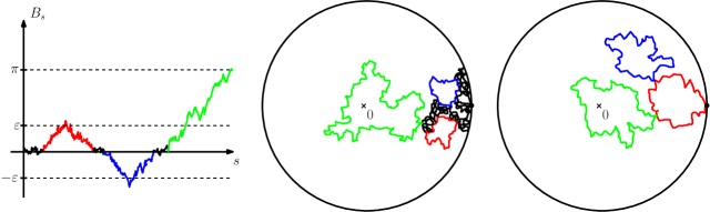
Figure 3: Left: the Brownian motion $(B_{s})_{s\geq 0}$. Center: a radial exploration of the $\mathrm{CLE}_{4}$. The red and blue excursions of height at least $\varepsilon$ give rise to two loops which do not encircle zero and the green part of the Brownian motion generates a loop which encircles zero. Right: approximation of the radial exploration.

Let us present an approximation of this radial $\mathrm{SLE}_{4}^{\langle\mu\rangle}(-2)$. Let $n\in\mathbb{N}$. The idea is to remove intervals of time where $B$ is making tiny excursions away from zero. We set $T_{0}^{n}\coloneqq 0$ and for all $k\geq 0$,

$$\left\{\begin{array}[]{cl}R_{k+1}^{n}&=\inf\{s\geq T_{k}^{n};\ \lvert B_{s}\rvert\geq 1/2^{n}\};\\ S^{n}_{k+1}&=\sup\{s\leq R^{n}_{k+1};\ B_{s}=0\};\\ T^{n}_{k+1}&=\inf\{s\geq R^{n}_{k+1};\ B_{s}=0\}.\end{array}\right.$$

Call $e^{n}_{k}$ the $k$-th excursion associated to the interval $[S^{n}_{k},T^{n}_{k}]$. Set $\Lambda^{n}\coloneqq\sup\{k;S^{n}_{k}\leq\tau_{0}\}$ and

$$l_{k}^{n}=T^{n}_{k}-S^{n}_{k}\ \forall k<\Lambda^{n}\ ;\ l^{n}_{\Lambda^{n}}=\tau_{0}-S^{n}_{\Lambda^{n}}\ ;\ L_{k}^{n}=\sum_{1\leq j\leq k}l^{n}_{j}\ \forall k\leq\Lambda^{n}.$$

Now we define for all $k\in[\![1,\Lambda^{n}]\!]$,

$$\forall k\in[\![1,\Lambda^{n}]\!],\ \forall s\in[L^{n}_{k-1},L^{n}_{k}),\qquad(W^{\mu,n}_{0})_{s}=(W^{\mu}_{0})_{S^{n}_{k}+(s-L^{n}_{k-1})},$$

and set $D^{0,\mu,n}$ to be the radial Loewner chain with driving function $W^{\mu,n}_{0}$. This is defined up to time $\tau^{n}_{0}=L^{n}_{\Lambda^{n}}$.

Let us recall an approximation of the uniform exploration of the $\mathrm{CLE}_{4}$. Sample $(X_{k}^{n})_{k\geq 1}$ uniformly and independently on $\partial\mathbb{D}$. For all $s\in[0,\tau^{n}_{0})$, set

$$\forall k\in[\![1,\Lambda^{n}]\!],\ \forall s\in[L^{n}_{k-1},L^{n}_{k}),\qquad(W^{n}_{0})_{s}=X^{n}_{k}\exp\left(i\left(2B_{s+S^{n}_{k}}-\int_{S_{k}^{n}}^{s+S_{k}^{n}}\cot(B_{u})du\right)\right).$$ (4.3)

Let $D^{0,n}$ be the radial Loewner chain with driving function $W^{n}_{0}$. By the same argument as in Section 4 of [WW13] we know that $D^{0,n}$ converges in $\mathcal{D}$ in probability towards a uniform exploration $D^{0}$ targeted at $0$ in $\mathcal{D}$ and stopped at the time $\tau_{0}$ defined by $D^{0}_{s}={\bf D}^{0}_{s\wedge\tau_{0}}$ for all $s\geq 0$. Note that the time $\tau_{0}$ thus also corresponds to the first time at which $0$ gets encircled by a loop for the uniform exploration ${\bf D}^{0}$. Moreover, as in the beginning of Section 4 of [WW13], each loop drawn by ${\bf D}^{0}$ again corresponds to the excursion of $B$ away from $\pi\mathbb{Z}$ at the same time.

Let us show the convergence in law jointly in $z\in\mathbb{Q}^{2}\cap\mathbb{D}$ as $\mu\to\infty$ of the $\mathrm{SLE}^{\mu}_{4}(-2)$ branch towards $z$ to the uniform exploration branch towards $z$, together with the convergence of the $\mathrm{CLE}_{4}$ loops surrounding $z$ to the $\mathrm{CLE}_{4}$ loops surrounding $z$. We first show the convergence of the branch $({\bf D}^{0,\mu}_{s})_{s\geq 0}$ targeted at $0$. To show this, it suffices to check the following statement:

Proposition 4.3.

The stopped exploration branch towards zero converges:

$$(D^{0,\mu},\tau_{0},B)\mathop{\longrightarrow}\limits_{\mu\to\infty}^{(\mathrm{d})}(D^{0},\tau_{0},B),$$

where the first coordinate converges in the space $\mathcal{D}$ and where $B$ is the Brownian motion from which the $D^{0,\mu}$’s are defined (and also $D^{0}$ via the approximation).

By the iterative definition of the exploration of the (nested) $\mathrm{CLE}_{4}$ towards zero, the convergence for all time follows immediately from Proposition 4.3:

Proposition 4.4.

The whole exploration branch towards zero converges:

$$({\bf D}^{0,\mu},\tau_{0},B)\mathop{\longrightarrow}\limits_{\mu\to\infty}^{(\mathrm{d})}({\bf D}^{0},\tau_{0},B),$$

where the first coordinate converges in $\mathcal{D}$ and $B$ is the Brownian motion with which the $D^{0,\mu}$’s are defined. Notice that we also get in particular the convergence in the sense of Carathéodory of the domain ${\bf D}^{0,\mu}_{\tau_{0}}$ encircled by the outermost loop encircling $0$ towards ${\bf D}^{0}_{\tau_{0}}$.

For all $z\in\mathbb{D}\cap\mathbb{Q}^{2}$, we can define the space $\mathcal{D}_{z}$ of families of domains containing $z$ which are in $\mathcal{D}$ after applying the conformal map $w\mapsto(w-z)/(1-\bar{z}w)$, equipped by the topology induced by the topology of $\mathcal{D}$. We also denote by $\tau_{z}^{\mu}$ (resp. $\tau_{z}$) the first time at which $z$ is encircled by a loop in the radial $\mathrm{SLE}^{\langle\mu\rangle}_{4}(-2)$ targeted at $z$ (resp. in the uniform exploration $({\bf D}^{z}_{s})_{s\geq 0}$). We also denote by $B^{z,\mu}$ (resp. $B^{z}$) the Brownian motion which defines $D^{z,\mu}$ (resp. $D^{z}$) composed with the conformal map $w\mapsto(w-z)/(1-\bar{z}w)$. The time $\tau^{\mu}_{z}$ (resp. $\tau_{z}$) is then the first time at which $B^{z,\mu}$ (resp. $B^{z}$) reaches $\pm\pi$. Note that as in the case $z=0$, we can build a coupling between the explorations using the same underlying Brownian motion so that $B^{z,\mu}=B^{z}$ and $\tau^{\mu}_{z}=\tau_{z}$ for all $\mu\in\mathbb{R}$. The convergence of the other branches then follows by conformal invariance as stated just below. We endow the space of continuous real functions $\mathcal{C}(\mathbb{R}_{+},\mathbb{R})$ with the topology of the uniform convergence on compact sets.

Corollary 4.5.

For all $z\in\mathbb{D}\cap\mathbb{Q}^{2}$,

$$({\bf D}^{z,\mu},\tau^{\mu}_{z},B^{z,\mu})\mathop{\longrightarrow}\limits_{\mu\to\infty}^{(\mathrm{d})}({\bf D}^{z},\tau_{z},B^{z})\qquad\text{in }\mathcal{D}_{z}\times\mathbb{R}\times\mathcal{C}(\mathbb{R}_{+},\mathbb{R}),$$ (4.4)

Moreover, we also have the convergence of the domain encircled by the outermost loop $D^{z,\mu}_{\tau^{\mu}_{z}}$ containing $z$ towards $D^{z}_{\tau_{z}}$ in the sense of Carathéodory jointly with the above convergence.

Exactly as in [AHPS23], our proof of Proposition 4.3 goes through the approximations $D^{0,\mu,n}$ and $D^{0,n}$.

Lemma 4.6.

Let $d_{\mathcal{D}}$ be the distance on $\mathcal{D}$. We have, a.s. $\tau^{n}_{0}\rightarrow\tau_{0}$ as $n\to\infty$ and

$$\sup_{\mu\in\mathbb{R}}d_{\mathcal{D}}(D^{0,\mu,n},D^{0,\mu})\mathop{\longrightarrow}\limits_{n\to\infty}^{\text{a.s}}0.$$

Proof.

The convergence of $\tau^{n}_{0}$ stems from elementary properties of the Brownian motion. To prove the uniform convergence in $\mathcal{D}$, let us define the driving functions using the same Brownian motion $B$. Let $T>0$. By Remark 4.2, it suffices to check that if $F:\partial\mathbb{D}\times[0,T]\to\mathbb{R}$ is a continuous function, bounded in absolute value by some constant $M>0$, then a.s.

$$\int_{0}^{T}F((W^{\mu,n}_{0})_{s\wedge\tau_{0}^{n}},s)ds\mathop{\longrightarrow}\limits_{n\to\infty}\int_{0}^{T}F((W^{\mu}_{0})_{s\wedge\tau_{0}},s)ds,$$

uniformly on $\mu\in\mathbb{R}$. This follows from the convergence of $\tau^{n}_{0}$ since

$$\left\lvert\int_{0}^{T}F((W^{\mu,n}_{0})_{s\wedge\tau_{0}^{n}},s)ds-\int_{0}^{T}F((W^{\mu}_{0})_{s\wedge\tau_{0}},s)ds\right\rvert\leq 2M(\tau_{0}-\tau^{n}_{0}).$$

∎

Lemma 4.7.

Fix $n\in\mathbb{N}$. Then

$$(D^{0,\mu,n},\tau^{n}_{0},B)\mathop{\longrightarrow}\limits_{\mu\to\infty}^{(\mathrm{d})}(D^{0,n},\tau^{n}_{0},B),$$

where the first coordinate converges in $\mathcal{D}$.

Proof.

We set for all $k\in[\![1,\Lambda^{n}]\!]$, $X_{k}^{\mu,n}=(W^{\mu}_{0})_{S_{k}^{n}},$ and ${\bf X}^{\mu,n}=(X^{\mu,n}_{k})_{1\leq k\leq\Lambda^{n}}$. For the uniform exploration we set ${\bf X}^{n}=(X^{n}_{k})_{1\leq k\leq\Lambda^{n}}$. We also write ${\bf e}^{n}\coloneqq(e^{n}_{k})_{1\leq k\leq\Lambda^{n}}$ the family of the excursions of height larger than $1/2^{n}$ before time $\tau_{0}$. To prove the above lemma, it is enough to verify that

$${\bf X}^{\mu,n}\mathop{\longrightarrow}\limits_{\mu\to\infty}^{(\mathrm{d})}{\bf X}^{n}.$$ (4.5)

Indeed, we know that $W_{0}^{n}$ is defined by (4.3) and moreover for all $k\in[\![1,\Lambda^{n}]\!]$, for all $s\in[L^{n}_{k-1},L^{n}_{k})$,

$$(W^{\mu,n}_{0})_{s} =(W^{\mu}_{0})_{S^{n}_{k}}\exp\left(i\left(2B_{s+S^{n}_{k}}-2B_{S^{n}_{k}}-\int_{S^{n}_{k}}^{s+S^{n}_{k}}\cot(B_{u})du-\mu(\ell^{0}_{s}-\ell^{0}_{S^{n}_{k}})\right)\right)$$

$$=X^{\mu,n}_{k}\exp\left(i\left(2B_{s+S^{n}_{k}}-\int_{S^{n}_{k}}^{s+S^{n}_{k}}\cot(B_{u})du\right)\right).$$

Thus, if ones assumes (4.5), then we have clearly the convergence of the driving function $W^{\mu,n}_{0}$ towards $W^{n}_{0}$ in the Skorokhod $J_{1}$ topology. This entails the convergence in $\mathcal{D}$ of $(D^{0,\mu,n}_{s})_{s\geq 0}$ by Remark 4.2. Let us now prove the convergence (4.5). One can see that

$$(W_{0}^{\mu})_{S^{n}_{1}}=\exp\left(i\left(2B_{S^{n}_{1}}-\int_{0}^{S^{n}_{1}}\cot(B_{s})ds-\mu\ell^{0}_{S_{1}^{n}}\right)\right),$$

and that for all $k\geq 2$,

$$(W_{0}^{\mu})_{S^{n}_{k}}=(W_{0}^{\mu})_{S^{n}_{k-1}}\exp\left(i\left(2B_{S_{k}^{n}}-\int_{S^{n}_{k-1}}^{S^{n}_{k}}\cot(B_{s})ds-\mu(\ell^{0}_{S^{n}_{k}}-\ell^{0}_{T^{n}_{k-1}})\right)\right).$$

But the $\ell^{0}_{S^{n}_{k}}-\ell^{0}_{T^{n}_{k-1}}$’s are i.i.d. exponential random variables whose parameter $\lambda_{n}>0$ only depends on $n$ (and not on $\mu$). Thus, to conclude it suffices to see that if $E$ is an exponential random variable of parameter $\lambda_{n}>0$, then

$$(E,e^{-i\mu E})\mathop{\longrightarrow}\limits_{\mu\to\infty}^{(\mathrm{d})}(E,X^{n}_{1}),$$

where $X^{n}_{1}$ is independent from $E$, which is elementary. ∎

Proof of Proposition 4.3.

This follows by combining Lemma 4.6, Lemma 4.7 and the fact that $D^{0,n}$ converges towards the uniform exploration of the $\mathrm{CLE}_{4}$ targeted at zero. ∎

4.3 Joint convergence of the exploration branches

Before proving Proposition 4.1, let us show the convergence of the interiors of the loops drawn along the exploration.

Lemma 4.8.

Let $\varepsilon>0$. For all $i\geq 1$, let $e_{\varepsilon,i}$ be the $i$-th excursion of $B$ of height at least $\varepsilon$ away from $\pi\mathbb{Z}$ during an interval $[S_{\varepsilon,i},T_{\varepsilon,i}]$. Let $\mathcal{L}^{0,\mu}_{\varepsilon,i}$ (resp. $\mathcal{L}^{0}_{\varepsilon,i}$) denote the loop drawn by ${\bf D}^{0,\mu}$ (resp. ${\bf D}^{0}$) during the interval $[S_{\varepsilon,i},T_{\varepsilon,i}]$, so that the domain inside the loop is $\mathcal{B}^{0,\mu}_{\varepsilon,i}={\bf D}^{0,\mu}_{S_{\varepsilon,i}}\setminus\overline{{\bf D}^{0,\mu}_{T_{\varepsilon,i}}}$ (resp. $\mathcal{B}^{0}_{\varepsilon,i}={\bf D}^{0}_{S_{\varepsilon,i}}\setminus\overline{{\bf D}^{0}_{T_{\varepsilon,i}}}$). Then we have, jointly with the convergence of Proposition 4.4, for all $\varepsilon>0$,

$$\left(\mathcal{B}^{0,\mu}_{\varepsilon,i}\right)_{i\geq 1}\mathop{\longrightarrow}\limits_{\mu\to\infty}^{(\mathrm{d})}\left(\mathcal{B}^{0}_{\varepsilon,i}\right)_{i\geq 1}$$

in terms of finite dimensional distributions for the Carathéodory topology and for the Hausdorff topology for their closure.

Proof.

It suffices to prove the convergence in the sense of Carathéodory since the outermost loop surrounding a point $z$ is constant in law as $\mu\to\infty$. Let $\mu_{n}\to\infty$. By Skorokhod’s representation theorem, we assume that the convergence of Proposition 4.3 holds almost surely along $\mu_{n}$.

Let $\varepsilon>0$. It is enough to prove the convergence for the excursions before the time $\tau_{0}$. Let $i\geq 1$ such that $T_{\varepsilon,i}<\tau_{0}$. By Proposition 4.3, we know that a.s.

$$D^{0,\mu_{n}}_{S_{\varepsilon,i}}\mathop{\longrightarrow}\limits_{n\to\infty}D^{0}_{S_{\varepsilon,i}}$$ (4.6)

in the sense of Carathéodory.

Besides, let us denote by $g^{0,\mu_{n}}_{S_{\varepsilon,i}}:D^{0,\mu_{n}}_{S_{\varepsilon,i}}\to\mathbb{D}$ (resp. $g^{0}_{S_{\varepsilon,i}}:D^{0}_{S_{\varepsilon,i}}\to\mathbb{D}$) the unique conformal map such that $g^{0,\mu_{n}}_{S_{\varepsilon,i}}(0)=0$ and $(g^{0,\mu_{n}}_{S_{\varepsilon,i}})^{\prime}(0)=e^{-s}$ (resp. $g^{0}_{S_{\varepsilon,i}}(0)=0$ and $(g^{0}_{S_{\varepsilon,i}})^{\prime}(0)=e^{-s}$). Then by definition of the radial Loewner chain, we have

$$\frac{1}{(W^{\mu_{n}}_{0})_{S_{\varepsilon,i}}}g_{S_{\varepsilon,i}}^{0,\mu_{n}}\left(\mathcal{L}^{0,\mu_{n}}_{\varepsilon,i}\right)=\frac{1}{X_{i,\varepsilon}}g^{0}_{S_{\varepsilon,i}}\left(\mathcal{L}^{0}_{\varepsilon,i}\right),$$

where $X_{i,\varepsilon}$ is a uniform random variable in $\partial\mathbb{D}$ which comes from the approximation of the uniform exploration. One concludes using the fact that the $(W^{\mu_{n}}_{0})_{S_{\varepsilon,i}}$’s for $i\geq 1$ converge to independent uniform random variables on $\partial\mathbb{D}$ as in the end of the proof of Lemma 4.7, so that

$$g_{S_{\varepsilon,i}}^{0,\mu_{n}}\left(\mathcal{B}^{0,\mu_{n}}_{\varepsilon,i}\right)\mathop{\longrightarrow}\limits_{n\to\infty}g_{S_{\varepsilon,i}}^{0}\left(\mathcal{B}^{0}_{\varepsilon,i}\right)$$

in the sense of Carathéodory in distribution jointly in $i\geq 1$. By taking (4.6) into account, this ends the proof. ∎

Let us conclude this section by ending the proof of Proposition 4.1.

Proof of Proposition 4.1.

Let us first prove the convergence of the exploration branches. More precisely, we want the convergences (4.4) to hold jointly in $z\in\mathbb{D}\cap\mathbb{Q}^{2}$.

For all $\mu\in\mathbb{R}$, for all $z\neq w\in\mathbb{D}\cap\mathbb{Q}^{2}$, we define the time $\sigma_{z,w}^{\mu}$ (resp. $\sigma_{z,w}$) at which the radial $\mathrm{SLE}^{\langle\mu\rangle}_{4}(-2)$ exploration (resp. uniform exploration) towards $z$ separates $w$ from $z$ by

$$\sigma^{\mu}_{z,w}=\inf\{s\geq 0;\ w\not\in{\bf D}^{z,\mu}_{s}\}\qquad\text{(resp.}\enskip\sigma_{z,w}=\inf\{s\geq 0;\ w\not\in{\bf D}^{z}_{s}\}\text{).}$$

By the target invariance of the explorations and by the renewal property, it is enough to show that for all $z\neq w\in\mathbb{D}\cap\mathbb{Q}^{2}$ we have the convergence of the separation time

$$\sigma^{\mu}_{z,w}\mathop{\longrightarrow}\limits_{\mu\to\infty}^{(\mathrm{d})}\sigma_{z,w},$$

jointly with the convergence of the branch ${\bf D}^{z,\mu}$. Actually, by conformal invariance, it is enough to prove that for all $w\in(\mathbb{D}\cap\mathbb{Q}^{2})\setminus\{0\}$,

$$\sigma^{\mu}_{0,w}\mathop{\longrightarrow}\limits_{\mu\to\infty}^{(\mathrm{d})}\sigma_{0,w},$$ (4.7)

jointly with the convergence of the branch ${\bf D}^{0,\mu}$. The convergence of the separation time (4.7) will be easier to prove in our context than in [AHPS23]. One can first see that $\sigma^{\mu}_{0,w}$ is tight as $\mu\to\infty$. Indeed, for all $\mu\in\mathbb{R}$, let $I^{\mu}$ be the smallest integer $i\geq 1$ such that the $i$-th loop surrounding $0$ does not contain $w$. Then $\sigma^{\mu}_{0,w}$ is smaller than the time at which we draw the $I^{\mu}$-th loop. If we assumed by contradiction that $\sigma^{\mu_{n}}_{0,z}\to\infty$ as $n\to\infty$ for some sequence $\mu_{n}\to\infty$, then we would have $I^{\mu_{n}}\rightarrow\infty$ and then $w$ would be at distance zero from $0$ by the Hausdorff convergence of the domains inside the loops encircling $0$ of Lemma 4.8, absurd. Similarly, $\sigma_{w,0}^{\mu}$ is also tight as $\mu\to\infty$. Now let $\mu_{n}\to\infty$. By taking a subsequence, again denoted by $\mu_{n}$, we may assume that

$$({\bf D}^{0,\mu_{n}},\tau^{\mu_{n}}_{0},B^{0,\mu_{n}},{\bf D}^{w,\mu_{n}},\tau_{w}^{\mu_{n}},B^{w,\mu_{n}})\mathop{\longrightarrow}\limits_{n\to\infty}^{(\mathrm{d})}({\bf D}^{0},\tau_{0},B^{0},\widetilde{\bf D}^{w},\widetilde{\tau}_{w},\widetilde{B}^{w})$$ (4.8)

in $\mathcal{D}\times\mathbb{R}\times\mathcal{C}(\mathbb{R}_{+},\mathbb{R})\times\mathcal{D}_{w}\times\mathbb{R}\times\mathcal{C}(\mathbb{R}_{+},\mathbb{R})$, where $(\widetilde{\bf D}^{w},\widetilde{\tau}_{w},\widetilde{B}^{w})$ has the same law as $({\bf D}^{w},\tau_{w},B^{w})$, jointly with the convergence of the separation times

$$(\sigma^{\mu_{n}}_{0,w},\sigma^{\mu_{n}}_{w,0})\mathop{\longrightarrow}\limits_{n\to\infty}^{(\mathrm{d})}(\sigma^{*}_{0,w},\sigma^{*}_{w,0})$$ (4.9)

towards some random variables $\sigma^{*}_{0,w},\sigma^{*}_{w,0}$. For all $n\geq 0$, let $\varphi_{n}:[0,\sigma^{\mu_{n}}_{0,w}]\to[0,\sigma^{\mu_{n}}_{w,0}]$ be the continuous increasing function such that for all $s\in[0,\sigma^{\mu_{n}}_{0,w}]$, we have $B_{s}^{0,\mu_{n}}=B^{w,\mu_{n}}_{\varphi_{n}(s)}$ (given by construction of the branching exploration). One can also express $\varphi_{n}(s)$ as minus the logarithm of the conformal radius of $D^{0,\mu_{n}}_{s}$ seen from $w$. Since $\sigma^{\mu_{n}}_{w,0}$ converges in distribution, and thanks to (4.8), we may take another subsequence again denoted by $\mu_{n}$ such that for all $s\in[0,\sigma^{*}_{0,w})\cap\mathbb{Q}$, we have

$$\varphi_{n}(s)\mathop{\longrightarrow}\limits_{n\to\infty}^{(\mathrm{d})}\varphi^{*}(s)$$ (4.10)

for some increasing process $(\varphi^{*}(t))_{t\in[0,\sigma^{*}_{0,w})\cap\mathbb{Q}}$ jointly with the convergences (4.8) and (4.9). This implies that $B^{0}_{t}=\widetilde{B}^{w}_{\varphi^{*}(t)}$ for all $t\in[0,\sigma^{*}_{0,w})\cap\mathbb{Q}$, hence $\varphi^{*}$ is strictly increasing. Similarly, we can also assume that for all $s\in[0,\sigma^{*}_{w,0})\cap\mathbb{Q}$, jointly with (4.8), (4.9) and (4.10), we have

$$\varphi_{n}^{-1}(s)\mathop{\longrightarrow}\limits_{n\to\infty}^{(\mathrm{d})}\psi^{*}(s)$$ (4.11)

for some increasing process $(\psi^{*}(s))_{s\in[0,\sigma^{*}_{w,0})\cap\mathbb{Q}}$. For all $s\in[0,\sigma^{*}_{w,0})\cap\mathbb{Q}$, we also have $B^{0}_{\psi^{*}(s)}=\widetilde{B}^{w}_{s}$. So $B^{0}_{|[0,\sigma^{*}_{0,w}]}$ is obtained as a time change of $\widetilde{B}^{z}_{|[0,\sigma^{*}_{w,0}]}$, which is itself a time change of $B^{0}_{|[0,\sigma^{*}_{0,w}]}$ Thus, $\varphi^{*}$ and $\psi^{*}$ can be extended to continuous increasing bijections between $[0,\sigma^{*}_{0,w}]$ and $[0,\sigma^{*}_{w,0}]$ such that $\varphi^{*}=(\psi^{*})^{-1}$. As a result, the convergences (4.10) and (4.11) hold uniformly on the corresponding intervals.

For all $\varepsilon>0$, for all $i,n\geq 1$, let $[S^{0,\mu_{n}}_{\varepsilon,i},T^{0,\mu_{n}}_{\varepsilon,i}]$ (resp. $[S^{0}_{\varepsilon,i},T^{0}_{\varepsilon,i}]$, $[S^{w,\mu_{n}}_{\varepsilon,i},T^{w,\mu_{n}}_{\varepsilon,i}]$, $[\widetilde{S}^{w}_{\varepsilon,i},\widetilde{T}^{w}_{\varepsilon,i}]$) be the interval of the $i$-th excursion of $B^{0,\mu_{n}}$ (resp. $B^{0}$, $B^{w,\mu_{n}}$, $\widetilde{B}^{w}$) of height larger than $\varepsilon$, during which the exploration ${\bf D}^{0,\mu_{n}}$ (resp. ${\bf D}^{0}$, ${\bf D}^{w,\mu_{n}}$, ${\bf D}^{w}$) draws a loop encircling a domain $\mathcal{B}^{0,\mu_{n}}_{\varepsilon,i}$ (resp. $\mathcal{B}^{0}_{\varepsilon,i}$, $\mathcal{B}^{w,\mu_{n}}_{\varepsilon,i}$, $\widetilde{\mathcal{B}}^{w}_{\varepsilon,i}$). We may assume by Lemma 4.8 that these domains converge: for all $\varepsilon>0$, jointly with the previous convergences,

$$\left(\mathcal{B}^{0,\mu_{n}}_{\varepsilon,i},\mathcal{B}^{w,\mu_{n}}_{\varepsilon,i}\right)_{i\geq 1}\mathop{\longrightarrow}\limits_{n\to\infty}^{(\mathrm{d})}\left(\mathcal{B}^{0}_{\varepsilon,i},\widetilde{\mathcal{B}}^{w}_{\varepsilon,i}\right)_{i\geq 1}$$

in the sense of Carathéodory and also for the Hausdorff distance when we consider their closure. Notice that, by the convergence of the Brownian motions, we also have the convergence of the times of start and end of the excursions of height larger than $\varepsilon$. By Skorokhod’s representation theorem, we assume that all these convergences hold almost surely.

If $s<\sigma_{0,w}$, then $w\in{\bf D}^{0}_{s}$, so that for $n$ large enough we have $w\in{\bf D}^{0,\mu_{n}}_{s}$, hence $s<\sigma_{0,w}^{\mu_{n}}$. Thus we have plainly $\sigma^{*}_{0,w}\geq\sigma_{0,w}$. Let us now prove that $\sigma^{*}_{0,w}\leq\sigma_{0,w}$. Let $\varepsilon>0$ small enough so that we can find $i\geq 1$ such that $S^{0}_{\varepsilon,i}<T^{0}_{\varepsilon,i}<\sigma^{*}_{0,w}$. Let $s<S^{0}_{\varepsilon,i}$. Then we have by definition of the exploration $\mathcal{B}^{0}_{\varepsilon,i}\subset{\bf D}^{0}_{s}$ and $\widetilde{\mathcal{B}}^{w}_{\varepsilon,i}\subset\widetilde{\bf D}^{w}_{\varepsilon,i}$. But since $T^{0}_{\varepsilon,i}<\sigma^{*}_{0,w}$ we have for all $n$ large enough $T^{0,\mu_{n}}_{\varepsilon,i}<\sigma^{\mu_{n}}_{0,w}$. Thus, for all $n$ large enough, $\mathcal{B}^{0,\mu_{n}}_{\varepsilon,i}=\mathcal{B}^{w,\mu_{n}}_{\varepsilon,i}$ (given that $B^{0,\mu_{n}}_{s}=B^{w,\mu_{n}}_{\varphi_{n}(s)}$ for all $s\leq\sigma^{\mu_{n}}_{0,w}$). Hence $\mathcal{B}^{0}_{\varepsilon,i}=\widetilde{\mathcal{B}}^{w}_{\varepsilon,i}$ a.s. by the Hausdorff convergence. Therefore ${\bf D}^{0}_{s}\cap\widetilde{\bf D}^{w}_{\varphi^{*}(s)}\neq\emptyset$ almost surely. But then by taking some $z\in{\bf D}^{0}_{s}\cap\widetilde{\bf D}^{w}_{\varphi^{*}(s)}$, we see by the Carathéodory convergence that the limits of ${\bf D}^{0,\mu_{n}}_{s}={\bf D}^{w,\mu_{n}}_{\varphi_{n}(s)}$ coincide, i.e. that ${\bf D}^{0}_{s}=\widetilde{\bf D}^{w}_{\varphi^{*}(s)}$. As a consequence, $s<\sigma_{0,w}$. By taking $\varepsilon$ small enough and $i$ such that $S_{\varepsilon,i}^{0}$ is close enough to $\sigma^{*}_{0,w}$ we obtain that $\sigma^{*}_{0,w}\leq\sigma_{0,w}$, hence (4.7). This concludes the proof since the domains $D^{z,w,\mu_{n}}_{s}$ for $s\geq 0$ correspond up to a time-change to the branch ${\bf D}^{w,\mu_{n}}$ stopped when $z$ and $w$ are separated. ∎

5 Conformally invariant distance and quantum natural distance

This section is devoted to the relationships between the distance $\mathrm{d}_{\mathrm{WW}}$ to the boundary of [WW13] and the quantum natural distance $\mathrm{d}_{\mathrm{q}}$ introduced by [AHPS23]. We prove Theorem 1.2 using Theorem 1.1, which relates these two distances via a Lamperti type transform modulo a process with stationary increments.

Proof of Theorem 1.2.

Let $\tau$ be defined by (1.2) with $\alpha=-1$. We know from Theorem 1.1 that

$$({\mathcal{Y}}({\sigma(t)}))_{t\geq 0}\mathop{=}\limits^{(\mathrm{d})}(e^{\xi(\tau(t))})_{t\geq 0},$$

so that $(\log(\mathcal{Y}(\sigma(\tau^{-1}(t)))))_{t\geq 0}$ has the same law as $\xi$ and we identify the two processes using an appropriate coupling. By (2.2) and by the fact that the Poisson point process (PPP) of loops $(\hat{\gamma}_{u})_{u\geq 0}$ of intensity $M$ introduced in Subsection 2.1 has an infinite intensity, we get that $u\mapsto\mathrm{d}_{\mathrm{q}}(\partial\mathbb{D},C_{u})$ is increasing, so that $t\mapsto\sigma(t)$ is continuous. Similarly, since the Lévy measure of $\xi$ is infinite, $t\mapsto\sigma(t)$ is increasing.

To end the proof, it is enough to show that the process $(\sigma(\tau^{-1}(t)))_{t\geq 0}$ has stationary increments. Let us denote by $(\mathcal{E}_{t})_{t\geq 0}$ (resp. $(\mathcal{F}_{u})_{u\geq 0}$) the augmented natural filtration of the càdlàg process $(\mathcal{Y}(\sigma(t)))_{t\geq 0}$ (resp. $(\mathcal{Y}(u))_{u\geq 0}$). One can write

$$(\Delta_{+}\log(\mathcal{Y}(u)))_{u\geq 0}=(\Delta_{+}\log(\nu^{2}_{h^{2}}(\partial C_{u})))_{u\geq 0}.$$

Each positive jump at some time $u$ corresponds to the discovery of a simple loop $F_{u}^{-1}(\hat{\gamma}_{u})$ where $(\hat{\gamma}_{u})_{u\geq 0}$ is a PPP which has the same law as described in Subsection 2.1 and $F_{u}:C_{u}\to\mathbb{D}$ is the conformal transformation which is given by $F_{u}=\Phi\circ\hat{F}_{u}^{z_{j_{k}}}\circ\Phi^{-1}$ when $u\in[\tau_{k-1},\tau_{k})$ using the notation introduced in Subsections 2.1 and 2.3, and where $\Phi:\mathbb{H}\to\mathbb{D}$ is a fixed conformal map.

Furthermore, by Theorem 1.1, for all $t\geq 0$, conditionally on $(\mathcal{Y}(\sigma(s)))_{0\leq s\leq t}$, the unexplored region $(C_{\sigma(t)},h^{2}_{|C_{\sigma(t)}})$ is a $2$-quantum disk of quantum boundary length $\nu^{2}_{h^{2}}(\partial C_{\sigma(t)})$. In other words, conditionally on $(\mathcal{Y}(\sigma(s)))_{0\leq s\leq t}$, the quantum surface

$$\left(\mathbb{D},h\circ F_{\sigma(t)}^{-1}+2\log|(F_{\sigma(t)}^{-1})^{\prime}|-\log(\nu^{2}_{h^{2}}(\partial C_{\sigma(t)}))\right)$$

is a unit boundary $2$-quantum disk. But using the fact that $\tau^{-1}(t)$ is an $(\mathcal{E}_{t})_{t\geq 0}$-stopping time, we get that for all $t\geq 0$, conditionally on $\mathcal{E}_{\tau^{-1}(t)}$, the quantum surface

$$\left(\mathbb{D},h\circ F_{\sigma(\tau^{-1}(t))}^{-1}+2\log|(F_{\sigma(\tau^{-1}(t))}^{-1})^{\prime}|-\log(\nu^{2}_{h^{2}}(\partial C_{\sigma(\tau^{-1}(t))}))\right)$$ (5.1)

is a unit boundary $2$-quantum disk.

Besides, by (2.2) we know that $u\mapsto\sigma^{-1}(u)=\mathrm{d}_{\mathrm{q}}(\partial\mathbb{D},C_{u})$ is adapted with respect to $(\mathcal{F}_{u})_{u\geq 0}$. Moreover, for all $u\geq 0$,

$$\tau(\sigma^{-1}(u))=\int_{0}^{\sigma^{-1}(u)}\frac{dt}{\mathcal{Y}(\sigma(t))}=\int_{0}^{u}\frac{\sigma^{-1}(dv)}{\mathcal{Y}(v)}.$$

So $(\tau(\sigma^{-1}(u)))_{u\geq 0}$ is $(\mathcal{F}_{u})_{u\geq 0}$-adapted. In particular, we obtain that for all $t\geq 0$, the random variable $\sigma(\tau^{-1}(t))$ is an $(\mathcal{F}_{u})_{u\geq 0}$-stopping time. As a result, given that $(\hat{\gamma}_{u})_{u\geq 0}$ is independent of $h^{2}$, we get that for all $t\geq 0$, conditionally on $\mathcal{F}_{\sigma(\tau^{-1}(t))}$, the point process $(\hat{\gamma}_{\sigma(\tau^{-1}(t))+u})_{u\geq 0}$ has the same law as $(\hat{\gamma}_{u})_{u\geq 0}$ i.e. it is a PPP of intensity $M$. In addition to that, by definition of $(F_{u})_{u\geq 0}$ from $(\hat{\gamma}_{u})_{u\geq 0}$, we have that conditionally on $\mathcal{F}_{\sigma(\tau^{-1}(t))}$, the pair $((\hat{\gamma}_{\sigma(\tau^{-1}(t))+u})_{u\geq 0},(F_{\sigma(\tau^{-1}(t))}\circ F_{\sigma(\tau^{-1}(t))+u}^{-1})_{u\geq 0})$ has the same law as $((\hat{\gamma}_{u})_{u\geq 0},(F_{u}^{-1})_{u\geq 0})$.

Thus, by taking the above observation on the quantum disk (5.1) into account, we have that conditionally on $\mathcal{E}_{\tau^{-1}(t)}\subseteq\mathcal{F}_{\sigma(\tau^{-1}(t))}$, the quantum disk (5.1) is a unit boundary length $2$-LQG disk independent of the pair $((\hat{\gamma}_{\sigma(\tau^{-1}(t))+u})_{u\geq 0},(F_{\sigma(\tau^{-1}(t))}\circ F_{\sigma(\tau^{-1}(t))+u}^{-1})_{u\geq 0})$, which has the same law as $((\hat{\gamma}_{u})_{u\geq 0},(F_{u}^{-1})_{u\geq 0})$. In other words, conditionally on $\mathcal{E}_{\tau^{-1}(t)}$, the quantum disk (5.1) is a unit boundary length $2$-LQG disk independent of $(F_{\sigma(\tau^{-1}(t))}(C_{\sigma(\tau^{-1}(t))+u}))_{u\geq 0}$, which has the same law as $(C_{u})_{u\geq 0}$.

Besides, for all $u\geq 0$,

$$\log\mathcal{Y}_{\sigma(\tau^{-1}(t))+u}-\log\mathcal{Y}_{\sigma(\tau^{-1}(t))}$$

$$=\log\left(\frac{\nu^{2}_{h^{2}}(F_{\sigma(\tau^{-1}(t))}^{-1}(F_{\sigma(\tau^{-1}(t))}(\partial C_{\sigma(\tau^{-1}(t))+u})))}{\nu^{2}_{h^{2}}(\partial C_{\sigma(\tau^{-1}(t))})}\right)$$

$$=\log\left(\nu^{2}_{h\circ F_{\sigma(\tau^{-1}(t))}^{-1}+2\log|(F_{\sigma(\tau^{-1}(t))}^{-1})^{\prime}|-\log(\nu^{2}_{h^{2}}(\partial C_{\sigma(\tau^{-1}(t))})}(F_{\sigma(\tau^{-1}(t))}(\partial C_{\sigma(\tau^{-1}(t))+u}))\right),$$

where we used (2.1) and the fact that $\nu^{2}_{h^{2}-\log b}=\nu^{2}_{h^{2}}/b$ for all $b>0$. So conditionally on $\mathcal{E}_{\tau^{-1}(t)}$, the process $(\log\mathcal{Y}_{\sigma(\tau^{-1}(t))+u}-\log\mathcal{Y}_{\sigma(\tau^{-1}(t))})_{u\geq 0}$ has the same distribution as $(\log\mathcal{Y}_{u})_{u\geq 0}$.

It is now a simple matter to check that $(\sigma(\tau^{-1}(t)))_{t\geq 0}$ has stationary increments. Indeed, let $t\geq 0$. For all $u,s\geq 0$, set

$$\widetilde{\mathcal{Y}}_{u}\coloneqq\frac{\mathcal{Y}({\sigma(\tau^{-1}(t))+u})}{\mathcal{Y}({\sigma(\tau^{-1}(t))})}\qquad\text{and}\qquad\widetilde{\xi}(s)\coloneqq\xi({t+s})-\xi(t).$$

Define $\widetilde{\sigma}$ from $\widetilde{\mathcal{Y}}$ as $\sigma$ is defined from $\mathcal{Y}$. Notice that $\widetilde{\xi}$ is characterized by the equality

$$\forall s\geq 0,\qquad\log\left(\widetilde{\mathcal{Y}}\left({\widetilde{\sigma}\left(\int_{0}^{s}e^{\widetilde{\xi}(r)}dr\right)}\right)\right)=\widetilde{\xi}(s).$$ (5.2)

Since $(\log\mathcal{Y}_{\sigma(\tau^{-1}(t))+u}-\log\mathcal{Y}_{\sigma(\tau^{-1}(t))})_{u\geq 0}$ has the same distribution as $(\log\mathcal{Y}_{u})_{u\geq 0}$, we obtain that

$$\left((\log\mathcal{Y}_{\sigma(\tau^{-1}(t))+u}-\log\mathcal{Y}_{\sigma(\tau^{-1}(t))})_{u\geq 0},\widetilde{\sigma},\widetilde{\xi}\right)$$

has the same law as $(\mathcal{Y},\sigma,\xi)$. Besides, by (5.2), we have for all $s\geq 0$,

$$\log\left(\widetilde{\mathcal{Y}}\left({\widetilde{\sigma}\left(\int_{0}^{s}e^{\widetilde{\xi}(r)}dr\right)}\right)\right) =\widetilde{\xi}(s)$$

$$=\xi(t+s)-\xi(t)$$

$$=\log\mathcal{Y}({\sigma(\tau^{-1}(t+s))})-\log\mathcal{Y}({\sigma(\tau^{-1}(t))})$$

$$=\log\widetilde{Y}({\sigma(\tau^{-1}(t+s))-\sigma(\tau^{-1}(t))}).$$

As a consequence, by density of the jumps of $\mathcal{Y}$ that for all $s\geq 0$,

$$\sigma(\tau^{-1}(t+s))-\sigma(\tau^{-1}(t))={\widetilde{\sigma}\left(\int_{0}^{s}e^{\widetilde{\xi}(r)}dr\right)}$$

Using the fact that for all $s\geq 0$, we have $\tau^{-1}(s)=\int_{0}^{s}e^{\xi(r)}dr$, we conclude that $\sigma\circ\tau^{-1}$ has stationary increments. ∎

6 Scaling limit of the distances to the boundary in $3/2$-stable maps

In this section, we describe the scaling limit of the distance between large faces and the boundary in $3/2$ stable maps.

6.1 Background on $3/2$-stable maps and the peeling exploration

Recall the definition of finite $3/2$-stable maps from Subsection 1.1. If one conditions a $3/2$-stable map of perimeter $2\ell$ on having at least $n$ edges and lets $n\to\infty$, then one obtains as a local limit an infinite $3/2$-stable map of perimeter $2\ell$, whose law is written $\mathbb{P}^{(\ell)}_{\infty}$. The infinite $3/2$-stable map was studied in [BCM18] and we will rely on this work in the next subsection.

To study the distances $\mathrm{d}^{\dagger}_{\mathrm{gr}}$ and $\mathrm{d}^{\dagger}_{\mathrm{fpp}}$ on Boltzmann planar maps, a convenient tool is the peeling exploration. We only give a brief overview of its definition and we refer the interested reader to the lecture notes [Cur23] and [Bud]. It consists in discovering the faces of the map, starting from the root face $f_{r}$ by looking at each step what is behind an edge on the boundary of the explored region which is chosen according to a peeling algorithm. More precisely, we say that a map $\mathfrak{e}$ with a distinguished simple face different from $f_{r}$ called a hole is a submap (with one hole) of $\mathfrak{m}$ if one can obtain $\mathfrak{m}$ by gluing a well chosen planar map in the hole of $\mathfrak{e}$ (see Figure 4).

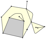
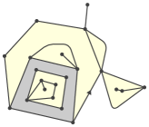
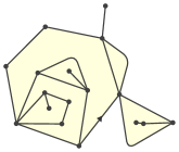
Figure 4: Left: a map $\mathfrak{e}$ with one hole which is a submap of the map $\mathfrak{m}$ on the right. The map $\mathfrak{u}$ which is in the hole of $\mathfrak{e}$ in the centre enables to recover $\mathfrak{m}$ after gluing the boundary of $\mathfrak{u}$ to the boundary of the hole.

A peeling algorithm $\mathcal{A}$ is a function which takes a submap $\mathfrak{e}$ and gives back an edge in the boundary $\partial\mathfrak{e}$ of the hole of $\mathfrak{e}$. A (filled-in) peeling exploration of $\mathfrak{m}$ is an increasing sequence $(\overline{\mathfrak{e}}_{n})_{n\geq 0}$ of submaps of $\mathfrak{m}$ starting from the submap $\overline{\mathfrak{e}}_{0}$ with only two faces which are the root face $f_{r}$ and a hole with the same degree, such that for all $n\geq 0$ the submap $\overline{\mathfrak{e}}_{n+1}$ is obtained from $\overline{\mathfrak{e}}_{n}$ as follows:

1. If the face $f$ which is on the other side of the peeled edge $\mathcal{A}(\overline{\mathfrak{e}}_{n})$ is not in $\overline{\mathfrak{e}}_{n}$, then $\overline{\mathfrak{e}}_{n+1}$ is obtained by gluing $f$ to $\overline{\mathfrak{e}}_{n}$ onto the edge $\mathcal{A}(\overline{\mathfrak{e}}_{n})$. We denote this case by $C_{k}$, where $k=\deg(f)/2$.

2. If the face $f$ on the other side of $\mathcal{A}(\overline{\mathfrak{e}}_{n})$ is already in $\overline{\mathfrak{e}}_{n}$, then $f$ must be on the boundary of the hole of $\overline{\mathfrak{e}}_{n}$ and in this case $\overline{\mathfrak{e}}_{n+1}$ is obtained by identifying the two edges on the boundary of the hole. This creates at most two holes. If $\mathfrak{m}$ is infinite, then we choose to fill in the hole which contains a finite part of the map. If $\mathfrak{m}$ is finite, we choose here to fill in the hole which has the smallest degree and in case of equality we choose to fill in a hole chosen arbitrarily (so that in the finite case we explore the locally largest component). This case is written $G_{k,*}$ or $G_{*,k}$, where $2k$ is the degree of the hole which is filled-in, depending on whether the filled-in hole is on the left or on the right of the peeled edge. If there is not any hole, then the exploration stops.

   

   

   

   

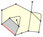
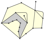
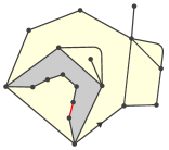
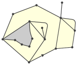
   Figure 5: From left to right: two peeling steps of the map $\mathfrak{m}$ from Figure 4 starting from the submap $\mathfrak{e}$ on the left. The red edge on the left is the edge chosen by the peeling algorithm. The peeling of the red edge causes an event of type $C_{4}$. The peeling algorithm then chooses another edge on the boundary which is again in red. When we peel this edge, an event of type $G_{3,1}$ happens and we fill-in the hole which has the smallest perimeter with a map made in this case of only one edge.

When performing the exploration, one can keep track of the perimeter process $(P(n))_{n\geq 0}$, where for all $n\geq 0$, the integer $P(n)$ is the half degree of the hole of $\overline{\mathfrak{e}}_{n}$. Notice that on an event of type $C_{k}$ for $k\geq 1$, the perimeter process increases by $k-1$ while on an event of type $G_{*,k}$ or $G_{k,*}$ for some $k\geq 0$, the perimeter process decreases by $k+1$.

A peeling algorithm which is particularly well suited to the study of the distance $\mathrm{d}_{\mathrm{fpp}}^{\dagger}$ is the uniform peeling algorithm. Given a submap $\mathfrak{e}$, it chooses uniformly at random an edge in $\partial{e}$. Using this algorithm properly coupled with the exponential random lengths defining $\mathrm{d}_{\mathrm{fpp}}^{\dagger}$, by the elementary properties of exponential random variables, one can see that for all $n\geq 0$, assuming that the exploration has not stopped before, the fpp distance from $f_{r}$ to the hole $\mathfrak{u}_{n}$ of $\overline{\mathfrak{e}}_{n}$ can be written

$$T({n+1})\coloneqq\mathrm{d}^{\dagger}_{\mathrm{fpp}}(f_{r},\mathfrak{u}_{n})=\sum_{i=0}^{n}\frac{\mathcal{E}_{i}}{2P(i)},$$ (6.1)

where the $\mathcal{E}_{i}$’s are i.i.d. exponential random variables of parameter $1$. More precisely, $\overline{\mathfrak{e}}_{n}$ corresponds exactly to the closed ball around $f_{r}$ of radius $T(n)$ where we filled-in the holes which were filled-in during the exploration, and where $T(0)=0$ by convention. In particular, a face $f$ which is discovered at time $n$ (i.e. $f\in\mathrm{Faces}(\overline{\mathfrak{e}}_{n})\setminus\mathrm{Faces}(\overline{\mathfrak{e}}_{n-1}$)) is at distance $T(n)$ from the root face $f_{r}$. When the explored map has the law $\mathbb{P}^{(\ell)}$ or $\mathbb{P}^{(\ell)}_{\infty}$, the $\mathcal{E}_{i}$’s are independent from the perimeter process. See e.g. Section 13.1 of [Cur23] or Subsection 3.2 of [Kam23] for details.

For the dual graph distance $\mathrm{d}^{\dagger}_{\mathrm{gr}}$, an appropriate peeling algorithm is the peeling by layers algorithm $\mathcal{A}_{\mathrm{layers}}$. Given a submap $\mathfrak{e}$ of $\mathfrak{m}$, we define the height of an edge $e\in\partial\mathfrak{e}$ as the dual graph distance between $f_{r}$ and the face next to $e$ which is not in the hole. Assume that there exists an integer $h\geq 0$ such that all the edges of $\partial\mathfrak{e}$ have heights in $\left\{h,h+1\right\}$ and that the edges at height $h$ form a connected interval of $\partial{\mathfrak{e}}$ (we denote this hypothesis by (H)). Then $\mathcal{A}_{\mathrm{layers}}(\mathfrak{e})$ is defined as the leftmost edge in $\partial\mathfrak{e}$ of height $h$ (see Figure 6) and when all the edges of $\partial\mathfrak{e}$ are at the same height we choose one of them arbitrarily. Notice that $\overline{\mathfrak{e}}_{0}$ satisfies (H) and that if $\overline{\mathfrak{e}}_{n}$ satisfies (H) then with $\mathcal{A}_{\mathrm{layers}}$ the submap $\overline{\mathfrak{e}}_{n+1}$ also satisfies (H) (with $h$ increasing by zero or one). For all $n\geq 0$, let us denote by $H(n)$ the smallest height of the edges in $\partial\overline{\mathfrak{e}}_{n}$ when performing a peeling by layers exploration. The sequence $(H(n))_{n\geq 0}$ is called the height process. Notice that $H(0)=0$ and that for all $n\geq 0$, we have $H(n+1)-H(n)\in\{0,1\}$. See e.g. Section 13.2 of [Cur23] for more details.

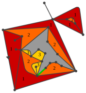
Figure 6: Illustration of the peeling by layers algorithm. The faces are colored according to their distance to the root face $f_{r}$. The edge chosen by the algorithm $\mathcal{A}_{\mathrm{layers}}$ is in green.

To be consistent with the notation of [Cur23], [BBCK18] and others, we add a subscript $\infty$ (resp. $*$) to the processes $(P(n))_{n\geq 0},(T(n))_{n\geq 0},(H(n))_{n\geq 0}$ under the law $\mathbb{P}_{\infty}^{(\ell)}$ (resp. $\mathbb{P}^{(\ell)}$). Recall that the peeling exploration under $\mathbb{P}^{(\ell)}$ satisfies a spatial Markov property in the sense that for all $n\geq 0$, conditionally on the explored region until time $n$, the maps which fill in the holes are independent Boltzmann maps, see e.g. Proposition 4.6 of [Cur23] for more details.

We finally recall from [BBCK18] the scaling limit of the perimeter process under $\mathbb{P}^{(\ell)}$ and $\mathbb{P}^{(\ell)}_{\infty}$ as $\ell\to\infty$. Let $(\Upsilon^{\uparrow}(t))_{t\geq 0}$ be a symmetric Cauchy process conditioned to stay positive and starting at $1$. More precisely, $(\Upsilon^{\uparrow}(t))_{t\geq 0}$ is the Doob $h$-transform of the Lévy process with no drift and no Brownian part, of Lévy measure $(dx/|x|){\bf 1}_{x\neq 0}$ starting at one, using the function $h(x)=\sqrt{x}$. We recall from Proposition 6.6 of [BBCK18] the following convergences in distribution for the $J_{1}$ topology of Skorokhod:

$$\text{under }\mathbb{P}^{(\ell)}_{\infty},\qquad\left(\frac{P_{\infty}(\lfloor\ell t\rfloor)}{\ell}\right)_{t\geq 0}\mathop{\longrightarrow}\limits_{\ell\to\infty}^{(\mathrm{d})}\left(\Upsilon^{\uparrow}(p_{\bf q}t)\right)_{t\geq 0};$$ (6.2)

$$\text{under }\mathbb{P}^{(\ell)},\qquad\left(\frac{P_{*}(\lfloor\ell t\rfloor)}{\ell}\right)_{t\geq 0}\mathop{\longrightarrow}\limits_{\ell\to\infty}^{(\mathrm{d})}\left(X^{(-1)}(\pi p_{\bf q}t)\right)_{t\geq 0}.$$ (6.3)

Notice here that the scaling limit of the perimeter of the locally largest component (parametrized by the exploration time) corresponds already, up to a linear time change, to the quantum boundary length of the locally largest component during a uniform or $\mathrm{SLE}^{\langle\mu\rangle}_{4}(-2)$ exploration of a $\mathrm{CLE}_{4}$-decorated quantum disk, parametrized by the quantum natural distance or the quantum length of the trunk, by Theorem 1.1.

6.2 Metric growth for infinite $3/2$-stable maps with increasing perimeter

Here we establish the scaling limit of $T_{\infty}$ and $H_{\infty}$ under $\mathbb{P}_{\infty}^{(\ell)}$ as $\ell\to\infty$. The scaling limit of $T_{\infty}$ is very easy to obtain:

Proposition 6.1.

Using the uniform peeling exploration, we have jointly with (6.2) the convergence in distribution for the topology of the uniform convergence on compact sets:

$$\text{under }\mathbb{P}^{(\ell)}_{\infty},\qquad\left(T_{\infty}(\lfloor\ell t\rfloor)\right)_{t\geq 0}\mathop{\longrightarrow}\limits_{\ell\to+\infty}^{(\mathrm{d})}\left(\int_{0}^{t}\frac{1}{2\Upsilon^{\uparrow}(p_{\bf q}s)}ds\right)_{t\geq 0}.$$

Proof.

Using (6.1) and the fact that the $\mathcal{E}_{n}$’s are independent from $P_{\infty}$, we have for all $t\geq 0$,

$$\mathbb{E}^{(\ell)}_{\infty}\left(\left.\sum_{n=0}^{\lfloor\ell t\rfloor-1}\left(\frac{\mathcal{E}_{n}-1}{2P_{\infty}(n)}\right)^{2}\right|P_{\infty}\right)=\sum_{n=0}^{\lfloor\ell t\rfloor-1}\frac{1}{\left(2P_{\infty}(n)\right)^{2}}\mathop{\longrightarrow}\limits_{\ell\to+\infty}^{(\mathbb{P})}0,$$

where the convergence comes from (6.2). Moreover, again by (6.2),

$$\text{under }\mathbb{P}^{(\ell)}_{\infty},\qquad\left(\sum_{n=0}^{\lfloor\ell t\rfloor-1}\frac{1}{2P_{\infty}(n)}\right)_{t\geq 0}\mathop{\longrightarrow}\limits_{\ell\to\infty}^{(\mathrm{d})}\left(\int_{0}^{t}\frac{1}{2\Upsilon^{\uparrow}(p_{\bf q}s)}ds\right)_{t\geq 0}.$$

This ends the proof since $t\mapsto\int_{0}^{t}1/(2\Upsilon^{\uparrow}(p_{\bf q}s))ds$ is a continuous and increasing process. ∎

For the scaling limit of $H_{\infty}$, a $\log\ell$ factor appears:

Proposition 6.2.

For the peeling by layers exploration, we have the convergence in distribution jointly with (6.2) for the topology of the uniform convergence on compact sets:

$$\text{under }\mathbb{P}^{(\ell)}_{\infty},\qquad\left(\frac{H_{\infty}(\lfloor\ell t\rfloor)}{\log\ell}\right)_{t\geq 0}\mathop{\longrightarrow}\limits_{\ell\to+\infty}^{(\mathrm{d})}\left(\int_{0}^{t}\frac{p_{\bf q}}{2\Upsilon^{\uparrow}(p_{\bf q}s)}ds\right)_{t\geq 0}.$$

To prove the above result, we will use the inverse $\theta$ of $H_{\infty}$ defined by

$$\forall k\geq 0,\qquad\theta_{k}=\inf\left\{n\geq 0,H_{\infty}(n)\geq k\right\}.$$

We will rely on the following lemma from [BCM18]:

Lemma 6.3.

(Corollary 2 of [BCM18]) For all $\varepsilon\in(0,1)$, for all $k\in\mathbb{N}$,

$$\lim_{\ell\to\infty}\mathbb{P}^{(\ell)}_{\infty}\left(\frac{p_{\bf q}\log\ell}{2\ell}\frac{\theta_{k}}{k}\leq 1+\varepsilon\right)=1.$$

We then prove Proposition 6.2.

Proof of Proposition 6.2.

This proof uses the same techniques as the proof of Proposition 6 in [BCM18], which gives a lower bound for $H_{\infty}(n)/(\log n)^{2}$ under $\mathbb{P}^{(1)}_{\infty}$ as $n\to\infty$, and will also rely on Lemma 6 of [BCM18], which bounds from above the mean increase of an interpolated version of $H_{\infty}$. Let $C>0$. For all $\ell\geq 1$ and $k\geq 0$, set $t_{k}^{(\ell)}=\lfloor C\frac{k\ell}{\log\ell}\rfloor$. Notice that

$$\Delta t^{(\ell)}_{k}\coloneqq t_{k+1}^{(\ell)}-t^{(\ell)}_{k}=(C+o(1))\frac{\ell}{\log\ell}$$ (6.4)

when $\ell\to\infty$ where the $o(1)$ is uniform in $k$. Note also that for all real $s>0$ we have

$$t^{(\ell)}_{\lfloor\frac{s\log\ell}{C}\rfloor}=\lfloor\ell s\rfloor(1+o(1))$$ (6.5)

as $\ell\to\infty$ where the $o(1)$ is non-positive.

Let $\delta\in(0,1)$. For all $\ell\geq 1$ and $k\geq 0$, let

$$\eta^{(\ell)}_{k}=\left(H_{\infty}(t^{(\ell)}_{k+1})-H_{\infty}(t^{(\ell)}_{k})-C\frac{p_{\bf q}\ell}{2P_{\infty}(t_{k}^{(\ell)})}\right){\bf 1}_{P_{\infty}(t^{(\ell)}_{k})/\ell\in[\delta,1/\delta]}.$$

Take $\varepsilon\in(0,2\delta/Cp_{\bf q})$. Let ${N}^{(\ell)}_{k}=\lfloor(1-\varepsilon)(Cp_{\bf q}\ell)/(2P_{\infty}(t^{(\ell)}_{k}))\rfloor$. Then one can see that

$$\left\{\frac{P_{\infty}(t^{(\ell)}_{k})}{\ell}\not\in[\delta,1/\delta]\right\}\cup\left(\left\{\frac{P_{\infty}(t^{(\ell)}_{k})}{\ell}\in[\delta,1/\delta]\right\}\cap\left\{{N}^{(\ell)}_{k}\leq H_{\infty}(t^{(\ell)}_{k+1})-H_{\infty}(t^{(\ell)}_{k})\right\}\right)\\ \subset\left\{\eta^{(\ell)}_{k}\geq-2\right\}.$$

Besides, by (6.4), for all $\ell$ large enough, for all $k\geq 0$, on the event $\{{P_{\infty}(t^{(\ell)}_{k})}/{\ell}\in[\delta,1/\delta]\}$, we have

$$\frac{\Delta t^{(\ell)}_{k}}{{N}^{(\ell)}_{k}}\geq\frac{2P_{\infty}(t^{(\ell)}_{k})}{(1-\varepsilon/2)p_{\bf q}\log P_{\infty}({t^{(\ell)}_{k}})}.$$ (6.6)

We define for all $\ell\geq 1$ and $k\geq 0$ the stopping times $\theta_{t_{k}^{(\ell)},0}=t_{k}^{(\ell)}$ and for all $i\geq 1$,

$$\theta_{t_{k}^{(\ell)},i}=\inf\left\{n\geq 0;\ H_{\infty}(n+t_{k}^{(\ell)})\geq H_{\infty}({t_{k}^{(\ell)}})+i\right\}.$$

Then by Lemma 6.3, for all $\gamma\in(0,1)$, for $\ell$ large enough, for all $k\geq 0$,

$$\mathbb{P}^{(\ell)}_{\infty} \left(\left\{\frac{P_{\infty}(t^{(\ell)}_{k})}{\ell}\in[\delta,1/\delta]\right\}\cap\left\{{N}^{(\ell)}_{k}\leq H_{\infty}(t^{(\ell)}_{k+1})-H_{\infty}(t^{(\ell)}_{k})\right\}\right)$$

$$=\mathbb{P}^{(\ell)}_{\infty}\left(\left\{\frac{P_{\infty}(t^{(\ell)}_{k})}{\ell}\in[\delta,1/\delta]\right\}\cap\left\{\frac{\theta_{t_{k}^{(\ell)},{N}^{(\ell)}_{k}}}{{N}^{(\ell)}_{k}}\leq\frac{\Delta t_{k}^{(\ell)}}{{N}^{(\ell)}_{k}}\right\}\right)$$

$$\geq\mathbb{P}^{(\ell)}_{\infty}\left(\left\{\frac{P_{\infty}(t^{(\ell)}_{k})}{\ell}\in[\delta,1/\delta]\right\}\cap\left\{\frac{\theta_{t_{k}^{(\ell)},{N}^{(\ell)}_{k}}}{{N}^{(\ell)}_{k}}\leq\frac{2P_{\infty}(t^{(\ell)}_{k})}{(1-\varepsilon/2)p_{\bf q}\log P_{\infty}({t^{(\ell)}_{k}})}\right\}\right)\qquad\text{by (\ref{eq delta t k sur N})}$$

$$\geq(1-\gamma)\mathbb{P}^{(\ell)}_{\infty}\left(\frac{P_{\infty}(t^{(\ell)}_{k})}{\ell}\in[\delta,1/\delta]\right),$$

the last inequality being uniform in $k$ since, under the event $\{{P_{\infty}(t^{(\ell)}_{k})}/{\ell}\in[\delta,1/\delta]\}$, the random variable ${N}^{(\ell)}_{k}$ is bounded above by $(Cp_{q})/(2\delta)$. Thus, by taking $\gamma$ arbitrarily small,

$$\lim_{\ell\to\infty}\inf_{k\geq 0}\mathbb{P}^{(\ell)}_{\infty}\left(\eta^{(\ell)}_{k}\geq-2\right)=1.$$ (6.7)

Let $s\geq 0$. Let

$$\mathcal{H}_{\ell,\delta}(s)=\frac{1}{\log\ell}\sum_{k=0}^{\lfloor(s\log\ell)/C\rfloor}(H_{\infty}(t^{(\ell)}_{k+1})-H_{\infty}(t^{(\ell)}_{k})){\bf 1}_{\forall n\in[\![t_{k}^{(\ell)},t_{k+1}^{(\ell)}]\!],\ P_{\infty}(n)/\ell\in[\delta,1/\delta]}.$$

By (6.5), we have

$$\mathcal{H}_{\delta,\ell}(s)\leq\frac{1}{\log\ell}H_{\infty}(\lfloor\ell s\rfloor)$$ (6.8)

Moreover, by (6.5) and (6.2), for all $\upsilon>0$, with probability $1-o(1)$ as $\delta\to 0$, for all $\ell$ large enough,

$$\frac{1}{\log\ell}H_{\infty}(\lfloor\ell s\rfloor)\leq\mathcal{H}_{\delta,\ell}(s+\upsilon).$$ (6.9)

Notice that with probability $1-o(1)$

One can write

$$\mathcal{H}_{\delta,\ell}(s)= \frac{1}{\log\ell}\sum_{k=0}^{\lfloor(s\log\ell)/C\rfloor}C\frac{p_{\bf q}\ell}{2P_{\infty}(t_{k}^{(\ell)})}{\bf 1}_{\forall n\in[\![t^{(\ell)}_{k},t^{(\ell)}_{k+1}]\!],\ P_{\infty}(n)/\ell\in[\delta,1/\delta]}$$

$$+\frac{1}{\log\ell}\sum_{k=0}^{\lfloor(s\log\ell)/C\rfloor}\eta^{(\ell)}_{k}{\bf 1}_{\forall n\in[\![t^{(\ell)}_{k},t^{(\ell)}_{k+1}]\!],\ P_{\infty}(n)/\ell\in[\delta,1/\delta]}.$$

Consider the first term.

$$\frac{1}{\log\ell}\sum_{k=0}^{\lfloor(s\log\ell)/C\rfloor}C \frac{p_{q}\ell}{2P_{\infty}({t_{k}^{(\ell)}})}{\bf 1}_{\forall n\in[\![t^{(\ell)}_{k},t^{(\ell)}_{k+1}]\!],\ P_{\infty}(n)/\ell\in[\delta,1/\delta]}$$

$$=\frac{1}{\log\ell}\int_{0}^{\lfloor({s\log\ell})/{C}\rfloor+1}C\frac{p_{q}\ell}{2P_{\infty}({t_{\lfloor v\rfloor}^{(\ell)}})}{\bf 1}_{\forall n\in[\![t^{(\ell)}_{\lfloor v\rfloor},t^{(\ell)}_{\lfloor v\rfloor+1}]\!],\ {P_{\infty}(n)}/{\ell}\in[\delta,\frac{1}{\delta}]}dv$$

$$=O\left(\frac{1}{\log\ell}\right)+\int_{0}^{s}\frac{p_{q}\ell}{2P_{\infty}\left({t_{\lfloor({u\log\ell})/{C}\rfloor}^{(\ell)}}\right)}{\bf 1}_{\forall n\in[\![t_{\lfloor({u\log\ell})/{C}\rfloor}^{(\ell)},t_{\lfloor({u\log\ell})/{C}\rfloor+1}^{(\ell)}]\!],\ {P_{\infty}\left(n\right)}/{\ell}\in[\delta,\frac{1}{\delta}]}du$$

$$\mathop{\longrightarrow}\limits_{\ell\to+\infty}^{(\mathrm{d})}\int_{0}^{s}\frac{p_{\bf q}}{2\Upsilon^{\uparrow}(p_{\bf q}u)}{\bf 1}_{\Upsilon^{\uparrow}(p_{\bf q}u)\in[\delta,1/\delta]}du\qquad\text{by (\ref{eq t s log ell}) and by dominated convergence.}$$

For the second term, one can see that the expectation of the negative part of $\eta^{(\ell)}_{k}$ is bounded uniformly in $\ell\geq 1,k\geq 0$:

$$\mathbb{E}^{(\ell)}_{\infty}\left((\eta^{(\ell)}_{k})_{-}\right)\leq 2+\mathbb{P}^{(\ell)}_{\infty}\left(\eta^{(\ell)}_{k}<-2\right)C\frac{p_{\bf q}}{2\delta}.$$

Hence, by (6.7),

$$\lim_{\ell\to\infty}\sup_{k\geq 0}\mathbb{E}^{(\ell)}_{\infty}\left((\eta^{(\ell)}_{k})_{-}\right)\leq 2.$$

Thus by taking $C\to\infty$, there exists a sequence of random variables $X_{\ell}$ which are stochastically dominated by $\mathcal{H}_{\delta,\ell}(s)$ such that $X_{\ell}$ converges in distribution towards $\int_{0}^{s}({p_{\bf q}}/({2\Upsilon^{\uparrow}(p_{\bf q}u)})){\bf 1}_{\Upsilon^{\uparrow}(p_{\bf q}u)\in[\delta,1/\delta]}du$.

Let us then give an upper bound in expectation of $\mathcal{H}_{\delta,\ell}(s)$. By Lemma 6 of [BCM18], for all $\varepsilon^{\prime}>0$, there exists a constant $C^{\prime}>0$ such that for all $\ell\geq 1$ and $k\geq 0$,

$$\mathbb{E}^{(\ell)}_{\infty} \left(\left(H_{\infty}(t^{(\ell)}_{k+1})-H_{\infty}(t^{(\ell)}_{k})\right){\bf 1}_{\forall n\in[\![t_{k}^{(\ell)},t_{k+1}^{(\ell)}]\!],\ P_{\infty}(n)/\ell\in[\delta,1/\delta]}\right)$$

$$\leq 2+(1+\varepsilon^{\prime})^{3}\frac{p_{\bf q}}{2}\sum_{n=t^{(\ell)}_{k}}^{t^{(\ell)}_{k+1}-1}\mathbb{E}^{(\ell)}_{\infty}\left(\frac{\log P_{\infty}(n)+C^{\prime}}{P_{\infty}(n)}{\bf 1}_{P_{\infty}(n)/\ell\in[\delta,1/\delta]}\right).$$

As a result, by (6.5),

$$\mathbb{E}^{(\ell)}_{\infty}\left(\mathcal{H}_{\delta,\ell}(s)\right)\leq\frac{1}{\log\ell}\left(2\left\lfloor\frac{s\log\ell}{C}\right\rfloor+2+(1+\varepsilon^{\prime})^{3}\frac{p_{\bf q}}{2}\sum_{n=0}^{\lfloor s\ell\rfloor-1}\mathbb{E}^{(\ell)}_{\infty}\left(\frac{\log P_{\infty}(n)+C^{\prime}}{P_{\infty}(n)}{\bf 1}_{P_{\infty}(n)/\ell\in[\delta,1/\delta]}\right)\right).$$

Thus, using (6.2), by dominated convergence as $\ell\to\infty$, and then by letting $\varepsilon^{\prime}\to 0$ and $C\to\infty$, we get that for all $\delta>0$,

$$\limsup_{\ell\to\infty}\mathbb{E}^{(\ell)}_{\infty}\left(\mathcal{H}_{\delta,\ell}(s)\right)\leq\mathbb{E}\left(\int_{0}^{s}\frac{p_{\bf q}}{2\Upsilon^{\uparrow}(p_{\bf q}v)}{\bf 1}_{\Upsilon^{\uparrow}(p_{\bf q}v)\in[\delta,1/\delta]}dv\right).$$ (6.10)

Besides, by the lower bound on $\mathcal{H}_{\delta,\ell}(s)$ and by Skorokhod’s representation theorem, we may assume that the $\mathcal{H}_{\delta,\ell}(s)$’s are defined on the same probability space and that a.s.

$$\liminf_{\ell\to\infty}\mathcal{H}_{\delta,\ell}(s)\geq\mathcal{H}_{\delta}(s)\coloneqq\int_{0}^{s}\frac{p_{\bf q}}{2\Upsilon^{\uparrow}(p_{\bf q}v)}{\bf 1}_{\Upsilon^{\uparrow}(p_{\bf q}v)\in[\delta,1/\delta]}dv.$$ (6.11)

But by Fatou’s lemma, we deduce that

$$\mathbb{E}\mathcal{H}_{\delta}(s)\leq\liminf_{\ell\to\infty}\mathbb{E}\mathcal{H}_{\delta,\ell}(s)\leq\limsup_{\ell\to\infty}\mathbb{E}\mathcal{H}_{\delta,\ell}(s)\leq\mathbb{E}\mathcal{H}_{\delta}(s),$$

where the last inequality stems from (6.10), hence $\lim_{\ell\to\infty}\mathbb{E}\mathcal{H}_{\delta,\ell}(s)=\mathbb{E}\mathcal{H}_{\delta}(s)$. Moreover, notice that for all $\varepsilon^{\prime}>0$, by dominated convergence and by (6.11),

$$\mathbb{E}\left((\mathcal{H}_{\delta}(s)-\mathcal{H}_{\delta,\ell}(s))_{+}\right) \leq\varepsilon^{\prime}+\mathbb{E}\left((\mathcal{H}_{\delta}(s)-\mathcal{H}_{\delta,\ell}(s)){\bf 1}_{\mathcal{H}_{\delta}(s)-\mathcal{H}_{\delta,\ell}(s)>\varepsilon^{\prime}}\right)$$

$$\leq\varepsilon^{\prime}+\mathbb{E}\left(\mathcal{H}_{\delta}(s){\bf 1}_{\mathcal{H}_{\delta}(s)>\mathcal{H}_{\delta,\ell}(s)+\varepsilon^{\prime}}\right)\mathop{\longrightarrow}\limits_{\ell\to+\infty}\varepsilon^{\prime}.$$

Now, since for all $x\in\mathbb{R}$, $|x|=-x+2x_{+}$, we get that $\mathbb{E}|\mathcal{H}_{\delta}(s)-\mathcal{H}_{\delta,\ell}(s)|\longrightarrow 0$ as $\ell\to\infty$. Using (6.8) and (6.9), this concludes the proof.

∎

6.3 Large $3/2$-stable maps and $\mathrm{CLE}_{4}$-decorated quantum disks

We first derive the analogues of Propositions 6.1 and 6.2 for finite $3/2$-stable maps by absolute continuity.

Corollary 6.4.

For the uniform peeling, jointly with (6.2) we have the convergence

$$\text{under }\mathbb{P}^{(\ell)},\qquad\left(T_{*}(\ell t)\right)_{t\geq 0}\mathop{\longrightarrow}\limits_{\ell\to+\infty}^{(\mathrm{d})}\left(\int_{0}^{t}{1\over 2X^{(-1)}(\pi p_{\bf q}s)}ds\right)_{t\geq 0}.$$

For the peeling by layers, jointly with (6.2) we have the convergence

$$\text{under }\mathbb{P}^{(\ell)},\qquad\left({H_{*}(\ell t)\over\log\ell}\right)_{t\geq 0}\mathop{\longrightarrow}\limits_{\ell\to+\infty}^{(\mathrm{d})}\left(\int_{0}^{t}{p_{\bf q}\over 2X^{(-1)}(\pi p_{\bf q}s)}ds\right)_{t\geq 0}.$$

Then the convergences (1.3) and (1.4) are clearly a consequence of the above corollary.

Proof.

It follows by mimicking the proof of Proposition 6.6 of [BBCK18]: by Proposition 6.3 of [BBCK18], for all $\ell\geq 1$, the Radon-Nikodym derivative of the law of the processes $(P_{*},T_{*},H_{*})$ until some time $n\geq 0$ under $\mathbb{P}^{(\ell)}$ with respect to the law of $(P_{\infty},T_{\infty},H_{\infty})$ until time $n$ under $\mathbb{P}^{(\ell)}_{\infty}$ is given by $f^{\uparrow}(\ell)/f^{\uparrow}(P_{\infty}(n))$ times the indicator function that $P_{\infty}$ does not make any negative jump of size larger than its half, where $f^{\uparrow}(\ell)\coloneqq h^{\uparrow}(\ell)/(W^{(\ell)}c_{\bf q}^{-\ell})$ and $h^{\uparrow}(\ell)=2\ell 2^{-\ell}\binom{2\ell}{\ell}$. One concludes using Propositions 6.1 and 6.2, together with the convergence in distribution of $f^{\uparrow}(\ell)/f^{\uparrow}(P_{\infty}(\ell t))$ towards $\Upsilon^{\uparrow}(p_{\bf q}t)^{-5/2}$ which comes from (1.1), and identifying the Radon-Nikodym derivative of the law of $(X^{(-1)}(\pi p_{\bf q}s))_{0\leq s\leq t}$ with respect to the law of $(\Upsilon^{\uparrow}(p_{\bf q}s))_{0\leq s\leq t}$ by Proposition 4.1 of [BBCK18]. ∎

Let us now consider the whole exploration tree in order to prove Theorem 1.3: instead of filling-in the holes, we run new explorations inside. Let us focus on the dual graph distance $\mathrm{d}^{\dagger}_{\mathrm{gr}}$, using the peeling by layers algorithm.

Recall the recursive definition of the discrete perimeter cell-system $\left((P_{u}(k))_{k\geq 0}\right)_{u\in\mathbb{U}}$ associated with a branching peeling exploration of a finite map $\mathfrak{m}$, where $\mathbb{U}=\bigcup_{n\geq 0}(\mathbb{N}^{*})^{n}$ is the Ulam tree. The process $P_{\emptyset}$ is the (half-)perimeter process of the locally largest cycle. We denote by $(N_{j})_{j\geq 1}$ the times of negative jumps of $P_{\emptyset}$ (usually ranked in the non-increasing order of jump sizes and in the decreasing order of jump times if the jump sizes are equal). Each one corresponds to an event of type $G_{k_{1},k_{2}}$, i.e. to a splitting of the distinguished hole of half-perimeter $P_{\emptyset}(N_{j})$ into two holes of half-perimeters $P_{\emptyset}(N_{j}+1)$ and $\Delta_{-}P_{\emptyset}(N_{j}):=P_{\emptyset}(N_{j})-P_{\emptyset}(N_{j}+1)-1\leq P_{\emptyset}(N_{j}+1)$. We then define $(P_{j}(k))_{k\geq 0}$ as the perimeter process of the locally largest cycle during the exploration of the submap filling the second hole. We then define $P_{uj}$ from $P_{u}$ and the time of negative jump $N_{uj}$ in the same way for all $u\in\mathbb{U}$. The birth time $B_{u}$ of the cell $u\in\mathbb{U}$ is defined recursively by $B_{\emptyset}=0$ and for all $u\in\mathbb{U},j\in\mathbb{N}^{*}$, we set $B_{uj}=B_{u}+N_{uj}$. For all $u\in\mathbb{U}$, let $\mathcal{C}_{u}$ be the cycle (i.e. the boundary of the hole) created during the birth of the cell $u$, with by convention $\mathcal{C}_{\emptyset}$ being the boundary of the root face.

Let $X$ be a self-similar Markov process such that $0$ is an absorbing state which tends a.s. towards zero or is a.s. absorbed at zero after a finite time. Let $P_{x}$ be the law of $X$ starting from $x\in\mathbb{R}_{+}$. We say that $(X_{u})_{u\in\mathbb{U}}$ is a (continuous) cell-system associated with $X$ starting at $x\geq 0$ if $X_{\emptyset}$ follows the law $P_{x}$ and for all $u\in\mathbb{U}$, conditionally on $X_{u}$, if we write $((x_{j},\beta_{uj}))_{j\geq 1}$ the family of negative jumps of $X_{u}$, where $x_{j}>0$ is the size of the jump and $\beta_{uj}$ is the time of jump, ordered in the non increasing lexicographic order ($x_{j}\geq x_{j+1}$ and if $x_{j}=x_{j+1}$ then $\beta_{j}>\beta_{j+1}$), then the $X_{uj}$ for $j\geq 1$ are independent of laws $P_{x_{j}}$. Let $\left((\mathcal{X}_{u}(t))_{t\geq 0},(\beta_{uj})_{j\geq 1},b_{u},\zeta_{u}\right)_{u\in\mathbb{U}}$ be the continuous cell-system associated with the self-similar Markov process $X^{(-1)}$.

Recall the definition of the $J_{1}$ Skorokhod topology on the space of families of càdlàg functions indexed by $\mathbb{U}$ denoted by $\mathbb{D}(\mathbb{R}_{+},\mathbb{R})^{\mathbb{U}}$ : $(f_{u}^{(n)}(t))_{t\geq 0,u\in\mathbb{U}}$ converges towards $(f_{u}(t))_{t\geq 0,u\in\mathbb{U}}$ if for all finite subset $F\subset\mathbb{U}$, $(f_{u}^{(n)}(t))_{t\geq 0,u\in F}$ converges towards $(f_{u}(t))_{t\geq 0,u\in F}$ in the space $\mathbb{D}(\mathbb{R}_{+},\mathbb{R}^{F})$ for the $J_{1}$ Skorokhod topology.

Lemma 6.5.

The rescaled dicrete cell-system associated with $\mathfrak{M}^{(\ell)}$ converges in distribution to the continuous cell-system as a random variable with values in $\mathbb{D}(\mathbb{R}_{+},\mathbb{R})^{\mathbb{U}}$ equipped with the $J_{1}$ Skorokhod topology:

$$\text{under }\mathbb{P}^{(\ell)},\qquad\left(\left(\frac{P_{u}(\ell t)}{\ell}\right)_{t\geq 0}\right)_{u\in\mathbb{U}}\mathop{\longrightarrow}\limits_{\ell\to+\infty}^{(\mathrm{d})}\left(\left(\mathcal{X}_{u}(\pi p_{\bf q}t)\right)_{t\geq 0}\right)_{u\in\mathbb{U}}.$$ (6.12)

Proof.

The proof is the same as the proof of Lemma 17 in [BCK18]. The first step is to show that the convergence (6.3) holds in the space $\mathbb{D}([0,\infty])$ equipped with Skorokhod’s $J_{1}$ topology. To prove this, it suffices to control $P_{*}(\ell t)/\ell$ for large $t\geq 0$ uniformly in $\ell$ using the supermartingale $(f^{\uparrow}(P_{*}(n)))_{n\geq 0}$ under $\mathbb{P}^{(\ell)}$ coming from Proposition 6.4 of [BBCK18], where $f^{\uparrow}$ is defined in the proof of Corollary 6.4. Then (6.12) stems from the spatial Markov property and from the fact that the $\mathcal{X}_{u}$’s for $u\in\mathbb{U}$ have a.s. no common jump times, using Proposition 2.2 page 338 of [JS87]. ∎

At this point, we are in position to prove the main result of this section.

Proof of Theorem 1.3.

We first extend the convergence (6.12) to the height processes. For every $u\in\mathbb{U}$, we can define $H_{u}$ the height process of the locally largest cycle during the (filled-in) exploration of the submap of $\mathfrak{m}$ contained in the hole created at the birth time of the cell $u$. Notice that $H_{\emptyset}=H_{*}$. Analogously, in the continuous setting, we write for all $u\in\mathbb{U}$, for all $t\geq 0$,

$$\mathcal{H}_{u}(t)=\int_{0}^{t}\frac{p_{\bf q}}{2\mathcal{X}_{u}(\pi p_{\bf q}s)}ds.$$

A direct consequence of Corollary 6.4 and Lemma 6.5 is the following convergence towards a family of continuous increasing processes which holds jointly with (6.12):

$$\text{under }\mathbb{P}^{(\ell)},\qquad\left(\left(\frac{H_{u}(\ell t)}{\log\ell}\right)_{t\geq 0}\right)_{u\in\mathbb{U}}\mathop{\longrightarrow}\limits_{\ell\to+\infty}^{(\mathrm{d})}\left(\left(\mathcal{H}_{u}(t)\right)_{t\geq 0}\right)_{u\in\mathbb{U}}.$$ (6.13)

The topology for which the above convergence holds is the product topology over $\mathbb{U}$ where each factor is equipped with the topology of the uniform convergence on compact sets.

Yet, the processes $H_{u}$ for $u\in\mathbb{U}$ only describe the height in the map encircled by $\mathcal{C}_{u}$. In order to describe the height in the whole map $\mathfrak{m}$, we introduce some additional notation. In the discrete setting, for all $u\in\mathbb{U}$, let $H(\mathcal{C}_{u})$ be the minimum of the heights (i.e. the distances to the root face) of the edges of the cycle $\mathcal{C}_{u}$. We also define $\widetilde{H}_{u}$ by induction: $\widetilde{H}_{\emptyset}=0$ and for all $u\in\mathbb{U},j\geq 1$, $\widetilde{H}_{uj}=\widetilde{H}^{(\ell)}_{u}+H_{u}(N_{uj})$. In the continuous setting, we define the birth heights $(b^{\mathcal{H}}_{u})_{u\in\mathbb{U}}$ by $b^{\mathcal{H}}_{\emptyset}=0$ and for all $u\in\mathbb{U}$, for all $j\geq 1$, $b_{uj}^{\mathcal{H}}=b^{\mathcal{H}}_{u}+\mathcal{H}_{u}\left({\beta_{uj}}/({\pi p_{\bf q}})\right)$.

Notice that by (6.12) and (6.13), we have jointly with (6.12) and (6.13) the convergence for the product topology

$$\text{under }\mathbb{P}^{(\ell)},\qquad\left(\frac{H_{u}(N_{uj})}{\log\ell}\right)_{u\in\mathbb{U},j\geq 1}\mathop{\longrightarrow}\limits_{\ell\to\infty}^{(\mathrm{d})}\left(\mathcal{H}_{u}\left(\frac{\beta_{uj}}{\pi p_{\bf q}}\right)\right)_{u\in\mathbb{U},j\geq 1}.$$ (6.14)

Since the peeling algorithm which is used in the exploration is the peeling by layers, for all $u\in\mathbb{U},j\geq 1$, every edge of $\mathcal{C}_{uj}$ is at distance $H_{u}(N_{uj})$ or $H_{u}(N_{uj})+1$ from $\mathcal{C}_{u}$. Therefore, for all $u\in\mathbb{U}$, we have $\widetilde{H}^{(\ell)}_{u}\leq H^{(\ell)}(\mathcal{C}_{u})\leq\widetilde{H}^{(\ell)}_{u}+|u|,$, where $|u|$ denotes the length of the word $u$. Thus (6.14) entails that, jointly with (6.12) and (6.13),

$$\left(\frac{H^{(\ell)}(\mathcal{C}_{u})}{\log\ell}\right)_{u\in\mathbb{U}}\mathop{\longrightarrow}\limits_{\ell\to+\infty}^{(\mathrm{d})}\left(b^{\mathcal{H}}_{u}\right)_{u\in\mathbb{U}}$$ (6.15)

Note that the positive jumps of the $P_{u}$’s for $u\in\mathbb{U}$ correspond to the (half) perimeters of the faces of $\mathfrak{m}$ minus one (without the root face).

Besides, notice that by the Markov property of Theorem 1.1, the cell system

$$\left((Y_{u}(t))_{t\geq 0}\right)_{u\in\mathbb{U}}\coloneqq\left(\left(\mathcal{X}_{u}(\pi t)\right)_{t\geq 0}\right)_{u\in\mathbb{U}}$$

describes the quantum boundary lengths along the exploration tree of the $\mathrm{CLE}_{4}$ decorated $2$-LQG disk, both for the uniform exploration and for the $\mathrm{SLE}_{4}^{\langle\mu\rangle}(-2)$ exploration, parametrized by the quantum natural distance for the first one and by the quantum length of the trunk for the second one. In particular, the positive jumps correspond the quantum boundary lengths of the loops, so that the quantum boundary lengths of the loops are all distinct (note that one can also see the fact that the quantum boundary lengths of the loops are distinct as a direct consequence of Theorem 1.2 of [AG23a] which gives the law of the quantum boundary lengths of the loops). Moreover, one can see that for all $\varepsilon>0$ there is a finite number of (outermost) loops of quantum boundary length larger than $\varepsilon$. It can be seen for instance as a consequence of Theorem 1.1 which shows that one can write $\mu^{2}_{h^{2}}(\mathbb{D})\geq\sum_{j\geq 1}b_{j}^{2}a_{j},$ where the $a_{j}$’s are i.i.d. of the same law as $\mu^{2}_{h^{2}}(\mathbb{D})$ and independent of the $b_{j}$’s which are the quantum boundary lengths of the (outermost) loops.

Then the desired result is a straightforward consequence of the convergences (6.12), (6.13) and (6.15). Indeed, by Skorokhod’s representation theorem, take a probability space where these convergences hold almost surely. Take $\varepsilon>0$. Let $F\subset\mathbb{U}$ be the finite set of $u$’s such that $Y_{u}$ has at least one jump of size larger than $\varepsilon$. The convergence (6.12) entails the scaling limit of the perimeter to the quantum boundary length and the scaling limit of the exploration time towards the quantum natural distance or quantum length of the trunk. Finally, the convergences (6.13) and (6.15) give the scaling limit of the height towards the Lamperti transform. ∎

Note that one can also obtain a “slicing at heights” of $3/2$-stable maps as in [BCK18] or [BBCK18]. For all $r\geq 1$, let $\mathrm{Ball}^{\dagger}_{r}(\mathfrak{m})$ be the ball of radius $r$ centred at $f_{r}$ in $\mathfrak{m}$. This ball is the submap of $\mathfrak{m}$ made by keeping the faces of $\mathfrak{m}$ which are at height at most $r$ and cutting along the edges which are adjacent on both sides to faces at distance $r$ to the root face. This ball has several holes of boundaries $\mathfrak{h}_{1}(\mathfrak{m},r),\mathfrak{h}_{2}(\mathfrak{m},r),\ldots$ ranked in the non-increasing order of perimeter. For all $i\geq 1$ and $r\geq 0$, let $L_{i}(r)$ be the perimeter of the hole $\mathfrak{h}_{i}(\mathfrak{m},r)$.

Let us recall the notions of self-similar growth-fragmentation. See Subsections 2.2 and 3.1 of [BBCK18] or Section 2 of [Ber17] for more details. If $(\mathcal{X}_{u},b_{u},\zeta_{u})_{u\in\mathbb{U}}$ is a continuous cell system associated with a self-similar Markov process $X$, for all $t\geq 0$ we set

$${\bf X}(t)=\left\{\!\!\{\mathcal{X}_{u}(t-b_{u});\ u\in\mathbb{U},\ b_{u}\leq t<b_{u}+\zeta_{u}\right\}\!\!\}$$

where the notation $\left\{\!\!\{\cdots\right\}\!\!\}$ refers to multiset. By Theorem 2 in [Ber17], the elements of ${\bf X}(t)$ can be ranked in the non-increasing order and form a sequence that tends to $0$, say $X_{1}(t)\geq X_{2}(t)\geq\ldots\geq 0$. If ${\bf X}(t)$ has only finitely many elements, say n, then we set $X_{n+1}(t)=X_{n+2}(t)=\ldots=0$. The process $({\bf X}_{t})_{t\geq 0}$ is called the growth-fragmentation process associated with $X$.

Let $\ell_{5/2}^{\downarrow}$ be the space of non-increasing sequences $(x_{i})_{i\geq 0}$ such that $\sum_{i\geq 1}x_{i}^{5/2}<\infty$. Let $\mathbb{D}(\mathbb{R}_{+},\ell_{5/2}^{\downarrow})$ be the space of càdlàg functions from $\mathbb{R}_{+}$ to $\ell^{\downarrow}_{5/2}$ equipped with the $J_{1}$ Skorokhod topology. Let ${\bf X}^{(0)}=((X^{(0)}_{i}(t))_{i\geq 1})_{t\geq 0}$ be the growth-fragmentation associated to the self-similar process $X^{(0)}$. Then, using exactly the same proof as the proof of Theorem 6.8 of [BBCK18], we obtain the following scaling limit:

.

Proposition 6.6.

Then we have the scaling limit in $\mathbb{D}(\mathbb{R}_{+},\ell_{5/2}^{\downarrow})$

$$\text{Under }\mathbb{P}^{(\ell)},\qquad\left(\left(\frac{L_{i}(s\log\ell)}{\ell}\right)_{i\geq 1}\right)_{s\geq 0}\mathop{\longrightarrow}\limits_{\ell\to\infty}^{(\mathrm{d})}\left({\bf X}^{(0)}(2\pi s)\right)_{s\geq 0}.$$

7 Discussion

7.1 Application to $O(2)$-decorated maps

Here we describe briefly how our results transfer to some critical $O(2)$ loop-decorated planar maps. Let us first recall the definition of a rigid loop-decorated map and the definition of Boltzmann $O(n)$ loop-decorated random planar maps for $n\in(0,2]$.

A loop-decorated map $(\mathfrak{m},{\bf\mathcal{L}})$ is a (rooted bipartite planar) map $\mathfrak{m}$ together with a loop configuration ${\bf L}=(\mathcal{L}_{1},\ldots,\mathcal{L}_{k})$ of disjoint unoriented simple closed paths on the dual map $\mathfrak{m}^{\dagger}$. Furthermore, the loops $\mathcal{L}_{i}$ do not go through the root face of $\mathfrak{m}$ and are rigid in the sense that they only visit quadrangles and they enter and exit the quadrangles through opposite sides. See Figure 7.

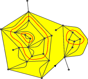
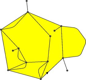
Figure 7: Left: a loop-decorated planar map. The loops, which cross quadrangles are in red. Right: its gasket, obtained by removing the interior of the outermost loops.

By convention, the distances $\mathrm{d}_{\mathrm{gr}}^{\dagger}$ and $\mathrm{d}_{\mathrm{fpp}}^{\dagger}$ are defined on a loop-decorated map by adding the rule that all the quadrangles of each loop are identified to one point, i.e. are at distance zero.

We denote the set of loop-decorated maps by $\mathcal{LM}$. For all $\ell\geq 1$, we also introduce the subset $\mathcal{LM}^{(\ell)}$ of loop-decorated maps whose root face has degree $2\ell$. Recall that ${\bf q}=(q_{k})_{k\geq 1}$ is a critical non-generic weight sequence of type $2$ in the sense that the partition function of (non-decorated rooted bipartite planar) maps $W^{(\ell)}$ behaves as in $(\ref{eq critique de type deux})$. We assume moreover, that for all $k\geq 1$,

$$q_{k}\geq\frac{2}{c_{\bf q}^{2k}}W^{(k)}.$$ (7.1)

Such a sequence does exist, as shown in Remark 1 of [Bud18] one can take for all $k\geq 1$

$$q_{k}=\frac{1}{(3\pi)^{k-1}}\left(\frac{2}{\pi}\frac{1}{(2k-3)(2k-1)}+{\bf 1}_{k=1}\right).$$

Using the so-called gasket decomposition introduced in [BBG12b, BBG12a], one can define a critical $O(2)$ Boltzmann measure $\widetilde{\mathbb{P}}^{(\ell)}$ on loop-decorated random maps of perimeter $\ell$ for all $\ell\geq 1$ in a recursive way as follows. Let $\mathfrak{M}^{(\ell)}$ be a random variable in $\mathcal{M}^{(\ell)}$ of law $\mathbb{P}^{(\ell)}$. Then, independently, on each face $f$ of $\mathfrak{M}^{(\ell)}$, with probability $(2W^{(k)})/(c_{\bf q}^{2k}q_{k})$ where $k=\deg(f)/2$, we glue quadrangles along the edges around $f$ hence forming a rigid loop and we glue in this loop an independent loop-decorated map of law $\widetilde{\mathbb{P}}^{(k)}$. The fact that $\widetilde{\mathbb{P}}^{(\ell)}$ is well defined comes from the admissibility of $\bf q$, from (7.1) and from [BBG12b] or from Theorem 1 of [Bud18]. The random loop-decorated map thus obtained is called a non-generic critical $O(n)$ loop-decorated map for $n=2$ of perimeter $\ell$ as defined at the bottom of page 4 of [Bud18]. The map $\mathfrak{M}^{(\ell)}$ is called the gasket of the obtained loop-decorated map. See Figure 7.

Using this gasket decomposition, one can see that Theorem 1.3 and Proposition 6.6 have their counterparts in terms of critical $O(2)$ loop-decorated planar maps:

• For Theorem 1.3, it suffices to replace the faces of the $3/2$-stable map by the loops of the loop-decorated map and the non-nested $\mathrm{CLE}_{4}$ by a nested $\mathrm{CLE}_{4}$. The peeling exploration becomes the peeling exploration on loop-decorated maps defined in [Bud18].

• For Proposition 6.6, one has to add a sign $(-1)^{N(\mathfrak{h})}$ to the perimeter of each hole $\mathfrak{h}$, where $N(\mathfrak{h})$ is the number of loops surrounding $\mathfrak{h}$ and one has to replace the growth-fragmentation ${\bf X}^{(0)}$ by a signed growth fragmentation as defined in [DS23], where the positive jumps give rise to cells of negative size. Notice that the obtained signed growth-fragmentation corresponds up to a Lamperti transform to the signed growth-fragmentation studied in [AdS22]. The convergence towards the growth-fragmentation holds in $\mathbb{D}(\mathbb{R}_{+},\ell^{\downarrow}_{2})$ since the harmonic functions associated to the exploration of Boltzmann planar maps which give rise to the martingales of Proposition 6.4 in [BBCK18] are replaced by the harmonic function $h^{\downarrow}_{\mathfrak{p}}$ for $\mathfrak{p}=1$ in Equation (5) of [Bud18], which is constant equal to $1$.

Besides, one can note that a similar adaptation answers Problem 4.5 of [AG23b] in the case where the gasket is a $3/2$-stable map.

However, the question of whether every critical $O(n)$ loop-decorated map’s gasket for $n=2$ is a $3/2$-stable map remains open inasmuch as the asymptotic behavior of the partition function given by Equation (3) of [Bud18] (which comes from [BBD23]) is only proven for $n\in(0,2)$.

7.2 Why the author thinks that the conformally invariant distance is not the Lamperti transform of the quantum distance

We finally argue why we believe that the conformally invariant distance to the boundary $\mathrm{d}_{\mathrm{WW}}$ of [WW13] is not the Lamperti transform $\mathrm{d}_{\mathrm{Lamperti}}$ of the quantum distance.

Let us consider, as before, a unit boundary length $2$-quantum disk $(\mathbb{D},h^{2})$ on which we draw an independent $\mathrm{CLE}_{4}$ using the uniform exploration. Let $Z$ be an independent random point of law $\mu^{2}_{h^{2}}/\mu^{2}_{h^{2}}(\mathbb{D})$ and let $\mathcal{L}$ be the (outermost) loop surrounding $Z$. By definition of the uniform exploration, conditionally on $h^{2}$ and on $Z$, the distance $\mathrm{d}_{\mathrm{WW}}(\partial\mathbb{D},\mathcal{L})$ is an exponential random variable of parameter $\lambda$ for some constant $\lambda>0$. In particular, if we stop the exploration at distance $u>0$, conditionally on not having encircled $Z$ before time $u$, the distance $\mathrm{d}_{\mathrm{WW}}(\partial\mathbb{D},\mathcal{L})-u$ from $\mathcal{L}$ to the boundary of the unexplored region is still an exponential random variable of parameter $\lambda$. On the contrary, if we stop the exploration at Lamperti transformed quantum distance $t>0$, then, conditionally on not having encircled $Z$ yet, the point $Z$ lies in each unexplored quantum disk with probability proportional to its quantum area. So the quantum disk containing $Z$ is biased by its area, so that the absence of memory for $\mathrm{d}_{\mathrm{Lamperti}}(\partial\mathbb{D},\mathcal{L})$ should be ruled out.

Nevertheless, we believe that the Lamperti transform $\mathrm{d}_{\mathrm{Lamperti}}$ of the quantum natural distance could be extended to some conformally invariant distance on the $\mathrm{CLE}_{4}$-decorated $2$-LQG disk.

Acknowledgements.

I am deeply indebted to Matthis Lehmkuehler for his guidance in the exploration of CLEs as well as in the powder snow of Les Diablerets, especially for his help for the proof of Proposition 3.1. I also thank Wendelin Werner for his advice. I am grateful to my supervisors Cyril Marzouk and Nicolas Curien for their invaluable support.

References

- [AdS22] Elie Aïdékon and William da Silva. Growth-fragmentation process embedded in a planar Brownian excursion. Probab. Theory Relat. Fields, 183(1-2):125–166, 2022.
- [AG23a] Morris Ang and Ewain Gwynne. Critical Liouville quantum gravity and CLE4, 2023. arXiv:2308.11835.
- [AG23b] Morris Ang and Ewain Gwynne. Supercritical liouville quantum gravity and CLE4, 2023. arXiv:2308.11832.
- [AHPS23] Juhan Aru, Nina Holden, Ellen Powell, and Xin Sun. Brownian half-plane excursion and critical Liouville quantum gravity. Journal of the London Mathematical Society, 107(1):441–509, 2023.
- [ASW19] Juhan Aru, Avelio Sepúlveda, and Wendelin Werner. On bounded-type thin local sets of the two-dimensional Gaussian free field. J. Inst. Math. Jussieu, 18(3):591–618, 2019.
- [BBCK18] Jean Bertoin, Timothy Budd, Nicolas Curien, and Igor Kortchemski. Martingales in self-similar growth-fragmentations and their connections with random planar maps. Probab. Theory Relat. Fields, 172(3-4):663–724, 2018.
- [BBD23] Gaëtan Borot, Jérémie Bouttier, and Bertrand Duplantier. Nesting statistics in the loop model on random planar maps, 2023. arXiv:1605.02239.
- [BBG12a] G. Borot, J. Bouttier, and E. Guitter. More on the model on random maps via nested loops: loops with bending energy. J. Phys. A, Math. Theor., 45(27):32, 2012. Id/No 275206.
- [BBG12b] G. Borot, J. Bouttier, and E. Guitter. A recursive approach to the model on random maps via nested loops. J. Phys. A, Math. Theor., 45(4):38, 2012. Id/No 045002.
- [BCK18] Jean Bertoin, Nicolas Curien, and Igor Kortchemski. Random planar maps and growth-fragmentations. Ann. Probab., 46(1):207–260, 2018.
- [BCM18] Timothy Budd, Nicolas Curien, and Cyril Marzouk. Infinite random planar maps related to Cauchy processes. J. Éc. Polytech., Math., 5:749–791, 2018.
- [Ber17] Jean Bertoin. Markovian growth-fragmentation processes. Bernoulli, 23(2):1082–1101, 2017.
- [BP] Nathanaël Berestycki and Ellen Powell. Gaussian free field, Liouville quantum gravity and Gaussian multiplicative chaos. Available on the webpages of the authors.
- [BRY19] Ilia Binder, Cristobal Rojas, and Michael Yampolsky. Carathéodory convergence and harmonic measure. Potential Anal., 51(4):499–509, 2019.
- [Bud] Timothy Budd. Peeling random planar maps (lecture notes). http://hef.ru.nl/tbudd/docs/mappeeling.pdf.
- [Bud16] Timothy Budd. The peeling process of infinite Boltzmann planar maps. Electron. J. Comb., 23(1):research paper p1.28, 37, 2016.
- [Bud18] Timothy Budd. The peeling process on random planar maps coupled to an loop model (with an appendix by Linxiao Chen), 2018. arXiv:1809.02012.
- [Cur23] Nicolas Curien. Peeling random planar maps. École d’Été de Probabilités de Saint-Flour XLIX–2019, 2023.
- [DMS21] Bertrand Duplantier, Jason Miller, and Scott Sheffield. Liouville quantum gravity as a mating of trees, volume 427 of Astérisque. Paris: Société Mathématique de France (SMF), 2021.
- [DS23] William Da Silva. Self-similar signed growth-fragmentations. Electron. J. Probab., 28:45, 2023. Id/No 49.
- [JS87] Jean Jacod and Albert N. Shiryaev. Limit theorems for stochastic processes, volume 288 of Grundlehren Math. Wiss. Springer, Cham, 1987.
- [Kam23] Emmanuel Kammerer. On large -stable maps, 2023. arXiv:2304.01167.
- [KS17] Antti Kemppainen and Stanislav Smirnov. Random curves, scaling limits and Loewner evolutions. Ann. Probab., 45(2):698–779, 2017.
- [Law05] Gregory F. Lawler. Conformally invariant processes in the plane., volume 114 of Math. Surv. Monogr. Providence, RI: American Mathematical Society (AMS), 2005.
- [Leh23] Matthis Lehmkuehler. The trunks of CLE(4) explorations. The Annals of Applied Probability, 33(5):3387 – 3417, 2023.
- [MS16] Jason Miller and Scott Sheffield. Quantum Loewner evolution. Duke Math. J., 165(17):3241–3378, 2016.
- [MSW17] Jason Miller, Scott Sheffield, and Wendelin Werner. CLE percolations. Forum Math. Pi, 5:102, 2017. Id/No e4.
- [MSW22] Jason Miller, Scott Sheffield, and Wendelin Werner. Simple conformal loop ensembles on Liouville quantum gravity. Ann. Probab., 50(3):905–949, 2022.
- [She07] Scott Sheffield. Gaussian free fields for mathematicians. Probab. Theory Relat. Fields, 139(3-4):521–541, 2007.
- [She09] Scott Sheffield. Exploration trees and conformal loop ensembles. Duke Math. J., 147(1):79–129, 2009.
- [She16] Scott Sheffield. Conformal weldings of random surfaces: SLE and the quantum gravity zipper. Ann. Probab., 44(5):3474–3545, 2016.
- [SW12] Scott Sheffield and Wendelin Werner. Conformal loop ensembles: the Markovian characterization and the loop-soup construction. Ann. Math. (2), 176(3):1827–1917, 2012.
- [SWW] Scott Sheffield, Samuel Watson, and Hao Wu. A conformally invariant metric on . Manuscript in preparation.
- [WW13] Wendelin Werner and Hao Wu. On conformally invariant CLE explorations. Commun. Math. Phys., 320(3):637–661, 2013.