Light Streak Photometry and Streaktools

Abstract

Context. The accuracy of photometric calibration has gradually become a limiting factor in various fields of astronomy, limiting the scientific output of a host of research. Calibration using artificial light sources in low earth orbit remains largely unexplored.

Aims. We aim to demonstrate that photometric calibration using light sources in low earth orbit is a viable and competitive alternative/complement to current calibration techniques, and explore the associated ideas and basic theory.

Methods. We present the publicly-available Python code Streaktools as a means to simulate and perform photometric calibration using real and simulated light streaks. We use Streaktools to perform ‘pill’ aperture photometry on 131 simulated streaks, and MCMC-based PSF model-fitting photometry on 425 simulated streaks in an attempt to recover the magnitude zeropoint of a real exposure of the DECam instrument on the Blanco 4m telescope.

Results. We show that calibration using pill photometry is too inaccurate to be useful, but that PSF photometry is able to produce unbiased and accurate (1$\sigma$ error = 3.4mmag) estimates of the zeropoint of a real image in a realistic scenario, with a reasonable light source.

1 Introduction

With the great improvement in astronomical instrumentation over the past few decades, accurate photometric calibration is becoming a limiting factor in certain fields of astronomy. The general procedure for calibration is straightforward: a source of known intensity is used to calibrate the brightness scale for an instrument under certain conditions. Certain criteria apply to these calibrators. Astronomical telescopes are focused to infinity, and so a calibration source must be far away; nearby sources would necessitate impractical refocusing of the telescope. This also implies that the sources must be very bright, so as to appear bright from larger distances. Stars and Quasars have long served as photometric standards in this manner.

Artificial sources

It is also possible to use artificial sources for photometric calibration, though the previous requirements still apply (Albert, 2012). Such an artificial source must be in the upper atmosphere, or in space. Any closer to the ground and the calibration wouldn’t be useful; one loses the ability to calibrate for a certain airmass, and observations requiring such calibration are made far above the horizon. The use of artificial light sources for calibration has several advantages. First, light sources can be engineered to very precise specifications and can have their output measured with very high precision on the ground. Secondly, man-made sources’ output can be monitored in real time using stable, calibrated onboard detectors. There are also disadvantages to this approach. Useful sources placed many tens to hundreds of kilometers away must be reasonably bright, a considerable engineering requirement for satellites or balloon payloads. Another set of disadvantages specific to satellites comes from the large motion they will have against the sky, in most orbits. This has consequences which we will explore in more detail in sections to come.

Description of following sections

In the Theory section we explore the theory of light-streak based calibration, where satellites with precise light sources are used for photometric calibration. We describe the situation mathematically with several assumptions and detail how the key object of interest, the magnitude zeropoint of the instrument under a certain set of conditions, may be recovered. We attempt to quantify uncertainties in these measurements by examining the propagation of errors due to engineering tolerances and uncertainty in satellite position. Next, we discuss methods for applying streak photometry analogous to stellar aperture and point-spread-function (PSF) photometry. In the next section, with the theory and methodology laid out, we introduce Streaktools, a set of tools implemented in Python for simulating streaks in real images using arbitrary point spread functions, and for making measurements using the discussed methods on both simulated and real streaks. The Methods, Results and Discussion sections describes our use of Streaktools to simulate to several hundred streaks and use them to recover the magnitude zeropoint of a real image, using several different implemented techniques.

2 Theory

2.1 Magnitude and zeropoints

A general expression for the apparent magnitude m of an object with an integrated flux F through some bandpass is given by

$$m=-2.5\log_{10}\biggl{(}{\frac{F}{F_{\text{ref}}}}\biggr{)}+M_{\text{ref}},$$ (1)

where $F_{\text{ref}}$ is the integrated flux of an object with apparent magnitude $M_{\text{ref}}$. Selection of $F_{\text{ref}}$ and $M_{\text{ref}}$ fixes the relationship between magnitude and flux. In CCD images (with ideally linear detector response), the number of counts $C$ received from a source is proportional to integrated flux, and so one can replace $F$ and $F_{\text{ref}}$ with a measured number of counts $C$ and some reference number of counts $C_{\text{ref}}$ which has a known magnitude $M_{\text{ref}}$. Convention is then to set $C_{\text{ref}}$ to one, and call $M_{\text{ref}}$ the magnitude zeropoint $M_{0}$; the magnitude corresponding to a single count in the image. The relation between magnitude and CCD image counts ($C$) in ADU is then

$$m=-2.5\log_{10}(C)+M_{0},$$ (2)

The goal of photometric calibration is to accurately measure $M_{0}$ so that (2) can be used to calculate all other magnitudes. $M_{0}$ can be calculated from (2) if one can know both the number of counts $C$ and associated magnitude $m$ of any source. Photometric calibration then consists of calculating or otherwise establishing the magnitude $m$ of a calibrator, and measuring the number of counts $C$ associated with the source in an image. We presently discuss the calculation of the magnitude associated with a light streak in an image.

2.2 Calculating streak magnitudes

Note that here we will be working in the AB magnitude system, the definition of which lends itself to the following calculation. $m$ can be calculated from (1), since we can calculate the expected flux $F$ of the source, and the definition of the AB system specifies $F_{\text{ref}}$ and $M_{\text{ref}}$ for us. Note that here, by integrated flux we mean power per unit area received by the instrument through the bandpass, whereas irradiance $I$ refers to the power per unit area provided by the source at the telescope aperture. We further assume that this source is very band limited, with a specific and well-known wavelength, as in a laser. The source flux may then be calculated as

$$F=I\cdot S(\lambda_{0}),$$ (3)

where $S(\lambda_{0})$ is the transmission of the bandpass at the source wavelength $\lambda_{0}$. This is not however the flux that will be measured by the telescope, which measures flux by integrating it over a length of time. Assume now that the streak is caused by a pulse of known pulse interval $\Delta t$, and that the exposure time is $T$ - the effective flux measured by the instrument $F_{\text{meas}}$ will now be

$$F_{\text{meas}}=I\cdot S(\lambda_{0})\frac{\Delta t}{T}.$$ (4)

Note that (5) implies we are not calculating the true magnitude of an artificial light source, but rather the magnitude it corresponds to in the image given that the light source was not necessarily active for the whole exposure period. In the AB magnitude system, a source is defined to have a magnitude of zero when its spectral flux density $f_{\nu}$ is approximately 3631Jy. A Jansky (Jy) is a unit of spectral flux density defined as $10^{-26}$ $W$/$m^{2}$/Hz. The total integrated flux $F_{0}$ of a (by definition) zero-magnitude source (AB system) can then be calculated as

$$F_{0}=\int S(\lambda^{\prime})f_{\lambda}(\lambda^{\prime})d\lambda^{\prime}=\int S(\nu^{\prime})(3631Jy)d\nu^{\prime},$$ (5)

where $f_{\lambda}$ is the flux per unit wavelength corresponding to the zero-magnitude spectral flux density, 3631Jy, and $S$ is the bandpass transmission profile. Since this reference flux by definition corresponds to a magnitude of zero, (1) then lets us calculate the theoretical magnitude of this source as

$$m=-2.5\log_{10}\biggl{(}\frac{F_{\text{meas}}}{F_{0}}\biggr{)},$$ (6)

where $F_{0}$ is given by (5), and $F_{\text{meas}}$ is given by (4). Finally, we need an expression for the irradiance of the source at the site of observation, to plug into (3). Here we assume the source to be an integrating sphere (IS) with a cosine intensity profile around its axis, caused by the change in the projected area of its aperture. We will call the angle between the light source axis and the source-observatory line $\theta$. Idealized integrating sphere output can be characterized by one value, the output radiance $R_{IS}$, which is the power radiated per unit projected output aperture area, per unit solid angle radiated into. The irradiance at the telescope can then be calculated using the known radiance $R_{IS}$, integrating sphere aperture area $A_{IS}$, and the distance to the satellite source, $d$:

$$I(d,\theta)=\frac{R_{IS}A_{IS}\cos(\theta)}{d^{2}}.$$ (7)

Any appropriate irradiance though may be plugged into (3) and the analysis here performed to determine the magnitude corresponding to the streak.

2.3 Streak Photometry

In this section, we describe methods for recovering the number of counts $C$ associated with a streak in a CCD image.

Pill aperture photometry

The natural extension of the ubiquitous methods of circular and elliptical aperture photometry is pill aperture photometry, pioneered by Fraser et al. (2016). With this technique, the usual circular apertures are drawn out into pill shapes to encompass streaks in astronomical images. This approach is computationally straightforward but has serious drawbacks. Pill-shaped apertures enveloping long streaks necessarily cover more sky than for a stationary source for the same flux, reducing the final signal to noise ratio (SNR). The risk of other sources in the field intersecting the streak and the pill also increases linearly with the length of the streak; these sources add unwanted flux if not source-subtracted, and remove flux or at the very least add noise even with good source subtraction. Another issue is that the larger integration area of the pill requires very accurate sky background subtraction. For example, a remaining mean sky value of just 0.05 over a pill 1400 pixels long and 30 pixels wide (typical for certain instruments) can be expected to add/subtract over 2000 unexpected counts and easily affect flux measurements for reasonable satellite sources by over 10%, ruining any calibration. These issues are severe enough that we end our analysis of this approach here. Below we detail the use of simulations to show that this approach is unfeasible.

Extending PSF photometry

Another option for photometry is to recover the number of counts by fitting a model for the streak to the data. A model can be constructed as follows: assume that the point spread function (PSF) of the observation is known. The streak model is then the convolution of a mathematical line of length $L$ passing through the image at an angle $\phi$ with the observation PSF. We offset the centroid of the streak with parameters $x_{c}$ and $y_{c}$, and then normalize the map so that it integrates to to the model count number $C$, and complete the model by adding a local sky mean $\mu_{\text{sky}}$. Expressed mathematically, this is

$$M(x,y;x_{c},y_{c},\phi,L,C,\mu_{\text{sky}})=\frac{C\cdot l(x,y)\ast\mathcal{P}(x,y)}{\int l(x^{\prime},y^{\prime})\ast\mathcal{P}(x^{\prime},y^{\prime})dx^{\prime}dy^{\prime}}+\mu_{\text{sky}}.$$ (8)

In (8), $l$ is the mathematical line corresponding to the streak, which depends on the offset parameters $x_{c}$ and $y_{c}$ , the angle parameter $\phi$, and the streak length $L$. $\mathcal{P}$ is the point spread function of the observation, and the integral is understood to be over the entire model. Our approach here is similar to that of Fraser et al. (2016) but with an expanded parameter set. The model they implement in their package ‘Trailed-Image Photometry in Python’ (TRIPPy) wisely uses fewer fitting parameters, instead constructing the trailed spread function (TSF), equivalent to the integrand in (17) from known information. For our purposes, the expanded parameters are necessary since the angle at which a satellite passes through an image and the streak length cannot generally be predicted with the required accuracy, given that the streaks formed by low earth orbit (LEO) sources are much longer than those from solar system celestial objects owing to their rate of passage through the field of view.

Fitting statistics

A typical choice for fitting a fitting statistic to be minimized, $\chi^{2}$, is not applicable in this situation. $\chi^{2}$ is only an appropriate statistic when the observed data is normally distributed, since $\chi^{2}$ is the sum of standard normal statistics $Z_{i}^{2}$ for all $i$ bins in a dataset. Our pixel counts are Poisson distributed, and even though the Poisson distribution converges to a Gaussian for high bin counts the bias introduced by minimizing using $\chi^{2}$ can still be significant (Humphrey et al., 2009). The quantity we are interested in computing accurately is the logarithm of the likelihood function $\mathcal{L}$. For our model, the likelihood function (the probability of a specific outcome defined by the set of observed pixel values $O_{i}$) is

$$\mathcal{L}=\prod_{i}\frac{E_{i}^{O_{i}}}{O_{i}!}e^{-E_{i}},$$ (9)

for expected (mean) pixel values $E_{i}$, which gives a log-likelihood function of

$$\ln(\mathcal{L})=\sum_{i}\biggl{[}O_{i}\ln(E_{i})-E_{i}-\ln(O_{i}!)\biggr{]},$$ (10)

It is often desirable to simplify this expression and reduce the time it takes for a computer to evaluate it. Specifically, the logarithm of a factorial of a potentially large number is problematic. Stirling’s approximation, $\ln(N!)\approx N\ln(N)-N$, can be applied to reach an approximation for $\ln(\mathcal{L})$ which will be very accurate when pixel values are not small:

$$\ln(\mathcal{L})\approx-\frac{C}{2}\;\;||\;\;C\equiv 2\sum_{i}\biggl{[}(E_{i}-O_{i})+O_{i}\ln\biggl{(}\frac{O_{i}}{E_{i}}\biggr{)}\biggr{]}.$$ (11)

$C$ is a statistic known as Cash’s C (Cash, 1979). $C$ is defined with the extra factor of 2 so that it converges to $\chi^{2}$ in the limit of large observed and expected values (compare to $\ln(\mathcal{L})$ for a set of Gaussian bins, $-\chi^{2}/2$). Since observed pixel values are the sum of source and sky Poisson counts, the sky brightness should be considered as part of the model when computing the likelihood of a set of pixel values. If this was ignored, the sky contribution to pixel variance (which can be large or even dominant at the edges of a source) would be missed, and comparatively likely outcomes would be considered unlikely. This can bias the outcome of maximum likelihood fitting. To correctly compute the likelihood function and perform maximum likelihood fitting it is necessary to include the sky background as a fitting parameter and work on images that have not been sky subtracted, as the sky mean influences variance of sky, and therefore total, counts. Using sky-subtracted images would necessitate the estimation of the sky mean from the local Poisson noise, which can only add error.

2.4 Fitting using MCMC

With exact (10) and approximate (11) expressions for $\ln(\mathcal{L})$, we only need a fitting algorithm. Gradient descent and similar algorithms are not safe to use for optimization in this context, since they are prone to finding local rather than global maxima in the potentially complicated likelihood function in higher dimensional parameter spaces like ours. Other algorithms exist for efficiently sampling from distributions with high-dimension parameter spaces. Markov Chain Monte-Carlo (MCMC) algorithms, such as the Metropolis-Hastings algorithm (Hastings, 1970), were designed specifically for this purpose. Such algorithms are often used for fitting models with many parameters to data. In this approach, a large number of ‘walkers’ are initialized and are iteratively moved to new states in the parameter states, with the likelihood of a new state being accepted being calculated in part using the provided likelihood function. Over enough iterations, the walkers converge to the posterior distribution defined by the likelihood function and thereby allow measurement of the most likely parameters. Here we will be using the Python package emcee (Foreman-Mackey et al., 2013), an implementation of the efficient affine-invariant ensemble sampler proposed by Goodman and Weare (Goodman & Weare, 2010).

2.5 Theoretical precision

With the procedure for zeropoint calculation established, we turn to theoretical uncertainties in our calibration given sufficiently small Gaussian uncertainties in input parameters. For a dependent quantity $f$ which is a function of the set of parameters $x_{i}$, the 1$\sigma$ uncertainty in $f$ is related to the same uncertainty in each $x_{i}$ by:

$$\sigma_{f}^{2}=\sum_{i}\biggl{(}\frac{\partial f}{\partial x_{i}}\biggr{)}^{2}\sigma_{x_{i}}^{2}.$$ (12)

Using (12), straightforward calculus and equations (2), (4) and (6) one can derive the following expression for magnitude zeropoint variance:

$$\sigma_{M_{0}}^{2}=\biggl{(}\frac{2.5}{\ln 10}\biggr{)}^{2}\biggl{[}\biggl{(}\frac{\sigma_{I}}{I}\biggr{)}^{2}+\biggl{(}\frac{\sigma_{F_{0}}}{F_{0}}\biggr{)}^{2}+\biggl{(}\frac{\sigma_{C}}{C}\biggr{)}^{2}\biggr{]}.$$ (13)

Here $I$, $F_{0}$ and $C$ respectively refer to the Satellite irradiance at the observatory, the flux zeropoint and the number of counts associated with the streak. From here, one can use (6) to break up the irradiance uncertainty into uncertainties in satellite position, orientation and engineering specifics, again using (10). We will explore this in several scenarios now.

Satellite oriented to local nadir

One orientation for the satellite during the observation is to its local nadir. In this situation, the integrating sphere axis angle $\theta$ can be expressed in terms of the altitude angle $\alpha$ of the satellite, that is the angle above the horizon which the satellite appears at as seen by the observatory, and the distance to the satellite $d$. Since the local nadir for the satellite will not be the same absolute direction as the local nadir at the observatory owing to the curvature of the Earth, the radius of the Earth $R_{e}$ shows up in the resulting expression for $\theta$:

$$\theta=\pi-\alpha-\sin^{-1}\biggl{(}\frac{\cos(\alpha)}{r_{\ast}}\biggr{)}\;\;\;||\;\;\;r_{\ast}^{2}\equiv\biggl{(}\frac{R_{e}}{d}\biggr{)}^{2}+2\biggl{(}\frac{R_{e}}{d}\biggr{)}\sin(\alpha)+1$$ (14)

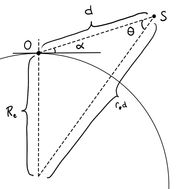
Figure 1: Nadir-oriented geometry. The position of the satellite (S) is described in relation to the observation point (O) by its altitude angle $\alpha$ and distance $d$

Applying (12) to (7) and (14) allows us to express the uncertainty in the irradiance $I$ in terms of its dependencies $A_{IS}$, $R_{IS}$, $\alpha$ and $d$, and uncertainties thereof:

$$\sigma_{I}^{2}=\biggl{(}\frac{\partial I}{\partial R_{IS}}\biggr{)}^{2}\sigma_{R_{IS}}^{2}+\biggl{(}\frac{\partial I}{\partial A_{IS}}\biggr{)}^{2}\sigma_{A_{IS}}^{2}+\biggl{(}\frac{\partial I}{\partial{\alpha}}\biggr{)}^{2}\sigma_{\alpha}^{2}+\biggl{(}\frac{\partial I}{\partial d}\biggr{)}^{2}\sigma_{d}^{2}$$ (15)

where the partial derivatives are given by

$$\frac{\partial I}{\partial R_{IS}}=\frac{I}{R_{IS}},\;\;\;\;\;\;\frac{\partial I}{\partial A_{IS}}=\frac{I}{A_{IS}},$$

$$\frac{\partial I}{\partial\alpha}=R_{IS}A_{IS}\sin(\theta)\biggl{[}1-\frac{\frac{\sin(\alpha)}{r_{\ast}}+\frac{2}{r_{\ast}^{2}}(\frac{R_{e}}{d})\cos^{2}(\alpha)}{\sqrt{1-(\frac{\cos(\alpha)}{r_{\ast}})^{2}}}\biggr{]},$$

$$\frac{\partial I}{\partial d}=-2R_{IS}A_{IS}\biggl{[}\frac{\cos(\theta)}{d^{3}}+\biggl{(}\frac{R_{e}^{2}}{d}+R_{e}\sin(\alpha)\biggr{)}\biggl{(}\frac{\sin(\theta)\cos(\alpha)}{d^{4}r_{\ast}^{2}\sqrt{1-(\frac{cos(\alpha)}{r_{\ast}})^{2}}}\biggr{)}\biggr{]}.$$

The above expressions allow one to compute the uncertainty in the magnitude zeropoint directly from uncertainties in satellite position, orientation and engineering parameters, in the case that the satellite is oriented to its local nadir.

Satellite oriented to observation site

One could also orient the satellite directly towards the observation point at the moment a calibration observation is made. This has two benefits. First, the cosine profile of the irradiance with satellite orientation is maximized when the integrating sphere aperture axis is oriented directly towards the observation point. Secondly, since the derivative of this cosine function vanishes along this axis ($\theta$ = 0), the sensitivity of the irradiance to slightly imperfect orientation also vanishes, and therefore the impact of imprecise alignment is minimized when the satellite is oriented this way. The uncertainty calculations are straightforward compared to the nadir-oriented situation. (11) still applies, but now the variance of the irradiance is given by

$$\sigma_{I}^{2}=\biggl{(}\frac{\partial I}{\partial R_{IS}}\biggr{)}^{2}\sigma_{R_{IS}}^{2}+\biggl{(}\frac{\partial I}{\partial A_{IS}}\biggr{)}^{2}\sigma_{A_{IS}}^{2}+\biggl{(}\frac{\partial I}{\partial d}\biggr{)}^{2}\sigma_{d}^{2}$$ (16)

where the partial derivatives are given by

$$\frac{\partial I}{\partial R_{IS}}=\frac{I}{R_{IS}},\;\;\;\;\;\frac{\partial I}{\partial A_{IS}}=\frac{I}{A_{IS}},\;\;\;\;\;\frac{\partial I}{\partial d}=-2\frac{R_{IS}A_{IS}}{d^{3}}.$$

It is worth noting that (12) assumes errors are small enough that dependent functions $f$ can be linearly approximated, so quadratic and higher order error may still be unaccounted for if parameter uncertainties are very large.

3 Streaktools

A description of Streaktools

So far, we have discussed the basic theory of photometric calibration, how a streak created by an artificial light source in orbit can be used to provide this calibration, and several methods for retrieving the number of counts in an image associated with a streak. Now we seek to demonstrate that realistically simulated streaks can be used for calibration by applying this theory. To this end, we have written Streaktools for Python, which allows a user to:

• generate streaks from satellite engineering specifications and position

• generate streaks with any user-defined point spread function

• add and remove realistic streaks from any real or simulated data

• perform pill aperture photometry on simulated streaks

• use emcee to fit models to data for zeropoint recovery

• apply the above methods to real streaks

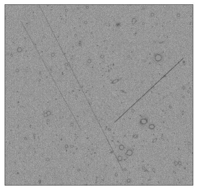
Figure 2: A real streak (longest, in the centre), and two streaks simulated and added to a Dark Energy Camera (DECam) image, using Streaktools. These streaks were both generated using the PSF recovered from the image with TRIPPy and SExtractor.

Streaktools simulates streaks using a user-defined ‘true’ magnitude zeropoint, from which the streak is generated. The true magnitude of the streak is calculated using (6), with all of the relevant parameters supplied by the user. After the true number of counts is calculated, the streak model is generated using (8), and an observation of the streak is simulated by computing pixel values as Poisson variables, with mean parameters given by the model at each point. These streaks, with any length, position and orientation may be added, removed and changed at will in data from user-supplied 2D arrays. Results of the photometric methods previously discussed are presented in an easy to read form, automatically calculating and storing the recovered magnitude zeropoints and best-fit parameters. Methods are implemented in Streaktools that tell the algorithm to ignore contributions to the likelihood function calculation beyond a certain distance from the streak, preventing bright nearby sources from skewing likelihood calculations as they are not accounted for in the model.

We do not cover the use of streaktools here; a tutorial is provided with the code which demonstrates all of its features. The code and tutorial may be found publicly accessible on github.

4 Methods

To test Streaktools and the performance of several calibration methods, we simulated random streaks and added them to data from an exposure taken on 31 Jan. 2023 using the Dark Energy Camera (DECam) instrument on the Blanco 4m telescope. These streaks were generated with lengths between 200 and 700 pixels, (clockwise from horizontal) intersection angles from 0 to 90 degrees, randomly positioned in an area covering roughly a quarter of the 2k$\times$4k pixel CCD image used. TRIPPy (Fraser et al., 2016) and Source Extractor (Bertin & Arnouts, 1996) were used to recover the point spread function of the observation using stars in the image, which was then used for streak simulation and models during calibration. Our aim is to evaluate Streaktools and the zeropoint recovery methods used, and so satellite source parameters are exactly ‘known’, but are still randomly generated. We generate satellite radiance values between 50 and 1000 W/m²/Sr, a small integrating sphere aperture of 1.27cm², generated by a satellite 600km away at an altitude angle of 45 degrees above the horizon. This corresponds to total integrating sphere output of 2mW to 400mW. First, 131 streaks were simulated in a sky-subtracted version of the data, and we tested two methods of pill aperture photometry using Streaktools:

• ‘ordinary’ pill photometry: the number of counts inside the aperture is taken to be the final measurement

• ‘compared’ pill photometry: the number of counts inside the pill is compared between the exposure with the streak and an exposure from immediately (1 minute) before, and their difference is taken as the measurement of streak flux. This is done in an effort to remove bias from background sources

A width parameter $r$ (as detailed in Fraser et al. (2016)) of 4$\times$ the FWHM of the PSF was used for all pills. Next, 425 streaks were simulated in a non sky-subtracted version of the data, and MCMC-based maximum-likelihood fitting was performed using Streaktools. For these simulations, we use 40 MCMC walkers, initialized uniformly in region of the parameter space centered on the initializing parameter values for each streak, with a spread intended to represent the accuracy within which an initial guess for the streak model parameters could be provided by a user (several pixels for position, 10 pixels for length, half a degree for angle, and a several $\sigma$ spread for counts and sky background using their Poisson statistics). For all of these simulations, we record generated streak parameters, and calibration results as reported by streaktools with associated uncertainties (estimated from sky noise, total counts and pill area for pill photometry, and from statistics of MCMC results for maximum likelihood fitting). To generate the streaks we use a preset ‘true’ magnitude zeropoint of exactly 28.88802, which is very close to the true zeropoint for the image established through stellar photometry (chosen for realism). The goal for these photometric methods is to recover this preset zeropoint accurately.

5 Results

5.1 Pill vs. PSF

We find that both forms of pill aperture photometry described yield poor results, expecially for longer streaks and when compared with the MCMC fitting results.

Table 1: Zeropoint recovery statistics for all three results

Parameter	Pill	Compared	MCMC/PSF
$\bar{x}$ (mmag)	-135	304	0.0308
$s_{x}$ (mmag)	486	411	3.41
$\sigma_{\bar{x}}$ (mmag)	42	36	0.165

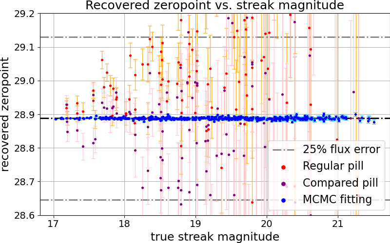
Figure 3: Recovered zeropoint vs. streak magnitude for the 3 methods

Given in table 1 are statistics for the pill photometry and MCMC/PSF photometry results (in mmag; ‘millimag’ = $10^{-3}$mag). Shown for the zeropoint error $x$ (the difference between the recovered and true zeropoint) are the mean $\bar{x}$, the standard deviation $s_{x}$, and the 1$\sigma$ uncertainty in the mean zeropoint error $\sigma_{\bar{x}}$. MCMC/PSF photometry on average recovered the true zeropoint 2 orders of magnitude more accurately than the pill methods, and did so consistent with zero bias, unlike the pill results. As intended, the compared pill photometry is not biased towards flux overestimation the way ordinary pill photometry is, but both pill methods’ results reflect impractically poor precision.

5.2 MCMC/PSF photometry results

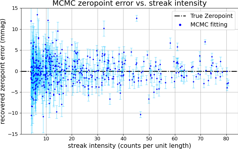
Figure 4: MCMC/PSF zeropoint error vs. streak intensity

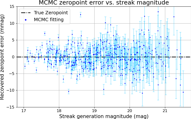
Figure 5: MCMC/PSF zeropoint error vs. streak magnitude

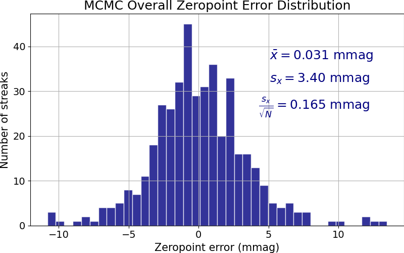
Figure 6: MCMC/PSF fitting zeropoint error distribution

Using MCMC photometry, we were consistently able to recover the image zeropoint accurately. Over 425 simulated streaks, the mean deviation of the results from the true zeropoint was only 0.0308mmag with a standard deviation of 3.41mmag. The standard deviation of the mean is therefore 0.165mmag, and we can therefore say with 99.7% (3$\sigma$) confidence that any systematic bias in these results owing to Streaktools has a magnitude of less than 0.5mmag under these (fairly typical) circumstances. Shown in figure 4 and 5 are the zeropoint error plotted against two measures of streak brightness; their intensity (in counts per unit length of the streak) and magnitude. The error bars are estimates of the uncertainty in the mean of the posterior distribution. As one might expect, zeropoint error is improved with more intense and overall brighter streaks, but this relationship is less strong than for pill photometry.

6 Discussion

Our results demonstrate a) that pill photometry applied to light streaks from LEO light sources cannot provide any passable or currently useful photometric calibration for modern science, but b) that MCMC/PSF fitting, as described here, could be plausibly used for very accurate photometric calibration that could be a useful and competitive complement or alternative to currently established, ground-based methods. Our 1$\sigma$ zeropoint error of 3.41mmag (flux error $\sim$0.3%) is comparable to what may be reached by contemporary ground-based photometry (Hartman et al., 2005; Stubbs & Tonry, 2006). To more conclusively demonstrate the potential of this approach for photometric calibration, more simulations, and especially calibrations using real orbital sources, will need to be performed. Streaktools can and should be tested in different circumstances. The accuracy provided by streaks which are comparatively very bright or dim could be interesting to investigate, in pursuit of maximum accuracy and the cost effectiveness of any orbital calibrator, respectively. In addition, we identify several nuances specific to light streak photometry. First, observations for light streak photometry should consist of minimally short exposures; only enough time to capture a full ‘pulse’ from a source. Extra exposure time beyond this will only add noise. Calibration sources should be engineered for short, bright pulses rather than longer and dimmer ones, since this would allow the exposure time to be brought down and increases streak intensity.

Conclusion

Here we have introduced and explored the concept and theoretical backing of light-streak photometric calibration using artificial light sources in LEO, and have introduced Streaktools, publicly available code with which to simulate light streaks and perform light streak photometry. Using Streaktools, we have shown pill photometry to be too inaccurate for precise calibration, but that MCMC-based maximum likelihood model fitting is able to provide an unbiased and accurate (1$\sigma$ error = 3.41mmag) estimate of the zeropoint of a real exposure, with streaks simulated using reasonable light source specifications. This suggests that photometric calibration using LEO sources has strong potential for use in precise photometric calibration, which should be explored.