Rankitect: Ranking Architecture Search Battling World-class Engineers at Meta Scale

Abstract.

Neural Architecture Search (NAS) has demonstrated its efficacy in computer vision and potential for ranking systems. However, prior work focused on academic problems, which are evaluated at small scale under well-controlled fixed baselines. In industry system, such as ranking system in Meta, it is unclear whether NAS algorithms from the literature can outperform production baselines because of: (1) scale – Meta’s ranking systems serve billions of users, (2) strong baselines – the baselines are production models optimized by hundreds to thousands of world-class engineers for years since the rise of deep learning, (3) dynamic baselines – engineers may have established new and stronger baselines during NAS search, and (4) efficiency – the search pipeline must yield results quickly in alignment with the productionization life cycle. In this paper, we present Rankitect, a NAS software framework for ranking systems at Meta. Rankitect seeks to build brand new architectures by composing low level building blocks from scratch. Rankitect implements and improves state-of-the-art (SOTA) NAS methods for comprehensive and fair comparison under the same search space, including sampling-based NAS, one-shot NAS, and Differentiable NAS (DNAS). We evaluate Rankitect by comparing to multiple production ranking models at Meta. We find that Rankitect can discover new models from scratch achieving competitive trade-off between Normalized Entropy loss and FLOPs. When utilizing search space designed by engineers, Rankitect can generate better models than engineers, achieving positive offline evaluation and online A/B test at Meta scale.

1. Introduction

Neural Architecture Search (NAS) seeks to automatically generate new architectures for deep learning models. A seminal work (Zoph and Le, 2016) proved the efficacy of NAS in the era of deep learning to design convolutional networks for computer vision and recurrent cells for natural language processing. It stimulated a line of academic research, typically in computer vision (Zoph et al., 2018; Wu et al., 2019; Tan and Le, 2019) and later in ranking systems (Zhang et al., 2023a; Gao et al., 2021; Krishna et al., 2021). One of the major research areas around NAS has been improving its computational efficiency, including more efficient sampling-based methods (Wen et al., 2020; Real et al., 2019; White et al., 2021; Fedorov et al., 2019), one-shot (Pham et al., 2018; Bender et al., 2020b) and DNAS (Xie et al., 2018; Liu et al., 2018; Fedorov et al., 2022; Banbury et al., 2021). However, those methods have never been evaluated at web-scale applications with billions of users for generating brand new ranking models from scratch by composing low-level building blocks. In this paper, we develop Rankitect, which advances NAS to Meta scale with comprehensive evaluation:

• Search space: Our search space includes almost no inductive bias from the production model. The discovered architecture is a mapping between feature embeddings and final classification layer. Building blocks are low-level operations like linear, dot product, etc. Connectivity among blocks is arbitrary. Block dimensions are searchable;

• Improved three categories of search algorithms: sampling-based methods (Wen et al., 2020; Zoph and Le, 2016) under different low cost proxies, one-shot method (Bender et al., 2020b) with in-place co-trained baseline model and DNAS (Xie et al., 2018);

• Baseline: the strongest production model at Meta, which is a Click Through Rate (CTR) model optimized by world-class engineers driven by years of business needs.

This industry level NAS at Rankitect scale imposes significant challenges and we advance current SOTA methods to succeed:

• Low cost evaluation analysis: for sampling-based methods, training a sampled model for long term is unrealistic, e.g. $>50$ billion examples at Meta scale. When a small amount of data is used, we compare the ranking quality between weight-sharing proxy (Bender et al., 2018) and early-stop proxy, and find weight-sharing proxy is superior when the data amount is small but will be surpassed by simple early-stop proxy when more data is used; based on our decision framework, early stop proxy is preferred in practice when requiring a higher ranking quality and more efficient engineering and system optimization.

• Noise reduction by an in-place baseline in one-shot method: data distribution of real-world ranking systems shifts dramatically, which makes the absolute metric – normalized entropy (NE) loss (He et al., 2014) – noisy over the training course. To cancel the noise introduced by data shifting, we co-train a baseline model in parallel with the weight sharing supernet in one-shot method (Bender et al., 2020b), and use the relative improvement of a model/subnet sampled from the supernet versus the baseline as the reward of the Reinforcement Learning (RL) agent;

• A joint on-policy/off-policy RL method to improve sample efficiency: RL based one-shot NAS suffers from costly reward evaluation and extreme sample inefficiency. To address both challenges, we propose a joint on-policy and off-policy policy gradient method that uses experience replay to amortize the computational cost of reward evaluation and improve sampling efficiency by decoupling RL policy updates from that of weight sharing supernet.

• DNAS: We implement differentiable NAS (DNAS) to optimize decision variables in conjunction with supernet weights. The DNAS approach exhibits increased efficiency compared to sampling-based methods and improves convergence characteristics compared to one-shot method using RL.

• System optimization: Optimizing NAS within expensive search spaces presents inherent computational challenges in production system. To overcome this challenge, we developed tailored techniques such as: (1) activation checkpointing; (2) employing system-wide vectorized operations; (3) utilizing transfer learning to facilitate supernet weight sharing; (4) Round-Robin process groups to mitigate AllReduce overhead; (5) dynamic execution of partial operators in PyTorch graphs. These strategies collectively enhance the efficiency and effectiveness of Rankitect search.

With improved NAS methods, we find that

• Rankitect can generate brand new ranking models from scratch and outperform production models. Three methods in Rankitect all generated models along the NE-FLOPs Pareto front, but one-shot and DNAS are about $145\times$ efficient in terms of GPU hours. While one-shot and DNAS are on-par in terms of model quality and search efficiency, we find one-shot method can be implemented more easily with higher memory efficiency.

• During the dynamic iteration of the production model, in-house world-class engineers were also able to invent models beating the baseline. When battling human models, Rankitect models can cover different regions along the Pareto frontier of NE-FLOPs. Moreover, by utilizing the human designed model as a search space, Rankitect produces models with NE-FLOPs trade-off better than engineers achieving positive offline evaluation and online A/B test at Meta scale.

2. Related Work

Neural Architecture Search (NAS) is a generic approach to design deep learning models in various applications, such as, computer vision (Pham et al., 2018; Bender et al., 2020b; Wen et al., 2020; Real et al., 2019; Wu et al., 2019; Tan and Le, 2019; Zoph et al., 2018; Zoph and Le, 2016; Bender et al., 2020a), natural language processing (Zoph and Le, 2016; Klyuchnikov et al., 2022; So et al., 2019) and speech (Mehrotra et al., 2020; Abdelfattah et al., 2021). Its adoption to ranking systems is also ramping up (Zhang et al., 2023a; Krishna et al., 2021; Gao et al., 2021; Song et al., 2020; Zhang et al., 2023b; Cao et al., 2023), however those work evaluated NAS with small public datasets using small search space. For example, the DNAS (for ads CTR prediction (Krishna et al., 2021)) and PROFIT (Gao et al., 2021) only search a portion of ranking models with a limited number of choice options. NASRec (Zhang et al., 2023a) scales the search space to a larger extent but the number of choices to select building blocks is just $7$. Unlike those work, Rankitect evaluates web-scale NAS at Meta scale with a much larger dataset ($>50$ billions of examples) and a much larger search space ($\geq 28$ choices of building blocks).

NAS has also been applied to industry level ranking systems (Liu et al., 2020; Li et al., 2023; Zhaok et al., 2021; Anil et al., 2022), however, the search space is relatively trivial: AutoFIS (Liu et al., 2020) uses DNAS like gates to select predefined feature interactions for Huawei App Store ranking systems; ByteDance proposed AutoEmb (Zhaok et al., 2021) to learn embedding dimensions, and Google’s H₂O-NAS (Li et al., 2023) is adopted to learn MLP sizes and embedding dimensions. None of them has studied the aggressive search space like Rankitect, which searches building block per layer, connections among blocks and dimensions per block, all at once..

Moreover, only one NAS algorithm was adopted in previous work, such as sampling-based methods in AutoCTR (Song et al., 2020) and NASRec (Zhang et al., 2023a), DNAS in AutoFIS and one-shot method in H₂O-NAS. This imposes challenges to understand the scalability and effectiveness of different NAS algorithms because the setups are different across different works/companies. Rankitect evaluates three categories of NAS algorithms (sampling-based methods, DNAS and one shot method) using the same dataset, search space, baseline and engineering constraint. This provides valuable insights to select appropriate NAS methods based on real-world conditions.

3. Method

In this section, we introduce the search space and three NAS algorithms we developed.

3.1. Search Space and Supernet Design

Search space is defined as the set of all possible models. In Rankitect, we bag all possible models into a single weight sharing supernet model (Bender et al., 2018) as detailed in Figure 1, and a model in the search space is produced by masking out connections & building blocks and selecting specific dimensions for building blocks. As a selected model is materialized as a sub-architecture of the supernet, we interchangeably use “subnet” and “model”.

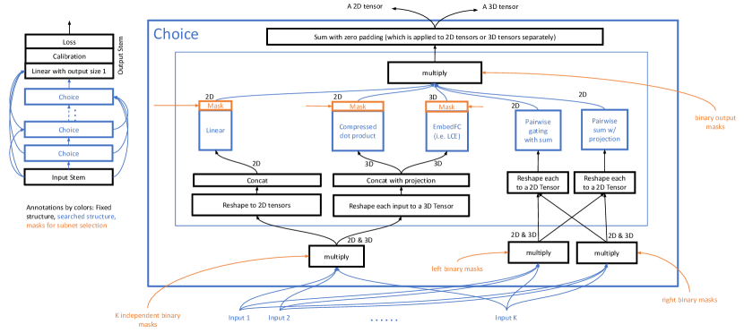
Figure 1. Search space in sampling-based methods and supernet in one-shot method and DNAS

Rankitect searches the end to end architecture between raw inputs (a dense feature 2D vector and a 3D embeddings concatenated from sparse/category embeddings and content embeddings) and the final logit used for CTR prediction. For simplicity, a 3D or 2D tensor is denoted as $X_{3d}\in\mathbb{R}^{B\times N\times D}$ or $X_{2d}\in\mathbb{R}^{B\times S}$, respectively. $B$ is batch size, $N$ is the number of embeddings, $D$ is embedding dimension, and $S$ is the size of a 2D vector. In Rankitect, all 3D tensors have the same embedding dimension $D$.

The supernet is constructed by stacking a cascade of “Choice” modules which can be fully densely connected to previous choices and raw inputs. All Choice modules have the same architecture which consists of three parts:

1. Input adaptors, which adapt inputs for valid computation of each building “block”. We have three types of adaptors as shown in Figure 1: (1) reshape each input to a 2D tensor and concatenate together before the linear block; (2) concatenate all inputs to a single 3D tensor along the middle axis (when an input is $X_{2d}\in\mathbb{R}^{B\times S}$, it is expanded to $X_{3d}\in\mathbb{R}^{B\times 1\times S}$ and then linearly projected to $X_{3d}\in\mathbb{R}^{B\times 1\times D}$ for concatenation with other 3D tensors). This adaptor is used before compressed dot product and EmbedFC blocks; (3) reshapes each input to a 2D tensor before pairwise gating and sum blocks.

2. Building blocks, which are layer types we want to search. Rankitect generates models from the elementary low level building blocks below:

   • linear or fully connected (FC) layer

   • EmbedFC is a linear projection applied to the middle axis of input $X_{3d}\in\mathbb{R}^{B\times N\times D}$ and produces $X_{3d}\in\mathbb{R}^{B\times M\times D}$, therefore, it is a linear with weight matrix $W\in\mathbb{R}^{M\times N}$;

   • compressed dot product is simply pairwise dot products among compressed embeddings and raw embeddings as

     (1) $$flatten\left(bmm\left(X_{3d},EmbedFC(X_{3d})^{T}\right)\right),$$

     where $bmm(\cdot)$ is batch matrix-matrix product ;

   • pairwise gating block has $K$ inputs $X_{2d}^{(i)}\in\mathbb{R}^{B\times S_{i}}$ where $i\in{1...K}$, it computes as

     (2) $$\sum_{i=1}^{K}\sum_{j=1}^{K}interaction\left(FC_{ij}\left(X_{2d}^{(i)}\right),X_{2d}^{(j)}\right),$$

     where $FC_{ij}(\cdot)$ projects $X_{2d}^{(i)}$ from dimension $S_{i}$ to $S_{j}$ and $interaction(x,y)=sigmoid(x)\circ y$ known as Hadamard product. $\sum_{i=1}^{K}\sum_{j=1}^{K}(\cdot)$ will zero pad smaller tensors to maximum size of $\{S_{i}|i\in{1...K}\}$ before sum;

   • pairwise sum block is very similar to pairwise gating block and the only difference is that $interaction(x,y)=x+y$.

   Note that firstly layer normalization and then activation functions are appended after each block.

3. Output aggregators, which reduce outputs from all building blocks. In Rankitect, all 2D block outputs are zero-padded to the same shape and then sum together to form a single 2D tensor. As only one block (EmbedFC) produces a 3D tensor, the 3D tensor is outputted alone from the choice module.

In the supernet as colored by orange in Figure 1, Rankitect samples masks to sample a subnet/model from the search space. A subnet is sampled by selecting a building block within each choice module, choice connections, and block dimensions:

• building block sampling: Rankitect selects one block within each choice module, which is accomplished by sampling an one-hot “binary output masks”.

• choice connection sampling: when linear, compressed dot product or EmbedFC block is selected, “K independent binary masks” (multi-hot masks) are sampled to select a portion as inputs; when pairwise gating or sum block is selected, an one-hot “left binary masks” and one-hot “right binary masks” are sampled to enable only one pair of “$interaction(\cdot)$” in Eq. (2).

• block dimension sampling: when a block is linear, compressed dot product or EmbedFC, output dimension of the linear projection inside the block will be sampled. This is achieved by multiplying linear outputs by a vector of binary masks. A mask vector is constrained to values with leading ones followed by zeros (e.g. $[1,1,1,0,0]$). The length of leading ones equals an selected output dimension.

Note that, Rankitect can enable the whole supernet by setting all masks values to ones. With our supernet design, Rankitect flexibly supports a variety of NAS algorithms:

• sampling-based algorithms: any black-box sampling algorithms (random, reinforcement learning (Zoph and Le, 2016), Bayesian optimizer (White et al., 2021) and neural predictor (Wen et al., 2020)) can be used to sample masks (in orange) to sample a subnet/model;

• one-shot method: an in-place RL agent is co-trained with the supernet, with the agent sampling masks;

• DNAS: masks are replaced by Gumbel-Softmax  (Jang et al., 2016) learned by architecture parameters.

3.2. NAS Algorithms

At Meta, we use Normalized Entropy (NE) (He et al., 2014) loss to evaluate the prediction performance of ranking systems. A smaller NE presents a better ranking model. We use “NE gain” over a baseline to measure improvement – a negative “NE gain” implies a improved prediction. In the following, we introduce how each NAS algorithm works in Rankitect and what improvement we have proposed.

3.2.1. Sampling-based method

Based on study in computer vision on NASBench-101 (Ying et al., 2019; Wen et al., 2020), Neural Predictor (Wen et al., 2020) is a more efficient sampling-based method than Regularized Evolution (Real et al., 2019) and Reinforcement Learning, we select Neural Predictor given it also has traits of full parallelism and friendly hyper-parameter tuning. Unlike original method which used a random sampler to pick top models by the predictor, we use a RL sampler to do so for faster convergence.

As discussed, it is unrealistic to do a full job training at Meta dataset scale after a subnet/model is sampled. We compared two types of low cost NE proxies:

• weight-sharing proxy which has two stages: supernet pretraining and subnet finetuning. In supernet pretraining, the whole supernet is first trained for $10\%$ data (by setting all masks to ones), followed by enabling subnet sampling with a proability of $0.75$ at each mini-batch. That is, in the later $90\%$ supernet pretraining, at each mini-batch, the supernet has $0.25$ probability to train all architectures and $0.75$ probability to only train a sub-architecture (subnet) by uniform random sampling of masks (in orange in Figure 1). In subnet finetuning, the Neural Predictor will first sample and fix masks to select a subnet, and then the specific subnet (with weights shared/transferred from corresponding parameters from supernet) is fine-tuned for a small amount of data to get the final weight-sharing proxy. Note that fine-tuned weights in a sampled subnet will not be updated to the supernet.

• early-stop proxy, which simply trains a standalone subnet/model from scratch for little data. For this proxy, the supernet is never instantiated or trained; only the sub-architecture of a sampled model is realized as a PyTorch model for more efficient training.

Note that for both NE proxies of a subnet, window NE averaged over the last $25\%$ training/fine-tuning data is used because it better correlates with long term NE which is more important for CTR models in real-world ranking systems.

3.2.2. One-shot NAS with Reinforcement Learning

Motivated by the TuNAS one-shot method (Bender et al., 2020a), we co-train an in-place RL agent with the supernet simultaneously illustrated in Figure 2. At each mini-batch, the RL agent samples masks to select a subnet and the mini-batch NE is used as reward to update the RL agent. More specific, we treat all the decisions (i.e., mask selections in the supernet) as independent multinomial random variables (r.v.). Let $\mathbf{\theta}$ be a vector (collection) of parameters that define all the decision’s multinomial r.v.. We use REINFORCE (Williams, 1992) to update the sampling distribution $P_{\mathbf{\theta}}$ with policy gradient:

(3) $$\nabla_{\mathbf{\theta}}\sum_{i}\log P_{\mathbf{\theta}}(a_{i})(R_{i}-b),$$

where $a_{i}$ is a sampled subnet and $R_{i}$ is the reward (e.g. NE and FLOPs) of $a_{i}$. A baseline function $b$ is used to reduce the variance of policy gradient and in our work we define $b$ to be the average over all $R_{i}$. In the following, we discuss technical challenges of this TuNAS-like one-shot method in Rankitect and our proposals to overcome them. We use “RL method” and “one-shot method” interchangeably in this paper.

Noisy reward and variance reduction

When applying RL to NAS for ranking problem, a main component of $R_{i}$ is the mini-batch NE, $NE_{batch}(a_{i})$. However, $NE_{batch}(a_{i})$ in production environment is: (1) extremely noisy (i.e., high variance) and (2) non-stationary caused by data distribution shift. To overcome these challenges, we borrow ideas from the control variate method where we subtract a correlated baseline reward, denoted as $NE_{batch}(baseline)$, from $NE_{batch}(a_{i})$. More specifically, we propose the following:

1. Calculate $NE_{batch}(baseline)$ from an in-place baseline model co-trained in parallel with the supernet.

2. Replace $NE_{batch}(a_{i})$ used in $R_{i}$ with $NE_{\%}(a_{i})$:

   (4) $$NE_{\%}(a_{i})=\frac{NE_{batch}(a_{i})-NE_{batch}(baseline)}{NE_{batch}(baseline)}$$

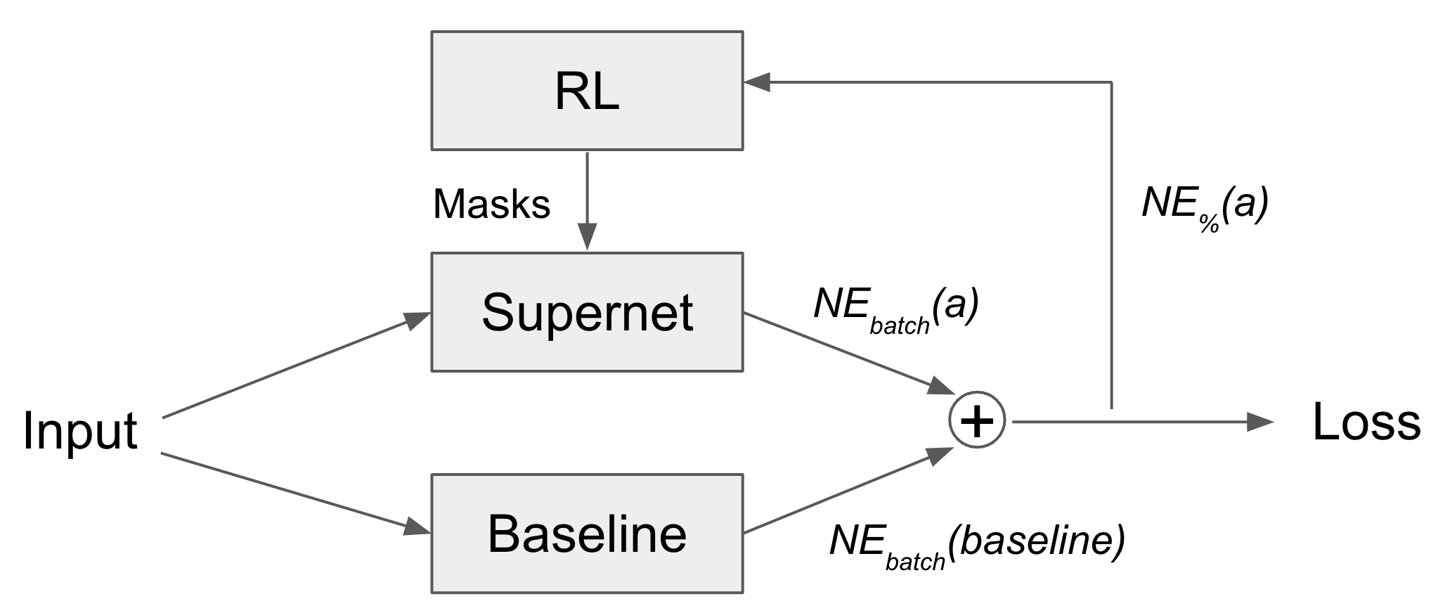
Figure 2. In-place training a baseline model with RL sampling subnets from the supernet.

Figure 2 illustrates how the proposed $NE_{batch}(baseline)$ and $NE_{\%}(a_{i})$ integrate with the weight sharing supernet training. A detailed ablation study for this part is included in Appendix A (see Figure 8 and 9)

Sample scarcity and on/off-policy RL

REINFORCE is an on-policy method where it can only learn through sampling from the current $P_{\mathbf{\theta}}$. This limitation introduces inefficiency in NAS for industry-scale ranking problems, because of:

1. costly reward evaluation: evaluating $R_{i}$ for an industry-scale model architecture is computationally expensive such that the number of samples is prohibited; and

2. extreme sampling inefficiency: RL policy’s updating schedule is slower than that of the supernet update (i.e., Eq. (3) requires a batch of model evaluations where each needs a mini-batch of subnet/supernet training). Consider an example of using batch size 100 for Eq. (3), then a supernet trained over one million steps (typical budget) only generates $10,000$ RL policy updates which is a challenge for on-policy RL algorithms.

To address these challenges we adopted off-policy RL methods reusing past samples $(a_{i},R_{i})$ for policy updates with experience replay (Mnih et al., 2013). This allows us to amortize the computational cost of reward evaluation and improves sample efficiency by decoupling policy updates from supernet updates. We followed a standard formulation of the off-policy policy gradient (PG) based on importance sampling (IS) (Mahmood and Sutton, 2015). A main challenge of off-policy implementation is controlling for the possible high variance (infinite variance in some cases) of the IS weights (a ratio of two probability functions). In this work, we adopted two techniques to mitigate the potential problem of high IS weights variance: (1) IS weights clipping; (2) weighted importance sampling (WIS) (Mahmood and Sutton, 2015; Schlegel et al., 2019; Metelli et al., 2020). In summary, we adopted the following policy gradient with off-policy IS:

(5) $$\nabla_{\mathbf{\theta}}\sum_{i}\frac{w_{i}}{\sum_{j}w_{j}} \log P_{\mathbf{\theta}}(a^{\prime}_{i})(R^{\prime}_{i}-b^{\prime}),\;\;(\mathbf{\theta}^{\prime}_{i},a^{\prime}_{i},R^{\prime}_{i})\sim B,$$

(6) $$w_{i} =\min\left[\frac{P_{\mathbf{\theta}}(a^{\prime}_{i})}{P_{\mathbf{\theta}^{\prime}_{i}}(a^{\prime}_{i})+\epsilon},1e4\right].$$

where $\epsilon$ is a small number to avoid divide-by-zero, $w_{i}$ is the WIS weights, $b^{\prime}$ is the average over all $R^{\prime}_{i}$, and $(\mathbf{\theta}^{\prime}_{i},a^{\prime}_{i},R^{\prime}_{i})$ is a random sample drawn from a replay buffer $B$ that stores past samples. Note that we also store the multinomial r.v. parameter $\mathbf{\theta}^{\prime}$ that are used to sample $a^{\prime}_{i}$. Since RL policy is trained concurrently with the supernet, recent $(a^{\prime}_{i},R^{\prime}_{i})$ samples are more relevant/accurate than older samples. Based on this observation, we propose a joint on-policy and off-policy PG (denoted as on/off-policy PG) where we first perform on-policy update using Eq. (3) (and store new batch of $(\mathbf{\theta}^{\prime}_{i},a^{\prime}_{i},R^{\prime}_{i})$ to $B$) followed by $K$ off-policy updates using Eq. (5). We also experimented with prioritized experience replay (Schaul et al., 2016) but found our proposal that guarantee on-policy update at each step to perform better in practice . With the proposed on/off-policy method, we can achieve a $K\times$ increase in the number of policy updates compared to on-policy REINFORCE. A detailed ablation study for this part is included in Appendix (see Figure 10).

NE search with FLOPs constraint

To promote the discovering of models with good NE and FLOPs trade-off, we augment reward function with an additive cost term:

(7) $$R_{i}=NE_{\%}(a_{i})+\alpha\cdot Cost(a_{i}),$$

where $\alpha$ is a regularization weight that balances the trade-off between NE and FLOPs. For $Cost(a_{i})$, we experimented with L1-penalty $\|FLOPs(a_{i})-c\|$ and ReLU-penalty $\max(FLOPs(a_{i})-c,\;0)$, where $c$ is the target FLOPs. From our experiment, we observe that using ReLU-penalty often leads to a model with smaller FLOPs and worse NE compared to using using L1-penalty. Our hypothesis is that the L1-penalty can better guide RL search during initial exploration towards the targeted FLOPs (penalize both above and below target FLOPs) and later lead to the convergence of a better local optimum model.

3.2.3. DNAS

We implemented DNAS (Liu et al., 2018; Cai et al., 2018; Dong and Yang, 2019) as an alternative to one-shot method for comprehensive study. DNAS directly optimizes the pair $(W,\theta)$:

(8) $$\min_{W,\theta:FLOPs(\gamma(\theta))\leq c}E_{a,d}\left[CE(W,a,d)\right]$$

where $\gamma(\theta)$ denotes the most likely subnet given $\theta$, $d$ is a batch of data, and $CE$ is the cross-entropy loss. The fundamental difference between RL and DNAS is in how we deal with the non-differentiable expectation over $a$ in (8). Each of the decisions of $a$ is a categorical r.v., such that differentiation of (8) is not possible. In DNAS, the categorical r.v.’s are replaced by Gumbel-Softmax r.v.’s, which lend themselves to the reparameterization trick for differentiation (Kingma and Welling, 2022; Fedorov et al., 2019; Krishna et al., 2021). The expectation in (8) is approximated using Monte-Carlo sampling, with each trainer and each minibatch element using a separate realization of $a$. In order to enforce the constraint in (8), we follow (Fedorov et al., 2022) and transform (8) into a regularized objective with a regularizer whose minimizer is guaranteed to satisfy the constraint:

(9) $$R=E_{a}\left[\left|FLOPs(a)-c\right|\right]$$

4. Experiments

In this section, we provide experimental results for end-to-end Rankitect search and compare the discovered model to strong production baselines created by ML experts. Three categories of algorithms are also compared.

4.1. Experiment Setup

We use industrial ranking systems’ datasets at Meta for all experiments. Input features include floating-point dense features, content embeddings, and sparse embeddings from categorical lookup tables. All embeddings are concatenated to a single 3D tensor. Click Through Rate (CTR) and Conversion Rate (CVR) models are evaluated, which are binary classifiers. Binary cross entropy loss is used for optimization, and we report Normalized Entropy (He et al., 2014) (NE). NE is simply normalized cross entropy which is less noisy over data distributions. A typical ranking model is trained by more than $50$ billion examples with Adam optimizer. All Rankitect searches are performed in GPU (up to 128) training cluster. During supernet search, PyTorch dynamic computation graphs are not well-suited for conventional optimizations. To streamline this process, we have explored and implemented several techniques, including activation check-pointing for reduced memory, employing vectorized operations to expedite computations, utilizing partial parameter transfer from the supernet to standalone subnets to efficiently obtain weight-sharing proxy, and implementing Round-Robin process groups to mitigate All-Reduce overhead (Li et al., 2020).

4.2. Full Architecture Search from Scratch Battling World-class Engineers

4.2.1. Supernet Design

To study the scalability of Rankitect, this section performs NAS in a search space as large as possible, using the largest and strongest CTR model baseline (dubbed as “CTR app 1”) at Meta. If we naively use all blocks within each choice and fully connect them, the supernet size explodes easily. For example, a single full choice already has $>8.5$ billion dense parameters, major contributors of which are pairwise gating and sum blocks. To reduce supernet size, we propose two optimizations:

• Sharing pairwise linear projections $FC_{ij}(\cdot)$ in Eq. (2): when the same pairwise interaction (gating or sum) appears in different choices, the interaction is computed once and shared;

• bottleneck layers in pairwise linear projections: $FC_{ij}(\cdot)$ in Eq. (2) is decomposed to two linear layers with a bottleneck dimension $256$ at the middle.

This gives supernet better scalability, however the number of choices we can scale is still prohibited when the supernet has full connections among all choices with each choice having all blocks. We constrain the connections and possible blocks per choice as below and reach a supernet with around one billion dense parameters.

We start from a supernet with an architecture matching our current production model (which is a model variant of DLRM (Naumov et al., 2019)), where each choice only has one building block to match a layer. We then grow the supernet as following steps:

• randomly permute the list of choices while keeping its directed acyclic graph (DAG) order, i.e., predecessors of a node always have smaller indices in the permuted list. This removes the layer order bias encoded by engineers;

• copy any choice having EmbedFC or compressed dot product block, and then insert it right after;

• in any choice, if any of [compressed dot product, EmbedFC] block exists, add the other; if any of [linear, pairwise gating, pairwise sum] block exists, add the others;

• each choice is connected to previous choices with distances of 1, 2, 3, 6 and 9, where “distance” is defined as the relative index of two choices in the choice list;

• enlarge linear dimensions in all blocks to $1.25\times$. There are $7$ dimension options uniformly distributed between $0.5\times$ and $1.25\times$.

The search space consists of $2.8\times 10^{114}$ models, which is $4.3\times 10^{95}$ times larger than the search space size in a typical computer vision problem (Wen et al., 2020) and $5.6\times 10^{78}$ times larger than a ranking systems NAS work in academia (Zhang et al., 2023a). The number of models is more than the number of atoms in the observable universe .

After finalizing the supernet, we tune the sampling probability of “K independent binary masks” in Figure 1 such that the distribution of subnets are reasonable. With probability $0.8$ to set a binary mask to one, Figure 3 plots the histogram of statistics of $10,000$ random subnets, where we can see that distributions spread well around our production model. Note that the production model is $5\times$ in terms of FLOPs, which is indicated by vertical dashed lines in Figure 3.

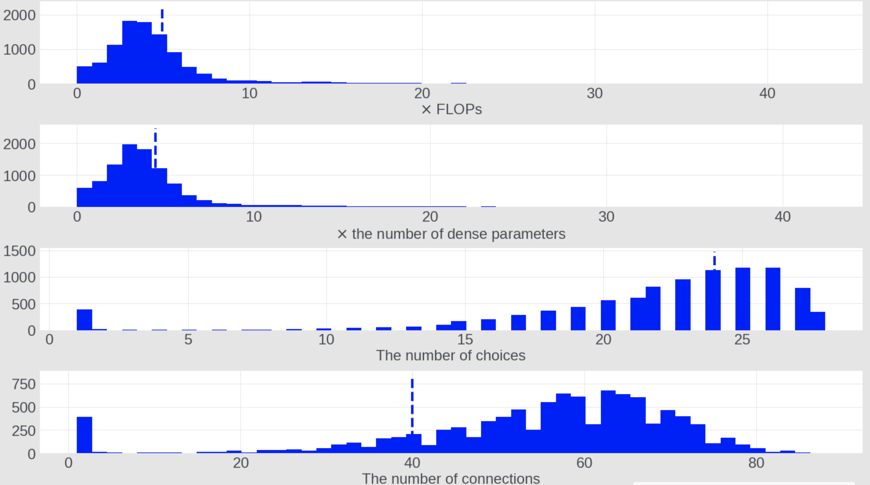
Figure 3. The distribution of FLOPs, # dense parameters, # choices and # connections in subnets. Vertical dashed lines are for the production model.

4.2.2. Weight-Sharing Proxy and Early-Stop Proxy

To evaluate which low cost NE proxy is better under specific conditions, we randomly sample $60$ models and train each from scratch for $28$B examples (“B” is for “billion”) to get long term NE. The window NE averaged on last $0.5$B examples is used as ground truth long term NE. Figure 4 plots the Kendall Tau rank correlation between proxies and ground truth NE. We find that weight-sharing NE has better correlation quality initially to rank ground truth NE, however, its advantage disappears when the amount of data passes a threshold ($200$ million in our search space). This is reasonable because weights used in weight-sharing proxy have been pre-trained in the supernet, such that a subnet does not need to train from scratch and therefore outperforms when the training data is less; however, as data amount increases, early-stop proxy approaches to ground truth NE but weight-sharing proxy may have inferior initialization for any subnet to achieve so.

In conclusion, weight-sharing proxy should be used if speedy subnet evaluation is required and a moderate rank quality (e.g. Kendall Tau $0.6$) satisfies; however, early-stop proxy should be used if a high rank correlation is demanded. Moreover, engineering and machine learning system optimization overheads should also be considered in practice, such as, in weight-sharing proxy, it is non-trivial to implement partial weight transfer from the supernet to any standalone subnet. In our experiments, we find high rank correlation is important to search models with long term NE, and decided to use early-stop proxy with $3$B training data, which has around $0.8$ Kendall Tau ranking quality.

Figure 4. Rank correlation between low cost proxies and long term ground truth NE, which is obtained by training for $28$B examples. Vertical intervals are confidence intervals from $25\%$ to $75\%$ quantile. Right figure just zooms into the beginning parts of curves on the left.

4.2.3. Results of Sampling-based Method

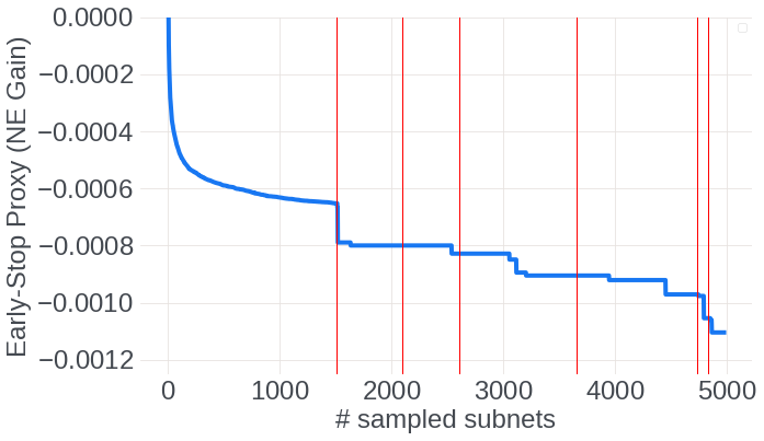
(a)

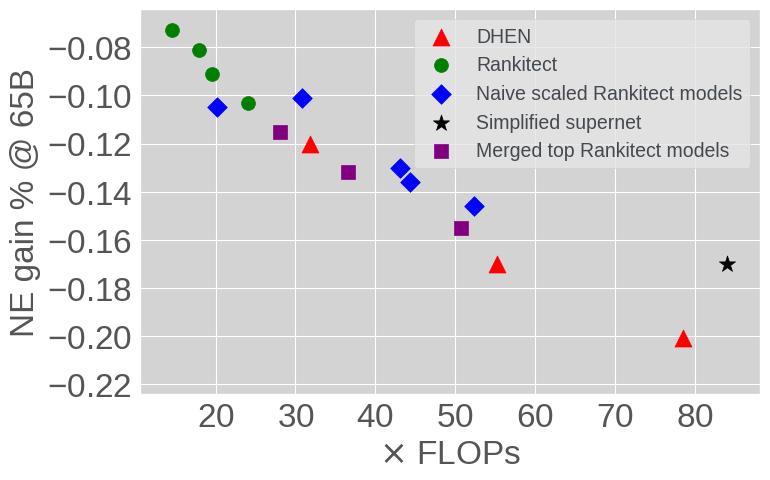
(b)

Figure 5. Results of Sampling-based Method: (a) NE gain of early-stop proxy. The vertical red lines divide different rounds of sampling-based search. The first round is random search (whose curve is smoothed by averaging over $500$ random permutations), followed by six rounds of Neural Predictor based sampling. For each new round, a MLP is trained by using all previously obtained data points and then picks top models based on MLP prediction; (b) long term NE gain at $65$ billion data examples versus production model.

We applied sampling-based method to search models for low early-stop proxy (which is better if lower). Figure 5(a) is the minimal early-stop NE found as more and more models are sampled and evaluated. In experiments, Neural Predictor bent the curve after initial random sampling. In total, we sampled $5,000$ models. As low early-stop proxy does not guarantee long term NE, we picked $100$ models with lowest early-stop NE and trained for more data with Successive Halving (Jamieson and Talwalkar, 2016), ending up with final $4$ best models plotted as green cycles in Figure 5(b).

In Figure 5(b), we can find that Rankitect can discover a new model with $0.10\%$ absolute NE gain which is considered as significant in ranking systems. Moreover, discovered models cover a good range of model complexity (FLOPs) from $14.5\times$ to $24\times$, which provides a good pool of models to select from for different serving cost constraints required by different products and model types. During Rankitect development, in-house engineers also invented a new model – DHEN (Zhang et al., 2022) as plotted in red triangles. Battling with Rankitect, DHEN covers a new region – more NE gain with more FLOPs. The combination of Rankitect and DHEN covers a wider range of FLOPs for different products’ serving cost requirements. To compare with DHEN in the high-FLOPs region, we propose two methods to scale Rankitect models:

• Naive scaling (blue diamonds): $3\times$ linear dimension in EmbedFC (first blue diamond from the left), OR, simultaneously $1.5\times$ linear dimensions in [linear, EmbedFC and compressed dot product] blocks and $2\times$ bottleneck dimensions in pairwise gating and sum blocks;

• Merging (purple squares): pick a subset of Rankitect models (green circles), for a connection or a block existing in any Rankitect model, add it to the final merged model. For a block having different linear dimensions in different Rankitect models, use the maximal dimension in the final merged model.

In Figure 5(b), we find the “Merging” method has a better NE-FLOPs trade-off than “Naive scaling”. Battling with DHEN, scaled Rankitect models have on-par NE-FLOPs trade-off trend, but fills the big blank FLOPs region which DHEN is unable to cover. Moreover, Rankitect automates the process of new architecture design, which can release human engineering resources.

Table 1. Rankitect search summary for DHEN-based supernet.

Model	Product applying Rankitect	DHEN layers / # decisions / search space	Supernet FLOPs	$\alpha$	Discovered FLOPs	Search cost1 (GPU hours)
1	CTR app 1	4 / 93 / $9^{93}$	80$\times$	2e-5	31.2$\times$	6144
2	CTR app 1	2 / 28 / $9^{28}$	10$\times$	1e-3	2.6$\times$	3072
3	CTR app 1	2 / 28 / $9^{28}$	2.65$\times$	2e-3	0.6$\times$	3072
4	CTR app 1	1 / 19 / $9^{19}$	1.08$\times$	1e-2	0.37$\times$	1536
1. all searches ran with 64 GPUs and the search cost are reported in total GPU-hours, e.g., 6144 GPU-hour = 64 GPU * 96 wall-clock hour.

4.2.4. Results by One-shot Method and DNAS

In our experiments, we find that it is challenging for one-shot method and DNAS to learn connections in the supernet designed in Section 4.2.1, therefore, we simplified the supernet by disallowing adding new connections and only learn to select a building block per choice. The NE gain and FLOPs of the simplified supernet is plotted as the black star in Figure 5(b). Our goal in this section is to answer the following questions:

• Does one-shot method or DNAS produce better NE models than sampling-based method?

• How do the search costs of three categories of methods compare?

• Is DNAS able to leverage the reduced variance of the Gumbel-Softmax gradient estimator compared to RL’s policy gradient (in one-shot method) to converge to solutions which satisfy a FLOPs constraint faster?

Figure 6 shows that the DNAS is able to find models which outperform the production model and sampling-based model, albeit at higher FLOPs cost. When we looked at the efficiency/cost of each method, DNAS and RL yield results with roughly $145\times$ less compute resources ($1.45$ days vs. $209.5$ days used by sampling-based method on 64 GPU system), which is a huge benefit at Meta-scale recommendation system training. Finally, we compare DNAS to RL and evaluate the effect of gradient variance on convergence performance since one of the benefits of DNAS is the reduced gradient variance compared to RL (Jang et al., 2016). We setup an experiment where both DNAS and RL try to search for a model with a target FLOPs (without considering its NE) and report that DNAS requires $\sim 26\times$ less SGD steps to converge to a given FLOPs target.

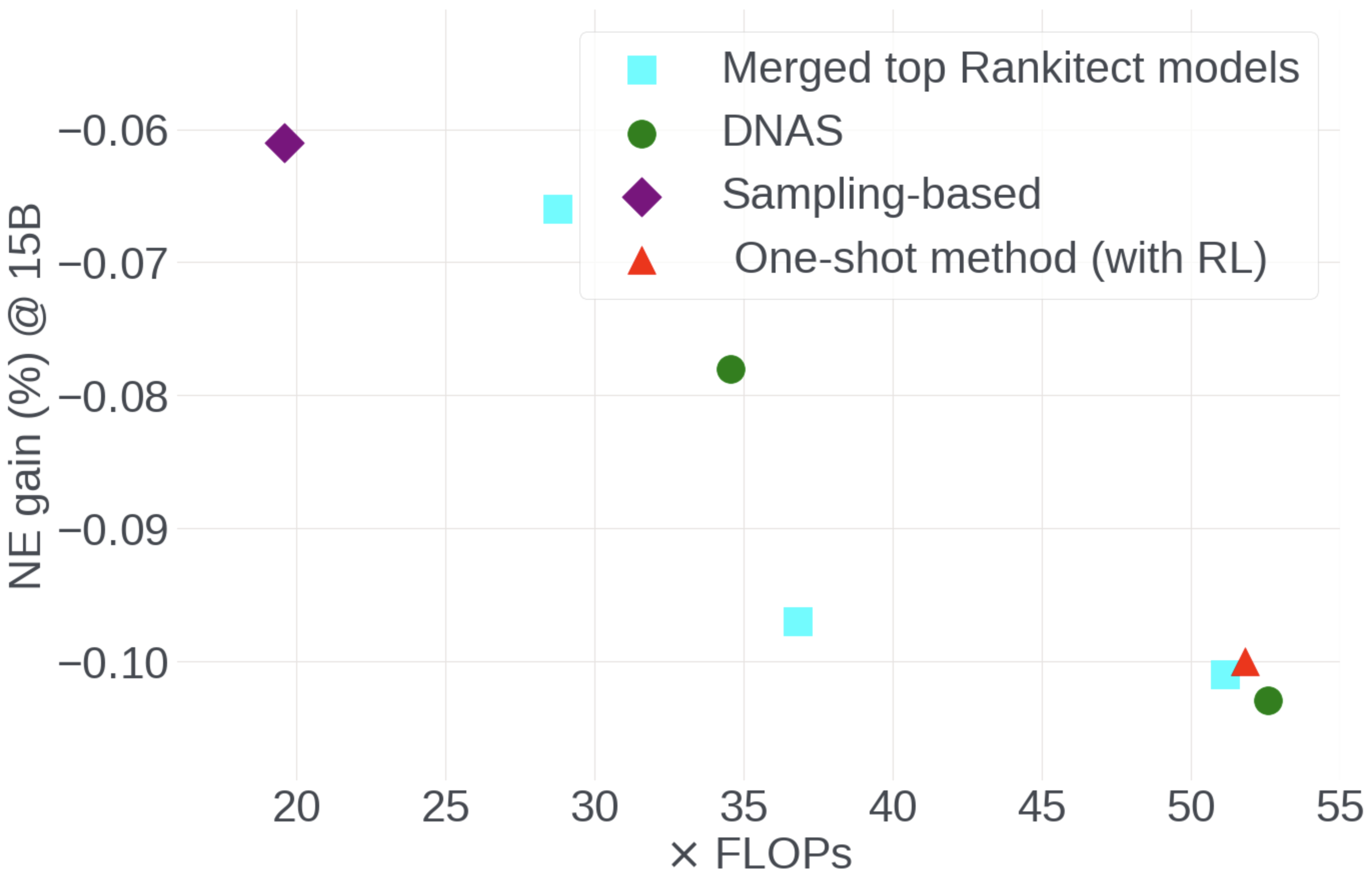
Figure 6. NE and FLOPs comparison of three categories of methods.

Although DNAS has overall the best performance, in the end we chose to focus our software system on RL instead of DNAS for the following reasons:

• The engineering cost of maintaining two search algorithms with relatively similar search performance is too high.

• Memory consumption of naive DNAS implementation is higher, demanding potentially more memory optimization overhead.

• The engineering cost of DNAS is higher than RL. DNAS requires careful tuning of hyperparameters like Gumbel-Softmax temperature, sparsity level of sampled r.v’s, etc. (Fedorov et al., 2022). Since the loss function is required to be differentiable for DNAS, optimization of FLOPs requires us to build a software library modeling FLOPs as a differentiable function of architecture. While this is possible, the engineering cost of building and maintaining such a library are quite high. On the other hand, RL can natively optimize non-differentiable objectives.

4.3. Reusing Search Space Invented by World-class Engineers

As proved in Section 4.2, Rankitect automatically produces competitive models versus world-class engineers with more diverse FLOPs coverage. More importantly, the result is generated from an unspecified supernet (or search space) with minor human prior. To bring the advantages from both worlds (of Rankitect and in-house engineers) together, we use DHEN as supernet backbone and apply Rankitect. We hypothesize that: human crafted DHEN-based supernet has a higher density of good models than the unspecified supernet, which makes Rankitect easier to find better models and can outperform human experts. We prove so in this section.

We setup a supernet to match the architecture of Deep and Hierarchical Ensemble Networks (DHEN) (Zhang et al., 2022) and focus on searching for all building block dimensions. For example, a $4$ layer DHEN-based supernet has $93$ building block dimensions to search; with each block dimension having 9 options, we have a search space with size $9^{93}$. The primary motivation for us to only search for block dimensions is to ensure an easy transfer of Rankitect search results to DHEN models in Meta’s production stack. To test the transferability, Rankitect is only applied on the strongest baseline at Meta for the “CTR app 1” product, and we simply apply the discovered models to other products. To meet different serving cost constraints of different products, we applied our Rankitect framework to various DHEN-based supernets, targeting different FLOPs goals. We summarize our search results in Table 1.

Beating strongest human baseline

During model iteration of “CTR app 1”, our in-house engineers were targeting on an approximately $30\times$ model for product and established the largest and strongest CTR baseline at Meta. To battle human engineers, Rankitect generated “model-1” in Table 1 which is a $31.2\times$ model with $>0.02\%$ absolute NE gain at $90$B (with gain still enlarging with more training data shown in Figure 7 in Appendix) compared with the human tuned $31.3\times$ baseline model. This proves that Rankitect can discover better models than Meta’s world-class engineers.

Table 2. Comparison of Rankitect and sampling-based production AutoML searcher.

Method	Model size	NE gain	Search cost (GPU-hour)
Rankitect	2.6$\times$	-0.28%	3072
Production AutoML	3.14$\times$	-0.35%	25600

Beating AutoML in production

We applied “model 2” to product “CVR app 0” and conducted a side-by-side comparison with a model discovered by sampling-based AutoML in production shown in Table 2. It turns out that our Rankitect model was able to meet FLOPs constraint for this product with significant NE gain, while production AutoML was not able to satisfy the FLOPs constraint. Furthermore, Rankitect achieved $8.3\times$ search efficiency gain over production AutoML (measured by GPU hours). Due to those, “model 2” was selected for online A/B test and show statistically significant gain over production model.

Strong model transferability to other products

We applied “Model 3” and “Model 4” across different products and observe strong model transferability. The results are summarized in Table LABEL:table:smt where we can see that “Model 3” is a smaller model but still achieve better NE performance in many of the products. On the other hand, “Model 4” achieve significant NE-gain over product baselines at the cost of model size increase. These results demonstrate that Rankitect has the potential to search once and apply to many.

Table 3. Transferability of Rankitect discovered models.

Model	Products	NE gain	FLOPs
3	CVR app 1	-0.053%	-34.5%
3	CVR app 2	0.04%	-40%
3	CVR app 3	-0.099%	-31.5%
4	CVR app 1	-0.173%	+20%
4	CVR app 2	-0.25%	+7%
4	CVR app 3	-0.254%	+23%

Appendix

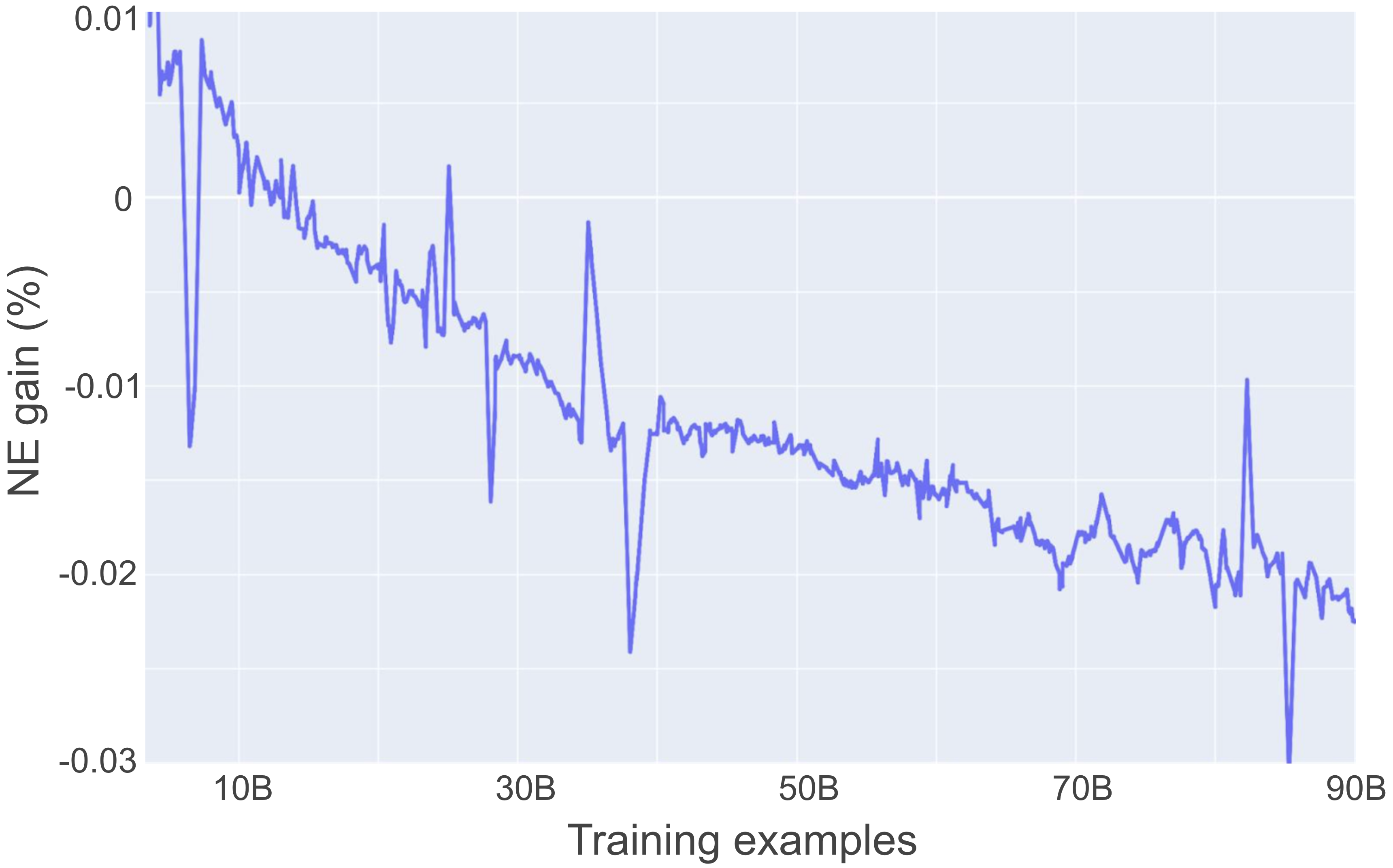
Figure 7. Offline training NE-gain of “model 1” compared against a 31.3$\times$ model tuned by strong human.

A. Ablation study of RL efficient search

In Section 3.2.2 we proposed $NE_{\%}(a_{i})$ to reduce noise by an in-place baseline in one-shot method and proposed an on/off-policy PG method to improve RL one-shot NAS sample efficiency. To validate the effectiveness of our proposals we present a detailed ablation study. First, we plot the observed $NE_{batch}(a_{i})$ and $NE_{\%}(a_{i})$ during a supernet training in Figure 8 where we can see that $NE_{\%}(a_{i})$ has significantly smaller variance compared to $NE_{batch}(a_{i})$. Next, we verify that using the less noisy $NE_{\%}(a_{i})$ as RL rewards also lead to improved Rankitect RL search. Figure 9 shows the NE gain of supernet when using $NE_{\%}(a_{i})$ as RL reward versus using $NE_{batch}(a_{i})$; a negative value indicates that Rankitect with $NE_{\%}(a_{i})$ reward consistently samples models with better NE performance than when using $NE_{batch}(a_{i})$ as reward (note that Figure 9 only optimizes for NE, i.e., $\alpha=0$).

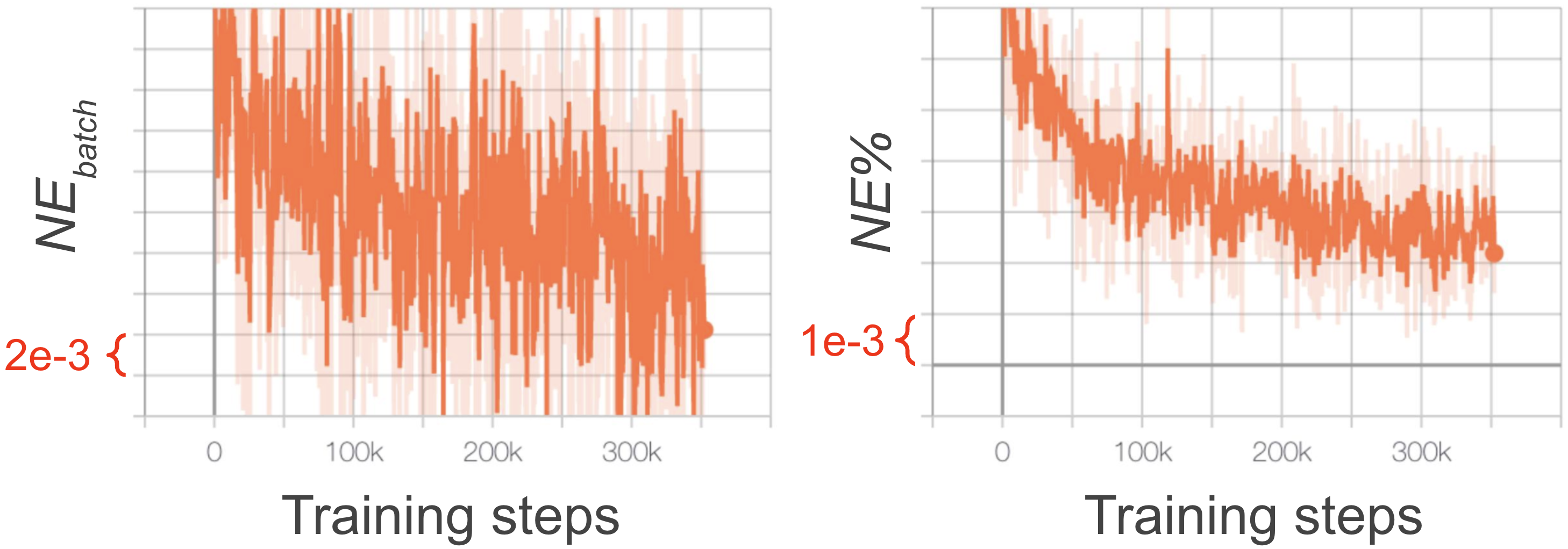
Figure 8. Observed NE signal during supernet training (left: $NE_{batch}(a_{i})$, right: $NE_{\%}(a_{i})$)

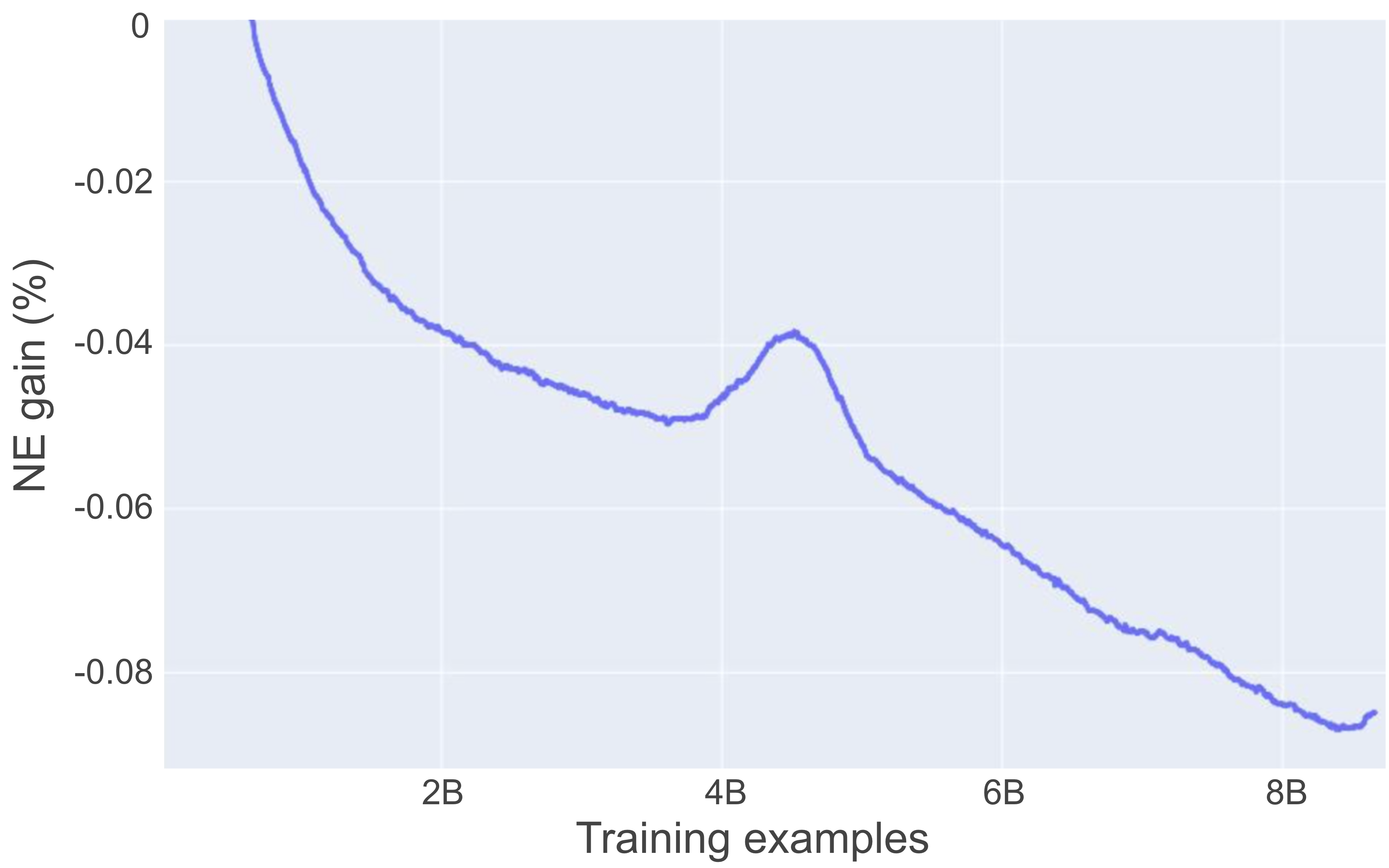
Figure 9. Supernet NE gain of using $NE_{\%}(a_{i})$ and $NE_{batch}(a_{i})$ as reward

Since computing $NE_{\%}(a_{i})$ (Eq. (4)) requires additional in-place training a baseline model, a natural question to ask is how does this affects Rankitect training/searching efficiency? We found that using $NE_{\%}(a_{i})$ as reward does not adversely affect search efficiency (compared to $NE_{batch}(a_{i})$); our speculation is that the training cost of the baseline model is negligible compared to the much larger supernet training cost.

To validate the effectiveness of the proposed on/off-policy PG method, we plot the RL reward convergence of REINFORCE and on/off-policy PG in Figure 10. From Figure 10 we can see that on/off-policy PG achieves faster learning . Moreover, we found similar search efficiency despite on/off-policy method receives 50$\times$ more policy updates than on-policy REINFORCE. Our speculation is that the computation cost of RL policy update is negligible compared to the much higher supernet training cost.

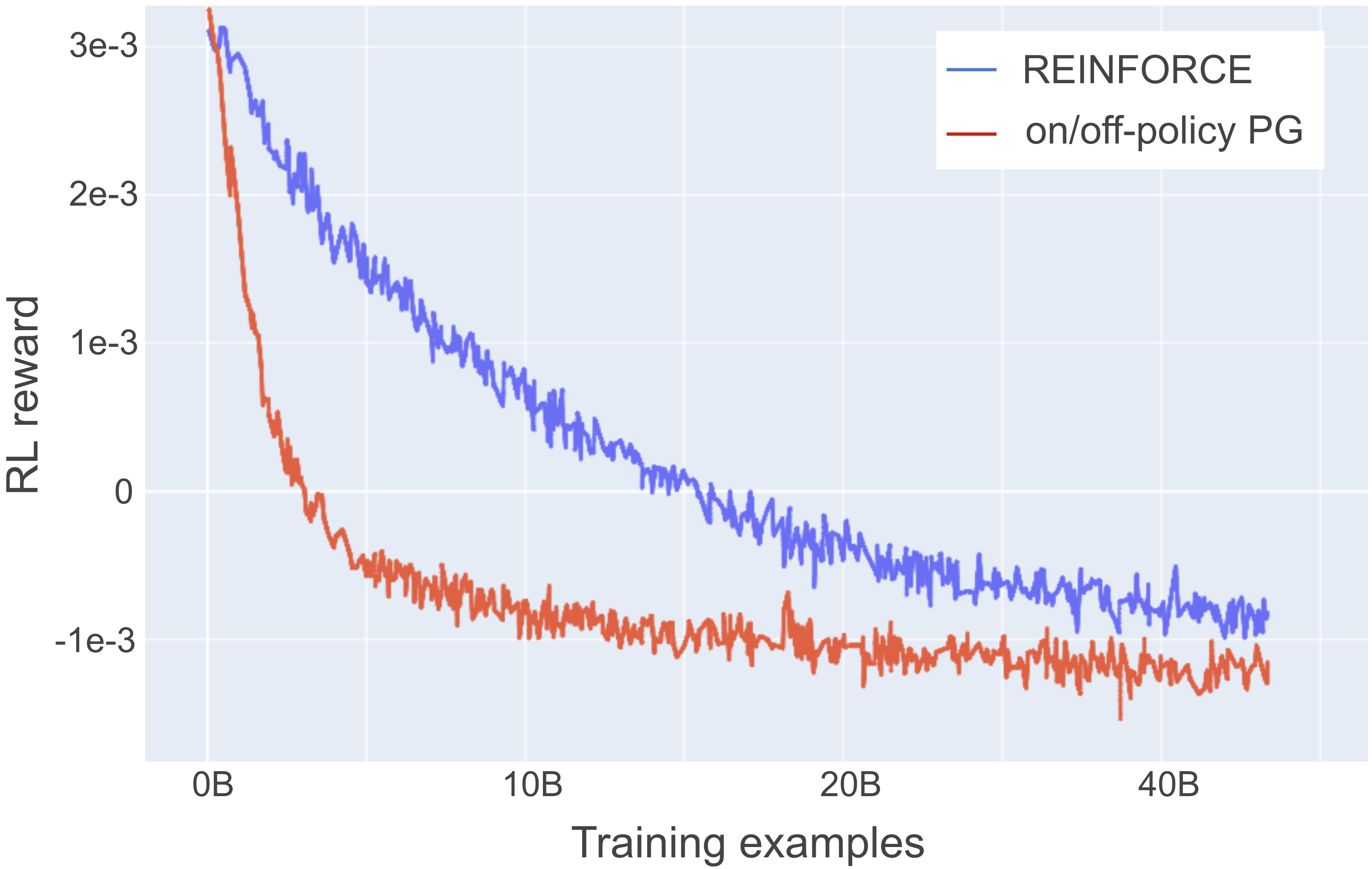
Figure 10. RL training comparison (red: on/off-policy PG, blue: on-policy REINFORCE)

References

- (1)
- Abdelfattah et al. (2021) Mohamed S Abdelfattah, Abhinav Mehrotra, Łukasz Dudziak, and Nicholas D Lane. 2021. Zero-cost proxies for lightweight nas. arXiv preprint arXiv:2101.08134 (2021).
- Anil et al. (2022) Rohan Anil, Sandra Gadanho, Da Huang, Nijith Jacob, Zhuoshu Li, Dong Lin, Todd Phillips, Cristina Pop, Kevin Regan, Gil I Shamir, et al. 2022. On the factory floor: ML engineering for industrial-scale ads recommendation models. arXiv preprint arXiv:2209.05310 (2022).
- Banbury et al. (2021) Colby Banbury, Chuteng Zhou, Igor Fedorov, Ramon Matas, Urmish Thakker, Dibakar Gope, Vijay Janapa Reddi, Matthew Mattina, and Paul Whatmough. 2021. MicroNets: Neural Network Architectures for Deploying TinyML Applications on Commodity Microcontrollers. In Proceedings of Machine Learning and Systems, A. Smola, A. Dimakis, and I. Stoica (Eds.), Vol. 3. 517–532. https://proceedings.mlsys.org/paper_files/paper/2021/file/c4d41d9619462c534b7b61d1f772385e-Paper.pdf
- Bender et al. (2018) Gabriel Bender, Pieter-Jan Kindermans, Barret Zoph, Vijay Vasudevan, and Quoc Le. 2018. Understanding and simplifying one-shot architecture search. In International conference on machine learning. PMLR, 550–559.
- Bender et al. (2020a) G. Bender, H. Liu, B. Chen, G. Chu, S. Cheng, P. Kindermans, and Q. V. Le. 2020a. Can Weight Sharing Outperform Random Architecture Search? An Investigation With TuNAS. In 2020 IEEE/CVF Conference on Computer Vision and Pattern Recognition (CVPR). IEEE Computer Society, Los Alamitos, CA, USA, 14311–14320. https://doi.org/10.1109/CVPR42600.2020.01433
- Bender et al. (2020b) Gabriel Bender, Hanxiao Liu, Bo Chen, Grace Chu, Shuyang Cheng, Pieter-Jan Kindermans, and Quoc V Le. 2020b. Can weight sharing outperform random architecture search? an investigation with tunas. In Proceedings of the IEEE/CVF Conference on Computer Vision and Pattern Recognition. 14323–14332.
- Cai et al. (2018) Han Cai, Ligeng Zhu, and Song Han. 2018. ProxylessNAS: Direct Neural Architecture Search on Target Task and Hardware. In International Conference on Learning Representations.
- Cao et al. (2023) Yufan Cao, Tunhou Zhang, Wei Wen, Feng Yan, Hai Li, and Yiran Chen. 2023. Farthest Greedy Path Sampling for Two-shot Recommender Search. arXiv preprint arXiv:2310.20705 (2023).
- Dong and Yang (2019) Xuanyi Dong and Yi Yang. 2019. Searching for a Robust Neural Architecture in Four GPU Hours. In Proceedings of the IEEE/CVF Conference on Computer Vision and Pattern Recognition (CVPR).
- Fedorov et al. (2019) Igor Fedorov, Ryan P Adams, Matthew Mattina, and Paul Whatmough. 2019. SpArSe: Sparse Architecture Search for CNNs on Resource-Constrained Microcontrollers. In Advances in Neural Information Processing Systems, H. Wallach, H. Larochelle, A. Beygelzimer, F. d'Alché-Buc, E. Fox, and R. Garnett (Eds.), Vol. 32. Curran Associates, Inc. https://proceedings.neurips.cc/paper_files/paper/2019/file/044a23cadb567653eb51d4eb40acaa88-Paper.pdf
- Fedorov et al. (2022) Igor Fedorov, Ramon Matas, Hokchhay Tann, Chuteng Zhou, Matthew Mattina, and Paul Whatmough. 2022. UDC: Unified DNAS for Compressible TinyML Models for Neural Processing Units. In Advances in Neural Information Processing Systems, S. Koyejo, S. Mohamed, A. Agarwal, D. Belgrave, K. Cho, and A. Oh (Eds.), Vol. 35. Curran Associates, Inc., 18456–18471. https://proceedings.neurips.cc/paper_files/paper/2022/file/753d9584b57ba01a10482f1ea7734a89-Paper-Conference.pdf
- Gao et al. (2021) Chen Gao, Yinfeng Li, Quanming Yao, Depeng Jin, and Yong Li. 2021. Progressive feature interaction search for deep sparse network. Advances in Neural Information Processing Systems 34 (2021), 392–403.
- He et al. (2014) Xinran He, Junfeng Pan, Ou Jin, Tianbing Xu, Bo Liu, Tao Xu, Yanxin Shi, Antoine Atallah, Ralf Herbrich, Stuart Bowers, et al. 2014. Practical lessons from predicting clicks on ads at facebook. In Proceedings of the eighth international workshop on data mining for online advertising. 1–9.
- Jamieson and Talwalkar (2016) Kevin Jamieson and Ameet Talwalkar. 2016. Non-stochastic best arm identification and hyperparameter optimization. In Artificial intelligence and statistics. PMLR, 240–248.
- Jang et al. (2016) Eric Jang, Shixiang Gu, and Ben Poole. 2016. Categorical Reparameterization with Gumbel-Softmax. In International Conference on Learning Representations.
- Kingma and Welling (2022) Diederik P Kingma and Max Welling. 2022. Auto-Encoding Variational Bayes. arXiv:1312.6114 [stat.ML]
- Klyuchnikov et al. (2022) Nikita Klyuchnikov, Ilya Trofimov, Ekaterina Artemova, Mikhail Salnikov, Maxim Fedorov, Alexander Filippov, and Evgeny Burnaev. 2022. Nas-bench-nlp: neural architecture search benchmark for natural language processing. IEEE Access 10 (2022), 45736–45747.
- Krishna et al. (2021) Ravi Krishna, Aravind Kalaiah, Bichen Wu, Maxim Naumov, Dheevatsa Mudigere, Misha Smelyanskiy, and Kurt Keutzer. 2021. Differentiable NAS Framework and Application to Ads CTR Prediction. arXiv preprint arXiv:2110.14812 (2021).
- Li et al. (2023) Sheng Li, Garrett Andersen, Tao Chen, Liqun Cheng, Julian Grady, Da Huang, Quoc V Le, Andrew Li, Xin Li, Yang Li, et al. 2023. Hyperscale Hardware Optimized Neural Architecture Search. In Proceedings of the 28th ACM International Conference on Architectural Support for Programming Languages and Operating Systems, Volume 3. 343–358.
- Li et al. (2020) Shen Li, Yanli Zhao, Rohan Varma, Omkar Salpekar, Pieter Noordhuis, Teng Li, Adam Paszke, Jeff Smith, Brian Vaughan, Pritam Damania, and Soumith Chintala. 2020. PyTorch Distributed: Experiences on Accelerating Data Parallel Training. arXiv:2006.15704 [cs.DC]
- Liu et al. (2020) Bin Liu, Chenxu Zhu, Guilin Li, Weinan Zhang, Jincai Lai, Ruiming Tang, Xiuqiang He, Zhenguo Li, and Yong Yu. 2020. Autofis: Automatic feature interaction selection in factorization models for click-through rate prediction. In proceedings of the 26th ACM SIGKDD international conference on knowledge discovery & data mining. 2636–2645.
- Liu et al. (2018) Hanxiao Liu, Karen Simonyan, and Yiming Yang. 2018. Darts: Differentiable architecture search. arXiv preprint arXiv:1806.09055 (2018).
- Mahmood and Sutton (2015) A. Rupam Mahmood and Richard S. Sutton. 2015. Off-Policy Learning Based on Weighted Importance Sampling with Linear Computational Complexity. In Proceedings of the Thirty-First Conference on Uncertainty in Artificial Intelligence (Amsterdam, Netherlands) (UAI’15). AUAI Press, Arlington, Virginia, USA, 552–561.
- Mehrotra et al. (2020) Abhinav Mehrotra, Alberto Gil CP Ramos, Sourav Bhattacharya, Łukasz Dudziak, Ravichander Vipperla, Thomas Chau, Mohamed S Abdelfattah, Samin Ishtiaq, and Nicholas Donald Lane. 2020. NAS-Bench-ASR: Reproducible neural architecture search for speech recognition. In International Conference on Learning Representations.
- Metelli et al. (2020) Alberto Maria Metelli, Matteo Papini, Nico Montali, and Marcello Restelli. 2020. Importance Sampling Techniques for Policy Optimization. Journal of Machine Learning Research 21, 141 (2020), 1–75. http://jmlr.org/papers/v21/20-124.html
- Mnih et al. (2013) Volodymyr Mnih, Koray Kavukcuoglu, David Silver, Alex Graves, Ioannis Antonoglou, Daan Wierstra, and Martin A. Riedmiller. 2013. Playing Atari with Deep Reinforcement Learning. CoRR abs/1312.5602 (2013). arXiv:1312.5602 http://arxiv.org/abs/1312.5602
- Naumov et al. (2019) Maxim Naumov, Dheevatsa Mudigere, Hao-Jun Michael Shi, Jianyu Huang, Narayanan Sundaraman, Jongsoo Park, Xiaodong Wang, Udit Gupta, Carole-Jean Wu, Alisson G Azzolini, et al. 2019. Deep learning recommendation model for personalization and recommendation systems. arXiv preprint arXiv:1906.00091 (2019).
- Pham et al. (2018) Hieu Pham, Melody Guan, Barret Zoph, Quoc Le, and Jeff Dean. 2018. Efficient neural architecture search via parameters sharing. In International conference on machine learning. PMLR, 4095–4104.
- Real et al. (2019) Esteban Real, Alok Aggarwal, Yanping Huang, and Quoc V Le. 2019. Regularized evolution for image classifier architecture search. In Proceedings of the aaai conference on artificial intelligence, Vol. 33. 4780–4789.
- Schaul et al. (2016) Tom Schaul, John Quan, Ioannis Antonoglou, and David Silver. 2016. Prioritized Experience Replay. In 4th International Conference on Learning Representations, ICLR 2016, San Juan, Puerto Rico, May 2-4, 2016, Conference Track Proceedings, Yoshua Bengio and Yann LeCun (Eds.). http://arxiv.org/abs/1511.05952
- Schlegel et al. (2019) Matthew Schlegel, Wesley Chung, Daniel Graves, Jian Qian, and Martha White. 2019. Importance Resampling for Off-Policy Prediction. Curran Associates Inc., Red Hook, NY, USA.
- So et al. (2019) David So, Quoc Le, and Chen Liang. 2019. The evolved transformer. In International conference on machine learning. PMLR, 5877–5886.
- Song et al. (2020) Qingquan Song, Dehua Cheng, Hanning Zhou, Jiyan Yang, Yuandong Tian, and Xia Hu. 2020. Towards automated neural interaction discovery for click-through rate prediction. In Proceedings of the 26th ACM SIGKDD International Conference on Knowledge Discovery & Data Mining. 945–955.
- Tan and Le (2019) Mingxing Tan and Quoc Le. 2019. Efficientnet: Rethinking model scaling for convolutional neural networks. In International conference on machine learning. PMLR, 6105–6114.
- Wen et al. (2020) Wei Wen, Hanxiao Liu, Yiran Chen, Hai Li, Gabriel Bender, and Pieter-Jan Kindermans. 2020. Neural predictor for neural architecture search. In European Conference on computer vision. Springer, 660–676.
- White et al. (2021) Colin White, Willie Neiswanger, and Yash Savani. 2021. Bananas: Bayesian optimization with neural architectures for neural architecture search. In Proceedings of the AAAI Conference on Artificial Intelligence, Vol. 35. 10293–10301.
- Williams (1992) Ronald J. Williams. 1992. Simple Statistical Gradient-Following Algorithms for Connectionist Reinforcement Learning. Mach. Learn. 8, 3–4 (may 1992), 229–256. https://doi.org/10.1007/BF00992696
- Wu et al. (2019) Bichen Wu, Xiaoliang Dai, Peizhao Zhang, Yanghan Wang, Fei Sun, Yiming Wu, Yuandong Tian, Peter Vajda, Yangqing Jia, and Kurt Keutzer. 2019. Fbnet: Hardware-aware efficient convnet design via differentiable neural architecture search. In Proceedings of the IEEE/CVF conference on computer vision and pattern recognition. 10734–10742.
- Xie et al. (2018) Sirui Xie, Hehui Zheng, Chunxiao Liu, and Liang Lin. 2018. SNAS: stochastic neural architecture search. arXiv preprint arXiv:1812.09926 (2018).
- Ying et al. (2019) Chris Ying, Aaron Klein, Eric Christiansen, Esteban Real, Kevin Murphy, and Frank Hutter. 2019. Nas-bench-101: Towards reproducible neural architecture search. In International conference on machine learning. PMLR, 7105–7114.
- Zhang et al. (2022) Buyun Zhang, Liang Luo, Xi Liu, Jay Li, Zeliang Chen, Weilin Zhang, Xiaohan Wei, Yuchen Hao, Michael Tsang, Wenjun Wang, et al. 2022. DHEN: A deep and hierarchical ensemble network for large-scale click-through rate prediction. arXiv preprint arXiv:2203.11014 (2022).
- Zhang et al. (2023a) Tunhou Zhang, Dehua Cheng, Yuchen He, Zhengxing Chen, Xiaoliang Dai, Liang Xiong, Feng Yan, Hai Li, Yiran Chen, and Wei Wen. 2023a. NASRec: weight sharing neural architecture search for recommender systems. In Proceedings of the ACM Web Conference 2023. 1199–1207.
- Zhang et al. (2023b) Tunhou Zhang, Wei Wen, Igor Fedorov, Xi Liu, Buyun Zhang, Fangqiu Han, Wen-Yen Chen, Yiping Han, Feng Yan, Hai Li, et al. 2023b. DistDNAS: Search Efficient Feature Interactions within 2 Hours. arXiv preprint arXiv:2311.00231 (2023).
- Zhaok et al. (2021) Xiangyu Zhaok, Haochen Liu, Wenqi Fan, Hui Liu, Jiliang Tang, Chong Wang, Ming Chen, Xudong Zheng, Xiaobing Liu, and Xiwang Yang. 2021. Autoemb: Automated embedding dimensionality search in streaming recommendations. In 2021 IEEE International Conference on Data Mining (ICDM). IEEE, 896–905.
- Zoph and Le (2016) Barret Zoph and Quoc V Le. 2016. Neural architecture search with reinforcement learning. arXiv preprint arXiv:1611.01578 (2016).
- Zoph et al. (2018) Barret Zoph, Vijay Vasudevan, Jonathon Shlens, and Quoc V Le. 2018. Learning transferable architectures for scalable image recognition. In Proceedings of the IEEE conference on computer vision and pattern recognition. 8697–8710.