A Two-Step Rayleigh-Schrödinger Brillouin-Wigner Approach to Transition Energies

Abstract

Perturbative methods are attractive to describe the electronic structure of molecular systems because of their low-computational cost and systematically improvable character. In this work, a two-step perturbative approach is introduced combining multi-state Rayleigh-Schrödinger (effective Hamiltonian theory) and state-specific Brillouin-Wigner schemes to treat degenerate configurations and yield an efficient evaluation of multiple energies. The first step produces model functions and an updated definition of the perturbative partitioning of the Hamiltonian. The second step inherits the improved starting point provided in the first step, enabling then faster processing of the perturbative corrections for each individual state. The here-proposed two-step method is exemplified on a model-Hamiltonian of increasing complexity.

1 Introduction

The accurate description of electronic correlation in molecular systems remains a long-standing challenge in quantum chemistry. To describe such non-trivial effects, a Full Configuration-Interaction (FCI) decomposition of the wavefunction provides the best qualitative result within a finite size basis set [1]. However in practice, FCI is known to suffer from the so-called exponential wall problem which restricts its application to very small-sized systems. To circumvent this problem, the Complete-Active-Space (CAS) approximation is usually convoked in order to reduce the wavefunction expansion. The calculation becomes then numerically tractable (within a certain size limit [2, 3, 4]), but it comes with the limitations resulting from a reduced space. To recover part of the missing correlation contributions, different strategies have been developed. One of them consists in using orbital optimization techniques (i.e. optimal rotations of the single-particle-functions basis). This idea forms the basis of the famous CAS Self-Consistent-Field (CASSCF) method [5, 6, 7] which is considered as a reference tool to describe strongly correlated chemical systems. In this variational approach, orbital rotations and CAS expansion are employed in order to re-encode a large part of the electronic correlation within the active space. This contribution is commonly called ”static correlation”. Orbital optimization techniques have been known for a while, but they have recently received renewed attention from the community for the development of new methodologies [8, 9, 10, 11, 12, 13, 14, 15, 16, 17, 18]. In practice, because of the active space approximation, it is known that CASSCF-like calculations fail to fully recover electronic correlation. This energetic contribution is named dynamical correlation as it stems from many-electron excitations changing the mean-field picture provided by the CAS picture. For strongly correlated systems, dynamical correlation is decisive to reach spectroscopic accuracy in electronic structure calculations [19, 20, 21, 22]. As a solution to this problem, perturbation theory (PT) [23] provides a solid framework that can in principle be systematically improved. In a PT scheme, the full Hamiltonian $\hat{H}$ is split into two parts, namely a zeroth order Hamiltonian $\hat{H_{0}}$ and a perturbation $\hat{V}$, such that $\hat{H}=\hat{H_{0}}+\hat{V}$. In practice, not only must $\hat{H_{0}}$ include the dominant contributions, but it must be simple enough to produce reference eigenstates $\{\ket{\alpha}\}$ and eigenvalues $\{E_{\alpha}\}$. Depending on the system’s complexity (e.g. presence of open-shells) and the inspected quantities, such reference Hamiltonian might be obtained either from Hartree-Fock (single-reference) or CASSCF (multi-reference) methods. Whatever the subsequent perturbation scheme, the presence of quasi-degenerate states calls for particular attention with the appearance of singularities and possible intruder states (as in CASPT2 [24, 25]). A clear-cut separation between the model space (e.g. the CAS) and the orthogonal space (formed by electronic configurations outside the CAS) might be blurred as soon as the perturbation is turned on. In this case, vanishing energy denominators lead to divergence in the expansion series and the application of quasi-degenerate perturbation theories may become questionable. Other schemes such as NEVPT2 [26, 27, 28] have also been introduced with the appealing features that it can avoid such a divergence problem.

Many PT developments are inspired from the Brillouin-Wigner (BW) or Rayleigh-Schrödinger (RS) schemes (see for example Refs. [29, 30, 31, 32, 33], and references within). The key advantage of the BW approach lies in the absence of the intruder states problem whereas multi-reference methods, such as RS, suffer from their possible appearance [23]. Still, the BW perturbation theory is less widely used than the RS scheme, possibly due to the fact that the energy correction directly depends on the exact, and unknown, energy and its inadequate scaling with the number of particles. However, its straightforward extension to any high orders and its ability to produce state-specific energy corrections make it very appealing.

Based on both BW and RS perturbation theories, we here propose a perturbative scheme combining the strengths of the two approaches to reach state-specific energy corrections in two steps. In the first step, the RS method is used to generate a perturbative effective Hamiltonian that can provide model functions for a given model space. In a second step, such an effective Hamiltonian is taken as an updated zeroth order Hamiltonian along with a modified perturbation to define a state-specific BW expansion. Following this two-step approach, one accounts for quasi-degeneracies (within RS) and then concentrates on a set of problems where a single energy level is treated at a time (within BW). The Rayleigh-Schrödinger-Brillouin-Wigner (RSBW) method is first described and then applied to parameterized model-systems of increasing complexity. The method is compared to other schemes to stress the convergence improvements and possible limitations.

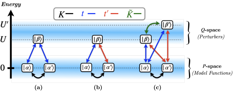
Figure 1: Schematic representation of the three different cases of interactions considered between the model and the perturber spaces. (a) Symmetric interaction between two degenerate model functions and a single perturber. (b) Asymmetric interactions between two degenerate model functions and a single perturber. (c) Asymmetric interactions between two degenerate model functions and two non-degenerate perturbers.

2 Two-step perturbative method: Rayleigh-Schrödinger and Brillouin-Wigner

The leading Brillouin-Wigner (BW) and Rayleigh-Schrödinger (RS) perturbation approaches [23] rely on the definition of an appropriate model space $P$ constructed on the model functions $\Bqty{\ket{\alpha}}$, eigenfunctions of the unperturbed Hamiltonian $\hat{H_{0}}$:

$$\hat{H}_{0}|\alpha\rangle=E_{\alpha}|\alpha\rangle$$ (1)

The orthogonal $Q$-space is spanned by the so-called $\{\ket{\beta}\}$ perturbers with energies $E_{\beta}=\matrixelement{\beta}{\hat{H}_{0}}{\beta}$. In a quasi-degenerate picture, the impact of the perturbation must be evaluated within the $P$-space first. In practice, the construction of an effective Hamiltonian $\hat{H}_{\mbox{\tiny eff}}$ that operates in the model space allows one to produce the associated effective model functions $\{\ket{\Psi^{\mbox{\tiny RS}}_{i}}\}$ (eigenvectors of $\hat{H}_{\mbox{\tiny eff}}$ in the $P$-space). At second order, the effective Hamiltonian matrix elements can be derived from the generalized Bloch equation:

$$\begin{split}\matrixelement{\alpha}{\hat{H}_{\mbox{\tiny eff}}^{(2)}}{\alpha^{\prime}}&=\delta_{\alpha\alpha^{\prime}}E_{\alpha^{\prime}}\\ &+\matrixelement{\alpha}{\hat{V}}{\alpha^{\prime}}\\ &+\sum_{\beta}^{\text{$Q$-space}}\frac{\matrixelement{\alpha}{\hat{V}}{\beta}\!\!\matrixelement{\beta}{\hat{V}}{\alpha^{\prime}}}{E_{\alpha^{\prime}}-E_{\beta}}\end{split}$$ (2)

It is well-known that the effective Hamiltonian is not hermitian. Such deviation arises from the summation in Eq. (2). Since the latter is expected to contribute less (i.e. second order) than the first and second terms, one can easily remedy this issue by averaging over the off-diagonal elements . Despite its approximate character, the diagonalization of the second order effective Hamiltonian $\hat{H}_{\mbox{\tiny eff}}^{(2)}$ generates qualitative effective model functions $\{\ket{\Psi^{\mbox{\tiny RS}}_{i}}\}$ and associated eigenvalues $\{E^{\mbox{\tiny RS}}_{i}\}$ resulting from the mixing of the $\{\ket{\alpha}\}$ through the perturbation $\hat{V}$. Importantly, this rotation within the $P$-space leaves the orthogonal states and the couplings within the $Q$ space unchanged. From this first step, a different PT partitioning of the Hamiltonian is introduced such that $\hat{H}=\hat{H}^{\mbox{\tiny RS}}+\hat{W}$, with

$$\hat{H}^{\mbox{\tiny RS}}=\sum_{i}^{\text{$P$-space}}E^{\mbox{\tiny RS}}_{i}\outerproduct{\Psi^{\mbox{\tiny RS}}_{i}}{\Psi^{\mbox{\tiny RS}}_{i}}+\sum_{\beta}^{\text{$Q$-space}}E_{\beta}\outerproduct{\beta}{\beta}$$ (3)

$\hat{W}$ is an improved perturbation operator in the sense that it should carry fewer significant contributions as compared to $\hat{V}$. Regarding the perturbation treatment, the expected improvement can be quantified by evaluating the ratio:

$$\begin{split}\tau=\frac{\rho_{\mbox{\tiny RSBW}}}{\rho_{\mbox{\tiny RS}}},\end{split}$$ (4)

where $\rho_{\mbox{\tiny RS}}$ and ${\rho_{\mbox{\tiny RSBW}}}$ quantify the perturbation contributions (respectively $\hat{V}$ and $\hat{W}$) over the reference unperturbed Hamiltonians (respectively $\hat{H}_{0}$ and $\hat{H}^{\mbox{\tiny RS}}$) at each step of the RSBW method, such that

$$\begin{split}\rho_{\mbox{\tiny RS}}=\frac{||\hat{V}||}{||\hat{H}_{0}||},\hskip 1.00006pt\mbox{ and }\hskip 1.00006pt\rho_{\mbox{\tiny RSBW}}=\frac{||\hat{W}||}{||\hat{H}_{\mbox{\tiny RS}}||},\end{split}$$ (5)

with the notation

$$\begin{split}||\hat{O}||=\left(\Tr\,[\hat{O}^{\dagger}\hat{O}]\right)^{1/2}\end{split}$$ (6)

for the norm of a generic operator $\hat{O}$ evaluated over the full $P+Q$ space [34]. The absence of degenerate states makes the BW theory particularly appealing with a straightforward expansion of the exact state energy $E_{i}$:

$$\begin{split}E_{i}=\matrixelement{\Psi_{i}}{\hat{H}}{\Psi_{i}}&+\sum_{n>1}\matrixelement{\Psi_{i}}{\hat{W}\hat{\Omega}^{\left(n-1\right)}}{\Psi_{i}}\end{split}$$ (7)

with

$$\hat{\Omega}^{\left(n\right)}=\left(\sum_{j\neq i}\frac{\outerproduct{\Psi_{j}}{\Psi_{j}}}{E_{i}-\hat{H}^{\mbox{\tiny RS}}}\hat{W}\right)^{\!\!n}.$$ (8)

In practice, the summation in Eq. (7) is truncated and the exact energy $E_{i}$ is approximated as $E^{\mbox{\tiny RSBW}}_{i}$ by setting the energy denominators to $E^{\mbox{\tiny RSBW}}_{i}-E^{\mbox{\tiny RS}}_{j}$ and $E^{\mbox{\tiny RSBW}}_{i}-E_{\beta}$:

$$\begin{split}E^{\mbox{\tiny RSBW}}_{i}&=\matrixelement{\Psi_{i}}{\hat{H}}{\Psi_{i}}\\ &+\sum_{j\neq i}^{\text{$P$-space}}\frac{\matrixelement{\Psi_{i}}{\hat{W}}{\Psi_{j}}\!\!\matrixelement{\Psi_{j}}{\hat{W}}{\Psi_{i}}}{E^{\mbox{\tiny RSBW}}_{i}-E^{\mbox{\tiny RS}}_{j}}\\ &+\sum_{\beta}^{\text{$Q$-space}}\frac{\matrixelement{\Psi_{i}}{\hat{W}}{\beta}\!\!\matrixelement{\beta}{\hat{W}}{\Psi_{i}}}{E^{\mbox{\tiny RSBW}}_{i}-E_{\beta}}\\ &+\ldots\end{split}$$ (9)

Importantly, the first summation in Eq. (9) accounts for the mixing of the model functions through the modified perturbation $\hat{W}=\hat{H}-\hat{H}^{\mbox{\tiny RS}}$. Not only does the RS treatment lift the quasi-degeneracy (see the energy denominators in Eq. (9), $E^{\mbox{\tiny RSBW}}_{i}-E^{\mbox{\tiny RS}}_{j}\approx E^{\mbox{\tiny RS}}_{i}-E^{\mbox{\tiny RS}}_{j}$) but it also involves $\hat{W}$ (instead of $\hat{V}$). The $E^{\mbox{\tiny RSBW}}_{i}$ values can be obtained from iterations on Eq. (9), including all terms at any arbitrary order. In the following, we will refer to the iter-RSBW method. When limited to first and second order contributions, the resulting quadratic equation can be further simplified by assuming $E^{\mbox{\tiny RSBW}}_{i}\approx E^{\mbox{\tiny RS}}_{i}$ in the energy denominators. This less demanding approach which should qualitatively validate the partitioning is named RSBW method.

By concentrating part of the perturbation in the redefinition of the zeroth-order Hamiltonian $\hat{H}_{\mbox{\tiny RS}}$ (given in Eq. (3)), one can expect (i) an improved convergence of the BW series as measured by $\tau<1$, (ii) a reduction of the number of iteration steps, and (iii) a reduced size-consistency error. In the following sections, the RSBW and iter-RSBW methods that combine RS and BW perturbation theories are exemplified on a model Hamiltonian built on a strictly degenerate two-dimensional $P$-space. The dimension of the orthogonal $Q$-space is varied to account for configuration interaction. Along our inspections, the quantities defined in Eq. (5) are evaluated to stress the method’s relevance and applicability.

3 Numerical results on model Hamiltonians

The energy splittings and the structure of the wavefunctions were examined on systems ruled by model Hamiltonians. To be demonstrative and to limit the number of parameters, we concentrated on a two-dimensional strictly degenerate model space spanned by the reference functions $\ket{\alpha}$ and $\ket{\alpha^{\prime}}$. The unperturbed Hamiltonian energies $\matrixelement{\alpha}{\hat{H}_{0}}{\alpha}=\matrixelement{\alpha^{\prime}}{\hat{H}_{0}}{\alpha^{\prime}}$ are set to zero whilst the perturbation within the $P$-space is $\matrixelement{\alpha}{\hat{V}}{\alpha^{\prime}}$. The model space interacts with the orthogonal space through $V_{\alpha\beta}=\matrixelement{\alpha}{\hat{V}}{\beta}$ and the perturbers $\left\{\ket{\beta}\right\}$ lie $E_{\beta}=\matrixelement{\beta}{\hat{H}_{0}}{\beta}>0$ higher in energy. Despite its simplicity, this picture is representative of the emblematic ”two electrons in two orbitals” problem (i.e. CAS[2,2]) encountered in bond dissociation processes and exchange coupling constants calculations. The $Q$-space affords for fluctuations with respect to a mean field description (e.g. inclusion of charge transfer configurations) and non-zero $V_{\beta\beta^{\prime}}=\matrixelement{\beta}{\hat{V}}{\beta^{\prime}}$ terms account for configuration interaction processes. Too small an $E_{\beta}$ value relatively to the energy splitting within the model space ($\propto|\matrixelement{\alpha}{\hat{H}}{\alpha^{\prime}}|$) makes $\ket{\beta}$ an intruder state that should be included in the model space. Evidently, the partitioning should then be reconsidered at the relatively small cost of an enlarged $P$-space. Without loss of generality, such a scenario will be avoided in the following by restricting the ranges of parameter variations.

For preliminary inspections, we considered a symmetric system characterized by a strictly degenerate model space coupled to a one-dimensional $Q$-space (see Figure 1(a)). This is the traditional one-band model used to interpret the physical mechanisms that govern the magnetic coupling. For this reason, the standard notations are introduced for the matrix elements with $t=V_{\alpha\beta}=V_{\alpha^{\prime}\beta}$, $K=\matrixelement{\alpha}{\hat{V}}{\alpha^{\prime}}$ and $U=\matrixelement{\beta}{\hat{H}_{0}}{\beta}>0$. From symmetry considerations, the exact model functions are the in-phase and out-of-phase linear combinations of the reference functions, $\ket{\Psi_{g}}=\frac{1}{\sqrt{2}}\left(\ket{\alpha}+\ket{\alpha^{\prime}}\right)$ and $\ket{\Psi_{u}}=\frac{1}{\sqrt{2}}\left(\ket{\alpha}-\ket{\alpha^{\prime}}\right)$. For the perturbative treatments to be valid, the absolute couplings $|t|$ between the $P$- and $Q$-spaces must be smaller than the energy separations between their respective states. Qualitatively, the splitting within the model space being ca. 2$|K|$, such conditions require $U\pm K>|t|$, setting the ranges of parameters we will use for numerical inspections. Following the Bloch theory [23], the second order effective Hamiltonian can be written as a dressed matrix :

$$\begin{split}\hat{H}_{\mbox{\tiny eff}}^{(2)}=\begin{pmatrix}-\frac{t^{2}}{U}&K-\frac{t^{2}}{U}\\ K-\frac{t^{2}}{U}&-\frac{t^{2}}{U}\\ \end{pmatrix}\end{split}$$ (10)

The eigenvalues $E^{\mbox{\tiny RS}}_{g}=K-2{t^{2}}/{U}$ and $E^{\mbox{\tiny RS}}_{u}=-K$ can be compared to the undressed model space energies $\pm K$. In general, $E^{\mbox{\tiny RS}}_{g}$ and $E^{\mbox{\tiny RS}}_{u}$ are a priori approximations of the exact energies of the full Hamiltonian $\hat{H}$. However, in the case under study, $E^{\mbox{\tiny RS}}_{u}$ is the exact energy for symmetry reasons ($\matrixelement{\Psi_{u}}{\hat{W}}{\beta}=0$). In contrast, the $\ket{g}$ state energy is modified through the second-order BW expansion (see Eq. (9)). Remembering that $\matrixelement{\Psi_{g}}{\hat{W}}{\Psi_{u}}=0$, no contribution arises from the mixing within the model space. Besides, the $Q$-space being one-dimensional and $\matrixelement{\beta}{\hat{W}}{\beta}=0$, the BW expansion ends at second-order with identically null higher-order terms :

$$\begin{split}E^{\mbox{\tiny RSBW}}_{g}=K\ +\ &\frac{2t^{2}}{E^{\mbox{\tiny RSBW}}_{g}-U}\end{split}$$ (11)

This quadratic equation is the one we would obtain from the exact diagonalization of the full Hamiltonian in the $\left\{\ket{\Psi_{g}},\ket{\beta}\right\}$ sub-space. This can be understood as follows: first, the symmetry of the problem fully defines the model functions $\ket{\Psi_{g}}$ and $\ket{\Psi_{u}}$, which makes any further expansion of the effective Hamiltonian unnecessary. Then, the BW treatment being exact at second order, Eq. (11) produces the exact energy. To avoid any iteration or quadratic equation resolution , $E^{\mbox{\tiny RSBW}}_{g}$ can be approximately evaluated by setting $E^{\mbox{\tiny RSBW}}_{g}$ to $E^{\mbox{\tiny RS}}_{g}=K-2{t^{2}}/{U}$ in the energy denominator (i.e. RSBW method).

RS	BW	RSBW
$28\%$	$6.7\%$	$3.9\%$

Table 1: Relative errors of the ground state energy of a symmetric system ($t=t^{\prime}$, Figure 1(a)) using the RS, BW and RSBW. $K=-1$, $t^{\prime}=-1$ and $U=2$ in $\lvert t\rvert$ unit.

Table 1 compares the relative errors for the ground state energy evaluated using the RS and RSBW approaches, and a BW-like correction to the $\ket{\Psi_{g}}$ state energy, $E^{\mbox{\tiny BW}}_{g}=K+{2t^{2}}/({K-U})$. Despite its simplicity, the model supports the two-step RSBW method which not only recovers the exact solution (see Eq. (11)), but also suggests a costless energy evaluation (3.9% relative error). The improved perturbation is measured by $\tau=0.6$ (see Eq. (5) with $K=-1$, $t^{\prime}=-1$ and $U=2$ in $\lvert t\rvert$ unit), highlighting the benefits brought by the $\hat{H}=\hat{H}^{\mbox{\tiny RS}}+\hat{W}$ splitting.

To complement these preliminary inspections, the method was then applied to a degenerate model-space interacting with a single perturber with $t=V_{\alpha\beta}\neq V_{\alpha^{\prime}\beta}=t^{\prime}$ (see Figure 1(b)). The dressed matrix given in Eq. (10) was modified accordingly, and subsequently diagonalized to produce the model functions $\ket{\psi_{1}}=\mbox{cos}(\theta)\ket{\alpha}+\mbox{sin}(\theta)\ket{\alpha^{\prime}}$ and $\ket{\psi_{2}}=-\mbox{sin}(\theta)\ket{\alpha}+\mbox{cos}(\theta)\ket{\alpha^{\prime}}$ and energies $E^{\mbox{\tiny RS}}_{1}$ and $E^{\mbox{\tiny RS}}_{2}$, with

$$\mbox{tan}(\theta)=\displaystyle\frac{U\sqrt{\Delta}+t^{2}-t^{\prime 2}}{UK-tt^{\prime}}$$ (12)

and

$$\Delta=\pqty{\frac{t^{2}+t^{\prime 2}}{2U}}^{2}+K\pqty{K-2\frac{tt^{\prime}}{U}}.$$ (13)

The absence of symmetry (i.e. $\theta\neq\frac{\pi}{4}$) gives rise to a non-zero $\matrixelement{\psi_{1}}{\hat{W}}{\psi_{2}}$ matrix element. Even though the BW expansion contains higher-order terms, it was truncated at second order for comparison purposes, and the exact energies $E_{i}$ were approximated as $E^{\mbox{\tiny RSBW}}_{i}$. Following the RSBW method (i.e. no iteration), the resulting quadratic equations were further simplified by setting the energy denominators to $E^{\mbox{\tiny RS}}_{i}-E^{\mbox{\tiny RS}}_{j}$ and $E^{\mbox{\tiny RS}}_{i}-U$ ($i,j=1,2$) in Eq. (9). From Figure 2, reasonably good agreement between the approximated $E^{\mbox{\tiny RSBW}}_{1}$ and $E^{\mbox{\tiny RSBW}}_{2}$ values and the exact ones is reached at the negligible cost of the redefinition of the zeroth-order Hamiltonian. Despite the similarity between the coupling value and the energy separation with the perturber ($t/\left(U+K\right)\sim-1$), the excited state energy is reproduced with a relative error smaller than 2% whatever the $K$ value.

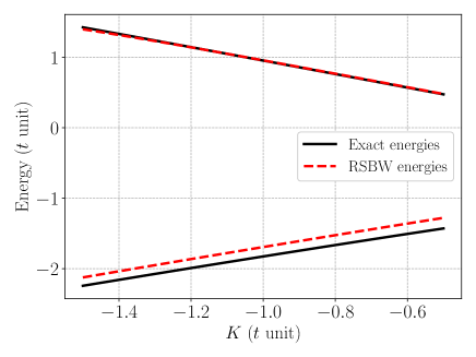
Figure 2: Ground and excited states energies $E^{\mbox{\tiny RSBW}}_{1}$ and $E^{\mbox{\tiny RSBW}}_{2}$ of an asymmetric system (Figure 1(b)) obtained from the second-order RSBW approach as a function of $K$ (all energies $E^{\mbox{\tiny RSBW}}_{i}$ in the energy denominators of Eq. (9) are set to $E^{\mbox{\tiny RS}}_{i}$). The exact energies are given for comparison. A single perturber lies $U=2$ higher above the degenerate model space, $t^{\prime}=-1.5$, and all energies are in $\lvert t\rvert$ unit.

However, a stronger deviation is observed for the ground state energy, a failure inherent to the BW approach that calls for a self-consistency procedure.

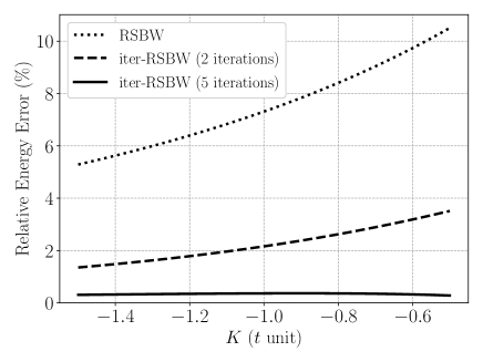
Figure 3: Relative error for the ground state energy of an asymmetric system (Figure 1(b)) obtained from the RSBW and iter-RSBW approaches as a function of $K$. A single perturber lies $U=2$ higher than the model space, $t^{\prime}=-1.5$, all energies are in $\lvert t\rvert$ unit.

Along the iter-RSBW method, the relative error becomes negligible (smaller than 0.4%) after a limited number of iterations (see Figure 3). The RSBW procedure is improved as supported by the $\tau$ values reported in Table 2.

$K$	-2	-1.5	-1
$\tau$	0.3	0.5	0.6

Table 2: $\tau$ values as defined in Eq. (4) stressing the improved convergence. $t^{\prime}=-1.5$ and $U=2$ in $\lvert t\rvert$ unit.

Let us stress that whatever the number of iterations, the strict BW approach limited to second-order fails to recover the transition energy $\Delta E=E_{2}-E_{1}$ with relative errors larger than 7%. Even though analytical solutions can be extracted, our intention is to stress the rapid convergence upon iterations, with a natural extension to higher orders in the BW expansion. For more realistic problems in quantum chemistry, the dimension of the $Q$-space would be larger. However, the size of the second order effective Hamiltonian (see Eq. (10)) remains unchanged and the decisive BW treatment is easily implemented with an improved convergence.

Finally, non-zero matrix elements $\tilde{K}=\matrixelement{\beta}{\hat{W}}{\beta^{\prime}}$ may couple perturbers within the $Q$-space in configuration interaction calculations (see Figure 1(c)). As a consequence, additional higher-order contributions are likely to emerge and can be easily evaluated due to the simplicity of the BW expansion. The same procedure was followed by first generating the model functions issued from the diagonalization of the second-order effective Hamiltonian. As expected, the second order iter-RSBW method fails to reproduce the exact energies (see Figure 4). Thus, the BW series was expanded up to third order contributions and iterations were carried out to evaluate the iter-RSBW states energies. Particular attention was paid to the third-order contributions involving $\tilde{K}$. The latter can be easily isolated in the BW expansion, excluding all the other third-order terms. After iterations, the truncated third order evaluation of the energies are referred to as truncated iter-RSBW. Interestingly, most of the missing dynamical correlation is faithfully recovered along this procedure. Such observation suggests that the iter-RSBW method allows one to concentrate the numerical effort on specific contributions. Let us finally mention that the transition energy $\Delta E$ evaluated from the truncated iter-RSBW is in excellent agreement (error smaller than 0.5%) with the exact value. The redefinition of the zeroth order Hamiltonian improves the BW convergence ($\tau=0.8$ for $K=-1$ in $\absolutevalue{t}$ unit) and sets a hierarchy in the third (and beyond) order contributions.

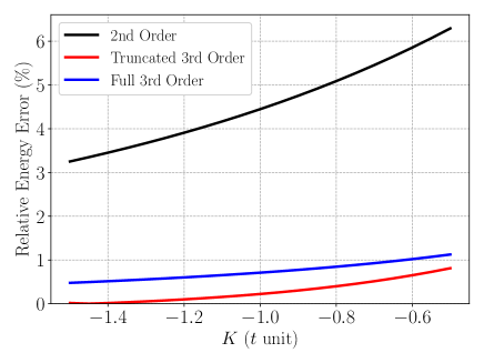
Figure 4: Relative error for the ground state energy of an asymmetric system (Figure 1(c)) obtained from the second order, truncated, and third order iter-RSBW approaches as a function of $K$. Two interacting perturbers, $\tilde{K}=-0.5$, lie $U=2$ and $U^{\prime}=3$ higher above the model space, $t^{\prime}=-1.5$. All energies are in $\lvert t\rvert$ unit.

4 Conclusion

The method we proposed combines the Rayleigh-Schrödinger (RS) and Brillouin-Wigner (BW) perturbation theories. The objective is to take advantage of both methods and to progressively include the perturbation effects. The relevance of this two-step strategy is evaluated on a series of model Hamiltonians. In the simplest symmetrical case, the analytical solution is retrieved. The construction of the second order effective Hamiltonian (model space) in the RS framework produces model functions. Even though this first step cannot safely account for the transition energy, a modified splitting of the Hamiltonian emerges with a redefinition of the perturbation. In the second step, a systematic and costless order-by-order BW treatment can be performed on each individual state (state-specific) and leads to accurate energy estimations. It is shown that the convergence of the BW energy expansion is improved, as featured by a reduction of the perturbation norm with respect to the zeroth order Hamiltonian. As soon as the perturbers interact in the orthogonal space (traditional CI structure), it is suggested that (i) a second order BW treatment fails to recover dynamical correlation effects, and (ii) the leading third order contributions involve couplings within the orthogonal space. An alternative approach would follow an iterated RS approach where the second step would consist in a redefinition of the model Hamiltonian. Depending on the size of the model space, the construction of successive effective Hamiltonians might become numerically demanding whereas the BW expansion is easily implemented at any order. Such extension and practical implementation for quantum chemistry Hamiltonians are left for future developments.

5 Acknowledgments

This work was supported by the Interdisciplinary Thematic Institute SysChem via the IdEx Unistra (ANR-10-IDEX-0002) within the program Investissement d’Avenir. The authors wish to thank Prof. C. Angeli for helpful discussions, and L. Petit for preliminary inspections and for furnishing the basis of the program used to generate the results presented in this article.

References

References

- [1] Helgaker T, Jorgensen P and Olsen J 2014 Molecular electronic-structure theory (John Wiley & Sons)
- [2] Levine D S, Hait D, Tubman N M, Lehtola S, Whaley K B and Head-Gordon M 2020 Journal of chemical theory and computation 16 2340–2354 URL https://doi.org/10.1021/acs.jctc.9b01255
- [3] Nakatani N and Guo S 2017 The Journal of Chemical Physics 146 URL https://doi.org/10.1063/1.4976644
- [4] Li Manni G, Smart S D and Alavi A 2016 Journal of chemical theory and computation 12 1245–1258 URL https://doi.org/10.1021/acs.jctc.5b01190
- [5] Roos B O, Taylor P R and Sigbahn P E 1980 Chemical Physics 48 157–173 URL https://doi.org/10.1016/0301-0104(80)80045-0
- [6] Siegbahn P, Heiberg A, Roos B and Levy B 1980 Physica Scripta 21 323 URL https://dx.doi.org/10.1088/0031-8949/21/3-4/014
- [7] Siegbahn P E, Almlöf J, Heiberg A and Roos B O 1981 The Journal of Chemical Physics 74 2384–2396 URL https://doi.org/10.1063/1.441359
- [8] Ding L, Knecht S and Schilling C 2023 arXiv preprint arXiv:2309.01676 URL https://doi.org/10.48550/arXiv.2309.01676
- [9] Yalouz S, Senjean B, Günther J, Buda F, O’Brien T E and Visscher L 2021 Quantum Science and Technology 6 024004 URL https://dx.doi.org/10.1088/2058-9565/abd334
- [10] Mizukami W, Mitarai K, Nakagawa Y O, Yamamoto T, Yan T and Ohnishi Y y 2020 Physical Review Research 2 033421 URL https://doi.org/10.1103/PhysRevResearch.2.033421
- [11] Mahler A D and Thompson L M 2021 The Journal of Chemical Physics 154 URL https://doi-org.scd-rproxy.u-strasbg.fr/10.1063/5.0053615
- [12] Ammar A, Scemama A and Giner E 2023 arXiv preprint arXiv:2303.02436 URL https://doi.org/10.48550/arXiv.2303.02436
- [13] Yalouz S and Robert V 2023 Journal of Chemical Theory and Computation 19 1388–1392 URL https://doi.org/10.1021/acs.jctc.2c01144
- [14] Yao Y and Umrigar C 2021 Journal of Chemical Theory and Computation 17 4183–4194 URL https://doi.org/10.1021/acs.jctc.1c00385
- [15] Barca G M, Gilbert A T and Gill P M 2018 Journal of chemical theory and computation 14 1501–1509 URL https://doi.org/10.1021/acs.jctc.7b00994
- [16] Wouters S and Van Neck D 2014 The European Physical Journal D 68 1–20 URL http://dx.doi.org/10.1140/epjd/e2014-50500-1
- [17] Keller S, Dolfi M, Troyer M and Reiher M 2015 The Journal of chemical physics 143 244118 URL https://doi.org/10.1063/1.4939000
- [18] Liu F, Kurashige Y, Yanai T and Morokuma K 2013 Journal of Chemical Theory and Computation 9 4462–4469 URL https://doi.org/10.1021/ct400707k
- [19] Chang C, Calzado C J, Amor N B, Marin J S and Maynau D 2012 The Journal of Chemical Physics 137 URL https://doi.org/10.1063/1.4747535
- [20] Amor N B and Maynau D 1998 Chemical physics letters 286 211–220 URL https://doi.org/10.1016/S0009-2614(98)00104-3
- [21] Roseiro P, Yalouz S, Brook D J, Ben Amor N and Robert V 2023 Inorganic Chemistry 62 5737–5743 URL https://doi-org.scd-rproxy.u-strasbg.fr/10.1021/acs.inorgchem.3c00275
- [22] Vela S, Verot M, Fromager E and Robert V 2017 The Journal of Chemical Physics 146 URL https://doi.org/10.1063/1.4975327
- [23] Lindgren I and Morrison J 2012 Atomic many-body theory vol 3 (Springer Science & Business Media)
- [24] Roos B O, Linse P, Siegbahn P E and Blomberg M R 1982 Chemical Physics 66 197–207 URL https://doi.org/10.1016/0301-0104(82)88019-1
- [25] Andersson K, Malmqvist P A, Roos B O, Sadlej A J and Wolinski K 1990 Journal of Physical Chemistry 94 5483–5488 URL https://doi.org/10.1021/j100377a012
- [26] Angeli C, Cimiraglia R, Evangelisti S, Leininger T and Malrieu J P 2001 The Journal of Chemical Physics 114 10252–10264 URL https://doi.org/10.1063/1.1361246
- [27] Angeli C, Cimiraglia R and Malrieu J P 2001 Chemical physics letters 350 297–305 URL https://doi.org/10.1016/S0009-2614(01)01303-3
- [28] Angeli C, Cimiraglia R and Malrieu J P 2002 The Journal of chemical physics 117 9138–9153 URL https://doi.org/10.1063/1.1515317
- [29] Li J, Jones B A and Kais S 2023 Science Advances 9 eadg4576 URL https://doi.org/10.1126/sciadv.adg4576
- [30] Yi J and Chen F 2019 The Journal of Chemical Physics 150 URL https://doi.org/10.1063/1.5081814
- [31] Hubač I, Wilson S, Hubač I and Wilson S 2010 Brillouin-Wigner methods for many-body systems (Springer)
- [32] Hubač I and Neogrády P 1994 Physical Review A 50 4558 URL https://doi.org/10.1103/PhysRevA.50.4558
- [33] Wilson S, Hubač I, Mach P, Pittner J and Čársky P 2003 Brillouin-wigner expansions in quantum chemistry: Bloch-like and lippmann-schwinger-like equations Advanced Topics in Theoretical Chemical Physics (Springer) pp 71–117
- [34] Golub G H and Van Loan C F 2013 Matrix computations (JHU press)