Causal Message-passing

Causal Message Passing: A Method for Experiments with Unknown and General Network Interference

Sadegh Shirani             Mohsen Bayati Graduate School of Business, Stanford University Randomized experiments are a powerful methodology for data-driven evaluation of decisions or interventions. Yet, their validity may be undermined by network interference. This occurs when the treatment of one unit impacts not only its outcome but also that of connected units, biasing traditional treatment effect estimations. Our study introduces a new framework to accommodate complex and unknown network interference, moving beyond specialized models in existing literature. Our framework, which we term causal message-passing, is grounded in a high-dimensional approximate message passing methodology and is specifically tailored to experimental design settings with prevalent network interference. Utilizing causal message-passing, we present a practical algorithm for estimating the total treatment effect and demonstrate its efficacy in four numerical scenarios, each with its unique interference structure.

Total treatment effect, network interference, approximate message-passing, experimental design

1 Introduction

Analysis of high-dimensional data within networks of interacting units has increasingly become a fundamental challenge for causal inference tasks, which aim to assess the efficacy of new policies or products. The gold standard approach commonly advocates for randomized experiments, which partition the target population into treatment and control groups. This method addresses the inherent limitations of observing solely the implemented treatment outcomes, while not having access to the counterfactual scenarios. Through randomized experiments, one can measure causal effects by comparing outcomes between treatment and control groups, yielding an unbiased estimate under the key assumption known as the Stable Unit Treatment Value Assumption (SUTVA) (Cox, 1958, Rubin, 1978).

According to the SUTVA, it is assumed that the outcome of a unit is independent of the treatment assignments of other units. While this assumption is reasonable in certain settings, it often breaks down in real-world scenarios where units interact (Sussman and Airoldi, 2017). Consider a study aiming to assess the effectiveness of a new medication for a contagious disease: the treatment group receives the medication while the control group is given a placebo. In such settings, accounting for the potential network effects among units (individuals in this context) is crucial. For instance, the disease may spread among units, thereby blurring the lines between them and complicating efforts to attribute observed outcomes exclusively to the medication. Therefore, it becomes essential to factor in the effects of network interference for accurately assessing treatment efficacy.

Violating the SUTVA necessitates the development of different techniques for measuring causal effects with minimal assumptions. However, by considering an arbitrary interference model, estimating any causal estimand becomes impossible as the model is not identifiable (Forastiere et al., 2022, Yu et al., 2022, Basse and Airoldi, 2018a , Karwa and Airoldi, 2018, Aronow and Samii, 2017, Manski, 2013). In particular, Karwa and Airoldi, (2018) demonstrate that under arbitrary interference, the number of potential outcomes for each individual may “explode.” Precisely, the cardinality of the set of distinct potential outcomes grows exponentially fast with the number of units in the experiment (Sussman and Airoldi, 2017). Additionally, Karwa and Airoldi, (2018) argue that estimation results are sensitive to model misspecifications caused by imposed assumptions. Hence, it is essential to relax the model assumptions while ensuring tractable estimation tasks to effectively study the causal inference problem under network interference.

The present study introduces a new framework for modeling and analyzing causal effects in the presence of network interference, drawing inspiration from statistical physics and message-passing algorithms (Gallager, 1962, Mezard et al., 1986, Mezard and Montanari, 2009). Specifically, within this context, information disseminates through a network of units via message exchanges. In high-dimensional networks with non-linear patterns of interference, we then employ the Approximate Message-Passing (AMP) methodology (Donoho et al., 2009, Bayati and Montanari, 2011) to prove that the dynamics of potential outcomes over time can be approximated by a one-dimensional state evolution equation. In light of this, we refer to our approach by Causal Message-Passing (Causal-MP).

The proposed framework has also a potential outcome interpretation (Imbens and Rubin, 2015). Specifically, at each time instant, the model represents the outcome for each unit as a weighted combination of non-linear functions applied to the outcomes of individuals in previous time periods, their treatment assignments, and their covariate vectors. This structure, reminiscent of neural networks, enables the model to adapt to broad families of network interference patterns.

The rigorous theoretical investigation of the proposed model, rooted in AMP literature, leads to the development of a new toolkit for the design and analysis of algorithms to study unobserved counterfactuals in the presence of network interference. The idea is to observe the outcomes and treatments of a system of connected individuals over time. By studying the system from the no-treatment state to a steady state, we gain valuable insights into sufficient information to estimate causal effects.

To demonstrate the practical relevance of the proposed approach, we study its application to multi-period Bernoulli randomized designs and present a simple practical algorithm for estimating the Total Treatment Effect (TTE). The TTE measures the difference in average outcomes between a scenario where the entire population is treated and one where all units are under control. We rigorously establish the strong consistency of our estimator in this setting and demonstrate its generalizability through extensive simulations. Notably, our estimation procedure operates without any observations of the individual units’ covariates. The considered setup aligns well with the current practices of many firms that adopt a dynamic framework for releasing new treatments, such as products or features, through a sequence of randomized experiments (Kohavi et al., 2020).

The rest of this article is organized as follows. We begin by illustrating the complexities and challenges of causal modeling of network interference through an example in § 1.1. In § 2, we review the existing literature and then proceed to present a detailed discussion of the proposed framework in § 3, including the main results and estimation algorithm for the TTE. The theoretical results and analysis of the presented framework are given in § 4, followed by extensive numerical studies in § 5. We conclude the article with further discussion on the modeling and analysis of the problem in §6-7. Finally, the appendices include detailed proofs and supplementary information to support the main content of the article.

1.1 Illustrative Example and Challenges in Modeling Network Interference

Figure 1: Illustration of temporal and spatial relationships in a causal inference problem.

Assume we seek to evaluate the effectiveness of a new medical treatment on the severity of a contagious disease by observing two units—or individuals in this context—across three time periods. Figure 1 uses circles to represent outcomes. The treatment induces multiple types of effects: a direct effect influencing the treated unit (unit 1); a treatment spillover effect that indirectly affects the control unit (unit 2); and a carryover effect that has lasting effects for future outcomes (Athey et al., 2018, Forastiere et al., 2022, Xiong et al., 2019). A comprehensive description of these effects is presented in Appendix 8. Beyond these, interactions between units give rise to unit peer effects and autocorrelation, each contributing additional layers of interference (Yu et al., 2022, Imai et al., 2019). Moreover, an anticipation effect is also present, wherein units’ current behavior is shaped by their expectations of future events.

A causal model should encapsulate these multifaceted effects while addressing a series of further challenges. First, identifying the structure of causal relationships in a network is intricate due to the complex interplay among units, especially when the interference structure remains either unknown or unobservable. Second, the patterns of interference are not static but evolve temporally, demanding models designed to capture such dynamics. Third, the efficacy of treatments varies over time, either waning or potentially amplifying, which calls for dynamic models that span multiple observational periods for precise evaluation. Fourth, practical limitations, such as budgetary constraints on the size of treatment groups, necessitate methodologies that can yield reliable inferences even from smaller data sets. Finally, the presence of noise and unobserved covariates adds a layer of complexity, warranting models that minimize the reliance on noisy or incomplete data.

Our proposed framework is a step towards addressing the complexities of multiple types of interference, including direct effect, treatment spillover effect, unit peer effect, autocorrelation, carryover effect, and anticipation effect, while also accommodating temporal variations in network structure and accounting for measurement errors. Its core thrust lies in distilling high-dimensional complexities into analyzable one-dimensional dynamics.

2 Other Related Literature

The assumption of no interference, known as SUTVA, is foundational in causal inference (Cox, 1958, Rubin, 1978, Manski, 1990, Sussman and Airoldi, 2017). However, recent research increasingly aims to relax this assumption. Some studies focus on testing for network interference (Aronow, 2012, Bowers et al., 2013, Saveski et al., 2017, Athey et al., 2018, Pouget-Abadie et al., 2019, Hu et al., 2022, Han et al., 2022), while others propose new assumptions and methods for estimating causal effects without SUTVA (Leung, 2020, Viviano, 2020, Leung, 2022, Yu et al., 2022, Cortez et al., 2022b , Cortez et al., 2022a , Agarwal et al., 2022, Belloni et al., 2022, Li and Wager, 2022a , Li and Wager, 2022b ). We will briefly survey these emerging developments and proceed by a brief discussion of the literature on approximate message-passing algorithms.

Neighborhood Interference Assumption.

The Neighborhood Interference Assumption (NIA) is a prominent approach in the literature for relaxing SUTVA, positing that an individual’s outcome is influenced solely by the treatments of neighboring units in the network (Sussman and Airoldi, 2017, Jiang and Wang, 2023). Studies have expanded upon NIA through various methodologies. With known or partially observed interference networks, works by Leung, (2020), Viviano, (2020), Agarwal et al., (2022), Belloni et al., (2022), Li and Wager, 2022b focus on nonparametric and regression estimators, experimental designs, and asymptotic behaviors. In the absence of known network structures, Cortez et al., 2022a , Cortez et al., 2022b , Yu et al., (2022) have proposed unbiased estimators under various experimental designs and constraints. Recently, Leung, (2022) introduced a more flexible concept of “Approximate Neighborhood Interference (ANI),” providing a weaker variant of NIA and demonstrating the consistency of inverse-probability weighting estimators under this new assumption. In this work, we do not make the NIA assumption.

Partial Interference.

The concept of partial interference serves as another notable avenue for relaxing SUTVA, where the population is partitioned into non-overlapping clusters without any network interference between them (Rosenbaum, 2007, Candogan et al., 2021). While extending this concept to complex networks, the bias in standard estimators is influenced by the number of inter-cluster edges (Yu et al., 2022). Strategies to mitigate this bias include cluster-randomized designs by Eckles et al., (2016) and graph cluster-randomized designs by Ugander et al., (2013), both of which necessitate knowledge of the interference network, a prerequisite not essential for the current study.

Restrictions on Interference Network.

In the literature, various constraints have been placed on interference structures beyond the NIA and partial interference. Studies such as Li and Wager, 2022a and Chin, (2018) focus on bounding the largest node degree and proving the asymptotic normality of certain estimators. Other works like Agarwal et al., (2022), Jagadeesan et al., (2020), and Wang et al., (2020) introduce methods based on unique observation patterns or localized interference. Known or restricted network topologies are considered by Viviano, (2020), Belloni et al., (2022), Cai et al., (2015), and Leung, (2022). Application-specific restrictions on interference patterns have been explored by Holtz et al., (2020), Wager and Xu, (2021), Munro et al., (2021), Johari et al., (2022), Farias et al., (2022), and Farias et al., (2023), encompassing contexts ranging from marketplaces to dynamical systems.

Single-time Point Observation.

The majority of existing literature on network interference has concentrated on single-time point observations, thereby observing each individual’s outcome once (Hudgens and Halloran, 2012, Aronow and Samii, 2017, Basse et al., 2019, Leung, 2020, Sävje et al., 2021, Li and Wager, 2022b , Yu et al., 2022, Cortez et al., 2022b , Leung, 2022). These works have advanced causal effect estimation and illuminated the intricacies of network interference in this setting. Recently, however, there is a pivot toward multi-time point observations (Li and Wager, 2022a , Boyarsky et al., 2023, Ni et al., 2023). In this evolving context, Li and Wager, 2022a discuss challenges and the utility of additional data, while Boyarsky et al., (2023) utilize temporal treatment variations to model interference. Ni et al., (2023) propose a randomized design in panel experiments that accommodates both spatial and temporal interference. The starting point of this work is also multi-period experiments and we then show how it can adapt to single-point observations.

Deterministic versus Stochastic Models.

Predominantly, the literature treats potential outcomes and network structures as deterministic, attributing randomness solely to treatment assignment (Aronow and Samii, 2017, Aronow, 2012, Athey et al., 2018, Basse et al., 2019, Leung, 2020, Sävje et al., 2021, Yu et al., 2022, Harshaw et al., 2022, Leung, 2022). However, recent studies have begun to incorporate stochastic elements. For instance, Li and Wager, 2022b employ random graph models, while Li and Wager, 2022a consider Bernoulli-distributed individual outcomes influenced by past outcomes and neighboring treatments. Cortez et al., 2022b introduce observation noise into the potential outcome model, and Li et al., (2021) analyze how network noise affects estimator bias and variance. In this work, we consider a stochastic model involving randomness for the outcomes, treatments, covariates, and the interference pattern.

Model-based Approaches and Limitations.

An alternative approach employs structured potential outcome models, commonly linear. For instance, studies by Goldsmith-Pinkham and Imbens, (2013), Blume et al., (2015), Yu et al., (2022), Belloni et al., (2022), Jiang and Wang, (2023) leverage linear models to account for interference. Similarly, Cai et al., (2015) models outcomes as linear in the proportion of treated neighbors, and other works focus on models linear in specific neighborhood statistics (Toulis and Kao, 2013, Basse and Airoldi, 2018b , Chin, 2019). However, this approach necessitates a priori knowledge of network topology to select and compute relevant statistics. A fundamental challenge is that such models may oversimplify complex social interactions, not capturing their full intricacies (Angrist, 2014). The model in this paper is aimed to capture more complex patterns of interference.

Approximate Message Passing (AMP).

The origins and underlying motivations for AMP can be traced back to Thouless et al., (1977), Kabashima, (2003), Donoho et al., (2009). The theoretical groundwork for AMP was laid by Bolthausen, (2014) and has since been expanded upon with various degrees of generality. An admittedly incomplete list includes Bayati and Montanari, (2011), Bayati et al., (2015), Javanmard and Montanari, (2013), Berthier et al., (2020), Chen and Lam, (2020), Zhong et al., (2021), Dudeja et al., (2023), Wang et al., (2022). For a more comprehensive overview, we refer the reader to Zdeborová and Krzakala, (2016), Montanari, (2018), Feng et al., (2022). Traditionally, AMP and state evolution have been employed to study high-dimensional estimation problems via the perspective of an iterative dynamical system. This system refers to a high-dimensional signal subjected to nonlinear transformations, which is then multiplied by an observed mixing matrix. The primary objective is to utilize the one-dimensional state evolution of the dynamics in order to refine the nonlinear functions, thereby enhancing the estimation accuracy of the evolving high-dimensional object. Our methodology, however, deviates from this norm. In our approach, both the mixing matrix and the nonlinear functions remain unobserved. Instead, we observe the actual outcomes, which represent the true signal. Subsequently, we utilize AMP and state evolution to deduce the sufficient statistics related to the mixing matrix and the nonlinear function. These statistics then guide us in estimating causal effects.

3 Problem Formulation and Main Results

In this section, we first present a potential outcome specification that captures an unknown general interference structure. Subsequently, we outline our main theoretical results, which provide the foundation for a practical algorithm to estimate causal effects. We also introduce an algorithm for estimating confidence intervals. Finally, we conclude this section by examining an application of Causal-MP in the context of the Bernoulli randomized design.

3.1 Potential Outcome Specification

Consider a setting with $N$ individuals indexed by $n\in[N]:=\left\{1,\ldots,N\right\}$ over a time horizon of $[T]_{0}:=\left\{0,1,\ldots,T\right\}$. At time instant $t>0$, each unit $n$ has been assigned a treatment decision denoted by $W^{n}_{t}$ which is distributed according to a probability distribution $\pi_{t}$. We refer to the set ${\cal E}=\{\pi_{1},\ldots,\pi_{T}\}$ as the experimental design and assume that for all $t$, the support of $\pi_{t}$ is a subset of the real line that includes $0$ and at least one non-zero element. Whenever $W^{n}_{t}=0$, we say that unit $n$ is under control; otherwise, we say unit $n$ receives the treatment. Then, we denote by $Y^{n}_{t}{({\cal E})}$ the outcome of unit $n$ at time $t$ under experimental design ${\cal E}$. We eliminate the notation ${\cal E}$ whenever there is no ambiguity. In addition, for a fixed integer $M$, we let the matrix $\bm{X}\in\operatorname{\mathbb{R}}^{M\times N}$ be the covariate matrix such that its $n^{th}$ column (denoted by ${\vec{X}}^{n}$) gives the characteristics of unit $n$ (e.g., age, gender, etc.).

To define the potential outcome specification, we let $\{g_{t}\}_{t\in[T]_{0}}$ be a family of unknown measurable functions such that $g_{t}:\operatorname{\mathbb{R}}\times\operatorname{\mathbb{R}}^{T}\times\operatorname{\mathbb{R}}^{M}\mapsto\operatorname{\mathbb{R}}$. For each $t$ and $n$, the output from $g_{t}$ is given as $g_{t}\left(Y^{n}_{t}{},\vec{W}^{n},{\vec{X}}^{n}\right)$. With a slight extension in notation, $g_{t}\big{(}\vec{Y}_{t}{},\bm{W}{},\bm{X}\big{)}$ represents a vector of size $N$, where the $n^{th}$ element is defined by $g_{t}\left(Y^{n}_{t}{},\vec{W}^{n},{\vec{X}}^{n}\right)$. Here, we denote $\vec{Y}_{t}{}=\big{(}Y^{1}_{t}{},\ldots,Y^{N}_{t}{}\big{)}^{\top}$ which is the column vector that contains the outcomes of all individuals at time $t$. We also let $\bm{W}{}\in\operatorname{\mathbb{R}}^{T\times N}$ such that the $n^{th}$ column denoted by $\vec{W}^{n}$ represents the treatment assignment of unit $n$ during the whole time horizon; that is, $\vec{W}^{n}=\big{(}W^{n}_{1},\ldots,W^{n}_{T}\big{)}^{\top}$. Then, given the vector of initial outcomes $\vec{Y}_{0}{}$, we define

$$\vec{Y}_{t+1}{}=\big{(}{\bf A}+{\bf B}_{t}\big{)}g_{t}\left(\vec{Y}_{t}{},\bm{W}{},\bm{X}\right)+\vec{\epsilon}^{\;}_{t},\quad\quad\quad t=0,1,\ldots,T-1,$$ (1)

where ${\bf A}$ and ${\bf B}_{t}$ are $N\times N$ matrices and $\vec{\epsilon}^{\;}_{t}=\big{(}\epsilon^{1}_{t},\ldots,\epsilon^{N}_{t}\big{)}^{\top}$. Here, the matrices ${\bf A}$ and ${\bf B}_{t}$ are unknown and capture the interference structure as follows. Let ${\text{A}}^{ij}$ and ${\text{B}}^{ij}_{t}$ denote the element in the $i^{th}$ row and $j^{th}$ columns of ${\bf A}$ and ${\bf B}_{t}$, respectively; the value ${\text{A}}^{ij}+{\text{B}}^{ij}_{t}$ quantifies the impact of unit $j$ on unit $i$ at time $t$. Following this intuition, henceforth, we refer to ${\bf A}$ and ${\bf B}_{t}$ as fixed interference matrix and time-dependent interference matrix, respectively. In addition, we let ${\bf G}_{t}={\bf A}+{\bf B}_{t}$ and refer to it as the interference matrix at time $t$. Then, the function $g_{t}$ represents the impact of past outcomes, treatment assignments, and covariates of individuals on their current outcomes. Finally, $\vec{\epsilon}^{\;}_{t}$ is the zero-mean noise term that accounts for misspecifications and measurement errors.

One can interpret the specification in Eq. (1) as follows: If we exclude the noise term $\vec{\epsilon}^{\;}_{t}$, the potential outcome for unit $n$ at time $t+1$ is a weighted combination of “messages” it receives from all other units. Each message is a (nonlinear) function of the outcome of the sending unit at time $t$, its entire treatment assignment, and its covariate vector. This is expressed as

$$Y^{n}_{t+1}{}=\sum_{i\in[N]}{\text{G}}^{ni}_{t}\underbrace{g_{t}(Y^{i}_{t}{},\vec{W}^{i},{\vec{X}}^{i})}_{\textbf{Message of $i$ to $n$}}\,.$$ (2)

The potential outcome $Y^{n}_{t+1}{}$ will subsequently be used in the message that unit $n$ sends to other units in future periods. Tracing back in time and interpreting each $Y^{i}_{t}{}$ as a weighted combination of the messages it receives from other units at time $t$, the impact of unit $i$ on unit $n$ is shaped by a combination of the impacts it receives from other units, combined with the treatment assignment and personal characteristics of unit $i$. This message exchange encapsulates the interference effect within the network of individuals.

It is worth noting that in the literature on message-passing algorithms, the message from unit $i$ to $n$ differs slightly from the description above. Specifically, the message from each unit $i$ to $n$ is as described, but it omits the message received from $n$ in the prior period. If we represent the message from unit $i$ to $n$ at time $t+1$ by $U^{i\rightarrow n}_{t+1}{}$, then $U^{i\rightarrow n}_{t+1}{}=g_{t}(\sum_{j\in[N]\setminus n}{\text{G}}^{ij}_{t}U^{j\rightarrow i}_{t}{},\vec{W}^{j},{\vec{X}}^{j})$. However, in the large $N$ regime, this is approximately equivalent to the simpler specification in Eq. (2). This approximation underpins the AMP algorithm. For completeness, we provide this heuristic argument, that has also appeared in AMP literature, in Appendix 9. Additionally, in the AMP literature, this exercise often leads to a dynamic as in Eq. (1) that also incorporates a memory term involving $g_{t-1}(\vec{Y}_{t-1}{},\bm{W}{},\bm{X})$, also known as the Onsager term. However, in our context, this term disappears since the matrix ${\bf G}_{t}$ is not symmetric.

In the context of the outcome specification presented in (1), an observation consists of panel data $\left\{Y^{n}_{t}{({\cal E})}\right\}_{n\in[N],t\in[T]_{0}}$ obtained from conducting an experiment involving $N$ units with experimental design ${\cal E}$. In this setting, individuals’ outcomes evolve over time, and the interference effect propagates through the network. Then, the specification (1) enables us to capture the interference effect by incorporating both the treatment spillover effect and the unit peer effect. This implies that the treatments and outcomes of all individuals can influence the outcome of any specific unit, thus relaxing the commonly employed neighborhood interference assumption in the network interference literature (Sussman and Airoldi, 2017). Moreover, Eq. (1) accounts for the cascading effect of interventions in the system, allowing individuals located far apart to influence each other’s outcomes through other units over multiple time periods. Therefore, this outcome model encompasses all types of effects depicted in Figure 1. In addition, the presence of each unit’s entire treatment assignment over time on the right-hand side of Eq. (1) encapsulates the anticipated effect discussed in $\S$ 1.1.

To facilitate the subsequent technical discussions, we let the entries of the interference matrices ${\bf A}$ and ${\bf B}_{t}$, as well as the elements of the noise vector $\vec{\epsilon}^{\;}_{t}$ be Gaussian random variables with unknown parameters. Entries of ${\bf A}$ are i.i.d. Gaussian random variables with mean $\mu/N$ and variance $\sigma^{2}/N$, independent from anything in the model. Similarly, for any $t\in[T]_{0}$, entries of ${\bf B}_{t}$ are i.i.d. Gaussian random variables with mean $\mu_{t}/N$ and variance $\sigma^{2}_{t}/N$, independent from all other sources of the randomness in the model. We note that, under Assumption 3.1, the variations in each matrix entry are of order $1/\sqrt{N}$, while its mean is of order $1/N$. This choice allows the variations to exert a dominant effect, thereby enabling the specification to capture heterogeneous patterns of interference. Elements of noise vector $\vec{\epsilon}^{\;}_{t}$ are i.i.d Gaussian random variables with mean zero and finite variance $\sigma_{e}^{2}$, independent from anything in the model.

In the subsequent sections, we will rigorously analyze the data generated by Eq. (1) under Assumptions 3.1 and 3.1. Our primary goal is to develop practical and effective algorithms to identify and estimate the underlying causal effects within this framework.

We will relax these assumptions in §5 by conducting extensive numerical analyses with different interference structures. This universality phenomenon aligns with findings in random matrix theory, AMP, and high-dimensional statistics literature and is discussed in §6. Moreover, §6 discusses settings where independence between the unit covariates $\bm{X}$ and the interference pattern is relaxed.

3.2 Causal Estimands

The literature has explored several estimands for causal effects, with a focus on average effects rather than individual-level effects (Han and Ugander, 2023, Yu et al., 2022, Li and Wager, 2022a , Leung, 2022, Sävje et al., 2021, Hu et al., 2022). Here, we aim to estimate the Total Treatment Effect (TTE), also known as Global Treatment Effect (GTE). This estimand specifically examines the average effect of altering the treatment for the entire community. For instance, in the case of a contagious disease, TTE quantifies the reduction in the number of infections or the impact on government health expenses when the new medication is administered to all individuals, as compared to a scenario where nobody receives it. Precisely, for any two designs of the experiment ${\cal E}_{1}$ and ${\cal E}_{2}$, we define

$$\text{TTE}_{t}{({\cal E}_{2},{\cal E}_{1})}=\lim_{N\rightarrow\infty}\frac{1}{N}\sum_{n=1}^{N}\big{(}Y^{n}_{t}{({\cal E}_{2})}-Y^{n}_{t}{({\cal E}_{1})}\big{)},$$ (3)

A notable special case arises when ${\cal E}_{1}$ and ${\cal E}_{2}$ represent experimental designs in which all treatment assignments are set to $0$ or $1$, respectively. With a slight abuse of notation, this is denoted by $\text{TTE}_{t}{(1,0)}$. In scenarios where only a single observation of the data is accessible, it is typically assumed that $t$ is sufficiently large for the effect to have stabilized. However, in this paper, we aim to estimate $\text{TTE}_{t}{(1,0)}$ for all values of $t$, which will allow us to trace the evolution of $\text{TTE}_{t}{(1,0)}$, even before stabilization.

The TTE is particularly relevant in scenarios where a decision maker aims to use the result of the experiment to determine whether everyone should receive the new treatment or not. Specifically, in cases where there are constraints on the treatment budget, decision-makers would seek to estimate the effect of treating the entire population (i.e., the TTE) based on data obtained from experiments involving a limited treatment group (Yu et al., 2022).

3.3 State Evolution of the Experiment

Consider a panel dataset denoted as $\left\{Y^{n}_{t}{({\cal E})}\right\}_{n\in[N],t\in[T]_{0}}$, which is generated according to the model specified in Eq. (1). The goal is to derive efficient estimators for the TTE defined in (3). By analyzing the TTE, we gain valuable insights into the magnitude and significance of the treatment’s influence on the whole population. To proceed, for all $t\geq 1$, we define

$$\nu_{t}{({\cal E})}:=\lim_{N\rightarrow\infty}\frac{1}{N}\sum_{n=1}^{N}Y^{n}_{t}{({\cal E})},\quad\quad\quad\quad\rho_{t}{({\cal E})}^{2}:=\lim_{N\rightarrow\infty}\frac{1}{N}\sum_{n=1}^{N}Y^{n}_{t}{({\cal E})}^{2}-\nu_{t}{({\cal E})}^{2}.$$ (4)

Specifically, $\nu_{t}{({\cal E})}$ represents the sample mean of the observed outcomes at time $t$ under experimental design ${\cal E}$, while $\rho_{t}{({\cal E})}$ denotes the corresponding standard deviation. Then, our main theoretical contribution lies in demonstrating how we can utilize this information to estimate the desired counterfactuals about the network of individuals. To this end, let $p_{\bm{X}}$ denote the empirical distribution of columns of the covariate matrix $\bm{X}$; therefore, $p_{\bm{X}}$ defines a probability distribution over $\operatorname{\mathbb{R}}^{M}$. Additionally, we denote by $\Pi$ the probability distribution of the treatments. This distribution $\Pi$ is a product distribution, denoted as $\Pi=\pi_{1}\times\ldots\times\pi_{T}$, where $\pi_{t}$ represents the probability distribution of the treatments at time $t$. Then, under some moment conditions concerning $p_{\bm{X}}$ and $\Pi$, for any continuous function with at most polynomial growth like $\psi$, we show that

$$\lim_{N\rightarrow\infty}\frac{1}{N}\sum_{n=1}^{N}\psi\big{(}Y^{n}_{t}{({\cal E})},\vec{W}^{n},{\vec{X}}^{n}\big{)}\;\stackrel{{\scriptstyle\mathclap{\mbox{\scriptsize a.s.}}}}{{=}}\;\mathbb{E}\left[\psi\big{(}\nu_{t}{({\cal E})}+\rho_{t}{({\cal E})}Z,\vec{W},{\vec{X}}\big{)}\right],$$ (5)

and

$$\nu_{t+1}{({\cal E})} \;\stackrel{{\scriptstyle\mathclap{\mbox{\scriptsize a.s.}}}}{{=}}\;(\mu+\mu_{t})\mathbb{E}\left[g_{t}\big{(}\nu_{t}{({\cal E})}+\rho_{t}{({\cal E})}Z,\vec{W},{\vec{X}}\big{)}\right],$$ (6)

$$\rho_{t+1}{({\cal E})}^{2} \;\stackrel{{\scriptstyle\mathclap{\mbox{\scriptsize a.s.}}}}{{=}}\;(\sigma^{2}+\sigma_{t}^{2})\mathbb{E}\left[g_{t}\big{(}\nu_{t}{({\cal E})}+\rho_{t}{({\cal E})}Z,\vec{W},{\vec{X}}\big{)}^{2}\right]+\sigma_{e}^{2},$$

where $Z\sim{\cal N}(0,1)$ is independent from $(\vec{W},{\vec{X}})\sim\Pi\times p_{\bm{X}}$. We note that equalities in (5) and (6) hold almost surely. Then, inspired by the literature on AMP algorithms, we refer to (6) as state evolution equations of the experiment. We provide the rigorous statements and related details in §4. Here, we discuss the intuition and implications derived from (5) and (6).

Note that we utilize the available data $\left\{Y^{n}_{t}{({\cal E})}\right\}_{n\in[N],t\in[T]_{0}}$ to compute the sample mean $\left\{\nu_{t}{({\cal E})}\right\}_{t\in[T]_{0}}$ and the sample standard deviation $\left\{\rho_{t}{({\cal E})}\right\}_{t\in[T]_{0}}$ using (4). These statistics serve as the basis for estimating complex functions involving individuals’ outcomes, treatment assignments, and covariates using Eq. (5). Having access to ${\cal E}$ and $p_{\bm{X}}$, the unknown parameters in the state evolution equations are denoted as ${\cal U}:=\left(\mu,\sigma,\{\mu_{t}\}_{t\in[T]_{0}},\{\sigma_{t}\}_{t\in[T]_{0}},\{g_{t}\}_{t\in[T]_{0}},\sigma_{e}\right)$. By estimating ${\cal U}$, we can estimate any desired average counterfactual, including the TTE defined in Eq. (3).

It is worth mentioning that our approach does not impose any constraints on the experimental design and does not require specific knowledge about interference structure. As a result, the state evolution equations, besides Eq. (5), offer a versatile framework for the causal analysis of panel data. Notably, Eq.(6) suggests that we can effectively compute various functions that are relevant to understanding the average behavior of individuals.

Overall, the framework presented in this section addresses the challenges of analyzing high-dimensional interconnected data by reducing it to the study of one-dimensional state evolution equations. However, the problem of estimating the unknown parameters ${\cal U}$ still needs to be tackled.

3.4 Causal Effects Estimation

In this section, we propose a meta algorithm for estimating causal effects, building on Eqs. (5) and (6). This is done by estimating the parameters ${\cal U}:=\left(\mu,\sigma,\{\mu_{t}\}_{t\in[T]_{0}},\{\sigma_{t}\}_{t\in[T]_{0}},\{g_{t}\}_{t\in[T]_{0}},\sigma_{e}\right)$ using the available data. We then utilize Eqs. (5) and (6) for a second time to compute the desired counterfactuals and estimands. In this regard, according to the available data and our specific research objectives, we can introduce constraints on the parameters of the outcome model (1) to facilitate the estimation procedure of ${\cal U}$. Algorithm 1 outlines a general scheme for estimating the causal effect in a scenario with experimental design ${\cal E}$. The algorithm is designed to estimate the total treatment effect when altering the design from ${\cal E}_{1}$ to ${\cal E}_{2}$.

Data: ${\cal E}_{1},{\cal E}_{2}$, $\left\{Y^{n}_{t}{({\cal E})}\right\}_{n\in[N],t\in[T]_{0}}$, ${\cal E}$, and $p_{\bm{X}}$.

Step 1: Data processing

Compute $\left\{\nu_{t}{({\cal E})},\rho_{t}{({\cal E})}\right\}_{t\in[T]_{0}}$ by Eq. (4).

Step 2: Parameters estimation

Estimate ${\cal U}:=\left(\mu,\sigma,\{\mu_{t}\}_{t\in[T]_{0}},\{\sigma_{t}\}_{t\in[T]_{0}},\{g_{t}\}_{t\in[T]_{0}},\sigma_{e}\right)$, guided by Eq. (6).

Step 3: TTE estimation

Compute $\left\{\nu_{t}{({\cal E}_{1})},\rho_{t}{({\cal E}_{1})}\right\}_{t\in[T]_{0}}$ and $\left\{\nu_{t}{({\cal E}_{2})},\rho_{t}{({\cal E}_{2})}\right\}_{t\in[T]_{0}}$ by Eq. (6).

for $t\leftarrow 1$ to $T$ do

      $\widehat{\text{TTE}}_{t}{({\cal E}_{2},{\cal E}_{1})}\leftarrow\nu_{t}{({\cal E}_{2})}-\nu_{t}{({\cal E}_{1})}$

      end for

     

     Result: $\left\{\widehat{\text{TTE}}_{t}{({\cal E}_{2},{\cal E}_{1})}\right\}_{t\in[T]_{0}}$

     

Algorithm 1 Causal Message-passing: TTE estimation under network interference

3.4.1 Explanation of Algorithm 1

Algorithm 1 presents a systematic and flexible framework for conducting the estimation process, which comprises three main steps explained below.

Step 1: Data processing.

The initial step of the algorithm focuses on data preprocessing, which involves transforming the data into a suitable format for further analysis. This step is essential for preparing the data and ensuring its compatibility with subsequent steps. The computational cost of this preprocessing step scales linearly with the number of units and results in the generation of two vectors of size $T+1$.

Step 2: Parameters estimation.

In the second step, we utilize the preprocessed data to estimate ${\cal U}$. To accomplish this, we can make use of a parametric function class for $\{g_{t}\}_{t\in[T]_{0}}$, and introduce simplifying assumptions about the interference matrices. By leveraging the observed outcomes and Eq. (6), we estimate the relevant parameters.

It is worth noting that we can consider more complex models by collecting richer data. For instance, if we can divide individuals into distinct clusters with minimal interference or conduct the experiment in multiple stages with different treatments, we can incorporate additional data into the estimation of ${\cal U}$. This allows for the use of more sophisticated outcome models that capture the intricacies of the data.

Step 3: TTE estimation.

In the final step, the algorithm estimates the total treatment effect by estimating the counterfactual scenarios with treatments assigned according to ${\cal E}_{1}$ and ${\cal E}_{2}$. The algorithm computes the difference between the average outcomes in these two scenarios, providing the TTE over the desired time horizon. It is important to note that the time horizon for estimating the TTE can differ from the time horizon of collecting the data.

Overall, Algorithm 1 is designed to estimate the total treatment effect by observing a specific scenario of the system and estimating the counterfactual scenarios. It should be noted that the designs ${\cal E}_{1}$ and ${\cal E}_{2}$ are arbitrary and at least one of the counterfactual scenarios cannot be directly observed. However, by leveraging the available data and estimation techniques, the algorithm provides an estimate of the TTE. It is worth mentioning that the same procedure can be adapted to estimate other estimands related to the system. In the next sections, we first discuss an algorithm for the estimation of the confidence interval of TTE and then we give a more concrete version of Algorithm 1 tailored to the context of Bernoulli randomized design.

3.5 Confidence Intervals

To guarantee the reliability of our TTE estimates, obtaining confidence intervals is important. While we defer a proper treatment of this topic to follow up studies, we describe a heuristic approach here that seems promising, based on the numerical studies in § 5. By utilizing the panel data $\left\{Y^{n}_{t}{({\cal E})}\right\}_{n\in[N],t\in[T]_{0}}$, we employ the state evolution equations (Eq. (6)) to devise a resampling-based heuristic for confidence interval estimation of the TTE. This method involves resampling unit outcomes and repeatedly using Algorithm 1 to approximate the TTE distribution, considering the outcome dependencies due to network interference.

Specifically, confidence interval computation involves a two-step method. For a given $q\in(0,1)$ and $B\in\mathbb{N}$, the first step is resampling the units $B$ times, with each unit’s inclusion based on an independent Bernoulli trial with probability $q$. Then, for each sample, Algorithm 1 is applied to estimate the TTE over the time horizon, yielding $B$ values of TTE estimates for each time $t$. The second step involves calculating the confidence interval using the mean and standard deviation of these estimated TTEs across the $B$ samples. Selecting $q$ balances the accuracy of each sample’s estimates, which increases with higher $q$, against the correlation between samples, which favors lower $q$ values. While a thorough analysis of this method is reserved for future work, our numerical results in $\S$ 5 suggest that selecting smaller $q$ as $N$ grows provide reasonable confidence intervals.

3.6 Application to Bernoulli Randomized Design

We consider a two-stage Bernoulli randomized experiment as a specific case of the experimental design. This approach aligns with the prevailing practice in many firms, where a dynamic phase release of the new treatment is carried out through a sequence of randomized experiments (Kohavi et al., 2020, Han et al., 2022). Subsequently, the time horizon is divided into two intervals: $\{0,1,\ldots,T_{1}\}$ and $\{T_{1}+1,\ldots,T_{1}+T_{2}\}$. In the first interval, a fraction of units equal to $\pi_{1}$ receives the treatment, while in the second interval, a fraction of units equal to $\pi_{2}\neq\pi_{1}$ receives the treatment. The main objective is to estimate the total treatment effect by comparing two scenarios: one where everyone is treated (which we represent by ${\cal E}_{2}=1$) and one where no one is treated (which we represent by ${\cal E}_{1}=0$) throughout the time horizon $[T]_{0}=\{0,1,\ldots,T=T_{1}+T_{2}\}$. It is important to note that both scenarios ${\cal E}_{1}=0$ and ${\cal E}_{2}=1$ are counterfactuals since we do not observe the outcomes under these specific treatment assignments. In this setting, with a little abuse of the notation, we denote the experimental design by ${\cal E}=\{\pi_{1},\pi_{2}\}$, and the collected data can be represented by $\left\{Y^{n}_{t}{({\cal E})}\right\}_{n\in[N],t\in[T]_{0}}$. Then, letting $\pi_{1}=0$ is equivalent to considering historical data with no experiment in the first stage.

Additionally, we consider approximation of the function $g_{t}$, described as follows:

$$g_{t}\left(Y^{n}_{t}{({\cal E})},\vec{W}^{n},{\vec{X}}^{n}\right) =\Delta^{n}+\Xi^{n}Y^{n}_{t}{({\cal E})}+\Lambda^{n}W^{n}_{t+1}+\Gamma^{n}Y^{n}_{t}{({\cal E})}W^{n}_{t+1}+(\vec{\Theta}^{n})^{\top}{\vec{X}}^{n},$$ (7)

where $\Delta^{n},\Xi^{n},\Lambda^{n},\Gamma^{n}\in\operatorname{\mathbb{R}}$ and $\vec{\Theta}^{n}\in\operatorname{\mathbb{R}}^{M}$ are unknown random objects independent of everything else. Eq. (7) is a first-order approximation of the function $g_{t}$ plus the second-order term $\Gamma^{n}Y^{n}_{t}{({\cal E})}W^{n}_{t+1}$. In this context, the random variable $\Delta^{n}$ represents the baseline effect of individual $n$, irrespective of any treatment or past outcome. The coefficients $\Xi^{n},\Lambda^{n},\Gamma^{n}$ correspond to the specific effects of the current outcome and treatment of unit $n$ on the future outcomes. Furthermore, the random vector $\vec{\Theta}^{n}$ captures the influence of the covariates of the unit $n$. It is important to note that all these coefficients are treated as random objects, specific to each unit. This differs from the existing literature, where the potential outcome and network structure are assumed to be deterministic (Aronow and Samii, 2017, Aronow, 2012, Athey et al., 2018, Basse et al., 2019).

Considering the contagious disease example from § 1.1, the expression $\Delta^{n}+\Xi^{n}Y^{n}_{t}{({\cal E})}+(\vec{\Theta}^{n})^{\top}{\vec{X}}^{n}$ represents the severity of symptoms in the absence of medication. It combines several components: $\Delta^{n}$ captures the inherent severity level of the disease, $\Xi^{n}Y^{n}_{t}{({\cal E})}$ reflects the influence of the current health condition on future health outcomes, and $(\vec{\Theta}^{n})^{\top}{\vec{X}}^{n}$ incorporates the impact of the individual specific covariates such as age, gender, etc., on their health condition. The term $\Lambda^{n}W^{n}_{t+1}+\Gamma^{n}Y^{n}_{t}{({\cal E})}W^{n}_{t+1}$ accounts for the effect of administering the new medication to individual $n$. The inclusion of the multiplicative term $\Gamma^{n}Y^{n}_{t}{({\cal E})}W^{n}_{t+1}$ allows the consideration that the efficacy of treatment can vary according to the severity of symptoms. This flexible modeling approach recognizes the potential heterogeneity in treatment effects, allowing for a more nuanced understanding of the impact of the new medication.

We also assume that the mean of the entries of the time-dependent interference matrix ${\bf B}_{t}$ is fixed and equal to $\mu_{0}$. This means that $\mu_{t}=\mu_{0}$ for $t=1,\ldots,T_{1}+T_{2}$. To simplify the notation, we denote the overall mean as $\mu=\mu+\mu_{0}$ and without loss of generality, by modifying the function $g_{t}$ up to a coefficient, we set $\mu=1$. This implies that while the interference pattern can vary over time, each individual maintains a consistent level of interactions throughout the entire time horizon. In the context of our example, it means that individuals may interact with different people on different days, but the overall amount of interaction remains constant over time.

3.6.1 Total treatment effect estimation over the entire time horizon

Algorithm 2 provides a step-by-step procedure for estimating the total treatment effect in the specified context. It utilizes data with two segments of lengths $T_{1}$ and $T_{2}$, where $\pi_{1}$ fraction of the units are randomly treated in the first segment and $\pi_{2}$ fraction of the units receive treatment in the second segment. Similarly to Algorithm 1, a preprocessing step is performed, followed by two linear regressions to estimate the required parameters in the second step. The algorithm then proceeds to estimate the counterfactual scenario of treating everyone and uses this information, along with the observed scenario, to estimate the TTE in the final step. Consistency of the resulting estimator is established in $\S$ 4, and further details and analyses are provided in the appendices.

Data: ${\cal E}_{1}=0,{\cal E}_{2}=1$, $\left\{Y^{n}_{t}{({\cal E})}\right\}_{n\in[N],t\in[T]_{0}}$, ${\cal E}=\{\pi_{1},\pi_{2}\}$, $p_{\bm{X}}$, $T_{1}$, and $T_{2}$.

Step 1: Data processing

for $t\leftarrow 0$ to $T$ do

      $\hat{\nu}_{t}{({\cal E})}\leftarrow\frac{1}{N}\sum_{n=1}^{N}Y^{n}_{t}{({\cal E})}$

      end for

     

     Step 2: Parameters estimation (by linear regression models)

     

     Regress $\big{(}\hat{\nu}_{1}{({\cal E})},\ldots,\hat{\nu}_{T_{1}}{({\cal E})}\big{)}$ on $\big{(}\hat{\nu}_{0}{({\cal E})},\ldots,\hat{\nu}_{T_{1}-1}{({\cal E})}\big{)}$ to get $b_{1}$ and intercept $a_{1}$

     Regress $\big{(}\hat{\nu}_{T_{1}+1}{({\cal E})},\ldots,\hat{\nu}_{T}{({\cal E})}\big{)}$ on $\big{(}\hat{\nu}_{T_{1}}{({\cal E})},\ldots,\hat{\nu}_{T-1}{({\cal E})}\big{)}$ to get $b_{2}$ and intercept $a_{2}$

     $(\widehat{\Xi},\widehat{\Gamma},\widehat{\Lambda})\leftarrow\left(\frac{1}{2}\left(b_{2}+b_{1}-\frac{(b_{2}-b_{1})(\pi_{2}+\pi_{1})}{\pi_{2}-\pi_{1}}\right),\frac{b_{2}-b_{1}}{\pi_{2}-\pi_{1}},\frac{a_{2}-a_{1}}{\pi_{2}-\pi_{1}}\right)$

     Step 3: TTE estimation by $(\widehat{\Xi},\widehat{\Lambda},\widehat{\Gamma})$

     

     $\hat{\nu}_{0}{(1)}\leftarrow\hat{\nu}_{0}{({\cal E})}$

     $\widehat{\text{TTE}}_{0}{(1,0)}\leftarrow 0$

     for $t\leftarrow 0$ to $T-1$ do

           if $t\leq T_{1}-1$ then

                $\hat{\nu}_{t+1}{(1)}\leftarrow\hat{\nu}_{t+1}{({\cal E})}+\widehat{\Xi}\left(\hat{\nu}_{t}{(1)}-\hat{\nu}_{t}{({\cal E})}\right)+\widehat{\Lambda}(1-\pi_{1})+\widehat{\Gamma}\left(\hat{\nu}_{t}{(1)}-\pi_{1}\hat{\nu}_{t}{({\cal E})}\right)$

                else

                     $\hat{\nu}_{t+1}{(1)}\leftarrow\hat{\nu}_{t+1}{({\cal E})}+\widehat{\Xi}\left(\hat{\nu}_{t}{(1)}-\hat{\nu}_{t}{({\cal E})}\right)+\widehat{\Lambda}(1-\pi_{2})+\widehat{\Gamma}\left(\hat{\nu}_{t}{(1)}-\pi_{2}\hat{\nu}_{t}{({\cal E})}\right)$

                     end if

                    

                    $\widehat{\text{TTE}}_{t+1}{(1,0)}\leftarrow\widehat{\Xi}\widehat{\text{TTE}}_{t}{(1,0)}+\widehat{\Lambda}+\widehat{\Gamma}\hat{\nu}_{t}{(1)}$

                     end for

                    

                    Result: $\left\{\widehat{\text{TTE}}_{t}{(1,0)}\right\}_{t\in[T]_{0}}$

Algorithm 2 TTE estimation under network interference: two-stage Bernoulli design

It is worth highlighting that the Algorithm 2 operates without the need for covariate estimation. Instead, it leverages the available observed data to directly extract the required information. This key attribute makes the algorithm particularly useful in scenarios involving unobserved covariates. By bypassing the inclusion of covariates in the estimation process, Algorithm 2 streamlines the analysis and mitigates potential biases and complexities associated with covariate observation or estimation.

While we impose certain restrictions on the structure of the functions $g_{t}$ in Eq. (7), it is important to note that these restrictions still encompass a wide range of linear and non-linear models that have been extensively studied in the existing literature (Sussman and Airoldi, 2017, Belloni et al., 2022, Li and Wager, 2022a , Yu et al., 2022). In addition, in $\S$ 5, we provide comprehensive numerical analysis to support the flexibility and adaptability of Algorithm 2. The data generating process in these examples does not obey the specifications assumed by Algorithm 2 and are designed to assess applicability of the the algorithm in estimating the TTE, even when the data is generated using more complex underlying structures.

Remark 3.1 (Incorporating Prior Information)

In applying Algorithm 2, performance can be improved by integrating prior information relevant to the data and setting at hand. For instance, during the update $\widehat{\text{TTE}}_{t+1}{(1,0)}\leftarrow\widehat{\Xi}\widehat{\text{TTE}}_{t}{(1,0)}+\widehat{\Lambda}+\widehat{\Gamma}\hat{\nu}_{t}{(1)}$, one might constrain the left hand side to specific sub-intervals of $\mathbb{R}$, informed by prior knowledge.

3.6.2 Total treatment effect estimation at the equilibrium:

Another application of the state evolution equations (6) is to establish an estimator for the TTE at equilibrium. This stands in contrast to Algorithm 2, which is tailored to estimate the total treatment effect over the entire time horizon. This equilibrium estimand, denoted as $\text{TTE}{(1,0)}$, characterizes the TTE as the time horizon extends towards infinity, formally expressed as $\lim_{T\rightarrow\infty}\text{TTE}_{T}{(1,0)}$. Subsequently, with access to two sets of observations of individuals’ outcomes at the equilibrium, denoted as $\vec{Y}{(\pi_{1})}$ and $\vec{Y}{(\pi_{2})}$, we define the following estimator:

$$\widehat{\text{TTE}}{(1,0)}=\frac{1}{\pi_{2}-\pi_{1}}\sum_{n=1}^{N}\frac{Y^{n}{(\pi_{2})}-Y^{n}{(\pi_{1})}}{N}.$$ (8)

The estimator presented in Eq. (8) is inspired by the work of Yu et al., (2022) and extends a version analyzed by them. They demonstrated that with access to average baseline outcomes before an experiment, a special case of this estimator is unbiased under the neighborhood interference assumption and a linear outcome model. Our adaptation, which utilizes the function family $g$ from Eq. (7), enables the examination of non-linear outcomes. We find that the estimator (8) is subject to bias, with the degree of bias linked to the expected values of $\mathbb{E}[\Gamma^{n}]$ and $\mathbb{E}[\Xi^{n}]$. The formal statement of this finding is laid out in § 4.3.

4 Technical Results and Proofs Overview

In this section, we first outline and discuss the technical assumptions required for our proofs. We then present the rigorous statements of our theoretical contributions. Notably, in § 4.1, we present a general result concerning the state evolution of high-dimensional network data, which follows the same structure as Eq. (1). Next, in § 4.2, we analyze Algorithm 2 and assess the consistency of the resulting estimator. We conclude in § 4.3 by studying TTE estimation at equilibrium.

4.1 Main Result: The State Evolution of High-dimensional Data

To proceed, we consider a sequence of systems indexed by $N$, representing the number of individuals in the system. We rewrite the outcome model in Eq. (1) as follows:

$$\vec{Y}_{t+1}{({\cal E};N)}=\Big{(}{\bf A}(N)+{\bf B}_{t}(N)\Big{)}g_{t}\left(\vec{Y}_{t}{({\cal E};N)},\bm{W}{(N)},\bm{X}(N)\right)+\vec{\epsilon}^{\;}_{t}(N).$$ (9)

In (9), the sequence of initial outcomes $\vec{Y}_{0}{({\cal E};N)}\in\operatorname{\mathbb{R}}^{N}$ and the experimental design ${\cal E}$ are given and we added the notation $N$ to different terms to emphasize the dimension of the quantities. Then, for any fixed $t>0$, we analyze the behavior of the elements in $\vec{Y}_{t}{({\cal E};N)}$ as the system size $N$ approaches infinity. This investigation provides us with valuable insights into the evolution of the outcomes and how they are influenced by the design of the experiment. Because ${\cal E}$ is fixed and known, we can simplify the notation in Eq. (9) by omitting the explicit mention of ${\cal E}$ and $N$ whenever there is no ambiguity.

To present the main results, we first establish several notations. For any vector $\vec{v}\in\operatorname{\mathbb{R}}^{n}$, we denote its Euclidean norm as ${\left\|\vec{v}\right\|}$. For a fixed $k\geq 1$, we define ${{\cal C}{\cal P}}(k)$ as the class of functions $f:\operatorname{\mathbb{R}}^{\ell}\rightarrow\operatorname{\mathbb{R}}$, for some $\ell\geq 1$, that are continuous and exhibit polynomial growth of order $k$. In other words, there exists a constant $c$ such that $|f({\vec{X}})|\leq c(1+{\|{\vec{X}}\|}^{k})$. Moreover, we consider a probability space $(\Omega,\mathbb{F},\mathbb{P})$, where $\Omega$ represents the sample space, $\mathbb{F}$ is the sigma-algebra of events, and $\mathbb{P}$ is the probability measure. We denote the expectation with respect to $\mathbb{P}$ as $\mathbb{E}$. Additionally, for any other probability measure $p$, we use $\mathbb{E}_{p}$ to denote the expectation with respect to $p$.

Next, we state an assumption that is standard in the AMP literature and then discuss them in the context of our experimental design problem. Fix $k\geq 2$. We assume that

1. For any $t\in[T]_{0}$, the function $g_{t}:\operatorname{\mathbb{R}}^{1+T+M}\rightarrow\operatorname{\mathbb{R}}$ is a ${{\cal C}{\cal P}}(\frac{k}{2})$ function.

2. Let $p_{N}$ be the empirical distribution of columns of $\bm{X}(N)$, then $p_{N}$ converges weakly to a probability measure $p_{\bm{X}}$ on $\operatorname{\mathbb{R}}^{M}$ such that $\mathbb{E}_{p_{\bm{X}}}\big{[}{\|{\vec{X}}\|}^{k}\big{]}<\infty$ and, as $N$ grows to $\infty$, $\mathbb{E}_{p_{N}}\big{[}{\|{\vec{X}}\|}^{k}\big{]}\rightarrow\mathbb{E}_{p_{\bm{X}}}\big{[}{\|{\vec{X}}\|}^{k}\big{]}$.

3. If $\vec{W}\sim\Pi$, then $\mathbb{E}\big{[}{\|\vec{W}\|}^{k}\big{]}<\infty$.

4. The sequence of initial outcomes $\vec{Y}_{0}{(N)}$, the treatment assignments $\bm{W}{(N)}$, the covariates $\bm{X}(N)$, and the function $g_{0}$ are such that for deterministic values $\nu_{1}{}$ and $\rho_{1}{}$, we have

   $$\nu_{1}{} =\lim_{N\rightarrow\infty}\frac{\mu+\mu_{0}}{N}\sum_{n=1}^{N}g_{0}\big{(}Y^{n}_{0}{},\vec{W}^{n},{\vec{X}}^{n}\big{)}<\infty\,,$$

   $$0<\rho_{1}^{2}{}-\sigma_{e}^{2} =\lim_{N\rightarrow\infty}\frac{\sigma^{2}+\sigma_{0}^{2}}{N}\sum_{n=1}^{N}g_{0}\big{(}Y^{n}_{0}{},\vec{W}^{n},{\vec{X}}^{n}\big{)}^{2}<\infty\,.$$

5. There exist a ${{\cal C}{\cal P}}(\frac{k}{2})$ function $\bar{g}_{0}:\operatorname{\mathbb{R}}^{T+M}\mapsto\operatorname{\mathbb{R}}$ such that for all $t$ and for any ${{\cal C}{\cal P}}(\frac{k}{2})$ function $\varphi:\operatorname{\mathbb{R}}^{T+M}\mapsto\operatorname{\mathbb{R}}$, we have

   $$\lim_{N\rightarrow\infty}\frac{1}{N}\sum_{n=1}^{N}g_{0}\big{(}Y^{n}_{0}{},\vec{W}^{n},{\vec{X}}^{n}\big{)}\varphi(\vec{W}^{n},{\vec{X}}^{n}) \;\stackrel{{\scriptstyle\mathclap{\mbox{\scriptsize a.s.}}}}{{=}}\;\mathbb{E}\left[\bar{g}_{0}\big{(}\vec{W},{\vec{X}}\big{)}\varphi(\vec{W},{\vec{X}})\right]\,,$$

   $$\mathbb{E}\left[\bar{g}_{0}(\vec{W},{\vec{X}})^{2}\right] \leq\frac{\rho_{1}^{2}-\sigma_{e}^{2}}{\sigma^{2}+\sigma_{0}^{2}}\,,$$

   where $(\vec{W},{\vec{X}})\sim\Pi\times p_{\bm{X}}$.

Assumption 4.1 encompasses a set of regularity conditions on the system parameters and model attributes. Specifically, Part (i) ensures that the functions $g_{t}$ do not exhibit fast explosive behavior, guaranteeing the well-posedness of the large system asymptotics. Part (ii) is a standard assumption, ensuring that the empirical distribution $p_{N}$ remains stable and does not diverge as the sample size increases. This assumption holds, for instance, when unit covariates (e.g., the columns of the covariate matrix $\bm{X}$) are i.i.d. with distribution $p_{\bm{X}}$ with finite moments of order $k$. Moreover, Assumption 4.1-(iii) holds for a wide range of treatment assignments, including cases where the support of $\Pi$ is bounded, such as the Bernoulli design.

Assumption 4.1-(iv) is required for the proofs and rules out too restrictive initial conditions. For example, it is satisfied if the sequence of initial outcomes $\vec{Y}_{0}{}$ is drawn from a distribution that possesses finite moments of order $k$. Moreover, Assumption 4.1-(iv) means that the function $g_{0}$ is non-degenerate and ensures that the initial observations are informative and contribute to the estimation process.

Regularity conditions related to the outcome functions are commonly found in the existing literature. For example, in Sävje et al., (2021), the authors assume bounded moments of a certain degree for the potential outcome functions. In Leung, (2022), the assumption is made that outcomes are bounded, and Li and Wager, 2022b assume boundedness of the potential outcome function and its derivatives.

We proceed by considering the state evolution equations in (6); given $\nu_{1}{}$ and $\rho_{1}{}$ as in Assumption 4.1, for $t\geq 1$, we rewrite the state evolution equations as follows:

$$\nu_{t+1}{}:=(\mu+\mu_{t})\mathbb{E}\left[g_{t}\big{(}\nu_{t}{}+\rho_{t}{}Z,\vec{W},\vec{X}\big{)}\right],\quad\quad\rho_{t+1}^{2}{}:=(\sigma^{2}+\sigma_{t}^{2})\mathbb{E}\left[g_{t}\big{(}\nu_{t}{}+\rho_{t}{}Z,\vec{W},\vec{X}\big{)}^{2}\right]+\sigma_{e}^{2},$$ (10)

where $Z\sim{\cal N}(0,1)$ is independent from $(\vec{W},\vec{X})\sim\Pi\times p_{\bm{X}}$. Then, we present the following theorem that rigorously formalizes a more general version of the result we previously stated in $\S$ 3.3. This theorem also characterizes the joint distribution of $Y^{n}_{1}{},\ldots,Y^{n}_{t+1}{}$ within large sample asymptotics, providing a deeper understanding of the underlying statistical properties of a high-dimensional network data.

Theorem 4.1

Fixing $k\geq 2$, assume the sequence of initial outcomes $\vec{Y}_{0}{(N)}$, the treatment assignment $\bm{W}{(N)}$, as well as the covariates $\bm{X}(N)$ are given and suppose Assumption 4.1 holds. Then, we have the following statements for all $t\geq 0$.

1. For any function $\psi:\operatorname{\mathbb{R}}^{t+1+T+M}\mapsto\operatorname{\mathbb{R}}$ that $\psi\in{{\cal C}{\cal P}}(k)$, we have

   $$\;\lim_{N\rightarrow\infty}\frac{1}{N}\sum_{n=1}^{N}\psi\big{(}Y^{n}_{1}{},\ldots,Y^{n}_{t+1}{},\vec{W}^{n},{\vec{X}}^{n}\big{)}\;\stackrel{{\scriptstyle\mathclap{\mbox{\scriptsize a.s.}}}}{{=}}\;\mathbb{E}\Big{[}\psi\big{(}\nu_{1}{}+\rho_{1}{}Z_{1},\ldots,\nu_{t+1}{}+\rho_{t+1}{}Z_{t+1},\vec{W},{\vec{X}}\big{)}\Big{]},$$ (11)

   where $Z_{s}\sim{\cal N}(0,1),\;s=1,\ldots,t+1,$ are independent of $(\vec{W},{\vec{X}})\sim\Pi\times p_{\bm{X}}$.

2. The following equations hold and all limits exist, are bounded, and are deterministic (constant) random variables.

   $$\lim_{N\rightarrow\infty}\frac{1}{N}\sum_{n=1}^{N}Y^{n}_{t+1}{}\;\stackrel{{\scriptstyle\mathclap{\mbox{\scriptsize a.s.}}}}{{=}}\;\nu_{t+1}{},\quad\quad\quad\lim_{N\rightarrow\infty}\frac{1}{N}\sum_{n=1}^{N}Y^{n}_{t+1}{}^{2}\;\stackrel{{\scriptstyle\mathclap{\mbox{\scriptsize a.s.}}}}{{=}}\;\nu_{t+1}^{2}{}+\rho_{t+1}^{2}{}.$$ (12)

3. Let $\bm{V}_{t}$ be a matrix with columns equal to $Y_{s}{},\;s=1,\ldots,t$; that is $\bm{V}_{t}:=\left[Y_{1}{}\big{|}Y_{2}{}\big{|}\ldots\big{|}Y_{t}{}\right]$. Then, the following matrix is positive definite almost surely:

   $$\lim_{N\rightarrow\infty}\frac{\bm{V}_{t}^{\top}\bm{V}_{t}}{N}-\lim_{N\rightarrow\infty}\frac{\bm{V}_{t}^{\top}\bm{1}_{N\times 1}}{N}\lim_{N\rightarrow\infty}\frac{\bm{1}_{1\times N}\bm{V}_{t}}{N}\succ 0,$$ (13)

   where $\bm{1}_{l_{1}\times l_{2}}$ is matrix of size $l_{1}\times l_{2}$ with all entries equal to $1$.

We present a more detailed version of Theorem 4.1 in the appendices, accompanied by a complete proof. In the following discussion, we provide intuition, implications, and an overview of the proof.

Broadly speaking, Theorem 4.1 yields concise one-dimensional dynamical equations that consolidate the analysis of high-dimensional network data in the large sample asymptotic. Specifically, Eq. (LABEL:eq:BT-average_limit) indicates that individuals’ outcomes follow a Gaussian distribution at any given time. Moreover, when considering the entire time horizon, the outcomes exhibit a non-degenerate multivariate normal distribution (Eq. 13). This implies that the joint distribution of outcomes can be well-characterized and analyzed. In summary, Theorem 4.1 provides a framework for analyzing high-dimensional network data. It establishes the Gaussian nature of outcomes, facilitating the computation of various statistics and functions that capture the average behavior of the system.

To obtain the results of Theorem 4.1, the main challenge arises from the dependence between the fixed interference matrix ${\bf A}$ and individuals’ outcomes $\left\{Y^{n}_{t}{}\right\}_{n\in[N]}$ for any time $t>0$. Indeed, the observed outcomes reveal some information about ${\bf A}$ that we need to incorporate into any calculation concerning future observations. To overcome this obstacle, we leverage the “conditioning technique” introduced by Bolthausen, (2014) and developed further by Bayati and Montanari, (2011). This technique is commonly employed in the literature on Approximate Message Passing (AMP) algorithms, e.g., (Javanmard and Montanari, 2013, Rush and Venkataramanan, 2018, Berthier et al., 2020, Feng et al., 2022). They typically consider a fixed symmetric coefficient matrix or a Wishart matrix, with entries of order $O(1/\sqrt{N})$, and also assume a pseudo-Lipschitz non-linearity.

We adapt the conditioning technique to the current setting, considering a non-centered coefficient matrix with both fixed and time-dependent components. We also assume that the coefficient matrix is non-symmetric, dropping the Lipschitz assumption of non-linearity, and consider an additional noise term (denoted by $\vec{\epsilon}^{\;}_{t}$) in each round. As a result, the analysis becomes easier in some sense (as there is no “Onsager term”), yet different and involving additional randomness structures. The analysis technique, similar to the above literature, makes use of two versions of the Law of Large Numbers (LLN) and utilizes the invariance property of the Gaussian distribution under rotations.

4.2 Consistency of the TTE Estimator in Algorithm 2

We proceed by demonstrating that Algorithm 2 yields a strongly consistent estimator for the total treatment effect defined in (3).

Theorem 4.2

Let $\widehat{\text{TTE}}_{t}{(1,0)}$ be the estimator defined in Algorithm 2. Then, $\widehat{\text{TTE}}_{t}{(1,0)}$ is a strongly consistent estimator for the total treatment effect; that is, for any $t\in[T]_{0}$, we have

$$\lim_{N\rightarrow\infty}\widehat{\text{TTE}}_{t}{(1,0)}\;\stackrel{{\scriptstyle\mathclap{\mbox{\scriptsize a.s.}}}}{{=}}\;\text{TTE}_{t}{(1,0)}.$$ (14)

According to Theorem 4.2, as the number of individuals $N$ grows large, the estimator converges to the true value of the TTE almost surely.

We can establish a similar consistency result for the estimator in Algorithm 1 as long as the estimation of parameters in the second step remains consistent. A proof scheme analogous to Theorem 4.2, relying on the results of Theorem 4.1 and the state evolution dynamics in (10), would be sufficient to obtain these results. In summary, by appropriately choosing the model specifications and accurately estimating the set ${\cal U}$ in the second step of Algorithm 1, we can leverage the proposed framework to design and analyze various desired causal effects in diverse models. This claim is supported in $\S$ 5 through a comprehensive analysis of different systems with more general interference patterns that relax the assumptions of Theorem 4.2.

4.3 Analysis of the TTE Estimator at Equilibrium

Considering the Bernoulli design outlined in $\S$ 3.6, we can use the state evolution equations and Theorem 4.1 to analyze the performance of the estimator described in Eq. (8) as $T$ approaches infinity, representing the equilibrium state. However, note that we cannot let $T\rightarrow\infty$ as the results of Theorem 4.1 hold true for finite values of $T$. Therefore, we formally assume that for some sufficiently large value of $T$, the quantity $\text{TTE}_{T}{(1,0)}$ stabilizes, and we denote its value as $\text{TTE}{(1,0)}$. For any experimental design ${\cal E}$, we also denote $\hat{\nu}{({\cal E})}:=\frac{1}{N}\sum_{n=1}^{N}Y^{n}_{T}{({\cal E})}$; that is the sample mean at the equilibrium state under design ${\cal E}$. We then have the following result.

Theorem 4.3

Let $\widehat{\text{TTE}}{(1,0)}$ be the estimator defined by Eq. (8). Then, for any two values of $\pi_{2}\neq\pi_{1}$, we have:

$$\lim_{N\rightarrow\infty}\widehat{\text{TTE}}{(1,0)}\;\stackrel{{\scriptstyle\mathclap{\mbox{\scriptsize a.s.}}}}{{=}}\;\text{TTE}{(1,0)}+\frac{\gamma}{1-\xi}\lim_{N\rightarrow\infty}\left(\frac{\pi_{2}\hat{\nu}{(\pi_{2})}-\pi_{1}\hat{\nu}{(\pi_{1})}}{\pi_{2}-\pi_{1}}-\hat{\nu}{(1)}\right),$$ (15)

where $\xi=\mathbb{E}[\Xi^{n}]$ and $\gamma=\mathbb{E}[\Gamma^{n}]$.

The following corollary can be readily obtained as a special case of Theorem 4.3.

Corollary 4.4

If $\gamma=0$, then, $\widehat{\text{TTE}}{(1,0)}$ is a strongly consistent estimator for the total treatment effect at the equilibrium $\text{TTE}{(1,0)}$.

Given access to historical data before the experiment, and by setting $\pi_{1}=0$ in Theorem 4.3, we can simplify the bias term to $\frac{\gamma}{1-\xi}\left(\hat{\nu}{(\pi_{2})}-\hat{\nu}{(1)}\right)$. Consequently, if we can establish bounds on the values of $\gamma$, $\xi$, and $\hat{\nu}{(1)}$ based on system characteristics, we can place bounds on the bias of the estimation using the estimator in Eq. (8).

5 Numerical Illustrations

In this section, we investigate four experimental scenarios utilizing a Bernoulli design and employ Algorithm 2 to estimate the total treatment effect. We also use the resampling idea outlined in § 3.5 to estimate confidence intervals. The first scenario involves a linear-in-means model under a staggered roll-out design. The second scenario considers a binary potential outcome model, and the third scenario focuses on estimating the total effect of speeding up servers in a queueing system.

In each scenario, we consider populations of sizes $N=500$, $N=2,000$, and $N=10,000$. We conduct a two-stage experiment with varying lengths: once with $T_{1}=T_{2}=30$ observation periods, and once with $T_{1}=T_{2}=50$. The design employed in each case is detailed subsequently. To begin each experiment from a realistic, all-control state, we run the data generating process for $10$ “burn-in” periods before the start of the experimentation phase. This entire process is replicated $5,000$ times, with each replication involving a new realization of the randomized treatment assignment and the noise. Consequently, in every scenario, we compare the estimated TTE to its ground-truth value, accessible because we have control over the data-generating process and can recreate the necessary counterfactual outcomes.

5.1 Linear-in-Means Model with Staggered Roll-out Design

We begin by adapting and replicating the linear-in-means model (Leung, 2022, Hu et al., 2022, Cai et al., 2015). However, we make slight modifications to the original static model to capture dynamic settings. Specifically, we define the following dynamic potential outcome model:

$$Y^{i}_{t+1}{}=\alpha+\beta\frac{\sum_{j=1}^{N}E_{ij}Y^{j}_{t}{}}{\sum_{j=1}^{N}E_{ij}}+\delta\frac{\sum_{j=1}^{N}E_{ij}W^{j}_{t}}{\sum_{j=1}^{N}E_{ij}}+\gamma W^{i}_{t}+\varepsilon_{i},\quad\quad i\in[N].$$ (16)

In Eq. (16), the matrix $\bf E$ defines the adjacency matrix of an undirected graph. Following the method proposed by Leung, (2022), we generate the graph with adjacency matrix $\bf E$ using random geometric graph models. Specifically, we create a graph with vertex set $[N]$, such that for each pair of distinct units $i$ and $j$ in $[N]$, we define $E_{ij}=\mathds{1}_{\|\vec{V}_{i}-\vec{V}_{j}\|\leq r_{N}}$, where for each unit $n$ in $[N]$, $\vec{V}_{n}=[V_{n}^{1},V_{n}^{2}]^{\top}\in\operatorname{\mathbb{R}}^{2}$ is determined by independently sampling each coordinate from the uniform distribution over the interval $[0,1]$, and $r_{N}=\sqrt{\kappa(\pi N)^{-1}}$. Additionally, $\varepsilon_{n}=V_{n}^{1}-0.5+{\cal N}(0,1)$, with $(\alpha,\beta,\delta,\gamma,\kappa)=(-1,0.8,1,1,8)$ as parameters. Here, $\alpha$ signifies the baseline effect, $\beta$ indicates the autocorrelation and unit peer effect, $\delta$ reflects the treatment spillover effect, and $\gamma$ corresponds to the direct effect, as shown in Figure 1. Importantly, this model implies an average connectivity where each individual is linked to 8 other units, observing that $E_{nn}=0$ for all $n\in[N]$, which implies a moderate level of interference. Moreover, as Leung, (2022) notes, the noise term in (16) generates unobserved homophily, as units with closer $V_{n}^{1}$ values have similar outcomes.

To deliver the treatments, we have employed a staggered roll-out design, which involves incrementally spreading the treatments over two stages. The probabilities of receiving treatment in the two stages are set as $(\pi_{1},\pi_{2})=(0.2,0.5)$. Under this design, each unit that receives treatment in the first stage remains under treatment in the second stage as well. This assumption takes into account practical constraints that might prevent units from switching between control and treatment groups. In certain scenarios, once units undergo treatment, they may be unable to revert to the control group due to the presence of permanent effects or the irreversibility of the treatment, as discussed by Xiong et al., (2019). For example, in the context of a contagious disease, the new treatment can induce long-lasting effects on the treated individuals, making it impractical or ethically challenging to reverse the treatment once it has been applied.

Figure 2 displays the results from 5,000 data replications. The first row depicts experiments with $T=60$, while the second illustrates longer experiments with $T=100$. This figure presents both the average estimated TTE, obtained using Algorithm 2 along with its (true) 95% confidence interval, and the average ground-truth TTE derived from the replications. Additionally, Figure 2 includes the (estimated) 95% confidence intervals for the output of Algorithm 2, calculated via the heuristic detailed in § 3.5 using $B=500$. The parameter $q$ is set to $0.4$, $0.3$, and $0.25$ corresponding to $N=500$, $2,000$, and $10,000$, respectively. Finally, in light of Remark 3.1, we incorporate a “prior-knowledge” that the magnitude of the TTE is $100$.

As $N$ or $T$ grow in Figure 2, we observe more accurate estimation. The former directly aligns with the consistency result in Theorem 4.2. The latter is also (but indirectly) related to Theorem 4.2. Particularly, the inputs to Algorithm 2 contain error terms, that go to zero with $N$. For any finite $N$, their impact on the estimation error is compensated with increasing $T$. This indicates that as we gather more data over an extended period, the accuracy of the estimates further improves, as reflected in the lower width of the confidence intervals in the figure.

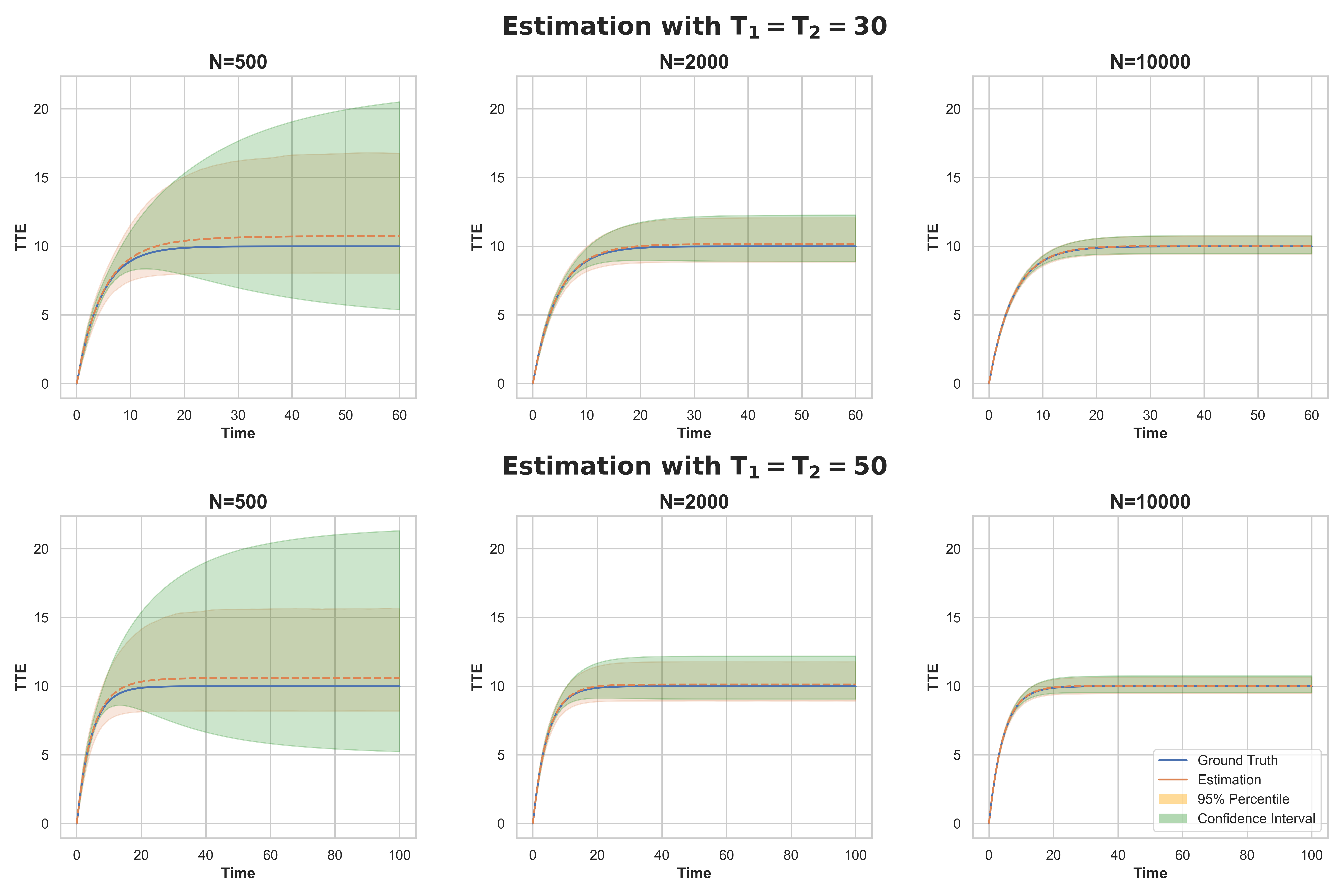
Figure 2: Linear-in-means model with staggered roll-out: 95% confidence intervals for the total treatment effect estimation when $(\pi_{1},\pi_{2})=(0.2,0.5)$.

5.2 Binary Outcome Model with Micro-Randomized Trial

The setting we examine next is a binary potential outcome model proposed by Li and Wager, 2022a under a Micro-Randomized Trial (MRT), where interventions are assigned to individuals in a sequential manner at multiple decision points throughout the experiment. Precisely, consider the following setup:

$$Y^{i}_{t+1}{}\sim\text{Bernoulli}\Big{(}\alpha+\beta W^{i}_{t}Z_{i}(t)+\gamma Y^{i}_{t}{}Z_{i}(t)+\delta W^{i}_{t}Y^{i}_{t}{}Z_{i}(t)\Big{)},$$ (17)

where $Z_{i}(t)=\sum_{j=1}^{N}E_{ij}Y^{j}_{t}{}$ represents the number of neighbors of individual $i$ with an outcome of 1. Following Example 1 in Li and Wager, 2022a , we let $\bf E$ to be the adjacency matrix of an Erdös-Rényi graph where each pairs of vertices are connected, independently, with probability $p_{\text{edge}}$. Considering Assumptions 3-5 in Li and Wager, 2022a and to ensure the uniqueness of the stationary distribution of the underlying system, we set the parameter values as $(\alpha,\beta,\gamma,\delta,p_{\text{edge}})=(0.5,0.04,0.04,0.01,3/N)$. Consequently, on average, each individual is connected to three other units, resulting in a low interference level in the network.

We adopt a micro-randomized trial with a Bernoulli design to determine the treatment group in each period. Specifically, we set $(\pi_{1},\pi_{2})=(0.25,0.75)$, and for each period in stage $j\in\{1,2\}$, we generate a new treatment vector $\vec{W}_{t}$ such that $W^{i}_{t}\;\stackrel{{\scriptstyle\mathclap{\mbox{\scriptsize iid}}}}{{\sim}}\;\text{Bernoulli}(\pi_{j})$, where $t\in[T_{j}]$. MRTs were initially introduced as an experimental design for developing just-in-time adaptive interventions by Liao et al., (2016) and Klasnja et al., (2015). Since then, they have gained popularity in various research areas, particularly in studying mobile health interventions aimed at increasing physical activity among sedentary individuals Klasnja et al., (2019).

Figure 3 presents the results of estimating the total treatment effect across 5,000 data replications, considering the outcome model defined by Eq. (17). Similar to Figure 2, we increase $N$ within each row and the $T$ within each column. Algorithm 2 successfully estimates the TTE with minimal bias. Notably, increasing both the sample size and the time horizon leads to significantly improved precision in the estimates. Here, $B=500$ and $q=0.7$ for all $N$ as due to low interference there is less need for lowering $q$ with $N$. Given the binary outcome model, we incorporate the prior knowledge that the TTE’s magnitude is capped at 1, as discussed in Remark 3.1.

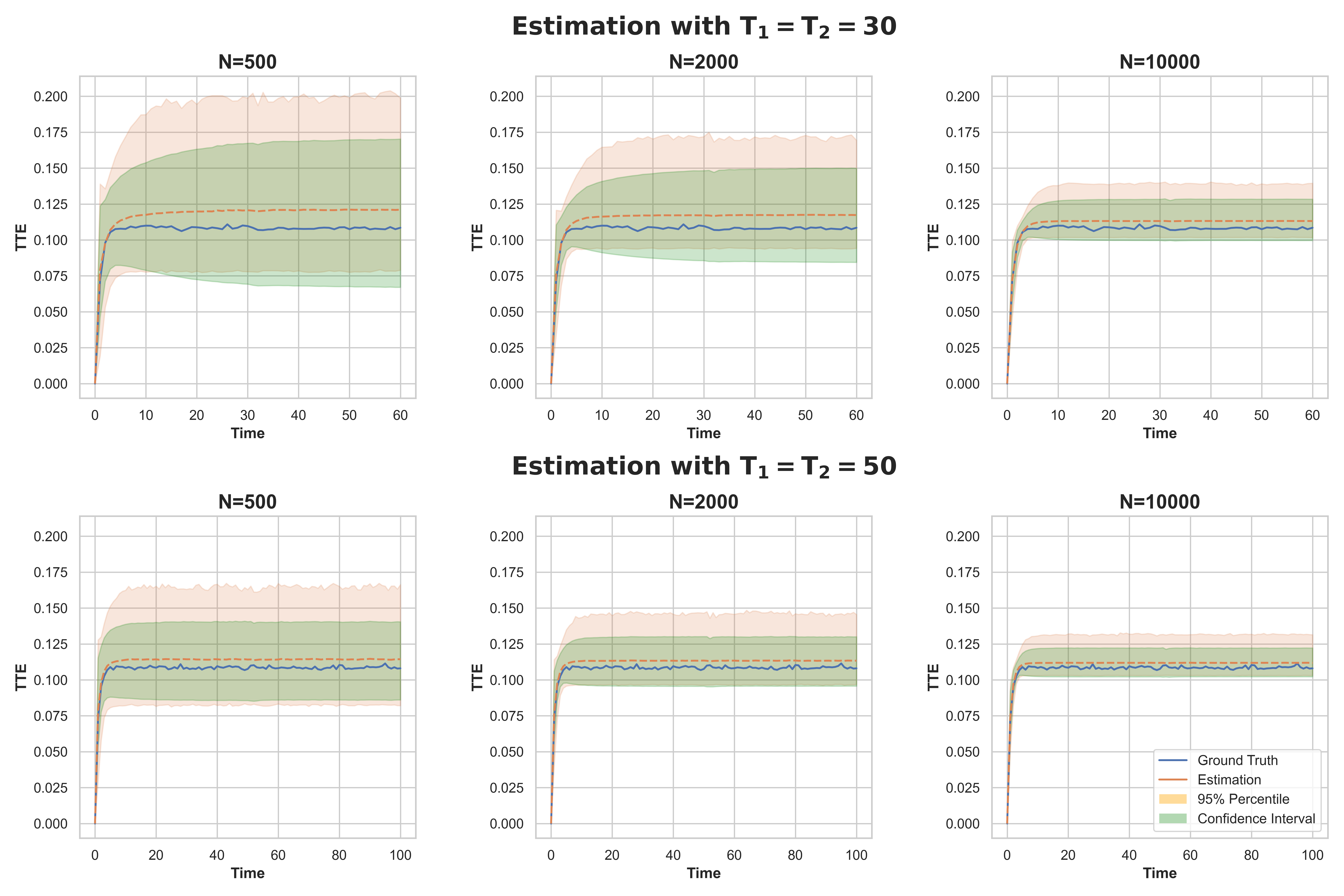
Figure 3: Binary outcome model with micro-randomized trial: 95% confidence interval for the total treatment effect estimation when $(\pi_{1},\pi_{2})=(0.25,0.75)$.

5.3 Server Speed-up Effect

We next consider a queueing system with $N$ servers that operates under the join-the-shortest queue policy, a widely adopted routing strategy for server farms Gupta et al., (2007). This policy assigns each incoming job to the shortest queue, and in cases where multiple queues are equally short, a random selection mechanism is employed. Motivated by Kuang and Mendelson, (2023), our primary focus is on understanding the interference impact of change in the service rate (speeding up the servers in our case) on the overall “server utilization”. To study this, we conduct a randomized experiment by speeding up selected servers. However, it is crucial to account for the interference effect among servers, which arises due to the join-the-shortest queue policy. This interference can cause servers in the control group, maintaining their original service rates, to experience reduced demand as a result of the allocation policy. Consequently, the treatment assignment impacts the control group.

We generate the data by simulating an ${\sf M/M/N}$ queueing system with an arrival rate of $0.95N$ and a service rate of 1 on each server. The treatment we consider involves doubling the speed of randomly selected servers. At the beginning of stage 1 ($t=1$), we increase the service rate of each server to 2 with a probability $\pi_{1}=0.15$, continuing this setting until the end of the first stage ($t=T_{1}$). Subsequently, at the beginning of stage 2 ($t=T_{1}+1$), we increase the service rate of each server to 2 with a probability $\pi_{2}=0.5$. While a server may be treated in the first stage and serve as a control in the second stage, its treatment status remains unchanged within each stage. Then, the observed data from server $n$ at time period $t$ (i.e., the outcome $Y^{n}_{t}{}$) represents the total time that server $n$ is busy during the time interval $[t,t+1)$. This setup allows us to evaluate the performance of Algorithm 2 in a setting with implicit interference introduced by the join-the-shortest queue policy, versus the more explicit specifications as in Eqs. 16-17.

Figure 4 presents the results of estimating the TTE in 5,000 replications of the system with different numbers of servers and time horizons. Despite the implicit and indirect interference caused by the allocation policy, Algorithm 2 successfully estimates the small treatment effect, even when treating at most half of the units in the system ($\pi_{2}=0.5$). This demonstrates the effectiveness of our proposed framework for real-world applications, as it accounts for the complex interference effects and yields reliable estimates of treatment effects in diverse scenarios. For the confidence interval heuristic, we set $B=500$ as before and $q$ is selected to be $0.2$, $0.15$, $0.1$ for $N=500$, $N=2000$, and $N=10000$, respectively. Consistent with earlier scenarios, we utilize the prior knowledge that the TTE must be between $-1$ and $0$, as noted in Remark 3.1.

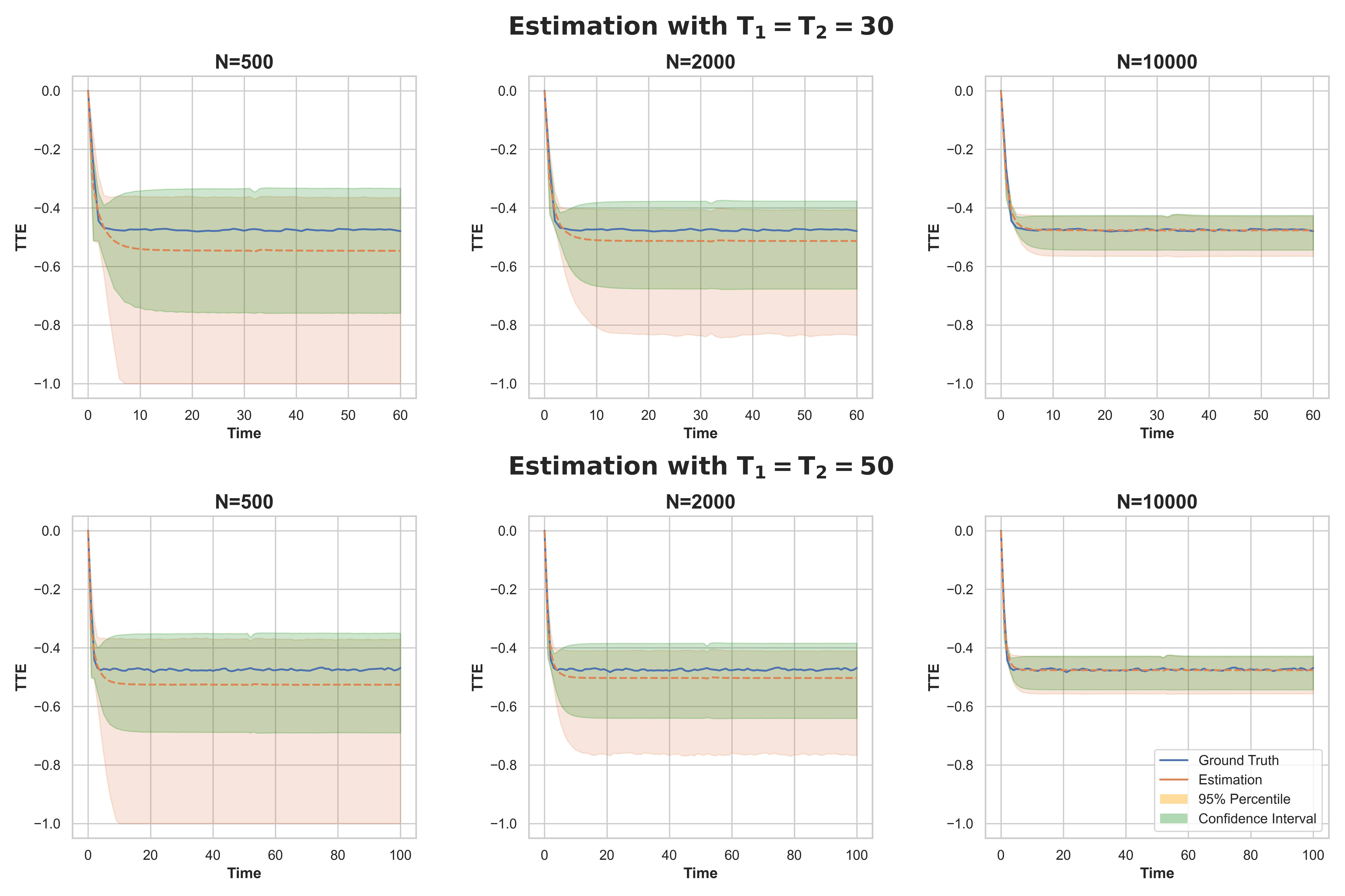
Figure 4: Server speed-up problem under a Bernoulli design: 95% confidence interval for the total treatment effect estimation when $(\pi_{1},\pi_{2})=(0.15,0.5)$.

5.4 Linear-in-Means Model with Facebook Friends Lists Network

In the final scenario, we explore the linear-in-mean model as described in (16), but utilize a Facebook (Meta) network dataset with 4,039 nodes and 88,234 edges, obtained from Leskovec and Mcauley, (2012). To adapt this network to our framework, we assume observation noise $\epsilon_{n}=\mathcal{N}(0,1)$ and implement a staggered roll-out design as in § 5.1. Then, Figure 5 displays the results. The right plot in this figure illustrates the degree distribution of the nodes, highlighting significant variation in the network. The confidence interval parameters $B$ and $q$ are $500$ and $0.15$, respectively. It is worth noting that the slight bias observed is potentially due to the relatively small network size ($N=$ 4,039) or misspecifications between the assumptions of our proposed methodology and the real network data. But the overall performance demonstrates the versatility of the proposed approach.

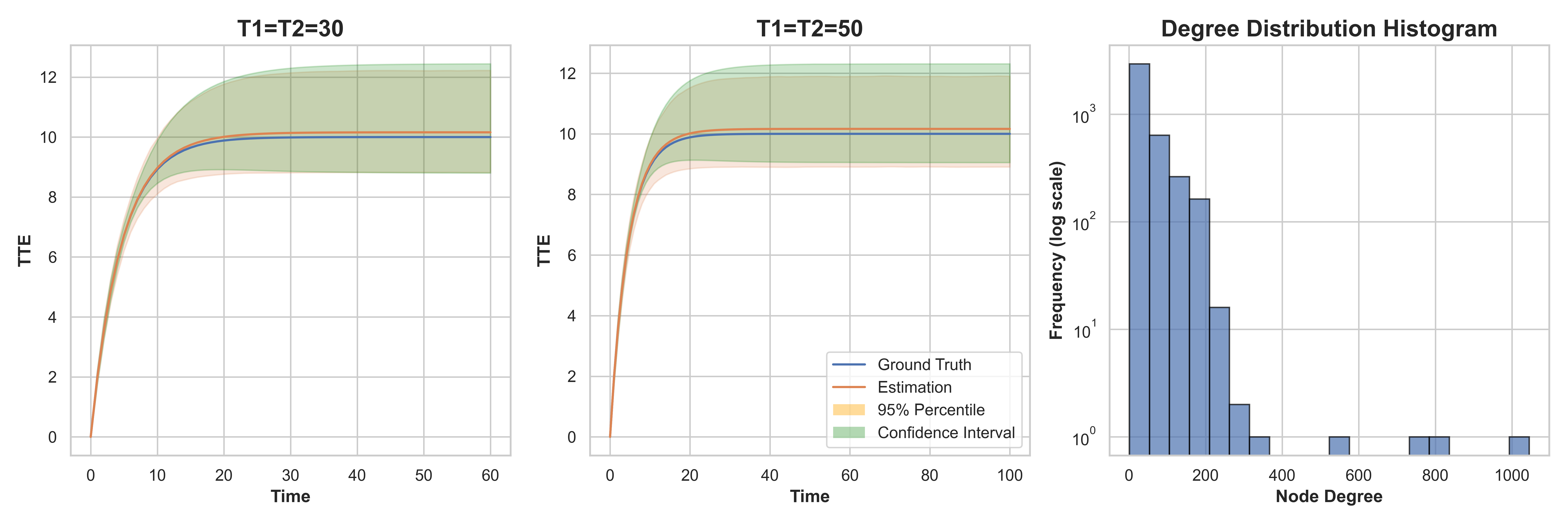
Figure 5: Left: Linear-in-means model with staggered roll-out, 95% confidence interval for the total treatment effect estimation when $(\pi_{1},\pi_{2})=(0.2,0.5)$. Right: degree distribution of the Facebook network.

6 Further Interpretations and Extensions

In this section, we first look at a neural network interpretation of the outcome specification 1 and then briefly discuss extensions to more general interference patterns.

6.1 Neural network interpretation

An alternative approach to interpret the specification (1) is motivated by the neural networks (Goodfellow et al., 2016) and may explain the empirical performance of Causal-MP in § 5, particularly its flexibility in capturing a wide range of outcome and interference patterns. Precisely, for a fixed $t>0$, the potential outcome of the $n^{th}$ unit at time $t$, $Y^{n}_{t}{}$, is equal to the result of applying non-linear transformations to the outcomes of all units during previous time steps, weighted by linear operators. Figure 6 illustrates this, in a simpler setting without covariates and static interference patterns. Mathematically, Eq. (1) captures this interpretation and $Y^{n}_{t}{}$ is the output of a neural network with $t+1$ layers (consisting of 1 input layer, $t-1$ hidden layers, and 1 output layer), where the input data is $\vec{Y}_{0}{}$. In this context, the elements of the interference matrix correspond to the weights in the neural network.

The neural network depiction of Eq. (1), alongside the proven ability of neural networks to encapsulate complex and nonlinear interactions—especially as discussed in the context of randomly weighted neural networks (Rahimi and Recht, 2007)—offers a promising avenue to study the Causal-MP framework. However, a distinct aspect of our approach, as informed by Eq. (5), is that as the number of units grows, our emphasis shifts to the estimation of the neural network’s sufficient statistics regarding its weights, rather than the estimation of each individual weight.

Figure 6: Illustration of the potential outcome specification (1) as a neural network model.

6.2 Structured interference

Consider the outcome specification 1. In certain situations, it is possible that the assumption of the independence between the interference matrices ${\bf A}$ and ${\bf B}_{t}$ and the covariates $\bm{X}$ may not hold. For example, if there exists spatial interference among units and the covariates contain information related to individuals’ home location, it would violate the last statement of Assumption 3.1. In such cases, a possible approach is to consider structured interference patterns that capture such spatial correlations.

6.3 Distribution of the interference matrix

The field of approximate message passing (AMP) encompasses studies on interference matrices with entries as independent random variables, each possessing finite moments and distinct distributions Bayati et al., (2015), Montanari and Venkataramanan, (2021), Berthier et al., (2020), Chen and Lam, (2020). This includes scenarios where the interference matrix belongs to the family of rotationally invariant matrices, as discussed in works like Zhong et al., (2021). Ongoing research is exploring further generalizations, as seen in Dudeja et al., (2023), Wang et al., (2022). In light of these developments, one can state a variant of Theorem 4.1 that aligns with these broader contexts.

7 Conclusion

Estimating the total treatment effect in presence of network interference is an important scientific and practical question. Previous research has tackled this challenge by limiting interference to immediate neighbors, imposing structural constraints on interference, specializing outcome models, or innovating new estimands to overcome inherent difficulties. This study introduces the “Causal Message-passing” (Causal-MP) framework as a new methodology for experimental design under unknown network interference. We provide a theoretical analysis of Causal-MP and formulate one-dimensional representations of the high-dimensional outcomes.

Within the framework of Bernoulli randomized designs, we propose a strongly consistent estimator for the total treatment effect, along with an algorithm for confidence interval estimation. To exhibit the adaptability of Causal-MP, we present several distinct case studies, varying interference patterns and outcome specifications. These studies serve as a “proof-of-concept,” affirming the method’s utility in experiment design and analysis where interference patterns are unknown.

There are several directions left for future explorations. One immediate area is assessing Causal-MP’s applicability and robustness in more realistic contexts, such as real-world experimental design settings, with increased risks of model misspecification. On the theoretical side, an analysis of the confidence interval estimation method presents an imminent avenue for exploration.

8 Detailed Explanation of Treatment Effects from § 1.1

Direct Effect.

The direct effect represents the immediate influence of the medication on the severity of symptoms for unit 1, following the first period of administration. This effect is specific to the treated units and stems directly from the treatment (Athey et al., 2018, Forastiere et al., 2022).

Treatment Spillover Effect.

Consider a hospital environment where the treatment for unit 1 involves the use of a highly effective air purifier designed to remove airborne pathogens. While the immediate goal is to alleviate unit 1’s respiratory symptoms, the purifier also cleans the air in the shared space, indirectly benefiting unit 2. This is an example of how the treatment of one unit can influence the outcomes of another (Athey et al., 2018, Forastiere et al., 2022).

Carryover Effect.

A carryover effect implies that the effects of the medication continue to influence the health status of the units in subsequent periods, beyond the immediate treatment (Xiong et al., 2019).

Unit Peer Effect.

The unit peer effect is especially significant in contagious diseases, where the severity of symptoms in one unit directly impacts the severity experienced by other units (Yu et al., 2022, Imai et al., 2019).

Autocorrelation.

Autocorrelation refers to the temporal interdependence of outcomes within the same unit. For example, severe symptoms today increase the likelihood of continued illness tomorrow.

Anticipation Effect.

The anticipation effect describes how units might adjust their current behavior based on expected future treatments or outcomes, adding a layer of complexity to the network.

9 Network Interference as a Massage Passing Model

We present a heuristic derivation of the potential outcome model. We proceed by writing the message-passing model as follows.

$$U^{n\rightarrow m}_{0}{}=g_{0}\left(Y^{n}_{0}{},\vec{W}^{n},{\vec{X}}^{n}\right),\quad U^{n\rightarrow m}_{t+1}{}=g_{t}\bigg{(}\sum_{i\in[N]\setminus m}{\bf G}_{ni}U^{i\rightarrow n}_{t}{},\vec{W}^{n},{\vec{X}}^{n}\bigg{)}.$$ (18)

Note that on the right-hand side of the second equation in (18), we encounter a summation of order N terms. Furthermore, its dependence on $m$ is solely through the exclusion of the term $U^{m\rightarrow n}_{t}{}$. As a result, we can follow a similar line of reasoning as presented in Appendix A of Bayati and Montanari, (2011), for $n,m\in[N]$, we write

$$U^{n\rightarrow m}_{t}{}=U^{n}_{t}{}+\delta U^{n\rightarrow m}_{t}{},$$ (19)

where $\delta U^{n\rightarrow m}_{t}{}=O(N^{-1/2})$ and $U^{n}_{t}{}$ is a term independent of $m$. Considering (18) and (19) together, we get

$$U^{n}_{t+1}{}+\delta U^{n\rightarrow m}_{t+1}{}=g_{t}\bigg{(}\sum_{i\in[N]}{\bf G}_{ni}\big{(}U^{i}_{t}{}+\delta U^{i\rightarrow n}_{t}{}\big{)}-{\bf G}_{nm}\big{(}U^{m}_{t}{}+\delta U^{m\rightarrow n}_{t}{}\big{)},\vec{W}^{n},{\vec{X}}^{n}\bigg{)}.$$

Assuming that the function $g_{t}$ is continuous and differentiable in the first argument as well as ${\bf G}_{nm}\sim{\cal N}\big{(}(\mu+\mu_{t})/N,(\sigma+\sigma_{t})/N\big{)}$, for large values of $N$, we can write

$$U^{n}_{t+1}{}+\delta U^{n\rightarrow m}_{t+1}{}\approx g_{t}\bigg{(}\sum_{i\in[N]}{\bf G}_{ni}\big{(}U^{i}_{t}{}+\delta U^{i\rightarrow n}_{t}{}\big{)}-{\bf G}_{nm}U^{m}_{t}{},\vec{W}^{n},{\vec{X}}^{n}\bigg{)}.$$

Then, writing the first-order approximation, we have

$$U^{n}_{t+1}{}+\delta U^{n\rightarrow m}_{t+1}{}\approx \;g_{t}\bigg{(}\sum_{i\in[N]}{\bf G}_{ni}\big{(}U^{i}_{t}{}+\delta U^{i\rightarrow n}_{t}{}\big{)},\vec{W}^{n},{\vec{X}}^{n}\bigg{)}$$ (20)

$$\;-g_{t}^{{}^{\prime}}\bigg{(}\sum_{i\in[N]}{\bf G}_{ni}\big{(}U^{i}_{t}{}+\delta U^{i\rightarrow n}_{t}{}\big{)},\vec{W}^{n},{\vec{X}}^{n}\bigg{)}{\bf G}_{nm}U^{m}_{t}{},$$

where $g_{t}^{{}^{\prime}}$ denotes derivative with respect to the first argument. Note that the last term is the only term involved with $m$ on the right-hand side; thus, we can argue that

$$\delta U^{n\rightarrow m}_{t+1}{}\approx-g_{t}^{{}^{\prime}}\bigg{(}\sum_{i\in[N]}{\bf G}_{ni}\big{(}U^{i}_{t}{}+\delta U^{i\rightarrow n}_{t}{}\big{)},\vec{W}^{n},{\vec{X}}^{n}\bigg{)}{\bf G}_{nm}U^{m}_{t}{}.$$ (21)

Substituting the result of (21) in (20) implies that

$$U^{n}_{t+1}{}+\delta U^{n\rightarrow m}_{t+1}{} \approx g_{t}\bigg{(}\sum_{i\in[N]}{\bf G}_{ni}U^{i}_{t}{}-\sum_{i\in[N]}g_{t}^{{}^{\prime}}\Big{(}\sum_{j\in[N]}{\bf G}_{nj}\big{(}U^{j}_{t}{}+\delta U^{j\rightarrow i}_{t}{}\big{)}\Big{)}{\bf G}_{in}{\bf G}_{ni}U^{n}_{t}{},\vec{W}^{n},{\vec{X}}^{n}\bigg{)}$$

$$~{}~{}~{}~{}~{}~{}~{}~{}~{}-g_{t}^{{}^{\prime}}\bigg{(}\sum_{i\in[N]}{\bf G}_{ni}\big{(}U^{i}_{t}{}+\delta U^{i\rightarrow n}_{t}{}\big{)},\vec{W}^{n},{\vec{X}}^{n}\bigg{)}{\bf G}_{nm}U^{m}_{t}{}.$$

Note that ${\bf G}_{in}$ and ${\bf G}_{ni}$ are two independent Gaussian random variables. Therefore, taking limit as $N\rightarrow\infty$, we get

$$U^{n}_{t+1}{}=g_{t}\bigg{(}\sum_{i\in[N]}{\bf G}_{ni}U^{i}_{t}{},\vec{W}^{n},{\vec{X}}^{n}\bigg{)}.$$ (22)

Letting $Y^{n}_{t+1}{}=\sum_{i\in[N]}{\bf G}_{ni}U^{i}_{t}{}$, we obtain the desired result.

10 Detailed Proofs of Technical Results

Below, we first introduce the necessary notations required for developing our proofs. Then, we focus on proving Theorem 4.1 in multiple steps. We begin by stating Theorem 10.1 as a generalization of Theorem 4.1. Subsequently, we describe the conditioning technique and present related results for adopting this technique for our specific purpose. This includes deriving the conditional distribution of the fixed interference matrix given observations of outcomes and treatments up to a certain point.

Next, we utilize an induction argument to prove the main results in two major steps. Following that, we provide a detailed proof for the consistency statement of Algorithm 2 in Theorem 4.2. Finally, we conclude this section by presenting two versions of the law of larger numbers that are frequently used in the proofs.

10.1 Notations and Preliminaries

For any set $S$, the indicator function $\mathds{1}_{S}(\omega)$ evaluates to $1$ if $\omega$ belongs to $S$, and $0$ otherwise. We define $\operatorname{\mathbb{R}}^{n\times m}$ as the set of matrices with $n$ rows and $m$ columns. Given a matrix $\bm{M}$, we denote its transpose as $\bm{M}^{\top}$, its Frobenius norm as ${\left\|\bm{M}\right\|_{F}}$, and its trace as $\operatorname{{\text{Tr}}}(\bm{M})$. Additionally, we represent a matrix of ones with dimensions $n\times m$ as $\bm{1}_{n\times m}\in\operatorname{\mathbb{R}}^{n\times m}$. The symbol $\stackrel{{\scriptstyle\mathclap{\mbox{\scriptsize d}}}}{{=}}$ is used to denote equality in distribution, while $\;\stackrel{{\scriptstyle\mathclap{\mbox{\scriptsize a.s.}}}}{{=}}\;$ is used for equalities that hold almost surely. For $t\geq 1$, we define

$$\bar{\nu}_{t+1}{}:=\mu\mathbb{E}\left[g_{t}\big{(}\nu_{t}{}+\rho_{t}{}Z,\vec{W},{\vec{X}}\big{)}\right],\quad\quad\bar{\rho}_{t+1}^{2}{}:=\sigma^{2}\mathbb{E}\left[g_{t}\big{(}\nu_{t}{}+\rho_{t}{}Z,\vec{W},{\vec{X}}\big{)}^{2}\right],$$ (23)

where $Z\sim{\cal N}(0,1)$ independent from $(\vec{W},{\vec{X}})\sim\Pi\times p_{\bm{X}}$ and $\nu_{t}{}$ as well as $\rho_{t}{}$ are defined in (10). Further, letting $\vec{U}_{t}{}=g_{t}\big{(}\vec{Y}_{t}{},\bm{W}{},\bm{X}\big{)}$ as well as $\vec{U}_{tn}{}=g_{t}\big{(}Y^{n}_{t}{},\vec{W}^{n},{\vec{X}}^{n}\big{)}$, we denote

$$\bm{Q}_{t}:=\left[\vec{U}_{0}{}\Big{|}\vec{U}_{1}{}\Big{|}\ldots\Big{|}\vec{U}_{t-1}{}\right],\quad\quad\bm{R}_{t}:=\left[\vec{Y}_{1}{}-{\bf B}_{0}\vec{U}_{0}{}-\vec{\epsilon}^{\;}_{0}\Big{|}\ldots\Big{|}\vec{Y}_{t}{}-{\bf B}_{t-1}\vec{U}_{t-1}{}-\vec{\epsilon}^{\;}_{t-1}\right].$$ (24)

That is, $\bm{Q}_{t}$ and $\bm{R}_{t}$ are matrices with columns of $\vec{U}_{s-1}{}$ and $\vec{Y}_{s}{}-{\bf B}_{s-1}\vec{U}_{s-1}{}-\vec{\epsilon}^{\;}_{s-1}$, when $s=1,\ldots,t$, respectively. Then, we use $\vec{U}^{\parallel}_{t}{}$ to denote the projection of $\vec{U}_{t}{}$ onto the column space of $\bm{Q}_{t}$ and accordingly define $\vec{U}^{\perp}_{t}{}=\vec{U}_{t}{}-\vec{U}^{\parallel}_{t}{}$. Further, let $\vec{\alpha}_{t}=(\alpha_{0},\alpha_{1},\ldots,\alpha_{t-1})^{\top}$ be such that

$$\vec{U}^{\parallel}_{t}{}=\sum_{s=0}^{t-1}\alpha_{s}\vec{U}_{s}{}=\sum_{s=0}^{t-1}\alpha_{s}g_{s}\big{(}\vec{Y}_{s}{},\bm{W}{},\bm{X}\big{)}.$$ (25)

For vectors $\vec{u},\vec{v}\in\operatorname{\mathbb{R}}^{m}$, we define the scalar product $\left<\vec{u},\vec{v}\right>:=\frac{1}{m}\sum_{i=1}^{m}u_{i}v_{i}$. Then, in (25), we have

$$\vec{\alpha}_{t}=\left(\bm{Q}_{t}^{\top}\bm{Q}_{t}\right)^{-1}\bm{Q}_{t}^{\top}\vec{U}_{t}{}.$$ (26)

10.2 General Result: Proof of Theorem 4.1

Here, we state Theorem 10.1 which is an expanded version of Theorem 4.1.

Theorem 10.1

Fixing $k\geq 2$, assume the sequence of initial outcomes $\vec{Y}_{0}{(N)}$, the treatment assignments $\bm{W}{(N)}$, as well as the covariates $\bm{X}(N)$ are given and suppose Assumption 4.1 holds. Then, we have the following statements for all $t\geq 0$.

1. For any function $\psi:\operatorname{\mathbb{R}}^{t+1+T+M}\mapsto\operatorname{\mathbb{R}}$ that $\psi\in{{\cal C}{\cal P}}(k)$, we have

   $$\;\lim_{N\rightarrow\infty}\frac{1}{N}\sum_{n=1}^{N}\psi\big{(}Y^{n}_{1}{},\ldots,Y^{n}_{t+1}{},\vec{W}^{n},{\vec{X}}^{n}\big{)}\;\stackrel{{\scriptstyle\mathclap{\mbox{\scriptsize a.s.}}}}{{=}}\;\mathbb{E}\Big{[}\psi\big{(}\nu_{1}+\rho_{1}Z_{1},\ldots,\nu_{t+1}{}+\rho_{t+1}Z_{t+1},\vec{W},{\vec{X}}\big{)}\Big{]},$$ (27)

   where $Z_{s}\sim{\cal N}(0,1),\;s=1,\ldots,t+1,$ independent of $(\vec{W},{\vec{X}})\sim\Pi\times p_{\bm{X}}$.

2. For all $0\leq r\neq s\leq t$, the following equations hold and all limits exist, are bounded, and have degenerate distribution (i.e. they are constant random variables)

   $$\lim_{N\rightarrow\infty}\frac{1}{N}\sum_{n=1}^{N}Y^{n}_{s+1}{}\;\stackrel{{\scriptstyle\mathclap{\mbox{\scriptsize a.s.}}}}{{=}}\;\lim_{N\rightarrow\infty}\frac{\mu+\mu_{s}}{N}\sum_{n=1}^{N}U^{n}_{s}{}\;\stackrel{{\scriptstyle\mathclap{\mbox{\scriptsize a.s.}}}}{{=}}\;\nu_{s+1}{},$$ (28a)

   $$\lim_{N\rightarrow\infty}\frac{1}{N}\sum_{n=1}^{N}\big{(}Y^{n}_{s+1}{}-{\text{B}}^{n\cdot}_{s}\vec{U}_{s}{}-\epsilon^{n}_{s}\big{)}\;\stackrel{{\scriptstyle\mathclap{\mbox{\scriptsize a.s.}}}}{{=}}\;\lim_{N\rightarrow\infty}\frac{\mu}{N}\sum_{n=1}^{N}U^{n}_{s}{}\;\stackrel{{\scriptstyle\mathclap{\mbox{\scriptsize a.s.}}}}{{=}}\;\bar{\nu}_{s+1}{},$$ (28b)

   $$\lim_{N\rightarrow\infty}\frac{1}{N}\sum_{n=1}^{N}(Y^{n}_{t+1}{})^{2}\;\stackrel{{\scriptstyle\mathclap{\mbox{\scriptsize a.s.}}}}{{=}}\;\nu_{t+1}^{2}{}+\lim_{N\rightarrow\infty}\frac{\sigma^{2}+\sigma_{t}^{2}}{N}\sum_{n=1}^{N}(U^{n}_{t}{})^{2}+\sigma_{e}^{2}\;\stackrel{{\scriptstyle\mathclap{\mbox{\scriptsize a.s.}}}}{{=}}\;\nu_{t+1}^{2}{}+\rho_{t+1}^{2}{},$$ (28c)

   $$\lim_{N\rightarrow\infty}\frac{1}{N}\sum_{n=1}^{N}Y^{n}_{s+1}{}Y^{n}_{r+1}{}\;\stackrel{{\scriptstyle\mathclap{\mbox{\scriptsize a.s.}}}}{{=}}\;\nu_{s+1}{}\nu_{r+1}{}+\lim_{N\rightarrow\infty}\frac{\sigma^{2}}{N}\sum_{n=1}^{N}U^{n}_{s}{}U^{n}_{r}{},$$ (28d)

   $$\lim_{N\rightarrow\infty}\frac{1}{N}\sum_{n=1}^{N}\big{(}Y^{n}_{s+1}{}-{\text{B}}^{n\cdot}_{s}\vec{U}_{s}{}-\epsilon^{n}_{s}\big{)}Y^{n}_{r+1}{}$$ (28e)

   $$\quad\;\stackrel{{\scriptstyle\mathclap{\mbox{\scriptsize a.s.}}}}{{=}}\;\lim_{N\rightarrow\infty}\frac{\mu(\mu+\mu_{r})}{N^{2}}\left(\sum_{n=1}^{N}U^{n}_{s}{}\right)\left(\sum_{n=1}^{N}U^{n}_{r}{}\right)+\lim_{N\rightarrow\infty}\frac{\sigma^{2}}{N}\sum_{n=1}^{N}U^{n}_{s}{}U^{n}_{r}{},$$

   $$\lim_{N\rightarrow\infty}\frac{1}{N}\sum_{n=1}^{N}\big{(}Y^{n}_{s+1}{}-{\text{B}}^{n\cdot}_{s}\vec{U}_{s}{}-\epsilon^{n}_{s}\big{)}\big{(}Y^{n}_{r+1}{}-{\text{B}}^{n\cdot}_{r}\vec{U}_{r}{}-\epsilon^{n}_{r}\big{)}$$ (28f)

   $$\quad\;\stackrel{{\scriptstyle\mathclap{\mbox{\scriptsize a.s.}}}}{{=}}\;\lim_{N\rightarrow\infty}\frac{\mu^{2}}{N^{2}}\left(\sum_{n=1}^{N}U^{n}_{s}{}\right)\left(\sum_{n=1}^{N}U^{n}_{r}{}\right)+\lim_{N\rightarrow\infty}\frac{\sigma^{2}}{N}\sum_{n=1}^{N}U^{n}_{s}{}U^{n}_{r}{}\;\stackrel{{\scriptstyle\mathclap{\mbox{\scriptsize a.s.}}}}{{=}}\;\bar{\nu}_{t+1}^{2}{}+\bar{\rho}_{t+1}^{2}{}.$$

3. For all $s=1,\ldots,t$, the following matrices are positive definite almost surely:

   $$\lim_{N\rightarrow\infty}\frac{\bm{Q}_{s}^{\top}\bm{Q}_{s}}{N}\succ 0,\quad\quad\quad\lim_{N\rightarrow\infty}\frac{\bm{V}_{s}^{\top}\bm{V}_{s}}{N}-\lim_{N\rightarrow\infty}\frac{\bm{V}_{s}^{\top}\bm{1}_{N\times 1}}{N}\lim_{N\rightarrow\infty}\frac{\bm{1}_{1\times N}\bm{V}_{s}}{N}\succ 0.$$ (29)

In the following section, we will provide a comprehensive explanation of the conditioning technique, which will be employed to establish the results presented in Theorem 10.1.

10.3 Conditioning Technique

Let ${\cal G}_{t}$ denote the $\sigma$-algebra generated by $\vec{Y}_{0}{},\vec{Y}_{1}{},\ldots,\vec{Y}_{t}{}$, $\bm{W}{}$, $\bm{X}$, ${\bf B}_{0},\ldots,{\bf B}_{t-1}$, as well as $\vec{\epsilon}^{\;}_{0},\vec{\epsilon}^{\;}_{1},\ldots,\vec{\epsilon}^{\;}_{t-1}$. We calculate the conditional distribution of ${\bf A}$ given ${\cal G}_{t}$. On the other hand, conditioning on ${\cal G}_{t}$ is equivalent to conditioning on the event

$${\bf A}\bm{Q}_{t}=\bm{R}_{t}.$$ (30)

Note that, given ${\cal G}_{t}$, entries of both $\bm{Q}_{t}$ and $\bm{R}_{t}$ are deterministic known real numbers. Then, we need a generalization of Lemma 11 in Bayati and Montanari, (2011) which is based on the invariance property of the Gaussian distribution under rotations.

Lemma 10.2

Let $\bm{D}\in\operatorname{\mathbb{R}}^{m\times n}$ be a full-row rank matrix and $\vec{V}\in\operatorname{\mathbb{R}}^{n}$ a vector with i.i.d. Gaussian entries with mean $\gamma$ and variance $\chi^{2}$. Then, for any vector $\vec{b}\in\operatorname{\mathbb{R}}^{m}$, we have

$$\vec{V}|_{\bm{D}\vec{V}=\vec{b}}\stackrel{{\scriptstyle\mathclap{\mbox{\scriptsize d}}}}{{=}}\gamma\bm{1}_{n}+\bm{D}^{\top}\left(\bm{D}\bm{D}^{\top}\right)^{-1}\vec{d}+P_{\{\bm{D}\vec{J}=0\}}(\vec{S}),$$ (31)

where $\vec{d}=\vec{b}-\gamma\bm{D}\bm{1}_{n}$ and $\vec{J}=\vec{V}-\gamma\bm{1}_{n}$. Further, $\vec{S}$ is a random vector independent of $\vec{J}$ with the same distribution, $P_{\{\bm{D}\vec{J}=0\}}$ is the orthogonal projection onto the subspace ${\{\bm{D}\vec{J}=0\}}$, and $\bm{D}^{\top}\left(\bm{D}\bm{D}^{\top}\right)^{-1}\vec{d}=\argmin_{\vec{J}}\left\{{\left\|\vec{J}\right\|}^{2}:\bm{D}\vec{J}=\vec{d}\right\}$.

Proof. By definition, $\vec{J}\in\operatorname{\mathbb{R}}^{n}$ is a random vector with i.i.d. Gaussian entries with zero mean and variance $\chi^{2}$. We have

$$\vec{V}|_{\bm{D}\vec{V}=\vec{b}}\stackrel{{\scriptstyle\mathclap{\mbox{\scriptsize d}}}}{{=}}\gamma\bm{1}_{n}+\vec{J}|_{\bm{D}\vec{V}=\vec{b}}\stackrel{{\scriptstyle\mathclap{\mbox{\scriptsize d}}}}{{=}}\gamma\bm{1}_{n}+\vec{J}|_{\bm{D}\vec{J}=\vec{d}}.$$

Then, we get the desired result by applying Lemma 11 in Bayati and Montanari, (2011) on the second term on the right-hand side. $\Box$

The next Lemma applies the result of Lemma 10.2 to obtain the conditional distribution of the fixed interference matrix ${\bf A}$ given ${\cal G}_{t}$.

Lemma 10.3

Fix $t$ and assume that $\bm{Q}_{t}$ is a full-row rank matrix. Then, for the conditional distribution of the fixed interference matrix ${\bf A}$ given ${\bf A}\bm{Q}_{t}=\bm{R}_{t}$, we have

$${\bf A}|_{{\bf A}\bm{Q}_{t}=\bm{R}_{t}}\stackrel{{\scriptstyle\mathclap{\mbox{\scriptsize d}}}}{{=}}\frac{\mu}{N}\bm{1}_{N\times N}+\bar{\bm{R}}_{t}\left(\bm{Q}_{t}^{\top}\bm{Q}_{t}\right)^{-1}\bm{Q}_{t}^{\top}+\widetilde{{\bf A}}_{0}P^{\perp}.$$ (32)

where $\widetilde{{\bf A}}_{0}\stackrel{{\scriptstyle\mathclap{\mbox{\scriptsize d}}}}{{=}}{\bf A}-\frac{\mu}{N}\bm{1}_{N\times N}$ independent of ${\bf A}$ and $P^{\perp}=({\bf I}-P)$ that P denotes the orthogonal projector onto the column space of $\bm{Q}_{t}$ and

$$\bar{\bm{R}}_{t}=\bm{R}_{t}-\frac{\mu}{N}\bm{1}_{N\times N}\bm{Q}_{t}$$ (33)

Proof. To calculate the conditional distribution of ${\bf A}$ given ${\bf A}\bm{Q}_{t}=\bm{R}_{t}$, we proceed by rewriting the interference matrix ${\bf A}$ as follows:

$${\bf A}\stackrel{{\scriptstyle\mathclap{\mbox{\scriptsize d}}}}{{=}}\frac{\mu}{N}\bm{1}_{N\times N}+\bar{{\bf A}},$$

where $\bar{{\bf A}}$ is a matrix of i.i.d. Gaussian entries with zero mean and variance $\sigma^{2}$. Therefore, we rewrite (30) as:

$$\bar{{\bf A}}\bm{Q}_{t}=\bar{\bm{R}}_{t}.$$

Following Lemma 10.2, we first solve the least square problem below:

$$\bm{E}_{t}=\argmin_{\bar{{\bf A}}}\left\{{\left\|\bar{{\bf A}}\right\|_{F}^{2}}:\bar{{\bf A}}\bm{Q}_{t}=\bar{\bm{R}}_{t}\right\}.$$

We write the Lagrangian

$${\left\|\bar{{\bf A}}\right\|_{F}^{2}}+\operatorname{{\text{Tr}}}\left(\bm{\Lambda}\left(\bar{\bm{R}}_{t}-\bar{{\bf A}}\bm{Q}_{t}\right)^{\top}\right),$$

where $\bm{\Lambda}\in\operatorname{\mathbb{R}}^{N\times t}$ is the Lagrange multiplier. We get $2\bar{{\bf A}}=\bm{\Lambda}\bm{Q}_{t}^{\top}$, that implies

$$\bm{E}_{t}=\bar{\bm{R}}_{t}\left(\bm{Q}_{t}^{\top}\bm{Q}_{t}\right)^{-1}\bm{Q}_{t}^{\top}.$$

Next, we show that the orthogonal projection of $\widetilde{{\bf A}}_{0}$ onto the subspace ${\cal A}:=\{\tilde{{\bf A}}:\tilde{{\bf A}}\bm{Q}_{t}=0\}$ is equal to $\widetilde{{\bf A}}_{0}\left({\bf I}-P\right)$. For that purpose, we follow the same steps as the proof of Lemma 10 in Bayati and Montanari, (2011). First, note that by definition $\widetilde{{\bf A}}_{0}\left({\bf I}-P\right)\bm{Q}_{t}=0$; that is, $\widetilde{{\bf A}}_{0}\left({\bf I}-P\right)\in{\cal A}$. Second, the orthogonal projection of $\widetilde{{\bf A}}_{0}\left({\bf I}-P\right)$ onto the subspace ${\cal A}$ is equal to itself. That is,

$$\widetilde{{\bf A}}_{0}\left({\bf I}-P\right)\left({\bf I}-P\right)=\widetilde{{\bf A}}_{0}\left({\bf I}-P\right)-\bar{{\bf A}}P+\bar{{\bf A}}PP=\widetilde{{\bf A}}_{0}\left({\bf I}-P\right).$$

Third, we show that if ${\bf A}^{\prime}\in{\cal A}$, then ${\bf A}^{\prime}({\bf I}-P)={\bf A}^{\prime}$. To this end, note that if ${\bf A}^{\prime}\in{\cal A}$, we have ${\bf A}^{\prime}\bm{Q}_{t}=0$; then, all the rows of the matrix ${\bf A}^{\prime}$ are perpendicular to the columns of $\bm{Q}_{t}$. This implies that ${\bf A}^{\prime}P=0$ and so ${\bf A}^{\prime}\left({\bf I}-P\right)={\bf A}^{\prime}$. Finally, we need to show that the operator corresponding to this projection is symmetric. That is, for all matrices $\bm{C}$ and $\bm{D}$ it holds that $\operatorname{{\text{Tr}}}\left(\bm{C}\left({\bf I}-P\right)\bm{D}^{\top}\right)=\operatorname{{\text{Tr}}}\left(\bm{D}\left({\bf I}-P\right)\bm{C}^{\top}\right)$. We have,

$$\operatorname{{\text{Tr}}}\left(\bm{C}\left({\bf I}-P\right)\bm{D}^{\top}\right)=\operatorname{{\text{Tr}}}\left(\left(\bm{C}\left({\bf I}-P\right)\bm{D}^{\top}\right)^{\top}\right)=\operatorname{{\text{Tr}}}\left(\bm{D}\left({\bf I}-P\right)\bm{C}^{\top}\right).$$

Applying Lemma 10.2 concludes the proof. $\Box$

Next lemma expresses the distribution of $\vec{Y}_{t+1}{}$ conditioning on the $\sigma$-algebra ${\cal G}_{t}$ or equivalently on the event ${\bf A}\bm{Q}_{t}=\bm{R}_{t}$.

Lemma 10.4

Fix $t$ and assume that $\bm{Q}_{t}$ is a full-row rank matrix. The following holds for the conditional distribution of the outcome vector $\vec{Y}_{t+1}{}$:

$$\vec{Y}_{t+1}{}\big{|}_{{\cal G}_{t}}\stackrel{{\scriptstyle\mathclap{\mbox{\scriptsize d}}}}{{=}} \;\widetilde{{\bf A}}\vec{U}^{\perp}_{t}{}+\bm{R}_{t}\vec{\alpha}_{t}+{\bf B}_{t}\vec{U}_{t}{}+\vec{\epsilon}^{\;}_{t},$$ (34)

where the matrix $\widetilde{{\bf A}}$ is independent of ${\bf A}$ and has the same distribution.

Proof. By Eq. (9), we have

$$\vec{Y}_{t+1}{}\big{|}_{{\cal G}_{t}}\stackrel{{\scriptstyle\mathclap{\mbox{\scriptsize d}}}}{{=}}\;\big{(}{\bf A}\vec{U}_{t}{}+{\bf B}_{t}\vec{U}_{t}{}+\vec{\epsilon}^{\;}_{t}\big{)}\big{|}_{{\cal G}_{t}}\stackrel{{\scriptstyle\mathclap{\mbox{\scriptsize d}}}}{{=}}\;{\bf A}\big{|}_{{\cal G}_{t}}\vec{U}_{t}{}+{\bf B}_{t}\vec{U}_{t}{}+\vec{\epsilon}^{\;}_{t},$$ (35)

where we used the fact that ${\bf B}_{t}$ and $\vec{\epsilon}^{\;}_{t}$ are independent of ${\cal G}_{t}$. Further, note that in the right-hand side of (35), the matrix ${\bf B}_{t}$ and the vector $\vec{\epsilon}^{\;}_{t}$ are random objects while $\vec{U}_{t}{}$ is a deterministic known vector according to ${\cal G}_{t}$. Now, we use the result of Lemma 10.3. We get

$$\vec{Y}_{t+1}{}\big{|}_{{\cal G}_{t}}\stackrel{{\scriptstyle\mathclap{\mbox{\scriptsize d}}}}{{=}}\frac{\mu}{N}\bm{1}_{N\times N}\vec{U}_{t}{}+\bar{\bm{R}}_{t}\left(\bm{Q}_{t}^{\top}\bm{Q}_{t}\right)^{-1}\bm{Q}_{t}^{\top}\vec{U}_{t}{}+\widetilde{{\bf A}}_{0}P^{\perp}\vec{U}_{t}{}+{\bf B}_{t}\vec{U}_{t}{}+\vec{\epsilon}^{\;}_{t}.$$ (36)

By $\vec{U}_{t}{}=\vec{U}^{\parallel}_{t}{}+\vec{U}^{\perp}_{t}{}$ and the fact that $\bm{Q}_{t}^{\top}\vec{U}^{\perp}_{t}{}=0$ and using (33), we can write

$$\bar{\bm{R}}_{t}\left(\bm{Q}_{t}^{\top}\bm{Q}_{t}\right)^{-1}\bm{Q}_{t}^{\top}\vec{U}_{t}{} =\big{(}\bm{R}_{t}-\frac{\mu}{N}\bm{1}_{N\times N}\bm{Q}_{t}\big{)}\left(\bm{Q}_{t}^{\top}\bm{Q}_{t}\right)^{-1}\bm{Q}_{t}^{\top}\vec{U}^{\parallel}_{t}{}=\bm{R}_{t}\vec{\alpha}_{t}-\frac{\mu}{N}\bm{1}_{N\times N}\bm{Q}_{t}\vec{\alpha}_{t}.$$ (37)

where in the last equality we used $\vec{U}^{\parallel}_{t}{}=\bm{Q}_{t}\vec{\alpha_{t}}$. Considering (36) and (37) together, we have

$$\vec{Y}_{t+1}{}\big{|}_{{\cal G}_{t}} \stackrel{{\scriptstyle\mathclap{\mbox{\scriptsize d}}}}{{=}}\frac{\mu}{N}\bm{1}_{N\times N}\vec{U}^{\parallel}_{t}{}+\frac{\mu}{N}\bm{1}_{N\times N}\vec{U}^{\perp}_{t}{}+\bm{R}_{t}\vec{\alpha}_{t}-\frac{\mu}{N}\bm{1}_{N\times N}\bm{Q}_{t}\vec{\alpha}_{t}+\widetilde{{\bf A}}_{0}P^{\perp}\vec{U}_{t}{}+{\bf B}_{t}\vec{U}_{t}{}+\vec{\epsilon}^{\;}_{t}$$

$$\stackrel{{\scriptstyle\mathclap{\mbox{\scriptsize d}}}}{{=}}\frac{\mu}{N}\bm{1}_{N\times N}\vec{U}^{\perp}_{t}{}+\bm{R}_{t}\vec{\alpha}_{t}+\widetilde{{\bf A}}_{0}\vec{U}^{\perp}_{t}{}+{\bf B}_{t}\vec{U}_{t}{}+\vec{\epsilon}^{\;}_{t}$$

$$\stackrel{{\scriptstyle\mathclap{\mbox{\scriptsize d}}}}{{=}}\widetilde{{\bf A}}\vec{U}^{\perp}_{t}{}+\bm{R}_{t}\vec{\alpha}_{t}+{\bf B}_{t}\vec{U}_{t}{}+\vec{\epsilon}^{\;}_{t},$$

where in the last equality we used $\widetilde{{\bf A}}\stackrel{{\scriptstyle\mathclap{\mbox{\scriptsize d}}}}{{=}}\frac{\mu}{N}\bm{1}_{N\times N}+\widetilde{{\bf A}}_{0}$ that concludes the proof. $\Box$

10.4 Proof of Theorem 10.1

For each $t$, we can assume, without loss of generality, that the function $Y{}\mapsto g_{t}(Y{},\vec{W},{\vec{X}})$ is non-constant with a positive probability with respect to $(\vec{W},{\vec{X}})\sim\pi\times p$. The case where $Y{}\mapsto g_{t}(Y{},\vec{W},{\vec{X}})$ is almost surely constant is trivial and does not require further analysis. We use induction on $t$.

Step 1. Let $t=0$ and note that $\bm{Q}_{0}$ and $\bm{R}_{0}$ are empty matrices and the $\sigma$-algebra ${\cal G}_{0}$ is generated by $\vec{Y}_{0}{}$, $\bm{W}{}$, and $\bm{X}$. We prove Parts (a) and (b) for $t=0$ and Part (c) for $t=1$ as the base case.

1. By Assumption 3.1 and (34), conditioning on the values of $\vec{Y}_{0}{}$, $\bm{W}{}$, as well as $\bm{X}$ and so on the value of $\vec{U}_{0}{}=g_{0}\big{(}\vec{Y}_{0}{},\bm{W}{},\bm{X}\big{)}$, the elements of $\vec{Y}_{1}{}$ are i.i.d. Gaussian random variables with mean $\nu_{1N}$ and variance $\rho_{1N}^{2}$:

   $$\nu_{1N} :=\mathbb{E}\left[Y^{n}_{1}{}\Big{|}\vec{U}_{0}{}\right]=\mathbb{E}\left[[{\bf A}\vec{U}_{0}{}+{\bf B}_{0}\vec{U}_{0}{}+\vec{\epsilon}^{\;}_{0}]_{n}\Big{|}\vec{U}_{0}{}\right]=\frac{\mu+\mu_{0}}{N}\sum_{n=1}^{N}U^{n}_{0}{},$$ (38)

   $$\rho_{1N}^{2} :=\mathrm{Var}\left[Y^{n}_{1}{}\Big{|}\vec{U}_{0}{}\right]=\frac{\sigma^{2}+\sigma_{0}^{2}}{N}\sum_{n=1}^{N}\left(U^{n}_{0}{}\right)^{2}+\sigma_{e}^{2},$$

   where $U^{n}_{0}{}=g_{0}\big{(}Y^{n}_{0}{},\vec{W}^{n},{\vec{X}}^{n}\big{)}$ is the $n^{th}$ element of the column vector $\vec{U}_{0}{}$. By Assumption 4.1-(iv), both $\nu_{1N}$ and $\rho_{1N}^{2}$ are bounded. Now, if we let $Z$ be a standard Normal random variable, by inequality $(a+b)^{l}\leq 2^{l-1}(a^{l}+b^{l})$, for $l\geq 1$, that is a straightforward result of Jensen’s inequality, we get

   $$\mathbb{E}\left[\big{|}Y^{n}_{1}{}\big{|}^{l}\big{|}\vec{U}_{0}{}\right] =\mathbb{E}\left[\big{|}\nu_{1N}+\rho_{1N}Z\big{|}^{l}\big{|}\vec{U}_{0}{}\right]\leq 2^{l-1}\mathbb{E}\left[\big{|}\nu_{1N}\big{|}^{l}+\big{|}\rho_{1N}\big{|}^{l}\big{|}Z\big{|}^{l}\big{|}\vec{U}_{0}{}\right]\leq c.$$ (39)

   Here, $c$ is a constant independent of $N$ and might alter in different lines. Reusing Jensen’s inequality multiple times and the fact that $\psi\in{{\cal C}{\cal P}}(k)$, for $\kappa>0$, we get

   $$\;\mathbb{E}\left[\Big{|}\psi\big{(}Y^{n}_{1}{},\vec{W}^{n},{\vec{X}}^{n}\big{)}-\mathbb{E}_{{\bf G}_{0},\vec{\epsilon}^{\;}_{0}}\left[\psi\big{(}Y^{n}_{1}{},\vec{W}^{n},{\vec{X}}^{n}\big{)}\right]\Big{|}^{2+\kappa}\right]$$ (40)

   $$\leq \;\mathbb{E}\left[\Big{(}\big{|}\psi\big{(}Y^{n}_{1}{},\vec{W}^{n},{\vec{X}}^{n}\big{)}\big{|}+\mathbb{E}_{{\bf G}_{0},\vec{\epsilon}^{\;}_{0}}\left[\big{|}\psi\big{(}Y^{n}_{1}{},\vec{W}^{n},{\vec{X}}^{n}\big{)}\big{|}\right]\Big{)}^{2+\kappa}\right]$$

   $$\leq \;\mathbb{E}\left[2^{1+\kappa}\Big{(}\big{|}\psi\big{(}Y^{n}_{1}{},\vec{W}^{n},{\vec{X}}^{n}\big{)}\big{|}^{2+\kappa}+\mathbb{E}_{{\bf G}_{0},\vec{\epsilon}^{\;}_{0}}\left[\big{|}\psi\big{(}Y^{n}_{1}{},\vec{W}^{n},{\vec{X}}^{n}\big{)}\big{|}^{2+\kappa}\right]\Big{)}\right]$$

   $$\leq \;C\mathbb{E}\left[\Big{(}1+{\left\|\big{(}Y^{n}_{1}{},\vec{W}^{n},{\vec{X}}^{n}\big{)}\right\|}^{k}\Big{)}^{2+\kappa}+\mathbb{E}_{{\bf G}_{0},\vec{\epsilon}^{\;}_{0}}\left[\Big{(}1+{\left\|\big{(}Y^{n}_{1}{},\vec{W}^{n},{\vec{X}}^{n}\big{)}\right\|}^{k}\Big{)}^{2+\kappa}\right]\right]$$

   $$\leq \;C\mathbb{E}\left[2+\Big{(}\big{(}Y^{n}_{1}{}\big{)}^{2}+{\left\|\big{(}\vec{W}^{n},{\vec{X}}^{n}\big{)}\right\|}^{2}\Big{)}^{k+\frac{k\kappa}{2}}+\mathbb{E}_{{\bf G}_{0},\vec{\epsilon}^{\;}_{0}}\left[\Big{(}\big{(}Y^{n}_{1}{}\big{)}^{2}+{\left\|\big{(}\vec{W}^{n},{\vec{X}}^{n}\big{)}\right\|}^{2}\Big{)}^{k+\frac{k\kappa}{2}}\right]\right]$$

   $$\leq \;C\mathbb{E}\left[2+\big{(}Y^{n}_{1}{}\big{)}^{2k+k\kappa}+{\left\|\big{(}\vec{W}^{n},{\vec{X}}^{n}\big{)}\right\|}^{2k+k\kappa}+\mathbb{E}_{{\bf G}_{0},\vec{\epsilon}^{\;}_{0}}\left[\big{(}Y^{n}_{1}{}\big{)}^{2k+k\kappa}+{\left\|\big{(}\vec{W}^{n},{\vec{X}}^{n}\big{)}\right\|}^{2k+k\kappa}\right]\right],$$

   where $\mathbb{E}_{{\bf G}_{0},\vec{\epsilon}^{\;}_{0}}$ is the expectation with respect to the randomness of the interference matrix ${\bf G}_{0}={\bf A}+{\bf B}_{0}$ and observation noise $\vec{\epsilon}^{\;}_{0}$. In (40), because $k\geq 2$ and $\kappa>0$, we get $2+\kappa\geq 1$ and $k+\frac{k\kappa}{2}\geq 1$, and we are allowed to use the inequality $(v_{1}+v_{2})^{l}\leq 2^{l-1}(v_{1}^{l}+v_{2}^{l}),\;v_{1},v_{2}\geq 0$. Note that $\vec{W}^{n}$ and ${\vec{X}}^{n}$ in (40) are known vectors. Therefore, by (39), we have

   $$\frac{1}{N}\sum_{n=1}^{N}\mathbb{E}\left[\Big{|}\psi\big{(}Y^{n}_{1}{},\vec{W}^{n},{\vec{X}}^{n}\big{)}-\mathbb{E}_{{\bf G}_{0},\vec{\epsilon}^{\;}_{0}}\left[\psi\big{(}Y^{n}_{1}{},\vec{W}^{n},{\vec{X}}^{n}\big{)}\right]\Big{|}^{2+\kappa}\right]\leq cN^{\kappa/2},$$

   where $c$ is a constant independent of $N$. Applying the Strong Law of Large Numbers (SLLN) for triangular arrays in Theorem 10.6, we obtain

   $$\lim_{N\rightarrow\infty}\frac{1}{N}\sum_{n=1}^{N}\Big{(}\psi\big{(}Y^{n}_{1}{},\vec{W}^{n},{\vec{X}}^{n}\big{)}-\mathbb{E}_{{\bf G}_{0},\vec{\epsilon}^{\;}_{0}}\left[\psi\big{(}Y^{n}_{1}{},\vec{W}^{n},{\vec{X}}^{n}\big{)}\right]\Big{)}\;\stackrel{{\scriptstyle\mathclap{\mbox{\scriptsize a.s.}}}}{{=}}\;0.$$ (41)

   By Assumption 4.1-(iv) and (38), we can write

   $$\lim_{N\rightarrow\infty}\nu_{1N} =\lim_{N\rightarrow\infty}\frac{\mu+\mu_{0}}{N}\sum_{n=1}^{N}g_{0}\big{(}Y^{n}_{0}{},\vec{W}^{n},{\vec{X}}^{n}\big{)}=\nu_{1}{}$$

   $$\lim_{N\rightarrow\infty}\rho_{1N}^{2} =\lim_{N\rightarrow\infty}\frac{\sigma^{2}+\sigma_{0}^{2}}{N}\sum_{n=1}^{N}g_{0}\big{(}Y^{n}_{0}{},\vec{W}^{n},{\vec{X}}^{n}\big{)}^{2}+\sigma_{e}^{2}=\rho_{1}^{2}{}.$$

   Now, we use Theorem 10.7 for $f(\vec{W}^{n},{\vec{X}}^{n})=\mathbb{E}_{{\bf G}_{0},\vec{\epsilon}^{\;}_{0}}\left[\psi\big{(}Y^{n}_{1}{},\vec{W}^{n},{\vec{X}}^{n}\big{)}\right]$. By (41), we can write

   $$\lim_{N\rightarrow\infty}\frac{1}{N}\sum_{n=1}^{N}\psi\big{(}Y^{n}_{1}{},\vec{W}^{n},{\vec{X}}^{n}\big{)} \;\stackrel{{\scriptstyle\mathclap{\mbox{\scriptsize a.s.}}}}{{=}}\;\lim_{N\rightarrow\infty}\frac{1}{N}\sum_{n=1}^{N}\mathbb{E}_{{\bf G}_{0},\vec{\epsilon}^{\;}_{0}}\left[\psi\big{(}Y^{n}_{1}{},\vec{W}^{n},{\vec{X}}^{n}\big{)}\right]$$ (42)

   $$\;\stackrel{{\scriptstyle\mathclap{\mbox{\scriptsize a.s.}}}}{{=}}\;\lim_{N\rightarrow\infty}\mathbb{E}\Big{[}\psi\big{(}\nu_{1N}+\rho_{1N}Z,\vec{W},{\vec{X}}\big{)}\Big{]}\;\stackrel{{\scriptstyle\mathclap{\mbox{\scriptsize a.s.}}}}{{=}}\;\mathbb{E}\Big{[}\psi\big{(}\nu_{1}{}+\rho_{1}{}Z,\vec{W},{\vec{X}}\big{)}\Big{]}.$$

   Note that $\mathbb{E}_{{\bf G}_{0},\vec{\epsilon}^{\;}_{0}}\left[\psi\big{(}Y^{n}_{1}{},\vec{W}^{n},{\vec{X}}^{n}\big{)}\right]\in{{\cal C}{\cal P}}(k)$, since $\psi\in{{\cal C}{\cal P}}(k)$. In the last equality in (42), we used the Dominated Convergence Theorem (DCT), see e.g., Theorem 16.4 in Billingsley, (2008), which allows us to interchange the limit and the expectation. Additionally, we utilized the continuous mapping theorem, stated in Theorem 2.3 in Van der Vaart, (2000), to pass the limit through the function. It is important to note that $Z$ is independent of both $\vec{W}$ and ${\vec{X}}$ since its randomness arises from the interference matrix ${\bf G}_{0}$ and observation noise $\vec{\epsilon}^{\;}_{0}$, which are independent of $\vec{W}$ and ${\vec{X}}$.

   In the second step of the induction, we need two more results. The first result is given in (43) and we can derive it by following the same procedure as above.

   $$\lim_{N\rightarrow\infty}\frac{1}{N}\sum_{n=1}^{N}\psi\big{(}Y^{n}_{1}{},Y^{n}_{1}{}-{\text{B}}^{n\cdot}_{0}\vec{U}_{0}{}-\epsilon^{n}_{0},\vec{W}^{n},{\vec{X}}^{n}\big{)}\;\stackrel{{\scriptstyle\mathclap{\mbox{\scriptsize a.s.}}}}{{=}}\;\mathbb{E}\Big{[}\psi\big{(}\nu_{1}{}+\rho_{1}{}Z,\bar{\nu}_{1}{}+\bar{\rho}_{1}{}Z^{\prime},\vec{W},{\vec{X}}\big{)}\Big{]},$$ (43)

   where we assume that $\psi:\operatorname{\mathbb{R}}^{2+T+M}\mapsto\operatorname{\mathbb{R}}$ is a ${{\cal C}{\cal P}}(k)$ function and ${\text{B}}^{n\cdot}_{0}$ is the $n^{th}$ row the matrix ${\bf B}_{0}$. For the second result, consider the function $g_{0}\big{(}Y^{n}_{0}{},\vec{W}^{n},{\vec{X}}^{n}\big{)}\phi\big{(}Y^{n}_{1}{},Y^{n}_{1}{}-{\text{B}}^{n\cdot}_{0}\vec{U}_{0}{}-\epsilon^{n}_{0},\vec{W}^{n},{\vec{X}}^{n}\big{)}$ that $\phi\in{{\cal C}{\cal P}}(\frac{k}{2})$ is arbitrary. By Assumption 4.1-(i), we know that this function lies within ${{\cal C}{\cal P}}(k)$. Hence, following the same procedure as in (40), we can check the conditions of Theorem 10.6. This implies,

   $$\lim_{N\rightarrow\infty}\frac{1}{N}\sum_{n=1}^{N}\Big{(}g_{0}\big{(}Y^{n}_{0}{},\vec{W}^{n},{\vec{X}}^{n}\big{)}\phi\big{(}Y^{n}_{1}{},Y^{n}_{1}{}-{\text{B}}^{n\cdot}_{0}\vec{U}_{0}{}-\epsilon^{n}_{0},\vec{W}^{n},{\vec{X}}^{n}\big{)}\Big{)}$$ (44)

   $$\;\stackrel{{\scriptstyle\mathclap{\mbox{\scriptsize a.s.}}}}{{=}} \lim_{N\rightarrow\infty}\frac{1}{N}\sum_{n=1}^{N}\Big{(}\mathbb{E}_{{\bf G}_{0},\vec{\epsilon}^{\;}_{0}}\left[g_{0}\big{(}Y^{n}_{0}{},\vec{W}^{n},{\vec{X}}^{n}\big{)}\phi\big{(}Y^{n}_{1}{},Y^{n}_{1}{}-{\text{B}}^{n\cdot}_{0}\vec{U}_{0}{}-\epsilon^{n}_{0},\vec{W}^{n},{\vec{X}}^{n}\big{)}\right]\Big{)}.$$

   Note that in (LABEL:eq:BL-a0-third_result-1), the expectation is with respect to the randomness of the interference matrix and observation noise. Thus, letting $\varphi(\vec{W}^{n},{\vec{X}}^{n})=\mathbb{E}_{{\bf G}_{0},\vec{\epsilon}^{\;}_{0}}\left[\phi\big{(}Y^{n}_{1}{},Y^{n}_{1}{}-{\text{B}}^{n\cdot}_{0}\vec{U}_{0}{}-\epsilon^{n}_{0},\vec{W}^{n},{\vec{X}}^{n}\big{)}\right]$, by Assumption 4.1-(v) and the DCT, we have

   $$\lim_{N\rightarrow\infty}\frac{1}{N}\sum_{n=1}^{N}\Big{(}g_{0}\big{(}Y^{n}_{0}{},\vec{W}^{n},{\vec{X}}^{n}\big{)}\phi\big{(}Y^{n}_{1}{},Y^{n}_{1}{}-{\text{B}}^{n\cdot}_{0}\vec{U}_{0}{}-\epsilon^{n}_{0},\vec{W}^{n},{\vec{X}}^{n}\big{)}\Big{)}$$

   $$\;\stackrel{{\scriptstyle\mathclap{\mbox{\scriptsize a.s.}}}}{{=}} \lim_{N\rightarrow\infty}\frac{1}{N}\sum_{n=1}^{N}\Big{(}\mathbb{E}_{{\bf G}_{0},\vec{\epsilon}^{\;}_{0}}\left[g_{0}\big{(}Y^{n}_{0}{},\vec{W}^{n},{\vec{X}}^{n}\big{)}\phi\big{(}Y^{n}_{1}{},Y^{n}_{1}{}-{\text{B}}^{n\cdot}_{0}\vec{U}_{0}{}-\epsilon^{n}_{0},\vec{W}^{n},{\vec{X}}^{n}\big{)}\right]\Big{)}$$

   $$\;\stackrel{{\scriptstyle\mathclap{\mbox{\scriptsize a.s.}}}}{{=}} \lim_{N\rightarrow\infty}\mathbb{E}\big{[}\bar{g}_{0}(\vec{W},{\vec{X}})\phi(\nu_{1N}+\rho_{1N}Z,\bar{\nu}_{1N}+\bar{\rho}_{1N}Z^{\prime},\vec{W},{\vec{X}})\big{]}.$$

   Similar to (42), we obtain the desired result as follows

   $$\lim_{N\rightarrow\infty}\frac{1}{N}\sum_{n=1}^{N}\Big{(}g_{0}\big{(}Y^{n}_{0}{},\vec{W}^{n},{\vec{X}}^{n}\big{)}\phi\big{(}Y^{n}_{1}{},Y^{n}_{1}{}-{\text{B}}^{n\cdot}_{0}\vec{U}_{0}{}-\epsilon^{n}_{0},\vec{W}^{n},{\vec{X}}^{n}\big{)}\Big{)}$$

   $$\;\stackrel{{\scriptstyle\mathclap{\mbox{\scriptsize a.s.}}}}{{=}} \;\mathbb{E}\big{[}\bar{g}_{0}(\vec{W},{\vec{X}})\phi\big{(}\nu_{1}{}+\rho_{1}{}Z,\bar{\nu}_{1}{}+\bar{\rho}_{1}{}Z^{\prime},\vec{W},{\vec{X}}\big{)}\big{]}.$$

2. By Assumption 4.1-(iv) as well as (42) for $\psi(y,\cdot,\cdot)=y$ and $\psi(y,\cdot,\cdot)=y^{2}$, we have

   $$\lim_{N\rightarrow\infty}\frac{1}{N}\sum_{n=1}^{N}Y^{n}_{1}{} \;\stackrel{{\scriptstyle\mathclap{\mbox{\scriptsize a.s.}}}}{{=}}\;\nu_{1}{}=\lim_{N\rightarrow\infty}\frac{\mu+\mu_{0}}{N}\sum_{n=1}^{N}U^{n}_{0}{},$$ (45)

   $$\lim_{N\rightarrow\infty}\frac{1}{N}\sum_{n=1}^{N}\big{(}Y^{n}_{1}{}\big{)}^{2} \;\stackrel{{\scriptstyle\mathclap{\mbox{\scriptsize a.s.}}}}{{=}}\;\nu_{1}^{2}{}+\rho_{1}^{2}{}=\nu_{1}^{2}{}+\lim_{N\rightarrow\infty}\frac{\sigma^{2}+\sigma_{0}^{2}}{N}\sum_{n=1}^{N}\left(U^{n}_{0}{}\right)^{2}+\sigma_{e}^{2}.$$

   Likewise, by Assumption 4.1-(iv) as well as (43) for functions $\psi(y,\bar{y},\cdot,\cdot)=\bar{y}$ and $\psi(y,\bar{y},\cdot,\cdot)=\bar{y}^{2}$, we have

   $$\lim_{N\rightarrow\infty}\frac{1}{N}\sum_{n=1}^{N}\big{(}Y^{n}_{1}{}-{\text{B}}^{n\cdot}_{0}\vec{U}_{0}{}-\epsilon^{n}_{0}\big{)} \;\stackrel{{\scriptstyle\mathclap{\mbox{\scriptsize a.s.}}}}{{=}}\;\bar{\nu}_{1}{}=\lim_{N\rightarrow\infty}\frac{\mu}{N}\sum_{n=1}^{N}U^{n}_{0}{},$$

   $$\lim_{N\rightarrow\infty}\frac{1}{N}\sum_{n=1}^{N}\big{(}Y^{n}_{1}{}-{\text{B}}^{n\cdot}_{0}\vec{U}_{0}{}-\epsilon^{n}_{0}\big{)}\big{(}Y^{n}_{1}{}-{\text{B}}^{n\cdot}_{0}\vec{U}_{0}{}-\epsilon^{n}_{0}\big{)} \;\stackrel{{\scriptstyle\mathclap{\mbox{\scriptsize a.s.}}}}{{=}}\;\bar{\nu}_{1}^{2}{}+\lim_{N\rightarrow\infty}\frac{\sigma^{2}}{N}\sum_{n=1}^{N}U^{n}_{0}{}^{2}.$$

   Finally, by applying Theorem 10.6 and considering the fact that elements of $\vec{\epsilon}^{\;}_{0}$ are zero-mean random variables independent of everything, we can write

   $$\lim_{N\rightarrow\infty}\frac{1}{N}\sum_{n=1}^{N}Y^{n}_{1}{}\big{(}Y^{n}_{1}{}-{\text{B}}^{n\cdot}_{0}\vec{U}_{0}{}-\epsilon^{n}_{0}\big{)} =\lim_{N\rightarrow\infty}\frac{1}{N}\sum_{n=1}^{N}\Big{(}\big{(}{\text{A}}^{n\cdot}+{\text{B}}^{n\cdot}_{0}\big{)}\vec{U}_{0}{}+\epsilon^{n}_{0}\Big{)}({\text{A}}^{n\cdot}\vec{U}_{0}{})$$

   $$\;\stackrel{{\scriptstyle\mathclap{\mbox{\scriptsize a.s.}}}}{{=}}\;\lim_{N\rightarrow\infty}\frac{1}{N}\sum_{n=1}^{N}({\text{A}}^{n\cdot}\vec{U}_{0}{})^{2}+\lim_{N\rightarrow\infty}\frac{1}{N}\sum_{n=1}^{N}({\text{A}}^{n\cdot}\vec{U}_{0}{})({\text{B}}^{n\cdot}_{0}\vec{U}_{0}{}),$$

   where ${\text{A}}^{n\cdot}$ and ${\text{B}}^{n\cdot}_{0}$ denote row $n$ of ${\bf A}$ and ${\bf B}_{0}$, respectively. Note that for all $n\in[N]$, random variables ${\text{A}}^{n\cdot}\vec{U}_{0}{}$ and ${\text{B}}^{n\cdot}_{0}\vec{U}_{0}{}$ are i.i.d. and

   $${\text{A}}^{n\cdot}\vec{U}_{0}{}\sim{\cal N}\left(\frac{\mu}{N}\sum_{i=1}^{N}U^{i}_{0}{},\frac{\sigma^{2}}{N}\sum_{i=1}^{N}(U^{i}_{0}{})^{2}\right),\quad\quad{\text{B}}^{n\cdot}_{0}\vec{U}_{0}{}\sim{\cal N}\left(\frac{\mu_{0}}{N}\sum_{i=1}^{N}U^{i}_{0}{},\frac{\sigma_{0}^{2}}{N}\sum_{i=1}^{N}(U^{i}_{0}{})^{2}\right).$$

   Therefore, we get

   $$\lim_{N\rightarrow\infty}\frac{1}{N}\sum_{n=1}^{N}Y^{n}_{1}{}\big{(}Y^{n}_{1}{}-{\text{B}}^{n\cdot}_{0}\vec{U}_{0}{}-\epsilon^{n}_{0}\big{)} \;\stackrel{{\scriptstyle\mathclap{\mbox{\scriptsize a.s.}}}}{{=}}\;\lim_{N\rightarrow\infty}\frac{\mu(\mu+\mu_{0})}{N}\left(\sum_{i=1}^{N}U^{i}_{0}{}\right)^{2}+\lim_{N\rightarrow\infty}\frac{\sigma^{2}}{N}\sum_{i=1}^{N}(U^{i}_{0}{})^{2},$$

   where the limits exist based on Assumption 4.1-(iv).

3. For $t=1$, the matrix $\bm{Q}_{1}$ is equal to the vector $\vec{U}_{0}{}$ and $\bm{V}_{1}$ is equal to the vector $\vec{Y}_{1}{}$. By Assumption 4.1-(iv), we have

   $$\lim_{N\rightarrow\infty}\frac{\bm{Q}_{1}^{\top}\bm{Q}_{1}}{N}=\lim_{N\rightarrow\infty}\left<\vec{U}_{0}{},\vec{U}_{0}{}\right>=\lim_{N\rightarrow\infty}\frac{1}{N}\sum_{i=1}^{N}\left(U^{n}_{0}{}\right)^{2}>0,$$

   as well as

   $$\lim_{N\rightarrow\infty}\frac{\bm{V}_{1}^{\top}\bm{V}_{1}}{N}-\lim_{N\rightarrow\infty}\frac{\bm{V}_{1}^{\top}\bm{1}_{N\times 1}}{N}\lim_{N\rightarrow\infty}\frac{\bm{1}_{1\times N}\bm{V}_{1}}{N} =$$

   $$\lim_{N\rightarrow\infty}\left<\vec{Y}_{1}{},\vec{Y}_{1}{}\right>-\lim_{N\rightarrow\infty}\frac{\vec{Y}_{1}{}^{\top}\bm{1}_{N\times 1}}{N}\lim_{N\rightarrow\infty}\frac{\bm{1}_{1\times N}\vec{Y}_{1}{}}{N} \;\stackrel{{\scriptstyle\mathclap{\mbox{\scriptsize a.s.}}}}{{=}}\;\rho_{1}^{2}{}>0,$$

   where we also used the result of Step 1-(b).

Step 2. Assuming that (LABEL:eq:BL-average_limit), (46), and (47) hold for $s=0,1,\ldots,t-1$, (28) for $0\leq r,s<t$, and (29) for $s=1,\ldots,t-1$, we show that they also hold for $t$.

$$\lim_{N\rightarrow\infty}\frac{1}{N}\sum_{n=1}^{N}\psi\big{(}Y^{n}_{1}{},Y^{n}_{1}{}-{\text{B}}^{n\cdot}_{0}\vec{U}_{0}{}-\epsilon^{n}_{0},\ldots,Y^{n}_{s+1}{},Y^{n}_{s+1}{}-{\text{B}}^{n\cdot}_{s}\vec{U}_{s}{}-\epsilon^{n}_{s},\vec{W}^{n},{\vec{X}}^{n}\big{)}$$ (46)

$$\;\stackrel{{\scriptstyle\mathclap{\mbox{\scriptsize a.s.}}}}{{=}} \;\mathbb{E}\Big{[}\psi\big{(}\nu_{1}{}+\rho_{1}{}Z_{1},\bar{\nu}_{1}{}+\bar{\rho}_{1}{}Z^{\prime}_{1},\ldots,\nu_{s+1}{}+\rho_{s+1}{}Z_{s+1},\bar{\nu}_{s+1}{}+\bar{\rho}_{s+1}{}Z^{\prime}_{s+1},\vec{W},{\vec{X}}\big{)}\Big{]},$$

where $\psi:\operatorname{\mathbb{R}}^{2(s+1)+T+M}\mapsto\operatorname{\mathbb{R}}$ is within ${{\cal C}{\cal P}}(k)$. Further, we write

$$\lim_{N\rightarrow\infty}\frac{1}{N}\sum_{n=1}^{N}\Big{(}g_{0}\big{(}Y^{n}_{0}{},\vec{W}^{n},{\vec{X}}^{n}\big{)}\phi\big{(}Y^{n}_{1}{},Y^{n}_{1}{}-{\text{B}}^{n\cdot}_{0}\vec{U}_{0}{}-\epsilon^{n}_{0},\ldots,$$ (47)

$$\quad\quad\quad\quad\quad\quad\quad\quad\quad\quad\quad\quad\quad\quad\quad Y^{n}_{s+1}{},Y^{n}_{s+1}{}-{\text{B}}^{n\cdot}_{s}\vec{U}_{s}{}-\epsilon^{n}_{s},\vec{W}^{n},{\vec{X}}^{n}\big{)}\Big{)}$$

$$\;\stackrel{{\scriptstyle\mathclap{\mbox{\scriptsize a.s.}}}}{{=}} \;\mathbb{E}\Big{[}\bar{g}_{0}(\vec{W},{\vec{X}})\phi\big{(}\nu_{1}{}+\rho_{1}{}Z_{1},\bar{\nu}_{1}{}+\bar{\rho}_{1}{}Z^{\prime}_{1},\ldots,\nu_{s+1}{}+\rho_{s+1}{}Z_{s+1},\bar{\nu}_{s+1}{}+\bar{\rho}_{s+1}{}Z^{\prime}_{s+1},\vec{W},{\vec{X}}\big{)}\Big{]},$$

where $\phi:\operatorname{\mathbb{R}}^{2(s+1)+T+M}\mapsto\operatorname{\mathbb{R}}$ is within ${{\cal C}{\cal P}}(\frac{k}{2})$. Below, we first prove (29).

1. Defining the function $\psi=g_{s}\big{(}Y^{n}_{s}{},\vec{W}^{n},{\vec{X}}^{n}\big{)}g_{r}\big{(}Y^{n}_{r}{},\vec{W}^{n},{\vec{X}}^{n}\big{)}$, by the induction hypothesis (a), for $1\leq r,s\leq t$, we have

   $$\lim_{N\rightarrow\infty}\frac{1}{N}\sum_{n=1}^{N}U^{n}_{0}{}U^{n}_{s}{} =\lim_{N\rightarrow\infty}\left<\vec{U}_{0}{},\vec{U}_{s}{}\right>\;\stackrel{{\scriptstyle\mathclap{\mbox{\scriptsize a.s.}}}}{{=}}\;\mathbb{E}\left[\bar{g}_{0}(\vec{W},{\vec{X}})g_{s}\big{(}\nu_{s}{}+\rho_{s}{}Z_{s},\vec{W},{\vec{X}}\big{)}\right]$$ (48)

   $$\lim_{N\rightarrow\infty}\frac{1}{N}\sum_{n=1}^{N}U^{n}_{s}{}U^{n}_{r}{} =\lim_{N\rightarrow\infty}\left<\vec{U}_{s}{},\vec{U}_{r}{}\right>\;\stackrel{{\scriptstyle\mathclap{\mbox{\scriptsize a.s.}}}}{{=}}\;\mathbb{E}\left[g_{s}\big{(}\nu_{s}{}+\rho_{s}{}Z_{s},\vec{W},{\vec{X}}\big{)}g_{r}\big{(}\nu_{r}{}+\rho_{r}{}Z_{r},\vec{W},{\vec{X}}\big{)}\right].$$

   Now, let $\vec{u}=(u_{1},\ldots,u_{t})^{\top}\in\operatorname{\mathbb{R}}^{t}$ be a non-zero vector. By (48), we have

   $$\vec{u}^{\top}\left(\lim_{N\rightarrow\infty}\frac{\bm{Q}_{t}^{\top}\bm{Q}_{t}}{N}\right)\vec{u} =\lim_{N\rightarrow\infty}\vec{u}^{\top}\frac{\bm{Q}_{t}^{\top}\bm{Q}_{t}}{N}\vec{u}$$ (49)

   $$\;\stackrel{{\scriptstyle\mathclap{\mbox{\scriptsize a.s.}}}}{{=}}\;\mathbb{E}\left[\left(u_{1}\bar{g}_{0}(\vec{W},{\vec{X}})+\sum_{s=2}^{t}u_{s}g_{s-1}\big{(}\nu_{s-1}{}+\rho_{s-1}{}Z_{s-1},\vec{W},{\vec{X}}\big{)}\right)^{2}\right]$$

   $$\quad+u_{1}^{2}\left(\frac{\rho_{1}^{2}{}-\sigma_{e}^{2}}{\sigma^{2}+\sigma_{0}^{2}}-\mathbb{E}\left[\bar{g}_{0}(\vec{W},{\vec{X}})^{2}\right]\right).$$

   By Assumption 4.1-(v), the last term in (49) is non-negative. Now, if $u_{1}\neq 0=u_{2}=\ldots=u_{t}$, then the result is immediate by Assumption 4.1-(iv). Otherwise, there is some $2\leq i\leq t$ such that $u_{i}\neq 0$. Recalling that $y\mapsto g_{i-1}(y,\vec{W},{\vec{X}})$ is a non-constant function with a positive probability with respect to $(\vec{W},{\vec{X}})\sim\pi\times p$, the mapping $(y_{1},\ldots,y_{t})\mapsto\sum_{s=1}^{t}u_{s}g_{s-1}\big{(}y_{s},\vec{W},{\vec{X}}\big{)}$ is a non-constant function. But, by the induction hypothesis (b), it is straightforward to show that

   $$\mathrm{Cov}\left[\left(\nu_{1}{}+\rho_{1}{}Z_{1},\ldots,\nu_{t-1}{}+\rho_{t-1}{}Z_{t-1}\right)\right]\;\stackrel{{\scriptstyle\mathclap{\mbox{\scriptsize a.s.}}}}{{=}}\;\lim_{N\rightarrow\infty}\frac{V_{t-1}^{\top}V_{t-1}}{N}-\lim_{N\rightarrow\infty}\frac{V_{t-1}^{\top}\bm{1}_{N\times 1}}{N}\lim_{N\rightarrow\infty}\frac{\bm{1}_{1\times N}V_{t-1}}{N},$$

   which is by the induction hypothesis positive definite. This implies that the random variable $u_{1}\bar{g}_{0}(\vec{W},{\vec{X}})+\sum_{s=2}^{t}u_{s}g_{s-1}\big{(}\nu_{s-1}{}+\rho_{s-1}{}Z_{s-1},\vec{W},{\vec{X}}\big{)}$ has a non-degenerate distribution. That means,

   $$\forall\vec{u}\neq 0,\;\;\vec{u}^{\top}\left(\lim_{N\rightarrow\infty}\frac{\bm{Q}_{t}^{\top}\bm{Q}_{t}}{N}\right)\vec{u}>0\quad\quad\implies\quad\quad\lim_{N\rightarrow\infty}\frac{\bm{Q}_{t}^{\top}\bm{Q}_{t}}{N}\succ 0.$$

   For the second part, for $1\leq r,s\leq t$, let us denote

   $$v_{r,s}:=\left[\frac{\bm{V}_{t}^{\top}\bm{V}_{t}}{N}-\frac{\bm{V}_{t}^{\top}\bm{1}_{N\times 1}}{N}\frac{\bm{1}_{1\times N}\bm{V}_{t}}{N}\right]_{r,s}=\frac{\vec{Y}_{r}{}^{\top}\vec{Y}_{s}{}}{N}-\frac{\vec{Y}_{r}{}^{\top}\bm{1}_{N\times 1}}{N}\frac{\bm{1}_{1\times N}\vec{Y}_{s}{}}{N}.$$

   By the induction hypothesis (b), if $r\neq s$, we have

   $$\lim_{N\rightarrow\infty}v_{r,s}\;\stackrel{{\scriptstyle\mathclap{\mbox{\scriptsize a.s.}}}}{{=}}\;\nu_{r}{}\nu_{s}{}+\lim_{N\rightarrow\infty}\frac{\sigma^{2}}{N}\sum_{n=1}^{N}U_{(r-1)n}{}U_{(s-1)n}{}-\nu_{r}{}\nu_{s}{}=\lim_{N\rightarrow\infty}\frac{\sigma^{2}}{N}\sum_{n=1}^{N}U_{(r-1)n}{}U_{(s-1)n}{},$$

   and if $r=s$, we have

   $$\lim_{N\rightarrow\infty}v_{r,r}\;\stackrel{{\scriptstyle\mathclap{\mbox{\scriptsize a.s.}}}}{{=}}\;\nu_{r}^{2}{}+\lim_{N\rightarrow\infty}\frac{\sigma^{2}+\sigma_{r}^{2}}{N}\sum_{n=1}^{N}U_{(r-1)n}{}U_{(r-1)n}{}+\sigma_{e}^{2}-\nu_{r}^{2}{}=\lim_{N\rightarrow\infty}\frac{\sigma^{2}+\sigma_{r}^{2}}{N}\sum_{n=1}^{N}U^{2}_{(r-1)n}{}+\sigma_{e}^{2}.$$

   Then, the result is straightforward as $\bm{Q}_{t}$ is positive definite.

   Corollary 10.5

   The vector $\vec{\alpha}$ defined in (26) has a finite limit as $N\rightarrow\infty$.

   Proof. By (26), we can write

   $$\lim_{N\rightarrow\infty}\vec{\alpha}_{t}=\lim_{N\rightarrow\infty}\left(\bm{Q}_{t}^{\top}\bm{Q}_{t}\right)^{-1}\bm{Q}_{t}^{\top}\vec{U}_{t}{}=\lim_{N\rightarrow\infty}\left(\frac{\bm{Q}_{t}^{\top}\bm{Q}_{t}}{N}\right)^{-1}\lim_{N\rightarrow\infty}\frac{\bm{Q}_{t}^{\top}\vec{U}_{t}{}}{N}.$$ (50)

   Using the result of part (c), for large values of $N$, the matrix $\frac{\bm{Q}_{t}^{\top}\bm{Q}_{t}}{N}\in\operatorname{\mathbb{R}}^{t\times t}$ is positive definite (this is true because the eigenvalues of a matrix vary continuously with respect to its entries). Then, note that the mapping $\bm{M}\mapsto\bm{M}^{-1}$ is continuous for invertible matrices $\bm{M}$. As a result, we get

   $$\lim_{N\rightarrow\infty}\left(\frac{\bm{Q}_{t}^{\top}\bm{Q}_{t}}{N}\right)^{-1}=\left(\lim_{N\rightarrow\infty}\frac{\bm{Q}_{t}^{\top}\bm{Q}_{t}}{N}\right)^{-1}.$$

   Since the matrix $\lim_{N\rightarrow\infty}\frac{\bm{Q}_{t}^{\top}\bm{Q}_{t}}{N}$ is positive definite, the first term in the RHS of (50) is well-defined and finite. The finiteness of the other term is the consequence of (48). $\Box$

2. Below, we first derive several minor results; then, we use them to show (28) holds true for $0\leq r,s\leq t$. Here, we use the SSLN given in Theorem 10.6 multiple times without checking the conditions as they are straightforward.

   Denote by ${\widetilde{\text{A}}}^{n\cdot}$ and ${\text{B}}^{n\cdot}_{t}$ the $n^{th}$ rows of $\widetilde{{\bf A}}$ and ${\bf B}_{t}$. Recalling Lemma 10.4, note that ${\widetilde{\text{A}}}^{n\cdot}\vec{U}^{\perp}_{t}{}$ and ${\text{B}}^{n\cdot}_{t}\vec{U}_{t}{}$ are Gaussian i.i.d. random variables:

   $${\widetilde{\text{A}}}^{n\cdot}\vec{U}^{\perp}_{t}{}\sim{\cal N}\left(\frac{\mu}{N}\sum_{i=1}^{N}U^{\perp i}_{t}{},\frac{\sigma^{2}}{N}\sum_{i=1}^{N}(U^{\perp i}_{t}{})^{2}\right),\quad\quad{\text{B}}^{n\cdot}_{t}\vec{U}_{t}{}\sim{\cal N}\left(\frac{\mu_{t}}{N}\sum_{i=1}^{N}U^{i}_{t}{},\frac{\sigma_{t}^{2}}{N}\sum_{i=1}^{N}(U^{i}_{t}{})^{2}\right),$$ (51)

   where $U^{n}_{t}{}=g_{t}\big{(}Y^{n}_{t}{},\vec{W}^{n},{\vec{X}}^{n}\big{)}$ is the $n^{th}$ element of the vector $\vec{U}_{t}{}$ and $U^{\perp n}_{t}{}$ is the $n^{th}$ element of the vector $\vec{U}^{\perp}_{t}{}$. Applying Theorem 10.6, we get

   $$\lim_{N\rightarrow\infty}\frac{1}{N}\sum_{n=1}^{N}{\widetilde{\text{A}}}^{n\cdot}\vec{U}^{\perp}_{t}{}\;\stackrel{{\scriptstyle\mathclap{\mbox{\scriptsize a.s.}}}}{{=}}\;\lim_{N\rightarrow\infty}\frac{\mu}{N}\sum_{n=1}^{N}U^{\perp n}_{t}{},$$ (52)

   and similarly

   $$\lim_{N\rightarrow\infty}\frac{1}{N}\sum_{n=1}^{N}{\text{B}}^{n\cdot}_{t}\vec{U}_{t}{}\;\stackrel{{\scriptstyle\mathclap{\mbox{\scriptsize a.s.}}}}{{=}}\;\lim_{N\rightarrow\infty}\frac{\mu_{t}}{N}\sum_{n=1}^{N}U^{n}_{t}{}.$$ (53)

   Similarly, (51) implies that:

   $$\lim_{N\rightarrow\infty}\frac{1}{N}\sum_{n=1}^{N}\left({\widetilde{\text{A}}}^{n\cdot}\vec{U}^{\perp}_{t}{}\right)^{2} \;\stackrel{{\scriptstyle\mathclap{\mbox{\scriptsize a.s.}}}}{{=}}\;\lim_{N\rightarrow\infty}\left(\frac{\mu}{N}\sum_{n=1}^{N}U^{\perp n}_{t}{}\right)^{2}+\lim_{N\rightarrow\infty}\frac{\sigma^{2}}{N}\sum_{n=1}^{N}\left(U^{\perp n}_{t}{}\right)^{2},$$ (54)

   as well as

   $$\lim_{N\rightarrow\infty}\frac{1}{N}\sum_{n=1}^{N}\left({\text{B}}^{n\cdot}_{t}\vec{U}_{t}{}\right)^{2} \;\stackrel{{\scriptstyle\mathclap{\mbox{\scriptsize a.s.}}}}{{=}}\;\lim_{N\rightarrow\infty}\left(\frac{\mu_{t}}{N}\sum_{n=1}^{N}U^{n}_{t}{}\right)^{2}+\lim_{N\rightarrow\infty}\frac{\sigma_{t}^{2}}{N}\sum_{n=1}^{N}\left(U^{n}_{t}{}\right)^{2}.$$ (55)

   Next, by (24), the induction hypothesis and Theorem 10.6, we have

   $$\lim_{N\rightarrow\infty}\frac{1}{N}\sum_{n=1}^{N}\left[\bm{R}_{t}\vec{\alpha}_{t}\right]_{n} =\lim_{N\rightarrow\infty}\frac{1}{N}\sum_{n=1}^{N}\sum_{s=0}^{t-1}\alpha_{s}\big{(}Y^{n}_{s+1}{}-{\text{B}}^{n\cdot}_{s}U^{n}_{s}{}-\epsilon^{n}_{s}\big{)}$$ (56)

   $$=\sum_{s=0}^{t-1}\alpha_{s}\left(\lim_{N\rightarrow\infty}\frac{1}{N}\sum_{n=1}^{N}\left(Y^{n}_{s+1}{}-{\text{B}}^{n\cdot}_{s}U^{n}_{s}{}-\epsilon^{n}_{s}\right)\right)$$

   $$\;\stackrel{{\scriptstyle\mathclap{\mbox{\scriptsize a.s.}}}}{{=}}\;\sum_{s=0}^{t-1}\alpha_{s}\left(\lim_{N\rightarrow\infty}\frac{\mu}{N}\sum_{n=1}^{N}U^{n}_{s}{}\right)$$

   $$=\lim_{N\rightarrow\infty}\frac{\mu}{N}\sum_{n=1}^{N}U^{\parallel n}_{t}{},$$

   where in the last equality we used (25). Considering (24) and the induction hypothesis (28f), it yields

   $$\lim_{N\rightarrow\infty}\frac{1}{N}\sum_{n=1}^{N}\left(\left[\bm{R}_{t}\vec{\alpha}_{t}\right]_{n}\right)^{2}$$ (57)

   $$= \lim_{N\rightarrow\infty}\frac{1}{N}\sum_{n=1}^{N}\left(\sum_{s=0}^{t-1}\alpha_{s}\big{(}Y^{n}_{s+1}{}-{\text{B}}^{n\cdot}_{s}\vec{U}_{s}{}-\epsilon^{n}_{s}\big{)}\right)^{2}$$

   $$= \lim_{N\rightarrow\infty}\frac{1}{N}\sum_{n=1}^{N}\sum_{0\leq s,r<t}\alpha_{s}\alpha_{r}\big{(}Y^{n}_{s+1}{}-{\text{B}}^{n\cdot}_{s}\vec{U}_{s}{}-\epsilon^{n}_{s}\big{)}\big{(}Y^{n}_{r+1}{}-{\text{B}}^{n\cdot}_{r}\vec{U}_{r}{}-\epsilon^{n}_{r}\big{)}$$

   $$= \sum_{0\leq s,r<t}\alpha_{s}\alpha_{r}\left(\lim_{N\rightarrow\infty}\frac{1}{N}\sum_{n=1}^{N}\big{(}Y^{n}_{s+1}{}-{\text{B}}^{n\cdot}_{s}\vec{U}_{s}{}-\epsilon^{n}_{s}\big{)}\big{(}Y^{n}_{r+1}{}-{\text{B}}^{n\cdot}_{r}\vec{U}_{r}{}-\epsilon^{n}_{r}\big{)}\right)$$

   $$\;\stackrel{{\scriptstyle\mathclap{\mbox{\scriptsize a.s.}}}}{{=}} \lim_{N\rightarrow\infty}\frac{\mu^{2}}{N^{2}}\left(\sum_{n=1}^{N}\sum_{0\leq s,r<t}\alpha_{s}U^{n}_{s}{}\right)\left(\sum_{n=1}^{N}\sum_{0\leq s,r<t}\alpha_{r}U^{n}_{r}{}\right)+\lim_{N\rightarrow\infty}\frac{\sigma^{2}}{N}\sum_{n=1}^{N}\sum_{0\leq s,r<t}\alpha_{s}\alpha_{r}U^{n}_{s}{}U^{n}_{r}{}$$

   $$=\lim_{N\rightarrow\infty}\left(\frac{\mu}{N}\sum_{n=1}^{N}U^{\parallel n}_{t}{}\right)^{2}+\lim_{N\rightarrow\infty}\frac{\sigma^{2}}{N}\sum_{n=1}^{N}\left(U^{\parallel n}_{t}{}\right)^{2},$$

   where in the last line we used (25). Further, because the elements of $\vec{\epsilon}^{\;n}_{t}$ are independent zero mean Gaussian random variables, a straightforward application of Theorem 10.6 implies that for any term $\delta$ in this proof, we have:

   $$\lim_{N\rightarrow\infty}\frac{1}{N}\sum_{n=1}^{N}\delta\epsilon^{n}_{t}\;\stackrel{{\scriptstyle\mathclap{\mbox{\scriptsize a.s.}}}}{{=}}\;0,$$ (58)

   and

   $$\lim_{N\rightarrow\infty}\frac{1}{N}\sum_{n=1}^{N}\big{(}\epsilon^{n}_{t}\big{)}^{2}\;\stackrel{{\scriptstyle\mathclap{\mbox{\scriptsize a.s.}}}}{{=}}\;\sigma_{e}^{2}.$$ (59)

   Now, we first obtain (28a) for $s=t$. Based on (34), we can write

   $$\lim_{N\rightarrow\infty}\frac{1}{N}\sum_{n=1}^{N}Y^{n}_{t+1}{}\bigg{|}_{{\cal G}_{t}} \stackrel{{\scriptstyle\mathclap{\mbox{\scriptsize d}}}}{{=}}\lim_{N\rightarrow\infty}\frac{1}{N}\sum_{n=1}^{N}\left({\widetilde{\text{A}}}^{n\cdot}\vec{U}^{\perp}_{t}{}+\left[\bm{R}_{t}\vec{\alpha}_{t}\right]_{n}+{\text{B}}^{n\cdot}_{t}\vec{U}_{t}{}+\epsilon^{n}_{t}\right)$$ (60)

   $$\;\stackrel{{\scriptstyle\mathclap{\mbox{\scriptsize a.s.}}}}{{=}}\;\lim_{N\rightarrow\infty}\frac{\mu+\mu_{t}}{N}\sum_{n=1}^{N}g_{t}\big{(}Y^{n}_{t}{},\vec{W}^{n},{\vec{X}}^{n}\big{)}$$

   $$\;\stackrel{{\scriptstyle\mathclap{\mbox{\scriptsize a.s.}}}}{{=}}\;(\mu+\mu_{t})\mathbb{E}\left[g_{t}\big{(}\nu_{t}{}+\rho_{t}{}Z,\vec{W},{\vec{X}}\big{)}\right]=\nu_{t+1}{},$$

   where we used the induction hypothesis (a), (52),(53),(56), and (58). The derivation of (28b) is similar and is removed to avoid repetition.

   We next obtain (28c) for $s=r=t$. By (34), (54), (55), (57), (58), and (59), we can write

   $$\lim_{N\rightarrow\infty}\frac{1}{N}\sum_{n=1}^{N}\big{(}Y^{n}_{t+1}{}\big{)}^{2}\bigg{|}_{{\cal G}_{t}} \stackrel{{\scriptstyle\mathclap{\mbox{\scriptsize d}}}}{{=}}\lim_{N\rightarrow\infty}\frac{1}{N}\sum_{n=1}^{N}\left({\widetilde{\text{A}}}^{n\cdot}\vec{U}^{\perp}_{t}{}+\left[\bm{R}_{t}\vec{\alpha}_{t}\right]_{n}+{\text{B}}^{n\cdot}_{t}\vec{U}_{t}{}+\epsilon^{n}_{t}\right)^{2}$$ (61)

   $$\;\stackrel{{\scriptstyle\mathclap{\mbox{\scriptsize a.s.}}}}{{=}}\;\lim_{N\rightarrow\infty}\left(\frac{\mu}{N}\sum_{n=1}^{N}U^{\perp n}_{t}{}\right)^{2}+\lim_{N\rightarrow\infty}\frac{\sigma^{2}}{N}\sum_{n=1}^{N}\left(U^{\perp n}_{t}{}\right)^{2},$$

   $$\quad+\lim_{N\rightarrow\infty}\left(\frac{\mu}{N}\sum_{n=1}^{N}U^{\parallel n}_{t}{}\right)^{2}+\lim_{N\rightarrow\infty}\frac{\sigma^{2}}{N}\sum_{n=1}^{N}\left(U^{\parallel n}_{t}{}\right)^{2}$$

   $$\quad+\lim_{N\rightarrow\infty}\left(\frac{\mu_{t}}{N}\sum_{n=1}^{N}U^{n}_{t}{}\right)^{2}+\lim_{N\rightarrow\infty}\frac{\sigma_{t}^{2}}{N}\sum_{n=1}^{N}\left(U^{n}_{t}{}\right)^{2}+\sigma_{e}^{2}$$

   $$\quad+\lim_{N\rightarrow\infty}\frac{2}{N}\sum_{n=1}^{N}\left({\widetilde{\text{A}}}^{n\cdot}\vec{U}^{\perp}_{t}{}\left[\bm{R}_{t}\vec{\alpha}_{t}\right]_{n}\right)+\lim_{N\rightarrow\infty}\frac{2}{N}\sum_{n=1}^{N}\left({\widetilde{\text{A}}}^{n\cdot}\vec{U}^{\perp}_{t}{}{\text{B}}^{n\cdot}_{t}\vec{U}_{t}{}\right)$$

   $$\quad+\lim_{N\rightarrow\infty}\frac{2}{N}\sum_{n=1}^{N}\left(\left[\bm{R}_{t}\vec{\alpha}_{t}\right]_{n}{\text{B}}^{n\cdot}_{t}\vec{U}_{t}{}\right).$$

   Note that the only random objects in the right-hand side of (61) are ${\widetilde{\text{A}}}^{n\cdot}$ and ${\text{B}}^{n\cdot}_{t}$. Thus, by (24), an argument similar to (51), and applying Theorem 10.6, we can write

   $$\lim_{N\rightarrow\infty}\frac{2}{N}\sum_{n=1}^{N}\left({\widetilde{\text{A}}}^{n\cdot}\vec{U}^{\perp}_{t}{}\left[\bm{R}_{t}\vec{\alpha}_{t}\right]_{n}\right) =\lim_{N\rightarrow\infty}\frac{2}{N}\sum_{n=1}^{N}\sum_{s=0}^{t-1}\alpha_{s}{\widetilde{\text{A}}}^{n\cdot}\vec{U}^{\perp}_{t}{}\big{(}Y^{n}_{s+1}{}-{\text{B}}^{n\cdot}_{s}\vec{U}_{s}{}-\epsilon^{n}_{s}\big{)}$$ (62)

   $$\;\stackrel{{\scriptstyle\mathclap{\mbox{\scriptsize a.s.}}}}{{=}}\;\lim_{N\rightarrow\infty}\frac{2}{N}\sum_{n=1}^{N}\frac{\mu}{N}\sum_{m=1}^{N}U^{\perp m}_{t}{}\left(\sum_{s=0}^{t-1}\alpha_{s}\big{(}Y^{n}_{s+1}{}-{\text{B}}^{n\cdot}_{s}\vec{U}_{s}{}-\epsilon^{n}_{s}\big{)}\right)$$

   $$\;\stackrel{{\scriptstyle\mathclap{\mbox{\scriptsize a.s.}}}}{{=}}\;\lim_{N\rightarrow\infty}\frac{2\mu}{N}\left(\sum_{n=1}^{N}U^{\perp n}_{t}{}\right)\lim_{N\rightarrow\infty}\frac{\mu}{N}\left(\sum_{n=1}^{N}U^{\parallel n}_{t}{}\right),$$

   where in the last line we used the induction hypothesis (28b) and (25). Likewise, we get

   $$\lim_{N\rightarrow\infty}\frac{2}{N}\sum_{n=1}^{N}\left({\text{B}}^{n\cdot}_{t}\vec{U}_{t}{}\left[\bm{R}_{t}\vec{\alpha}_{t}\right]_{n}\right)\;\stackrel{{\scriptstyle\mathclap{\mbox{\scriptsize a.s.}}}}{{=}}\;\lim_{N\rightarrow\infty}\frac{2\mu_{t}}{N}\left(\sum_{n=1}^{N}U^{n}_{t}{}\right)\lim_{N\rightarrow\infty}\frac{\mu}{N}\left(\sum_{n=1}^{N}U^{\parallel n}_{t}{}\right),$$ (63)

   We continue the proof by calculating the next term using (51) and Theorem 10.6:

   $$\lim_{N\rightarrow\infty}\frac{2}{N}\sum_{n=1}^{N}\left({\widetilde{\text{A}}}^{n\cdot}\vec{U}^{\perp}_{t}{}{\text{B}}^{n\cdot}_{t}\vec{U}_{t}{}\right)\;\stackrel{{\scriptstyle\mathclap{\mbox{\scriptsize a.s.}}}}{{=}}\;\lim_{N\rightarrow\infty}\frac{2\mu\mu_{t}}{N^{2}}\sum_{n=1}^{N}U^{\perp n}_{t}{}\sum_{n=1}^{N}U^{n}_{t}{}.$$ (64)

   Combining (61)-(64) yields:

   $$\lim_{N\rightarrow\infty}\frac{1}{N}\sum_{n=1}^{N}\big{(}Y^{n}_{t+1}{}\big{)}^{2}\bigg{|}_{{\cal G}_{t}} \stackrel{{\scriptstyle\mathclap{\mbox{\scriptsize d}}}}{{=}}\lim_{N\rightarrow\infty}\left(\frac{\mu+\mu_{t}}{N}\sum_{n=1}^{N}U^{n}_{t}{}\right)^{2}+\lim_{N\rightarrow\infty}\frac{\sigma^{2}+\sigma_{t}^{2}}{N}\sum_{n=1}^{N}\left(U^{n}_{t}{}\right)^{2}+\sigma_{e}^{2}.$$

   The desired result is immediate by applying the induction hypothesis (a). We next derive (28d) for $r=t$ and $0\leq s\leq t-1$. Considering (34) and (58), we can write

   $$\lim_{N\rightarrow\infty}\frac{1}{N}\sum_{n=1}^{N}Y^{n}_{s+1}{}Y^{n}_{t+1}{}\bigg{|}_{{\cal G}_{t}}$$ (65)

   $$\stackrel{{\scriptstyle\mathclap{\mbox{\scriptsize d}}}}{{=}} \lim_{N\rightarrow\infty}\frac{1}{N}\sum_{n=1}^{N}Y^{n}_{s+1}{}\left({\widetilde{\text{A}}}^{n\cdot}\vec{U}^{\perp}_{t}{}+\left[\bm{R}_{t}\vec{\alpha}_{t}\right]_{n}+{\text{B}}^{n\cdot}_{t}\vec{U}_{t}{}+\epsilon^{n}_{t}\right)$$

   $$\;\stackrel{{\scriptstyle\mathclap{\mbox{\scriptsize a.s.}}}}{{=}} \lim_{N\rightarrow\infty}\frac{1}{N}\sum_{n=1}^{N}\left(\left({\widetilde{\text{A}}}^{n\cdot}\vec{U}^{\perp}_{t}{}\right)Y^{n}_{s+1}{}+\left(\left[\bm{R}_{t}\vec{\alpha}_{t}\right]_{n}\right)Y^{n}_{s+1}{}+\left({\text{B}}^{n\cdot}_{t}\vec{U}_{t}{}\right)Y^{n}_{s+1}{}\right).$$

   Note that after conditioning on ${\cal G}_{t}$, the quantity $Y^{n}_{s+1}{}$ is known. Then, applying Theorem 10.6 and considering (51), we obtain

   $$\lim_{N\rightarrow\infty}\frac{1}{N}\sum_{n=1}^{N}\left({\widetilde{\text{A}}}^{n\cdot}\vec{U}^{\perp}_{t}{}\right)Y^{n}_{s+1}{} \;\stackrel{{\scriptstyle\mathclap{\mbox{\scriptsize a.s.}}}}{{=}}\;\lim_{N\rightarrow\infty}\frac{\mu}{N^{2}}\sum_{n=1}^{N}\left(Y^{n}_{s+1}{}\sum_{m=1}^{N}U^{\perp m}_{t}{}\right)$$ (66)

   $$=\lim_{N\rightarrow\infty}\frac{\mu}{N^{2}}\left(\sum_{n=1}^{N}Y^{n}_{s+1}{}\sum_{n=1}^{N}U^{\perp n}_{t}{}\right)$$

   $$\;\stackrel{{\scriptstyle\mathclap{\mbox{\scriptsize a.s.}}}}{{=}}\;\lim_{N\rightarrow\infty}\frac{\mu(\mu+\mu_{s})}{N^{2}}\left(\sum_{n=1}^{N}U^{n}_{s}{}\sum_{n=1}^{N}U^{\perp n}_{t}{}\right).$$

   In a similar fashion, we can see that

   $$\lim_{N\rightarrow\infty}\frac{1}{N}\sum_{n=1}^{N}\left({\text{B}}^{n\cdot}_{t}\vec{U}_{t}{}\right)Y^{n}_{s+1}{} \;\stackrel{{\scriptstyle\mathclap{\mbox{\scriptsize a.s.}}}}{{=}}\;\lim_{N\rightarrow\infty}\frac{\mu_{t}}{N^{2}}\sum_{n=1}^{N}\left(Y^{n}_{s+1}{}\sum_{m=1}^{N}U^{m}_{t}{}\right)$$ (67)

   $$=\lim_{N\rightarrow\infty}\frac{\mu_{t}}{N^{2}}\left(\sum_{n=1}^{N}Y^{n}_{s+1}{}\sum_{n=1}^{N}U^{n}_{t}{}\right)$$

   $$\;\stackrel{{\scriptstyle\mathclap{\mbox{\scriptsize a.s.}}}}{{=}}\;\lim_{N\rightarrow\infty}\frac{\mu_{t}(\mu+\mu_{s})}{N^{2}}\left(\sum_{n=1}^{N}U^{n}_{s}{}\sum_{n=1}^{N}U^{n}_{t}{}\right).$$

   Lastly, considering (24), by the induction hypothesis (28e), we get

   $$\lim_{N\rightarrow\infty}\frac{1}{N}\sum_{n=1}^{N}\left(\left[\bm{R}_{t}\vec{\alpha}_{t}\right]_{n}\right)Y^{n}_{s+1}{} =\lim_{N\rightarrow\infty}\frac{1}{N}\sum_{n=1}^{N}\left(\sum_{r=0}^{t-1}\alpha_{r}\big{(}Y^{n}_{r+1}{}-{\text{B}}^{n\cdot}_{r}\vec{U}_{r}{}-\epsilon^{n}_{r}\big{)}Y^{n}_{s+1}{}\right)$$ (68)

   $$\;\stackrel{{\scriptstyle\mathclap{\mbox{\scriptsize a.s.}}}}{{=}}\;\sum_{r=0}^{t-1}\alpha_{r}\left(\lim_{N\rightarrow\infty}\frac{\mu(\mu+\mu_{s})}{N^{2}}\sum_{n=1}^{N}U^{n}_{r}{}\sum_{n=1}^{N}U^{n}_{s}{}+\lim_{N\rightarrow\infty}\frac{\sigma^{2}}{N}\sum_{n=1}^{N}U^{n}_{r}{}U^{n}_{s}{}\right)$$

   $$\;\stackrel{{\scriptstyle\mathclap{\mbox{\scriptsize a.s.}}}}{{=}}\;\lim_{N\rightarrow\infty}\left(\frac{\mu(\mu+\mu_{s})}{N^{2}}\sum_{n=1}^{N}\sum_{r=0}^{t-1}\alpha_{r}U^{n}_{r}{}\sum_{n=1}^{N}U^{n}_{s}{}+\frac{\sigma^{2}}{N}\sum_{n=1}^{N}\sum_{r=0}^{t-1}\alpha_{r}U^{n}_{r}{}U^{n}_{s}{}\right)$$

   $$=\lim_{N\rightarrow\infty}\frac{\mu(\mu+\mu_{s})}{N^{2}}\left(\sum_{n=1}^{N}U^{n}_{s}{}\sum_{n=1}^{N}U^{\parallel n}_{t}{}\right)+\lim_{N\rightarrow\infty}\frac{\sigma^{2}}{N}\sum_{n=1}^{N}\left(U^{\parallel n}_{t}{}U^{n}_{s}{}\right)$$

   $$=\lim_{N\rightarrow\infty}\frac{\mu(\mu+\mu_{s})}{N^{2}}\left(\sum_{n=1}^{N}U^{n}_{s}{}\sum_{n=1}^{N}U^{\parallel n}_{t}{}\right)+\lim_{N\rightarrow\infty}\frac{\sigma^{2}}{N}\sum_{n=1}^{N}\left(U^{n}_{t}{}U^{n}_{s}{}\right).$$

   In the last line of (68), we used the fact that $\left<\vec{U}_{t}{},\vec{U}_{s}{}\right>=\left<\vec{U}^{\parallel}_{t}{},\vec{U}_{s}{}\right>$ as $\vec{U}^{\perp}_{t}{}\perp\vec{U}_{s}{}$. Considering (65)-(68) together concludes the proof of (28d).

   We follow a similar approach as above to obtain (28e). Fixing $0\leq r\leq t-1$ and letting $s=t$, by (34), (66), and (68), we can write

   $$\lim_{N\rightarrow\infty}\frac{1}{N}\sum_{n=1}^{N}\big{(}Y^{n}_{t+1}{}-{\text{B}}^{n\cdot}_{t}\vec{U}_{t}{}-\epsilon^{n}_{t}\big{)}Y^{n}_{r+1}{}\bigg{|}_{{\cal G}_{t}}$$

   $$\stackrel{{\scriptstyle\mathclap{\mbox{\scriptsize d}}}}{{=}} \lim_{N\rightarrow\infty}\frac{1}{N}\sum_{n=1}^{N}\left({\widetilde{\text{A}}}^{n\cdot}\vec{U}^{\perp}_{t}{}+\left[\bm{R}_{t}\vec{\alpha}_{t}\right]_{n}\right)Y^{n}_{r+1}{}$$

   $$\;\stackrel{{\scriptstyle\mathclap{\mbox{\scriptsize a.s.}}}}{{=}} \lim_{N\rightarrow\infty}\frac{\mu(\mu+\mu_{r})}{N^{2}}\left(\sum_{n=1}^{N}U^{n}_{r}{}\sum_{n=1}^{N}U^{\perp n}_{t}{}\right)$$

   $$+\lim_{N\rightarrow\infty}\frac{\mu(\mu+\mu_{r})}{N^{2}}\left(\sum_{n=1}^{N}U^{n}_{r}{}\sum_{n=1}^{N}U^{\parallel n}_{t}{}\right)+\lim_{N\rightarrow\infty}\frac{\sigma^{2}}{N}\sum_{n=1}^{N}\left(U^{n}_{t}{}U^{n}_{r}{}\right)$$

   Likewise, we can show the result for the case that $r=t$ and $0\leq s\leq t-1$:

   $$\lim_{N\rightarrow\infty}\frac{1}{N}\sum_{n=1}^{N}\big{(}Y^{n}_{s+1}{}-{\text{B}}^{n\cdot}_{s}\vec{U}_{s}{}-\epsilon^{n}_{s}\big{)}Y^{n}_{t+1}{}\bigg{|}_{{\cal G}_{t}}$$ (69)

   $$\stackrel{{\scriptstyle\mathclap{\mbox{\scriptsize d}}}}{{=}} \lim_{N\rightarrow\infty}\frac{1}{N}\sum_{n=1}^{N}\big{(}Y^{n}_{s+1}{}-{\text{B}}^{n\cdot}_{s}\vec{U}_{s}{}-\epsilon^{n}_{s}\big{)}\left({\widetilde{\text{A}}}^{n\cdot}\vec{U}^{\perp}_{t}{}+\left[\bm{R}_{t}\vec{\alpha}_{t}\right]_{n}+{\text{B}}^{n\cdot}_{t}\vec{U}_{t}{}+\epsilon^{n}_{t}\right)$$

   $$= \lim_{N\rightarrow\infty}\frac{1}{N}\sum_{n=1}^{N}\left({\widetilde{\text{A}}}^{n\cdot}\vec{U}^{\perp}_{t}{}\right)\big{(}Y^{n}_{s+1}{}-{\text{B}}^{n\cdot}_{s}\vec{U}_{s}{}-\epsilon^{n}_{s}\big{)}$$

   $$+\lim_{N\rightarrow\infty}\frac{1}{N}\sum_{n=1}^{N}\left(\left[\bm{R}_{t}\vec{\alpha}_{t}\right]_{n}\right)\big{(}Y^{n}_{s+1}{}-{\text{B}}^{n\cdot}_{s}\vec{U}_{s}{}-\epsilon^{n}_{s}\big{)}$$

   $$+\lim_{N\rightarrow\infty}\frac{1}{N}\sum_{n=1}^{N}\left({\text{B}}^{n\cdot}_{t}\vec{U}_{t}{}\right)\big{(}Y^{n}_{s+1}{}-{\text{B}}^{n\cdot}_{s}\vec{U}_{s}{}-\epsilon^{n}_{s}\big{)},$$

   where we also used (58). By Theorem 10.6 and the induction hypothesis (28b), we have

   $$\lim_{N\rightarrow\infty}\frac{1}{N}\sum_{n=1}^{N}\left({\widetilde{\text{A}}}^{n\cdot}\vec{U}^{\perp}_{t}{}\right)\big{(}Y^{n}_{s+1}{}-{\text{B}}^{n\cdot}_{s}\vec{U}_{s}{}-\epsilon^{n}_{s}\big{)}\;\stackrel{{\scriptstyle\mathclap{\mbox{\scriptsize a.s.}}}}{{=}}\;\lim_{N\rightarrow\infty}\frac{\mu^{2}}{N^{2}}\sum_{n=1}^{N}U^{\perp n}_{t}{}\sum_{n=1}^{N}U^{n}_{s}{},$$ (70)

   as well as,

   $$\lim_{N\rightarrow\infty}\frac{1}{N}\sum_{n=1}^{N}\left({\text{B}}^{n\cdot}_{t}\vec{U}_{t}{}\right)\big{(}Y^{n}_{s+1}{}-{\text{B}}^{n\cdot}_{s}\vec{U}_{s}{}-\epsilon^{n}_{s}\big{)}\;\stackrel{{\scriptstyle\mathclap{\mbox{\scriptsize a.s.}}}}{{=}}\;\lim_{N\rightarrow\infty}\frac{\mu\mu_{t}}{N^{2}}\sum_{n=1}^{N}U^{n}_{t}{}\sum_{n=1}^{N}U^{n}_{s}{}.$$ (71)

   Finally, (24), (25), and the induction hypothesis (28f) imply that

   $$\lim_{N\rightarrow\infty}\frac{1}{N}\sum_{n=1}^{N}\left(\left[\bm{R}_{t}\vec{\alpha}_{t}\right]_{n}\right)\big{(}Y^{n}_{s+1}{}-{\text{B}}^{n\cdot}_{s}\vec{U}_{s}{}-\epsilon^{n}_{s}\big{)}$$ (72)

   $$= \lim_{N\rightarrow\infty}\frac{1}{N}\sum_{n=1}^{N}\sum_{r=0}^{t-1}\alpha_{r}\big{(}Y^{n}_{r+1}{}-{\text{B}}^{n\cdot}_{r}\vec{U}_{r}{}-\epsilon^{n}_{r}\big{)}\big{(}Y^{n}_{s+1}{}-{\text{B}}^{n\cdot}_{s}\vec{U}_{s}{}-\epsilon^{n}_{s}\big{)}$$

   $$\;\stackrel{{\scriptstyle\mathclap{\mbox{\scriptsize a.s.}}}}{{=}} \lim_{N\rightarrow\infty}\frac{\mu^{2}}{N^{2}}\left(\sum_{n=1}^{N}U^{n}_{s}{}\right)\left(\sum_{n=1}^{N}U^{\parallel n}_{t}{}\right)+\lim_{N\rightarrow\infty}\frac{\sigma^{2}}{N}\sum_{n=1}^{N}U^{n}_{s}{}U^{n}_{t}{},$$

   where in the last line, we used $\left<\vec{U}_{t}{},\vec{U}_{s}{}\right>=\left<\vec{U}^{\parallel}_{t}{},\vec{U}_{s}{}\right>$. The desired result follows by aggregating (69)-(72).

   To conclude the proof of part (b), we need to show (28f) for $r=s=t$ as well as $s=t,\;0\leq r<t-1$. If $r=s=t$, then considering (34), the result immediately follows from (54), (57), and (62). For the case that $s=t,\;0\leq r<t-1$, by (34), we have

   $$\lim_{N\rightarrow\infty}\frac{1}{N}\sum_{n=1}^{N}\big{(}Y^{n}_{t+1}{}-{\text{B}}^{n\cdot}_{t}\vec{U}_{t}{}-\epsilon^{n}_{t}\big{)}\big{(}Y^{n}_{r+1}{}-{\text{B}}^{n\cdot}_{r}\vec{U}_{r}{}-\epsilon^{n}_{r}\big{)}$$ (73)

   $$= \lim_{N\rightarrow\infty}\frac{1}{N}\sum_{n=1}^{N}\big{(}{\widetilde{\text{A}}}^{n\cdot}U^{\perp}_{t}{}+\left[\bm{R}_{t}\vec{\alpha}_{t}\right]_{n}\big{)}\big{(}Y^{n}_{r+1}{}-{\text{B}}^{n\cdot}_{r}\vec{U}_{r}{}-\epsilon^{n}_{r}\big{)}$$

   $$\;\stackrel{{\scriptstyle\mathclap{\mbox{\scriptsize a.s.}}}}{{=}} \lim_{N\rightarrow\infty}\frac{\mu^{2}}{N^{2}}\sum_{n=1}^{N}U^{\perp n}_{t}{}\sum_{n=1}^{N}U^{n}_{r}{}+\lim_{N\rightarrow\infty}\frac{\mu^{2}}{N^{2}}\left(\sum_{n=1}^{N}U^{n}_{r}{}\right)\left(\sum_{n=1}^{N}U^{\parallel n}_{t}{}\right)+\lim_{N\rightarrow\infty}\frac{\sigma^{2}}{N}\sum_{n=1}^{N}U^{n}_{r}{}U^{n}_{t}{}$$

   $$= \lim_{N\rightarrow\infty}\frac{\mu^{2}}{N^{2}}\left(\sum_{n=1}^{N}U^{n}_{r}{}\right)\left(\sum_{n=1}^{N}U^{n}_{t}{}\right)+\lim_{N\rightarrow\infty}\frac{\sigma^{2}}{N}\sum_{n=1}^{N}U^{n}_{r}{}U^{n}_{t}{},$$

   where we used (70) and (72). The induction hypothesis (a) implies the last equality in (28f).

3. Given, $\vec{Y}_{1}{(N)},\ldots,\vec{Y}_{t}{(N)}$, $\bm{W}{(N)}$, and $\bm{X}(N)$, define

   $$\Psi_{n}(N) :=\psi\big{(}Y^{n}_{1}{(N)},\ldots,Y^{n}_{t}{(N)},Y^{n}_{t+1}{(N)},\vec{W}^{n}(N),{\vec{X}}^{n}(N)\big{)}.$$

   Dropping the notation $N$ in the right-hand side, based on (34), we can write

   $$\Psi_{n}(N)\Big{|}_{{\cal G}_{t}}\stackrel{{\scriptstyle\mathclap{\mbox{\scriptsize d}}}}{{=}}\psi\left(Y^{n}_{1}{},\ldots,Y^{n}_{t}{},\left[\widetilde{{\bf A}}\vec{U}^{\perp}_{t}{}+\bm{R}_{t}\vec{\alpha}_{t}+{\bf B}_{t}\vec{U}_{t}{}+\vec{\epsilon}^{\;}_{t}\right]_{n},\vec{W}^{n},{\vec{X}}^{n}\right),$$

   where $\widetilde{{\bf A}}$ has the same distribution as ${\bf A}$ independent of everything else. We also let

   $$\widetilde{\Psi}_{n}(N)=\Psi_{n}(N)-\mathbb{E}_{{\bf G}_{t},\vec{\epsilon}^{\;}_{t}}[\Psi_{n}(N)].$$

   where $\mathbb{E}_{{\bf G}_{t},\vec{\epsilon}^{\;}_{t}}$ denotes the expectation with respect to the randomness of the matrices $\widetilde{{\bf A}}$, ${\bf B}_{t}$, as well as the noise vector $\vec{\epsilon}^{\;}_{t}$. We follow the same approach as Step 1-(a). Note that given ${\cal G}_{t}$, the elements of $\widetilde{{\bf A}}\vec{U}^{\perp}_{t}{}+{\bf B}_{t}\vec{U}_{t}{}+\vec{\epsilon}^{\;}_{t}$ are i.i.d. Gaussian random variables with mean $\tilde{\nu}_{tN}$ and variance $\tilde{\rho}_{tN}^{2}$:

   $$\tilde{\nu}_{tN} :=\mathbb{E}\left[[\widetilde{{\bf A}}\vec{U}^{\perp}_{t}{}+{\bf B}_{t}\vec{U}_{t}{}+\vec{\epsilon}^{\;}_{t}]_{n}\Big{|}\vec{U}_{t}{}\right]=\frac{\mu}{N}\sum_{n=1}^{N}U^{\perp n}_{t}{}+\frac{\mu_{t}}{N}\sum_{n=1}^{N}U^{n}_{t}{},$$ (74)

   $$\tilde{\rho}_{tN}^{2} :=\mathrm{Var}\left[[\widetilde{{\bf A}}\vec{U}^{\perp}_{t}{}+{\bf B}_{t}\vec{U}_{t}{}+\vec{\epsilon}^{\;}_{t}]_{n}\Big{|}\vec{U}_{t}{}\right]=\frac{\sigma^{2}}{N}\sum_{n=1}^{N}\left(U^{\perp n}_{t}{}\right)^{2}+\frac{\sigma_{t}^{2}}{N}\sum_{n=1}^{N}\left(U^{n}_{t}{}\right)^{2}+\sigma_{e}^{2},$$

   where $U^{n}_{t}{}=g_{t}\big{(}Y^{n}_{t}{},\vec{W}^{n},{\vec{X}}^{n}\big{)}$ is the $n^{th}$ element of the column vector $\vec{U}_{t}{}$ and let

   $$\tilde{\nu}_{t}=\lim_{N\rightarrow\infty}\tilde{\nu}_{tN},\quad\quad\quad\tilde{\rho}^{2}_{t}=\lim_{N\rightarrow\infty}\tilde{\rho}_{tN}^{2}.$$ (75)

   We show that $\tilde{\nu}_{t}$ and $\tilde{\rho}_{t}^{2}$ are almost surely finite. That is, with a probability of 1, we have

   $$\lim_{N\rightarrow\infty}\frac{1}{N}\sum_{n=1}^{N}U^{\perp n}_{t}{}<\infty,\;\;\;\lim_{N\rightarrow\infty}\frac{1}{N}\sum_{n=1}^{N}U^{n}_{t}{}<\infty,\;\;\;\lim_{N\rightarrow\infty}\frac{1}{N}\sum_{n=1}^{N}\left(U^{\perp n}_{t}{}\right)^{2}<\infty,\;\;\;\lim_{N\rightarrow\infty}\frac{1}{N}\sum_{n=1}^{N}(U^{n}_{t}{})^{2}<\infty.$$ (76)

   By definition, we can write

   $$\frac{1}{N}\sum_{n=1}^{N}U^{\perp n}_{t}{} =\frac{1}{N}\sum_{n=1}^{N}U^{n}_{t}{}-\frac{1}{N}\sum_{n=1}^{N}U^{\parallel n}_{t}{},$$ (77)

   $$\frac{1}{N}\sum_{n=1}^{N}\left(U^{\perp n}_{t}{}\right)^{2}=\left<\vec{U}^{\perp}_{t}{},\vec{U}^{\perp}_{t}{}\right> =\left<\vec{U}_{t}{},\vec{U}_{t}{}\right>-\left<\vec{U}^{\parallel}_{t}{},\vec{U}^{\parallel}_{t}{}\right>=\frac{1}{N}\sum_{n=1}^{N}\left(U^{n}_{t}{}\right)^{2}-\frac{1}{N}\sum_{n=1}^{N}\left(U^{\parallel n}_{t}{}\right)^{2}.$$

   Then, by the induction hypothesis and Assumption 4.1-(i) for functions $\psi=g_{t}\big{(}Y^{n}_{t}{},\vec{W}^{n},{\vec{X}}^{n}\big{)}$ and $\psi=g_{t}\big{(}Y^{n}_{t}{},\vec{W}^{n},{\vec{X}}^{n}\big{)}^{2}$, we get

   $$\lim_{N\rightarrow\infty}\frac{1}{N}\sum_{n=1}^{N}U^{n}_{t}{} =\lim_{N\rightarrow\infty}\frac{1}{N}\sum_{n=1}^{N}g_{t}\big{(}Y^{n}_{t}{},\vec{W}^{n},{\vec{X}}^{n}\big{)}\;\stackrel{{\scriptstyle\mathclap{\mbox{\scriptsize a.s.}}}}{{=}}\;\mathbb{E}\left[g_{t}\big{(}\nu_{t}{}+\rho_{t}{}Z,\vec{W},{\vec{X}}\big{)}\right]<\infty$$ (78)

   $$\lim_{N\rightarrow\infty}\frac{1}{N}\sum_{n=1}^{N}\left(U^{n}_{t}{}\right)^{2} =\lim_{N\rightarrow\infty}\frac{1}{N}\sum_{n=1}^{N}g_{t}\big{(}Y^{n}_{t}{},\vec{W}^{n},{\vec{X}}^{n}\big{)}^{2}\;\stackrel{{\scriptstyle\mathclap{\mbox{\scriptsize a.s.}}}}{{=}}\;\mathbb{E}\left[g_{t}\big{(}\nu_{t}{}+\rho_{t}{}Z,\vec{W},{\vec{X}}\big{)}^{2}\right]<\infty,$$

   where $Z\sim{\cal N}(0,1)$. Further, by (25), we have

   $$\frac{1}{N}\sum_{n=1}^{N}U^{\parallel n}_{t}{} =\frac{1}{N}\sum_{n=1}^{N}\sum_{s=0}^{t-1}\alpha_{s}U^{n}_{s}{}=\sum_{s=0}^{t-1}\frac{\alpha_{s}}{N}\sum_{n=1}^{N}U^{n}_{s}{}$$

   $$\frac{1}{N}\sum_{n=1}^{N}\left(U^{\parallel n}_{t}{}\right)^{2} =\frac{1}{N}\sum_{n=1}^{N}\left(\sum_{s=0}^{t-1}\alpha_{s}U^{n}_{s}{}\right)^{2}=\sum_{r,s=0}^{t-1}\alpha_{r}\alpha_{s}\left<\vec{U}_{r}{},\vec{U}_{s}{}\right>.$$

   Considering Corollary 10.5, the vector $\vec{\alpha}$ has a finite limit as $N\rightarrow\infty$. Similar to (78), the induction hypothesis for functions $\psi=g_{s}\big{(}Y^{n}_{s}{},\vec{W}^{n},{\vec{X}}^{n}\big{)}$ and $\psi=g_{r}\big{(}Y^{n}_{r}{},\vec{W}^{n},{\vec{X}}^{n}\big{)}g_{s}\big{(}Y^{n}_{s}{},\vec{W}^{n},{\vec{X}}^{n}\big{)}$ implies that almost surely

   $$\lim_{N\rightarrow\infty}\frac{1}{N}\sum_{n=1}^{N}U^{\parallel n}_{t}{}<\infty,\quad\quad\lim_{N\rightarrow\infty}\frac{1}{N}\sum_{n=1}^{N}\left(U^{\parallel n}_{t}{}\right)^{2}=\lim_{N\rightarrow\infty}\sum_{r,s=0}^{t-1}\alpha_{r}\alpha_{s}\left<\vec{U}_{r}{},\vec{U}_{s}{}\right><\infty.$$ (79)

   Consequently, by (77)-(79), we get the result in (76). This also implies that $\tilde{\nu}_{tN}$ and $\tilde{\rho}_{tN}^{2}$, in (74), are almost surely bounded for all values of $N$. As an immediate result, for $l\geq 1$, we get

   $$\mathbb{E}\left[\left|\big{[}\widetilde{{\bf A}}\vec{U}^{\perp}_{t}{}+{\bf B}_{t}\vec{U}_{t}{}+\vec{\epsilon}^{\;}_{t}\big{]}_{n}+\left[\bm{R}_{t}\vec{\alpha}_{t}\right]_{n}\right|^{l}\right]\leq 2^{l-1}\mathbb{E}\left[\left|\big{[}\widetilde{{\bf A}}\vec{U}^{\perp}_{t}{}+{\bf B}_{t}\vec{U}_{t}{}+\vec{\epsilon}^{\;}_{t}\big{]}_{n}\right|^{l}+\left|\left[\bm{R}_{t}\vec{\alpha}_{t}\right]_{n}\right|^{l}\right]\leq c,$$ (80)

   where $c$ is a constant independent of $N$ and we used the inequality $(v_{1}+v_{2})^{l}\leq 2^{l-1}(v_{1}^{l}+v_{2}^{l}),\;v_{1},v_{2}\geq 0$. Note that in (80), given ${\cal G}_{t}$, the term $\bm{R}_{t}\vec{\alpha}_{t}$ is deterministic and bounded in view of Corollary 10.5. Now, fixing $\kappa>0$ and using the fact that $\psi\in{{\cal C}{\cal P}}(k)$ and so $|\psi(\vec{\omega})|\leq c(1+{\left\|\vec{\omega}\right\|}^{k})$, similar to (40), we get that

   $$\frac{1}{N}\mathbb{E}\left[\left|\widetilde{\Psi}_{n}(N)\right|^{2+\kappa}\right]\leq cN^{\kappa/2}.$$ (81)

   In order to obtain (81), the only difference, compared to (40), is that we need the following inequality for $l\geq 1$ as a straightforward application of Jensen’s inequality:

   $$\left(\frac{v_{1}+\ldots+v_{j}}{l}\right)^{l}\leq\frac{v_{1}^{l}+\ldots+v_{j}^{l}}{l},\quad\quad v_{i}\geq 0.$$

   Therefore, we can apply the SLLN for triangular arrays, Theorem 10.6. We get

   $$\lim_{N\rightarrow\infty}\frac{1}{N}\sum_{n=1}^{N}\psi \big{(}Y^{n}_{1}{},\ldots,Y^{n}_{t}{},Y^{n}_{t+1}{},\vec{W}^{n},{\vec{X}}^{n}\big{)}$$ (82)

   $$\;\stackrel{{\scriptstyle\mathclap{\mbox{\scriptsize a.s.}}}}{{=}}\;\;\lim_{N\rightarrow\infty}\frac{1}{N}\sum_{n=1}^{N}\mathbb{E}_{{\bf G}_{t},\vec{\epsilon}^{\;}_{t}}\Big{[}\psi \Big{(}Y^{n}_{1}{},\ldots,Y^{n}_{t}{},\left[\widetilde{{\bf A}}\vec{U}^{\perp}_{t}{}+\bm{R}_{t}\vec{\alpha}_{t}+{\bf B}_{t}\vec{U}_{t}{}+\vec{\epsilon}^{\;}_{t}\right]_{n},\vec{W}^{n},{\vec{X}}^{n}\Big{)}\Big{]}.$$

   Note that for any Borel measurable function $\phi$ and $Z\sim{\cal N}(0,1)$, the following random variables have the same distribution:

   $$\phi\left(\left[\widetilde{{\bf A}}\vec{U}^{\perp}_{t}{}+\bm{R}_{t}\vec{\alpha}_{t}+{\bf B}_{t}\vec{U}_{t}{}+\vec{\epsilon}^{\;}_{t}\right]_{n}\right),\quad\quad\phi\left(\tilde{\nu}_{tN}+\tilde{\rho}_{tN}Z+\sum_{s=0}^{t-1}\alpha_{s}\big{(}Y^{n}_{s+1}{}-{\text{B}}^{n\cdot}_{s}\vec{U}_{s}{}-\epsilon^{n}_{s}\big{)}\right).$$

   Thus, we define

   $$\widehat{\psi} \big{(}Y^{n}_{1}{},Y^{n}_{1}{}-{\text{B}}^{n\cdot}_{0}\vec{U}_{0}{}-\epsilon^{n}_{0},\ldots,Y^{n}_{t}{},Y^{n}_{t}{}-{\text{B}}^{n\cdot}_{t-1}\vec{U}_{t-1}{}-\epsilon^{n}_{t-1},\vec{W}^{n},{\vec{X}}^{n}\big{)}$$

   $$:=\mathbb{E}_{Z}\Big{[}\psi \Big{(}Y^{n}_{1}{},\ldots,Y^{n}_{t}{},\tilde{\nu}_{tN}+\tilde{\rho}_{tN}Z+\sum_{s=0}^{t-1}\alpha_{s}\big{(}Y^{n}_{s+1}{}-{\text{B}}^{n\cdot}_{s}\vec{U}_{s}{}-\epsilon^{n}_{s}\big{)},\vec{W}^{n},{\vec{X}}^{n}\Big{)}\Big{]}.$$

   Using the induction hypothesis in (46), for the function $\widehat{\psi}$, by (82), we have

   $$\lim_{N\rightarrow\infty}\frac{1}{N}\sum_{n=1}^{N}\psi\big{(}Y^{n}_{1}{},\ldots,Y^{n}_{t}{},Y^{n}_{t+1}{},\vec{W}^{n},{\vec{X}}^{n}\big{)}$$ (83)

   $$\;\stackrel{{\scriptstyle\mathclap{\mbox{\scriptsize a.s.}}}}{{=}} \lim_{N\rightarrow\infty}\frac{1}{N}\sum_{n=1}^{N}\widehat{\psi}\big{(}Y^{n}_{1}{},Y^{n}_{1}{}-{\text{B}}^{n\cdot}_{0}\vec{U}_{0}{}-\epsilon^{n}_{0},\ldots,Y^{n}_{t}{},Y^{n}_{t}{}-{\text{B}}^{n\cdot}_{t-1}\vec{U}_{t-1}{}-\epsilon^{n}_{t-1},\vec{W}^{n},{\vec{X}}^{n}\big{)}$$

   $$\;\stackrel{{\scriptstyle\mathclap{\mbox{\scriptsize a.s.}}}}{{=}} \;\mathbb{E}\left[\widehat{\psi}\big{(}\nu_{1}{}+\rho_{1}{}Z_{1},\bar{\nu}_{1}{}+\bar{\rho}_{1}{}Z^{\prime}_{1},\ldots,\nu_{t}{}+\rho_{t}{}Z_{t},\bar{\nu}_{t}{}+\bar{\rho}_{t}{}Z^{\prime}_{t},\vec{W},{\vec{X}}\big{)}\right]$$

   $$= \;\mathbb{E}\mathbb{E}_{Z}\bigg{[}\psi\bigg{(}\nu_{1}{}+\rho_{1}{}Z_{1},\ldots,\nu_{t}{}+\rho_{t}{}Z_{t},\tilde{\nu}_{t}+\tilde{\rho}_{t}Z+\sum_{s=0}^{t-1}\alpha_{s}\big{(}\bar{\nu}_{s+1}{}+\bar{\rho}_{s+1}{}Z^{\prime}_{s+1}\big{)},\vec{W},{\vec{X}}\bigg{)}\bigg{]},$$

   where $Z$ is an independent Normal random variable. Similar to (39), we used the DCT and the continuous mapping theorem to interchange the limit and the expectation and then pass the limit through the function in (83). Now, we need to show that

   $$\mathbb{E}\left[\tilde{\nu}_{t}+\tilde{\rho}_{t}Z+\sum_{s=0}^{t-1}\alpha_{s}\big{(}\bar{\nu}_{s+1}{}+\bar{\rho}_{s+1}{}Z^{\prime}_{s+1}\big{)}\right] =\nu_{t+1}{},$$ (84)

   $$\mathrm{Var}\left[\tilde{\nu}_{t}+\tilde{\rho}_{t}Z+\sum_{s=0}^{t-1}\alpha_{s}\big{(}\bar{\nu}_{s+1}{}+\bar{\rho}_{s+1}{}Z^{\prime}_{s+1}\big{)}\right] =\rho_{t+1}^{2}{}.$$

   Then, the proof is complete because $(Z^{\prime}_{1},\ldots,Z^{\prime}_{t})$ has a joint Normal distribution independent of $Z$ and so the random variable $\tilde{\nu}_{t}+\tilde{\rho}_{t}Z+\sum_{s=0}^{t-1}\alpha_{s}\big{(}\bar{\nu}_{s+1}{}+\bar{\rho}_{s+1}{}Z^{\prime}_{s+1})$ is Gaussian as well. To obtain (84), we let $\psi(y_{1},\ldots,y_{t+1},w,{\vec{X}})=y_{t+1}$ and $\psi(y_{1},\ldots,y_{t+1},w,{\vec{X}})=y_{t+1}^{2}$ in (83). We get

   $$\lim_{N\rightarrow\infty}\frac{1}{N}\sum_{n=1}^{N}Y^{n}_{t+1}{} =\mathbb{E}\left[\tilde{\nu}_{t}+\tilde{\rho}_{t}Z+\sum_{s=0}^{t-1}\alpha_{s}\big{(}\bar{\nu}_{s+1}{}+\bar{\rho}_{s+1}{}Z_{s+1}\big{)}\right],$$ (85)

   $$\lim_{N\rightarrow\infty}\frac{1}{N}\sum_{n=1}^{N}\big{(}Y^{n}_{t+1}{}\big{)}^{2} =\mathbb{E}\left[\left(\tilde{\nu}_{t}+\tilde{\rho}_{t}Z+\sum_{s=0}^{t-1}\alpha_{s}\big{(}\bar{\nu}_{s+1}{}+\bar{\rho}_{s+1}{}Z_{s+1}\big{)}\right)^{2}\right].$$

   But, by part (b), we have

   $$\lim_{N\rightarrow\infty}\frac{1}{N}\sum_{n=1}^{N}Y^{n}_{t+1}{}\;\stackrel{{\scriptstyle\mathclap{\mbox{\scriptsize a.s.}}}}{{=}}\;\nu_{t+1}{},\quad\quad\lim_{N\rightarrow\infty}\frac{1}{N}\sum_{n=1}^{N}Y^{n}_{t+1}{}^{2}\;\stackrel{{\scriptstyle\mathclap{\mbox{\scriptsize a.s.}}}}{{=}}\;\nu_{t+1}^{2}{}+\rho_{t+1}^{2}{}.$$

   That yields the desired result in (84).

   To conclude the proof, we need to show that the relations in (46) and (47) hold true for $s=t$. Following a similar argument as above, the former result is immediate. Here, we show that (47) is true for $s=t$; that is, for $\phi:\operatorname{\mathbb{R}}^{2(t+1)+T+M}\mapsto\operatorname{\mathbb{R}}$ within ${{\cal C}{\cal P}}(\frac{k}{2})$, we claim that

   $$\lim_{N\rightarrow\infty}\frac{1}{N}\sum_{n=1}^{N}\Big{(}g_{0}\big{(}Y^{n}_{0}{},\vec{W}^{n},{\vec{X}}^{n}\big{)}\phi\big{(}Y^{n}_{1}{},Y^{n}_{1}{}-{\text{B}}^{n\cdot}_{0}\vec{U}_{0}{}-\epsilon^{n}_{0},\ldots,$$ (86)

   $$\quad\quad\quad\quad\quad\quad Y^{n}_{t+1}{},Y^{n}_{t+1}{}-{\text{B}}^{n\cdot}_{t}\vec{U}_{t}{}-\epsilon^{n}_{t},\vec{W}^{n},{\vec{X}}^{n}\big{)}\Big{)}$$

   $$\;\stackrel{{\scriptstyle\mathclap{\mbox{\scriptsize a.s.}}}}{{=}} \;\mathbb{E}\Big{[}\bar{g}_{0}(\vec{W},{\vec{X}})\phi\big{(}\nu_{1}{}+\rho_{1}{}Z_{1},\bar{\nu}_{1}{}+\bar{\rho}_{1}{}Z^{\prime}_{1},\ldots,\nu_{t+1}{}+\rho_{t+1}Z_{t+1},\bar{\nu}_{t+1}{}+\bar{\rho}_{t+1}{}Z^{\prime}_{t+1},\vec{W},{\vec{X}}\big{)}\Big{]},$$

   Note that the vector $\vec{Y}_{0}{}$ is given and both $g_{0}$ and $\phi$ are ${{\cal C}{\cal P}}(\frac{k}{2})$ functions. Therefore, we can verify the conditions of Theorem 10.6 by following the same argument as the one resulting in (81). Then, applying the SLLN for the triangular arrays, similar to (83), we get

   $$\lim_{N\rightarrow\infty}\frac{1}{N}\sum_{n=1}^{N}\Big{(}g_{0}\big{(}Y^{n}_{0}{},\vec{W}^{n},{\vec{X}}^{n}\big{)}\phi\big{(}Y^{n}_{1}{},Y^{n}_{1}{}-{\text{B}}^{n\cdot}_{0}\vec{U}_{0}{}-\epsilon^{n}_{0},\ldots,$$

   $$\quad\quad\quad\quad\quad\quad Y^{n}_{t+1}{},Y^{n}_{t+1}{}-{\text{B}}^{n\cdot}_{t}\vec{U}_{t}{}-\epsilon^{n}_{t},\vec{W}^{n},{\vec{X}}^{n}\big{)}\Big{)}$$

   $$\;\stackrel{{\scriptstyle\mathclap{\mbox{\scriptsize a.s.}}}}{{=}} \lim_{N\rightarrow\infty}\frac{1}{N}\sum_{n=1}^{N}\mathbb{E}_{{\bf G}_{t},\vec{\epsilon}^{\;}_{t}}\bigg{[}g_{0}\big{(}Y^{n}_{0}{},\vec{W}^{n},{\vec{X}}^{n}\big{)}\phi\big{(}Y^{n}_{1}{},Y^{n}_{1}{}-{\text{B}}^{n\cdot}_{0}\vec{U}_{0}{}-\epsilon^{n}_{0},\ldots,$$

   $$\quad\quad\quad\quad\quad\quad\quad Y^{n}_{t}{},Y^{n}_{t}{}-{\text{B}}^{n\cdot}_{t-1}\vec{U}_{t-1}{}-\epsilon^{n}_{t-1},$$

   $$\quad\quad\quad\quad\quad\quad\quad\left[\widetilde{{\bf A}}\vec{U}^{\perp}_{t}{}+\bm{R}_{t}\vec{\alpha}_{t}+{\text{B}}^{n\cdot}_{t}\vec{U}_{t}{}+\vec{\epsilon}^{\;}_{t}\right]_{n},\left[\widetilde{{\bf A}}\vec{U}^{\perp}_{t}{}+\bm{R}_{t}\vec{\alpha}_{t}\right]_{n},\vec{W}^{n},{\vec{X}}^{n}\big{)}\bigg{]}$$

   $$\;\stackrel{{\scriptstyle\mathclap{\mbox{\scriptsize a.s.}}}}{{=}} \;\mathbb{E}\mathbb{E}_{Z}\bigg{[}\bar{g}_{0}(\vec{W},{\vec{X}})\phi\big{(}\nu_{1}{}+\rho_{1}{}Z_{1},\bar{\nu}_{1}{}+\bar{\rho}_{1}{}Z^{\prime}_{1},\ldots,\nu_{t}{}+\rho_{t}{}Z_{t},\bar{\nu}_{t}{}+\bar{\rho}_{t}{}Z^{\prime}_{t},\tilde{\nu}_{t}+\tilde{\rho}_{t}Z+\sum_{s=0}^{t-1}\alpha_{s}\big{(}\bar{\nu}_{s+1}{}+\bar{\rho}_{s+1}{}Z^{\prime}_{s+1}\big{)},$$

   $$\quad\quad\quad\quad\quad\quad\quad\bar{\nu}_{t}{}+\bar{\rho}_{t}{}Z^{\prime}+\sum_{s=0}^{t-1}\alpha_{s}\big{(}\bar{\nu}_{s+1}{}+\bar{\rho}_{s+1}{}Z^{\prime}_{s+1}\big{)},\vec{W},{\vec{X}}\big{)}\bigg{]},$$

   where in the last equality we used the induction hypothesis stated in (47). An argument similar to (84) besides (28b) and (28f) concludes the proof. $\Box$

10.5 Proof of Theorem 4.2: Strong consistency of the estimator

Without loss of generality, and by relabeling, we assume that Assumptions 4.1-(iv) and (v) hold true for $t=-1$. This allows us to consider the state evolution equations in (10) for $t\geq 0$. Then, by Theorem 4.1, there exists a set ${\cal C}\subset\Omega$ with $\mathbb{P}({\cal C})=1$ such that $\hat{\nu}_{t}{({\cal E})}=\frac{1}{N}\sum_{n=1}^{N}Y^{n}_{t}{({\cal E})}$ converges point-wise to $\nu_{t}{({\cal E})}$ over ${\cal C}$ as $N\rightarrow\infty$, where $t\geq 0$ (note that a countable union of zero-measure sets also has measure zero). Henceforth, we focus on the set ${\cal C}$ and do all the computations over that. By (7) and (10), we get

$$\nu_{t+1}{({\cal E})} =\delta+\xi\nu_{t}{({\cal E})}+\lambda\pi_{1}+\gamma\nu_{t}{({\cal E})}\pi_{1}+\vec{\theta}^{\;\top}\vec{x},\quad\quad\quad t=0,\ldots,T_{1}-1,$$ (87)

$$\nu_{t+1}{({\cal E})} =\delta+\xi\nu_{t}{({\cal E})}+\lambda\pi_{2}+\gamma\nu_{t}{({\cal E})}\pi_{2}+\vec{\theta}^{\;\top}\vec{x},\quad\quad\quad t=T_{1},\ldots,T_{1}+T_{2}-1.$$

Here, we handle the randomness of $\Delta^{n},\Xi^{n},\Lambda^{n},\Gamma^{n},$ and $\vec{\Theta}^{n}$ by extending the matrix $\bm{X}$; that is, we incorporate these coefficients as components of the individual’s covariate vector within the extended matrix $\bm{X}$. Then, in (87), we utilized the following notations:

$$\delta=\mathbb{E}[\Delta^{n}],\quad\quad\quad\xi=\mathbb{E}[\Xi^{n}],\quad\quad\quad\lambda=\mathbb{E}[\Lambda^{n}],\quad\quad\quad\gamma=\mathbb{E}[\Gamma^{n}],\quad\quad\quad\vec{\theta}=\mathbb{E}[\vec{\Theta}^{n}],\quad\quad\quad\vec{x}=\mathbb{E}[\bm{X}],$$

where $\vec{\theta}$ and $\vec{x}$ are the vectors representing the mean of the columns of matrices $\mathbf{\Theta}$ and $\bm{X}$, respectively. Then, we can rewrite (87) as follows:

$$\nu_{t+1}{({\cal E})} =\left(\xi+\gamma\pi_{1}\right)\nu_{t}{({\cal E})}+\delta+\lambda\pi_{1}+\vec{\theta}^{\;\top}\vec{x},\quad\quad\quad t=0,\ldots,T_{1}-1,$$ (88)

$$\nu_{t+1}{({\cal E})} =\left(\xi+\gamma\pi_{2}\right)\nu_{t}{({\cal E})}+\delta+\lambda\pi_{2}+\vec{\theta}^{\;\top}\vec{x},\quad\quad\quad t=T_{1},\ldots,T_{1}+T_{2}-1.$$

Therefore, regressing $\big{(}\nu_{1}{({\cal E})},\ldots,\nu_{T_{1}}{({\cal E})}\big{)}^{\top}$ on $\big{(}\nu_{0}{({\cal E})},\ldots,\nu_{T_{1}-1}{({\cal E})}\big{)}^{\top}$ is exact and we get the coefficient $b_{1}=\xi+\gamma\pi_{1}$ and intercept $a_{1}=\delta+\lambda\pi_{1}+\vec{\theta}^{\;\top}\vec{x}$. Likewise, we obtain $b_{2}=\xi+\gamma\pi_{2}$ and $a_{2}=\delta+\lambda\pi_{2}+\vec{\theta}^{\;\top}\vec{x}$. This implies that

$$\widehat{\Xi}=\xi,\quad\quad\quad\quad\quad\widehat{\Gamma}=\gamma,\quad\quad\quad\quad\quad\widehat{\Lambda}=\lambda.$$ (89)

On the other hand, by Theorem 4.1 and (87), for $t=0,\ldots,T_{1}-1$, we can write

$$\nu_{t+1}{(1)} =\delta+\xi\nu_{t}{(1)}+\lambda+\gamma\nu_{t}{(1)}+\vec{\theta}^{\;\top}\vec{x}$$ (90)

$$=\delta+\xi\nu_{t}{({\cal E})}+\lambda\pi_{1}+\gamma\pi_{1}\nu_{t}{({\cal E})}+\vec{\theta}^{\;\top}\vec{x}+\xi\left(\nu_{t}{(1)}-\nu_{t}{({\cal E})}\right)+\gamma\left(\nu_{t}{(1)}-\pi_{1}\nu_{t}{({\cal E})}\right)+\lambda(1-\pi_{1})$$

$$=\nu_{t+1}{({\cal E})}+\xi\left(\nu_{t}{(1)}-\nu_{t}{({\cal E})}\right)+\gamma\left(\nu_{t}{(1)}-\pi_{1}\nu_{t}{({\cal E})}\right)+\lambda(1-\pi_{1}),$$

where we set $\nu_{0}{(1)}=\nu_{0}{({\cal E})}$. Likewise, for $t=T_{1},\ldots,T_{1}+T_{2}-1$, we can obtain

$$\nu_{t+1}{(1)} =\delta+\xi\nu_{t}{(1)}+\lambda+\gamma\nu_{t}{(1)}+\vec{\theta}^{\;\top}\vec{x}=\nu_{t+1}{({\cal E})}+\xi\left(\nu_{t}{(1)}-\nu_{t}{({\cal E})}\right)+\gamma(\nu_{t}{(1)}-\pi_{2}\nu_{t}{({\cal E})})+\lambda(1-\pi_{2}).$$ (91)

Also, it is straightforward to check that

$$\nu_{t+1}{(0)} =\nu_{t+1}{({\cal E})}+\xi\left(\nu_{t}{(0)}-\nu_{t}{({\cal E})}\right)-\gamma\pi_{1}\nu_{t}{({\cal E})}-\lambda\pi_{1},\quad\quad\quad t=0,\ldots,T_{1}-1,$$ (92)

$$\nu_{t+1}{(0)} =\nu_{t+1}{({\cal E})}+\xi\left(\nu_{t}{(0)}-\nu_{t}{({\cal E})}\right)-\gamma\pi_{2}\nu_{t}{({\cal E})}-\lambda\pi_{2},\quad\quad\quad t=T_{1},\ldots,T_{1}+T_{2}-1,$$

where $\nu_{0}{(0)}=\nu_{0}{({\cal E})}$.

Considering (89)-(92), by the definition of the total treatment effect in (3) and Theorem 4.1, over the set ${\cal C}$, we have

$$\text{TTE}_{t+1}{(1,0)}=\nu_{t+1}{(1)}-\nu_{t+1}{(0)}=\xi\text{TTE}_{t}{(1,0)}+\gamma\nu_{t}{(1)}+\lambda=\lim_{N\rightarrow\infty}\widehat{\text{TTE}}_{t+1}{(1,0)}.$$ (93)

Recalling the fact that $\mathbb{P}({\cal C})=1$ concludes the proof. $\Box$

10.6 Proof of Theorem 4.3: Analysis of the estimator at equilibrium

The proof technique is similar to the proof of Theorem 4.2. Based on (93), it is straightforward to obtain the following result:

$$\text{TTE}{(1,0)}\;\stackrel{{\scriptstyle\mathclap{\mbox{\scriptsize a.s.}}}}{{=}}\;\frac{\gamma\nu{(1)}+\lambda}{1-\xi}.$$ (94)

But, we have

$$\nu{(\pi_{1})} =\left(\xi+\gamma\pi_{1}\right)\nu{(\pi_{1})}+\delta+\lambda\pi_{1}+\vec{\theta}^{\;\top}\vec{x},$$ (95)

$$\nu{(\pi_{2})} =\left(\xi+\gamma\pi_{2}\right)\nu{(\pi_{2})}+\delta+\lambda\pi_{2}+\vec{\theta}^{\;\top}\vec{x}.$$

On the other hand, by (8) and Theorem 4.1, we have

$$\hat{\tau}:=\lim_{N\rightarrow\infty}\widehat{\text{TTE}}{(1,0)} =\frac{1}{\pi_{2}-\pi_{1}}\lim_{N\rightarrow\infty}\sum_{n=1}^{N}\frac{\left(Y^{n}{(\pi_{2})}-Y^{n}{(\pi_{1})}\right)}{N}$$

$$\;\stackrel{{\scriptstyle\mathclap{\mbox{\scriptsize a.s.}}}}{{=}}\;\frac{\nu{(\pi_{2})}-\nu{(\pi_{1})}}{\pi_{2}-\pi_{1}}$$

$$=\frac{\xi(\nu{(\pi_{2})}-\nu{(\pi_{1})})+\gamma(\pi_{2}\nu{(\pi_{2})}-\pi_{1}\nu{(\pi_{1})})}{\pi_{2}-\pi_{1}}+\lambda$$

$$=\frac{\xi(\nu{(\pi_{2})}-\nu{(\pi_{1})})}{\pi_{2}-\pi_{1}}+\frac{\gamma(\pi_{2}\nu{(\pi_{2})}-\pi_{1}\nu{(\pi_{1})})}{\pi_{2}-\pi_{1}}+\lambda$$

$$\;\stackrel{{\scriptstyle\mathclap{\mbox{\scriptsize a.s.}}}}{{=}}\;\xi\hat{\tau}+\frac{\gamma(\pi_{2}\nu{(\pi_{2})}-\pi_{1}\nu{(\pi_{1})})}{\pi_{2}-\pi_{1}}+\lambda,$$

that implies

$$\hat{\tau}\;\stackrel{{\scriptstyle\mathclap{\mbox{\scriptsize a.s.}}}}{{=}}\;\frac{1}{1-\xi}\left(\frac{\gamma(\pi_{2}\nu{(\pi_{2})}-\pi_{1}\nu{(\pi_{1})})}{\pi_{2}-\pi_{1}}+\lambda\right)$$ (96)

Then, by (94)-(96), we get

$$\lim_{N\rightarrow\infty}\widehat{\text{TTE}}{(1,0)}-\text{TTE}{(1,0)}\;\stackrel{{\scriptstyle\mathclap{\mbox{\scriptsize a.s.}}}}{{=}}\;\frac{\gamma}{1-\xi}\left(\frac{\pi_{2}\nu{(\pi_{2})}-\pi_{1}\nu{(\pi_{1})}}{\pi_{2}-\pi_{1}}-\nu{(1)}\right).$$

But, by Theorem 4.1, we know that $\lim_{N\rightarrow\infty}\hat{\nu}{({\cal E})}\;\stackrel{{\scriptstyle\mathclap{\mbox{\scriptsize a.s.}}}}{{=}}\;\nu{({\cal E})}$, and the proof is complete. $\Box$

10.7 Two Versions of Strong Law of Large Numbers

We need the following strong law of large numbers (SLLN) for triangular arrays of independent but not identically distributed random variables. The form stated below is Theorem 3 in Bayati and Montanari, (2011) that is adapted from Theorem 2.1 in Hu and Taylor, (1997).

Theorem 10.6 (SLLN)

Let $\left\{X_{n,i}:1\leq i\leq n,\;n\geq 1\right\}$ be a triangular array of random variables such that $(X_{n,1},\ldots,X_{n,n})$ are mutually independent with a mean equal to zero for each $n$ and $E\left[|X_{n,i}|^{2+\kappa}\right]\leq c$ for some $\kappa>0$ and $c<\infty$. Then, we have

$$\lim_{N\rightarrow\infty}\frac{1}{n}\sum_{i=1}^{n}X_{n,i}\;\stackrel{{\scriptstyle\mathclap{\mbox{\scriptsize a.s.}}}}{{=}}\;0.$$ (97)

We also need the following form of the law of large numbers which is an extension of Lemma 4 in Bayati and Montanari, (2011).

Theorem 10.7

Fix $k\geq 2$ and an integer $l$ and let $\left\{\bm{v}(N)\right\}_{N\geq 1}$ be a sequence of vectors that $\bm{v}(N)\in\operatorname{\mathbb{R}}^{N\times l}$. That means, $\bm{v}(N)$ is a matrix with $N$ rows and $l$ columns. Assume that the empirical distribution of $\bm{v}(N)$, denoted by $\hat{p}_{N}$, converges weakly to a probability measure $p_{v}$ on $\operatorname{\mathbb{R}}^{l}$ such that $\mathbb{E}_{p_{v}}\left[{\left\|\vec{V}\right\|}^{k}\right]<\infty$ and $\mathbb{E}_{\hat{p}_{N}}\left[{\left\|\vec{V}\right\|}^{k}\right]\rightarrow\mathbb{E}_{p_{v}}\left[{\left\|\vec{V}\right\|}^{k}\right]$ as $N\rightarrow\infty$. Then, for any continuous function $f:\operatorname{\mathbb{R}}^{l}\mapsto\operatorname{\mathbb{R}}$ with at most polynomial growth of order $k$, we have

$$\lim_{N\rightarrow\infty}\frac{1}{N}\sum_{n=1}^{N}f\big{(}\bm{v}_{n}(N)\big{)}\;\stackrel{{\scriptstyle\mathclap{\mbox{\scriptsize a.s.}}}}{{=}}\;\mathbb{E}_{p_{v}}[f(\vec{V})].$$ (98)

Proof. We use the same truncation technique as Lemma 4 in Bayati and Montanari, (2011). For a positive integer $h$, we define

$$f_{h}(\vec{\omega}):=\begin{cases}h&f(\vec{\omega})>h,\\ f(\vec{\omega})\quad\quad&|f(\vec{\omega})|\leq h,\\ -h&f(\vec{\omega})<h,\end{cases}$$ (99)

and write $\tilde{f}_{h}(\vec{\omega}):=f(\vec{\omega})-f_{h}(\vec{\omega})$. Then, by definition of empirical measure, we have

$$\frac{1}{N}\sum_{n=1}^{N}f\big{(}\bm{v}_{n}(N)\big{)}=\mathbb{E}_{\hat{p}_{N}}[f(\vec{V})]=\mathbb{E}_{\hat{p}_{N}}[\tilde{f}_{h}(\vec{V})]+\mathbb{E}_{\hat{p}_{N}}[f_{h}(\vec{V})].$$

Also, we can write

$$\liminf_{N\rightarrow\infty}\left(\mathbb{E}_{\hat{p}_{N}}[\tilde{f}_{h}(\vec{V})]+\mathbb{E}_{\hat{p}_{N}}[f_{h}(\vec{V})]\right) =\liminf_{N\rightarrow\infty}\mathbb{E}_{\hat{p}_{N}}[f(\vec{V})]$$ (100)

$$\leq\limsup_{N\rightarrow\infty}\mathbb{E}_{\hat{p}_{N}}[f(\vec{V})]=\limsup_{N\rightarrow\infty}\left(\mathbb{E}_{\hat{p}_{N}}[\tilde{f}_{h}(\vec{V})]+\mathbb{E}_{\hat{p}_{N}}[f_{h}(\vec{V})]\right).$$

On the other hand, because $\hat{p}_{N}$ converges weakly to $p_{v}$, for the bounded continuous function $f_{h}$ (see, e.g., Section 2 of Billingsley, (2013)), we have

$$\lim_{N\rightarrow\infty}\mathbb{E}_{\hat{p}_{N}}[f_{h}(\vec{V})]=\mathbb{E}_{p_{v}}[f_{h}(\vec{V})].$$ (101)

Considering that $f$ has at most polynomial growth of order $k$, we can write

$$\left|\tilde{f}_{h}(\vec{V})\right|\leq\left|f(\vec{V})\right|\mathds{1}_{\left\{\left|f(\vec{V})\right|>h\right\}}\leq c\left(1+{\left\|\vec{V}\right\|}^{k}\right)\mathds{1}_{\left\{\left|f(\vec{V})\right|>h\right\}}\leq c\left(1+{\left\|\vec{V}\right\|}^{k}\right)\mathds{1}_{\left\{\frac{h}{c}-1<{\left\|\vec{V}\right\|}^{k}\right\}}.$$ (102)

Putting (100)-(102) together, we get

$$\mathbb{E}_{p_{v}}[f_{h}(\vec{V})]-\limsup_{N\rightarrow\infty}\mathbb{E}_{\hat{p}_{N}}\left[c\left(1+{\left\|\vec{V}\right\|}^{k}\right)\mathds{1}_{\left\{\frac{h}{c}-1<{\left\|\vec{V}\right\|}^{k}\right\}}\right]$$

$$\leq\liminf_{N\rightarrow\infty}\mathbb{E}_{\hat{p}_{N}}[f(\vec{V})]$$

$$\leq\limsup_{N\rightarrow\infty}\mathbb{E}_{\hat{p}_{N}}[f(\vec{V})]$$

$$\leq\mathbb{E}_{p_{v}}[f_{h}(\vec{V})]+\limsup_{N\rightarrow\infty}\mathbb{E}_{\hat{p}_{N}}\left[c\left(1+{\left\|\vec{V}\right\|}^{k}\right)\mathds{1}_{\left\{\frac{h}{c}-1<{\left\|\vec{V}\right\|}^{k}\right\}}\right].$$

Now, based on the weak convergence of $\hat{p}_{N}$ to $p_{v}$, we can write

$$\lim_{N\rightarrow\infty}\mathbb{E}_{\hat{p}_{N}}\left[c\left(1+{\left\|\vec{V}\right\|}^{k}\right)\mathds{1}_{\left\{\frac{h}{c}-1\geq{\left\|\vec{V}\right\|}^{k}\right\}}\right]=\mathbb{E}_{p_{v}}\left[c\left(1+{\left\|\vec{V}\right\|}^{k}\right)\mathds{1}_{\left\{\frac{h}{c}-1\geq{\left\|\vec{V}\right\|}^{k}\right\}}\right].$$

Recalling the assumption $\lim_{N\rightarrow\infty}\mathbb{E}_{\hat{p}_{N}}\left[{\left\|\vec{V}\right\|}^{k}\right]=\mathbb{E}_{p_{v}}\left[{\left\|\vec{V}\right\|}^{k}\right]$, this implies that

$$\limsup_{N\rightarrow\infty}\mathbb{E}_{\hat{p}_{N}}\left[c\left(1+{\left\|\vec{V}\right\|}^{k}\right)\mathds{1}_{\left\{\frac{h}{c}-1<{\left\|\vec{V}\right\|}^{k}\right\}}\right] =\lim_{N\rightarrow\infty}\mathbb{E}_{\hat{p}_{N}}\left[c\left(1+{\left\|\vec{V}\right\|}^{k}\right)\mathds{1}_{\left\{\frac{h}{c}-1<{\left\|\vec{V}\right\|}^{k}\right\}}\right]$$

$$=\mathbb{E}_{p_{v}}\left[c\left(1+{\left\|\vec{V}\right\|}^{k}\right)\mathds{1}_{\left\{\frac{h}{c}-1<{\left\|\vec{V}\right\|}^{k}\right\}}\right].$$

But, applying the dominated convergence theorem (e.g., Theorem 16.4 in Billingsley, (2008)), we get

$$\lim_{h\rightarrow\infty}\mathbb{E}_{p_{v}}\left[c\left(1+{\left\|\vec{V}\right\|}^{k}\right)\mathds{1}_{\left\{\frac{h}{c}-1<{\left\|\vec{V}\right\|}^{k}\right\}}\right]=0,$$

where we used $\mathbb{E}_{p_{v}}\left[{\left\|\vec{V}\right\|}^{k}\right]<\infty$. To conclude the proof, note that $\mathbb{E}_{p_{v}}[f_{h}(\vec{V})]\rightarrow\mathbb{E}_{p_{v}}[f(\vec{V})]$ as $h\rightarrow\infty$ by reusing the dominated convergence theorem. $\Box$

References

• Agarwal et al., (2022) Agarwal, A., Cen, S., Shah, D., and Yu, C. L. (2022). Network synthetic interventions: A framework for panel data with network interference. arXiv preprint arXiv:2210.11355.
• Angrist, (2014) Angrist, J. D. (2014). The perils of peer effects. Labour Economics, 30:98–108.
• Aronow, (2012) Aronow, P. M. (2012). A general method for detecting interference between units in randomized experiments. Sociological Methods & Research, 41(1):3–16.
• Aronow and Samii, (2017) Aronow, P. M. and Samii, C. (2017). Estimating average causal effects under general interference, with application to a social network experiment. The Annals of Applied Statistics, 11(4):1912 – 1947.
• Athey et al., (2018) Athey, S., Eckles, D., and Imbens, G. W. (2018). Exact p-values for network interference. Journal of the American Statistical Association, 113(521):230–240.
• (6) Basse, G. W. and Airoldi, E. M. (2018a). Limitations of design-based causal inference and a/b testing under arbitrary and network interference. Sociological Methodology, 48(1):136–151.
• (7) Basse, G. W. and Airoldi, E. M. (2018b). Model-assisted design of experiments in the presence of network-correlated outcomes. Biometrika, 105(4):849–858.
• Basse et al., (2019) Basse, G. W., Feller, A., and Toulis, P. (2019). Randomization tests of causal effects under interference. Biometrika, 106(2):487–494.
• Bayati et al., (2015) Bayati, M., Lelarge, M., and Montanari, A. (2015). Universality in polytope phase transitions and message passing algorithms. The Annals of Applied Probability, 25(2):753 – 822.
• Bayati and Montanari, (2011) Bayati, M. and Montanari, A. (2011). The dynamics of message passing on dense graphs, with applications to compressed sensing. IEEE Transactions on Information Theory, 57(2):764–785.
• Belloni et al., (2022) Belloni, A., Fang, F., and Volfovsky, A. (2022). Neighborhood adaptive estimators for causal inference under network interference. arXiv preprint arXiv:2212.03683.
• Berthier et al., (2020) Berthier, R., Montanari, A., and Nguyen, P.-M. (2020). State evolution for approximate message passing with non-separable functions. Information and Inference: A Journal of the IMA, 9(1):33–79.
• Billingsley, (2008) Billingsley, P. (2008). Probability and measure. John Wiley & Sons.
• Billingsley, (2013) Billingsley, P. (2013). Convergence of probability measures. John Wiley & Sons.
• Blume et al., (2015) Blume, L. E., Brock, W. A., Durlauf, S. N., and Jayaraman, R. (2015). Linear social interactions models. Journal of Political Economy, 123(2):444–496.
• Bolthausen, (2014) Bolthausen, E. (2014). An iterative construction of solutions of the tap equations for the sherrington–kirkpatrick model. Communications in Mathematical Physics, 325(1):333–366.
• Bowers et al., (2013) Bowers, J., Fredrickson, M. M., and Panagopoulos, C. (2013). Reasoning about interference between units: A general framework. Political Analysis, 21(1):97–124.
• Boyarsky et al., (2023) Boyarsky, A., Namkoong, H., and Pouget-Abadie, J. (2023). Modeling interference using experiment roll-out. arXiv preprint arXiv:2305.10728.
• Cai et al., (2015) Cai, J., Janvry, A. D., and Sadoulet, E. (2015). Social networks and the decision to insure. American Economic Journal: Applied Economics, 7(2):81–108.
• Candogan et al., (2021) Candogan, O., Chen, C., and Niazadeh, R. (2021). Correlated cluster-based randomized experiments: Robust variance minimization. Chicago Booth Research Paper (21-17).
• Chen and Lam, (2020) Chen, W.-K. and Lam, W.-K. (2020). Universality of approximate message passing algorithms. arXiv preprint arXiv:2003.10431.
• Chin, (2018) Chin, A. (2018). Central limit theorems via stein’s method for randomized experiments under interference. arXiv preprint arXiv:1804.03105.
• Chin, (2019) Chin, A. (2019). Regression adjustments for estimating the global treatment effect in experiments with interference. Journal of Causal Inference, 7(2).
• (24) Cortez, M., Eichhorn, M., and Yu, C. (2022a). Staggered rollout designs enable causal inference under interference without network knowledge. In Advances in Neural Information Processing Systems.
• (25) Cortez, M., Eichhorn, M., and Yu, C. L. (2022b). Exploiting neighborhood interference with low order interactions under unit randomized design. arXiv preprint arXiv:2208.05553.
• Cox, (1958) Cox, D. R. (1958). Planning of experiments. Wiley.
• Donoho et al., (2009) Donoho, D. L., Maleki, A., and Montanari, A. (2009). Message-passing algorithms for compressed sensing. Proceedings of the National Academy of Sciences, 106(45):18914–18919.
• Dudeja et al., (2023) Dudeja, R., Lu, Y. M., and Sen, S. (2023). Universality of approximate message passing with semirandom matrices. The Annals of Probability, 51(5):1616 – 1683.
• Eckles et al., (2016) Eckles, D., Karrer, B., and Ugander, J. (2016). Design and analysis of experiments in networks: Reducing bias from interference. Journal of Causal Inference, 5(1):20150021.
• Farias et al., (2022) Farias, V., Li, A., Peng, T., and Zheng, A. (2022). Markovian interference in experiments. Advances in Neural Information Processing Systems, 35:535–549.
• Farias et al., (2023) Farias, V. F., Li, H., Peng, T., Ren, X., Zhang, H., and Zheng, A. (2023). Correcting for interference in experiments: A case study at douyin. arXiv preprint arXiv:2305.02542.
• Feng et al., (2022) Feng, O. Y., Venkataramanan, R., Rush, C., Samworth, R. J., et al. (2022). A unifying tutorial on approximate message passing. Foundations and Trends® in Machine Learning, 15(4):335–536.
• Forastiere et al., (2022) Forastiere, L., Mealli, F., Wu, A., and Airoldi, E. M. (2022). Estimating causal effects under network interference with bayesian generalized propensity scores. Journal of Machine Learning Research, 23(289):1–61.
• Gallager, (1962) Gallager, R. (1962). Low-density parity-check codes. IRE Transactions on Information Theory, 8(1):21–28.
• Goldsmith-Pinkham and Imbens, (2013) Goldsmith-Pinkham, P. and Imbens, G. W. (2013). Social networks and the identification of peer effects. Journal of Business & Economic Statistics, 31(3):253–264.
• Goodfellow et al., (2016) Goodfellow, I., Bengio, Y., and Courville, A. (2016). Deep learning. MIT press.
• Gupta et al., (2007) Gupta, V., Balter, M. H., Sigman, K., and Whitt, W. (2007). Analysis of join-the-shortest-queue routing for web server farms. Performance Evaluation, 64(9-12):1062–1081.
• Han et al., (2022) Han, K., Li, S., Mao, J., and Wu, H. (2022). Detecting interference in a/b testing with increasing allocation. arXiv preprint arXiv:2211.03262.
• Han and Ugander, (2023) Han, K. and Ugander, J. (2023). Model-based regression adjustment with model-free covariates for network interference. arXiv preprint arXiv:2302.04997.
• Harshaw et al., (2022) Harshaw, C., Sävje, F., and Wang, Y. (2022). A design-based riesz representation framework for randomized experiments. arXiv preprint arXiv:2210.08698.
• Holtz et al., (2020) Holtz, D., Lobel, R., Liskovich, I., and Aral, S. (2020). Reducing interference bias in online marketplace pricing experiments. arXiv preprint arXiv:2004.12489.
• Hu and Taylor, (1997) Hu, T.-C. and Taylor, R. (1997). On the strong law for arrays and for the bootstrap mean and variance. International Journal of Mathematics and Mathematical Sciences, 20(2):375–382.
• Hu et al., (2022) Hu, Y., Li, S., and Wager, S. (2022). Average direct and indirect causal effects under interference. Biometrika, 109(4):1165–1172.
• Hudgens and Halloran, (2012) Hudgens, M. G. and Halloran, M. E. (2012). Toward causal inference with interference. Journal of the American Statistical Association, 103(482):832–842.
• Imai et al., (2019) Imai, K., Jiang, Z., et al. (2019). Identification and sensitivity analysis of contagion effects in randomized placebo-controlled trials. JR Stat Soc Ser A Stat Soc, 11(10.1111).
• Imbens and Rubin, (2015) Imbens, G. W. and Rubin, D. B. (2015). Causal inference in statistics, social, and biomedical sciences. Cambridge University Press.
• Jagadeesan et al., (2020) Jagadeesan, R., Pillai, N. S., and Volfovsky, A. (2020). Designs for estimating the treatment effect in networks with interference. The Annals of Statistics, 48(2):679 – 712.
• Javanmard and Montanari, (2013) Javanmard, A. and Montanari, A. (2013). State evolution for general approximate message passing algorithms, with applications to spatial coupling. Information and Inference: A Journal of the IMA, 2(2):115–144.
• Jiang and Wang, (2023) Jiang, Y. and Wang, H. (2023). Causal inference under network interference using a mixture of randomized experiments. arXiv preprint arXiv:2309.00141.
• Johari et al., (2022) Johari, R., Li, H., Liskovich, I., and Weintraub, G. Y. (2022). Experimental design in two-sided platforms: An analysis of bias. Management Science, 68(10):7069–7089.
• Kabashima, (2003) Kabashima, Y. (2003). A cdma multiuser detection algorithm on the basis of belief propagation. J. Phys. A, 36:11111–11121.
• Karwa and Airoldi, (2018) Karwa, V. and Airoldi, E. M. (2018). A systematic investigation of classical causal inference strategies under mis-specification due to network interference. arXiv preprint arXiv:1810.08259.
• Klasnja et al., (2015) Klasnja, P., Hekler, E. B., Shiffman, S., Boruvka, A., Almirall, D., Tewari, A., and Murphy, S. A. (2015). Microrandomized trials: An experimental design for developing just-in-time adaptive interventions. Health Psychology, 34(S):1220.
• Klasnja et al., (2019) Klasnja, P., Smith, S., Seewald, N. J., Lee, A., Hall, K., Luers, B., Hekler, E. B., and Murphy, S. A. (2019). Efficacy of contextually tailored suggestions for physical activity: a micro-randomized optimization trial of heartsteps. Annals of Behavioral Medicine, 53(6):573–582.
• Kohavi et al., (2020) Kohavi, R., Tang, D., and Xu, Y. (2020). Trustworthy online controlled experiments: A practical guide to a/b testing. Cambridge University Press.
• Kuang and Mendelson, (2023) Kuang, X. and Mendelson, G. (2023). Service regression detection using action data. working paper.
• Leskovec and Mcauley, (2012) Leskovec, J. and Mcauley, J. (2012). Learning to discover social circles in ego networks. Advances in neural information processing systems, 25.
• Leung, (2020) Leung, M. P. (2020). Treatment and spillover effects under network interference. Review of Economics and Statistics, 102(2):368–380.
• Leung, (2022) Leung, M. P. (2022). Causal inference under approximate neighborhood interference. Econometrica, 90(1):267–293.
• (60) Li, S. and Wager, S. (2022a). Network interference in micro-randomized trials. arXiv preprint arXiv:2202.05356.
• (61) Li, S. and Wager, S. (2022b). Random graph asymptotics for treatment effect estimation under network interference. The Annals of Statistics, 50(4):2334–2358.
• Li et al., (2021) Li, W., Sussman, D. L., and Kolaczyk, E. D. (2021). Causal inference under network interference with noise. arXiv preprint arXiv:2105.04518.
• Liao et al., (2016) Liao, P., Klasnja, P., Tewari, A., and Murphy, S. A. (2016). Sample size calculations for micro-randomized trials in mhealth. Statistics in medicine, 35(12):1944–1971.
• Manski, (1990) Manski, C. F. (1990). Nonparametric bounds on treatment effects. The American Economic Review, 80(2):319–323.
• Manski, (2013) Manski, C. F. (2013). Identification of treatment response with social interactions. The Econometrics Journal, 16(1):S1–S23.
• Mezard and Montanari, (2009) Mezard, M. and Montanari, A. (2009). Information, physics, and computation. Oxford University Press.
• Mezard et al., (1986) Mezard, M., Parisi, G., and Virasoro, M. (1986). Spin Glass Theory and Beyond, An Introduction to the Replica Method and Its Applications. World Scientific, Paris, Roma.
• Montanari, (2018) Montanari, A. (2018). Mean Field Asymptotics in High-Dimensional Statistics: From Exact Results to Efficient Algorithms, pages 2973–2994.
• Montanari and Venkataramanan, (2021) Montanari, A. and Venkataramanan, R. (2021). Estimation of low-rank matrices via approximate message passing. The Annals of Statistics, 49(1):321 – 345.
• Munro et al., (2021) Munro, E., Wager, S., and Xu, K. (2021). Treatment effects in market equilibrium. arXiv preprint arXiv:2109.11647.
• Ni et al., (2023) Ni, T., Bojinov, I., and Zhao, J. (2023). Design of panel experiments with spatial and temporal interference. Available at SSRN 4466598.
• Pouget-Abadie et al., (2019) Pouget-Abadie, J., Saint-Jacques, G., Saveski, M., Duan, W., Ghosh, S., Xu, Y., and Airoldi, E. M. (2019). Testing for arbitrary interference on experimentation platforms. Biometrika, 106(4):929–940.
• Rahimi and Recht, (2007) Rahimi, A. and Recht, B. (2007). Random features for large-scale kernel machines. In Platt, J., Koller, D., Singer, Y., and Roweis, S., editors, Advances in Neural Information Processing Systems, volume 20. Curran Associates, Inc.
• Rosenbaum, (2007) Rosenbaum, P. R. (2007). Interference between units in randomized experiments. Journal of the american statistical association, 102(477):191–200.
• Rubin, (1978) Rubin, D. B. (1978). Bayesian inference for causal effects: The role of randomization. The Annals of statistics, pages 34–58.
• Rush and Venkataramanan, (2018) Rush, C. and Venkataramanan, R. (2018). Finite sample analysis of approximate message passing algorithms. IEEE Transactions on Information Theory, 64(11):7264–7286.
• Saveski et al., (2017) Saveski, M., Pouget-Abadie, J., Saint-Jacques, G., Duan, W., Ghosh, S., Xu, Y., and Airoldi, E. M. (2017). Detecting network effects: Randomizing over randomized experiments. In Proceedings of the 23rd ACM SIGKDD international conference on knowledge discovery and data mining, pages 1027–1035.
• Sävje et al., (2021) Sävje, F., Aronow, P., and Hudgens, M. (2021). Average treatment effects in the presence of unknown interference. Annals of statistics, 49(2):673.
• Sussman and Airoldi, (2017) Sussman, D. L. and Airoldi, E. M. (2017). Elements of estimation theory for causal effects in the presence of network interference. arXiv preprint arXiv:1702.03578.
• Thouless et al., (1977) Thouless, D. J., Anderson, P. W., and Palmer, R. G. (1977). Solution of ’solvable model of a spin glass’. Philosophical Magazine, 35(3):593–601.
• Toulis and Kao, (2013) Toulis, P. and Kao, E. (2013). Estimation of causal peer influence effects. In International conference on machine learning, pages 1489–1497. PMLR.
• Ugander et al., (2013) Ugander, J., Karrer, B., Backstrom, L., and Kleinberg, J. (2013). Graph cluster randomization: Network exposure to multiple universes. In Proceedings of the 19th ACM SIGKDD international conference on Knowledge discovery and data mining, pages 329–337.
• Van der Vaart, (2000) Van der Vaart, A. W. (2000). Asymptotic statistics, volume 3. Cambridge university press.
• Viviano, (2020) Viviano, D. (2020). Experimental design under network interference. arXiv preprint arXiv:2003.08421.
• Wager and Xu, (2021) Wager, S. and Xu, K. (2021). Experimenting in equilibrium. Management Science, 67(11):6694–6715.
• Wang et al., (2022) Wang, T., Zhong, X., and Fan, Z. (2022). Universality of Approximate Message Passing algorithms and tensor networks. arXiv e-prints, page arXiv:2206.13037.
• Wang et al., (2020) Wang, Y., Samii, C., Chang, H., and Aronow, P. (2020). Design-based inference for spatial experiments with interference. arXiv preprint arXiv:2010.13599.
• Xiong et al., (2019) Xiong, R., Athey, S., Bayati, M., and Imbens, G. (2019). Optimal experimental design for staggered rollouts. arXiv preprint arXiv:1911.03764.
• Yu et al., (2022) Yu, C. L., Airoldi, E. M., Borgs, C., and Chayes, J. T. (2022). Estimating the total treatment effect in randomized experiments with unknown network structure. Proceedings of the National Academy of Sciences, 119(44):e2208975119.
• Zdeborová and Krzakala, (2016) Zdeborová, L. and Krzakala, F. (2016). Statistical physics of inference: thresholds and algorithms. Adv. Phys., 65:453–552.
• Zhong et al., (2021) Zhong, X., Wang, T., and Fan, Z. (2021). Approximate Message Passing for orthogonally invariant ensembles: Multivariate non-linearities and spectral initialization. arXiv e-prints.
{APPENDICES}