Distinguishing immunological and behavioral effects of vaccination

Abstract

The interpretation of vaccine efficacy estimands is subtle, even in randomized trials designed to quantify immunological effects of vaccination. In this article, we introduce terminology to distinguish between different vaccine efficacy estimands and clarify their interpretations. This allows us to explicitly consider immunological and behavioural effects of vaccination, and establish that policy-relevant estimands can differ substantially from those commonly reported in vaccine trials. We further show that a conventional vaccine trial allows identification and estimation of different vaccine estimands under plausible conditions, if one additional post-treatment variable is measured. Specifically, we utilize a “belief variable” that indicates the treatment an individual believed they had received. The belief variable is similar to “blinding assessment” variables that are occasionally collected in placebo-controlled trials in other fields. We illustrate the relations between the different estimands, and their practical relevance, in numerical examples based on an influenza vaccine trial.

Keywords: vaccine effectiveness, randomized controlled trials, expectancy, causal inference, placebo, blinding

1 Introduction

Pharmaceutical interventions are commonly justified by their immunological mechanisms of action, but might also affect outcomes through other pathways. For example, recipients of vaccines have been reported to increase their number of social contacts due to perceived protective effects [39, 6, 19], although the extent of such behavioral changes varies across populations and time [13, 51, 17, 45].

Conventional vaccine trials are designed to identify immunological effects of vaccines [30]. These trials often have blinded treatment and control groups [4, 16] and the rationale for (patient) blinding is precisely to eliminate non-immunological effects of vaccination. Indeed, an ideal placebo control satisfies two criteria: it does not have any cross-reactivity with the pathogen in question; and it is perceived to be indistinguishable from the vaccine, for example by inducing common vaccine side effects like fever or soreness in the place of injection. The second criterion is challenging to satisfy in many vaccine trials where inert saline vaccines are used as controls, see e.g. Haas et al [16].

The reliability of placebo controls has been studied in so-called unblinding assessments or manipulation checks [24, 10], where trial participants are asked to guess the treatment they received. Differences in guesses between assignment groups indicate that the placebo was unsuccessful. Such differences have been observed in trials assessing appetite suppressive treatments [23], smoking cessation strategies [37], psychiatric drugs [11, 38], back pain treatments [12] and other interventions [5, 20].

However, unblinding might be a consequence of the treatment being effective. If a treatment is noticeably beneficial, and individuals are asked to guess their treatment group after the effect becomes evident, then these individuals might correctly guess their treatment status. Because unblinding assessments are difficult, the mandatory reporting of blinding success was revoked in the 2001 CONSORT guidelines [29, 50]. Thereafter, assessment of blinding in RCTs has become less frequent [5, 20, 38, 3, 21]. In particular, we could not find examples of blinding assessment in vaccine studies.

In this article we claim that an assessment of treatment beliefs, similar to unblinding assessments, is desirable in vaccine trials because this assessment can allow us to identify policy-relevant estimands. First, we formally study causal effects targeted by vaccine trials, scrutinizing their practical relevance. Even under perfect blinding and no interference, the conventional vaccine efficacy estimated from a trial might not be representative of real-world vaccine effectiveness. In addition, broken blinding challenges the interpretation of common vaccine estimands as parameters quantifying “immunological efficacy”. Second, we describe how different, but related, estimands can be identified and estimated from conventional vaccine trials under testable, and often plausible, assumptions when a blinding assessment is conducted.

2 Preliminaries

Consider data from a blinded randomized controlled trial (RCT) with $n$ individuals who are assigned treatment $A\in\{0,1\}$ at baseline, where $A=1$ indicates receiving vaccine and $A=0$ indicates placebo or other control. Together with $A$, we explicitly define the message $M\in\{-1,0,1\}$, indicating whether the individual receives the message that the vaccine status is blinded ($M=-1$), that they are unvaccinated $(M=0)$ or that they are vaccinated against the pathogen of interest $(M=1)$. Unlike a real-world setting, where we would expect that $A=M$ with probability one (w.p.1), blinding in an RCT implies that the message $M$ is fixed to $-1$.

Furthermore, let $L$ be a vector of measured covariates, which might affect the outcome $Y$. We treat $L$ as discrete for simplicity of presentation, but all results hold for continuous $L$ by replacing probabilities with probability density functions and sums with appropriate integrals. Let $S\in\{0,1\}$ be an indicator of a possible side effect, and let $B\in[0,1]$ be a variable quantifying the degree to which an individual believes that they have received the vaccine, where $B=1$ corresponds to being convinced about having received the active vaccine and $B=0$ being convinced about having received control; here we would expect that the belief depends on the type of control, for example depending on whether the control is simply no treatment or an inert (placebo) vaccine. Finally, let $E$ be a variable quantifying how much an individual has been exposed to the infectious agent. We do not assume that $E$ is measured and leave the domain of $E$ arbitrary. In addition, we will occasionally introduce an unmeasured variable $U$ as a common cause of at least two of previously introduced variables.

As assumed in most analyses of vaccine RCTs, suppose that the trial participants are drawn from a near-infinite super-population where interactions among participants are negligible. Therefore, we omit the $i$ subscript from random variables. The assumption that interactions between participants in the trial and the population are negligible with respect to the vaccine effect implies an assumption about no interference, so all potential outcomes we subsequently present are well defined. However, our arguments also apply to certain situations when interference is present, as discussed in Web Appendix A.

We use superscripts to denote counterfactuals. In particular, let $B^{a,m}$ be an individual’s belief about their vaccine status when treatment and the message are set to $a$ and $m$, respectively. When there is no blinding, e.g. after the vaccine has been made available for the entire population and $A=M$ w.p.1, we would expect that $B^{a,m}=a=m$. Let also $E^{a,m}$ quantify the exposure of the study participant when treatment is fixed to $a$ and the message to $m$. As with $E$, the domain of $E^{a,m}$ is left arbitrary. Hence, our results do not depend on the variable type (e.g. binary, count or continuous) assumed for $E^{a,m}$. If receiving the vaccine can cause a side effect shortly after vaccination, say within 7 days [16], we further define $S^{a}$ to be the indicator that the participant experienced this side effect. Let $Y^{a}$ be the disease status some fixed time (e.g. one month) after an individual was assigned treatment level $A=a$, which is measured without misclassification. Finally, let $Y^{a,m}$ be the outcome had treatment level was fixed to $A=a$ and the message to $M=m$ . Henceforth we assume consistency with respect to all counterfactuals defined and corresponding observed data, for example, if $A=a$ then $Y=Y^{a}$.

3 Causal effects and target trials

3.1 Conventional two-arm trial

Consider first the average treatment effect of being vaccinated ($A$) on the clinical outcome ($Y$), when the treatment allocation is fixed to be blinded $(m=-1)$,

$$\mathbb{E}(Y^{a=1,m=-1})\text{ vs. }\mathbb{E}(Y^{a=0,m=-1}).$$ (1)

This effect is identified by design in a conventional, blinded two-arm vaccine trial, henceforth denoted by $\mathcal{T}_{II}$. We deliberately set $m=-1$ as part of the intervention indicated in the superscripts, because blinding is a crucial feature of the intervention tested in $\mathcal{T}_{II}$. While studies of vaccine effects usually state estimands of the form $\mathbb{E}(Y^{a=1})$ and $\mathbb{E}(Y^{a=0})$, without indicating the message $M$, we make this distinction to clarify that other, subtly different estimands can be important for policy decisions. Our variable definitions are related to, but different from, the definitions given by Murray [25], who explicitly formulated a counterfactual definition of a per-protocol placebo effect, see Web Appendix B.

Because conventional vaccine trials enforce $m=-1$, such trials are, at least implicitly, targeting an immunological vaccine effect: the intention of blinding is to eliminate certain (psychological and behavioral) effects of receiving the vaccine. Suppose now that we offer the vaccine to individuals in a real-world setting, outside the trial. Even if the trial and real-world settings share similar conditions, e.g. individuals are drawn from the same super-population, and the transmission rates are equal in both settings, the effect of the vaccine in the real-world setting might differ from the effect in the RCT. Individuals in the real-world setting are, unlike the vaccinated trial participants, informed about the treatment they received ($M=A$ w.p.1). In particular, a vaccinated individual knows that they received a vaccine ($B=1$) and this knowledge can lead to changes in their behavior. For example, the vaccinated individual might reduce their protective behaviors, and thus increase their risk of being exposed.

Because people might change behavior after vaccination, the total effect,

$$\mathbb{E}(Y^{a=1,m=1})\text{ v.s. }\mathbb{E}(Y^{a=0,m=0}),$$ (2)

which quantifies the joint effect of receiving both the vaccine ingredient and the message, is a relevant parameter for policy makers when deciding vaccine policies. This effect is different from the the effect given in (1). That is, the effect in (1) is analogous to the effect targeted in a successfully blinded experiment, where the intention might be to eliminate placebo effects by fixing $m=-1$; the effect in (2) is the effect in an unblinded trial, and captures different pathways by which vaccination can affect the outcome of interest. For example, if vaccination leads to reduced use of protective measures, the knowledge of being vaccinated might counteract the protective immunological effect of the vaccine.

However, the effect in (2) is not identifiable from the data in $\mathcal{T}_{II}$ without additional assumptions. We will therefore consider hypothetical trials that allow identification of such effects, including a feasible, minor modification of $\mathcal{T}_{II}$.

3.2 Hypothetical four-arm trial

Consider a four-arm trial where each individual is assigned the blinded treatment $A\in\{0,1\}$, and then immediately given a message $M\in\{0,1\}$, stating that they, possibly contrary to fact, received the control ($M=0$) or active vaccine ($M=1)$. In this trial, henceforth denoted by $\mathcal{T}_{IV}$, it is possible that the message ($M$) is the opposite of the actual treatment assignment ($A$), that is, $\Pr(M\neq A)>0$. By design, in $\mathcal{T}_{IV}$ we identify

$$\mathbb{E}(Y^{a,m})\text{ v.s. }\mathbb{E}(Y^{a^{\prime},m^{\prime}}),$$

for $a,a^{\prime},m,m^{\prime}\in\{0,1\}$.

Such a trial design, also known as a “balanced placebo design” [7], has been implemented to examine the effects of nausea treatments [36], nicotine and alcohol [7], and caffeine [2]. To the best of our knowledge, this design has never been implemented to study vaccine effects. Conducting such a vaccine trial is ethically problematic, because the participants are given misleading information about vaccination status that might e.g. affect their risk through behavior [7]. Even if the trial is practically infeasible, we can still conceptualize a study that jointly assigns $A$ and $M$ at random, which would allow us to separate immunological and behavioral effects of receiving the vaccine. For example, the contrast

$$\mathbb{E}(Y^{a=1,m})\text{ v.s. }\mathbb{E}(Y^{a=0,m})$$ (3)

is, like the contrast in (1), expected to quantify an immunological effect of receiving the vaccine, because individuals in both arms are told that they have the same vaccination status, $m\in\{0,1\}$.

On the other hand, the contrast

$$\mathbb{E}(Y^{a,m=1})\text{ v.s. }\mathbb{E}(Y^{a,m=0})$$ (4)

quantifies a behavioral effect of the vaccine, in the sense that both groups receive the same biological vaccine component ($a$), but one of the groups are told that they, contrary to fact, did not. Thus, this contrast quantifies how knowledge (belief) of being vaccinated changes the outcome, e.g. through risk-increasing behavior. Furthermore, the total effect, (2), would be identified from $\mathcal{T}_{IV}$ without additional assumptions.

Because of the ethical and logistical issues with conducting $\mathcal{T}_{IV}$, we present conditions ensuring that we can use data from $\mathcal{T}_{II}$ to identify and interpret (3) and (4) as immunological and behavioral effects, respectively.

3.3 Identification based on relations between the two-arm and four-arm trials

To relate the outcomes in $\mathcal{T}_{II}$ and $\mathcal{T}_{IV}$, consider the belief $B$, quantifying the degree to which an individual believes that they received active vaccine (higher values of $B$) or control (lower values of $B$). In particular, $B=1$ means that the individual is convinced that they were vaccinated. While the results we present in this work are applicable for continuous $B\in[0,1]$, to simplify the notation we henceforth focus on a binary belief, $B\in\{0,1\}$.

If the four-arm trial $\mathcal{T}_{IV}$ is successful, we would expect that the message $M$ deterministically causes the belief $B$.

Assumption 1.

$B=M$ w.p.1. where $M\in\{0,1\}$.

In $\mathcal{T}_{II}$, individuals receive no message, which we defined as fixing $m=-1$, but they might still form beliefs about the treatment received. When the belief $B$ affects the risk of exposure $E$, the counterfactual quantity identified in $\mathcal{T}_{II}$, $\mathbb{E}(Y^{a=1,m=-1})$, would be less relevant to the outcomes in the setting where people know their vaccination status, as is usually the case in practice.

However, it is feasible to measure the belief $B$ in $\mathcal{T}_{II}$, by asking whether an individual believes they received active vaccine or placebo. We denote by $\mathcal{T}_{II^{B}}$ the two-arm trial where $B$ is also measured. By introducing the belief variable $B$, we can formalize the notion that receiving the vaccine affects our risk of infectious disease outcomes both through the immunological effect of a vaccine and through behavior.

Suppose first that the belief determinism holds in the four-arm trial $\mathcal{T}_{IV}$, that is $B=M$ w.p.1. Consider now the six-arm trial which incorporates the arms of the two- and four-arm trials introduced so far: let $\mathcal{T}_{VI}$ be the trial where $A\in\{0,1\}$ and $M\in\{-1,0,1\}$ are randomly assigned jointly, but independently of each other. Suppose further that the message $M$ only affects $Y$ through the belief, which we explicitly state as an isolation condition.

Assumption 2 ($M$ partial isolation).

The only causal paths from $M$ to $Y$ are directed paths intersected by $B$.

In our setting, Assumption 2 requires that the external message about the treatment status only affects the outcome $Y$ through our belief about the treatment status. Assumption 2 seems to be plausible in practice; to violate this assumption, the message $M$ must affect $Y$ outside of the belief $B$, which will by contrived in many settings. For example, Assumption 2 holds in the DAGs in Figure 1, where the arrow from $M=-1$ to $B$ is trivial, and in Figure 1.

Consider also the following assumption, inspired by previous work on separable effects [33, 43, 44].

Assumption 3 ($Y$ Dismissible component condition).

$$Y\perp\mkern-9.5mu\perp_{\text{VI}}M\mid L,A,B,$$

where $\perp\mkern-9.5mu\perp_{\text{VI}}$ denotes independence in $\mathcal{T}_{VI}$.

We can directly read off that this assumption holds with $L=\emptyset$ in the DAG in Figure 1, describing a six-arm trial $\mathcal{T}_{VI}$. In Figure 1, the node $E$ is not needed to evaluate our identification conditions, but including $E$ clarifies that $M$ only affects $Y$ through the exposure to the infectious agent, $E$.

Assumption 3 would be expected to fail, except in some special cases with perfect cancellations, whenever Assumption 2 fails. However, Assumption 3 can also fail when Assumption 2 holds, e.g. when there are unmeasured common causes between $B$ and $Y$, as illustrated by the path $B\leftarrow U\rightarrow Y$ in Figure 2.

To identify $\mathbb{E}(Y^{a,m})$ from $\mathcal{T}_{II^{B}}$, we also require the following positivity assumption.

Assumption 4 (Positivity).

In $\mathcal{T}_{II}$, for all $a,b\in\{0,1\}$, and for all possible values of $L$

$$\Pr(B=b\mid L=l,A=a)>0.$$

The positivity assumption requires that we observe individuals who believe they are vaccinated ($B=1$) and unvaccinated ($B=0$) for each covariate value $L=l$ and treatment arm $A=a$.

The following proposition establishes that $\mathbb{E}(Y^{a,m})$ can be identifiable from $\mathcal{T}_{II^{B}}$.

Proposition 1.

Under Assumptions 1, 3 and 4, $\mathbb{E}(Y^{a,m})$ for $a,m\in\{0,1\}$ is identified from the two-arm trial $\mathcal{T}_{II^{B}}$,

$$\mathbb{E}(Y^{a,m})=\sum_{l}\mathbb{E}(Y\mid L=l,A=a,B=m)\Pr(L=l)\quad\text{ for }a,m\in\{0,1\}.$$ (5)

See Web Appendix D for a proof.

3.4 Decomposition into immunological and behavioral effects

Suppose that receiving the vaccine affects the risk of being exposed ($E$) only through the message, $M$, as formalized in the following assumption.

Assumption 5 (No direct effect of $A$ on exposure $E$).

$$E^{a=1,m}=E^{a=0,m}\text{ }w.p.1\text{ for }m\in\{-1,0,1\}.$$

Assumption 5 can in principle be tested in a trial where $(A,M)$ are randomly assigned and the exposure $E$ is measured, e.g. by assessing whether

$$\mathbb{E}(E\mid A=1,M=m)=\mathbb{E}(E\mid A=0,M=m)$$

for either value of $m$. Measuring $E$ is practically difficult and rarely done in trials, but augmented information on behavior could at least in principle be collected, e.g. using smartphone data [26]. However, such information is often hard to obtain [41]. Yet Assumption 5 seems to be plausible whenever the vaccine does not induce noticeable (side) effects, e.g. when blinding is successful.

When both Assumptions 2 and 5 hold, we can interpret (3) and (4) as direct and indirect effects, quantifying immunological and behavioral components, respectively. However, Assumptions 2 and 5 are not necessary for any of our mathematical (identification) arguments to be valid. We further discuss decompositions of the total effect (2) on different scales in Web Appendix C.

3.5 Effects under broken blinding

Consider the assumption that the (blinded) treatment $A$ has no effect on the belief $B$ in $\mathcal{T}_{II}$, which we denote successful blinding.

Assumption 6 (Successful blinding).

$$B^{a=1,m=-1}=B^{a=0,m=-1}.$$

Assumption 6 is easily falsifiable in $\mathcal{T}_{II^{B}}$, e.g. by evaluating whether

$$\Pr(B=1\mid A=1)=\Pr(B=1\mid A=0)$$

in this trial. Assumption 6 might fail in practice, indicating that blinding is broken. Consider for example a mild side effect $S$, which is biologically induced by the vaccine. Thus, the side effect occurs more often under $A=1$ compared to $A=0$, and individuals who experience this side effect are more likely to believe that they are treated. A setting where $A$ affects the belief $B$ through a side effect $S$ is illustrated by the arrows $A\rightarrow S$ and $S\rightarrow B$ in Figure 3. Furthermore, $S$ can be affected by unmeasured factors $U$ that also affect the outcome $Y$, which would imply that Assumption 3 fails. Suppose, however, that two less restrictive dismissible component conditions hold in $\mathcal{T}_{VI}$:

Assumption 7 ($Y,S$ Dismissible component conditions).

$$Y \perp\mkern-9.5mu\perp_{VI}M\mid L,A,S,B,$$

$$S \perp\mkern-9.5mu\perp_{VI}M\mid L,A,$$ (6)

where $\perp\mkern-9.5mu\perp_{\text{VI}}$ denotes independence in $\mathcal{T}_{VI}$.

Suppose also that the following positivity condition holds, which is testable using the observed data from $\mathcal{T}_{II^{B}}$.

Assumption 8 (Positivity 2).

In $\mathcal{T}_{II^{B}}$, for all possible values of $L$

$$\Pr(S=s\mid L=l,A=a)>0,\text{ for all }a,s\in\{0,1\},$$

$$\Pr(B=b\mid L=l,A=a,S=s)>0,\text{ for all }a,b,s\in\{0,1\}.$$

The following proposition establishes that $\mathbb{E}(Y^{a,m})$ can be identified from $\mathcal{T}_{II^{B}}$, even under broken blinding.

Proposition 2.

Under Assumptions 1, 7 and 8, $\mathbb{E}(Y^{a,m})$ for $a,m\in\{0,1\}$ is identified from the two-arm trial $\mathcal{T}_{II^{B}}$,

$$\mathbb{E}(Y^{a,m})=\sum_{s,l}\mathbb{E}(Y\mid L=l,A=a,S=s,B=m)\Pr(S=s\mid L=l,A=a)\Pr(L=l).$$ (7)

See Web Appendix D for a proof.

3.6 Conditional causal effects

We can use data from $\mathcal{T}_{II^{B}}$ to identify other effects of vaccination that are not affected by behavior. Consider the contrast

$$\mathbb{E}(Y^{a=1,m=-1}\mid B^{a=1,m=-1}=b)\text{ v.s. }\mathbb{E}(Y^{a=0,m=-1}\mid B^{a=0,m=-1}=b).$$ (8)

This contrast is not a causal effect, in the sense that this contrast is not a comparison of counterfactual outcomes in the same subset of individuals. However, when Assumption 6 holds, we can rewrite (8) as

$$\mathbb{E}(Y^{a=1,m=-1}\mid B^{m=-1}=b)\text{ v.s. }\mathbb{E}(Y^{a=0,m=-1}\mid B^{m=-1}=b),$$ (9)

which is a causal effect of treatment $a=1$ v.s. $a=0$ among those with a particular belief $b$ when $m=-1$. In $\mathcal{T}_{II^{B}}$, this causal effect is simply identified as

$$\mathbb{E}(Y\mid A=1,B=b)\text{ v.s. }\mathbb{E}(Y\mid A=0,B=b),$$

which has an interpretation as an immunological effect under Assumption 6, as we condition on individuals having the same behavior, and thus the same risk of exposure to the infectious agent. It follows that “immunological effects” are not uniquely defined, because a different immunological effect was defined in (3). However, (9) is restricted to a subset of the population that has a particular belief under blinding. It is not clear how the effect in this subpopulation is relevant to the entire population, without imposing additional assumptions.

4 Estimation

Based on the identification results in Section 3.3, we can motivate standard estimators of $\mathbb{E}(Y^{a,m})$ for $\ a,m\in\{0,1\}$ using data from $\mathcal{T}_{II^{B}}$ [31, 34]. Confidence intervals can, for example, be calculated by bootstrap or the delta method.

4.1 Outcome regression estimator

Define $\nu_{a,m}$ as identification formula (5) and consider the simple regression estimator

$$\hat{\nu}_{or,a,m}=\frac{1}{n}\sum_{i=1}^{n}\hat{\mathbb{E}}(Y\mid L=L_{i},A=a,B=m;\hat{\theta}),$$

where $\mathbb{E}(Y\mid L=l,A=a,B=m;\theta)$ is a parametric model for $\mathbb{E}(Y\mid L=l,A=a,B=m)$ indexed by the parameter ${\theta}$, and assume $\hat{\theta}$ is its MLE. For example, if $Y$ is binary, we could use a logistic regression model. The estimator $\hat{\nu}_{or,a,m}$ is consistent provided that the model indexed by $\theta$ is correctly specified. An analogous parametric g-formula estimator for the expression in Proposition 2, that also includes $S$, is given in Web Appendix E.

4.2 Weighted estimator

An inverse probability weighted estimator $\hat{\nu}_{ipw,a,m}$ of $\nu_{a,m}$ is given by

$$\hat{\nu}_{ipw,a,m}=\frac{1}{n}\sum_{i=1}^{n}\frac{I(A_{i}=a,B_{i}=m)}{\widehat{\Pr}(B=m\mid L=L_{i},A=a;\hat{\alpha}_{1})\widehat{\Pr}(A=a\mid L=L_{i};\hat{\alpha}_{2})}Y_{i},$$

where we have indexed estimated models with the parameter $\alpha_{j}$ for $j\in\{1,2\}$ and assume $\hat{\alpha}_{j}$ is its MLE. Often the vaccine assignment probability $\Pr(A=a\mid L=L_{i};\alpha_{2})=0.5$ by design in a RCT, but it is still more efficient to estimate this probability non-parametrically. We derive parametric inverse probability weighted estimators based on the identification result of Proposition 2, which leverage the additional variable $S$, in Web Appendix E.

5 Examples

Define vaccine efficacy under interventions on $A$ and $M$ as

$$VE(m)=1-\frac{\mathbb{E}(Y^{a=1,m})}{\mathbb{E}(Y^{a=0,m})},\ m\in\{-1,0,1\},$$

which is a special case of the generic causal contrasts (1) and (3). We can interpret $VE(0)$ and $VE(1)$ as immunological VEs, but the interpretation of $VE(-1)$ as an immunological VE is more subtle, and depends on whether blinding is broken. Nevertheless, $VE(-1)$ is usually the implicit target parameter in a blinded RCT.

The “total VE”,

$$VE_{t}=1-\frac{\mathbb{E}(Y^{a=1,m=1})}{\mathbb{E}(Y^{a=0,m=0})},$$

is a special case of (2).

We consider these parameters in two numerical studies. First, we clarify and compare the values of different vaccine efficacy estimands (Section 5.1). Second, we illustrate the validity of our estimators in simulations based on a real vaccine study (Section 5.2). All R scripts used to create the numerical examples are available from https://github.com/daniel258/DistinguishingVaccineEffects.

5.1 Illustration of numerical differences in vaccine efficacy estimands

Consider a hypothetical two-arm vaccine trial $\mathcal{T}_{II}$, where blinding was broken due to a mild side effect of the vaccine. Let the belief $B$ be binary. We are interested in the potential outcomes once the vaccine is available to the population and individuals are fully aware of their vaccination status, so $A=M$. Web Figures 5 and 5 present the assumed graphical structures, encoding the key feature that there are no causal or non-causal paths between $M$ and $Y$, except the path $M\rightarrow B\rightarrow Y$.

In this scenario, we have data from a trial where placebo recipients are equally likely to believe that they have received the active vaccine or placebo, $\mathbb{E}(B^{a=0,m=-1})=0.5$. Furthermore, $\mathbb{E}(Y^{a,m=1})/\mathbb{E}(Y^{a,m=0})=2$ for both $a=0,1$, reflecting an increased risk due to risky behavior when receiving a message $m=1$ compared to $m=0$. Broken blinding is introduced by $\mathbb{E}(B^{a=1,m=-1})/\mathbb{E}(B^{a=0,m=-1})=RR_{B}$, and $RR_{B}>1$; treated participants are more likely to believe that they are treated than untreated participants. Finally, the potential infection rate of unvaccinated people, had they been told they received the vaccine is $\mathbb{E}(Y^{a=0,m=1})=0.01$. Using these specifications, we can write $VE(0)$ and $VE(1)$ as functions of $VE_{t}$, and $VE(-1)$ as a function $VE_{t}$ and $RR_{B}$, see Appendix F.1.

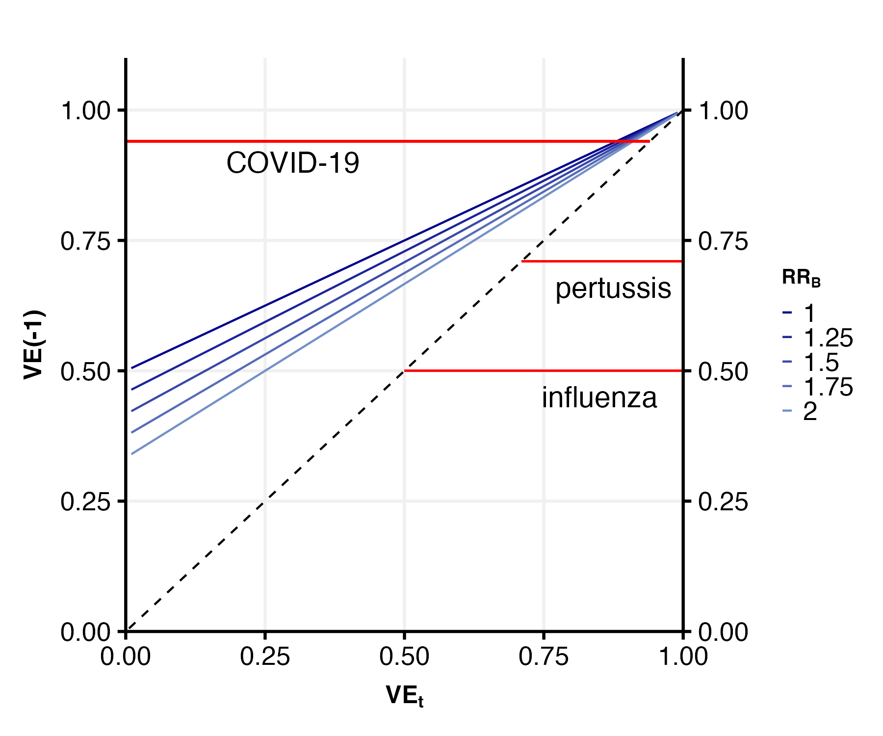
Figure 4: $VE(-1)$ versus $VE_{t}$ as a function of magnitude of broken blinding $RR_{B}$. Conventional $VE(-1)$ estimates from vaccine RCTs are added as horizontal lines.

Even when blinding is successful, such that $RR_{B}=1$, $VE(-1)$ might differ from $VE_{t}$ (Figure 4). When $RR_{B}=1$, then $VE(-1)=VE(0)=VE(1)$. When $RR_{B}>1$, $VE(-1)>VE(m)$ for $m\in\{0,1\}$, and the difference increases as $RR_{B}$ diverges from one (Web Figure 6). As $RR_{B}$ increases, $VE(-1)$ is closer to $VE_{t}$. Examples of $VE(-1)$ reported for COVID-19 [28], pertussis [46], and influenza [15] are annotated in Figure 4.

5.2 Simulations based on an influenza vaccine trial

Here we illustrate that unbiased estimation of $VE_{t}$ and $VE(m)$ for $m\in\{0,1\}$ is possible even when blinding is broken, if side effects $S$ are measured and the conditions of Proposition 2 hold. Our data-generating mechanism (DGM) is grounded in a RCT [8], comparing a seasonal influenza vaccine against saline placebo injection in children. The outcome of interest is VE against pandemic influenza A(H1N1) infection, one out of two main outcomes in the trial, coded here as a binary outcome. Our DGM is consistent with the DAG in Web Figure 7 and satisfies the published marginal proportion of adverse reactions in each treatment arm (individual-level data were not published).

The original trial was blinded and estimated $VE(-1)$ as 47%, calculated from the estimated rates $\hat{\mathbb{E}}(Y|A=0)=0.17$ and $\hat{\mathbb{E}}(Y|A=1)=0.09$. Furthermore, the trial reported that 50% of the children in the vaccine arm experienced pain or soreness of any degree at the injection site (41% mild, 8% moderate, 1%) compared to only 21% of the children in the placebo arm (19% mild, 2% moderate) [8][Table S1].

Let $S^{a}\in\{0,1\}$ indicate the presence of a side effect under $A=a$. Similar to the trial, let $\mathbb{E}(S^{a=1})=0.50$ and $\mathbb{E}(S^{a=0})=0.21$. For $m\in\{0,1\}$, let $B=m$ and for $m=-1$, let $B^{a,s,m}=B^{s}$. Furthermore, $\mathbb{E}(B^{s=1})=0.70$ and $\mathbb{E}(B^{s=0})=0.18$, reflecting that those who experience side effects are more likely to believe they received the vaccine. Under these specifications, the magnitude of different vaccine parameters differs substantially (Table 1). Further technical details about this illustration are given in Web Appendix F.

We simulated 1,000 datasets from the DGM, with sample sizes corresponding to the trial, 317 in the placebo arm and 479 in the vaccine arm. The observed data vector for each individual consisted of $(A,S,B,Y)$ and $M=-1$. To mitigate finite-sample bias, we repeated the simulations for sample sizes ten times larger (3,170 receiving placebo and 4,790 vaccine).

We estimated $VE(-1)$ by comparing infection rates for each treatment arm in each dataset, and estimated $\mathbb{E}(Y^{a,m})$ for $a,m\in\{0,1\}$ by substituting expectations with empirical means in (7). We also considered two alternative estimation strategies, where outcomes were compared across treatment arms conditional on $S=s$, for $s\in\{0,1\}$. Such strategies correspond to estimating

$$1-\frac{\mathbb{E}(Y^{a=1,m=-1}|S^{a=1,m=-1}=s)}{\mathbb{E}(Y^{a=0,m=-1}|S^{a=0,m=-1}=s)},$$

which generally does not represent a causal effect of interest. Under the assumed DAG (Web Figure 7), these strategies estimate the controlled direct effect of $A$ on $Y$, while fixing the side effects to be $s$; i.e., when comparing the joint intervention setting $A=1,M=-1,S=s$ versus the intervention $A=0,M=-1,S=s$.

The results from this DGM indicate that the mean estimates conditional on $S$, $\widehat{VE}(-1,S=0)$ and $\widehat{VE}(-1,S=1)$, are between $VE(m),m=0,1$, and and $VE(-1)$, see Table 1. In contrast, $VE_{t}$ is lower than all other VEs. For large sample sizes, our methods gave approximately unbiased estimates.

6 Discussion

Contrary to common perceptions, we have argued that the effects targeted in standard vaccine trials often differ from the effects of vaccines in real-world settings. We proposed measuring a single additional variable in a standard trial, analogous to a blinding assessment. Using this variable, and under weak assumptions, it is possible to identify effects that are often relevant to real-world vaccination programs.

To relate our results to previous work in the causal inference literature, we interpret our identification argument in the context of a six arm trial $\mathcal{T}_{VI}$. Our observed data only comprise two out of six arms in $\mathcal{T}_{VI}$, but we target parameters corresponding to expected outcomes in the unobserved four arms. Using this interpretation, $\mathcal{T}_{II}$ assigns a composite treatment $(A,M)$, where we only observe individuals with $M=-1$ deterministically. Our identification task is therefore similar to the identification task in classical separable effects settings [33, 35, 44, 42]. Inspired by the original treatment decomposition idea by Robins and Richardson [33], we have decomposed the effect of vaccination into the immunological component of the vaccine, $A$, and a deterministic message, $M=-1$. A similar story of placebo-controlled treatments was given as a motivating example for a treatment decomposition in Didelez [9], who considered interventionist mediation analysis in a survival setting. Our variable definitions are also related to, but different from, the definitions given by Murray [25], who explicitly formulated a counterfactual definition of a per-protocol placebo effect (see Web Appendix B).

Our proposal has limitations. First, our belief variable requires collection of self-reported data, which may be unreliable. As a remedy, other collected data could be used to assess blinding. As illustrated in our example, the distribution of adverse effects in the two treatment arms could indicate successful blinding. Alternatively, one could perform a negative control outcome analysis [22, 40]. Suppose, for example, that individuals in each arm of an influenza vaccine trial are tested for a panel of other, immunologically distinct respiratory infections when presenting with relevant symptoms. Comparable rates of such other infections would indicate that participants’ behavior and exposure patterns are similar across the arms.

Second, the consequences of forming a belief on behaviour might vary between diseases and populations, due to differences in risk perceptions. Future work should address such heterogeneity and assess the transportability of vaccine estimates between different settings.

Third, we defined estimands with respect to a single measurement of belief, but it is possible that beliefs change over time. Similarly, immunological effects are often time-varying, e.g. due to waning. In future extensions, we will study longitudinal settings where beliefs, exposures and outcomes vary over time. We conjecture that the methods can be generalized, under appropriate assumptions, by including a time-varying belief variable.

In conclusion, our arguments give nuance to the practical relevance of classical VE estimands. But we offer a constructive solution: different estimands, which can quantify immunological and behavioral effects of vaccination in real-world settings, can be identified and estimated under assumptions that often are plausible.

	$\mathbb{E}(Y^{1,m})$	$\mathbb{E}(Y^{0,m})$	$VE(m)$
$m=-1$	0.170	0.090	0.470
$m=0$	0.140	0.084	0.400
$m=1$	0.244	0.098	0.600

Table 1: Values of $\mathbb{E}(Y^{a,m})$ and $VE(m)$ vaccine efficacy in the simulations modelled after an influenza vaccine RCT. Under this DGM, $VE_{t}$ equals to $1-{\mathbb{E}(Y^{a=1,m=1})}/{\mathbb{E}(Y^{a=0,m=0})}=0.3$.

		Estimand
	Sample size	$VE(-1)$	$VE(0)$	$VE(1)$	$VE_{t}$	$\widehat{VE}(-1,S=0)$	$\widehat{VE}(-1,S=1)$
True value		0.47	0.40	0.60	0.30
Mean	796	0.463	0.380	0.575	0.273	0.446	0.526
	7960	0.470	0.398	0.597	0.294	0.456	0.555

Table 2: Simulation results for different estimands.

(a) DAG describing a two-arm trial $\mathcal{T}_{II}$, where $M$ is deterministically equal to $-1$. Thus, the node $M=-1$ is a trivial constant, and is only included in the graph for clarity.

(b) DAG describing the (hypothetical) four-arm trial $\mathcal{T}_{IV}$, where the bold arrow indicates the assumed determinism between the message $M$ and the belief $B$.

(c) DAG describing the hypothetical six-arm trial $\mathcal{T}_{VI}$, where $A\in\{0,1\}$ and $M\in\{-1,0,1\}$ are randomly assigned.

Figure 1: DAGs describing $\mathcal{T}_{II}$, $\mathcal{T}_{IV}$ and $\mathcal{T}_{VI}$.

Figure 2: DAG compatible with the two-arm trial $\mathcal{T}_{II}$ where $A\in\{0,1\}$ and $M=-1$. Here, Assumption 3 is expected to be violated due to the blue arrow.

Figure 3: DAG describing the six-arm trial $\mathcal{T}_{VI}$, where a side effect $S$ can affect the belief $B$. Here, the presence of the orange arrow violates Assumption 3 but not Assumption 7.

Appendix Web Appendix A

The no-interference assumption

Assumptions about no interference between individuals requires careful arguments in vaccine settings, but are often invoked and might sometimes hold. Consider for example vaccines against west Nile virus (WNV), which are currently being developed [14]. The no-interference assumption is plausible because WNV is transmitted from birds to humans, with humans having a viral load too low to carry on transmission, constituting dead-end hosts. Thus the infection of one individual, or their vaccination, should not affect the risk of infection in other individuals.

Furthermore, even when the no-interference assumption does not hold exactly in the population, this assumption might hold in the trial. Because nobody outside of the trial receives the vaccine, the only potential source of interference is among trials participants, and the trials are conducted on a small number of individuals relative to the entire population. Even the COVID-19 mRNA vaccine trials, which were large compared to most vaccine trials [28, 1], only included a small proportion of the entire population. Indeed, most analyses of vaccine RCTs rely on the no-interference assumption [47, 18].

Consider a trial of a new vaccine and let $Y_{i}^{a_{1},...,a_{n},a_{n+1},...,a_{N}}$ be the potential outcome of individual $i\in\mathcal{S}_{\text{trial}}=\{1,...,n\}$, where $\mathcal{S}_{\text{trial}}$ is the trial sample of size $n$, and $N$ is the population size. Even if the no-interference assumption does not generally hold for a specific triad of a population, disease and vaccine, it can be a reasonable assumption in a trial, as well as in the population when the proportion of vaccinated is still low. Under this particular no interference assumption,

$$Y_{i}^{a_{1},...,a_{n},a_{n+1}=0,...,a_{N}=0}=Y_{i}^{a_{i},a_{n+1}=0,...,a_{N}=0}$$

for $i\in\mathcal{S}_{\text{trial}}$, i.e., vaccination status of other trial participants $j\in\mathcal{S}_{\text{trial}},j\neq i$ is negligible. Thus, under the assumption that there is no interference in the trial, the contrast studied in the trial can be written as the direct effect of the vaccine

$$E(Y_{i}^{a_{i}=1,a_{n+1}=0,...,a_{N}=0})\text{ vs. }E(Y_{i}^{a_{i}=0,a_{n+1}=0,...,a_{N}=0}),$$ (A10)

where here the expectations are taken over $\mathcal{S}_{\text{trial}}$.

The interference in the population can be mild in some scenarios, such as shortly after a vaccination campaign has started. Then, Equation (A10) can approximate well the direct effect in the population; that is, the effect of vaccination versus non-vaccination, while fixing the vaccination status of the rest of the population. We leave more formal considerations for future work.

Therefore, the results presented in the main text distinguishing between immunological and behavioral vaccine effects can also apply for studying vaccine effects under interference. When interference is present but is negligible in the trial and in the population in the early vaccination stages, the implicit estimand in the analysis of the two-arm trial $\mathcal{T}_{II}$ is (A10) with the additional setting $m=-1$.

Appendix Web Appendix B

Per protocol effects and relation to [25]

[25] introduced a random variable $Z$ denoting treatment assignment and $X$ corresponding to received treatment, both taking values in $\{-1,0,1\}$, denoting a nontherapeutic control, placebo and active treatment, respectively. Then, intention-to-treat and per protocol effects to quantify the placebo effect were defined as

$$\mathbb{E}(Y^{z=-1})\text{ vs. }\mathbb{E}(Y^{z=0}),$$

$$\mathbb{E}(Y^{z=-1,x=-1})\text{ vs. }\mathbb{E}(Y^{z=0,x=0}).$$

To illustrate a point, consider a setting with full compliance such that the per protocol effect is equal to the intention-to-treat effect. Then, the joint of our treatments $(a=0,m=-1)$ will correspond to $(z=-1)$ and $(a=0,m=0)$ will correspond to $(z=0)$.

We can also extend our results to the setting with incomplete compliance. Let $R$ will be the treatment that is randomly assigned, which consists of our message $M$ and treatment offer $Z$ of taking treatment. Now let $A$ be the treatment (vaccine) actually taken. When the measured baseline covariates $L$ are sufficient to adjust for common causes of $A$ and $Y$, then our arguments extend to the setting in [25].

Appendix Web Appendix C

Decomposition of the total effect

In Section 3, we discussed various causal estimands, in particular the total effect (2) contrasting $\mathbb{E}(Y^{a=1,m=1})$ and $\mathbb{E}(Y^{a=0,m=0})$. Here we briefly present decompositions of such estimands, which are algebraically similar to decompositions obtained in mediation analysis [32, 27, 48].

On the difference scale,

$$\begin{split}\mathbb{E}(Y^{a=1,m=1})-\mathbb{E}(Y^{a=0,m=0})&=\big{[}\mathbb{E}(Y^{a=1,m=1})-\mathbb{E}(Y^{a=1,m=0})\big{]}+\big{[}(\mathbb{E}(Y^{a=1,m=0})-\mathbb{E}(Y^{a=0,m=0})\big{]}\\ &=\big{[}\mathbb{E}(Y^{a=1,m=1})-\mathbb{E}(Y^{a=0,m=1})\big{]}+\big{[}\mathbb{E}(Y^{a=0,m=1})-\mathbb{E}(Y^{a=0,m=0})\big{]}\end{split}$$ (C11)

so the total effect is the sum of two effects: the first line in (C11) presents the total effect as the immunological effect when $m=0$ and the behavioural effect when $a=1$; the second row decomposes the total effect into the behavioral effect without the vaccine ($A$ is held to $a=0$), and the immunological effect when $m=1$.

Analogous results are obtained on the ratio scale, where the decompositions are products rather than sums. Similar results hold for odds ratios when the outcome is rare[49].

Turning to the VE scale, under which the total VE was defined in Section 5 as $VE_{t}$, the immunological effects are $VE(m)$, and the behavioral effects (4) is $VE_{m}(a)=1-\frac{\mathbb{E}(Y^{a,m=1})}{\mathbb{E}(Y^{a,m=0})}$. Then,

$$VE_{t} =VE_{m}(0)+VE(1)-VE_{m}(0)VE(1)$$

$$=VE_{m}(1)+VE(0)-VE_{m}(1)VE(0).$$

Appendix Web Appendix D

Proofs

D.1 Proof of Proposition 1

Proof.

For $m\in\{0,1\}$, consider data from the hypothetical four-arm trial $\mathcal{T}_{IV}$, constituting four of the six-arms in the hypothetical trial $\mathcal{T}_{VI}$. We use subscripts to indicate expectations and distributions with respect to a particular trial. For example, $\mathbb{E}_{IV}(\cdot)$ is the expected value in the superpopulation of $\mathcal{T}_{IV}$. Furthermore, we assume that all participants are drawn from populations with identical distributions of all baseline and pre-baseline covariates, such that, for example $P_{IV}(L=l)=P_{VI}(L=l)=\Pr(L=l)$, where distributions without subscripts indicate the observed data from the population referring to $\mathcal{T}_{II}$.

$$\mathbb{E}(Y^{a,m}) =\mathbb{E}_{IV}(Y^{a,m})=\sum_{l}\mathbb{E}_{IV}(Y^{a,m}\mid L=l)\Pr(L=l)\text{ (LTOT)}$$

$$=\sum_{l}\mathbb{E}_{IV}(Y^{a,m}\mid M=m,A=a,L=l)\Pr(L=l)\text{ (randomization of $A$ and $M$)}$$

$$=\sum_{l}\mathbb{E}_{IV}(Y\mid M=m,A=a,L=l)\Pr(L=l)\text{ (consistency)}$$

$$=\sum_{l}\mathbb{E}_{IV}(Y\mid M=m,B=m,A=a,L=l)\Pr(L=l)\text{ ($B=M$ w.p.1 in $\mathcal{T}_{IV}$)}.$$

It follows from Assumptions 3 and 4 that the previous expression is equal to

$$\sum_{l}\mathbb{E}(Y\mid M=-1,B=m,A=a,L=l)\Pr(L=l)$$

$$=\sum_{l}\mathbb{E}(Y\mid B=m,A=a,L=l)\Pr(L=l)\text{ (Assumption \ref{ass: delta 1})},$$

which is observed in $\mathcal{T}_{II^{B}}$. ∎

D.2 Proof of Proposition 2

Proof.

For $m\in\{0,1\}$, consider data from the hypothetical four-arm trial $\mathcal{T}_{IV}$, which also constitute a subset of the data from the six-arm trial $\mathcal{T}_{VI}$.

$$\mathbb{E}(Y^{a,m})$$

$$=\mathbb{E}_{IV}(Y^{a,m})=\sum_{l}\mathbb{E}_{IV}(Y^{a,m}\mid L=l)\Pr(L=l)\text{ (LTOT)}$$

$$=\sum_{l}\mathbb{E}_{IV}(Y^{a,m}\mid M=m,A=a,L=l)\Pr(L=l)\text{ ($A,M$ randomized)}$$

$$=\sum_{l}\mathbb{E}_{IV}(Y^{a,m}\mid M=m,A=a,L=l)\Pr(L=l\mid A=a)\text{ ($A$ randomized)}$$

$$=\sum_{l}\mathbb{E}_{IV}(Y\mid M=m,A=a,L=l)\Pr(L=l\mid A=a)\text{ (consistency)}$$

$$=\sum_{l,s}\mathbb{E}_{IV}(Y\mid M=m,A=a,S=s,L=l){\Pr}_{IV}(S=s\mid L=l,A=a){\Pr}_{IV}(L=l)$$

$$\quad(\eqref{eq: delta m s},\text{ LTOT, $A$ randomized})$$

$$=\sum_{l,s}\mathbb{E}_{IV}(Y\mid M=m,B=m,A=a,S=s,L=l){\Pr}_{IV}(S=s\mid L=l,A=a){\Pr}_{IV}(L=l)\ \text{($B=M$ w.p.1)}.$$

It follows from Assumptions 7 and 8 that the previous expression is equal to

$$=\sum_{l,s}\mathbb{E}(Y\mid M=-1,B=m,A=a,S=s,L=l)\Pr(S=s,\mid L=l,A=a)\Pr(L=l)$$

$$=\sum_{l,s}\mathbb{E}(Y\mid B=m,A=a,S=s,L=l)\Pr(S=s,\mid L=l,A=a)\Pr(L=l),$$

where we also used that $A$ is randomized, that ${\Pr}_{IV}(S=s\mid L=l,A=a)=\Pr(S=s\mid L=l,A=a)$ by assumption and that $\Pr(M=-1)=1$ in $\mathcal{T}_{II}$,∎

Appendix Web Appendix E Estimation conditional on the presence of a side effect $S$

E.1 Outcome regression estimator

Consider first a simple regression estimator $\hat{\theta}_{or,a,m}$, where we define $\theta_{a,m}$ as the identification formula in Proposition 2. Let this estimator be the solution to $\sum_{i=1}^{n}U_{or,i}(\theta_{a,m},\hat{\eta})=0$ with respect to $\theta_{a,m}$, where

$$U_{or,i}(\theta_{a,m},\hat{\eta})=$$

$$\sum_{s}\mathbb{E}(Y\mid B=m,A=a,S=s,L_{i};\hat{\eta}_{1})\Pr(S=s,\mid L_{i},A=a;\hat{\eta}_{2})-\theta_{a,m}.$$

such that $\mathbb{E}(Y\mid B=m,A=a,S=s,L=l;\hat{\eta}_{1})$ and $\Pr(S=s,\mid L=l,A=a;\hat{\eta}_{2})$ are parametric models indexed by the parameter ${\eta}_{k},\ k=1,2$, where $\hat{\eta}_{k}$ is its MLE. The estimating equation defined by $U_{or,i}(\theta_{a,m},\hat{\eta})$ has mean zero and the estimator $\hat{\eta}_{or,a,m}$ is consistent provided that the models are correctly specified.

Alternatively, consider the estimator $\sum_{i=1}^{n}U^{\prime}_{or,i}(\theta_{a,m},\hat{\eta}_{1})=0$ with respect to $\theta_{a,m}$, where

$$U^{\prime}_{or,i}(\theta_{a,m},\hat{\eta}_{1})= I(A_{i}=a)\{\mathbb{E}(Y\mid B=m,A=a,S=S_{i},L=L_{i};\hat{\eta}_{1})-\theta_{a,m}\},$$

which is also consistent and requires specification of a smaller number of parametric models, but also uses less data and thus might be less efficient in the setting where all models are correctly specified.

E.2 Weighted estimator

An inverse probability weighted estimator $\hat{\theta}_{ipw,a,m}$ of $\theta_{a,m}$ is the solution to the estimating equation $\sum_{i=1}^{n}U_{ipw,i}(\theta_{a,m},\hat{\beta})=0$ with respect to $\theta_{a,m}$, where

$$U_{ipw,i}(\theta_{a,m},\hat{\beta})=\frac{I(A_{i}=a,B_{i}=m)}{\Pr(B=m\mid L=L_{i},S=S_{i},A=a;\hat{\beta}_{1})\Pr(A=a\mid L=L_{i};\hat{\beta}_{2})}\left(Y_{i}-\theta_{a,m}\right),$$

where we have indexed estimators with the parameter $\beta_{j}$ for $j\in\{1,2\}$ and assume $\hat{\beta}_{j}$ is its MLE. As stated in the main text, usually $\Pr(A=a\mid L=L_{i})=0.5$ by design in a vaccine RCT, but it can also be estimated as $\Pr(A=a\mid L=L_{i};\hat{\beta}_{2})$ for efficiency reasons.

Appendix Web Appendix F

Further details and results for the examples

F.1 Illustration of different vaccine effects

The mathematical of the DGM described in Section 5.1 of the main text is as follows. As previously noted, this illustration is presented under the graphical structure of Web Figures 5 and 5. The potential outcomes of $B$ under interventions on $A,M$ were

$$B^{a,m=0}=0,\quad\text{for}\quad a=0,1$$

$$B^{a,m=1}=1,\quad\text{for}\quad a=0,1$$

$$\mathbb{E}(B^{a=0,m=-1}=1)=0.5$$

$$\mathbb{E}(B^{a=1,m=-1}=1)=0.5\times RR_{B}$$

The potential outcomes of $Y$ under interventions on $A,M$ were

$$\begin{split}&\mathbb{E}(Y^{a=0,m=0})=0.01\\ &\mathbb{E}(Y^{a=1,m=1})=0.01\times(1-VE_{t})^{\ddagger}\\ &\mathbb{E}(Y^{a=0,m=1})=0.02^{\star}\\ &\mathbb{E}(Y^{a=1,m=0})=0.005\times(1-VE_{t})^{\star}\\ \end{split}$$ (F12)

^‡ By the definition of $VE_{t}$.
^⋆ By $\frac{\mathbb{E}(Y^{a,m=1})}{\mathbb{E}(Y^{a,m=0})}=2$ for both $a=0,1$

Under the above DGM, we can calculate $VE(m)$. We start with $VE(0)$ and $VE(1)$ which are immediately given by (LABEL:Eq:_VE_comparison_POdef) as

$$VE(0) =1-\frac{\mathbb{E}(Y^{a=1,m=0})}{\mathbb{E}(Y^{a=0,m=0})}=0.5(VE_{t}+1)$$

$$VE(1) =1-\frac{\mathbb{E}(Y^{a=1,m=1})}{\mathbb{E}(Y^{a=0,m=1})}=0.5(VE_{t}+1)$$

Turning to $VE(-1)$, note that because there are no causal and no non-casual paths between $M$ and $Y$ except the indirect effect through $B$, and because $B^{a,m}=m$ for $a,m=0,1$, we have

$$\mathbb{E}(Y^{a=0,m=-1}|B^{a=0,m=-1}=0) =\mathbb{E}(Y^{a=0,m=0}|B^{a=0,m=0}=0)=\mathbb{E}(Y^{a=0,m=0}),$$

$$\mathbb{E}(Y^{a=0,m=-1}|B^{a=0,m=-1}=1) =\mathbb{E}(Y^{a=0,m=1}|B^{a=0,m=1}=1)=\mathbb{E}(Y^{a=0,m=1}),$$

$$\mathbb{E}(Y^{a=1,m=-1}|B^{a=1,m=-1}=1) =\mathbb{E}(Y^{a=1,m=1}|B^{a=0,m=1}=1)=\mathbb{E}(Y^{a=1,m=1}),$$

$$\mathbb{E}(Y^{a=1,m=-1}|B^{a=1,m=-1}=0) =\mathbb{E}(Y^{a=1,m=0}|B^{a=1,m=0}=0)=\mathbb{E}(Y^{a=1,m=0}).$$

We can now use the above results to derive $\mathbb{E}(Y^{a=0,m=-1})$ and $\mathbb{E}(Y^{a=1,m=-1})$, as follows.

$$\mathbb{E} (Y^{a=0,m=-1})$$

$$=\mathbb{E}(Y^{a=0,m=-1}|B^{a=0,m=-1}=1)\times 0.5+\mathbb{E}(Y^{a=0,m=-1}|B^{a=0,m=-1}=0)\times 0.5$$

$$=\mathbb{E}(Y^{a=0,m=1})\times 0.5+\mathbb{E}(Y^{a=0,m=0})\times 0.5$$

$$=0.03\times 0.5=0.015.$$

Next,

$$\mathbb{E} (Y^{a=1,m=-1})$$

$$=\mathbb{E}(Y^{a=1,m=-1}|B^{a=1,m=-1}=1)\times 0.5\times RR_{B}+\mathbb{E}(Y^{a=1,m=-1}|B^{a=1,m=-1}=0)\times(1-0.5RR_{B})$$

$$=\mathbb{E}(Y^{a=1,m=1})\times 0.5\times RR_{B}+\mathbb{E}(Y^{a=1,m=0})\times(1-0.5\times RR_{B})$$

$$=0.01\times(1-VE_{t})\times 0.5\times RR_{B}+0.005\times(1-VE_{t})\times(1-0.5\times RR_{B})$$

$$=(1-VE_{t})\times(0.005+0.0025\times RR_{B}).$$

Therefore,

$$VE(-1)=1-\frac{(1-VE_{t})\times(0.005+0.0025\times RR_{B})}{0.015}$$

(a) DAG describing the two-arm trial $\mathcal{T}_{II}$ from Section 5.1, where $M$ is deterministically equal to $-1$. Thus, the node $M=-1$ is a trivial constant, and is only included for clarity.

(b) DAG describing the six-arm trial $\mathcal{T}_{VI}$ from Section 5.1. The arrows from $M$ and $A$ to $B$ reflect that when $M=0,1$, then $B=M$, and when $M=-1$, then $B$ is a random variable whose distribution depends on $A$.

Web Figure 5: Figures describing the DGM used in Section 5.1.

Web Figure 6 presents an additional comparison, between $VE(-1)$ as a function of $VE(0)=VE(1)$ for different $RR_{B}$ values and the relationship between $VE_{t}$ and $VE(0)=VE(1)$. Because it is assumed a message $M=1$ induces more risky behaviour, we obtained that $VE_{t}<VE(m),m=0,1$.

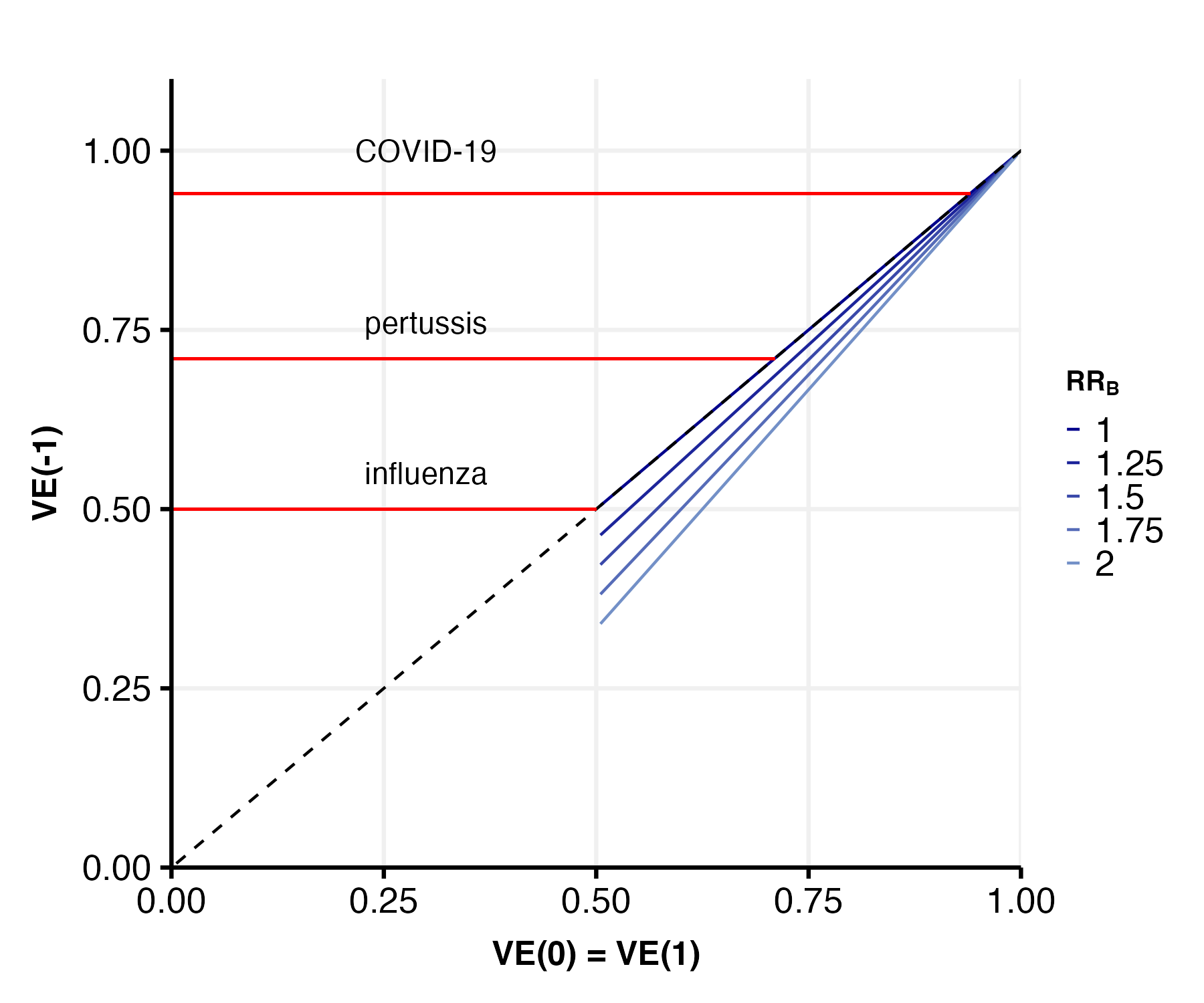
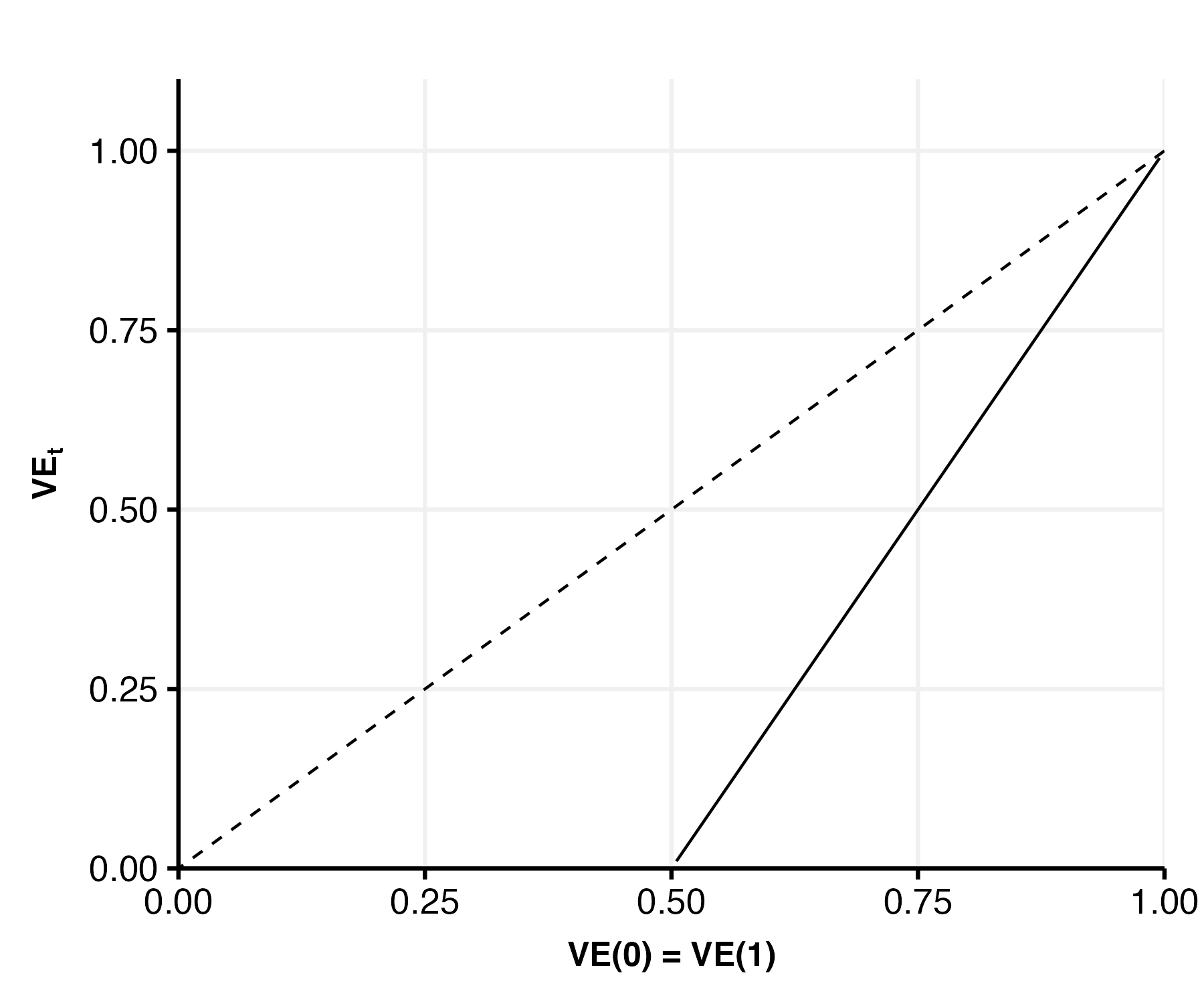
Web Figure 6: $VE(-1)$ and $VE_{t}$ as a function of $VE(m),m=0,1$ for different $RR_{B}$ values. Note that $VE(m),m=0,1$ and $VE_{t}$ are not functions of $RR_{B}$, because the belief is identical to the message in these comparisons.

F.2 Simulations

Web Figure 7 describes the assumptions underlying the DGM used in our simulations. Starting from the non-trial conditions ($A=M=B$), $\mathbb{E}(Y^{a,m})$ are determined by setting $\mathbb{E}(Y^{a=0,m=0})$, $VE_{t}$, and $VE(m)$ for $m=0,1$. The values will be determined later to obtain similar results to the trial. Next, to calculate $\mathbb{E}(Y^{a,m=-1})$, we note that for $m=-1$, only $S$ affects $B$, and we can write

$$\mathbb{E} (Y^{a,m=-1})$$

$$=\mathbb{E} (Y^{a,m=-1}|B^{s=0,m=-1}=1,S^{a=1}=0)\Pr(S^{a}=0)\Pr(B^{s=0,m=-1}=1)$$

$$+\mathbb{E}(Y^{a,m=-1}|B^{s=1,m=-1}=1,S^{a=1}=1)\Pr(S^{a}=1)\Pr(B^{s=1,m=-1}=1)$$

$$+\mathbb{E}(Y^{a,m=-1}|B^{s=0,m=-1}=0,S^{a=1}=0)\Pr(S^{a}=0)\Pr(B^{s=0,m=-1}=0)$$

$$+\mathbb{E}(Y^{a,m=-1}|B^{s=1,m=-1}=0,S^{a=1}=1)\Pr(S^{a}=1)\Pr(B^{s=1,m=-1}=0)$$

$$=\mathbb{E} (Y^{a,m=1})\big{[}\Pr(S^{a}=0)\Pr(B^{s=0}=1)+\Pr(S^{a}=1)\Pr(B^{s=1}=1)\big{]}$$

$$+\mathbb{E}(Y^{a,m=0})\big{[}\Pr(S^{a}=0)\Pr(B^{s=0}=0)+\Pr(S^{a}=1)\Pr(B^{s=1}=0)\big{]}$$

Note these weights can be abbreviated a bit recognizing it’s just the probability of belief Now, under the values given below, we obtain population-level results similar to what was obtained in the trial. We took $\mathbb{E}(Y^{a,m=-1})$ (and therefore $VE(-1)$) to be approximately equal to $\hat{\Pr}(Y=1|A=a)$ from the trial. The estimated VE in the trial was 0.47. We also took the probability of side effects under each treatment $\Pr(S^{a}=1)$ to be equal to the trial observed proportions of soreness of any severity at each treatment arm. We took

$$\mathbb{E}(Y^{a=0,m=-1}) =0.170$$

$$\mathbb{E}(Y^{a=1,m=-1}) =0.090$$

$$\mathbb{E}(Y^{a=0,m=0}) =0.1395$$

$$VE_{tot} =0.3$$

$$VE(0) =0.40$$

$$VE(1) =0.60$$

$$\Pr(S^{a=1}=1) =0.50$$

$$\Pr(S^{a=0}=1) =0.21$$

$$\Pr(B^{s=1}=1) =0.70$$

$$\Pr(B^{s=0}=1) =0.18$$

which resulted in the mean potential outcomes $\mathbb{E}(Y^{a,m})$ given in Table 1 of the main text.

Web Figure 7: DAG describing the simulations according to a six-arm trial $\mathcal{T}_{VI}$, where a side effect $S$ can affect the belief $B$.

References

- Baden et al. [2021] L. R. Baden, H. M. El Sahly, B. Essink, K. Kotloff, S. Frey, R. Novak, D. Diemert, S. A. Spector, N. Rouphael, C. B. Creech, et al. Efficacy and safety of the mrna-1273 sars-cov-2 vaccine. New England journal of medicine, 384(5):403–416, 2021.
- Beedie et al. [2006] C. J. Beedie, E. M. Stuart, D. A. Coleman, A. J. Foad, et al. Placebo effects of caffeine on cycling performance. Medicine and science in sports and exercise, 38(12):2159, 2006.
- Bello et al. [2014] S. Bello, H. Moustgaard, and A. Hróbjartsson. The risk of unblinding was infrequently and incompletely reported in 300 randomized clinical trial publications. Journal of clinical epidemiology, 67(10):1059–1069, 2014.
- Bender et al. [2022] F. Bender, W. Rief, and M. Wilhelm. Really just a little prick? a meta-analysis on adverse events in placebo control groups of seasonal influenza vaccination rcts. Vaccine, 2022.
- Boutron et al. [2005] I. Boutron, C. Estellat, and P. Ravaud. A review of blinding in randomized controlled trials found results inconsistent and questionable. Journal of clinical epidemiology, 58(12):1220–1226, 2005.
- Brewer et al. [2007] N. T. Brewer, C. L. Cuite, J. E. Herrington, and N. D. Weinstein. Risk compensation and vaccination: can getting vaccinated cause people to engage in risky behaviors? Annals of Behavioral Medicine, 34(1):95, 2007.
- Colagiuri [2010] B. Colagiuri. Participant expectancies in double-blind randomized placebo-controlled trials: potential limitations to trial validity. Clinical Trials, 7(3):246–255, 2010.
- Cowling et al. [2012] B. J. Cowling, S. Ng, E. S. Ma, V. J. Fang, H. C. So, W. Wai, C. K. Cheng, J. Y. Wong, K.-H. Chan, D. K. Ip, et al. Protective efficacy against pandemic influenza of seasonal influenza vaccination in children in hong kong: a randomized controlled trial. Clinical Infectious Diseases, 55(5):695–702, 2012.
- Didelez [2018] V. Didelez. Defining causal meditation with a longitudinal mediator and a survival outcome. Lifetime data analysis, pages 1–18, 2018.
- Ejelöv and Luke [2020] E. Ejelöv and T. J. Luke. “rarely safe to assume”: Evaluating the use and interpretation of manipulation checks in experimental social psychology. Journal of Experimental Social Psychology, 87:103937, 2020.
- Fisher and Greenberg [1993] S. Fisher and R. P. Greenberg. How sound is the double-blind design for evaluating psychotropic drugs? The Journal of nervous and mental disease, 181(6):345–350, 1993.
- Freed et al. [2021] B. Freed, B. Williams, X. Situ, V. Landsman, J. Kim, A. Moroz, H. Bang, and J. J. Park. Blinding, sham, and treatment effects in randomized controlled trials for back pain in 2000–2019: a review and meta-analytic approach. Clinical Trials, 18(3):361–370, 2021.
- Goldszmidt et al. [2021] R. Goldszmidt, A. Petherick, E. B. Andrade, T. Hale, R. Furst, T. Phillips, and S. Jones. Protective behaviors against covid-19 by individual vaccination status in 12 countries during the pandemic. JAMA Network Open, 4(10):e2131137–e2131137, 2021.
- Gould et al. [2023] C. V. Gould, J. E. Staples, C. Y.-H. Huang, A. C. Brault, and R. J. Nett. Combating west nile virus disease—time to revisit vaccination. New England Journal of Medicine, 2023.
- Govaert et al. [1994] T. M. Govaert, C. Thijs, N. Masurel, M. Sprenger, G. Dinant, and J. Knottnerus. The efficacy of influenza vaccination in elderly individuals: a randomized double-blind placebo-controlled trial. Jama, 272(21):1661–1665, 1994.
- Haas et al. [2022] J. W. Haas, F. L. Bender, S. Ballou, J. M. Kelley, M. Wilhelm, F. G. Miller, W. Rief, and T. J. Kaptchuk. Frequency of adverse events in the placebo arms of covid-19 vaccine trials: a systematic review and meta-analysis. JAMA network open, 5(1):e2143955–e2143955, 2022.
- Hall et al. [2022] P. A. Hall, G. Meng, M. N. Sakib, A. C. Quah, T. Agar, and G. T. Fong. Do the vaccinated perform less distancing, mask wearing and hand hygiene? a test of the risk compensation hypothesis in a representative sample during the covid-19 pandemic. Vaccine, 2022.
- Halloran et al. [1996] M. E. Halloran, I. M. Longini Jr, and C. J. Struchiner. Estimability and interpretation of vaccine efficacy using frailty mixing models. American Journal of Epidemiology, 144(1):83–97, 1996.
- Hossain et al. [2022] M. E. Hossain, M. S. Islam, M. J. Rana, M. R. Amin, M. Rokonuzzaman, S. Chakrobortty, and S. M. Saha. Scaling the changes in lifestyle, attitude, and behavioral patterns among covid-19 vaccinated people: insights from bangladesh. Human Vaccines & Immunotherapeutics, 18(1):2022920, 2022.
- Hróbjartsson et al. [2007] A. Hróbjartsson, E. Forfang, M. Haahr, B. Als-Nielsen, and S. Brorson. Blinded trials taken to the test: an analysis of randomized clinical trials that report tests for the success of blinding. International journal of epidemiology, 36(3):654–663, 2007.
- Kahan et al. [2015] B. C. Kahan, S. Rehal, and S. Cro. Blinded outcome assessment was infrequently used and poorly reported in open trials. PloS one, 10(6):e0131926, 2015.
- Lipsitch et al. [2010] M. Lipsitch, E. T. Tchetgen, and T. Cohen. Negative controls: a tool for detecting confounding and bias in observational studies. Epidemiology (Cambridge, Mass.), 21(3):383, 2010.
- Moscucci et al. [1987] M. Moscucci, L. Byrne, M. Weintraub, and C. Cox. Blinding, unblinding, and the placebo effect: An analysis of patients’ guesses of treatment assignment in a double-blind clinical trial. Clinical Pharmacology & Therapeutics, 41(3):259–265, 1987.
- Moustgaard et al. [2020] H. Moustgaard, G. L. Clayton, H. E. Jones, I. Boutron, L. Jørgensen, D. R. Laursen, M. F. Olsen, A. Paludan-Müller, P. Ravaud, J. Savović, et al. Impact of blinding on estimated treatment effects in randomised clinical trials: meta-epidemiological study. bmj, 368, 2020.
- Murray [2021] E. J. Murray. Demystifying the placebo effect. American Journal of Epidemiology, 190(1):2–9, 2021.
- Pandit et al. [2022] J. A. Pandit, J. M. Radin, G. Quer, and E. J. Topol. Smartphone apps in the covid-19 pandemic. Nature Biotechnology, 40(7):1013–1022, 2022.
- Pearl [2001] J. Pearl. Direct and indirect effects. In Proceedings of the seventeenth conference on uncertainty in artificial intelligence, pages 411–420. Morgan Kaufmann Publishers Inc., 2001.
- Polack et al. [2020] F. P. Polack, S. J. Thomas, N. Kitchin, J. Absalon, A. Gurtman, S. Lockhart, J. L. Perez, G. Pérez Marc, E. D. Moreira, C. Zerbini, et al. Safety and efficacy of the bnt162b2 mrna covid-19 vaccine. New England journal of medicine, 383(27):2603–2615, 2020.
- Polit et al. [2011] D. F. Polit, B. M. Gillespie, and R. Griffin. Deliberate ignorance: a systematic review of blinding in nursing clinical trials. Nursing research, 60(1):9–16, 2011.
- Rid et al. [2014] A. Rid, A. Saxena, A. H. Baqui, A. Bhan, J. Bines, M.-C. Bouesseau, A. Caplan, J. Colgrove, A. Dhai, R. Gomez-Diaz, et al. Placebo use in vaccine trials: recommendations of a who expert panel. Vaccine, 32(37):4708–4712, 2014.
- Robins [1986] J. M. Robins. A new approach to causal inference in mortality studies with a sustained exposure period—application to control of the healthy worker survivor effect. Mathematical modelling, 7(9-12):1393–1512, 1986.
- Robins and Greenland [1992] J. M. Robins and S. Greenland. Identifiability and exchangeability for direct and indirect effects. Epidemiology, pages 143–155, 1992.
- Robins and Richardson [2010] J. M. Robins and T. S. Richardson. Alternative graphical causal models and the identification of direct effects. Causality and psychopathology: Finding the determinants of disorders and their cures, pages 103–158, 2010.
- Robins et al. [2000] J. M. Robins, M. A. Hernan, and B. Brumback. Marginal structural models and causal inference in epidemiology, 2000.
- Robins et al. [2020] J. M. Robins, T. S. Richardson, and I. Shpitser. An interventionist approach to mediation analysis. arXiv preprint arXiv:2008.06019, 2020.
- Roscoe et al. [2010] J. A. Roscoe, M. O’Neill, P. Jean-Pierre, C. E. Heckler, T. J. Kaptchuk, P. Bushunow, M. Shayne, A. Huston, R. Qazi, and B. Smith. An exploratory study on the effects of an expectancy manipulation on chemotherapy-related nausea. Journal of pain and symptom management, 40(3):379–390, 2010.
- Schnoll et al. [2008] R. A. Schnoll, L. Epstein, J. Audrain, R. Niaura, L. Hawk, P. G. Shields, C. Lerman, and E. P. Wileyto. Can the blind see? participant guess about treatment arm assignment may influence outcome in a clinical trial of bupropion for smoking cessation. Journal of substance abuse treatment, 34(2):234–241, 2008.
- Scott et al. [2022] A. J. Scott, L. Sharpe, and B. Colagiuri. A systematic review and meta-analysis of the success of blinding in antidepressant rcts. Psychiatry Research, 307:114297, 2022.
- Serisier et al. [2023] A. Serisier, S. Beale, Y. Boukari, S. Hoskins, V. Nguyen, T. Byrne, W. L. E. Fong, E. Fragaszy, C. Geismar, J. Kovar, et al. A case-crossover study of the effect of vaccination on sars-cov-2 transmission relevant behaviours during a period of national lockdown in england and wales. Vaccine, 41(2):511–518, 2023.
- Shi et al. [2020] X. Shi, W. Miao, and E. T. Tchetgen. A selective review of negative control methods in epidemiology. Current epidemiology reports, 7:190–202, 2020.
- Stensrud and Smith [2022] M. J. Stensrud and L. Smith. Identification of vaccine effects when exposure status is unknown. Epidemiology, 34(2):216–224, 2022.
- Stensrud et al. [2020] M. J. Stensrud, J. G. Young, V. Didelez, J. M. Robins, and M. A. Hernán. Separable effects for causal inference in the presence of competing events. Journal of the American Statistical Association, pages 1–9, 2020.
- Stensrud et al. [2021] M. J. Stensrud, M. A. Hernán, E. J. Tchetgen Tchetgen, J. M. Robins, V. Didelez, and J. G. Young. A generalized theory of separable effects in competing event settings. Lifetime Data Analysis, pages 1–44, 2021.
- Stensrud et al. [2022] M. J. Stensrud, J. M. Robins, A. Sarvet, E. J. Tchetgen Tchetgen, and J. G. Young. Conditional separable effects. Journal of the American Statistical Association, pages 1–13, 2022.
- Thorpe et al. [2022] A. Thorpe, A. Fagerlin, F. Drews, H. Shoemaker, and L. Scherer. Self-reported health behaviors and risk perceptions following the covid-19 vaccination rollout in the usa: an online survey study. Public Health, 208:68–71, 2022.
- Trollfors et al. [1995] B. Trollfors, J. Taranger, T. Lagergård, L. Lind, V. Sundh, G. Zackrisson, C. U. Lowe, W. Blackwelder, and J. B. Robbins. A placebo-controlled trial of a pertussis-toxoid vaccine. New England Journal of Medicine, 333(16):1045–1050, 1995.
- Tsiatis and Davidian [2021] A. A. Tsiatis and M. Davidian. Estimating vaccine efficacy over time after a randomized study is unblinded. arXiv preprint arXiv:2102.13103, 2021.
- VanderWeele [2015] T. VanderWeele. Explanation in causal inference: methods for mediation and interaction. Oxford University Press, 2015.
- VanderWeele and Vansteelandt [2010] T. J. VanderWeele and S. Vansteelandt. Odds ratios for mediation analysis for a dichotomous outcome. American journal of epidemiology, 172(12):1339–1348, 2010.
- Webster et al. [2021] R. K. Webster, F. Bishop, G. S. Collins, A. W. Evers, T. Hoffmann, J. A. Knottnerus, S. E. Lamb, H. Macdonald, C. Madigan, V. Napadow, et al. Measuring the success of blinding in placebo-controlled trials: Should we be so quick to dismiss it? Journal of Clinical Epidemiology, 135:176–181, 2021.
- Wright et al. [2022] L. Wright, A. Steptoe, H. W. Mak, and D. Fancourt. Do people reduce compliance with covid-19 guidelines following vaccination? a longitudinal analysis of matched uk adults. J Epidemiol Community Health, 76(2):109–115, 2022.