Radio Galaxy Zoo: Leveraging latent space representations from variational autoencoder

Abstract

We propose to learn latent space representations of radio galaxies, and train a very deep variational autoencoder (VDVAE) on RGZ DR1, an unlabeled dataset, to this end. We show that the encoded features can be leveraged for downstream tasks such as classifying galaxies in labeled datasets, and similarity search. Results show that the model is able to reconstruct its given inputs, capturing the salient features of the latter. We use the latent codes of galaxy images, from MiraBest Confident and FR-DEEP NVSS datasets, to train various non-neural network classifiers. It is found that the latter can differentiate FRI from FRII galaxies achieving accuracy $\geq 76\%$, roc-auc $\geq 0.86$, specificity $\geq 0.73$ and recall $\geq 0.78$ on MiraBest Confident dataset, comparable to results obtained in previous studies. The performance of simple classifiers trained on FR-DEEP NVSS data representations is on par with that of a deep learning classifier (CNN based) trained on images in previous work, highlighting how powerful the compressed information is. We successfully exploit the learned representations to search for galaxies in a dataset that are semantically similar to a query image belonging to a different dataset. Although generating new galaxy images (e.g. for data augmentation) is not our primary objective, we find that the VDVAE model is a relatively good emulator. Finally, as a step toward detecting anomaly/novelty, a density estimator – Masked Autoregressive Flow (MAF) – is trained on the latent codes, such that the log-likelihood of data can be estimated. The downstream tasks conducted in this work demonstrate the meaningfulness of the latent codes.

1 Introduction

Galaxy morphology is a powerful probe for investigating galaxy evolutionary processes, e.g. star formation history, the physical processes that galaxies undergo in their environment. Surveys like DESI [1] and SDSS [2, 3], which make tens of millions of galaxy images available, provide insights into galaxy formation and evolution. On the radio counterpart, a great deal of effort has been made toward building datasets of radio galaxy images, e.g. Radio Galaxy Zoo [4], and upcoming large experiments like SKA [5, 6] will increase the amount of data available. Most of the methods that have been considered to identify galaxies with different morphological features are supervised learning based, which heavily relies on labeling of the data. So far, they have been successful, although manual labeling process is not only expensive but could also potentially introduce biases in the data. Morever, for new scientific discoveries and searching for anomalies in large uncurated datasets, resorting to the feature extractors that are trained in a supervised learning setup is not optimal due to the fact that they are not robust to both noise and dataset shift.

Self-supervised learning (SSL) [7, 8, 9, 10], which does not require data labeling, has been considered to uncover patterns in unlabeled dataset by learning robust representations of the high dimensional images. For example, [11] successfully used constrastive learning to search for galaxies that are semantically similar in large datasets. [12] considered SimCLR method [13] to learn representations of astronomical images from SDSS, and [14] opted for Boostrap Your Own Latent (BYOL) method [8] to extract important features of radio galaxies.

In this work, we aim to learn latent codes of radio galaxies using a generative model, Very Deep Variational AutoEncoder (VDVAE). Earlier work [15] used VAE, whose both encoder and decoder were composed of only fully connected layers, to generate synthetic images of Fanaroff-Riley Class I (FRI) and Class II (FRII) radio galaxies. Their approach was capable of generating realistic radio galaxy images, but the generated and reconstructed images were blurry, which could be attributed to the lack of expressivity of the network. Our main goal in this work, unlike the case studied in [15], is to highlight the ability of a deep generative model, VDVAE, to learn meaningful representations which can be leveraged for various downstream tasks. We also show how to estimate the log-likelihood of data using the learned representations, which is useful within the context of anomaly/novelty detection. We present the datasets used in our analyses in Section 2, and introduce the model considered in this study and other SSL based methods used for comparison in Section 3. The main results and the data likelihood estimation are reported in Sections 4 and 5 respectively, and we conclude in Section 6.

2 Data

We make use of the Radio Galaxy Zoo Data Release 1 (RGZ DR1) (Wong et al. 2023 in prep) to train and evaluate our generative model. The dataset used in our analyses contains $\sim 100,000$ unlabeled galaxies with their corresponding projected angular size in arcseconds. The input image to our model has a selected resolution of $64\times 64$ pixels.
To investigate the ability of our network, and that of other SSL based methods used for comparison in our analyses, to compress the images, we train various non-neural network methods on the latent features of galaxy images from two different datasets, MiraBest Confident dataset (MBC)[16, 17, 18] and FR-DEEP NVSS dataset [19]. The idea is to identify FRI and FRII galaxy images in each dataset by only exploiting their representations. MBC and FR-DEEP NVSS have 729/104 (train/test) and 550/50 (train/test) instances respectively, and their images are also cropped to $64\times 64$ pixels. The numbers of FRI and FRII in the training examples are roughly equal in both datasets, with an imbalance ratio $\sim 0.5$. It is worth noting that the RGZ DR1 contains some MBC samples which are flagged out when training the feature extractors.

3 Models

In our investigation, we also train various SSL based methods and compare their performance with that of our network, specifically in terms of using the encoded features to identify galaxy types in labeled datasets, MBC and FR-DEEP NVSS. In this section we provide the technical details of each algorithm together with the hyperparameters selected to train them.

3.1 Very deep variational autoencoder (VDVAE)

Variational autoencoder (VAE) [20] is a type of generative model that is composed of an encoder $q_{\phi}(\bm{z}|\bm{x})$ – which is an approximate posterior given the intractability of the true posterior –, a decoder $p_{\theta}(\bm{x}|\bm{z})$ and a prior $p_{\theta}(\bm{z})$. The two networks $\phi$ and $\theta$ are simultaneously trained by maximizing the evidence lower bound ($\mathbb{ELBO}$)

$$\mathbb{ELBO}=E_{\bm{z}\sim q_{\phi}(\bm{z}|\bm{x})}{\rm log}p_{\theta}(\bm{x}|\bm{z})-D_{KL}(q_{\phi}(\bm{z}|\bm{x})||p_{\theta}(\bm{z})),$$ (3.1)

where the first term denotes the reconstruction error which measures how well the model recovers the inputs, and the second term is the Kullback-Leibler (KL) divergence, quantifying the dissimilarity between $q_{\phi}(\bm{z}|\bm{x})$ and $p_{\theta}(\bm{z})$.

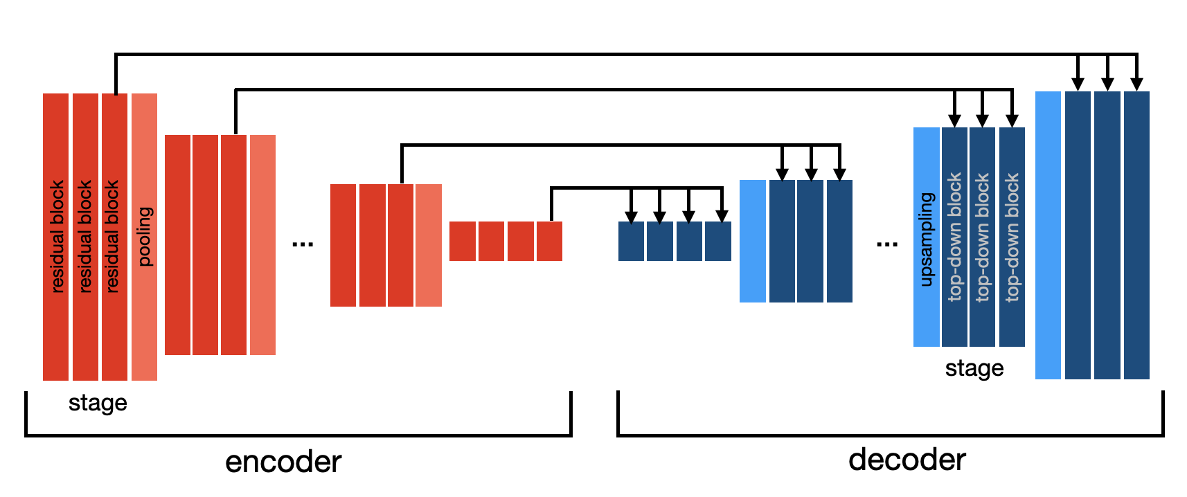
Figure 1: Schematic diagram of the VDVAE— model. The red and blue blocks denote the residual blocks of the encoder and top-down blocks of the decoder respectively. The black arrows indicate mixing via concatenation along the channel dimension.

It is worth noting that VAE outputs (either reconstructed or generated images) are known to suffer from blurriness, which can be potentially mitigated by controlling the contribution of the KL divergence to the total loss, using a hyperparameter $\beta$ according to [21]

$$\mathbb{ELBO}=E_{\bm{z}\sim q_{\phi}(\bm{z}|\bm{x})}{\rm log}p_{\theta}(\bm{x}|\bm{z})-\beta D_{KL}(q_{\phi}(\bm{z}|\bm{x})||p_{\theta}(\bm{z})).$$ (3.2)

There are several variants of the VAE models but we consider the Very Deep Variational Autoencoder (VDVAE) model prescribed by [22] in our analyses. In order to increase the expressivity of both the prior $p_{\theta}(\bm{z})$ and approximate posterior $q_{\phi}(\bm{z}|\bm{x})$, [22] proposed a hierarchical VAE comprising many stochastic layers of latent variables. The latter have different resolutions $\bm{z}_{0},\bm{z}_{1},...,\bm{z}_{N}$ which are conditionally dependent on each other according to

$$p_{\theta}(\bm{z})=p_{\theta}(\bm{z}_{0})\prod_{k=1}^{N}p_{\theta}(\bm{z}_{k}|\bm{z}_{k-1}),$$

$$q_{\phi}(\bm{z}|\bm{x})=q_{\phi}(\bm{z}_{0}|\bm{x})\prod_{k=1}^{N}q_{\phi}(\bm{z}_{k}|\bm{z}_{k-1},\bm{x}),$$ (3.3)

where $N$ is the number of layers, and the conditionals $q_{\phi}(\cdot)$ and $p_{\theta}(\cdot)$ are parameterized as diagonal Gaussians. In this work, we consider the latent variable with the lowest resolution $\bm{z}_{0}$ which is a vector of length 256, i.e. a feature vector with 256 components. Figure 1 presents a schematic diagram of the model architecture. A residual block, which comprises 4 convolutional layers, is an important component of the two networks $\phi$ and $\theta$. The encoder contains multiple stages which are built by stacking residual blocks (see red blocks in Figure 1). The output of one stage is downsampled by using average pooling. Each stage of the decoder is composed of chained top-down blocks. At the level of each top-down block, the prior, the posterior and the latent variable are computed by using one residual block, another residual block and one convolutional layer respectively; and a third residual block is used at the output. The feature maps outputted by the last top-down block at a given stage is upsampled using nearest neighbor method. It is noted that both networks ($\phi$ and $\theta$) have the same number of stages and the dimensions of feature maps from two corresponding stages are the same. The input of each top-down block of the decoder at a given stage is concatenated with the output of the last residual block at the corresponding stage of the encoder (see Figure 1). The augmented feature maps resulting from this mixing are used to compute the conditionals $q_{\phi}(\cdot)$ and $p_{\theta}(\cdot)$ in Equation 3.1. The encoder and decoder have 6 stages of $\{3,3,2,2,2,1\}$ residual blocks and $\{5,5,4,3,2,1\}$ top-down blocks respectively. The decoder is chosen to be a bit deeper for good quality of generated images. Our choice might be suboptimal but good enough for our purpose. We consider RMSProp optimizer with a learning rate of 0.00002, momentum set to 0.9, and weight decay of 0.0001. We train the model for 100 epochs with batch size of 32. The learning rate is reduced by a factor 0.5 whenever the validation loss does not improve over 10 epochs during training, i.e. using ReduceLROnPlateau scheduler. We mainly follow the parameters in [22] with some adjustments due to computing resources.

3.2 SimCLR method

Contrastive learning method consists of minimizing the distance between two different augmentations of an image in latent space while increasing distance between representations of augmented views of different images, i.e. in latent space, an image and its transformations are clustered, and pushed away from other images and their corresponding augmentations.

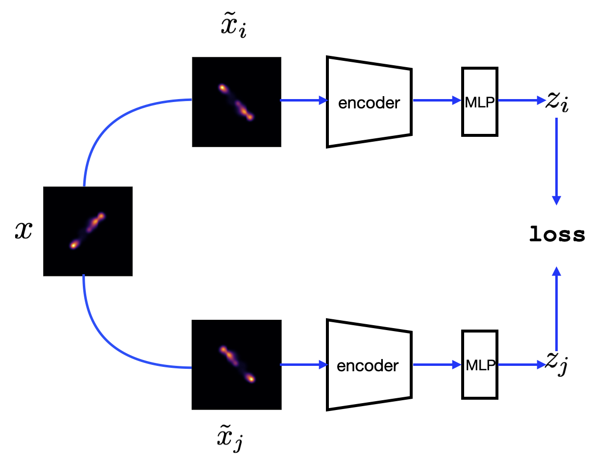
Figure 2: Schematic diagram of SimCLR— method.

In this work we consider SimCLR method [7] which applies two stochastic transformations to an image, resulting in two different augmented views $\tilde{\bm{x}}_{i}$ and $\tilde{\bm{x}}_{j}$ which form a positive pair $\{\tilde{\bm{x}}_{i},\tilde{\bm{x}}_{j}\}$. The corresponding features of the latter – $\bm{h}_{i}$ and $\bm{h}_{j}$ respectively – are extracted via an encoder. Finally, the representations $\{\bm{h}_{i}$, $\bm{h}_{j}\}$ are projected into latent space using a multilayer perceptron (MLP), giving $\{\bm{z}_{i},\bm{z}_{j}\}$ as shown in Figure 2. The separation of positive pairs $\{\bm{z}_{i},\bm{z}_{j}\}$ in latent space is minimized while that of negative pairs is maximized using a constrastive loss, also known as NT-Xent (normalized temperature-scaled cross entropy loss) [23, 7]

$$\ell(i,j)=-{\rm log}\frac{{\rm exp}({\rm sim}(\bm{z}_{i},\bm{z}_{j})/\tau)}{\sum_{k=1}^{2N}\mathbbm{1}_{[k\neq i]}{\rm exp}({\rm sim}(\bm{z}_{i},\bm{z}_{k})/\tau)},$$ (3.4)

where $\mathbbm{1}_{[k\neq i]}$ is equal to 1, 0 if and only if $k\neq i$ (for negative pairs) and $k=i$ respectively, and $\tau$ is known as the temperature parameter. The function ${\rm sim}(\bm{z}_{i},\bm{z}_{j})$ denotes cosine similarity ${\rm sim}(\bm{z}_{i},\bm{z}_{j})=\bm{z}_{i}\cdot\bm{z}_{j}/(||\bm{z}_{i}||\>||\bm{z}_{j}||)$. In our case, the stochastic transformation is defined by a set of data augmentations which are a random horizontal flip, a random vertical flip, a random crop, a random color jitter, and a Gaussian blur. We make use of Resnet-34 [24] as a backbone. The model is trained for 1000 epochs, using LARS optimizer with a learning rate lr = 0.001 and a batch of 1024 instances. The encoded features which are arrays of length 512 are projected into latent space using an MLP with one hidden layer, yielding vectors with 128 components.

3.3 BYOL method

In order to avoid collapsed representations, constrastive methods such as SimCLR learn to distinguish representations of distorted views of an image from those of different images, and

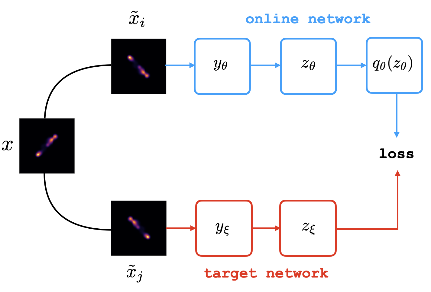
Figure 3: Schematic diagram of BYOL— method. The online network components are shown in blue, whereas those of the target are in red.

the representations learned by SimCLR are of better quality with larger batches during training [7]. Unlike SimCLR, BYOL method [8] bypasses the need for negative examples, but rather uses an online network that learns to predict the outputs of a target network (Figure 3). The former, defined by its parameters $\theta$, comprises an encoder that outputs a representation $y_{\theta}$ which, similar to the case of SimCLR, is projected into latent space $z_{\theta}$. To avoid collapsing results, a predictor $q_{\theta}(z_{\theta})$, which processes $z_{\theta}$, is added to the online network (see Figure 3). The target network architecture is a copy of that of the online but its weights $\xi$ are computed from an exponential average of $\theta$ at each training step according to

$$\xi\longleftarrow\kappa\xi+(1-\kappa)\theta,$$ (3.5)

where $\kappa$ indicates the decay rate $\in$ [0, 1]. In other words, the gradients related to target parameters are not computed. Two augmented views, obtained from stochastic transformations, of an image $\tilde{\bm{x}_{i}}$ and $\tilde{\bm{x}_{j}}$ are passed through the online and target pipelines (see Figure 3) respectively, and the online network is trained to predict the target $z_{\xi}$, resulting in refined representations. This boostrapping procedure helps the online network improve the quality of its learned representations as the training progresses. The loss is defined by a mean squared error between the target projection and the online prediction [8]

$$\mathcal{L}=||q_{\theta}(z_{\theta})-z_{\xi}||^{2}_{2}.$$ (3.6)

We also consider Resnet-34 as backbone, and opt for LARS optimizer with learning rate of $0.0005$, batch of 1024 examples and training epochs of 1000. Both online projector and predictor consist of one hidden layer MLP. The set of data augmentations considered during training is the same as the one for SimCLR.

3.4 SimSiam method

SimSiam [10] rejects the need for a momentum encoder and negative examples altogether to prevent collapsing results. Like SimCLR, the parameters are shared between the two pipelines (blue and red branches in Figure 4),

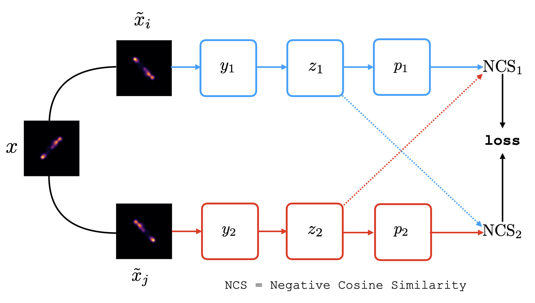
Figure 4: Schematic diagram of SimSiam— method. In the first blue branch, the prediction $p_{1}$ is matched with the representation $z_{2}$ using negative cosine similarity, indicated by ${\rm NCS}_{k=1,2}$. The dashed red arrow indicates that $z_{2}$ acts like a constant with zero gradient. Similarly in the second red branch, $p_{2}$ is matched with $z_{1}$ which is turned into a constant, as indicated by the dashed blue arrow.

and similar to BYOL, an augmented view of an image is predicted from another augmented view of the same image. In SimSiam, two different augmentations of the same image $\tilde{\bm{x}}_{i}$ and $\tilde{\bm{x}}_{j}$ are encoded to obtain two representations $y_{1}$ and $y_{2}$ respectively. The latter are in turn projected into a latent space, producing $z_{1}$ and $z_{2}$ respectively. The prediction $p_{1}$, which results from transforming $z_{1}$ via a projection head, is matched with the latent space representation $z_{2}$ of the second branch, by minimizing the negative cosine similarity [10]

$$\mathcal{D}(p_{1},z_{2})=-\frac{p_{1}}{||p_{1}||_{2}}\cdot\frac{z_{2}^{\rm stopgrad}}{||z_{2}^{\rm stopgrad}||_{2}},$$ (3.7)

where $z_{2}^{\rm stopgrad}$ denotes stop-gradient operation on $z_{2}$, which is the key aspect of the method. The prediction $p_{2}$ from the second branch is similarly matched with $z_{1}$ on which stop-gradient is acting as well and the total loss is given by [10]

$$\mathcal{L}=\frac{1}{2}(\mathcal{D}(p_{1},z_{2})+\mathcal{D}(p_{2},z_{1})).$$ (3.8)

We select Resnet-34 as the encoder in our implementation, and use LARS optimizer with learning rate 0.0005. We train the model for 1000 epochs, and choose a batch size 1024. Both the projector and predictor are one hidden layer MLP that converts their input into an array of length 128. We also use the same stochastic transformations chosen in the case of both SimCLR and BYOL. It is worth noting that we use lightly ssl [25] framework and follow the examples in their documentation to build the architecture of all the SSL based models in this work.

4 Results

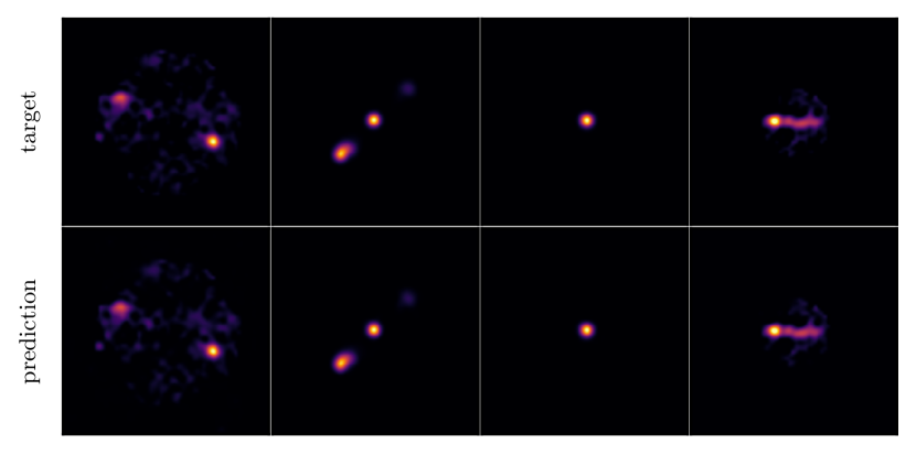
Figure 5: Reconstructing some examples of images from the test set from RGZ DR1 dataset. Top row denotes the images from the test set and the bottom row shows the corresponding images (i.e. output image of the decoder when feeding an input image) that are recovered by the decoder.

4.1 Reconstruction

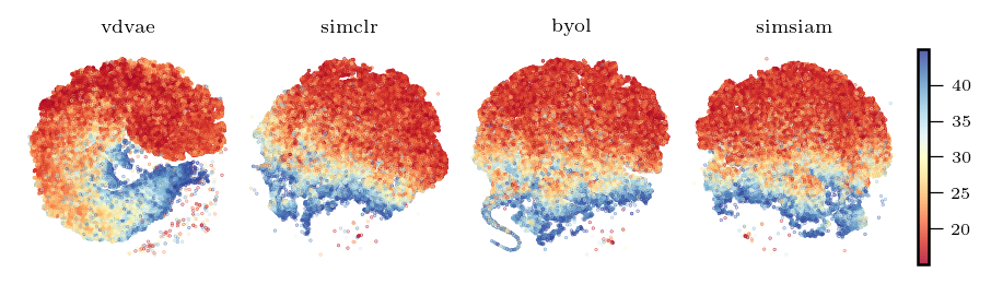
Figure 6: Latent space representations of galaxies from the training set learned by different methods, VDVAE—, SimCLR—, BYOL—, and SimSiam—. For visualisation, TSNE method is used. The color coding indicates the angular scale of the galaxy in arcseconds .

The top and bottom rows in Figure 5 show some examples of input images from the unlabeled test set of RGZ DR1 dataset and their corresponding reconstructions by the decoder respectively. Results suggest that the model is able to reconstruct the targets. VAE is known to suffer from blurry generated/reconstructed images, and the examples presented in Figure 5 have been cherry-picked to highlight the predictive power of the algorithm which can recover a diffuse jet of a target (e.g. last right panel of the bottom row). It can be noticed that visually the diffuse structures surrounding the hot spots in the first left panel top row are captured (see first left panel of the bottom row). Overall, all the fine details of the inputs are reconstructed reasonably well.

4.2 Latent codes

4.2.1 Visualization of the learned representations

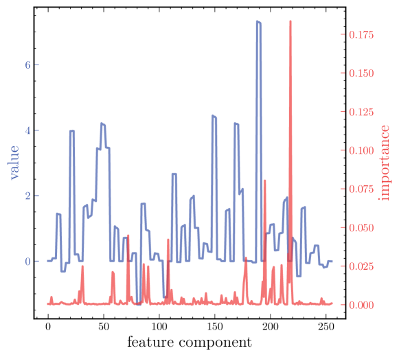
Figure 7: The blue and red lines denote the value and feature importance score as a function of feature component respectively. The representations are those learned by VDVAE—.

The entire training dataset is fed to each encoder in order to extract the representations which consist of vector of length 256 for the case of VDVAE and 512 for the SSL methods since they all use similar backbone, i.e. Resnet-34. For visualization, dimensionality reduction method is used to further project the encoded features into two dimensional subspace. We consider t-distributed stochastic neighbor embedding (TSNE) [26] in our analyses to demonstrate the ability of each representation learning model to compress the galaxy images. The first, second, third and fourth panels in Figure 6 show the results obtained from VDVAE, SimCLR, BYOL, and SimSiam respectively. Each data point in each panel in Figure 6 denotes the compression of each input image. The color coding indicates the projected angular size of the galaxies. Figure 6 shows that in general each method has learned good representations, as evidenced by the clustering of galaxies with similar angular scales in the 2D subspace. This already points to the fact that the performance of our generative model is on par with that of the selected SSL based methods. To analyze the features extracted by the generative model, we compute their importance. Provided that the RGZ DR1 dataset is unlabeled, but only the angular scales are given, we compute the feature importance using random forest regressor by building a mapping between the latent codes and angular scales. What we address here is whether the value of a component correlates with its importance in a specific setup, which is regression in our case, given the dataset. As the number of instances in the training set ($\sim$ 100,000) is relatively large for the algorithm, we train a random forest regressor with an inital number of estimators on the latent codes in batch of 1000. The number of estimators is increased by one when training with the next new batch. The results are presented in Figure 7. The solid blue line is the average value of each component of all the examples, whereas the solid red one denotes the importance (which is a score) of each component as outputted by the algorithm after training. Figure 7 shows that relatively few components carry information that is useful for inferring the angular scale of a galaxy image. In fact, by using Principal Components Analysis (PCA), we find that only two and four components encode $95\%$ and $98\%$ of the variance respectively. Figure 7 clearly shows that higher value of a feature component does not correlate with its importance for this regression task.

4.2.2 Using encoded features to classify galaxies

The trained encoders are used to extract the features of the galaxy images from both MBC and FR-DEEP NVSS, two labeled datasets that haven’t been seen by the models during training. Leveraging the latent codes, FRI and FRII galaxies in both datasets are classified by using a variety of non-neural network algorithms – $k$-nearest neighbors (knn), random forest (rf), support vector machine (svm), logistic regression (lr), gradient boosting (gb) and extra trees (ext). We use scikit-learn [27] to implement the classifiers whose hyperparameters are presented in Table 1

method	hyperparameters
knn	number of neighbours: 20
rf	number of base estimators: 260
svc	kernel: rbf; $\gamma$: 0.2; C: 100
lr	maximum iteration: 1000
grad	number of base estimators: 250
ext	number of base estimators: 400

Table 1: For each method, the presented hyperparameters are the ones that are different from their default values in scikit-learn—.

The metrics which are used to assess the classification performance of each method considered in this work are

• accuracy which is a percentage of the number of true prediction in the test set,

• roc-auc, also known as the degree of separability. In other words the ability of a classifier to differentiate between the classes.

• recall (or sensitivity), describing how well the algorithm minimizes the false negative,

• specificity which is a complement of recall and says how well the negative samples are predicted.

It is noted that when computing the metrics, FRII galaxies are the positive classes and FRI the negative ones. However, since the goal is to be able to differentiate between FRI and FRII, we aim at maximizing both recall and specificity which is equivalent to recall in case where FRI is considered as positive class. For this downstream task, the representations of a training set of a dataset (e.g. MBC), which are obtained from a given feature extractor (e.g. VDVAE) are used to train various classifiers which are then tested on the representations of a test set of the same dataset. We adopt the same procedure for testing all feature extractors on all labeled datasets. The results are shown in Table 2.
On MBC dataset, results suggest that overall the representations learned by VDVAE, compared to those by SSL methods, carry a bit more information such that ext classifier generalizes better, achieving accuracy of $82\%$ and roc-auc of 0.90. Moreover, both FRI and FRII are equally well classified, as evidenced by specificity and recall both equal to 0.82. The second, third, and fourth best classifiers, namely by rf, grad and knn respectively, on VDVAE derived representations outperform all the best classifiers (performance written in bold in Table 2) resulting from training on the SSL extracted representations. This further demonstrates the better quality of the latent codes (i.e. obtained from VDVAE). [14] and [28], both resorting to BYOL to learn the galaxy image representations from RGZ DR1, showed that by setting a threshold cut on the angular extent of the galaxies in RGZ DR1 (essentially removing the point source looking images from the training set) their knn achieved better accuracy $85.25\%$ as opposed to the case which includes all instances in RGZ DR1 when training their BYOL. We find that the performance of our knn on classifying the representations of MBC dataset, obtained from VDVAE, is similar to that of knn in [14] where a threshold cut of about 16 arcsec was adopted. And the ability of our ext method ($82\%$ accuracy) to classify MBC galaxies is on par with that of knn ($85.25\%$ accuracy) in [14] where 29 arcsec threshold was adopted.
On FR-DEEP NVSS dataset, it appears that the top classifiers in all setups perform equally well, with a slight advantage of lr method classifying the representations obtained from SimCLR. Interestingly, a simple logistic regression generalizes well on the SSL extracted representations overall, indicating a linear mapping between the targets and the learned features. [19] used deep CNN architecture whose weights had been previously trained on a different galaxy dataset for classification [29], an approach known as transfer learning which can be exploited when the number of training examples of a new task is relatively small. Their deep network achieved an accuracy of $73\%$, and roc-auc of 0.81, specificity $\sim 71\%$ and recall $\sim 88\%$ on FR-DEEP NVSS data. In comparison, all our top classifiers in all setups exhibit similar performance if not better. This demonstrates how relevant and powerful the compressed information is.

Algorithm	MBC				FR-DEEP NVSS
	acc	roc	spec	rec	acc	roc	spec	rec
VDVAE
knn	0.76	0.86	0.73	0.78	0.74	0.83	0.55	0.89
rf	0.80	0.89	0.80	0.80	0.80	0.83	0.73	0.86
svc	0.75	0.88	0.69	0.80	0.72	0.84	0.55	0.86
lr	0.73	0.82	0.63	0.82	0.72	0.85	0.50	0.89
grad	0.80	0.89	0.76	0.84	0.76	0.86	0.64	0.86
ext	0.82	0.90	0.82	0.82	0.80	0.87	0.73	0.86
SimCLR
knn	0.63	0.72	0.57	0.69	0.72	0.78	0.45	0.93
rf	0.67	0.76	0.55	0.78	0.74	0.82	0.50	0.93
svc	0.72	0.82	0.71	0.73	0.76	0.83	0.50	0.96
lr	0.71	0.73	0.63	0.78	0.86	0.84	0.77	0.93
grad	0.64	0.73	0.69	0.60	0.78	0.82	0.64	0.89
ext	0.67	0.75	0.55	0.78	0.76	0.82	0.55	0.93
BYOL
knn	0.63	0.72	0.67	0.60	0.72	0.78	0.41	0.96
rf	0.70	0.77	0.61	0.78	0.72	0.84	0.50	0.89
svc	0.73	0.77	0.73	0.73	0.84	0.88	0.68	0.96
lr	0.70	0.68	0.61	0.78	0.80	0.84	0.64	0.93
grad	0.64	0.68	0.59	0.69	0.76	0.81	0.55	0.93
ext	0.69	0.77	0.57	0.80	0.74	0.83	0.55	0.89
SimSiam
knn	0.59	0.70	0.61	0.56	0.74	0.81	0.45	0.96
rf	0.66	0.81	0.57	0.75	0.76	0.84	0.55	0.93
svc	0.67	0.77	0.61	0.73	0.74	0.86	0.45	0.96
lr	0.66	0.73	0.69	0.64	0.82	0.83	0.73	0.89
grad	0.71	0.76	0.71	0.71	0.80	0.85	0.64	0.93
ext	0.73	0.80	0.61	0.84	0.74	0.83	0.50	0.93

Table 2: Accuracy (acc), roc-auc (roc), specificity (spec) and recall (rec) values obtained from MiraBest Confident and FR-DEEP NVSS test sets for different classifiers; k-nearest neighbors (knn—), random forest (rf—), support vector machine (svc—), logistic regression (lr—), gradient boosting (grad—), extra trees (ext—). The bold font highlights the best performance on representations learned by a method.

4.3 Similarity search

Another downstream task that exploits the latent codes is similarity search, which consists of finding images within a dataset that are semantically similar to a query image, using the vector representations. If $\bm{\theta}^{\rm query}$ is the representation of the query and $\bm{\theta}^{j}$ that of any example from the dataset within which the search is conducted, the cosine similarity is given by

$$S(\bm{\theta}^{\rm query},\bm{\theta}^{j})=\frac{\bm{\theta}^{\rm query}\cdot\bm{\theta}^{j}}{||\bm{\theta}^{\rm query}||\>||\bm{\theta}^{j}||}.$$ (4.1)

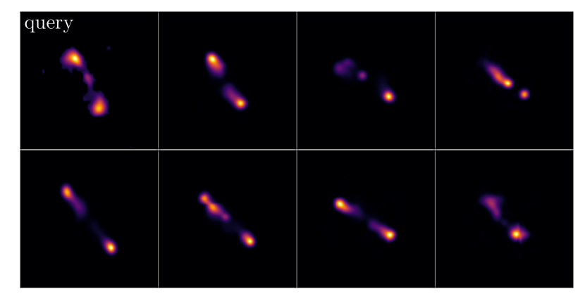
Figure 8: Similarity search exploiting the learned representations of galaxies. The top left image is the query from the test set in MBC and all the remaining images are obtained from searching in the RGZ DR1.

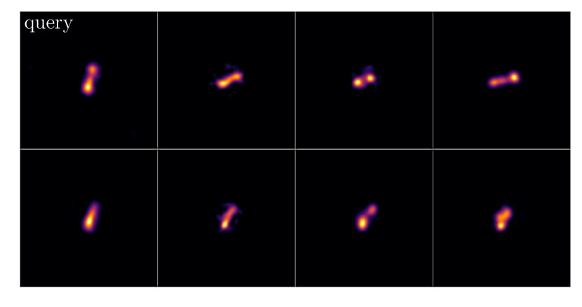
Figure 9: Similarity search where as opposed to Figure 8, the query image has a relatively small extension. The top left image is the query from the test set in MBC and all the remaining images are obtained from searching in the RGZ DR1.

The higher the score $S$ the more similar to the query an image from the dataset is. The query drawn from MBC dataset is used to search for galaxies which are semantically similar to it in RGZ DR1. Overall the galaxy images retrieved from the latter exhibit bright hotspots on both lobes and diffuse jets (Figure 8), which are features shared with the query shown in left panel on the top row of Figure 8. Interestingly, all galaxies in Figure 8 appear to show roughly the same inclination. The image query presented in Figure 8 has larger angular extensions, so for a further test, we carry out another search for galaxies with relatively small angular extension, but bigger than a point source so that some features are visible. Similar to the previous case, the query is selected from MBC and search is conducted in RGZ DR1. Figure 9 shows that the selected galaxies based on the query (top left panel in Figure 9) are semantically similar to the latter. They all roughly show diffuse emission between two bright lobes, and again are inclined in the same direction.

4.4 Generating new images

By sampling data points from the latent space and passing them through the decoder, new images are generated. We present in Figure 10 some examples of cherry-picked images that are produced by our model.

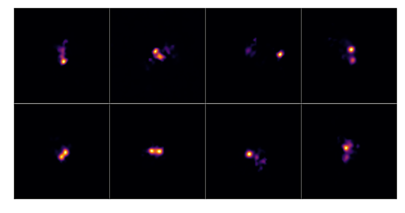
Figure 10: Examples of images that are generated by the trained decoder from sampling in the latent space.

Overall, the model is able to capture the salient features of the RGZ DR1 data, such as the hotspots and diffuse structures. It can be noticed that the projected angular scales of the generated images are relatively small, similar to those of the images in Figure 9 overall. It can be argued that this is due to the fact that the training dataset is strongly biased toward images with small angular size, as $\sim 70\%$ of the galaxies has less or equal than $35^{{}^{\prime\prime}}$ extension. It should be reiterated that the main objective is toward more compressing the data rather than the ability to generate new images (e.g. for data augmentation). But one possible solution, in order to reduce the effect of this bias in the generated images, is to train the generative model with a well balanced training set which contains roughly equal number of images with small and large angular scales. To further improve the quality of the generated images, the model can be conditioned on the angular extensions. We defer this to future work.

5 Estimating log-likelihood

We have seen in Section 4 that the latent codes carry meaningful information that can be exploited for some downstream tasks. The model parameters are optimized by maximizing the $\mathbb{ELBO}$ which is a lower limit of the log-likelihood. As such, estimating the log-likelihood of an input (or an entire dataset), within the context of identifying an out-of-distribution sample, is required. One way to address that is to directly train a density estimator on the $64\times 64$ pixels images. However, provided the usefulness of the latent representations with smaller dimensions compared with the images, they can also be used to train a density estimator so as to estimate the log-likelihood. In this section, we opt for the latter approach and train a Masked Autoregressive Flow (MAF) [30] – a state of the art density estimator – on the representations. We consider denmaf library [31] in our analyses, and first give a brief overview of normalizing flow and the MAF method before presenting the results.

5.1 Masked Autoregressive Flow (MAF)

Normalizing flow [32] is a type of generative model which consists of building an invertible differentiable mapping $f$: $\textbf{u}\rightarrow\textbf{x}$ between a data distribution $\textbf{x}\sim p(\textbf{x})$ and a base density $\textbf{u}\sim\pi_{u}(\textbf{u})$ (also known as prior) which is generally Gaussian. Using the change of variable formula, we have that [30]

$$p(\textbf{x})=\pi_{u}(f^{-1}(\textbf{x}))\left|{\rm det}\left(\frac{\partial f^{-1}}{\partial\textbf{x}}\right)\right|.$$ (5.1)

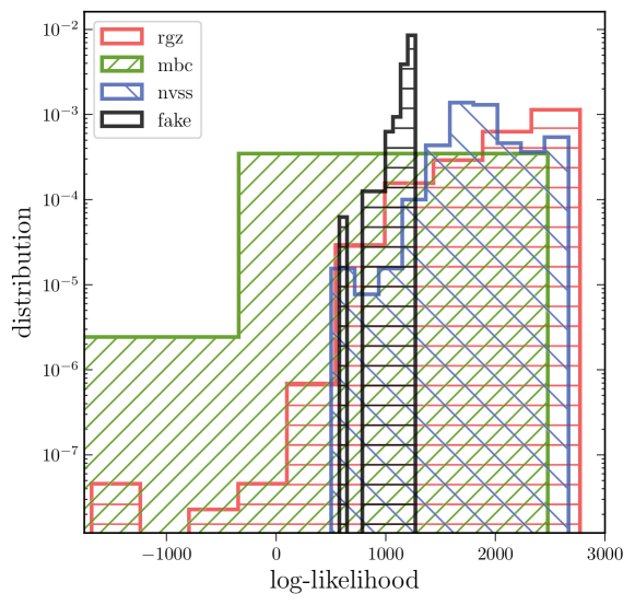
Figure 11: Histograms of log-likelihood of all samples in each dataset, RGZ DR1 (red), MBC (green) and FR-DEEP NVSS (blue). The log-likelihood distribution of new images generated by VDVAE— is shown in solid black line.

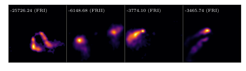
Figure 12: Out-of-distribution examples from MBC dataset based on the value of their loglikelihood which is the number presented on top of each image. The class of each galaxy from the MBC data is provided within round brackets.

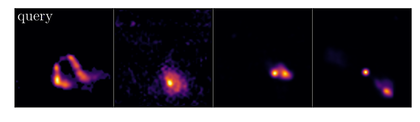
Figure 13: Search for images that are semantically similar to the an out-of-distribution sample (from MBC) in the RGZ DR1 data.

This formulation allows the density estimation of the data after training. To generate a new data point $\textbf{x}_{\rm new}$, the method samples a point u from the Gaussian prior and uses the mapping $f$. The density $p(\textbf{x})$ can be expressed as a product of conditionals $p(\textbf{x})=\prod_{i}p(x_{i}|\textbf{x}_{1:i-1})$, parameterized as Gaussians, such that the $i$th conditional is given by [30]

$$p(x_{i}|\textbf{x}_{1:i-1})=\mathcal{N}(x_{i}|u_{i},({\rm exp}\>\alpha_{i})^{2}),$$ (5.2)

where $u_{i}$ and $\alpha_{i}$ are computed using scalar functions, $u_{i}=f_{u_{i}}(\textbf{x}_{1:i-1})$ and $\alpha_{i}=f_{\alpha_{i}}(\textbf{x}_{1:i-1})$. The scalar functions ($f_{u_{i}},f_{\alpha_{i}}$) are constructed using Masked Autoencoder for Distribution Estimation (MADE) [33] which consists of dense layers. The autoregressive property is fulfilled by using appropriate masking, and making a conditional at $i$th MADE layer dependent on the previous one $i$-1th. In other words, MAF architecture is built by chaining up several MADE layers. There are several flow based models depending on how the invertible function is constructed, such as Real NVP [34], but in our study, we train MAF on the latent codes.

5.2 Log-likelihood of the data

We consider a MAF which comprises 48 MADE blocks, each block composed of 2 fully connected layers of 512 hidden neurons. We choose Adam optimizer with learning rate of 0.0005 and train the MAF model for 600 epochs on the latent codes of RGZ DR1 data. After training, we compute the log-likelihood of the representations of RGZ DR1, MBC and FR-DEEP NVSS and those of the new images generated by the decoder. Figure 11 shows the the log-likelihood histogram of each example in each dataset. The red, green, blue and black denote the log-likelihood distributions of RGZ DR1, MBC, FR-DEEP NVSS and fake images respectively. The fact that the support of the FR-DEEP NVSS log-likelihood distribution is a subset of the RGZ DR1 base distribution indicates that FR-DEEP NVSS instances are not out-of-distribution (OOD) with respect to RGZ DR1 dataset. In other words, the results suggest that the examples in both datasets are drawn from the same underlying distribution. However, it appears that some instances from the MBC data are considered OOD with respect to RGZ DR1, as demonstrated by some log-likelihood scores that are outside the support of the RGZ DR1 log-likelihood distribution. We present in Figure 12 instances that are associated with the lowest log-likelihood scores which, along with the class (withing round brackets), are provided on the top left corner of each panel. For example, the image shown on the first panel from the left, which has the lowest log-likelihood, appears to be a bent-tail galaxy whose jets are bent. The second panel, labeled as FRII, shows two bright lobes which do not appear to be from the same central galaxy based on the diffuse structure surrounding each of them. The third and fourth panels present a core with one-sided jet and a bright spot seemingly disconnected from a nearby faint object respectively. Provided that the learned representations can be utilized to retrieve similar images in a dataset, we search for images in RGZ DR1 that are semantically similar to the outlier corresponding to the lowest log-likelihood (top left panel in Figure 12). Search results are shown in Figure 13. On the one hand it is clear that none of the retrieved images are semantically similar to the query, demonstrating the efficiency of the density estimator to assign low log-likelihood to images with features that haven’t been seen during its training. On the other hand, interestingly, it can be noticed that, like the query, each galaxy image in Figure 13 is located on the bottom right corner of the panel. This shows that, although the patterns are not similar, the feature components of the latent codes are such that the group of pixels that carries most of the information is roughly located at the same corner in each panel of Figure 13. This test further demonstrates the meaningfulness of the learned representations. Lastly, Figure 11 also implies that the decoder is able to mimic RGZ DR1 data, as evidenced by the log-likelihood of each generated image that is well within the log-likelihood value range of the RGZ DR1 dataset.

6 Conclusion

We have shown in this work that it is possible to learn meaningful latent codes of radio galaxy images that can be leveraged for some downstream tasks. We have trained on an unlabeled dataset a variant of Variational AutoEncoder (VAE), whose both approximate posterior and prior are more expressive (compared to a vanilla VAE) by resorting to a hierarchical structure composed of many stochastic layers of latent variables. We have assessed the overall performance of our VAE model by looking at its ability to reconstruct the inputs, and analyzing how meaningful the representations it has learned during training are. In our investigation, we have also trained various SSL based methods, SimCLR, BYOL, SimSiam, and compared their performance in terms of classifying galaxies from labeled datasets with that of our model. The features extracted by each model are visualized in a two dimensional subspace by using t-SNE, a dimensionality reduction method. To investigate if the learned representations from different models carry meaningful information, six different classifiers – $k$-nearest neighbors (knn), random forest (rf), support vector machine (svc), logistic regression (lr), gradient boosting (grad), and extra trees (ext) – are trained on them in order to identify FRI/FRII galaxies from two different datasets. Similarity search, which is another downstream task employing the compressed data, has also been conducted. Although the capacity of the VDVAE model to generate new samples is not our primary objective in this work, we have checked how good it emulates the training data. Furthermore, we have estimated the log-likelihood of data by training a Masked Autoregressive Flow (MAF), a state of the art density estimator, on the latent codes. This is especially useful in the context of finding anomaly/novelty in a dataset. We summarize our findings as follows:

• Results suggest that our model is able to recover the inputs, capturing features like jet and diffuse structure, which indicates that the reconstructed images don’t seem to suffer from blurriness, a known issue with VAE models in general.

• The galaxy representations obtained from each model are well clustered with respect to angular size, implying that each method has properly learned to encode the high dimensional data.

• In a setup, the representations of galaxies from a labeled dataset, either MBC or FR-DEEP NVSS, are retrieved by a feature extractor (VDVAE, SimCLR, BYOL or SimSiam) and used to train several non-neural network classifiers. In general, for MBC dataset, the information carried by the features extracted by the generative model has slightly better quality compared to those by the SSL based models. The four best classifiers trained on the VDVAE latent codes – all achieving accuracy $\geq 76\%$, roc-auc $\geq 0.86$, specificity $\geq 0.73$ and recall $\geq 0.78$ – outperform all the best classifiers of other setups in this work. The results on classifying galaxies in MBC dataset using learned representations also show that the performance of our generative model is comparable to that of the model in [14]. The top classifiers in all setups perform equally well on the FR-DEEP NVSS dataset. Interestingly, the performance of simple classifiers in our analyses is on par, if not better, with that of a CNN based model used in [19]. This shows how meaningful the learned representation is.

• The learned representations can be used for similarity search, as evidenced by the retrieved images that are semantically similar to the query image. We carry out searches for galaxies with large and small angular sizes. The results in both cases are consistent in the sense that all the images found exhibit similar patterns. In addition, the inclination of the galaxy in the query image is roughly found in all galaxies returned by the search. The importance of this application was highlighted in [11], where the encoded features were leveraged to search for similar images in a large dataset.

• We find that the decoder is capable of generating new images that are comparable with the training data overall. Neverthless, the generated images tend to be of smaller angular size, which can attributed to the bias in the dataset. The possibility that the decoder still lacks power, and hence requires more fine-tuning, can not be ruled out. However, a sufficiently powerful decoder is prone to a posterior collapse [35, 36] where the latent codes is no longer useful as they haven’t been learned by the model. Provided that the main objective in this study is to learn the latent codes, increasing the power of the decoder in order to optimize the ability of the model to generate fake images needs to be approached carefully.

• The galaxies in FR-DEEP NVSS appear to have been drawn from the same distribution as those in RGZ DR1 dataset. This is evidenced by the log-likelihood values of the former which lie within the range of those from the latter. However, some galaxies withing MBC dataset are associated with log-likelihood scores outside RGZ DR1 base distribution, and therefore are considered OOD (solely based on the likelihood as a metric). As a way to further validate both the usefulness of the latent codes and the density estimation by the MAF model, we search for images in RGZ DR1 that are semantically similar to the OOD instance (from MBC) associated with the lowest log-likelihood. We find that the search fails to return similar galaxies, corroborating the fact that the query image is indeed an OOD with respect to RGZ DR1 dataset. It is also found that the new images generated by the decoder are in-distribution with respect to RGZ DR1, as the estimated log-likelihood of each new instance is well within the log-likelihood distribution of RGZ DR1. It is worth noting that although both the VDVAE encoder and decoder are trained simultaneously on the RGZ DR1 data, the new images which are obtained by sampling from latent space and reconstruction via the decoder have never been seen by the encoder which extracts the latent codes. This shows that the decoder is able to emulate the RGZ DR1 data.

The generative model in this work has shown promising performance. For future investigation one question that can be addressed is the impact of the input dimensions on the results, for instance by considering $128\times 128$ pixels resolution of the images used for training. This is one way to assess the robustness of the method.

References

- [1] A. Dey, D. J. Schlegel, D. Lang, R. Blum, K. Burleigh, X. Fan, J. R. Findlay, D. Finkbeiner, D. Herrera, S. Juneau, et al., Overview of the desi legacy imaging surveys, The Astronomical Journal 157 (2019), no. 5 168.
- [2] J. E. Gunn, M. Carr, C. Rockosi, M. Sekiguchi, K. Berry, B. Elms, E. De Haas, Ž. Ivezić, G. Knapp, R. Lupton, et al., The sloan digital sky survey photometric camera, The Astronomical Journal 116 (1998), no. 6 3040.
- [3] J. E. Gunn, W. A. Siegmund, E. J. Mannery, R. E. Owen, C. L. Hull, R. F. Leger, L. N. Carey, G. R. Knapp, D. G. York, W. N. Boroski, et al., The 2.5 m telescope of the sloan digital sky survey, The Astronomical Journal 131 (2006), no. 4 2332.
- [4] J. K. Banfield, O. Wong, K. W. Willett, R. P. Norris, L. Rudnick, S. S. Shabala, B. D. Simmons, C. Snyder, A. Garon, N. Seymour, et al., Radio galaxy zoo: host galaxies and radio morphologies derived from visual inspection, Monthly Notices of the Royal Astronomical Society 453 (2015), no. 3 2326–2340.
- [5] P. E. Dewdney, P. J. Hall, R. T. Schilizzi, and T. J. L. Lazio, The square kilometre array, Proceedings of the IEEE 97 (2009), no. 8 1482–1496.
- [6] A. Weltman, P. Bull, S. Camera, K. Kelley, H. Padmanabhan, J. Pritchard, A. Raccanelli, S. Riemer-Sørensen, L. Shao, S. Andrianomena, et al., Fundamental physics with the square kilometre array, Publications of the Astronomical Society of Australia 37 (2020) e002.
- [7] T. Chen, S. Kornblith, M. Norouzi, and G. Hinton, A simple framework for contrastive learning of visual representations, in International conference on machine learning, pp. 1597–1607, PMLR, 2020.
- [8] J.-B. Grill, F. Strub, F. Altché, C. Tallec, P. Richemond, E. Buchatskaya, C. Doersch, B. Avila Pires, Z. Guo, M. Gheshlaghi Azar, et al., Bootstrap your own latent-a new approach to self-supervised learning, Advances in neural information processing systems 33 (2020) 21271–21284.
- [9] K. He, H. Fan, Y. Wu, S. Xie, and R. Girshick, Momentum contrast for unsupervised visual representation learning, in Proceedings of the IEEE/CVF conference on computer vision and pattern recognition, pp. 9729–9738, 2020.
- [10] X. Chen and K. He, Exploring simple siamese representation learning, in Proceedings of the IEEE/CVF conference on computer vision and pattern recognition, pp. 15750–15758, 2021.
- [11] G. Stein, P. Harrington, J. Blaum, T. Medan, and Z. Lukic, Self-supervised similarity search for large scientific datasets, arxiv:2110.13151.
- [12] M. A. Hayat, G. Stein, P. Harrington, Z. Lukić, and M. Mustafa, Self-supervised representation learning for astronomical images, The Astrophysical Journal Letters 911 (2021), no. 2 L33.
- [13] T. Chen, S. Kornblith, K. Swersky, M. Norouzi, and G. E. Hinton, Big self-supervised models are strong semi-supervised learners, Advances in neural information processing systems 33 (2020) 22243–22255.
- [14] I. V. Slijepcevic, A. M. Scaife, M. Walmsley, and M. Bowles, Learning useful representations for radio astronomy” in the wild” with contrastive learning, arxiv:2207.08666.
- [15] D. J. Bastien, A. M. Scaife, H. Tang, M. Bowles, and F. Porter, Structured variational inference for simulating populations of radio galaxies, Monthly Notices of the Royal Astronomical Society 503 (2021), no. 3 3351–3370.
- [16] H. Miraghaei and P. Best, The nuclear properties and extended morphologies of powerful radio galaxies: the roles of host galaxy and environment, Monthly Notices of the Royal Astronomical Society 466 (2017), no. 4 4346–4363.
- [17] F. Porter, Mirabest batched dataset, .
- [18] F. A. Porter and A. M. Scaife, Mirabest: a data set of morphologically classified radio galaxies for machine learning, RAS Techniques and Instruments 2 (2023), no. 1 293–306.
- [19] H. Tang, A. M. Scaife, and J. Leahy, Transfer learning for radio galaxy classification, Monthly Notices of the Royal Astronomical Society 488 (2019), no. 3 3358–3375.
- [20] D. P. Kingma and M. Welling, Auto-encoding variational bayes, arxiv:1312.6114.
- [21] C. P. Burgess, I. Higgins, A. Pal, L. Matthey, N. Watters, G. Desjardins, and A. Lerchner, Understanding disentangling in -vae, arxiv:1804.03599.
- [22] R. Child, Very deep vaes generalize autoregressive models and can outperform them on images, arxiv:2011.10650.
- [23] A. v. d. Oord, Y. Li, and O. Vinyals, Representation learning with contrastive predictive coding, arXiv preprint arXiv:1807.03748 (2018).
- [24] K. He, X. Zhang, S. Ren, and J. Sun, Deep residual learning for image recognition, in Proceedings of the IEEE conference on computer vision and pattern recognition, pp. 770–778, 2016.
- [25] I. Susmelj, M. Heller, P. Wirth, J. Prescott, and M. E. et al., Lightly, GitHub. Note: https://github.com/lightly-ai/lightly (2020).
- [26] L. Van der Maaten and G. Hinton, Visualizing data using t-sne., Journal of machine learning research 9 (2008), no. 11.
- [27] F. Pedregosa, G. Varoquaux, A. Gramfort, V. Michel, B. Thirion, O. Grisel, M. Blondel, P. Prettenhofer, R. Weiss, V. Dubourg, et al., Scikit-learn: Machine learning in python, Journal of machine learning research 12 (2011), no. Oct 2825–2830.
- [28] I. V. Slijepcevic, A. M. Scaife, M. Walmsley, M. Bowles, O. Wong, S. S. Shabala, and S. V. White, Radio galaxy zoo: Building a multi-purpose foundation model for radio astronomy with self-supervised learning, arXiv preprint arXiv:2305.16127 (2023).
- [29] A. Aniyan and K. Thorat, Classifying radio galaxies with the convolutional neural network, The Astrophysical Journal Supplement Series 230 (2017), no. 2 20.
- [30] G. Papamakarios, T. Pavlakou, and I. Murray, Masked autoregressive flow for density estimation, Advances in neural information processing systems 30 (2017).
- [31] R. K. Lo, denmarf: a python package for density estimation using masked autoregressive flow, arxiv:2305.14379.
- [32] D. Rezende and S. Mohamed, Variational inference with normalizing flows, in International conference on machine learning, pp. 1530–1538, PMLR, 2015.
- [33] M. Germain, K. Gregor, I. Murray, and H. Larochelle, Made: Masked autoencoder for distribution estimation, in International conference on machine learning, pp. 881–889, PMLR, 2015.
- [34] L. Dinh, J. Sohl-Dickstein, and S. Bengio, Density estimation using real nvp, arXiv preprint arXiv:1605.08803 (2016).
- [35] A. Alemi, B. Poole, I. Fischer, J. Dillon, R. A. Saurous, and K. Murphy, Fixing a broken elbo, in International conference on machine learning, pp. 159–168, PMLR, 2018.
- [36] X. Chen, D. P. Kingma, T. Salimans, Y. Duan, P. Dhariwal, J. Schulman, I. Sutskever, and P. Abbeel, Variational lossy autoencoder, arxiv:1611.02731.