Peak Estimation of Rational Systems using Convex Optimization

Abstract

This paper presents algorithms that upper-bound the peak value of a state function along trajectories of a continuous-time system with rational dynamics. The finite-dimensional but nonconvex peak estimation problem is cast as a convex infinite-dimensional linear program in occupation measures. This infinite-dimensional program is then truncated into finite-dimensions using the moment-Sum-of-Squares (SOS) hierarchy of semidefinite programs. Prior work on treating rational dynamics using the moment-SOS approach involves clearing dynamics to common denominators or by adding lifting variables to handle reciprocal terms under new equality constraints. Our solution method uses a sum-of-rational method based on absolute continuity of measures. The Moment-SOS truncations of our program possess lower computational complexity and (empirically demonstrated) higher accuracy of upper bounds on example systems as compared to prior approaches.

I Introduction

Peak estimation is the practice of finding extreme values of a state function $p$ along trajectories $x(t)$ of a dynamical system that evolve starting from an initial set $X_{0}$. Instances of peak estimation (extremizing $p(x(t))$) include finding the maximum speed of an aircraft, height of a rocket, concentration of a chemical, and current along a transmission line. This work focuses on peak estimation in the case of rational continuous-time dynamics for a state $x\in\mathbb{R}^{n}$ where:

$$\dot{x}(t)=f(t,x),$$ (1)

where the rational dynamics $f$ can be represented as

$$f(t,x) =f_{0}(t,x)+\sum_{\ell=1}^{L}\frac{N_{\ell}(t,x)}{D_{\ell}(t,x)}.$$ (2)

The expression in (1) is a sum-of-rational dynamical system in terms of polynomials $N_{\ell}$ and $D_{\ell}$ (with $L$ finite). Applications of peak estimation for rational systems include systems include finding maximal concentrations in chemical reaction networks with Michaelis-Menten kinetics or yeast glycolysis, velocities in rigid body kinematics (manipulator equation with rational friction models), and occupancies in network queuing models [1, 2]. Refer to [1] for a detailed survey of applications of rational systems, as well as a formulation of algebraic analysis techniques to establish system properties such as parameter identifiability and controllability.

The rational-dynamics peak estimation task considered in this work (maximizing a state function $p$ along system trajectories evolving in a state space $X\in\mathbb{R}^{n}$ starting from $X_{0}\subseteq X$ with a time horizon of $[0,T]$) is described in Problem 1.

Problem 1

Find an initial condition $x_{0}$ and a stopping time $t^{*}$ to extremize:

$$P^{*}= \ \sup_{t^{*},x_{0}}\ p(x(t^{*}\mid x_{0}))$$ (3a)

subject to $$\dot{x}(t)=f(t,x(t))\qquad\textrm{from \eqref{eq:rational_dynamics}}$$ (3b)

$$t^{*}\in[0,T],\quad x_{0}\in X_{0}.$$ (3c)

The Ordinary Differential Equation (ODE) peak estimation problem in (3) is an instance of OCP Optimal Control Problem (OCP) with a free terminal time and zero stage (integral) cost. The finite-dimensional problem (3) is generically nonconvex in $(t^{*},x_{0})$, but can be lifted into a pair of primal-dual infinite-dimensional Linear Programs in occupation measures [3]. Computational solution methods for derived measure LPs include gridding-based discretization [4], random sampling [5], and the moment- Sum of Squares (SOS) hierarchy of Semidefinite Programs [6, 7, 8]. Peak estimation LPs have been developed for dynamical systems such as robustly uncertain systems [9, 10], stochastic systems (mean and value-at-risk) [4, 11], time-delay systems [12], and hybrid systems [13]. Other problem domains in which infinite-dimensional LPs have been used in the analysis and control of dynamical systems include reachable set estimation and backwards-reachable-set maximizing control [14, 15, 16, 17, 18], maximum positively invariant set estimation [19], maximum controlled invariant sets [20], global attractors [21], and long-time averages [22].

All of the previously mentioned applications of LP in dynamical systems analysis and control (in the context of continuous state spaces) use a Lipschitz assumption in dynamics in order to prove that there is no relaxation gap between the infinite-dimensional LP and the original finite-dimensional nonconvex program. The rational dynamics in (1) may fail to be globally Lipschitz (within the domain of $[0,T]\times X$), and therefore falls into the theory of nonsmooth dynamical systems [23, 24, 25]. This work utilizes a sum-of-rational representation from [26] in order to cast (3) as an LP in measures, and uses the theory of nonsmooth Liouville equations from [23] to prove equivalence of optima under compactness, trajectory-uniqueness, and positivity assumptions. Prior work in SOS-based analysis of rational functions includes clearing to common denominators [27] (under positivity), and adding new variables to represent the graph of rational functions as equality constraints [28, 29].

The main contributions of this work are:

• A measure LP formulation for peak estimation of rational dynamical systems based on the theory of [26] (for sum-of-rational static optimization).

• A proof that there is no relaxation gap between the finite-dimensional nonconvex problem (3) and the objectives of infinite-dimensional LPs

• A proof strong duality between the rational-system peak estimation infinite-dimensional LPs.

• Quantification of the computational complexity in terms of sizes of the Positive Semidefinite (PSD) matrices in SDPs.

• Experiments demonstrating the upper-bounding of the true peak on rational dynamical systems.

This paper has the following structure: Section II reviews preliminaries such as notation and occupation measures. Section III formulates a sum-of-rational-based measure LP for the peak estimation problem in (3). Section IV introduces and applies the moment-SOS hierarchy to obtain a nonincreasing sequence of upper-bounds to the true peak value $P^{*}$. Section V performs peak estimation on example rational dynamical systems. Section VI concludes the paper. Appendix A provides a proof of strong duality between the measure and function LPs. Appendix B documents SOS programs for pre-existing rational-peak-estimation methods [27, 28].

II Preliminaries

BSA

Basic Semialgebraic

LP

Linear Program

OCP

Optimal Control Problem

ODE

Ordinary Differential Equation

PSD

Positive Semidefinite

SDP

Semidefinite Program

SOS

Sum of Squares

WSOS

Weighted Sum of Squares

II-A Notation

The set of $n$-dimensional indices with sum less than or equal to a value $d$ is $\mathbb{N}^{n}_{\leq d}$ ($\alpha\in\mathbb{N}_{d}^{n}$ if $\alpha\in\mathbb{N}^{n}$ and $\sum_{i=1}^{n}\alpha_{i}\leq d$). The set of polynomials with indeterminate $x$ is $\mathbb{R}[x]$, and the subset of polynomials with degree at most $d$ is $\mathbb{R}[x]_{\leq d}$.

The set of continuous (continuous and nonnegative) functions over $S$ is $C(S)$ ($C_{+}(S)$). The set of signed (nonnegative) Borel measures over a set $S$ is $\mathcal{M}(S)$ ($\mathcal{M}_{+}(S)$). The measure of a set $A\subseteq S$ w.r.t. $\mu\in\mathcal{M}_{+}(S)$ is $\mu(A)$. The sets $C_{+}(S)$ and $\mathcal{M}_{+}(S)$ possess a bilinear pairing $\langle\cdot,\cdot\rangle$ that acts by Lebesgue integration: $g\in C_{+}(S),\mu\in\mathcal{M}_{+}(S):\langle g,\mu\rangle=\int_{S}g(s)d\mu(s)$. This bilinear pairing is an inner product between $C_{+}(S)$ and $\mathcal{M}_{+}(S)$ when $S$ is compact, and the pairing can be extended to integration between $C(S)$ (and sets of more general measurable functions) and $\mathcal{M}(S)$. Given two mesures $\mu_{1}\in\mathcal{M}_{+}(S_{1}),\mu_{2}\in\mathcal{M}_{+}(S_{2})$, the product measure $\mu_{1}\otimes\mu_{2}$ is the unique measure satisfying $\forall A_{1}\subseteq S_{1},\ A_{2}\subseteq S_{2}:\ (\mu_{1}\otimes\mu_{2})(A_{1}\times A_{2})=\mu_{1}(A_{1})\mu_{2}(A_{2})$. Given a set $A\subseteq S$, the $0/1$ indicator function $I_{A}$ takes on value $I_{A}(s)=1$ if $s\in A$ and $I_{A}(s)=0$ if $s\notin A$ (ensuring that $\langle I_{A}(S),\mu\rangle=\mu(A)$). The mass of a measure $\mu\in\mathcal{M}_{+}(S)$ is $\mu(S)=\langle 1,S\rangle$, and $\mu$ is a probability measure if this mass is 1. The Dirac delta supported at a point $s^{\prime}$ ($\delta_{s=s^{\prime}}$) is the unique probability measure such that $\forall g\in C(\mathcal{S}):\langle g,\delta_{s=s^{\prime}}\rangle=g(s^{\prime})$. The adjoint of a linear operator $\mathscr{L}$ is $\mathscr{L}^{\dagger}$.

II-B Occupation Measures

An occupation measure is a nonnegative Borel measure that contains all possible information about the behavior of (a set of) trajectories of a given dynamical system.

For a given initial condition $x_{0}\in X_{0}$, the occupation measure $\mu_{x(\cdot)}\in\mathcal{M}_{+}([0,T]\times X)$ of the trajectory $x(t\mid x_{0})$ (3b) up to a stopping time $t^{*}\in[0,T]$ satisfies $\forall A\in[0,T],\ B\in X$:

$$\mu_{x(\cdot)}(A\times B\mid t^{*})= \int_{[0,t^{*}]}I_{A\times B}\left((t,x(t\mid x_{0})\right)dt.$$ (4)

The $(t^{*},x_{0}^{*})$-occupation measure $\mu_{x(\cdot)}$ in (4) can also be understood in terms of its pairing with arbitrary continuous (measurable) functions:

$$\forall\omega\in C([0,T]\times X) \langle v,\mu_{x(\cdot)}\rangle =\textstyle\int_{0}^{t^{*}}\omega(t,x(t\mid x_{0}))dt.$$ (5)

Occupation measures $\mu_{x(\cdot)}$ in (4) may be defined over a distribution of initial conditions $\mu_{0}\in\mathcal{M}_{+}(X_{0})$ (with $x_{0}\sim\mu_{0}$):

$$\mu(A\times B\mid t^{*})= \int_{X_{0}}\int_{[0,t^{*}]}I_{A\times B}\left((t,x(t\mid x_{0})\right)dtd\mu_{0}(x_{0}).$$

The Lie derivative (instantaneous change) of a test function $v\in C^{1}([0,T]\times X)$ w.r.t. dynamics (1) is

$$\mathcal{L}_{f}v(t,x)=\partial_{t}v(t,x)+f(t,x)\cdot\nabla_{x}v(t,x).$$ (6)

Any trajectory of (3b) satisfies the conservation law,

$$v(t^{*},x(t\mid x_{0}))=v(0,x_{0})+\int_{0}^{t^{*}}\mathcal{L}_{f}v(t^{\prime},x(t^{\prime}\mid x_{0}))dt^{\prime}.$$ (7)

The conservation law in (7) is a Liouville equation, and can be written in terms of the initial measure $\mu_{0}=\delta_{x=x_{0}}\in\mathcal{M}_{+}(X_{0})$, terminal measure $\mu_{p}=\delta_{t=t^{*},x=x(t^{*}\mid x_{0})}\in\mathcal{M}_{+}([0,T]\times X)$, and occupation measure $\mu=\mu_{x(\cdot)}\in\mathcal{M}_{+}([0,T]\times X)$ for all $v$ as [23]

$$\langle v(t,x),\mu_{p}\rangle =\langle v(0,x),\mu_{0}\rangle+\langle\mathcal{L}_{f}v(t,x),\mu\rangle.$$ (8)

The $$\forall v \mathcal{L}_{f}^{\dagger} \mathcal{L}$$ imposition in equation (8) can be written equivalently in shorthand form (with as the adjoint linear operator of ) as

$$\mu_{p} =\delta_{0}\otimes\mu_{0}+\mathcal{L}_{f}^{\dagger}\mu.$$ (9)

Any triple $(\mu_{0},\mu_{p},\mu)$ that satisfies (9) is a relaxed occupation measure; the class of relaxed occupation measures may be larger than the set of superpositions (distributions) of occupation measures arising from trajectories.

III Rational Linear Program

This section will present convex infinite-dimensional LP to perform peak estimation of rational systems.

III-A Assumptions

We will begin with the following assumption:

• If a trajectory satisfies $x(t\mid x_{0})\not\in X$ for some $x_{0}\in X_{0}$, then $x(t^{\prime}\mid x_{0})\not\in X$ for all $t^{\prime}\geq t$.

Further assumptions will be added as needed.

Remark 2

Assumption A1 is a non-return assumption in the style of [30].

III-B Measure Program

Problem 3 introduces LP LP in measures to produce an upper-bound on Problem 1 [3, 4]:

Problem 3

Find an initial measure $\mu_{0}$, a relaxed occupation measure $\mu$, and a peak measure $\mu_{p}$ to supremize

$$p^{*}= \ \sup\quad\langle p,\mu_{p}\rangle$$ (10a)

subject to: $$\mu_{p}=\delta_{0}\otimes\mu_{0}+\mathcal{L}_{f}^{\dagger}\mu$$ (10b)

$$\langle 1,\mu_{0}\rangle=1$$ (10c)

$$\mu,\mu_{p}\in\mathcal{M}_{+}([0,T]\times X)$$ (10d)

$$\mu_{0}\in\mathcal{M}_{+}(X_{0}).$$ (10e)

Theorem 4

Under Assumption A1, Problem 3 will upper-bound 1 with $p^{*}\geq P^{*}$

Proof:

Let $(t^{*},x_{0}^{*})\in[0,T]\times X_{0}$ be a feasible point of (3), such that $\forall t\in[0,t^{*}]:\ x(t\mid x_{0}^{*})\in X$. One such feasible point is the tuple $(0,x^{*}_{0})$ for any $x^{*}_{0}\in X_{0}$. A feasible relaxed occupation measure $(\mu_{0},\mu_{p},\mu)$ may be constructed from the trajectory $x(t\mid x_{0}^{*})$: with an initial measure $\mu_{0}=\delta_{x=x_{0}^{*}},$ a peak measure $\mu_{p}=\delta_{t=t^{*},\ x=x(t\mid x_{0}^{*})},$ and an occupation measure of $\mu=\mu_{x(\cdot)}$. This relaxed occupation measure satisfies constraints (10b)-(10e) and has objective $\langle p,\mu_{p}\rangle=p(x(t^{*}\mid x_{0}^{*})).$ The upper-bound $p^{*}\geq P^{*}$ is proven because every $(t^{*},x_{0}^{*})$ has a measure representation. ∎

Equality of the objectives of Problem 1 and 3 will occur under a set of additional assumptions:

• The set $[0,T]\times X_{0}\times X$ is compact.

• The cost $p(x)$ is continuous.

• Trajectories of (3b) starting at $X_{0}$ in times $[0,T]$ are unique.

Theorem 5

Under assumptions A1-A4, the relation $p^{*}=P^{*}$ will hold.

Proof:

By Theorem 3.1 of [24], imposition of assumption A4 ensures that every relaxed occupation measure $(\mu_{0},\mu_{p},\mu)$ is supported on the graph of (a superposition of) trajectories of (3b). Compactness (A2) and (lower semi-) continuity (A3) are necessary to invoke arguments used by Theorem 2.1 of [3], using the non-smooth Theorem 3.1 of [24] rather than a Lipschitz assumption on dynamics. ∎

III-C Absolute Continuity Formulation

We will use the sum-of-rationals framework of [26] in order to express (10) in a form more amenable to numerical computation, using the moment-SOS hierarchy of SDPs. This sum-of-rationals framework uses the notion of absolute continuity of measures.

Definition 6

A measure $\nu\in\mathcal{M}_{+}(S)$ is absolutely continuous to $\mu\in\mathcal{M}_{+}(S)$ ($\nu\ll\mu$) if, for every $A\subseteq X$, $\langle I_{A},\mu\rangle=0$ implies that $\langle I_{A},\nu\rangle=0$.

Definition 7

For every pair of absolutely continuous measures $\nu\ll\mu$, there exists a nonnegative function $h(s)$ such that $\forall g\in C(S):\ \langle g(s),\nu(s)\rangle=\langle g(s)h(s),\mu(s)\rangle$. This function $h$ is also referred to as the density of $\nu$ w.r.t. $\mu$, or as the Radon-Nikodym derivative $\frac{d\nu}{d\mu}$.

Given a dynamics $(f_{0},{N_{\ell}}_{\ell=1}^{L},{D_{\ell}}_{\ell=1}^{L})$ in (1) and a relaxed occupation measure $(\mu_{0},\mu_{p},\mu)$ feasible for (10), we can define a set of per-rational measures $\{\nu_{\ell}\}_{\ell=1}^{L}$ (with $\forall\ell:\nu_{\ell}\in\mathcal{M}_{+}([0,T]\times X)$). These per-rational measures will be constructed to satisfy the following condition with respect to the rational denominators in (2)

$$\forall\omega\in C([0,T]\times X),\ell\in 1..L:$$

$$\qquad\langle\omega(t,x)D_{\ell}(t,x),\nu_{\ell}(t,x)\rangle=\langle\omega(t,x),\mu(t,x)\rangle.$$ (11)

This condition will be expressed in condensed notation as

$$\forall\ell:\ D_{\ell}^{\dagger}\nu_{\ell}=\mu.$$ (12)

Remark 8

Equation (11) is inspired by Equation (7) of [26] for sum-of-rational optimization.

We now impose the following assumption:

• Each function $D_{\ell}$ is strictly positive over $[0,T]\times X$.

Proposition 9

The measures $\nu_{\ell}$ have finite densities $\frac{d\nu_{\ell}}{d\mu}=1/D_{\ell}$ when A5 is in effect.

The Lie derivative in (10b) can be expanded using (11) as ($\forall v\in C^{1}([0,T]\times X)$ with assumption A5 in place)

$$\langle\mathcal{L}_{f}v,\mu\rangle =\left\langle\partial_{t}v+\textstyle\left(f_{0}+\sum_{\ell=1}^{L}(N_{\ell}/D_{\ell})\right)\cdot\nabla_{x}v,\mu\right\rangle$$ (13a)

$$\langle\mathcal{L}_{f_{0}}v+\textstyle\sum_{\ell=1}^{L}(N_{\ell}/D_{\ell})\cdot\nabla_{x}v,\mu\rangle$$ (13b)

$$=\langle\mathcal{L}_{f_{0}}v,\mu\rangle+\textstyle\sum_{\ell=1}^{L}\langle(N_{\ell}/D_{\ell})\cdot\nabla_{x}v(t,x),\mu\rangle$$ (13c)

$$=\langle\mathcal{L}_{f_{0}}v,\mu\rangle+\textstyle\sum_{\ell=1}^{L}\langle N_{\ell}\cdot\nabla_{x}v,\nu_{\ell}\rangle.$$ (13d)

Problem 10 uses the sum-of-rational framework to pose a measure peak estimation LP:

Problem 10

Find an initial measure $\mu_{0}$, a relaxed occupation measure $\mu$, a peak measure $\mu_{p}$, and a set of per-rational measures $\{\nu_{\ell}\}_{\ell=1}^{L}$ to supremize

$$p^{*}_{r}= \ \sup_{\mu_{0},\mu,\ \mu_{p},\{\nu_{\ell}\}}\quad\langle p,\mu_{p}\rangle$$ (14a)

s.t. $$\mu_{p}=\delta_{0}\otimes\mu_{0}+\mathcal{L}_{f_{0}}^{\dagger}\mu+\textstyle\sum_{\ell=1}^{\ell}(N_{\ell}\cdot\nabla_{x})^{\dagger}\nu_{\ell}$$ (14b)

$$\forall\ell:\ \ D_{\ell}^{\dagger}\nu_{\ell}=\mu$$ (14c)

$$\langle 1,\mu_{0}\rangle=1$$ (14d)

$$\mu,\mu_{p},\{\nu_{\ell}\}\in\mathcal{M}_{+}([0,T]\times X)$$ (14e)

$$\mu_{0}\in\mathcal{M}_{+}(X_{0}).$$ (14f)

Corollary 11

Under A1-A5, the objective values of Problem 1 and 10 will be equal with $P^{*}=p^{*}_{r}$.

Proof:

Theorem 5 ensures that $P^{*}=p^{*}$ under A1-A4. The finite nature of the densities $1/D_{\ell}$ from Proposition 9 (proved by Theorem 2.1 of [26]) ensures that the absolute-continuity-based construction process in (11) will result each $\nu_{\ell}$ having identical support to $\mu$. As a result, $(\mu_{0},\mu_{p},\mu)$ from (14b) will form a relaxed occupation measure, thus ensuring no relaxation gap by Theorem 3.1 of [24] (used in Theorem 5). ∎

Remark 12

If A5 is not imposed, then it is possible for the measure $\nu_{\ell}$ from (11) to be unconstrained (with $D_{\ell}=0$ at some $(t,x)$). It therefore cannot be presumed that the supports of $\nu_{\ell}$ and $\mu$ are identical. These degrees of freedom in $\nu_{\ell}$ could allow for the strict (and possibly unbounded) upper-bound $p^{*}_{r}>p^{*}$.

III-D Function Program

The dual LP for 10 is contained in Problem 13:

Problem 13

Find a $C^{1}$ auxiliary function $v$, a scalar $\gamma$, and per-rational continuous functions $\{q_{\ell}\}_{\ell=1}^{L}$ to infimize

$$d^{*}_{r}= \ \inf_{\gamma\in\mathbb{R},v,\{q_{\ell}\}}\gamma$$ (15a)

s.t. $$\forall x\in X_{0}:$$

$$\quad\gamma\geq v(0,x)$$ (15b)

$$\forall(t,x)\in[0,T]\times X:$$

$$\quad v(t,x)\geq p(x)$$ (15c)

$$\quad-\mathcal{L}_{f_{0}}v(t,x)\textstyle-\sum_{\ell=1}^{L}q_{\ell}(t,x)\geq 0\quad$$ (15d)

$$\forall(t,x)\in[0,T]\times X,\ \forall\ell\in 1..L:$$

$$\quad D_{\ell}(t,x)q_{\ell}(t,x)-N_{\ell}(t,x)\cdot\nabla_{x}v(t,x)\geq 0$$ (15e)

$$v\in C^{1}([0,T]\times X)$$ (15f)

$$\forall\ell:\ q_{\ell}\in C([0,T]\times X).$$ (15g)

Strong duality with $p^{*}_{r}=d^{*}_{r}$ can be proven under the following additional assumption:

• The functions $f_{0},N_{\ell},D_{\ell}$ are continuous in $[0,T]\times X$.

Theorem 14

Under A1-A5, programs (14) and (15) will satisfy $p^{*}_{r}\geq d^{*}_{r}$ (weak duality). Under A1-A6, strong duality with $p^{*}_{r}=d^{*}_{r}$ will also hold.

Proof:

See Appendix A. ∎

IV Finite-Dimensional Truncation

Program (15) must be discretized into a finite-dimensional program in order to admit tractable numerical solutions by computational means. We will first introduce the moment-SOS hierarchy of SDPs, and then use this hierarchy in order to perform finite-dimensional truncations of (15).

IV-A Sum of Squares Background

A polynomial $\theta\in\mathbb{R}[x]$ is SOS if there exists a tuple of polynomials $\{\phi_{j}\}_{j=1}^{j_{\max}}\in\mathbb{R}[x]^{j_{\max}}$ such that $p(x)=\sum_{j=1}^{j_{\max}}\phi_{j}(x)^{2}$. The set of all SOS polynomials in indeterminates $x$ is marked as $\Sigma[x]\subset\mathbb{R}[x]$, and the bounded-degree subset of SOS polynomials with degree less than or equal to $2k$ is $\Sigma[x]_{\leq 2k}$. The set of SOS polynomials is a strict subset of the cone of nonnegative polynomials, with equality holding only in the cases of univariate polynomials, general quadratics, or bivariate quartics [31, 32]. To each SOS polynomial $\theta$, there exists a (nonunique) tuple of a size $s\in\mathbb{N}$, a polynomial vector $m(x)\in\mathbb{N}^{s}$, and a PSD Gram matrix $Q\in\mathbb{S}_{+}^{s}$ such that $\theta(x)=m(x)^{T}Qm(x)$. When $x$ has dimension $n$ and $m(x)$ is chosen to be the vector of monomials of degrees $0$ to $k$, the size $s$ is $\binom{n+d}{d}$. Testing membership of a polynomial in the SOS cone can therefore be done using SDPs [33].

BSA Basic Semialgebraic (BSA) set is a set defined by a finite number of bounded-degree polynomial inequality constraints. For any BSA set $\mathbb{K}=\{x\mid g_{j}(x)\geq 0,j\in 1\ldots N_{g}\},$ the Weighted Sum of Squares (WSOS) cone $\Sigma[\mathbb{K}]$ is the class of polynomials $\theta\in\mathbb{R}[x]$ that admit the following representation in terms of SOS polynomials $(\sigma_{0},\{\sigma_{j}\})$:

$$\theta(x)=\sigma_{0}(x)+\textstyle\sum_{j}{\sigma_{j}(x)g_{j}(x)}$$ (16a)

$$\exists\sigma_{0}(x)\in\Sigma[x],\quad\forall j\in 1\ldots N_{g}:\sigma_{j}(x)\in\Sigma[x].$$ (16b)

The set $\mathbb{K}$ is ball-constrained if there exists an $R\geq 0$ such that $R-\lVert x\rVert^{2}_{2}\in\Sigma[\mathbb{K}]$. Every compact set whose bounding radius $R$ is known may be rendered ball-constrained by appending the redundant constraint $R-\lVert x\rVert^{2}_{2}$ to the description of $\mathbb{K}$. Every positive polynomial over a ball-constrained set $\mathbb{K}$ is also a member of $\Sigma[\mathbb{K}]$ (Putinar Positivestellensatz [34]). The multipliers $\sigma_{j}$ from (16) certifying this positivity may generically have degrees that are exponential in $n$ and degree of $\theta$ [35].

The truncated WSOS cone $\Sigma[\mathbb{K}]_{\leq 2k}$ is the class of polynomials such that $\deg(\sigma_{0})\leq 2k$ and $\forall j:\ \deg(\sigma_{j})\leq 2k$. The process of replacing a nonconvex polynomial inequality constraint with WSOS WSOS constraint and increasing the degree until convergence is called the moment-SOS hierarchy.

IV-B SOS Program

We will impose the following constraints in order to utilize the moment-SOS hierarchy:

• $X_{0}$ and $X$ are ball-constrained BSA sets.

• The functions $f_{0},N_{\ell},D_{\ell}$ are polynomials.

For a fixed degree $k\in\mathbb{N}$ and index $\ell\in 1\ldots L$, let us define the following degree of:

$$\varepsilon_{\ell}=\max(\deg(D_{\ell}),\deg(N_{\ell})-1).$$ (17)

The degree-$k$ SOS truncation of (15) is:

Problem 15

Find a scalar $\gamma$ and polynomials $v,\{q_{\ell}\}_{\ell=1}^{L}$ to minimize

$$d^{*}_{r,k}= \ \min_{\gamma\in\mathbb{R},v,\{q_{\ell}\}}\gamma$$ (18a)

$$\gamma-v(0,x)\in\Sigma[X_{0}]_{\leq 2k}$$ (18b)

$$\quad v(t,x)-p(x)\in\Sigma[([0,T]\times X)]_{\leq 2k}$$ (18c)

$$-\mathcal{L}_{f_{0}}v(t,x)\textstyle-\sum_{\ell=1}^{L}q_{\ell}(t,x)$$ (18d)

$$\ \qquad\in\Sigma[([0,T]\times X)]_{\leq 2k+2\lfloor(\deg(f_{0})-1)/2\rfloor}$$

$$\forall\ell\in 1\ldots L:$$

$$\quad D_{\ell}(t,x)q_{\ell}(t,x)-N_{\ell}(t,x)\cdot\nabla_{x}v(t,x)$$ (18e)

$$\ \qquad\in\Sigma[([0,T]\times X)]_{\leq 2k+2\lfloor\varepsilon_{\ell}/2\rfloor}$$

$$v\in\mathbb{R}[t,x]_{\leq 2k}$$ (18f)

$$\forall\ell\in 1\ldots L:\ q_{\ell}\in\mathbb{R}[t,x]_{\leq 2k}.$$ (18g)

The following lemma ensuring finiteness of measure masses is required to prove convergence of Problem 15 to 10:

Lemma 16

The mass of all feasible measures $(\mu_{0},\mu_{p},\mu,\{\nu_{\ell}\})$ for solutions to Problem 10 are finite under A1-A6.

Proof:

The mass of $\mu_{0}$ is constrained to 1 by (14d). This pins the mass of $\mu_{p}$ to 1 by letting $v(t,x)=1$ be a test function to (14b). Applying $v(t,x)=t$ to (14b) results in $\langle 1,\mu\rangle=\langle t,\mu_{p}\rangle\leq T$. The masses of $\nu_{\ell}$ are set to $\langle 1,\nu_{\ell}\rangle=\langle 1/D_{\ell},\mu\rangle$. The quantities $\langle 1/D_{\ell},\mu\rangle$ are finite by A5 (because $D_{\ell}>0$ over $[0,T]\times X$), such that the finite mass bound $\forall\ell:\langle 1,\nu_{\ell}\rangle\leq T\sup_{(t,x)\in[0,T]\times X}D_{\ell}(t,x)$ is respected. ∎

Theorem 17

Under assumptions A1-A8, the finite truncations will converge from above as $\lim_{k\rightarrow\infty}d^{*}_{r,k}=P^{*}$

Proof:

We first note that $P^{*}=d^{*}_{r}$ under A1-A5 by Corollary 11 using Theorem 14 (strong duality) and Lemma 16 (finite mass).

After noting that the masses of all feasible measures are bounded by Lemma 16, convergence in objective to $d^{*}_{r}=P^{*}$ is proven by Corollary 8 of [36]. ∎

IV-C Computational Complexity

The dominant-size Gram PSD constraint of program (18) occurs at (18d), and has size $\binom{n+1+2k+2\lfloor\deg(f_{0})/2\rfloor}{n+1}$. When using an interior point method, the scaling of (18) therefore grows as $O(n^{6k})$ (nominally) or exponentially (in a degenerate case from Proposition 6 of [37]). Further complexity reductions such as symmetry and term sparsity may be employed if present.

V Numerical Examples

Julia code to generate all examples in this work is publicly available online. SOS programs were posed using a Correlative-Term-Sparsity interface (CS-TSSOS) [38, 39]. The SOS programs were converted to SDPs using JuMP [40]. All SDPs were then solved by Mosek 10.1 [41].

V-A Two-Species Chemical Reaction Network

The first example involves analysis of a chemical reaction network. The states $(x_{1},x_{2})$ represent the nonnegative concentrations of the two species. The species undergo degradation at a linear rate, and promotion according to Michaelis-Menten kinetics (therefore possessing a globally asymptotically stable equilibrium point in the nonnegative orthant [42]). The relevant dynamics evolving in $X=[0,1]^{2}$ over a time horizon of $T=6$ are:

$$\dot{x}_{1} =-\frac{3}{4}x_{1}+\frac{1}{1+4.5x_{2}}$$ (19a)

$$\dot{x}_{2} =-\frac{9}{16}x_{2}+\frac{1.25}{1+6.75x_{1}}.$$ (19b)

We note that the unique equilibrium point of (19) occurs at $x_{eq}=[0.3203,0.7027].$ Both of the denominators in (19) are positive over $X$, thus satisfying assumption A5. Peak estimation is performed to bound the maximal value of $p(x)=x_{2}$ for trajectories beginning in the disc initial set of $X_{0}=\{x\mid 0.3^{2}-(x_{1}-0.3)^{2}-(x_{2}-0.3)^{2}\}$.

A lower-bound on $p(x)=x_{2}$ acquired from gridded numerical ODE-sampling is $0.7543$. Table I reports upper-bounds acquired by finite-degree SOS truncations in (18), as well as bounds discovered by comparison methods from Appendix B at the same degrees for $v(t,x)$. All methods return an upper bound of $P^{*}\leq 1$ at degree $k=1$. Our method (Problem 15) returns the lowest peak estimate at each degree $k$ for this experiment.

TABLE I: Bounds for Michaelis-Menten Network (19)

Degree $k$	2	3	4	5	6
Sum-of-rational (18)	0.8522	0.8159	0.8159	0.8159	0.8159
Lifted (40)	0.9242	0.8200	0.8189	0.8170	0.8185
Cleared (36)	0.9202	0.8306	0.8237	0.8225	0.8210

Degree $k=6$ bounds (black dotted lines) and sample trajectories (colored curves) starting from $X_{0}$ are plotted in Figure 1. The $k=6$ bounds from Table I are visually indistinguishable on Figure 1. The red dot marks the location of the stable equilibruim point $x_{eq}$.

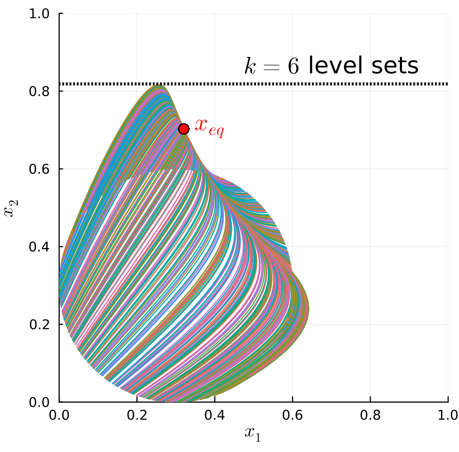
Figure 1: Trajectories and $k=6$ bounds for (19), along with position of the unique equilibrium point $x_{eq}$

V-B Three-state Rational Twist System

The second example involves a rational modification of the Twist system from Equation (37) of [30]. The three-state rational twist system is expressed in terms of matrix parameters $(A,B)$

$$A =\begin{bmatrix}-1&1&1\\ -1&0&-1\\ 0&1&-2\end{bmatrix} B =\frac{1}{2}\begin{bmatrix}-1&0&-1\\ 0&1&1\\ 1&1&0\end{bmatrix},$$ (20)

to form the expression of ($\forall i\in 1..3$):

$$\dot{x}_{i}(t) =\sum_{j=1}^{3}3B_{ij}x_{j}+\frac{A_{ij}x_{j}-4B_{ij}x_{j}^{3}}{0.5+x_{i}^{2}}.$$ (21)

The polynomial Twist dynamics in [30] lacks the $(0.5+x_{i}^{2})$ denominators. Peak estimation of (21) occurs over the state space of $X=[-1,1]^{3}$ in a time horizon of $T=6$. The initial set $X_{0}$ is the two-dimensional box $X\mid_{x_{3}=0}$. It is desired to upper-bound the peak value of $p(x)=x_{3}^{2}$ along trajectories of (21). Table II compiles computed upper-bounds of $p(x)$ along rational Twist trajectories, in the same style as in Table I. The Sum-of-Ratios program (18) returns a bound of $P^{*}\leq 1$ at degree $k=1$.

TABLE II: Bounds for Rational Twist (21)

Degree $k$	2	3	4	5	6
Sum-of-rational (18)	0.9652	0.4321	0.3590	0.3501	0.3498
Lifted (40)	1	1	1	1	1
Cleared (36)	1	1	1	1	1

A lower bound on $P^{*}$ acquired through sampling (gridding the plane $X_{0}$) is $P^{*}>0.3489$. Sampled trajectories and the $p(x)=x_{3}^{2}$ level set at the $k=6$ bound (Problem 15) for the rational Twist system are plotted in Figure 2.

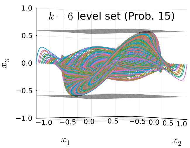
Figure 2: Trajectories and $k=6$ bound for (21)

VI Conclusion

This paper presents a scheme to perform peak estimation of rational systems. The sum-of-rational optimization technique from [26] is used to reduce the complexity of resulting moment-SOS-derived SDPs. This decomposition scheme is nonconservative if all denominator polynomials $D_{\ell}$ are positive and a compact set is considered (generating assumptions A1-A6 in the dynamical systems setting). Effectiveness of our technique was demonstrated on example systems.

Future work includes investigating methods to reduce conservatism of assumptions A1-A6 (such as if $D_{\ell}>0$ only along the graph of trajectories starting at $X_{0}$). Other options include applying our method towards rigid body kinematics, decomposing network structure in dynamics [43] through sparse sum-of-rational optimization (Theorem 3.2 of [26]), and analyzing non-ODE rational system models.

VII Acknowledgements

The authors would like to thank Mohamed Abdalmoaty, Mario Sznaier, Didier Henrion, and Matteo Tacchi for their advice and support.

Appendix A Proof of Strong Duality

This appendix will prove Theorem 14’s statement of strong duality between (14) and (15). Arguments and notation conventions from Theorem 2.6 of [44] will be used in this proof.

A Weak Duality

We will express the variables of (14) and (15) as:

$$\boldsymbol{\mu} =(\mu_{0},\mu_{p},\mu,\{\nu_{\ell}\})$$ (22a)

$$\boldsymbol{\ell} =(\gamma,v(t,x),\{q_{\ell}(t,x)\}).$$ (22b)

The variable $\boldsymbol{\mu}$ lies within the space of

$$\mathcal{X} =\mathcal{M}(X_{0})\times\mathcal{M}([0,T]\times X)^{L+1}$$ (23a)

$$\mathcal{X}^{\prime} =C(X_{0})\times C([0,T]\times X)^{L+1},$$ (23b)

of which the nonnegative subcones of the spaces are

$$\mathcal{X}_{+} =\mathcal{M}_{+}(X_{0})\times\mathcal{M}_{+}([0,T]\times X)^{L+1}$$ (23c)

$$\mathcal{X}^{\prime}_{+} =C_{+}(X_{0})\times C_{+}([0,T]\times X)^{L+1}.$$ (23d)

The variable $\boldsymbol{\ell}$ is contained within the spaces of

$$\mathcal{Y} =0\times C^{1}([0,T]\times X)^{\prime}\times\mathcal{M}([0,T]\times X)^{L}$$ (24a)

$$\mathcal{Y}^{\prime} =\mathbb{R}\times C^{1}([0,T]\times X)\times C([0,T]\times X)^{L}.$$ (24b)

In accordance with the convention of Theorem 2.6 of [44], we will also use the symbols $\mathcal{Y}_{+}=\mathcal{Y}$ and $\mathcal{Y}^{\prime}_{+}=\mathcal{Y}^{\prime}$.

The variables $\boldsymbol{\mu}$ and $\boldsymbol{\ell}$ satisfy

$$\boldsymbol{\mu} \in\mathcal{X}_{+} \boldsymbol{\ell}\in\mathcal{Y}^{\prime}.$$ (25)

The cost and constraint vectors of (14) are

$$\mathbf{c} =[0,p(x),0,\mathbf{0}]$$ (26)

$$\mathbf{b} =[1,0,\mathbf{0}].$$ (27)

The objectives of (14) and (15) respectively are

$$\langle\mathbf{c},\boldsymbol{\mu}\rangle =\langle p(x),\mu_{p}\rangle \langle\boldsymbol{\ell},\mathbf{b}\rangle =\gamma.$$ (28)

An affine map $\mathcal{A}$ with adjoint $\mathcal{A}^{\dagger}$ can be defined with

$$\mathcal{A}(\boldsymbol{\mu}) =\begin{bmatrix}\mu_{p}-\delta_{0}\otimes\mu_{0}-\mathcal{L}_{f_{0}}^{\dagger}\mu-\textstyle\sum_{\ell=1}^{\ell}(N_{\ell}\cdot\nabla_{x})^{\dagger}\nu_{\ell}\\ \mu-D^{\dagger}_{\ell}\nu_{\ell}\\ \langle 1,\mu_{0}\rangle\end{bmatrix}$$ (29a)

$$\mathcal{A}^{\prime}(\boldsymbol{\ell}) =\begin{bmatrix}\gamma-v(0,x)\\ v(t,x)-p(x)\\ \mathcal{L}_{f_{0}}v(t,x)+\textstyle\sum_{\ell=1}^{L}q_{\ell}(t,x)\\ D_{\ell}(t,x)q_{\ell}(t,x)-N_{\ell}(t,x)\cdot\nabla_{x}v(t,x)\end{bmatrix}.$$ (29b)

Problems 14 and 15 may be placed into standard conic form with weak duality [45]:

$$p^{*}_{r}= \sup_{\boldsymbol{\mu}\in\mathcal{X}_{+}}\langle\mathbf{c},\boldsymbol{\mu}\rangle \mathbf{b}-\mathcal{A}(\boldsymbol{\mu})\in\mathcal{Y}_{+}.$$ (30)

The corresponding weak dual of (30) is [45]

$$d^{*}_{r}= \inf_{\boldsymbol{\ell}\in\mathcal{Y}^{\prime}_{+}}\langle\boldsymbol{\ell},\mathbf{b}\rangle \mathcal{A}^{\prime}(\boldsymbol{\ell})-\mathbf{c}\in\mathcal{X}_{+}.$$ (31)

B Strong Duality

Strong duality under A1-A6 is attained if the following three conditions are fulfilled (sufficient condition):

• All measures in $\boldsymbol{\mu}$ that are feasible for (14) are bounded.

• There exists a feasible measure variable $\boldsymbol{\mu}$ solving (14).

• The elements of $(\mathcal{A},\mathbf{b},\mathbf{c})$ are continuous in $(t,x)$.

Requirement R1 will be proven by noting that all measures in $\boldsymbol{\mu}$ are supported on compact sets (A1), and that all feasible measures in $\boldsymbol{\mu}$ have finite mass. Requirement R2 is satisfied by choosing a feasible trajectory parameterized by $(t^{*},x_{0}^{*})$ and using the construction process from the proof of Theorem 4 to create measures $(\mu_{0},\mu_{p},\mu)$. The measures $\{\nu_{\ell}\}$ may be uniquely defined from $\mu$ by constraint (14c) as:

$$\forall\omega\in C([0,T]\times X):$$

$$\ \quad\langle\omega,\nu_{\ell}\rangle=\int_{0}^{t^{*}}\frac{\omega(t,x(t\mid x_{0}^{*}))}{D_{\ell}(t,x(t\mid x_{0}^{*}))}dt.$$ (32)

Lastly, we examine requirement R3. The vector $\mathbf{c}$ is continuous in $(t,x)$, because $p$ is continuous by A3. The vector $\mathbf{b}$ is continuous in $(t,x)$ because it is a constant. Assumption A6 ensures that $\forall\boldsymbol{\ell}\in\mathcal{Y}_{+}:$ the vector $\mathcal{A}^{\dagger}(\boldsymbol{\ell})$ is continuous in $(t,x)$ (because the product of continuous functions is continuous).

Strong duality of $p^{*}_{r}=d^{*}_{r}$ is therefore proven.

C Duality without A6

The weak dual of (10) is [4]:

$$d^{*}= \ \inf_{\gamma\in\mathbb{R}}\gamma$$ (33a)

$$\gamma\geq v(0,x) \forall x\in X_{0}$$ (33b)

$$v(t,x)\geq p(x) \forall(t,x)\in[0,T]\times X$$ (33c)

$$\mathcal{L}_{f}v(t,x)\leq 0\quad \forall(t,x)\in[0,T]\times X$$ (33d)

$$v\in C^{1}([0,T]\times X).$$ (33e)

The nonsmooth nature of $f$ in (1) violates the assumption of $(t,x)$-continuity in requirement R3. As a result, program (33) is a weak dual to Problem 3, but is not necessarily guaranteed to be a strong dual.

Appendix B Other Rational-Peak SOS Methods

This appendix presents SOS programs for peak estimation of rational functions based on clearing to common denominators [27] and by introducing new lifting variables and equality constraints [28, 29].

A Clearing to Common Denominators

Assumptions A1-A7 will be in effect for this subsection.

Let us define the polynomials $\Phi(t,x)=\prod_{\ell=1}^{L}D_{\ell}(t,x)$ and $\Phi_{\ell}(t,x)=\prod_{\ell\neq\ell^{\prime}}D_{\ell^{\prime}}(t,x)$.

The method of clearing to common denominators replaces the term

$$\mathcal{L}_{f}v(t,x)\leq 0 \forall(t,x)\in[0,T]\times X$$ (34)

from (33d) with the equivalent (under A5) expression of

$$\Phi(t,x)\mathcal{L}_{f}v(t,x)\leq 0 \forall(t,x)\in[0,T]\times X.$$ (35)

The resultant degree-$k$ SOS truncation of (33) for peak estimation under the clearing term (35) is

$$d^{*}_{c,k}= \ \inf_{\gamma\in\mathbb{R},v}\gamma$$ (36a)

$$\gamma-v(0,x)\in\Sigma[X_{0}]_{\leq 2k}$$ (36b)

$$\quad v(t,x)-p(x)\in\Sigma[([0,T]\times X)]_{\leq 2k}$$ (36c)

$$-\Phi(t,x)\mathcal{L}_{f_{0}}v(t,x)\textstyle-\sum_{\ell=1}^{L}\Phi_{\ell}(t,x)(N_{\ell}\cdot\nabla_{x}v(t,x))$$ (36d)

$$\ \qquad\in\Sigma[([0,T]\times X)]_{\leq 2k+2\lfloor(\deg\Phi-1)/2\rfloor}$$

$$v\in\mathbb{R}[t,x]_{\leq 2k}.$$ (36e)

The degree of the constraint (36d) will rapidly rise as the number of terms $L$ increases, due to the complexity of forming $\Phi(t,x)$, yielding a maximal-size PSD constraint of size $\binom{1+n+k+\lfloor(\deg\Phi-1)/2\rfloor}{1+n}$.

B Lifting Variables

This subsection will require assumptions A1-A4 and A6-A7 (but not necessarily A5). The work of [28] associates each denominator $D_{\ell}(t,x)$ to a new variable $y_{\ell}$ in the fashion of an index-1 differential-algebraic equation [46]. The support set of the lifted variable is:

$$\Omega =\{(t,x,y)\in[0,T]\times X\times\mathbb{R}^{L}\mid$$ (37)

$$\qquad\qquad\forall\ell=1\ldots L:\ y_{\ell}D_{\ell}(t,x)=1\}.$$

The set $\Omega$ will be compact under assumptions A2 and A5. The Lie derivative expression for the lifted dynamics is

$$\textstyle\mathcal{L}_{f}v(t,x)=\mathcal{L}_{f_{0}}v(t,x)+\sum_{\ell=1}^{L}y_{\ell}(N_{\ell}\cdot\nabla_{x}v(t,x)).$$ (38)

Define $Y$ as the following degree:

$$Y=\max(\deg f_{0}-1,\max_{\ell}\deg N_{\ell}).$$ (39)

The lifted-form degree-$k$ SOS program for rational peak estimation is

$$d^{*}_{y,k}= \ \inf_{\gamma\in\mathbb{R},v}\gamma$$ (40a)

$$\gamma-v(0,x)\in\Sigma[X_{0}]_{\leq 2k}$$ (40b)

$$\quad v(t,x)-p(x)\in\Sigma[([0,T]\times X)]_{\leq 2k}$$ (40c)

$$-\mathcal{L}_{f_{0}}v(t,x)\textstyle-\sum_{\ell=1}^{L}y_{\ell}(N_{\ell}\cdot\nabla_{x}v(t,x))$$ (40d)

$$\ \qquad\in\Sigma[\Omega]_{\leq 2k+2\lfloor Y/2\rfloor}$$

$$v\in\mathbb{R}[t,x]_{\leq 2k}.$$ (40e)

The Lie derivative constraint in (40d) involves $1+n+L$ variables. This results in a maximal size PSD constraint of $\binom{1+n+L+k+\lfloor Y/2\rfloor}{k+\lfloor Y/2\rfloor}$, which can be optionally reduced to $\binom{2+n+k+\lfloor Y/2\rfloor}{k+\lfloor Y/2\rfloor}$ under quotient and correlative sparsity methods at the cost of increased finite-degree conservatism.

References

[1]
J. Němcová, M. Petreczky, and J. H. van Schuppen, “Towards a system theory of rational systems,” Operator Theory, Analysis and the State Space Approach: In Honor of Rien Kaashoek, pp. 327–359, 2018.
[2]
E. Klipp, R. Herwig, A. Kowald, C. Wierling, and H. Lehrach, Systems Biology in Practice: Concepts, Implementation and Application.
John Wiley & Sons, 2005.
[3]
R. Lewis and R. Vinter, “Relaxation of optimal control problems to equivalent convex programs,” Journal of Mathematical Analysis and Applications, vol. 74, no. 2, pp. 475–493, 1980.
[4]
M. J. Cho and R. H. Stockbridge, “Linear Programming Formulation for Optimal Stopping Problems,” SIAM Journal on Control and Optimization, vol. 40, no. 6, pp. 1965–1982, 2002.
[5]
P. Mohajerin Esfahani, T. Sutter, D. Kuhn, and J. Lygeros, “From Infinite to Finite Programs: Explicit Error Bounds with Applications to Approximate Dynamic Programming,” SIAM Journal on Optimization, vol. 28, no. 3, pp. 1968–1998, 2018.
[6]
J. B. Lasserre, “Global optimization with polynomials and the problem of moments,” SIAM Journal on Optimization, vol. 11, no. 3, pp. 796–817, 2001.
[7]
D. Henrion, J. B. Lasserre, and C. Savorgnan, “Nonlinear optimal control synthesis via occupation measures,” in 2008 47th IEEE Conference on Decision and Control, pp. 4749–4754, IEEE, 2008.
[8]
G. Fantuzzi and D. Goluskin, “Bounding Extreme Events in Nonlinear Dynamics Using Convex Optimization,” SIAM Journal on Applied Dynamical Systems, vol. 19, no. 3, pp. 1823–1864, 2020.
[9]
J. Miller, D. Henrion, M. Sznaier, and M. Korda, “Peak Estimation for Uncertain and Switched Systems,” in 2021 60th IEEE Conference on Decision and Control (CDC), pp. 3222–3228, 2021.
[10]
J. Miller and M. Sznaier, “Analysis and Control of Input-Affine Dynamical Systems using Infinite-Dimensional Robust Counterparts,” 2023.
arXiv:2112.14838.
[11]
J. Miller, M. Tacchi, M. Sznaier, and A. Jasour, “Peak Value-at-Risk Estimation for Stochastic Differential Equations using Occupation Measures,” 2023.
arXiv:2303.16064.
[12]
J. Miller, M. Korda, V. Magron, and M. Sznaier, “Peak Estimation of Time Delay Systems using Occupation Measures,” 2023.
arXiv:2303.12863.
[13]
J. Miller and M. Sznaier, “Peak Estimation of Hybrid Systems with Convex Optimization,” 2023.
arXiv:2303.11490.
[14]
D. Henrion and M. Korda, “Convex computation of the region of attraction of polynomial control systems,” IEEE Trans. Automat. Contr., vol. 59, p. 297–312, Feb 2014.
[15]
A. Majumdar, R. Vasudevan, M. M. Tobenkin, and R. Tedrake, “Convex optimization of nonlinear feedback controllers via occupation measures,” The International Journal of Robotics Research, vol. 33, no. 9, pp. 1209–1230, 2014.
[16]
M. Korda, D. Henrion, and C. N. Jones, “Inner approximations of the region of attraction for polynomial dynamical systems,” IFAC Proceedings Volumes, vol. 46, no. 23, pp. 534–539, 2013.
[17]
N. Kariotoglou, S. Summers, T. Summers, M. Kamgarpour, and J. Lygeros, “Approximate dynamic programming for stochastic reachability,” in 2013 European Control Conference (ECC), pp. 584–589, IEEE, 2013.
[18]
N. Schmid and J. Lygeros, “Probabilistic Reachability and Invariance Computation of Stochastic Systems using Linear Programming,” arXiv:2211.07544, 2022.
[19]
A. Oustry, M. Tacchi, and D. Henrion, “Inner approximations of the maximal positively invariant set for polynomial dynamical systems,” IEEE Control Systems Letters, vol. 3, no. 3, pp. 733–738, 2019.
[20]
M. Korda, D. Henrion, and C. N. Jones, “Convex Computation of the Maximum Controlled Invariant Set For Polynomial Control Systems,” SICON, vol. 52, no. 5, pp. 2944–2969, 2014.
[21]
C. Schlosser and M. Korda, “Converging outer approximations to global attractors using semidefinite programming,” Automatica, vol. 134, p. 109900, 2021.
[22]
I. Tobasco, D. Goluskin, and C. R. Doering, “Optimal bounds and extremal trajectories for time averages in nonlinear dynamical systems,” Physics Letters A, vol. 382, no. 6, pp. 382–386, 2018.
[23]
L. Ambrosio, L. Caffarelli, M. G. Crandall, L. C. Evans, N. Fusco, and L. Ambrosio, “Transport equation and cauchy problem for non-smooth vector fields,” Calculus of Variations and Nonlinear Partial Differential Equations: With a historical overview by Elvira Mascolo, pp. 1–41, 2008.
[24]
L. Ambrosio and G. Crippa, “Continuity equations and ODE flows with non-smooth velocity,” Proceedings of the Royal Society of Edinburgh Section A: Mathematics, vol. 144, no. 6, pp. 1191–1244, 2014.
[25]
M. Souaiby, A. Tanwani, and D. Henrion, “Ensemble approximations for constrained dynamical systems using Liouville equation,” Automatica, vol. 149, p. 110836, 2023.
[26]
F. Bugarin, D. Henrion, and J. B. Lasserre, “Minimizing the sum of many rational functions,” Mathematical Programming Computation, vol. 8, no. 1, pp. 83–111, 2016.
[27]
J. P. Parker, D. Goluskin, and G. M. Vasil, “A study of the double pendulum using polynomial optimization,” Chaos: An Interdisciplinary Journal of Nonlinear Science, vol. 31, no. 10, 2021.
[28]
V. Magron, M. Forets, and D. Henrion, “Semidefinite approximations of invariant measures for polynomial systems,” Discrete & Continuous Dynamical Systems - B, vol. 22, no. 11, p. 1–26, 2017.
[29]
M. Newton and A. Papachristodoulou, “Rational neural network controllers,” arXiv:2307.06287, 2023.
[30]
J. Miller and M. Sznaier, “Bounding the Distance to Unsafe Sets with Convex Optimization,” IEEE Transactions on Automatic Control, pp. 1–15, 2023.
(Early Access).
[31]
D. Hilbert, “Über die Darstellung definiter Formen als Summe von Formenquadraten,” Mathematische Annalen, vol. 32, no. 3, pp. 342–350, 1888.
[32]
G. Blekherman, “There are Significantly More Nonnegative Polynomials than Sums of Squares,” Israel Journal of Mathematics, vol. 153, no. 1, pp. 355–380, 2006.
[33]
P. A. Parrilo, Structured semidefinite programs and semialgebraic geometry methods in robustness and optimization.
PhD thesis, California Institute of Technology, 2000.
[34]
M. Putinar, “Positive Polynomials on Compact Semi-algebraic Sets,” Indiana University Mathematics Journal, vol. 42, no. 3, pp. 969–984, 1993.
[35]
J. Nie and M. Schweighofer, “On the complexity of Putinar’s Positivstellensatz,” Journal of Complexity, vol. 23, no. 1, pp. 135–150, 2007.
[36]
M. Tacchi, “Convergence of Lasserre’s hierarchy: the general case,” Optimization Letters, vol. 16, no. 3, pp. 1015–1033, 2022.
[37]
S. Gribling, S. Polak, and L. Slot, “A note on the computational complexity of the moment-SOS hierarchy for polynomial optimization,” arXiv:2305.14944, 2023.
[38]
J. Wang, V. Magron, J. B. Lasserre, and N. H. A. Mai, “CS-TSSOS: Correlative and term sparsity for large-scale polynomial optimization,” ACM Transactions on Mathematical Software, vol. 48, no. 4, pp. 1–26, 2022.
[39]
J. Wang, C. Schlosser, M. Korda, and V. Magron, “Exploiting Term Sparsity in Moment-SOS Hierarchy for Dynamical Systems,” IEEE Transactions on Automatic Control, 2023.
[40]
M. Lubin, O. Dowson, J. D. Garcia, J. Huchette, B. Legat, and J. P. Vielma, “JuMP 1.0: Recent improvements to a modeling language for mathematical optimization,” Mathematical Programming Computation, 2023.
[41]
M. ApS, The MOSEK optimization toolbox for MATLAB manual. Version 10.1., 2023.
[42]
F. Blanchini, D. Breda, G. Giordano, and D. Liessi, “Michaelis–Menten networks are structurally stable,” Automatica, vol. 147, p. 110683, 2023.
[43]
C. Schlosser and M. Korda, “Sparse moment-sum-of-squares relaxations for nonlinear dynamical systems with guaranteed convergence,” arXiv preprint arXiv:2012.05572, 2020.
[44]
M. Tacchi, Moment-SOS hierarchy for large scale set approximation. Application to power systems transient stability analysis.
PhD thesis, Toulouse, INSA, 2021.
[45]
A. Barvinok, A Course in Convexity.
American Mathematical Society, 2002.
[46]
P. J. Rabier and W. C. Rheinboldt, “Theoretical and numerical analysis of differential-algebraic equations,” Handbook of Numerical Analysis, 2002.