Resource Efficient Over-the-Air Fronthaul Signaling for Uplink Cell-Free Massive MIMO Systems

Abstract

We propose a novel resource efficient analog over-the-air (OTA) computation framework to address the demanding requirements of the uplink (UL) fronthaul between the access points (APs) and the central processing unit (CPU) in cell-free massive multiple-input multiple-output (MIMO) systems. We discuss the drawbacks of the wired and wireless fronthaul solutions, and show that our proposed mechanism is efficient and scalable as the number of APs increases. We present the transmit precoding and two-phase power assignment strategies at the APs to coherently combine the signals OTA in a spectrally efficient manner. We derive the statistics of the APs’ locally available signals which enable us to to obtain the analytical expressions for the Bayesian and classical estimators of the OTA combined signals. We empirically evaluate the normalized mean square error (NMSE), symbol error rate (SER), and the coded bit error rate (BER) of our developed solution and benchmark against the state-of-the-art wired fronthaul based system.

I Introduction

Cell-free massive multiple-input multiple-output (MIMO)systems is one of the technologies envisioned to combat the low signal-to-interference-plus-noise ratio (SINR) seen by the cell-edge users in conventional multi-user MIMO systems. However, achieving the performance of fully centralized decoding with a reduced fronthaul communication overhead between the APs and the CPU is crucial to realize its full potential [1, 2]. With high-speed wired fronthaul links, it is possible to communicate all the channel state information (CSI) and the received signals from the APs to the CPU and perform the channel estimation and data detection. However, this is expensive and needs a large number of wired interconnects between the APs and the CPU. Moreover, placing the APs to suit the wired fronthaul availability may be suboptimal for the system performance. Also, when the number of APs increases, which is imperative to meet the demands of future generation communication systems, a wired fronthaul with a predefined capacity is unscalable.

In this paper, we consider an uplink cell-free massive MIMO system where multiple multi-antenna APs serve multiple single-antenna user equipments (UEs). The APs communicate with the CPU through wireless fronthaul links. To expose the main idea of this paper, we assume that each AP has a separate radio frequency (RF) chain to communicate with the CPU and uses a different frequency band for the fronthaul signaling. Our goal is to devise a spectrally efficient scheme to communicate the local information from the APs to the CPU that is sufficient to decode the data. Our proposed over-the-air (OTA)framework enables the APs to transfer their local received signals and the CSI to the CPU using the same set of resources which results in huge savings in the communication and computation overhead.

Several solutions to handle the fronthaul related issues have been studied in the literature [2, 3, 4, 5, 6]. Some of the techniques involve different cooperation levels among the distributed units, signal compression strategies to communicate between the central and distributed units, sequential wired fronthaul, etc. A millimeter wave wireless fronthaul which provides flexible deployment but requires line-of-sight (LoS) links has been explored in [7]. In [8], a sequential fronthaul referred as radio-stripes has been researched where each AP forwards the sufficient statistics to the CPU which computes the bit log-likelihood ratios (LLRs) to perform the data decoding. However, this suffers from fronthaul latency issues which worsen as the number of APs increases. To the best of our knowledge, none of the existing papers propose a systematic, spectrally efficient and scalable procedure that utilizes the wireless fronthaul architecture and OTA computation mechanism to combine the data in cell-free massive MIMO systems.

One of our objectives is obtain a function of the signals from the AP to the CPU that is sufficient to decode the information symbols. We provide an efficient and novel method of combining the data from the APs OTA [9, 10, 11, 12]. Such OTA schemes also find applications in collaborative machine learning or federated learning, where the local model updates sent by the distributed nodes are aggregated at a central node to obtain a global model. The OTA computation aims to estimate a function, $f(x_{1},\ldots,x_{L})\rightarrow\mathbb{C}$, of the signals transmitted by $L$ different nodes, $x_{l}$, $\forall l\in[L]\triangleq\{1.\ldots,L\}$. These functions can range from simple functions such as sum to complex functions such as geometric mean, maximum and minimum of function. This involves appropriate pre-processing and post-processing techniques at the APs and the CPU to achieve the centralized system performance.

We summarize the main contributions of this paper below:

1. We provide a framework to compute the sufficient statistics OTA to decode the information symbols of the UEs in a spectrally efficient manner in cell-free massive MIMO systems. It is important to note that the developed framework is scalable with the number of APs.

2. We develop transmit precoding and two-phase power assignment schemes to combine the sufficient statistics OTA which leads to reduced communication and computation load on the wireless fronthaul.

3. We derive the first and second order statistics of the locally available sufficient statistics i.e., the Gramian of the channel matrix and the matched filter outputs at the APs.

4. We provide closed-form analytical expressions for the least squares (LS) and linear minimum mean-square error (LMMSE) estimators of the sufficient statistics.

5. We numerically evaluate the NMSE, SER, and the coded BER performances of the proposed solution and benchmark against the state-of-the-art.

II System Model and Preliminaries

We consider the UL of a cell-free massive MIMO system with $K$ single-antenna UEs transmitting data to $L$ APs with $N$ receive antennas each. We assume that $LN\leavevmode\nobreak\ >\leavevmode\nobreak\ K$. Each AP transfers a linear transformation of its received signal to an $M$ receive antenna CPU which performs the UL data decoding. We assume that the APs use a different frequency band with a separate RF chain and a dedicated wireless fronthaul link to communicate with the CPU. We use a quasi-static block fading model for all the wireless channels in the network. We denote the channel between UE $k$ and AP $l$ by $\mathbf{h}_{{kl}}\in\mathbb{C}^{N\times 1}$ and the channel between AP $l$ and the CPU by $\mathbf{G}_{{l}}\in\mathbb{C}^{M\times N}$.

The received signal at the $l$-th AP during the UL data transmission phase is given by

$$\mathbf{y}_{l}=\sqrt{\rho_{\rm ul}}\mathbf{H}_{{l}}\mathbf{s}+\mathbf{n}_{l}\in\mathbb{C}^{N\times 1}$$ (1)

where $\rho_{\rm ul}$ is the UL signal-to-noise ratio (SNR) of each UE, $\mathbf{H}_{{l}}=\left[\mathbf{h}_{{1l}},\mathbf{h}_{{2l}},\ldots,\mathbf{h}_{{Kl}}\right]\in\mathbb{C}^{N\times K}$ is the channel matrix whose columns are independent of each other and distributed as circularly symmetrically complex Gaussian $\mathbf{h}_{{kl}}\sim\mathcal{CN}{(\mathbf{0},\mathbf{R}_{kl})}$, $k\in[K]$, $\mathbf{s}=[s_{1},s_{2},\ldots,s_{K}]^{T}\in\mathbb{C}^{K\times 1}$, $s_{k}$ is the transmit symbol of the UE $k$, and $\mathbf{n}_{l}\sim\mathcal{CN}{(\mathbf{0},\mathbf{I}_{N})}$ is the circularly symmetric additive white complex Gaussian noise at the AP $l$ where $\mathbf{I}_{N}$ denotes an identity matrix of dimension $N$. To expose the concept of the OTA combining in cell-free massive MIMO systems, we assume that the APs have perfect CSI of the UEs.

In a conventional system, each AP has to send $\mathbf{y}_{l}$ and $\mathbf{H}_{{l}}$, $\ l\in[L]$, to the CPU using orthogonal resources to decode the data, which leads to a huge fronthaul communication overhead of $(LN+LNK)$ complex channel uses. However, by preprocessing $\mathbf{y}_{l}$ and $\mathbf{H}_{{l}}$ at the APs and using efficient analog OTA combining methods in the wireless fronthaul, we can achieve the performance of a centralized decoding method with a reduced fronthaul communication overhead. One potential way to do this is to send the local sufficient statistics: the Gramian matrix $\mathbf{T}_{l}^{(1)}\triangleq\mathbf{H}_{l}^{H}\mathbf{H}_{l}$ and the matched filter output $\mathbf{t}_{l}^{(2)}\triangleq\mathbf{H}_{l}^{H}\mathbf{y}_{l}$ rather than $\mathbf{H}_{l}$ and $\mathbf{y}_{l}$, $l\in[L]$ from the APs to the CPU. This is because, any linear or non-linear multiuser detector employed at the CPU needs only the sum of the locally obtained sufficient statistics

$$\mathbf{T}^{(1)}=\sum_{l=1}^{L}\mathbf{T}_{l}^{(1)}\quad\text{and}\quad\mathbf{t}^{(2)}=\sum_{l=1}^{L}\mathbf{t}_{l}^{(2)}$$ (2)

to decode the data symbols. For example, the LMMSE detector depends only on the terms in (2) as follows:

$$\widehat{\mathbf{s}}=\sqrt{\rho_{\rm ul}}\left(\rho_{\rm ul}\mathbf{T}^{(1)}+\mathbf{I}_{K}\right)^{-1}\mathbf{t}^{(2)}.$$ (3)

Moreover, when we utilize the wireless properties to compute (2) OTA, the solution scales well with the number of APs.

Each AP preprocesses and sends its locally obtained sufficient statistics to the CPU in a non-orthogonal manner. We divide this into two phases: the $l$-th AP transmits $\mathbf{T}_{l}^{(1)}$ and $\mathbf{t}_{l}^{(2)}$ in the first and second phases, respectively. We assume that $N\geq M$ and each AP transmits $M$ complex symbols per channel use. Further, observe that $\mathbf{T}_{l}^{(1)}$ is a Hermitian symmetric matrix and it is enough to transmit either its upper or lower triangular parts i.e., AP $l$ transmits $\mathbf{x}_{l}^{(1)}$ given in (4) in the next page, which is a vectorized form of the upper triangular part of $\mathbf{T}_{l}^{(1)}$. This translates to $M_{1}=\left\lceil\frac{K(K+1)}{2M}\right\rceil$ transmissions in the first phase. In the second phase, $M_{2}=\left\lceil\frac{\tau_{\rm u}K}{M}\right\rceil$ transmissions are needed, where $\tau_{\rm u}$ is the number of channel uses by each UE to transmit its UL data.

$$\mathbf{x}_{l}^{(1)}={\begin{bmatrix}\left\|\mathbf{h}_{1l}\right\|^{2}&\mathbf{h}_{1l}^{H}\mathbf{h}_{2l}&\cdots&\mathbf{h}_{1l}^{H}\mathbf{h}_{Kl}&\left\|\mathbf{h}_{2l}\right\|^{2}&\mathbf{h}_{2l}^{H}\mathbf{h}_{3l}&\cdots&\mathbf{h}_{2l}^{H}\mathbf{h}_{Kl}&\cdots&\left\|\mathbf{h}_{Kl}\right\|^{2}\end{bmatrix}^{T}}.$$ (4)

 

In the second phase, the $l$-th AP transmits

$$\mathbf{x}_{l}^{(2)}=\begin{bmatrix}{\mathbf{t}_{l,1}^{(2)}}^{T}&{\mathbf{t}_{l,2}^{(2)}}^{T}&\cdots&{\mathbf{t}_{l,\tau_{\rm u}}^{(2)}}^{T}\end{bmatrix}^{T},$$ (5)

where the second index in the subscript of $\mathbf{t}_{l,t}^{(2)}$ denotes the $t$-th transmission interval of the matched filter output $\mathbf{t}_{l}^{(2)}$. We next describe the methods to combine the sufficient statistics.

III Over-the-Air Combining Schemes

We propose OTA schemes to coherently combine the local sufficient statistics transmitted by the APs to the CPU. To start with, let us denote the transmit precoder of the $l$-th AP by $\mathbf{W}_{l}\in\mathbb{C}^{N\times M}$. The received signal at the CPU is given by

$$\mathbf{Z}^{(i)}=\sum_{l=1}^{L}\sqrt{\rho_{\rm c}}\mathbf{G}_{l}^{H}\mathbf{W}_{l}\bar{\mathbf{X}}_{l}^{(i)}+\mathbf{E}^{(i)}\in\mathbb{C}^{M\times M_{i}},$$ (6)

where $i\in\{1,2\}$ denotes the index of the two transmission phases of the APs to send their local sufficient statistics, $\mathbf{G}_{l}^{H}\in\mathbb{C}^{M\times N}$ is the channel between the $l$-th AP and the CPU, $\rho_{\rm c}$ is a common power assignment scaling factor of the APs to satisfy the average transmit power constraint, $\mathbf{E}^{(i)}$ is the additive noise whose columns are complex Gaussian distributed with mean $\mathbf{0}_{M}$ and covariance $\mathbf{I}_{M}$. The transmit signal matrix of the $l$-th AP denoted by $\bar{\mathbf{X}}_{l}^{(i)}$ is

$$\bar{\mathbf{X}}_{l}^{(i)}=\begin{bmatrix}\bar{\mathbf{x}}_{l,1}^{(i)}&\ldots&\bar{\mathbf{x}}_{l,M_{i}}^{(i)}\end{bmatrix}\in\mathbb{C}^{M\times M_{i}},\quad i\in\{1,2\},$$ (7)

where $\bar{\mathbf{x}}_{l,m}^{(i)}\in\mathbb{C}^{M\times 1}$ corresponds to the $((m-1)M+1)$-th to the $mM$-th entries of $\mathbf{x}_{l}^{(i)}$ given in (4) and (5). Note that $\bar{\mathbf{x}}_{l,M_{i}}^{(i)}$, $i\in\{1,2\}$ are zero padded if $M$ is not an integer multiple of $\frac{K(K+1)}{2}$ and $\tau_{\rm u}K$ for $i=1$ and $i=2$, respectively.

To minimize the fronthaul load, we consider the case where the CPU does not need to have any knowledge of the CSI of the APs. The APs obtain their respective CSI using downlink training from the CPU. Moreover, for ease of exposition and also because APs and the CPU are stationary, we assume perfect CSI at the APs. To obtain the sum of the local sufficient statistics, each AP first offsets the effect of $\mathbf{G}_{l}$, $l\in[L]$. In this paper, we assume that all the channels between the APs and the CPU have full column rank. In future generation wireless systems, the APs can be low-cost nodes deployed by the network planners based on the requirements and therefore the channels to the CPU undergo rich scattering which justifies the full column rank assumption. We will deal with other channel models in the journal version of this paper. We set the number of antennas at the CPU less than or equal to that of the APs ($M\leq N$) and use a local zero forcing (ZF) precoder at each AP as $\mathbf{W}_{l}=\mathbf{G}_{l}\left(\mathbf{G}_{l}^{H}\mathbf{G}_{l}\right)^{-1}\in\mathbb{C}^{N\times M}$, $l\in[L]$. As these channels are relatively time invariant, each AP computes the transmit precoder once and reuses it till the channels change.

We recall that our goal is to compute $\sum_{l=1}^{L}\bar{\mathbf{X}}_{l}^{(i)}$, and ZF precoding only cancels the effects of the channels between the APs and the CPU. However, any unequal power scaling at the APs will result in residual scaling factors which are impossible to be removed OTA. To circumvent this power scaling problem, we propose an average transmit power assignment strategy at the APs to communicate with the CPU. The total energy expended by the $l$-th AP during the $M_{1}$ and $M_{2}$ symbol intervals is:

$$\Omega_{l}^{(i)} =\rho_{\rm c}^{(i)}\,\sum_{t=1}^{M_{i}}\mathbb{E}\left\{\left\|\mathbf{W}_{l}\bar{\mathbf{x}}_{l,t}^{(i)}\right\|^{2}\right\},$$

$$=\rho_{\rm c}^{(i)}\,{\rm tr}\left(\left(\mathbf{I}_{M_{i}}\otimes\mathbb{E}\left\{\mathbf{W}_{l}^{H}\mathbf{W}_{l}\right\}\right)\mathbb{E}\left\{{\mathbf{x}}_{l}^{(i)}{{\mathbf{x}}_{l}^{(i)^{H}}}\right\}\right),$$ (8)

where $i\in\{1,2\}$ and $\otimes$ denotes the matrix Kronecker product operator. We use two separate scaling mechanisms for transmitting the Gramian and the matched filter outputs from the APs to the CPU to accommodate for the differences in their dynamic ranges. Note that the matched filter outputs have $\rho_{\rm ul}$ embedded in them which changes their dynamic ranges compared to that of the Gramian matrices. Therefore, it is imperative to employ this two-phase power assignment strategy to obtain good system performance.

The values of $\Omega_{l}^{(1)}$ and $\Omega_{l}^{(2)}$ can be computed using the corresponding mean and covariance matrices of the sufficient statistics which we will discuss subsequently. Therefore, the average transmit power of the $l$-th AP to transmit the Gramian matrices and the matched filter outputs of one coherence interval is

$$P_{l}^{(i)}=\frac{\Omega_{l}^{(i)}}{M_{i}},\qquad i\in\{1,2\}.$$ (9)

Now, let us denote the maximum average power constraint by $P_{\rm max}$ for all the APs. We propose a low overhead feedback mechanism to compute the common power scaling factors $\rho_{\rm c}^{(1)}$ and $\rho_{\rm c}^{(2)}$ at the CPU (to assist in the coherent addition of the sufficient statistics at the CPU) and broadcast it to the APs via a common control channel to satisfy the average transmit power constraint.

For $i\in\{1,2\}$, each AP sets $\rho_{\rm c}^{(i)}$ equal to $1$, computes the scalar value in (9) using the locally available statistics and conveys it to the CPU using a dedicated control channel. This can be done after the pilot transmissions from the CPU to the APs occasionally. Upon receiving $\{P_{1}^{(i)},\ldots,P_{L}^{(i)}\}$, $i\in\{1,2\}$, the CPU obtains the indices of the APs which violate the constraint. Let us include these indices in the sets $\mathcal{V}^{(i)}=\{i_{1}^{(i)},\ldots,i_{L^{\prime(i)}}^{(i)}\}\subseteq\{1,\ldots,L\}$, where $L^{\prime(i)}$, $i\in\{1,2\}$, is the number of APs in it. Then the scaling factors are computed as

$$\rho_{\rm c}^{(i)}=\frac{P_{\rm max}}{\max_{i\in\mathcal{V}}P_{i}^{(i)}},\qquad i\in\{1,2\}.$$ (10)

This ensures that every AP satisfies its average transmit power constraint and is necessary to add the sufficient statistics coherently at the CPU.

Substituting $\mathbf{W}_{l}=\mathbf{G}_{l}\left(\mathbf{G}_{l}^{H}\mathbf{G}_{l}\right)^{-1}$ in to the received signal (6), the CPU receives the following signal

$$\mathbf{Z}^{(i)}\triangleq\begin{bmatrix}\mathbf{z}_{1}^{(i)}&\ldots&\mathbf{z}_{M_{i}}^{(i)}\end{bmatrix}=\sqrt{\rho_{\rm c}^{(i)}}\sum_{l=1}^{L}\bar{\mathbf{X}}_{l}^{(i)}+\mathbf{E}^{(i)},$$ (11)

where $i\in\{1,2\}$, $\{\mathbf{z}_{1}^{(i)},\ldots,\mathbf{z}_{M_{i}}^{(i)}\}$ are the columns of $\mathbf{Z}^{(i)}$ and $\bar{\mathbf{X}}_{l}^{(i)}$ is given in (7).

Now we provide two estimators to obtain the sum of the local sufficient statistics at the CPU: Bayesian and classical estimators. To do that, we first derive the mean and covariance of the sufficient statistics below.

III-A Derivation of the Statistics of the Sufficient Statistics

First, note that the channels between the AP and the UEs are independent of each other which means that $\{\mathbf{x}_{l}^{(1)}\}$, $l\in[L]$ are statistically independent. Therefore, the mean $\bm{\mu}^{(1)}$ and the covariance matrix $\mathbf{C}^{(1)}$ of $\mathbf{x}^{(1)}=\sum_{l=1}^{L}\mathbf{x}_{l}^{(1)}$ are given by

$$\bm{\mu}^{(1)}=\sum_{l=1}^{L}\bm{\mu}_{l}^{(1)},\qquad\mathbf{C}^{(1)}=\sum_{l=1}^{L}\mathbf{C}_{l}^{(1)},$$ (12)

where $\bm{\mu}_{l}^{(1)}$ and $\mathbf{C}_{l}^{(1)}$ are the mean and covariance matrix of $\mathbf{x}_{l}^{(1)}$, $l\in[L]$. To compute $\bm{\mu}_{l}^{(1)}$ and $\mathbf{C}_{l}^{(1)}$ when the channels between the UEs and the APs undergo correlated Rayleigh fading, we need the statistics of the sum of chi-squared and product of complex Gaussian random variables. We compute them in closed form here. The nonzero entries of $\bm{\mu}_{l}^{(1)}$ and $\mathbf{C}_{l}^{(1)}$ are governed by the following indexing equations: For a given $j\in[K]$ and $j^{\prime}\in\{j,\ldots,K\}$, the non-zero $n$-th entry of $\bm{\mu}_{l}^{(1)}$ and non-zero $(n^{\prime},n^{\prime})$-th diagonal entry of $\mathbf{C}_{l}^{(1)}$ are at the indices $n=(K-0.5j)(j-1)+j$ and $n^{\prime}=(K-0.5j)(j-1)+j^{\prime}$ which are given by

$$\bm{\mu}_{l}^{(1)}[n]={\rm tr}\left(\mathbf{R}_{jl}\right),\quad\mathbf{C}_{l}^{(1)}[n^{\prime},n^{\prime}]={\rm tr}\left(\mathbf{R}_{jl}\mathbf{R}_{j^{\prime}l}\right)\$$ (13)

For $i=2$, to compute the mean and covariance of each column in (7), we focus on the term $\sum_{l=1}^{L}\mathbf{t}_{l,t}^{(2)}$ i.e., the matched filter output at time $t\in[\tau_{u}]$. For $t\neq t^{\prime}$, $\mathbf{t}_{l,t}^{(2)}$ and $\mathbf{t}_{l,t^{\prime}}^{(2)}$ are uncorrelated and for $l\neq l^{\prime}$, $\mathbf{t}_{l,t}^{(2)}$ and $\mathbf{t}_{l^{\prime},t}^{(2)}$ are correlated. Therefore, to compute the mean and covariance of $\sum_{l=1}^{L}\mathbf{t}_{l,t}^{(2)}$, we need the mean $\bm{\mu}_{l,t}^{(2)}$, the covariance matrix $\mathbf{C}_{l,t}^{(2)}$ of $\mathbf{t}_{l,t}^{(2)}$ and also the cross-covariance matrix $\mathbf{C}_{ll^{\prime},t}^{(2)}$ between $\mathbf{t}_{l,t}^{(2)}$ and $\mathbf{t}_{l^{\prime},t}^{(2)}$. We can compute the mean to be zero because $\bm{\mu}_{l,t}^{(2)}=\mathbf{0}$ for any $l$ and $t$. The covariance $\mathbf{C}_{t}^{(2)}$ of $\sum_{l=1}^{L}\mathbf{t}_{l,t}^{(2)}$ is given by

$$\mathbf{C}_{t}^{(2)}=\sum_{l=1}^{L}\mathbf{C}_{l,t}^{(2)}+\sum_{l=1}^{L}\sum_{\begin{subarray}{c}l^{\prime}=1,l^{\prime}\neq l\end{subarray}}^{L}\mathbf{C}_{ll^{\prime},t}^{(2)}.$$ (14)

For correlated Rayleigh fading, we derive the closed form expressions as

$$\mathbf{C}_{l,t}^{(2)} =\rho_{\rm ul}\mathbb{E}\left\{\left(\mathbf{H}_{l}^{H}\mathbf{H}_{l}\right)^{2}\right\}+\mathbb{E}\left\{\left(\mathbf{H}_{l}^{H}\mathbf{H}_{l}\right)\right\},$$ (15)

$$\mathbf{C}_{ll^{\prime},t}^{(2)} =\rho_{\rm ul}\mathbb{E}\left\{\left(\mathbf{H}_{l}^{H}\mathbf{H}_{l}\right)\right\}\mathbb{E}\left\{\left(\mathbf{H}_{l^{\prime}}^{H}\mathbf{H}_{l^{\prime}}\right)\right\}.$$ (16)

where $\mathbb{E}\{\left(\mathbf{H}_{l}^{H}\mathbf{H}_{l}\right)\}={\rm diag}\left({\rm tr}\left(\mathbf{R}_{1l}\right),\ldots,{\rm tr}\left(\mathbf{R}_{Kl}\right)\right)$, and $\mathbb{E}\{\left(\mathbf{H}_{l}^{H}\mathbf{H}_{l}\right)^{2}\}$ is a diagonal matrix whose $k$-th diagonal entry is ${\rm tr}\left(\mathbf{R}_{kl}\right)^{2}+{\rm tr}\left(\mathbf{R}_{kl}\sum_{k^{\prime}=1}^{K}\mathbf{R}_{k^{\prime}l}\right)$. Finally, $\mathbb{E}\{\mathbf{W}_{l}^{H}\mathbf{W}_{l}\}$ can be evaluated numerically. With the mean, covariance and cross covariance matrices of the sum of the sufficient statistics, we present the estimators to obtain them below.

III-B LMMSE and LS Estimators

With a prior on the sufficient statistics, the CPU considers a LMMSE estimator of $\sum_{l=1}^{L}\bar{\mathbf{X}}_{l}^{(i)}$, $i\in\{1,2\}$. For convenience, let us denote the mean and covariance of $\sum_{l=1}^{L}\bar{\mathbf{x}}_{l,m}^{(i)}$. $m\in[M_{i}],\ i\in\{1,2\}$ by $\bar{\bm{\mu}}_{m}^{(i)}$ and $\bar{\mathbf{C}}_{m}^{(i)}$, respectively. Note that $\bar{\bm{\mu}}_{m}^{(i)}$ and $\bar{\mathbf{C}}_{m}^{(i)}$ can be obtained by selecting the appropriate entries from the mean and covariance matrices derived in (12) and (14). Then, the LMMSE estimate of $\sum_{l=1}^{L}\bar{\mathbf{x}}_{l,m}^{(i)}$, $i\in\{1,2\}$ (denoted by $\widehat{\bar{\mathbf{x}}}_{m}^{(i)}$), for $m\in[M_{i}],\ i\in\{1,2\}$ is

$$\widehat{\bar{\mathbf{x}}}_{m}^{(i)}=\bar{\bm{\mu}}_{m}^{(i)}+\sqrt{\rho_{\rm c}^{(i)}}\bar{\mathbf{C}}_{m}^{(i)} \left({\rho_{\rm c}^{(i)}}\bar{\mathbf{C}}_{m}^{(i)}+\mathbf{I}_{M}\right)^{-1}$$

$$\times\left(\mathbf{z}_{m}^{(i)}-\sqrt{\rho_{\rm c}^{(i)}}\bar{\bm{\mu}}_{m}^{(i)}\right).$$ (17)

In the case when the CPU does not have any prior information of the sufficient statistics, the CPU implements the minimum variance unbiased (MVU) estimator

$$\widehat{\bar{\mathbf{x}}}_{m}^{(i)}=\left({\rho_{\rm c}^{(i)}}\right)^{-\frac{1}{2}}\mathbf{z}_{m}^{(i)},$$ (18)

which is also efficient [14]. In this case, the MVU estimator is also the LS estimator. Finally, the CPU computes the Gramian matrix $\widehat{\mathbf{H}^{H}\mathbf{H}}$ and the matched filter output $\widehat{\mathbf{H}^{H}\mathbf{y}}$ in the two phases using the estimated sum of the sufficient statistics.

IV Data Detection

We use the sum of the sufficient statistics obtained during the two phases to detect the information symbols of the UEs. Let us denote $\mathbf{y}=\begin{bmatrix}\mathbf{y}_{1}^{H}&\ldots&\mathbf{y}_{L}^{H}\end{bmatrix}^{H}\in\mathbb{C}^{LN}$, $\mathbf{H}=[\mathbf{H}_{{l}}^{H},\ldots,\mathbf{H}_{{L}}^{H}]^{H}\in\mathbb{C}^{LN\times K}$. We use the following data detectors for our numerical evaluation. Note that our developed solution is equally applicable to any data detector.

IV-A Linear Detectors

We present the centralized LMMSE and LS estimates of the data symbols here:

$$\widehat{\mathbf{s}}_{\text{\lx@glossaries@gls@link{main}{lmmse}{\leavevmode LMMSE}}} =\sqrt{\rho_{\rm ul}}\left(\rho_{\rm ul}\mathbf{H}^{H}\mathbf{H}+\mathbf{I}_{K}\right)^{-1}\mathbf{H}^{H}\mathbf{y}$$ (19)

$$\approx\sqrt{\rho_{\rm ul}}\left(\rho_{\rm ul}\widehat{\mathbf{H}^{H}\mathbf{H}}+\mathbf{I}_{K}\right)^{-1}\widehat{\mathbf{H}^{H}\mathbf{y}}.$$

and

$$\widehat{\mathbf{s}}_{\text{LS}}=\rho_{\rm ul}^{-1/2}\left(\widehat{\mathbf{H}^{H}\mathbf{H}}\right)^{-1}\widehat{\mathbf{H}^{H}\mathbf{y}},$$ (20)

respectively.

IV-B Maximum aposteriori (MAP) Detector

The MAP detector outputs

$$\widehat{\mathbf{s}}_{\text{MAP}} =\operatorname*{arg\,max}_{\mathbf{s}\in\mathcal{S}}\left\|\mathbf{y}-\sqrt{\rho_{\rm ul}}\mathbf{H}\mathbf{s}\right\|=\operatorname*{arg\,max}_{\mathbf{s}\in\mathcal{S}}\left\|\overline{\mathbf{y}}-\sqrt{\rho_{\rm ul}}\overline{\mathbf{H}}\mathbf{s}\right\|$$

$$\approx\operatorname*{arg\,max}_{\mathbf{s}\in\mathcal{S}}\left\|\widehat{\overline{\mathbf{y}}}-\sqrt{\rho_{\rm ul}}\widehat{\overline{\mathbf{H}}}\mathbf{s}\right\|,$$

where ${\overline{\mathbf{H}}}=\left({\mathbf{H}^{H}\mathbf{H}}\right)^{\frac{1}{2}}$, ${\overline{\mathbf{y}}}=\left({\mathbf{H}^{H}\mathbf{H}}\right)^{-\frac{1}{2}}$$\mathbf{H}^{H}\mathbf{y}$,
$\widehat{\overline{\mathbf{H}}}=\left(\widehat{\mathbf{H}^{H}\mathbf{H}}\right)^{\frac{1}{2}}$ and $\widehat{\overline{\mathbf{y}}}=\left(\widehat{\mathbf{H}^{H}\mathbf{H}}\right)^{-\frac{1}{2}}\widehat{\mathbf{H}^{H}\mathbf{y}}$ and $\mathcal{S}$ is the constellation set.

IV-C Soft-output Detection

We can also use soft detection methods to compute the bit LLRs as:

$$\mathcal{L}\left(b_{i}\rvert\widehat{\mathbf{H}^{H}\mathbf{y}},\widehat{\mathbf{H}^{H}\mathbf{H}}\right)\approx\ln\left(\frac{\sum_{\mathbf{s}:b_{i}(\mathbf{s})=1}e^{-\left\|\widehat{\overline{\mathbf{y}}}-\sqrt{\rho_{\rm ul}}\widehat{\overline{\mathbf{H}}}\mathbf{s}\right\|^{2}}}{\sum_{\mathbf{s}:b_{i}(\mathbf{s})=0}e^{-\left\|\widehat{\overline{\mathbf{y}}}-\sqrt{\rho_{\rm ul}}\widehat{\overline{\mathbf{H}}}\mathbf{s}\right\|^{2}}}\right)$$ (21)

where $\mathcal{L}(b_{i})=\ln({\rm Pr}(b_{i}=1)/{\rm Pr}(b_{i}=0))$, and the notation $\mathbf{s}:b_{i}(\mathbf{s})=\alpha$ means the set of all vectors $\mathbf{s}$ for which the $i$-th bit is $\alpha$ i.e., $b_{i}(\mathbf{s})=\alpha$. After computing the LLRs, we can input them to a channel decoder in case of a coded communication system.

V Numerical Results

In this section, we evaluate the performance of the proposed OTA framework using the following simulation setup: The locations of the UEs are uniformly distributed in a square area of $200\leavevmode\nobreak\ {\rm m}\times 200\leavevmode\nobreak\ {\rm m}$ whereas the locations of APs and the CPU are fixed around the center of the square. We further position the antennas of the APs and the CPU at a height of $5\leavevmode\nobreak\ {\rm m}$ above the UEs. We consider a 3GPP urban microcell channel propagation model with a carrier frequency of $2$ GHz [15, Table B.1.2.1-1]. The large-scale fading coefficient is determined by: $\beta_{kl}\triangleq{{\rm tr}\left(\mathbf{R}_{kl}\right)}/{N}=-30.5-36.7\log_{10}({\rm d}_{kl}/{1{\rm m}})$, where ${\rm d}_{kl}$ represents the distance between the AP $l$ and the UE $k$. The noise power spectral density, bandwidth and the noise figure are set to $-174\leavevmode\nobreak\ {\rm dBm/Hz}$, $1\leavevmode\nobreak\ {\rm MHz}$ and $5\leavevmode\nobreak\ {\rm dB}$, respectively. We set the values of $L$, $K$, $N$, and $M$ to $16$, $8$, $5$, and $4$, respectively. The APs and the CPU use uniform linear array antennas with half-wavelength antenna spacing. The spatial correlation matrices, $\mathbf{R}_{kl},\ k\in[K],l\in[L]$ are modeled as uncorrelated channels. With spatially uncorrelated channels between APs and the CPU, we can compute $\mathbb{E}\{\mathbf{W}_{l}^{H}\mathbf{W}_{l}\}$ using closed form expressions [16]. We denote $\rho_{\rm ul}=\frac{P_{\rm ul}\beta_{\rm avg}}{BN_{0}}$, where $P_{\rm ul}$ is the transmit power of the UEs, $B$ is the bandwidth, $N_{0}$ is the additive white noise power spectral density, and $\beta_{\rm avg}$ is the average path loss of a UE.

In Fig. 1, we plot the NMSE in ${\rm dB}$ of the estimated Gramian and matched filter outputs (defined as $\frac{\mathbb{E}\{\left\|\mathbf{x}-\widehat{\mathbf{x}}\right\|^{2}\}}{\mathbb{E}\{\left\|\mathbf{x}\right\|\}^{2}}$, where $\widehat{\mathbf{x}}$ is the estimate of a random vector $\mathbf{x}$ and the expecation operator performs an empirical average of at least $10^{5}$ Monte carlo runs.) as a function of $\rho_{\rm ul}$. We compare the LMMSE and LS estimators in (III-B) and (18) when $P_{\rm max}$ is set to $1$ W and $5$ W. We observe that the performance difference between the LS and the LMMSE estimators is negligible and both of them achieve an NMSE of less than $-45$ dB even when $P_{\rm max}$ is set to only $1$ W. Note that the NMSE of the Gramian estimate is a constant for any value of $\rho_{\rm ul}$. The Gramian matrices transmitted by the APs during the first phase are independent of the transmit SNRs of the UEs which results in a constant NMSE. However, as $P_{\rm max}$ increases, the NMSE of the Gramian matrix decreases. On the other hand, the matched filter outputs transmitted by the APs and the power scaling factor $\rho_{\rm c}^{(2)}$ are dependent on $\rho_{\rm ul}$ which impacts their mean square error (MSE) performance. However, when we normalize the MSE with the expected power of the matched filter outputs, it results in almost a constant line at higher transmit SNRs as shown in the Fig. 1.

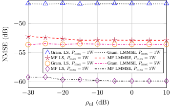
Figure 1: NMSE of the estimated sufficient statistics as a function of $\rho_{\rm ul}$.

In Fig. 2, we show the SER performance of the LMMSE data detector as a function of $\rho_{\rm ul}$ when the UEs transmit 4-quadrature amplitude modulation (QAM) modulated symbols to the APs. The sufficient statistics are obtained using LS and LMMSE estimators. An initial symbol estimate is obtained using the LMMSE detector in (19) followed by a nearest-neighbor approximation to detect the data symbols. We observe that the SER performance with the sufficient statistics estimated through LS and LMMSE estimators almost matches that of a cell-free massive MIMO system with centralized decoding upto around $-15\leavevmode\nobreak\ {\rm dB}$ with $P_{\rm max}=5\leavevmode\nobreak\ {\rm W}$. An interesting observation is that the SER obtained by the OTA methods reaches an error floor beyond a particular value of $\rho_{\rm ul}$. Moreover, as $P_{\rm max}$ increases, the value of $\rho_{\rm ul}$ at which the error floor happens also increases. This is because, as $\rho_{\rm ul}$ increases, the scaling factor $\rho_{\rm c}^{(2)}$ to satisfy the average transmit power constraint during the transmission of the matched filter outputs from the APs decreases. This leads to a saturation effect in the receive SNR at the CPU resulting in an error floor. Further, as $P_{\rm max}$ increases, the saturation effect of the receive SNR at the CPU occurs at a higher value of $\rho_{\rm ul}$.

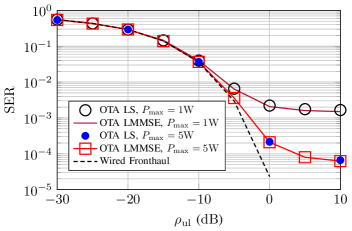
Figure 2: SER of the detected data symbols as a function of $\rho_{\rm ul}$.

Figure 3: SER of the detected data symbols as a function of $P_{\rm max}$.

We plot the SER as a function of $P_{\rm max}$ in the Fig. 3 when $\rho_{\rm ul}$ is set to $\{-4,-3\}\leavevmode\nobreak\ {\rm dB}$. We observe that as $P_{\rm max}$ increases, the reliability of the wireless links between the APs and the CPU improves which leads to reduction in the SER for both the values of $\rho_{\rm ul}$. Moreover, the performance difference between the LS, LMMSE estimators and a wired fronthaul is negligible beyond a $P_{\rm max}$ of around $30$ dB. This also confirms our earlier observation that increasing $P_{\rm max}$ alleviates the error floor issue seen in the Fig. 2. This shows that there is a performance-to-power consumption trade-off and appropriate selection of the system and transmit parameters can be done based on the system design requirements.

In Fig. 4, we plot the coded BER as a function of $\frac{{\rm E_{b}}\beta_{\rm avg}}{N_{0}}$ when $P_{\rm max}$ is set to $1$ W and $5$ W. We employ an LDPC error correcting code of rate ${\rm R_{c}}=1/2$ and length $1944$ from the IEEE 802.11-2020 wireless local-area network (WLAN) standard [17]. We set $K$, $N$ and $M$ to $4$, $5$, and $3$, respectively. The symbol energy ${\rm E_{s}}$ is related to the bit energy ${\rm E_{b}}$ as ${\rm E_{s}}={\rm E_{b}}\log_{2}(|\mathcal{S}|){\rm R_{c}}$, where $|\mathcal{S}|$ is the cardinality of the constellation set $\mathcal{S}$. We have used a max-log approximation of (21) to compute the posterior bit LLRs and adopted the sphere decoding algorithm to obtain them efficiently. We have used the LMMSE estimator to obtain the sufficient statistics and benchmarked the coded BER performance with a centralized wired fronthaul based system. We observe that channel coding not only reduces the performance gap between the wireless and wired fronthaul based systems, but also assists in mitigating the error floor issue seen in the Fig. 2. Note that there will be an error floor at much higher SNRs which may be beyond the region of our interest.

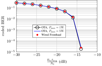
Figure 4: Coded BER as a function of SNR. Sphere decoder is used to obtain the posterior bit LLRs.

VI Conclusions

In this paper, we presented a novel scalable framework to combine the locally obtained sufficient statistics at the APs OTA in cell-free massive MIMO systems. We presented the LS and LMMSE estimators to obtain the sum of the sufficient statistics using the closed-form expressions of the statistics of the sufficient statistics for the Gaussian channel case. We also developed the transmit precoding and two-phase power assignment mechanisms to coherently combine the sufficient statistics OTA. We empirically observed that the NMSE, SER and coded BER performances of the developed OTA framework closely matches that of a wired fronthaul based cell-free massive MIMO system. Our numerical results show that the developed OTA framework is a feasible and scalable approach to reduce the communication and computational overhead associated with a wired fronthaul based cell-free massive MIMO system.

References

- [1] Ö. T. Demir, E. Björnson, and L. Sanguinetti, “Foundations of user-centric cell-free massive MIMO,” Foundations and Trends® in Signal Processing, vol. 14, no. 3-4, pp. 162–472, 2021.
- [2] H. A. Ammar, R. Adve, S. Shahbazpanahi, G. Boudreau, and K. V. Srinivas, “User-centric cell-free massive MIMO networks: A survey of opportunities, challenges and solutions,” IEEE Commun. Surveys Tuts., vol. 24, no. 1, pp. 611–652, 2022.
- [3] S. Chen, J. Zhang, J. Zhang, E. Björnson, and B. Ai, “A survey on user-centric cell-free massive MIMO systems,” Digital Communications and Networks, vol. 8, no. 5, pp. 695–719, 2022.
- [4] H. Masoumi and M. J. Emadi, “Performance analysis of cell-free massive MIMO system with limited fronthaul capacity and hardware impairments,” IEEE Trans. Wireless Commun., vol. 19, no. 2, pp. 1038–1053, 2020.
- [5] T. Van Chien, E. Björnson, and E. G. Larsson, “Joint power allocation and load balancing optimization for energy-efficient cell-free massive MIMO networks,” IEEE Trans. Wireless Commun., vol. 19, no. 10, pp. 6798–6812, 2020.
- [6] M. Bashar, H. Q. Ngo, K. Cumanan, A. G. Burr, P. Xiao, E. Björnson, and E. G. Larsson, “Uplink spectral and energy efficiency of cell-free massive MIMO with optimal uniform quantization,” IEEE Trans. Commun., vol. 69, no. 1, pp. 223–245, 2021.
- [7] X. Zhang, J. Wang, and H. V. Poor, “Statistical delay and error-rate bounded QoS provisioning over mmwave cell-free M-MIMO and FBC-HARQ-IR based 6g wireless networks,” IEEE J. Sel. Areas Commun., vol. 38, no. 8, pp. 1661–1677, 2020.
- [8] Z. H. Shaik, E. Björnson, and E. G. Larsson, “Distributed computation of a posteriori bit likelihood ratios in cell-free massive MIMO,” in Proc. Eur. Signal Process. Conf., Aug 2021, pp. 935–939.
- [9] A. Şahin and R. Yang, “A survey on over-the-air computation,” IEEE Commun. Surveys Tuts., vol. 25, no. 3, pp. 1877–1908, 2023.
- [10] K. Yang, T. Jiang, Y. Shi, and Z. Ding, “Federated learning via over-the-air computation,” IEEE Trans. Wireless Commun., vol. 19, no. 3, pp. 2022–2035, March 2020.
- [11] H. Hellström, J. M. B. da Silva Jr, M. M. Amiri, M. Chen, V. Fodor, H. V. Poor, C. Fischione et al., “Wireless for machine learning: A survey,” Foundations and Trends® in Signal Processing, vol. 15, no. 4, pp. 290–399, 2022.
- [12] Y. Shao, D. Gündüz, and S. C. Liew, “Bayesian over-the-air computation,” IEEE Journal on Selected Areas in Communications, vol. 41, no. 3, pp. 589–606, March 2023.
- [13] G. Caire, N. Jindal, M. Kobayashi, and N. Ravindran, “Multiuser MIMO achievable rates with downlink training and channel state feedback,” IEEE Trans. Inf. Theory, vol. 56, no. 6, pp. 2845–2866, June 2010.
- [14] S. M. Kay, Fundamentals of Statistical Signal Processing: Estimation Theory. USA: Prentice-Hall, Inc., 1993.
- [15] Further advancements for E-UTRA physical layer aspects (Release 9). 3GPP TS 36.814, Mar. 2010.
- [16] J. A. Tague and C. I. Caldwell, “Expectations of useful complex Wishart forms,” Multidimensional Systems and Signal Processing, vol. 5, pp. 263–279, 1994.
- [17] “IEEE std. for information tech.–telecommunications and information exchange between systems - local and metropolitan area networks–specific requirements - part 11: Wireless LAN MAC and PHY specs.” IEEE Std 802.11-2020 (Revision of IEEE Std 802.11-2016), 2021.