Sunspot cycles are connected to the Earth and Jupiter

Abstract

The sunspot number record covers over three centuries. These numbers measure the activity of the Sun. This activity follows the solar cycle of about eleven years. In the dynamo-theory, the interaction between differential rotation and convection produces the solar magnetic field. On the surface of Sun, this field concentrates to the sunspots. The dynamo-theory predicts that the period, the amplitude and the phase of the solar cycle are stochastic. Here we show that the solar cycle is deterministic, and connected to the orbital motions of the Earth and Jupiter. This planetary-influence theory allows us to model the whole sunspot record, as well as the near past and the near future of sunspot numbers. We may never be able to predict the exact times of exceptionally strong solar flares, like the catastrophic Carrington event in September 1859, but we can estimate when such events are more probable. Our results also indicate that during the next decades the Sun will no longer help us to cope with the climate change. The inability to find predictability in some phenomenon does not prove that this phenomenon itself is stochastic.

1 Introduction

Schwabe (1844) discovered the 10 year cycle in the number of sunspots. Wolf (1852) revised the cycle period to 11.1 years. This period is not constant. It varies between 8 and 17 years (Lassen & Friis-Christensen, 1995). The modulation amplitude of the sunspot number changes follows a cycle of about 80 years (Gleissberg, 1945). The solar surface magnetic field is strongest in the sunspots. The polarity of this field is reversed during each solar cycle. Therefore, the field geometry returns to its original state during the Hale cycle of about 22 years (Hale et al., 1919).

There have been prolonged periods when very few sunspots, or even none at all, were observed. Usoskin et al. (2007) identified the four recent grand sunspot minima. They did not classify the most recent Dalton minimum (Komitov & Kaftan, 2004), as a grand minimum. We give the epochs of these five most recent activity minima in Table 1. The Earth’s climate temperature rises during strong solar activity (Van Geel et al., 1999). The current prolonged solar activity minimum helps us to cope with the currently ongoing climate change.

The solar magnetic field has been shown to arise from the interaction between differential rotation and convection (e.g. Brandenburg et al., 2017). This so-called “dynamo-theory” can reproduce the observed quasi-periodic stochastic sunspot cycle (e.g. Bhowmik & Nandy, 2018; Korpi-Lagg et al., 2022). It is widely accepted that this variability is unpredictable beyond one solar cycle (Petrovay, 2020). Nevertheless, countless sunspot cycle predictions are constantly published (e.g. Asikainen & Mantere, 2023; Javaraiah, 2023; Krasheninnikov & Chumakov, 2023). One persistent solar cycle regularity has been the Gnevyshev–Ohl rule: every odd 11-year cycle has had a higher amplitude than the preceding even cycle (Nagovitsyn et al., 2009).

Historically, there have been attempts to find a connection between the planetary movements and the sunspot numbers (e.g. Schuster, 1911). Recently, Stefani et al. (2019) proposed the existence of a tidally synchronized solar-dynamo. The tidal forcing of Venus, Earth and Jupiter could modulate the sunspot cycle (Cionco et al., 2023). The problem with the “planetary-influence-theory” is that deterministic sunspot cycle predictions fail. Here, we present successful deterministic sunspot number predictions.

Table 1: Recent periods of weak sunspot activity.

Minimum	Duration	Reference
Dalton	1790 - 1830	Komitov & Kaftan (2004)
Maunder	1640 - 1720	Usoskin et al. (2007)
Spörer	1390 - 1550	Usoskin et al. (2007)
Wolf	1270 - 1340	Usoskin et al. (2007)
Oort	1010 - 1070	Usoskin et al. (2007)

2 Data

We retrieved the sunspot data from the Solar Influences Data Analysis Center in December 2022. The data reductions, and the eight samples drawn from these data, are described in our Appendix (Sect. A).

3 Analysis

We describe the Discrete Chi-square Method (DCM) in our Appendix (Sect. B). For simplicity, we divide our $g(t)$ models (Eq. B1) into two categories

• Pure sines ($K_{2}=1$)

• Double waves ($K_{2}=2$)

The former category signal curves are pure sines. The latter category curves can deviate from a pure sine.

We formulate the following solar dynamo-theory and planetary-influence-theory hypotheses

• $H_{\mathrm{D}}$: “The solar dynamo is a stochastic process. Therefore, all deterministic sunspot number predictions longer than one solar cycle fail.”

• $H_{\mathrm{P}}$: “Planetary movements are deterministic. Therefore, sunspot number predictions longer than one solar cycle can succeed.”
  

We define clear criteria for measuring predictability. The data before the year 2000 are “predictive data”. The data after 2000 are “predicted data”. These predicted data samples are about two times longer than a typical 11 solar years cycle. The predictive and predicted data combination is called “combined data”.

DCM analysis of predictive data gives the predicted data test statistic $z^{\prime}$ value (Eq. B24). The combined data DCM analysis gives the predicted model mean $g^{\prime\prime}_{\mathrm{mean}}$ value for any chosen time interval (Eq. B25).

We use the following criteria to estimate predictablity.

• The predicted data $z^{\prime}$ values decrease as long as new real signals are detected in the predictive data. For unreal signals, these $z^{\prime}$ values begin to increase.

• Some planetary orbital period signals are detected in the predictive and/or the combined data.

• The predictive data signals are also detected in the combined data.

• The combined data $g^{\prime\prime}_{\mathrm{mean}}$ mean values can predict some past activity minima in Table 1.

The proponents of $H_{\mathrm{D}}$ have claimed that none of these four criteria is fulfilled. The proponents of $H_{\mathrm{P}}$ have not been able to show that any of these criteria is fulfilled.

The DCM analysis results for all eight samples are summarized in Table 2. The results for individual samples are given in Tables 10 -20.

There are clear connections between the five best periods in Table 2. We give these one synodic period

$$P_{\pm}=[P_{1}^{-1}\pm P_{2}^{-}]^{-1}$$ (1)

connections in Table 3.

Table 2: Signals in monthly and yearly sunspot numbers. (1) Rmonthly2000 sample results for pure sines (Table 10: $K_{2}=1$). Strongest $11.0324\pm 0.0048$ year signal has a peak to peak amplitude $A=98.8\!\!\pm\!\!2.6$. Other five signals are given in order of decreasing $A$. (2-12) Results for other samples with chosen $K_{2}$ values. Double sinusoid signals are denoted with “^2×”.

(1)	(2)	(3)	(4)	(5)	(6)	(7)	(8)	(9)	(10)	(11)	(12)
Rmonthly2000	Rmonthly2000	Rmonthly	Rmonthly	Cmonthly2000	Cmonthly2000	Cmonthly	Cmonthly	Ryearly2000	Ryearly	Cyearly2000	Cyearly
$K_{2}=1$	$K_{2}=2$	$K_{2}=1$	$K_{2}=2$	$K_{2}=1$	$K_{2}=2$	$K_{2}=1$	$K_{2}=2$	$K_{2}=1$	$K_{2}=1$	$K_{2}=1$	$K_{2}=1$
Table 10	Table 11	Table 12	Table 13	Table 14	Table 15	Table 16	Table 17	Table 18	Table 19	Table 20	Table 21
Rank (-)	Rank (-)	Rank (-)	Rank (-)	Rank (-)	Rank (-)	Rank (-)	Rank (-)	Rank (-)	Rank (-)	Rank (-)	Rank (-)
$P$ (y)	$P$ (y)	$P$ (y)	$P$ (y)	$P$ (y)	$P$ (y)	$P$ (y)	$P$ (y)	$P$ (y)	$P$ (y)	$P$ (y)	$P$ (y)
$A$ (-)	$A$ (-)	$A$ (-)	$A$ (-)	$A$ (-)	$A$ (-)	$A$ (-)	$A$ (-)	$A$ (-)	$A$ (-)	$A$ (-)	$A$ (-)
(1)	(1)	(1)	(1)	(1)	(1)	(1)	(1)	(1)	(1)	(1)	(1)
$11.0324\!\!\pm\!\!0.0048$	$11.0234\!\!\pm\!\!0.0068$	$11.0033\!\!\pm\!\!0.0064$	$10.9878\!\!\pm\!\!0.0051$	$10.805\!\!\pm\!\!0.013$	$10.807\!\!\pm\!\!0.012$	$10.8585\!\!\pm\!\!0.0048$	$21.667\!\!\pm\!\!0.014$2×	$11.006\!\!\pm\!\!0.017$	$10.981\!\!\pm\!\!0.020$	$10.813\!\!\pm\!\!0.029$	$10.863\!\!\pm\!\!0.022$
$98.8\!\!\pm\!\!2.6$	$102.9\!\!\pm\!\!2.7$	$101.5\!\!\pm\!\!2.5$	$104.6\!\!\pm\!\!2.3$	$118.2\!\!\pm\!\!3.7$	$123.5\!\!\pm\!\!3.0$	$117.5\!\!\pm\!\!2.9$	$132.6\!\!\pm\!\!3.4$	$90.4\!\!\pm\!\!4.7$	$98.3\!\!\pm\!\!7.8$	$119.2\!\!\pm\!\!8.5$	$119.3\!\!\pm\!\!7.5$
(2)	(2)	(2)	(2)	(2)	(2)	(2)		(2)	(2)	(2)	(2)
$9.9842\!\!\pm\!\!0.0075$	$9.9882\!\!\pm\!\!0.0061$	$10.0001\!\!\pm\!\!0.0081$	$20.0062\!\!\pm\!\!0.0088$2×	$10.196\!\!\pm\!\!0.027$	$10.196\!\!\pm\!\!0.017$	$10.0658\!\!\pm\!\!0.0077$		$9.980\!\!\pm\!\!0.016$	$9.975\!\!\pm\!\!0.017$	$10.184\!\!\pm\!\!0.064$	$10.058\!\!\pm\!\!0.026$
$77.4\!\!\pm\!\!2.2$	$78.6\!\!\pm\!\!2.6$	$65.5\!\!\pm\!\!2.1$	$75.2\!\!\pm\!\!2.7$	$61.9\!\!\pm\!\!3.9$	$62.1\!\!\pm\!\!3.7$	$59.3\!\!\pm\!\!2.8$		$64.6\!\!\pm\!\!7.6$	$62.8\!\!\pm\!\!6.1$	$62.3\!\!\pm\!\!6.8$	$61.0\!\!\pm\!\!9.6$
(3)	(4)	(3)	(4)			(4)		(5)	(5)		(4)
$11.846\!\!\pm\!\!0.012$	$23.686\!\!\pm\!\!0.018$2×	$11.807\!\!\pm\!\!0.012$	$11.770\!\!\pm\!\!0.011$			$11.863\!\!\pm\!\!0.021$		$11.862\!\!\pm\!\!0.34$	$11.820\!\!\pm\!\!0.027$		$11.856\!\!\pm\!\!0.068$
$60.0\!\!\pm\!\!2.2$	$69.4\!\!\pm\!\!2.7$	$56.4\!\!\pm\!\!2.4$	$62.7\!\!\pm\!\!2.6$			$43.3\!\!\pm\!\!2.0$		$42.6\!\!\pm\!\!4.1$	$40.5\!\!\pm\!\!3.3$		$43.8\!\!\pm\!\!7.9$
(4)	(3)	(4)	(3)			(3)		(4)	(4)		(3)
$96.2\!\!\pm\!\!1.0$	$104.16\!\!\pm\!\!0.59$	$99.92\!\!\pm\!\!0.57$	$104.23\!\!\pm\!\!0.68$			$116.7\!\!\pm\!\!1.3$		$100.3\!\!\pm\!\!2.1$	$101.4\!\!\pm\!\!2.4$		$115.6\!\!\pm\!\!3.6$
$50.1\!\!\pm\!\!2.8$	$70.4\!\!\pm\!\!3.6$	$51.8\!\!\pm\!\!2.3$	$68.1\!\!\pm\!\!2.7$			$52.9\!\!\pm\!\!2.5$		$52.4\!\!\pm\!\!6.3$	$51.7\!\!\pm\!\!4.9$		$53.8\!\!\pm\!\!5.2$
(5)	(5)	(5)	(5)					(3)	(3)
$10.541\!\!\pm\!\!0.014$	$10.5372\!\!\pm\!\!0.0075$	$10.569\!\!\pm\!\!0.020$	$10.5407\!\!\pm\!\!0.0060$					$10.620\!\!\pm\!\!0.033$	$10.659\!\!\pm\!\!0.031$
$45.0\!\!\pm\!\!1.8$	$51.2\!\!\pm\!\!1.8$	$51.0\!\!\pm\!\!1.8$	$55.6\!\!\pm\!\!2.3$					$52.4\!\!\pm\!\!8.5$	$59.9\!\!\pm\!\!8.6$
			(6)					(7)	(7)
	$16.781\!\!\pm\!\!0.034$2×		$16.753\!\!\pm\!\!0.027$2×					$8.460\!\!\pm\!\!0.027$	$8.466\!\!\pm\!\!0.016$
	$44.9\!\!\pm\!\!4.0$		$41.2\!\!\pm\!\!3.1$					$33.0\!\!\pm\!\!4.4$	$31.1\!\!\pm\!\!4.8$
		(6)						(6)	(6)
		$52.66\!\!\pm\!\!0.27$						$53.24\!\!\pm\!\!0.78$	$53.83\!\!\pm\!\!0.76$
		$33.9\!\!\pm\!\!2.0$						$35.3\!\!\pm\!\!6.3$	$34.3\!\!\pm\!\!3.6$
(6)	(8)	(7)	(8)			(5)					(5)
$8.1054\!\!\pm\!\!0.0084$	$8.173\!\!\pm\!\!0.011$	$8.1087\!\!\pm\!\!0.0076$	$8.169\!\!\pm\!\!0.014$			$8.009\!\!\pm\!\!0.017$					$8.005\!\!\pm\!\!0.008$
$36.5\!\!\pm\!\!1.7$	$37.6\!\!\pm\!\!4.8$	$33.6\!\!\pm\!\!1.6$	$35.5\!\!\pm\!\!3.3$			$25.6\!\!\pm\!\!2.5$					$24.0\!\!\pm\!\!7.0$
	(7)		(7)					(8)	(8)
	$136.43\!\!\pm\!\!0.99$2×		$143.39\!\!\pm\!\!0.99$2×					$65.4\!\!\pm\!\!1.3$	$66.7\!\!\pm\!\!1.4$
	$42.3\!\!\pm\!\!2.2$		$37.3\!\!\pm\!\!2.7$					$29.0\!\!\pm\!\!4.7$	$26.7\!\!\pm\!\!4.4$

Table 3: Synodic period connections (Eq. 1). Periods $\sim 10$ and $\sim 11$ connect to $\sim 100$. Periods $\sim 11.86$ and $\sim 100$ connect to $\sim 10.5$. Period $\sim 10.5$ has no direct connection to $\sim 10$ or $\sim 11$.

(1)	(2)	(3)	(4)	(5)	(6)
	$P_{2}=10.5$	$P_{2}=11.0$	$P_{2}=11.86$	$P_{2}=100$
$P_{1}=10.0$	$P_{-}=210$	$P_{-}=110$	$P_{-}=63.7$	$P_{-}=11.1$
	$P_{+}=5.12$	$P_{+}=5.24$	$P_{+}=5.42$	$P_{+}=9.09$
$P_{1}=10.5$		$P_{-}=231$	$P_{-}=91.6$	$P_{-}=11.73$
		$P_{+}=5.37$	$P_{+}=5.57$	$P_{+}=9.50$
$P_{1}=11.0$			$P_{-}=152$	$P_{-}=12.36$
			$P_{+}=5.71$	$P_{+}=9.91$
$P_{1}=11.86$				$P_{-}=13.4$
				$P_{+}=10.60$

Figure 1: Rmonthly2000 predictions (Table 10). (a) Predicted data $z^{\prime}$ for pure sine models $\mathcal{M}$=1-8. Best model $\mathcal{M}$=5 minimizes $z^{\prime}$. Units are x-axis [$\mathcal{M}$]=dimensionless and y-axis $[z^{\prime}]=$ dimensionless. (b) Black dots denote $y$. Blue dots are residuals offset to level -300. Predictive data ends at vertical red line. Red continuous line denotes $g(t)$ model $\mathcal{M}$=5. Dotted red lines denote $\pm 3\sigma$ model error limits for $g(t)$. Green continuous line denotes $g(t)$ thirty years sliding mean. Dotted green lines show $\pm 3\sigma$ error limits for this mean. Units are x-axis $[t]=$ years and y-axis $[y]=$ dimensionless. (c) Horizontal black continuous lines outline Dalton and Maunder minima. Except for a longer time span, notations are as in “b”. (d-f) Rmonthly2000 predictions (Table 11). Best double wave model $\mathcal{M}$=6 minimizes $z^{\prime}$ (Table 11: $K_{2}=2$). Otherwise as in “a-c”.

Figure 2: Rmonthly predictions (Table 12). (a) Pure sine $\mathcal{M}$=1-8 model predictions for $g^{\prime\prime}_{\mathrm{mean}}$ (Eq. B25) during Maunder (red), Sporer (blue), Wolf (green) and Oort(yellow) minima. Dotted black line shows the mean sunspot number for all $y$ data. Units are x-axis [$\mathcal{M}$]=dimensionless and y-axis $[g^{\prime\prime}_{\mathrm{mean}}]=$ dimensionless. (b) $\mathcal{M}$=5 model for modern times and its prediction after year 2022. (c) $\mathcal{M}$=5 model for past and future (Table 12). (d-f) Double wave model predictions (Table 13). Otherwise as in “abc”.

Figure 3: Cmonthly predictions (Table 16). Pure sine $\mathcal{M}$=1-8 model predictions for $g^{\prime\prime}_{\mathrm{mean}}$ during Dalton (black), Maunder (red), Sporer (blue), Wolf (green) and Oort(yellow) minima. Otherwise as in Fig. 2.

Figure 4: (a-c) Ryearly2000 predictions (Table 18). Otherwise as in Fig. 1. (d-f) Ryearly predictions (Table 19). Otherwise as in Fig. 2

Figure 5: Cyearly predictions (Table 21). Otherwise as in Fig. 2.

3.1 Non-weighted monthly sunspot data

Sample Rmonthly2000 contains the predictive data. The predicted data are the Rmonthly sample observtions after the year 2000. The whole Rmonthly sample represents the combined data.

3.1.1 Pure sinusoids

We detect six pure sine signals in the predictive data (Table 2: Column 1). The best predictability is achieved for five signals (Fig. 1a: smallest $z^{\prime}$). Predictability is better for one signal than for two signals. Then, it improves for three, four and five signals. For more than five signals, predictability becomes worse. Furthermore, the seven and eight signal models are unstable (Table 10: “${\color[rgb]{0,0,1}{\bf\mathrm{UM}}}$” models $\mathcal{M}$=7 and 8). We compute also these unstable models to verify, if predictability stops improving due to instability. Criterion C1 is fulfilled.

The five signal prediction after 2000 succeeds quite well until 2013 (Fig. 1b). We can reproduce the Dalton minimum because it is inside the predictive data. The end of the Maunder minimum is also reproduced, but not the entire Maunder minimum era (Fig. 1c).

The two best predictive data periods are $11.0324\pm 0.0048$ and $9.9842\pm 0.0075$ years (Table 2: Column 1). Within their error limits, these values are nearly equal to 11 and 10 orbits of the Earth around the Sun. The third best $11.846\pm 0.012$ years period is equal to the orbital period of Jupiter ($P_{\mathrm{J}}=11.86$ years). Criterion C2 is fulfilled.

The five strongest predictive data signals are also the strongest signals in the combined data (Table 2, Columns 1 and 3). The two strongest $11.0033\pm 0.0064$ and $10.0001\pm 0.0081$ year signals for the combined data are exactly equal to 11 and 10 years. The third strongest combined data $11.807\pm 0.012$ year period is close to Jupiter’s period. The fourth and the fifth strongest signals are not planetary signals. Criterion C3 is also fulfilled.

The combined data Rmonthly sample $g^{\prime\prime}_{\mathrm{mean}}$ (Eq. B25) predictions for the past activity minima are not convincing (Fig. 2a). Only the blue and yellow circles denoting Sporer and Oort minima are below the black horizontal dotted line denoting the mean level all sunspot numbers. Criterion C4 is not fulfilled.

The combined data prediction for pure sines indicates that the long-term mean solar activity level has just started to increase (Fig. 2b: green curve). The long-term past and future predictions are shown in Fig. 2c.

3.1.2 Double waves

The eight strongest double wave signals for the predictive data are given in Table 2 (Column 2). Six signals give the best predictability (Fig. 1d: smallest $z^{\prime}$). This predictability parameter behaves as expected when criterion C1 is fulfilled. The prediction for the data after the year 2000 is quite good for about twenty years, until a clear deviation takes place in 2020 (Fig. 1e). We can reproduce the Dalton minimum inside Rmonthly2000, as well as the end of the Maunder minimum outside Rmonthly2000 (Fig. 1f).

The two strongest predictive data periods $11.0234\pm 0.0068$ and $9.9882\pm 0.0061$ are nearly equal to 10 and 11 years. The fourth strongest period $23.686\pm 0.018$ is two times longer than Jupiter’s period $(2\times 11.86=23.72)$. We will hereafter refer to this type of signals as“double sinusoids” (Table 2: highlighted with ^2×). This double sinusoid of Jupiter is shown in our Appendix (Fig. 13a). Criterion C2 is fulfilled, although the third, the fifth and the sixth strongest periods are not planetary signals.

The two strongest $10.9878\pm 0.0051$ and $20.0062\pm 0.0088$ year signals in the combined data are exactly equal to 11 and 20 years. The latter is a 10 year double sinusoid (Fig. 13b). The fourth strongest $11.770\pm 0.011$ year period in the combined data deviates slightly from $P_{\mathrm{J}}$. Criterion C3 is fulfilled because all eight predictive and combined data periods are the same (Table 2: Columns 2 and 4).

The combined Rmonthly data prediction for the Maunder minimum is promising (Fig. 2a: red curve). For the first three $\mathcal{M}$=1-3 signals, $g^{\prime\prime}_{\mathrm{mean}}$ is above the mean level denoted with dotted black line. For the next three $\mathcal{M}$=4-6 signals, $g^{\prime\prime}_{\mathrm{mean}}$ falls below this mean level. Finally, $g^{\prime\prime}_{\mathrm{mean}}$ rises above mean level in $\mathcal{M}$=7 and 8. Maunder minimum is the closest activity minimum before the beginning of Rmonthly. It may also be a coincidence that the predictive data $z^{\prime}$ indicates the presence of six signals, and the $g^{\prime\prime}_{\mathrm{mean}}$ changes support this. The $g^{\prime\prime}_{\mathrm{mean}}$ prediction fails for other activity minima, which are further away in the past than the Maunder minimum. The decreasing Oort minimum trend deserves to be mentioned (Fig. 2d: yellow curve). We find weak evidence for that Criterion C4 may be fulfilled.

The combined data prediction for the double waves also indicates that the mean level of solar activity begins to rise in the near future (Fig. 2e). The red prediction curve in this figure shows a turning point at 2029, which probably does not represent the beginning of a new activity cycle. The long-term past and future prediction confirms that the Maunder minimum can be at least partly predicted (Fig. 2f).

3.2 Weighted monthly sunspot data

Sample Cmonthly2000 contains the predictive data. Unfortunately, the DCM method can detect only two signals in this sample (Table 2: Columns 5 and 6). Both pure sine and double wave models for more than two signals are unstable (Tables 14 and 15: “${\color[rgb]{0,0,1}{\bf\mathrm{UM}}}$”).

For double wave models, we detect only one period in the combined data sample Cmonthly (Table 2: Column 8). All other models for two or more signals are unstable (Table 17: “${\color[rgb]{0,0,1}{\bf\mathrm{UM}}}$”).

3.2.1 Pure sines

Fortunately, we can detect five pure sine model signals in the combined data sample Cmonthly (Table 2: Column 7). We do not study Criteria C1 and C3 because only two periods are detected in the predictive data.

In Cmonthly, the two strongest $10.8585\pm 0.0048$ and $10.0658\pm 0.0077$ year periods are close to 11 and 10 years. The fourth strongest $11.863\pm 0.021$ year signal is exactly equal to $P_{\mathrm{J}}$. The third strongest $116.7\pm 1.3$ year signal does not appear to be a planetary one, but the weakest $8.009\pm 0.017$ year period is exactly 8 orbits of the Earth around the Sun. Criterion C2 is fulfilled.

The combined data sample Cmonthly yields promising $g^{\prime\prime}_{\mathrm{mean}}$ predictions (Fig. 3a). All $g^{\prime\prime}_{\mathrm{mean}}$ curves show a dip at model $\mathcal{M}$=3. This dip is clearly below the dotted black line denoting the mean of all monthly sunspot numbers. Except for the green Wolf minimum curve, all curves are below this mean level. The Dalton minimum $g^{\prime\prime}_{\mathrm{mean}}$ prediction is excellent, most probably because this minimum is closest to, but still outside, the beginning of Cmonthly sample (Fig. 3a: black curve). The $g^{\prime\prime}_{\mathrm{mean}}$ prediction for the second closest Maunder minimum is also excellent (Fig. 3a: red curve). The C4 criterion is definitely fulfilled.

Table 4: Predicted four next sunspot minima and maxima. (1) Sample and model. (2-5) Minima for cycles 25-28. (6-9) Maxima for cycles 25-28. Lowest line gives weighted averages for five estimates of each column.

Sample: model	Minimum 25	Minimum 26	Minimum 27	Minimum 28		Maximum 25	Maximum 26	Maximum 27	Maximum 28
(1)	(2)	(3)	(4)	(5)		(6)	(7)	(8)	(9)
Rmonthly: Five pure sines	$2031.57\pm 0.18$	$2042.82\pm 0.20$	$2053.76\pm 0.23$	$2064.50\pm 0.28$		$2025.86\pm 0.16$	$2037.40\pm 0.20$	$2048.41\pm 0.22$	$2059.17\pm 0.25$
Rmonthly: Six double waves	$2029.0\pm 1.9$	$2043.3\pm 5.0$	$2054.1\pm 5.4$	$2065.6\pm 4.8$		$2024.42\pm 0.20$	$2037.6\pm 4.9$	$2047.9\pm 5.1$	$2058.6\pm 5.3$
Cmonthly: Five pure sines	$2031.77\pm 0.28$	$2042.35\pm 0.14$	$2052.58\pm 0.18$	$2064.21\pm 0.13$		$2024.07\pm 0.19$	$2037.39\pm 0.13$	$2047.48\pm 0.14$	$2058.85\pm 0.20$
Ryearly: Six pure sines	$2030.77\pm 0.38$	$2041.79\pm 0.38$	$2052.62\pm 0.41$	$2063.19\pm 0.44$		$2025.28\pm 0.39$	$2036.62\pm 0.41$	$2047.40\pm 0.41$	$2057.88\pm 0.41$
Cyearly: Five pure sine	$2031.8\pm 1.1$	$2042.3\pm 2.0$	$2052.7\pm 2.2$	$2064.1\pm 2.6$		$2024.36\pm 0.78$	$2037.4\pm 1.3$	$2047.5\pm 2.0$	$2058.8\pm 2.4$
Weighted mean	$2031.50\pm 0.36$	$2042.44\pm 0.29$	$2052.98\pm 0.56$	$2064.19\pm 0.29$		$2024.94\pm 0.79$	$2037.34\pm 0.19$	$2047.72\pm 0.41$	$2058.84\pm 0.39$

Figure 6: True of anomalies the Earth and Jupiter at maximum and minimum epochs of Table 5 signals. (a) $\sim 10$ year signals. Large and small circles denote $t_{\mathrm{max}}$ and $t_{\mathrm{min}}$ epochs, respectively (Table 12: Red, Table 13: Blue, Table 16: Green, Table 19: Black, Table 21: Yellow). Note how small and large red circles overlap because period $P=10.0001$ is so close to integer value 10. Units are x-axis $[t]$=years and y-axis $[\nu]=$ degrees. (b) $\sim 11.0$ year signals. Otherwise as in “a”. (c) $\sim 11.86$ year signals. Otherwise as in “a”.

Figure 7: Monthly sunspot data. (a) Upper panel shows distance between the Sun and Jupiter for years 1750-1880. Epochs of maximum and minimum distance are denoted with vertical black continuous and dotted lines, respectively. Units are x-axis $[t]=$ years and y-axis $[r_{\mathrm{J}}]=$ AU. Lower panel shows simultaneous $h_{4}(t)$ pure sine $11.807$ year signal of model $\mathcal{M}$=4 in Table 12. Units are x-axis $[t]=$ years and y-axis $[h_{4}(t)]=$ dimensionless. (b) Same as in “a” after 1880. (c-d) $h_{2}(t)$ double wave $11.770$ year signal of model $\mathcal{M}$=4 in Table 13. Otherwise as in “a-b”. (c-d) $h_{3}(t)$ pure sine $11.863$ year signal of model $\mathcal{M}$=4 in Table 16. Otherwise as in “a-b”.

Figure 8: Yearly sunspot data. (a-b) $h_{2}(t)$ pure sine $11.820$ year signal of model $\mathcal{M}$=8 in Table 19. Otherwise as in Fig. 7a-b. (c-d) $h_{3}(t)$ pure sine $11.856$ year signal of model $\mathcal{M}$=4 in Table 21. Otherwise as in Fig. 7a-b.

Table 5: Epochs for true anomalies in Fig. 6. (1) Table containing signal. (2-4) Period $P$, primary minimum epoch $t_{\mathrm{min,}}$ and primary maximum $t_{\mathrm{min,}}$ epoch for signals close to 10 years. (5-7) Same for signals close to 10.5 years. (8-10) Same for signals close to 11.85 years.

(1)	(2)	(3)	(4)	(5)	(6)	(7)	(8)	(9)	(10)
	$\sim 10$ signals			$\sim 11$ signals			$\sim 11.85$ signals
Table	$P$	$t_{\mathrm{1,min}}$	$t_{\mathrm{1,max}}$	$P$	$t_{\mathrm{1,min}}$	$t_{\mathrm{1,max}}$	$P$	$t_{\mathrm{1,min}}$	$t_{\mathrm{1,max}}$
12	10.0001	1754.16	1749.16	11.0033	1755.897	1750.40	11.807	1760.33	1754.42
13				10.9878	1756.678	1750.262	11.770	1749.51	1754.40
16	10.0658	1823.52	1818.48	10.8585	1823.580	1818.150	11.863	1818.92	1824.85
19	9.975	1704.63	1709.62	10.981	1700.86	1706.35	11.820	1701.01	1706.91
21	10.058	1823.55	1818.52	10.863	1823.56	1828.99	11.856	1818.95	1824.88

3.3 Non-weighted yearly sunspot data

Sample Ryearly2000 is the predictive data. The predicted data are the Ryearly observations made after 2000. The combined data sample is Ryearly.

The four and eight signal double wave models have $\eta=21$ and $\eta=21+20$ free parameters, respectively. Sample Ryearly2000 contains only $n=300$ observations. To avoid over-fitting, we analyse these data only with the pure sine models.

3.3.1 Pure sines

The predictive data $z^{\prime}$ curve indicates the presence of six signals (Fig. 4a). The Ryearly2000 prediction for the data after 2000 is amazingly accurate (Fig. 4b). Had we applied DCM to the Ryearly2000 sample in the year 2000, we could have predicted the yearly sunspots number for the next two decades! The six signal model can reproduce the Dalton minimum inside the predictive data (Fig. 4c). Criterion C1 is fulfilled.

The two strongest $11.006\pm 0.017$ and $9.980\pm 0.016$ year signal periods are close to integers 10 and 11 (Table 2: Column 9). The fifth strongest $11.862\pm 0.034$ year signal period is equal to $P_{\mathrm{J}}$. The other remaining periods show no clear planetary connection. Criterion C2 is fulfilled.

The same periods are detected in the predictive and the combined data (Table 2: Columns 9 and 10). These periods include the $11.820\pm 0.027$ year period equal to Jupiter’s period. Criterion C3 is fulfilled.

The $g^{\prime\prime}_{\mathrm{mean}}$ prediction curves of Ryearly do not support Criterion C4 (Fig. 4d). The prediction for the next decades indicates rising solar activity (Fig. 4e). The longer past and future predictions are shown in Fig. 4f.

3.4 Weighted yearly sunspot data

The Cyearly sample size is too small for double wave model analysis $(n=203)$ . We detect only two pure sine signals in Cyearly2000 predictive data (Table 2: Column 11). Additional signals give unstable models (Table 21: “${\color[rgb]{0,0,1}{\bf\mathrm{UM}}}$”). For this reason, we can not study Criteria C1 and C3.

3.4.1 Pure sines

We detect five signals in sample Cyearly. The two strongest $10.863\pm 0.022$ and $10.058\pm 0.026$ year periods are close to 11 and 10 years (Table 2: Column 12). The fourth strongest $11.856\pm 0.068$ year period is exactly the same as Jupiter’s period. The fifth strongest $8.005\pm 0.008$ year period is close to an integer 8 value. The remaining $115.6\pm 3.6$ signal does not appear to be connected to planets. Criterion C2 is fulfilled.

The $g^{\prime\prime}_{\mathrm{mean}}$ predictions for the Dalton and the Maunder minimum indicate that Criterion C4 is fulfilled (Fig. 5a: Black and red curves). These two activity minima occurred before Cyearly. These results are not unexpected, because Dalton and Maunder minima are closest to this sample.

The Cyearly sample prediction for the next decades also supports rising level of solar activity (Fig. 5b). The long-term prediction illustrates how well we can reproduce the Dalton and the Maunder minima (Fig. 5c).

3.5 Future sunspot maxima and minima predictions

We give the predictions for the next four sunspot mimima and maxima in Table 4.

The six double wave model predictions for the largest Rmonthly sample are not very accurate. The probable reason for this inaccuracy is the large number $\eta=21+10$ of free parameters (Table 13: model $\mathcal{M}$=6). This model is also the only one having a turning point during the year 2029 (Fig. 2e).

The accuracy of our prediction for the next cycle 25 maximum is much lower than that for the next maxima. This is a real effect. The predicted peak of this next cycle 25 maximum is lower, and not so sharp, as the predicted peaks of the next maxima (Figs. 2b, 2e, 3b, 4e and 5b).

3.6 Connections to the Earth and Jupiter orbits

The maximum and minimum epochs of $\sim 10$, $\sim 11$ and $\sim 11.86$ year signals are given in Table 5. We exclude the $20.0062\pm 0.0088$ year signal (Table 13, $\mathcal{M}$=4). The period of this double sinusoid signal is exactly two times 10 years (Fig. 13b). However, the alternative of dividing this signal into two parts would only confuse our next analysis. We compute the true anomalies $\nu$ of the Earth and Jupiter at the epochs of Table 5, and show the results in Fig. 6.

At first sight, it seems that there is no sense in the true anomalies of the Earth, if they are computed from the $\sim 10$ year signal maximum epochs and minimum epochs (Fig. 6a: large and small circles). However, this is true only for the smaller samples (green, black and yellow circles). For the largest Rmonthly sample, the true anomalies for $\sim 10$ year signal maximum and minimum epochs coincide at $\nu=57^{\circ}$ (red circles). This means that the strongest amplification of sunspot activity occurs at at $\nu=57^{\circ}$. After five years, the strongest damping occurs also at $\nu=57^{\circ}$. One possible explanation for this regularity could be that the time intervals when the true anomaly difference between the Earth and Jupiter increases, or decreases, are equal. If Jupiter were the hour hand, the Earth would be the minute hand.

When the Earth’s $\nu$ values are computed at the minima and maxima of $\sim 11$ year signal, the results for smaller samples are confusing (Fig. 6b: blue, green, black and yellow circles). However, the largest Rmonthly sample maxima and minima show only a minor shift during over 250 years (red circles). The maximum amplification of sunspots has occurred at anomalies close to $\nu=150^{\circ}$. After 5.5 years, the strongest damping of sunspots has taken place at true anomalies close to $\nu=330^{\circ}$. One explanation for this regularity could be that the synodic period of Jupiter is 398.88 days. Hence, ten synodic periods are equal to 10.92 years.

Our results for Jupiter’s true anomaly at the $\sim 11.86$ signal minima and maxima are undeniably impressing (Fig. 6c: all circles of all samples). The strongest amplification of sunspots occurs close to $\nu=120^{\circ}$. The damping of sunspots occurs about 6 years (11.86/2) later at $\nu=300^{\circ}$. Furthermore, the Earth’s $\sim 10$ year signal and Jupiter’s $\sim 11.86$ year signal true anomaly dependencies resemble each other (Figs. 6b: red circles compared to Fig. 6c: all circles).

The distance between the Sun and Jupiter modulates the number of sunspots (Figs. 7 and 8: blue curves). The strongest amplification occurs between perihelion and aphelion, as already noticed in the study of true anomalies. Note that all amplitudes of the blue monthly and yearly sunspot modulation curves are nearly the same (Figs. 7 and 8). This result could not have been inferred from the true anomaly changes. In short, the period, the amplitude and the phase of every $\sim 11.86$ year sunspot signal are synchronized with the true anomaly and the distance of Jupiter from the Sun.

4 Discussion

The results of our analysis strongly support the planetary-influence hypothesis $H_{\mathrm{P}}$. These results contradict the dynamo-theory hypothesis $H_{\mathrm{D}}$, because the C1-C4 criteria are fulfilled. Apart from these criteria, the following results also support the validity of our analysis.

1. The extremely high Fisher-test significance estimates $Q_{F}$ $<\!10^{-16}$ $\ll\gamma=0.001$ (Eq. B23) confirm that the signal detections are real. Simple models rarely beat complex models, like $\mathcal{M}$=7 $\leftarrow$ $\mathcal{M}$=8 in Table 21.

2. These signal detections are consistent. If a new signal is detected, the previously detected signal periods, amplitudes and phases are also re-detected. Without this consistency, our analysis could be considered unreliable.

3. These signals can predict future data, because the detection of each new signal improves predictability as long as $z^{\prime}$ increases (Eqs. B25).

4. The periods in all eight samples are consistent.

   a. We detect the same best periods in the monthly and the yearly sunspot data.

   b. We detect the same best periods in the non-weighted and the weighted data.

   c. The one synodic period rule connects all five best periods (Table 3: Eq. 1).

5. The detected signals can “predict” past activity minima (e.g. Fig. 1c: Dalton and Maunder).

6. We find clear connections between sunspots and the planetary movements, like the true anomaly and distance of Jupiter (Figs. 6c, 7 and 8).

7. Jupiter and Earth synodic period connections (Table 3) tie the movements of these planets to the sunspots. The mass of Earth-Moon system exceeds the mass of Mercury, Venus, or Mars. The two largest masses close to the Sun are the Earth-Moon system and Jupiter

8. The results for different samples show these common features:

9. The long-term mean level of the Sun is going to increase for the next decades (Figs. 2cf, 3c, 4f, 5c). The temperature of Earth’s climate rises when solar activity increases (Van Geel et al., 1999). The currently ongoing grand solar activity minimum helps us to cope with the climate change.

10. Our successful predictions for the “near past” (Fig. 4b), and “long past” (Fig. 5ac), support the idea that our “near future” predictions after the year 2022 are also correct.

The following ideas deserve to be mentioned.

1. Solar surface rotation is faster at the equator, and slows down towards poles. The orbital planes of planets are close to, but do not coincide with, the solar equatorial plane. If the planets can modify solar differential rotation and/or convection, the basic ideas of solar dynamo can still work, except that the sunspot cycle is not stochactic.

2. Carrington event has been connected to the strong solar flare on September 1 1959. The geomagnetic storm lasted from 1 to 2 September. At that time, the true anomalies of Earth and Jupiter were 233^o and 84^o, respectively. The next sunspot maximum took place a few months later. All this fits to the idea that the influence of Jupiter is strongest at anomalies of $\nu\approx 120^{\mathrm{o}}$ (Fig. 6c).

3. If the sunspot numbers are predictable, we are better prepared for the strong solar flares causing hazards like the Carrington events, or for the currently ongoing climate change.

4. The long-lived starspots in close synchronized binaries tend to concentrate on the line connecting centres of the two members (Jetsu et al., 2017), as already predicted by Moss & Tuominen (1997). Can the Earth and Jupiter cause a similar, but a weaker, effect in the Sun?

5. We do not detect other planetary signals from the sunspot data. Considering the cpu-times already spent, we must leave those detections to others.

5 Conclusions

No phenomenon is stochastic only because it appears unpredictable. Phenomena may appear stochastic because we can not yet predict them. Our sunspot predictions are far too precise to fit to the dynamo-theory hypothesis about a stochastic sunspot cycle. From the time series point of view, this is a clear cut case. Everything fits to the planetary-influence hypothesis.
 

ACKNOWLEDGEMENTS: We thank the Finnish Computing Competence Infrastructure (FCCI) for supporting this project with computational resources. We thank Juha Helin, Jani Jaakkola, Sami Maisala and Pasi Vettenranta who helped us to utilize parallel computation resources in the High Performance Computing (HPC) platform. This work has made use of NASA’s Astrophysics Data System (ADS) services.

Appendix A Data

The monthly mean total sunspot number data begin from January 1749 and end to November 2022 (Table 6: $n=3287$). After January 1818, the monthly mean standard deviation $(S)$ of the input sunspot numbers from individual stations are available, as well as the total number of observations $(N)$.

The yearly mean total sunspot number data begin from the year 1700 and end to 2021 (Table 7: $n=322$). The $S$ and $N$ estimates are available after 1818.

The standard errors

$$\sigma_{i}=S_{i}/\sqrt{N_{i}}$$ (A1)

for these data give the weights $w_{i}=\sigma_{i}^{-2}$. The normalized weights are

$$w_{\mathrm{nor,i}}=nw_{i}/\sum_{i=1}^{n}w_{i}.$$ (A2)

If all errors were equal, the normalized weight for every observation would be one. For all monthly data, the normalized weights show that one observation out of $n=2458$ observations has the weight $w_{\mathrm{nor,max}}=381$ (Table 8, Line 1). The four most accurate observations, $N_{1/2}=4$, influence the modelling more than the remaining $n-4=2454$ observations. These monthly data statistics improve slightly, $N_{1/2}=64$ for sample size $n=2183$, if the more accurate data after the year 2000 are removed. All yearly data show an extreme case, where the weight $w_{\mathrm{nor,max}}=135$ of one $N_{1/2}=1$ observation exceeds the weight of all other $n-1=203$ observations. Again, the statistics improve slightly, if the more accurate data after the year 2000 are removed.

For these biased normalized weights, the period and the amplitude error estimates for the weighted data signals would be dramatically larger than the respective errors for the non-weighted data signals. For example, the bootstrap reshuffling (Eq. B20) of the four most accurate monthly values, or the one most accurate yearly value, resembles Russian roulette, where the majority of remaining other data values do not seem to need to fit to the data at all. We emphasize that the weighted data itself causes this bias, not our period analysis method.

Table 6: Monthly $t$ mean total sunspot numbers $y$ $(n=3287)$. The standard deviation $(S)$ and the total number of estimates $(N)$ are available from Janaury 1818 onwards. Values -1 indicate cases having no $S$ and $N$ estimate.

$t$	$y$	$S$	$N$
(y)	(-)	(-)	(-)
1749.042	96.7	-1	-1
…	…	…	…
2022.873	77.6	14.1	881

Note. — This table shows only the first and the last lines, because all data is available in electronic form.

Table 7: Yearly mean total sunspot numbers $(n=322)$, otherwise as in Table 6

$t$	$y$	$S$	$N$
(y)	(-)	(-)	(-)
1700.5	8.3	-1	-1
…	…	…	…
2021.5	29.6	7.9	15233

Table 8: Normalized weights $w_{\mathrm{nor,i}}$ (Eq. A2). (1) Sample. (2) Sample size. (3,4) Maximum and minimum $w_{\mathrm{nor,i}}$. (5) Number of largest $w_{\mathrm{nor,i}}$ having a sum exceeding $n/2$.

Sample	$n$	$w_{\mathrm{nor,max}}$	$w_{\mathrm{nor,min}}$	$N_{\mathrm{1/2}}$
(1)	(2)	(3)	(4)	(5)
Monthly data
All	2458	381	$2.02\times 10^{-5}$	4
Before 2000	2183	48.9	$1.83\times 10^{-3}$	64
Yearly data
All	204	135	$1.08\times 10^{-3}$	1
Before 2000	182	21.6	$1.11\times 10^{-2}$	6

We solve this statistical bias of errors $\sigma_{i}$ by using the Sigma-cutoff weights

$$\begin{cases}w_{i}^{\prime}=1,&\text{if $\sigma_{i}\leq K\bar{\sigma}$}\\ w_{i}^{\prime}=(K\bar{\sigma}/\sigma_{i})^{x},&\text{if $\sigma_{i}>K\bar{\sigma}$},\end{cases}$$ (A3)

where $\bar{\sigma}$ is the mean of all $\sigma_{i}$, and the $K$ and $x$ values can be freely chosen (Handler, 2003; Breger et al., 2002). We use the same $K=1$ and $x=2$ values as Rodríguez et al. (2003), which gives

$$\begin{cases}\sigma_{i}^{\prime}=1,&\text{if $\sigma_{i}\leq\bar{\sigma}$}\\ \sigma_{i}^{\prime}=\sigma_{i}/\bar{\sigma}>1,&\text{if $\sigma_{i}>\bar{\sigma}$}.\end{cases}$$ (A4)

Our chosen $K$ and $x$ values are reasonable, because they give 55 per cent of monthly data having full weight 1, and 25 per cent having weight below 1/2. The respective values for the yearly data are 53 and 24 per cent.

There are four exceptional cases. We use the sigma cutoff weights $w_{i}^{\prime}=1$ for the three exceptional cases $y=0$, $S=0$ and $N>0$, which solves the infinite weight $w_{i}=\sigma_{i}^{-2}=\infty$ problem. Finally, we compute no error estimate for the one exceptional case $S>0$ and $N=0$.

The four first samples are monthly sunspot data drawn from Table 6. The last four samples are yearly sunspot data drawn from Table 7. All eight samples are published only in electronic form.

Table 9: Eight sunspot data samples. (1) Table from where sample is drawn. (2) Sample name. (3-4) Sample first and last observing time. (5) Sample time span. (6) Sample size. (7) Sample electronic file name.

Table	Name	$t_{1}$	$t_{2}$	$\Delta T$	$n$	File
		(y)	(y)	(y)	(-)
(1)	(2)	(3)	(4)	(5)	(6)	(7)
Table 6	Rmonthly	1749.0	2022.8	274	3287	Rmontly.dat
Table 6	Rmonthly2000	1749.0	1999.9	251	3012	Rmonthly2000.dat
Table 6	Cmonthly	1818.0	2022.8	205	2458	Cmonthly.dat
Table 6	Cmonthly2000	1818.0	1999.9	182	2182	Cmonthly2000.dat
Table 7	Ryearly	1700.5	2021.5	321	322	Ryearly.dat
Table 7	Ryearly2000	1700.5	1999.5	300	299	Ryearly2000.dat
Table 7	Cyearly	1818.5	2021.5	203	204	Cyearly.dat
Table 7	Cyearly2000	1818.5	1995.5	181	182	Cyearly2000.dat

A.1 Rmonthly and Rmonthly2000

Rmonthly is our largest sample ($n=3287$, $\Delta T=274^{\mathrm{y}}$). It contains all $t_{i}$ and $y_{i}$ values from Table 6. Since the error estimates $\sigma_{i}$ are unknown before January 1818, we use an arbitrary error $\sigma_{i}=1$ for all data in this sample. We perform a non-weighted period analysis, which is based on the sum of squared residuals (Eq. B7: $R$). Hence, the chosen $\sigma_{i}=1$ value has no effect to our analysis results, because every observation has an equal weight. The particular file name Rmonthly is used because the period analysis is based on $R$ test statistic.

Rmonthly2000 contains observations from Rmonthly, which were made before the year 2000 $(n=3012,\Delta T=251^{\mathrm{y}})$. Number “2000” refers to the omitted data after the year 2000.

A.2 Cmonthly and Cmonthly2000

Cmonthly contains all $t_{i}$ and $y_{i}$ observations having an error estimate $\sigma_{i}^{\prime}$ computed from Eq. A4 $(n=2458,~{}\Delta T=205^{\mathrm{y}})$. For this sample, we apply the weighted period analysis, which utilizes the error $\sigma_{i}^{\prime}$ information (Eq. B8: $\chi^{2}$). The sample name begins with letter “C”, because our analysis is based on the Chi-square test statistic.

Cmonthly2000 contains those Cmonthly  observations, which were made before the year 2000 $(n=2182,~{}\Delta T=182^{\mathrm{y}})$. The omitted data after the year 2000 are referred by the number “2000”.

A.3 Ryearly and Ryearly2000

Ryearly is our longest sample $(\Delta T=321^{\mathrm{y}})$ containing $n=322$ yearly mean total sunspot number observations over more than three centuries. Since no error estimates are available for observations before 1818, the value $\sigma_{i}=1$ is used for all data. We perform a non-weighted period analysis based on the $R$ test statistic, and therefore the sample name begins with the letter “R”.

Ryearly2000 contains observations from Ryearly that were made before the year 2000.

A.4 Cyearly and Cyearly2000

Cyearly is the smallest sample $(n=204,\Delta T=204^{\mathrm{y}})$. It contains all yearly mean total sunspot numbers having an error estimate $\sigma_{i}^{\prime}$ (Eq. A4). We perform a weighted period analysis based on the $\chi^{2}$ test statistic (Eq. B8), and therefore the sample name begins with letter “C”.

Cyearly2000 contains Cyearly data before 2000.

Appendix B Discrete Chi-Square Method (DCM)

Jetsu (2020, Paper I) formulated the Discrete Chi-Square Method (DCM). Using DCM, he discovered the periods of a third and a fourth body from the O-C data of the eclipsing binary XZ And. An improved DCM version revealed the presence of numerous new companion candidates in the eclipsing binary Algol (Jetsu, 2021, Paper II). DCM is designed for detecting many signals superimposed on an arbitrary trend. In this section, we use the results for model $\mathcal{M}$=4 in Table 12 to illustrate how DCM works (Figs. 9 and 11-14).

The sunspot number data notations are $y_{i}=y(t_{i})\pm\sigma_{i}$, where $t_{i}$ are the observing times and $\sigma_{i}$ are the errors $(i=1,2,...,n)$. The units are $[y_{i}]=$ -, $[\sigma_{i}]=$ - and $[t_{i}]=$ y. The time span of data is $\Delta T=t_{n}-t_{1}$. The mid point is $t_{\mathrm{mid}}=t_{1}+\Delta T/2$.

DCM model

$$g(t)=g(t,K_{1},K_{2},K_{3})=h(t)+p(t).$$ (B1)

is a sum of a periodic function

$$h(t) = h(t,K_{1},K_{2})=\sum_{i=1}^{K_{1}}h_{i}(t)$$ (B2)

$$h_{i}(t) = \sum_{j=1}^{K_{2}}B_{i,j}\cos{(2\pi jf_{i}t)}+C_{i,j}\sin{(2\pi jf_{i}t)},$$ (B3)

and an aperiodic function

$$p(t) = p(t,K_{3})=\sum_{k=0}^{K_{3}}p_{k}(t)$$ (B4)

$$p_{k}(t) = M_{k}\left[{{2(t-t_{\mathrm{mid}}})\over{\Delta T}}\right]^{k}.$$ (B5)

The periodic $h(t)$ function is a sum of $K_{1}$ harmonic $h_{i}(t)$ signals having frequencies $f_{i}$.

The signal order is $K_{2}$. For simplicity, we refer to $K_{2}=1$ order models as “pure sine” models, and to $K_{2}=2$ order models as “double wave” models.

The $h_{i}(t)$ signals are superimposed on the aperiodic $K_{3}$ order polynomial trend $p(t)$. Function $g(t)$ repeats itself in time, and function $p(t)$ does not.

DCM model residuals

$$\epsilon_{i}=y(t_{i})-g(t_{i})=y_{i}-g_{i}$$ (B6)

give the sum of squared residuals

$$R=\sum_{i=1}^{n}\epsilon_{i}^{2},$$ (B7)

and also the Chi-square

$$\chi^{2}=\sum_{i=1}^{n}{{\epsilon_{i}^{2}}\over{\sigma_{i}^{2}}}.$$ (B8)

If the data errors $\sigma_{i}$ are known we use $\chi^{2}$ to estimate the goodness of our model. For unknown errors, we use $R$.

In every sample, $\mathcal{M}$=1-4 models $g(t)$ are computed for the original $y_{i}$ data (e.g. Table 10: Rmonthly2000.dat). The next $\mathcal{M}$=5-8 models $g(t)$ are computed for the $\epsilon_{i}$ residuals of $\mathcal{M}$=4 model (e.g. Table 10: ResidualsRmonthly2000K410R14.dat). For example, the five signal model for the Rmonthly2000 sample is the sum of $g(t)$ model for $\mathcal{M}$=4 and $g(t)$ model for $\mathcal{M}$=5. We refer to this five signal model simply as $\mathcal{M}$=5 model.

Notation for DCM model $g(t)$ having orders $K_{1}$, $K_{2}$ and $K_{3}$ is “$\mathcal{M}$${}_{K_{1},K_{2},K_{3},R}$” or “$\mathcal{M}$${}_{K_{1},K_{2},K_{3},\chi^{2}}$”. The last subscripts “$R$” or “$\chi$” refer to the use of Eq. B7 or B8 in estimating the goodness of our model.

The free parameters of model $g(t)$ are

$$\bar{\beta}=[\beta_{1},\beta_{2},...,\beta_{\eta}]=[B_{1,1},C_{1,1},f_{1},...,B_{K_{1},K_{2}},C_{K_{1},K_{2}},f_{K_{1}},M_{0},...,M_{K_{3}}],$$ (B9)

where

$$\eta=K_{1}\times(2K_{2}+1)+K_{3}+1$$ (B10)

is the number of free parameters. We divide the free parameters $\bar{\beta}$ into two groups

$$\bar{\beta}_{I} = [f_{1},...,f_{K_{1}}]$$ (B11)

$$\bar{\beta}_{II} = [B_{1,1}C_{1,1},...,B_{K_{1},K_{2}},C_{K_{1},K_{2}},M_{0},...,M_{K_{3}}]$$ (B12)

The first frequency group $\bar{\beta}_{I}$ makes the $g(t)$ model non-linear, because all free parameters are not eliminated from all partial derivatives $\partial g/\partial\beta_{i}$. If these $\bar{\beta}_{I}$ frequencies are fixed to constant known tested numerical values, none of the partial derivatives $\partial g/\partial\beta_{i}$ contains any free parameters. In this case, the model becomes linear and the solution for the second group of free parameters, $\bar{\beta}_{II}$, is unambiguous. Our concepts like “linear model” and “unambiguous result” refer to this type of models and their free parameter solutions.

For every tested frequency combination $\bar{\beta}_{I}=[f_{1},f_{2},...,f_{K_{1}}]$ we compute the DCM test statistic

$$z = z(f_{1},f_{2},...,f_{K_{1}})=\sqrt{R/n}$$ (B13)

$$z = z(f_{1},f_{2},...,f_{K_{1}})=\sqrt{\chi^{2}/n}$$ (B14)

from a linear model least squares fit. For unknown or known errors $\sigma_{i}$, we use Eq. B13 or Eq. B14, respectively.

The sum $h(t)$ of signals $h_{1}(t)$ and $h_{2}(t)$ does not depend on the order in which these signals are added. This causes the symmetry $z(f_{1},f_{2})=z(f_{2},f_{1})$. The same symmetry applies to any $K_{1}$ number of signals. Therefore, we compute $z$ test statistic only for all combinations

$$f_{\mathrm{min}}\leq f_{1}<f_{2}<...<f_{K_{1}}\leq f_{\mathrm{max}},$$ (B15)

where $f_{\mathrm{min}}$ and $f_{\mathrm{max}}$ are the minimum and the maximum tested frequencies, respectively. In the long search, we test an evenly spaced grid of $n_{\mathrm{L}}$ frequencies between $f_{\mathrm{min}}$ and $f_{\mathrm{max}}$. This gives us the best frequency candidates $f_{\mathrm{1,mid}},...f_{\mathrm{K_{1},mid}}$. In the short search, we test a denser grid of $n_{\mathrm{S}}$ frequencies within an interval

$$[f_{\mathrm{i,mid}}-a,f_{\mathrm{i,mid}}+a],$$ (B16)

where $a=c(f_{\mathrm{min}}-f_{\mathrm{max}})/2$. In this study, we use $c=0.05$ which means that the tested short search frequency intervals represent 5% of the tested long search interval.

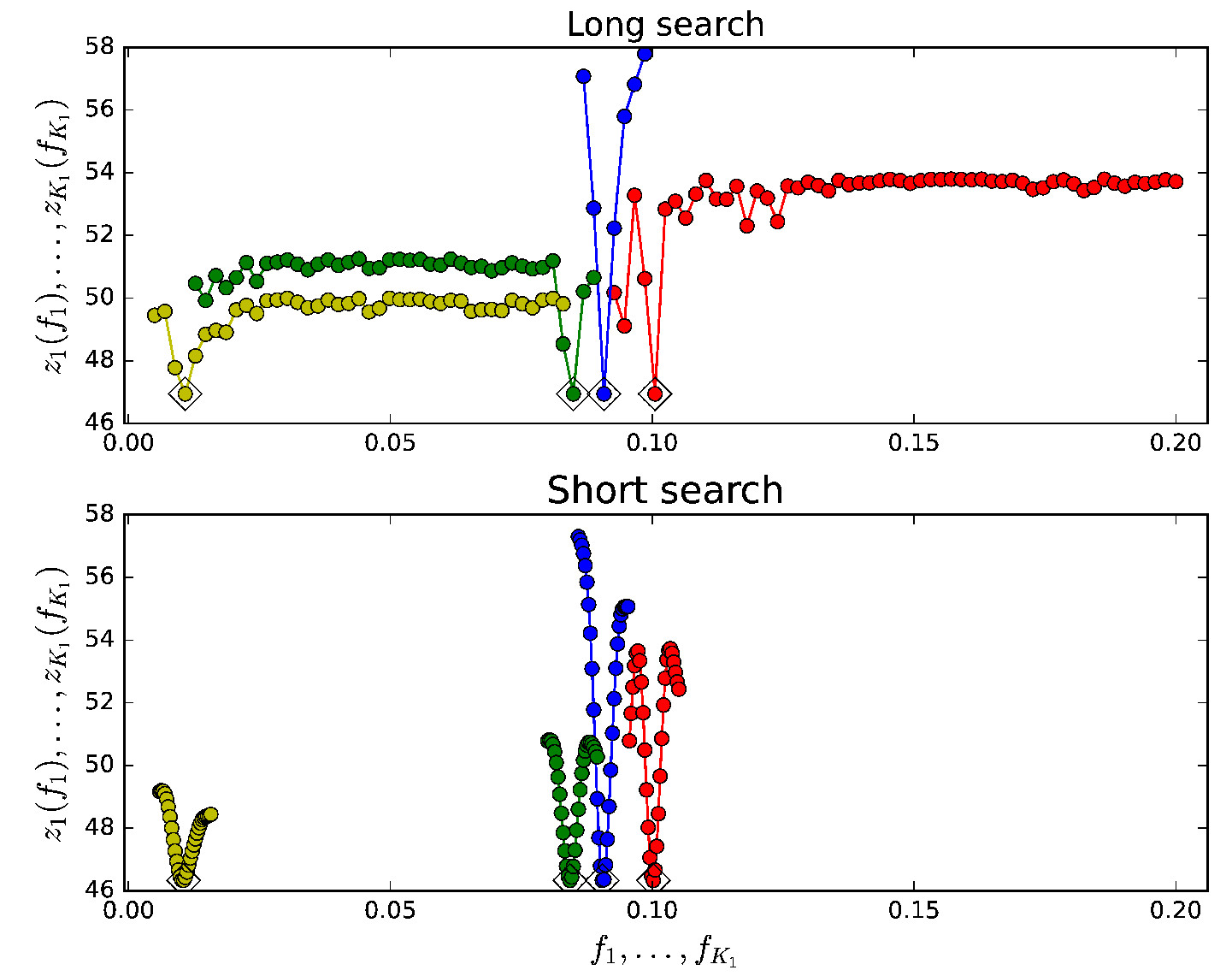
Figure 9: M=4 model in Table 12. Four pure sine signal periodograms for Rmonthly2000 between $P_{\mathrm{min}}=5$ and $P_{\mathrm{max}}=200$ years. We test frequency grids having $n_{\mathrm{L}}=100$ and $n_{\mathrm{S}}=30$ tested frequencies. Upper panel shows long search $z_{1}(f_{1})$ (red) $z_{2}(f_{2})$ (blue) $z_{3}(f_{3})$ (green) and $z_{4}(f_{4})$ (yellow) periodograms (Eq. B17) for a $n_{\mathrm{L}}=80$ frequency grid. Best frequencies are marked with diamonds. Units are x-axis $[f]=$ 1/years and y-axis $[z]=$ dimensionless. Lower panel shows short search periodograms for a denser $n_{\mathrm{S}}=30$ frequency grid having an interval width $c=0.05\equiv$ 5% (Eq. B16). Otherwise as in upper panel.

We search for periods between $P_{\mathrm{min}}=1/f_{\mathrm{max}}=5$ years and $P_{\mathrm{max}}=1/f_{\mathrm{min}}=200$ years.

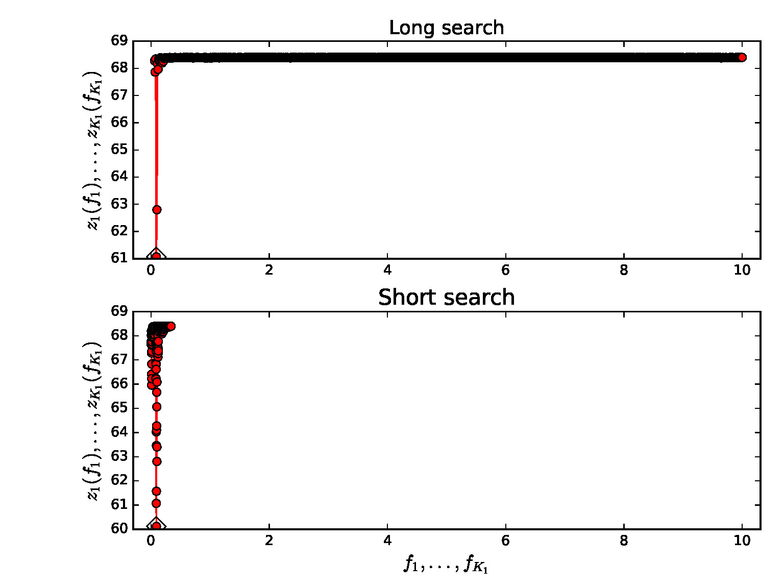
Figure 10: One pure sine signal $z_{1}(f_{1})$ periodogram for Rmonthly2000 between $P_{\mathrm{min}}=0.01$ and $P_{\mathrm{max}}=20$ years. We test “overkill” dense frequency grids $n_{L}=1000$ and $n_{S}=500$ to search for short frequencies, but detect none. Best period is $P_{1}=11.034$ years, which also given Table 10 ($\mathcal{M}$=1).

The global periodogram minimum

$$z_{\mathrm{min}}=z(f_{\mathrm{1,best}},f_{\mathrm{2,best}},...,f_{\mathrm{K_{1},best}}),$$

is at the tested frequencies $f_{\mathrm{1,best}},f_{\mathrm{2,best}},...,f_{\mathrm{K_{1},best}}$. The best model for the data has these signal frequencies.

The scalar $z$ periodogram values are computed from $K_{1}$ frequency values. For example, $K_{1}=2$ two signal periodogram $z(f_{1},f_{2})$ could be plotted like a map, where $f_{1}$ and $f_{2}$ are the coordinates, and $z=z(f_{1},f_{2})$ is the height. For three or more signals, such direct graphical presentation becomes impossible, because it requires more than three dimensions. We solve this problem by presenting only the following one-dimensional slices of the full periodogram

$$z_{1}(f_{1}) = z(f_{1},f_{\mathrm{2,best}},...,f_{\mathrm{K_{1},best}})$$

$$z_{2}(f_{2}) = z(f_{\mathrm{1,best}},f_{2},f_{\mathrm{3,best}},...,f_{\mathrm{K_{1},best}})$$

$$z_{3}(f_{3}) = z(f_{\mathrm{1,best}},f_{\mathrm{2,best}},f_{3},f_{\mathrm{4,best}},...,f_{\mathrm{K_{1},best}})~{}$$

$$z_{4}(f_{4}) = z(f_{\mathrm{1,best}},f_{\mathrm{2,best}},f_{\mathrm{3,best}},f_{4},f_{\mathrm{5,best}},f_{\mathrm{K_{1},best}})$$ (B17)

$$z_{5}(f_{5}) = z(f_{\mathrm{1,best}},f_{\mathrm{2,best}},f_{\mathrm{3,best}},f_{\mathrm{4,best}},f_{5},f_{\mathrm{K_{1},best}})$$

$$z_{6}(f_{6}) = z(f_{\mathrm{1,best}},f_{\mathrm{2,best}},f_{\mathrm{3,best}},f_{\mathrm{4,best}},f_{\mathrm{5,best}},f_{6}).$$

Using the above $K_{1}=2$ map analogy, the slice $z_{1}(f_{1})$ represents the height $z$ at $f_{1}$ coordinate when moving along the constant line $f_{2}=f_{\mathrm{2,best}}$ that crosses the global minimum $z_{\mathrm{min}}$.

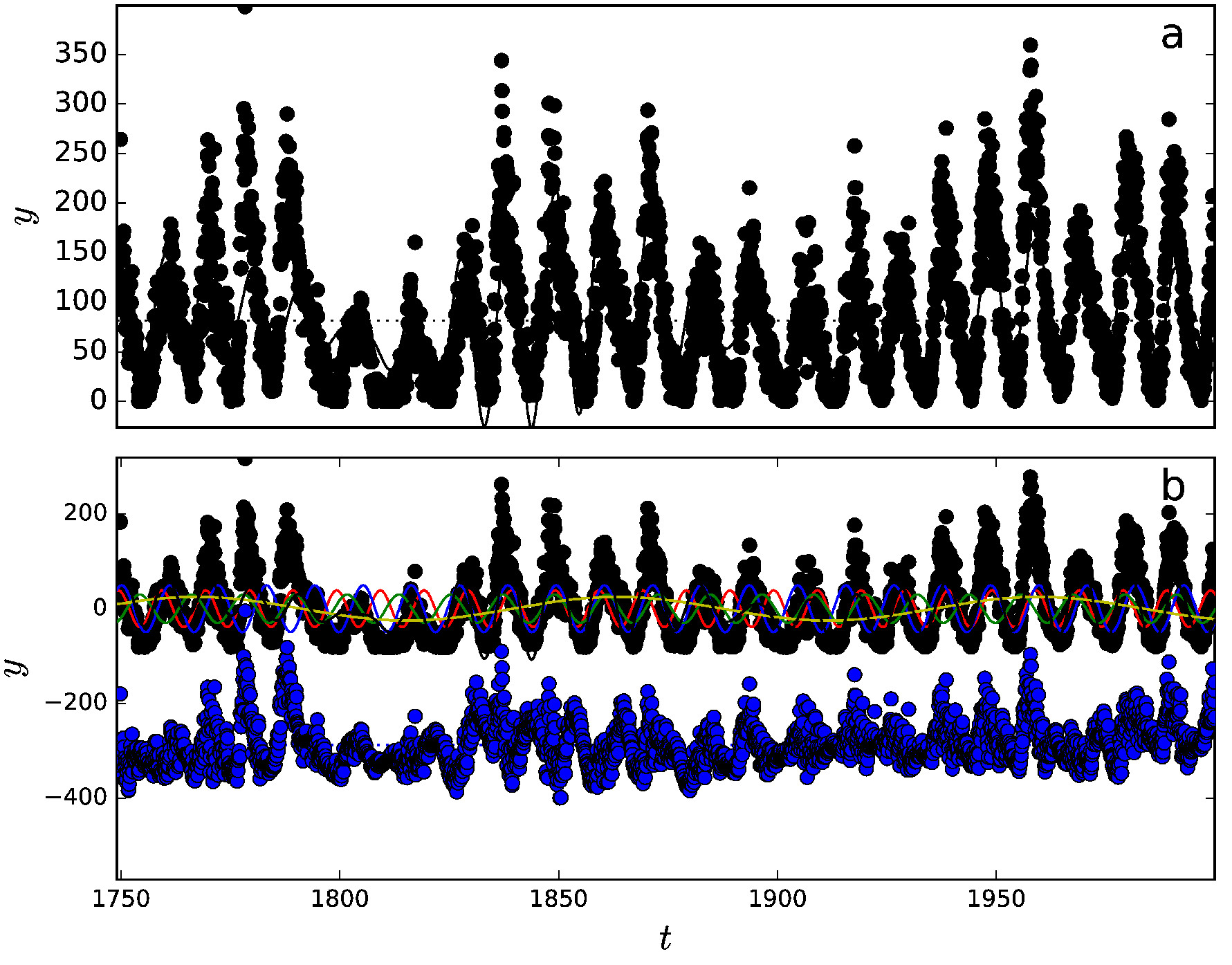
Figure 11: $\mathcal{M}$=4 model in Table 12. Upper panel shows data $y_{i}$ (black circles), $g(t)$ (continuous black curve) and constant trend $p(t)$ (dotted black curve). Units are x-axis $[t]=$ years and y-axis $[y]=$ dimensionless. Lower panel shows data minus $p(t)$ values (black circles), and $g(t)-p(t)$ (black curve), $h_{1}(t)$ (red curve), $h_{2}(t)$ (blue curve), $h_{3}(t)$ (green curve) and $h_{4}(t)$ (yellow curve). Residuals (blue circles) are offset to $y=-300$ level. Signal periods are $P_{1}=9.9842$, $P_{2}=11.0234$, $P_{3}=11.846$ and $P_{4}=96.2$ years.

The best frequencies detected in the short search give the initial values for free parameters $\bar{\beta}_{\mathrm{I,initial}}$ (Eq. B11). The linear model with these frequencies gives initial values for $\bar{\beta}_{\mathrm{II,initial}}$ (Eq. B12). The final non-linear iteration is performed from

$$\bar{\beta}_{\mathrm{initial}}=[\bar{\beta}_{\mathrm{I,initial}},\bar{\beta}_{\mathrm{II,initial}}]\rightarrow\bar{\beta}_{\mathrm{final}}$$ (B18)

The Rmonthly2000 sample four pure sine signal model periodograms between $P_{\mathrm{min}}=5$ and $P_{\mathrm{max}}=200$ years are shown in Fig. 9 (Table 10: $\mathcal{M}$=4 model). The one pure sine signal  periodogram for the same Rmonthly2000 sample between $P_{\mathrm{min}}=0.01$ and $P_{\mathrm{max}}=20$ years shows no signs of short periods (Fig. 10). The four pure sine signal $g(t)$ model for Rmonthly2000 is shown in Fig. 11.

DCM determines the following parameters for $h_{i}(t)$ signals

• $P_{i}=1/f_{i}=$ Period

• $A_{i}=$ Peak to peak amplitude

• $t_{\mathrm{i,min,1}}=$ Deeper primary minimum epoch

• $t_{\mathrm{i,min,2}}=$ Secondary minimum epoch (if present)

• $t_{\mathrm{i,max,1}}=$ Higher primary maximum epoch

• $t_{\mathrm{i,max,2}}=$ Secondary maximum epoch (if present),

as well the $M_{k}$ parameters of the $p(t)$ trend. For the sunspots, the most interesting parameters are the signal periods $P_{i}$, the signal amplitudes $A_{i}$, and signal primary minimum epochs $t_{\mathrm{min,1}}$ (Tables 10-21).

Each $h_{j}(t)$ signal

$$y_{i,j}=y_{i}-[g(t_{i})-h_{j}(t_{i})]$$ (B19)

of model $\mathcal{M}$=4 in Table 10 is shown separately in Fig. 12.

The DCM model parameter errors are determined with the bootstrap procedure (Efron & Tibshirani, 1986). We have previously used this same bootstrap procedure in our TSPA- and CPS-methods (Jetsu & Pelt, 1999; Lehtinen et al., 2011). A random sample $\bar{\epsilon}^{*}$ is selected from the residuals $\bar{\epsilon}$ of the DCM model (Eq. B6). Any $\epsilon_{i}$ can be chosen as many times as the random selection happens to favour it. This random sample of residuals gives the artificial bootstrap data sample

$$y_{i}^{*}=g_{i}+\epsilon_{i}^{*}.$$ (B20)

We create numerous such $\bar{y}^{*}$ random samples. DCM model for each $\bar{y}^{*}$ sample gives one estimate for every model parameter. The error estimate for each particular model parameter is the standard deviation of all estimates obtained from all $\bar{y}^{*}$ bootstrap samples.

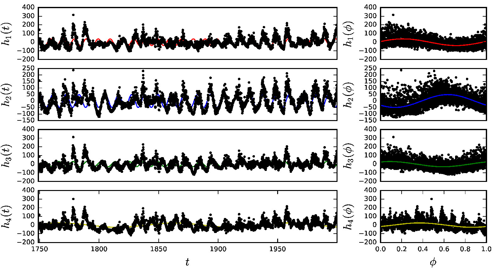
Figure 12: $\mathcal{M}$=4 model in Table 12. Left panels show four signals $g_{i,j}$ (Eq. B19) as a function of time. Units are x-axis $[t]=$ years and y-axis $[h_{i}(t)]=$ dimensionless. Right panels show same signals as function of phase. Units are x-axis $[\phi]=$ dimensions and y-axis $[h_{i}(t)]=$ dimensionless. Signal periods are $P_{1}=9.9842$, $P_{2}=11.0234$, $P_{3}=11.846$ and $P_{4}=96.2$ years. Curve colours are as in Fig. 11.

Figure 13: Extracts: (a) Rmonthly2000 double sinusoid $23.686\pm 0.018$ year signal is exactly equal to two times Jupiter’s 11.86 year period. (b) Rmonthly double sinusoid $20.0062\pm 0.0082$ year signal is exactly equal to two times 10 years. Numbers and labels for x-axis phases $\phi$ between 0 and 1 are missing, because these figures are extracts from larger figures, like Fig. 12. Units are x-axis $[\phi]=$ dimensionless and y-axis $[y]=$ dimensionless.

DCM models are nested. For example, a one signal model is a special case of a two signal model. As for another example, $\mathcal{M}$=2 model is more complex than $\mathcal{M}$=1 model in Table 10. DCM uses the Fisher-test to compare any pair of simple $g_{1}(t)$ and complex $g_{2}(t)$ models. Their number of free parameters are $\eta_{1}<\eta_{2}$. Their sums of squared residuals $(R_{1},R_{2})$ and Chi-squares $(\chi_{1},\chi_{2})$ give the Fisher-test test statistic

$$F_{R} = \left({{R_{1}}\over{R_{2}}}-1\right)\left({{n-\eta_{2}-1}\over{\eta_{2}-\eta_{1}}}\right).$$ (B21)

$$F_{\chi} = \left({{\chi_{1}^{2}}\over{\chi_{2}^{2}}}-1\right)\left({{n-\eta_{2}-1}\over{\eta_{2}-\eta_{1}}}\right).$$ (B22)

The Fisher-test null hypothesis is

• $H_{\mathrm{0}}$: “The complex model $g_{2}(t)$ does not provide a significantly better fit to the data than the simple model $g_{\mathrm{1}}(t)$.”

Under $H_{0}$, both test statistic parameters $F_{R}$ and $F_{\chi}$ have an $F$ distribution with $(\nu_{1},\nu_{2})$ degrees of freedom, where $\nu_{1}=\eta_{2}-\eta_{1}$ and $\nu_{2}=n-\eta_{2}$ (Draper & Smith, 1998). The probability for $F_{R}$ or $F_{\chi}$ reaching values higher than $F$ is called the critical level $Q_{F}=P(F_{R}\geq F)$ or $Q_{F}=P(F_{\chi}\geq F)$. We reject the $H_{0}$ hypothesis, if

$$Q_{F}<\gamma_{F}=0.001,$$ (B23)

where $\gamma_{F}$ is the pre-assigned significance level. This $\gamma_{F}$ represents the probability of falsely rejecting $H_{0}$ hypothesis when it is in fact true. If $H_{0}$ is rejected, we rate the complex $g_{2}(t)$ model better than the simple $g_{1}(t)$ model.

The basic idea of the Fisher-test is simple. The $H_{0}$ hypothesis rejection probability increases for larger $F_{R}$ values having smaller $Q_{F}$ critical level. The complex model $R_{2}$ or $\chi^{2}_{2}$ values decrease when the $\eta_{2}$ number of free parameters increases. This increases the first $(R_{1}/R_{2}-1)$ and $(\chi^{2}_{1}/\chi^{2}_{2}-1)$ terms in Eqs. B21 and B22. However, the second $(n-\eta_{2}-1)/(\eta_{2}-\eta_{1})$ penalty term decreases at the same time. This second penalty term prevents over-fitting, i.e. accepting complex models having too many $\eta_{2}$ free parameters.

DCM model can be used to predict future and past data. The samples in these predictions are

• Predictive data sample: $t_{i}$, $y_{i}$ and $\sigma_{i}$ contains $n$ values

• Predicted data sample: $t_{i}^{\prime}$, $y_{i}^{\prime}$ and $\sigma_{i}^{\prime}$ contains $n^{\prime}$ values

• Combined predictive and predicted data sample: $t^{\prime\prime}_{i}$, $y^{\prime\prime}_{i}$ and $\sigma^{\prime\prime}_{i}$ contains $n^{\prime\prime}=n+n^{\prime}$ values

We compute the $t_{\mathrm{mid}}$ and $\Delta T$ values from the time points $t_{i}$ of the predictive data. DCM gives the best model $g(t,\bar{\beta})$ for the predictive data. The “old” predictive data $t_{\mathrm{mid}}$ and $\Delta T$ values are used to compute the predicted and combined data models

$$g^{\prime}(t^{\prime}) = g^{\prime}(t,^{\prime}\bar{\beta})$$

$$g^{\prime\prime}(t^{\prime\prime}) = g^{\prime\prime}(t^{\prime\prime},\bar{\beta}).$$

In other words, we do not compute “new” $t_{\mathrm{mid}}$ and $\Delta T$ values from the time points $t^{\prime}_{i}$ or $t^{\prime\prime}_{i}$. There is an obvious reason for this. The predictive data free parameter values $\bar{\beta}$ give the correct $g^{\prime}(t,^{\prime}\bar{\beta})$ and $g^{\prime\prime}(t^{\prime\prime},\bar{\beta})$ values only for the “old” predictive data $t_{\mathrm{mid}}$ and $\Delta T$ values.

The residuals

$$\epsilon^{\prime}_{i}=y^{\prime}_{i}-g^{\prime}_{i}$$

give

$$z^{\prime}=\textnormal{Predicted data test statistic (Eq. \ref{EqzR} and \ref{EqzChi})}$$ (B24)

We emphasize that the predictive data $t_{\mathrm{mid}}$ and $\Delta T$ values can be used to compute the model value for any arbitrary $t^{\prime}_{i}$ time point values. This gives parameters, like the value

$$g^{\prime\prime}_{\mathrm{mean}}={{1}\over{n^{\prime\prime}}}\sum_{i=1}^{n^{\prime\prime}}g^{\prime\prime}(t^{\prime\prime}_{i},\bar{\beta}).$$ (B25)

of the combined data model mean for any arbitrary time points $t^{\prime\prime}_{i}$.

Figure 14: $\mathcal{M}$=4 model in Table 12. Left hand panels show bootstrap signal frequency estimates $(f_{1},f_{2},f_{3},f_{4})$. Units are $[f_{i}]=$ 1/years. Right hand panels show respective amplitude estimates $(A_{1},A_{2},A_{3},A_{4})$. Units are $[A_{i}]=$ dimensionless. Larger blue circles denote values for original data. Smaller red circles denote values for bootstrap random samples. Dotted lines denote one, two and three sigma error limits.

The key ideas of DCM are based on the following robust thoroughly tested statistical approaches

1. DCM model $g(t)$ is non-linear (Eq. B1). This model becomes linear when the frequencies $f_{1},...,f_{K_{1}}$ are fixed to their tested numerical values. This linear model gives unambiguous results.

2. DCM tests a dense grid of all possible frequency combinations $f_{\mathrm{min}}\leq f_{1}\!>\!f_{2}\!>\!...\!>\!f_{K_{1}}\leq f_{\mathrm{max}}$ (Eq. B15). For every frequency combination, the linear model least squares fit gives the test statistic $z=\sqrt{\chi^{2}/n}$ (errors $\sigma_{i}$ known) or $z=\sqrt{R/n}$ (errors $\sigma_{i}$ unknown).

3. The short search $f_{\mathrm{1,best}}>f_{\mathrm{1,best}}>...>f_{\mathrm{K_{1},best}}$ grid combination that minimizes the $z$ test statistic gives the best initial $\bar{\beta}_{\mathrm{initial}}$ values for the non-linear iteration of Eq. B18.

4. The error estimates for all model parameters are determined with the bootstrap method (Eq. B20).

5. The best model is identified using the Fisher-test, which compares all different $K_{1}$, $K_{2}$ and $K_{3}$ order nested models (Draper & Smith, 1998; Allen, 2004).

DCM has the following restrictions

1. An adequately dense tested frequency grid eliminates the possibility that the best frequency combination is missed. The restriction is that denser grids require more computation time. For example, all four signal $z_{1}$, $z_{2}$, $z_{3}$ and $z_{4}$ periodograms for Rmonthly2000 data are continuous in Fig. 9. No abrupt periodogram jumps occur, because the $z$ values for all close tested frequencies correlate. The frequencies of the minima of all these periodograms are accurately determined. There is no need to test an even denser grid, because this would not alter the final result of the non-linear iteration of Eq. B18.

2. If the long search grid of each tested $f_{1}>f_{2}>...>f_{K_{1}}$ frequencies uses a value $n_{L}$, the total number of tested frequencies is

   $$\binom{n_{L}}{K_{1}}={{n_{L}!}\over{K_{1}!(n_{L}-K_{1})!}}$$

   For example, it took 3 days wall-clock time, and over 300 days of cpu-time, for a cluster of computers to compute the five signal DCM model shown in Fig. 15.

3. Some DCM models are unstable. They are simply wrong models for the data, like a wrong $p(t)$ trend order $K_{3}$, or a search for too few or too many $K_{1}$ signals (e.g. Paper I: Figs. 5-10). This causes model instability. We denote such unstable models with “${\color[rgb]{0,0,1}{\bf\mathrm{UM}}}$” in Tables 10-21. The signatures of such unstable models are

   • “${\color[rgb]{0,0,1}{\bf\mathrm{IF}}}$” = Intersecting frequencies

   • “${\color[rgb]{0,0,1}{\bf\mathrm{AD}}}$” = Dispersing amplitudes

   • “${\color[rgb]{0,0,1}{\bf\mathrm{LP}}}$” = Leaking periods

4. Intersecting frequencies “${\color[rgb]{0,0,1}{\bf\mathrm{IF}}}$” occur when the frequencies of two signals are very close to each other. For example, if frequency $f_{1}$ approaches frequency $f_{2}$, the $h_{1}(t)$ and $h_{2}(t)$ signals become essentially one and the same signal. This ruins the least squares fit. It makes no sense to add the same signal twice.

5. Dispersing amplitudes “${\color[rgb]{0,0,1}{\bf\mathrm{AD}}}$” also occur when two signal frequencies are close to each other, like in the “${\color[rgb]{0,0,1}{\bf\mathrm{IF}}}$” cases. The least squares fit uses two high amplitude signals which cancel out. Hence, the sum of these two high amplitude signals is one low amplitude signal that fits to the data.

6. We take extra care of the suspected “${\color[rgb]{0,0,1}{\bf\mathrm{IF}}}$” and $"{\color[rgb]{0,0,1}{\bf\mathrm{AD}}}$” cases. The reshuffling of bootstrap $\bar{\epsilon}^{\star}$ residuals is a good test for identifying such cases. If we encounter any signs of instability, we test combinations $n_{\mathrm{L}}=100~{}\&~{}c=0.05$, $n_{\mathrm{L}}=100~{}\&~{}c=0.10$, $n_{\mathrm{L}}=120~{}\&~{}c=0.05$ and $n_{\mathrm{L}}=120~{}\&~{}c=0.10$. If there is instability in any of these combinations, we reject the model as unstable $("{\color[rgb]{0,0,1}{\bf\mathrm{UM}}}")$. If there is no instability, we take the $n_{\mathrm{L}}$ and $c$ combination that gives the lowest value for $R$ (non-weighted data) or $\chi^{2}$ (weighted data).

7. Leaking periods “${\color[rgb]{0,0,1}{\bf\mathrm{LP}}}$” refer to the cases when the period $P=1/f$ given by the detected frequency $f$ is longer than the time span $\Delta T$ of the data.

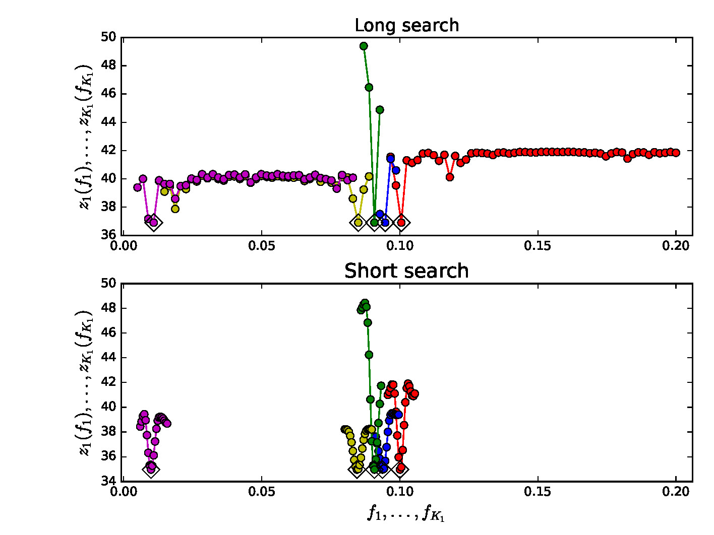
Figure 15: ”Buying all lottery tickets”. We compute pure five sine signal model periodograms for Ryearly $(n=322)$. Long search for $n_{\mathrm{L}}=100$ frequency grid requires testing of 79 208 745 models. Short $n_{\mathrm{S}}=20$ frequency grid requires testing of 2 451 267 models. Detected signals are 9.977, 10.637, 11.032, 11.815 and 101.339 years. Total consumed cpu-time exceeds 300 days. Note that error estimates are missing, because 20 bootstrap samples would require testing of $20\times 2~{}451~{}267$ additional models. Otherwise as in Fig. 9.

We conclude that DCM can test all reasonable alternative non-linear $g(t)$ models for the data. DCM determines the unambiguous results for the best values of the free parameters of all these alternative $g(t)$ models. DCM uses a brute numerical approach to find the best $g(t)$ model among all alternative models. DCM “works like winning a lottery by buying all lottery tickets” ( Paper I). The caption text of Fig. 15 elucidates how such lotteries are won in practice. In real life, it would make no sense win less money by investing more money to all lottery tickets. In science, investing enough computing time to DCM gives the correct answer for free.

B.1 DCM improvements

B.1.1 Parallel computation

We began the sunspot data analysis in December 2022, and soon discovered the exact 10 and 11 year periods, as well as the 11.86 period, in the yearly data. Then we realized that this discovery could be disputed by arguing that the one year data window produces such spurious periods. We decided to bypass this problem by analysing the monthly sunspot data. However, the much larger size of these samples slowed down our analysis. The logical solution was to develop a parallel DCM computation code.

In the appendix of Paper I, we gave detailed instructions for using the DCM python code. That “manual” is adequate for repeating the analysis in this paper. Here, we provide all necessary information for reproducing our current DCM analysis of sunspot data. The 24 first control file dcm.dat parameters are the same as in Paper I and Paper II.

We have added the following three new parameters into the control file dcm.dat.

• Parallel=1 activates the “new” parallel computation mode. Parallel$\neq$ 1 activates the “old” serial computation mode.

• PoolNumber defines the number of simultaneous processes in parallel computation.

• ChunkModels chops the long tested frequency vectors into shorter pieces. In this way, we can bypass the problem that python slows down when vectors become very long.

B.1.2 No trend

The “ new” control parameter value K3 $=K_{3}=-1$ means that the model has no polynomial part, i.e. $p(t)=0$. This alternative is useful in the residual analysis, where all trends have already been removed. The “old” alternative K3$=K_{3}=0$ would still remove a constant level trend $p(t)=M_{0}$, and this could mislead the analysis.

Table 10: Rmonthly2000 analysis for pure sines $(K_{2}=1)$. We use first model $\mathcal{M}$=1 as an example of how to read this table. (1) Model number $\mathcal{M}$=1. (2) Chosen $\mathcal{M}$${}_{K_{1}=1,K_{2}=1,K_{3}=0,R}$ model has $\eta=4$ free parameters, and its sum of squared residuals is $R=1.09\times 10^{7}$. (3) First signal period is $P_{1}=11.0336\pm 0.0074$ years. Dimensionless peak to peak amplitude is $A_{1}=92.2\pm 2.8$. Primary minimum epoch is at year $t_{\mathrm{min,1}}=1755.30\pm 0.12$. (4-6) Periods, amplitudes and primary minima for two, three and four signal models. (7) Every new model is more complex when going down this table because number $\eta$ of free parameters increases (Eq. B10). Fisher-test between simple $\mathcal{M}$=1 model and complex $\mathcal{M}$=2 model gives test statistic $F_{R}=255$ (Eq. B21) reaching a critical level $Q_{F}<10^{-16}$. Criterion $Q_{F}<\gamma=0.001$ is fulfilled (Eq. B23). Therefore, an upward arrow $\uparrow$ indicates that $\mathcal{M}$=2 model is a better model than $\mathcal{M}$=1 model. A leftward arrow $\leftarrow$ would have been used, if model $\mathcal{M}$=1 were better. (8-9) Fisher-tests for models $\mathcal{M}$=3 and 4. (10) Electronic control file Rmonthly2000K110R14.dat can be used to repeat whole DCM analysis of $\mathcal{M}$=1. Four first signals are detected from original data in electronic file Rmontly2000.dat. Next four model $\mathcal{M}$=5-8 signals are detected from residuals of model $\mathcal{M}$=4, which are stored to electronic file RmonthlyK410R14Residuals.dat. Models $\mathcal{M}$=7 and 8 are unstable $({\color[rgb]{0,0,1}{\bf\mathrm{UM}}})$ because they suffer from amplitude dispersion $({\color[rgb]{0,0,1}{\bf\mathrm{AD}}})$. Intersecting frequencies $({\color[rgb]{0,0,1}{\bf\mathrm{IF}}})$ or leaking periods $({\color[rgb]{0,0,1}{\bf\mathrm{LP}}})$ are not encountered in any of these eight $\mathcal{M}$=1-8 models. Models $\mathcal{M}$=4 and 6 give final results summarized in Table 2.

		Period analysis					Fisher-test
Data: Original non-weighted data ($n=3012,\Delta T=250.9$: Rmonthly2000.dat)
$\mathcal{M}$	$\mathcal{M}$${}_{K_{1},K_{2},K_{3},R}$	$P_{1}$ (y)	$P_{2}$ (y)	$P_{3}$ (y)	$P_{4}$ (y)		$\mathcal{M}$=2	$\mathcal{M}$=3	$\mathcal{M}$=4
	$\eta$ (-)	$A_{1}$ (-)	$A_{2}$ (-)	$A_{3}$ (-)	$A_{4}$ (-)		$F_{R}$ (-)	$F_{R}$ (-)	$F_{R}$ (-)	Control file
	$R$ (-)	$t_{\mathrm{min,1}}$ (y)	$t_{\mathrm{min,1}}$ (y)	$t_{\mathrm{min,1}}$ (y)	$t_{\mathrm{min,1}}$ (y)		$Q_{F}$ (-)	$Q_{F}$ (-)	$Q_{F}$ (-)
(1)	(2)	(3)	(4)	(5)	(6)		(7)	(8)	(9)	(10)
$\mathcal{M}$=1	$\mathcal{M}$1,1,0,R	$11.0336\!\!\pm\!\!0.0074$	-	-	-		$\uparrow$	$\uparrow$	$\uparrow$
	4	$92.2\!\!\pm\!\!2.8$	-	-	-		255	254	231	Rmonthly2000K110R14.dat
	$1.09\!\!\times\!\!10^{7}$	$1755.30\!\!\pm\!\!0.12$	-	-	-		$<\!10^{-16}$	$<\!10^{-16}$	$<\!10^{-16}$
$\mathcal{M}$=2	$\mathcal{M}$2,1,0,R	$9.9998\!\!\pm\!\!0.0060$	$11.0200\!\!\pm\!\!0.0074$	-	-		-	$\uparrow$	$\uparrow$
	7	$76.7\!\!\pm\!\!2.5$	$91.6\!\!\pm\!\!3.2$	-	-		-	179	174	Rmonthly2000K210R14.dat
	$8.69\!\!\times\!\!10^{6}$	$1754.18\!\!\pm\!\!0.11$	$1755.65\!\!\pm\!\!0.11$	-	-		-	$<\!10^{-16}$	$<\!10^{-16}$
$\mathcal{M}$=3	$\mathcal{M}$3,1,0,R	$9.9848\!\!\pm\!\!0.0076$	$11.0293\!\!\pm\!\!0.0065$	$11.845\!\!\pm\!\!0.012$	-		-	-	$\uparrow$
	10	$77.0\!\!\pm\!\!2.4$	$99.6\!\!\pm\!\!2.9$	$60.8\!\!\pm\!\!1.8$	-		-	-	144	Rmonthly2000K310R14.dat
	$7.37\!\!\times\!\!10^{6}$	$1754.36\!\!\pm\!\!0.12$	$1755.704\!\!\pm\!\!0.089$	$1760.24\!\!\pm\!\!0.16$	-		-	-	$<\!10^{-16}$
$\mathcal{M}$=4	$\mathcal{M}$4,1,0,R	$9.9842\!\!\pm\!\!0.0075$	$11.0324\!\!\pm\!\!0.0048$	$11.846\!\!\pm\!\!0.012$	$96.2\!\!\pm\!\!1.0$		-	-	-
	13	$77.4\!\!\pm\!\!2.2$	$98.8\!\!\pm\!\!2.6$	$60.0\!\!\pm\!\!2.2$	$50.1\!\!\pm\!\!2.8$		-	-	-	Rmonthly2000K410R14.dat
	$6.44\!\!\times\!\!10^{6}$	$1754.363\!\!\pm\!\!0.096$	$1755.661\!\!\pm\!\!0.075$	$1760.22\!\!\pm\!\!0.16$	$1815.3\!\!\pm\!\!1.0$		-	-	-
Data: Non-weighted residuals of model $\mathcal{M}$=4 ($n=3012,\Delta T=250.9$: Rmonthly2000K410R14Residuals.dat)
							$\mathcal{M}$=6	$\mathcal{M}$=7	$\mathcal{M}$=8
$\mathcal{M}$=5	$\mathcal{M}$1,1,-1,R	$10.547\!\!\pm\!\!0.012$	-	-	-		$\uparrow$	$\uparrow$	$\uparrow$
	3	$45.3\!\!\pm\!\!1.8$	-	-	-		97	92	96	Rmonthly2000K11-1R58.dat
	$5.67\!\!\times\!\!10^{6}$	$1753.04\!\!\pm\!\!0.16$	-	-	-		$<\!10^{-16}$	$<\!10^{-16}$	$<\!10^{-16}$
$\mathcal{M}$=6	$\mathcal{M}$2,1,-1,R	$8.1054\!\!\pm\!\!0.0084$	$10.541\!\!\pm\!\!0.014$	-	-		-	$\uparrow$	$\uparrow$
	6	$36.5\!\!\pm\!\!1.7$	$45.0\!\!\pm\!\!1.8$	-	-		-	79	87	Rmonthly2000K21-1R58.dat
	$5.17\!\!\times\!\!10^{6}$	$1751.33\!\!\pm\!\!0.13$	$1753.13\!\!\pm\!\!0.20$	-	-		-	$<\!10^{-16}$	$<\!10^{-16}$
$\mathcal{M}$=7	$\mathcal{M}$3,1,-1,R	$8.174\!\!\pm\!\!0.033$	$8.381\!\!\pm\!\!0.029$	$105.409\!\!\pm\!\!0.010$	-		-	-	$\uparrow$
${\color[rgb]{0,0,1}{\bf\mathrm{UM}}}$	9	$40\!\!\pm\!\!57~{}{\color[rgb]{0,0,1}{\bf\mathrm{AD}}}$	$40\!\!\pm\!\!57~{}{\color[rgb]{0,0,1}{\bf\mathrm{AD}}}$	$45.6\!\!\pm\!\!1.4$	-		-	-	89	Rmonthly2000K31-1R58.dat
	$4.79\!\!\times\!\!10^{6}$	$1750.23\!\!\pm\!\!0.58$	$1750.67\!\!\pm\!\!0.53$	$1753.13\!\!\pm\!\!0.13$	-		-	-	$<\!10^{-16}$
$\mathcal{M}$=8	$\mathcal{M}$4,1,-1,R	$8.175\!\!\pm\!\!0.026$	$8.384\!\!\pm\!\!0.032$	$10.543\!\!\pm\!\!0.010$	$52.08\!\!\pm\!\!0.36$		-	-	-
${\color[rgb]{0,0,1}{\bf\mathrm{UM}}}$	12	$39\!\!\pm\!\!25~{}{\color[rgb]{0,0,1}{\bf\mathrm{AD}}}$	$39\!\!\pm\!\!24~{}{\color[rgb]{0,0,1}{\bf\mathrm{AD}}}$	$45.7\!\!\pm\!\!2.1$	$31.6\!\!\pm\!\!2.1$		-	-	-	Rmonthly2000K41-1R58.dat
	$4.40\!\!\times\!\!10^{6}$	$1750.22\!\!\pm\!\!0.52$	$1750.64\!\!\pm\!\!0.39$	$1753.11\!\!\pm\!\!0.13$	$1760.2\!\!\pm\!\!1.0$		-	-	-

Table 11: Rmonthly2000 analysis for double waves $(K_{2}=2)$. Otherwise as in Table 10.

		Period analysis					Fisher-test
Data: Non-weighted original data ($n=3012,\Delta T=250.9$: Rmonthly2000.dat)
$\mathcal{M}$	$\mathcal{M}$${}_{K_{1},K_{2},K_{3},R}$	$P_{1}$ (y)	$P_{2}$ (y)	$P_{3}$ (y)	$P_{4}$ (y)		$\mathcal{M}$=2	$\mathcal{M}$=3	$\mathcal{M}$=4
	$\eta$ (-)	$A_{1}$ (-)	$A_{2}$ (-)	$A_{3}$ (-)	$A_{4}$ (-)		$F_{R}$ (-)	$F_{R}$ (-)	$F_{R}$ (-)	Control file
	$R$ (-)	$t_{\mathrm{min,1}}$ (y)	$t_{\mathrm{min,1}}$ (y)	$t_{\mathrm{min,1}}$ (y)	$t_{\mathrm{min,1}}$ (y)		$Q_{F}$ (-)	$Q_{F}$ (-)	$Q_{F}$ (-)
(1)	(2)	(3)	(4)	(5)	(6)		(7)	(8)	(9)	(10)
$\mathcal{M}$=1	$\mathcal{M}$1,2,0,R	$11.0242\!\!\pm\!\!0.0084$	-	-	-		$\uparrow$	$\uparrow$	$\uparrow$
	6	$94.7\!\!\pm\!\!3.6$	-	-	-		154	149	164	Rmonthly2000K120R14.dat
	$1.08\!\!\times\!\!10^{7}$	$1755.98\!\!\pm\!\!0.12$	-	-	-		$<\!10^{-16}$	$<\!10^{-16}$	$<\!10^{-16}$
$\mathcal{M}$=2	$\mathcal{M}$2,2,0,R	$11.0118\!\!\pm\!\!0.0071$	$20.000\!\!\pm\!\!0.016$	-	-		-	$\uparrow$	$\uparrow$
	11	$95.0\!\!\pm\!\!2.8$	$81.2\!\!\pm\!\!2.4$	-	-		-	115	135	Rmonthly2000K220R14.dat
	$8.59\!\!\times\!\!10^{6}$	$1756.33\!\!\pm\!\!0.15$	$1764.12\!\!\pm\!\!0.11$	-	-		-	$<\!10^{-16}$	$<\!10^{-16}$
$\mathcal{M}$=3	$\mathcal{M}$3,2,0,R	$9.9862\!\!\pm\!\!0.0068$	$11.0222\!\!\pm\!\!0.0062$	$23.692\!\!\pm\!\!0.021$	-		-	-	$\uparrow$
	16	$78.7\!\!\pm\!\!1.8$	$103.3\!\!\pm\!\!2.9$	$69.1\!\!\pm\!\!2.4$	-		-	-	130	Rmonthly2000K320R14.dat
	$7.21\!\!\times\!\!10^{6}$	$1754.72\!\!\pm\!\!0.18$	$1756.33\!\!\pm\!\!0.12$	$1760.11\!\!\pm\!\!0.13$	-		-	-	$<\!10^{-16}$
$\mathcal{M}$=4	$\mathcal{M}$4,2,0,R	$9.9882\!\!\pm\!\!0.0061$	$11.0234\!\!\pm\!\!0.0068$	$23.686\!\!\pm\!\!0.018$	$104.16\!\!\pm\!\!0.59$		-	-	-
	21	$78.6\!\!\pm\!\!2.6$	$102.9\!\!\pm\!\!2.7$	$69.4\!\!\pm\!\!2.7$	$70.4\!\!\pm\!\!3.6$		-	-	-	Rmonthly2000K420R148.dat
	$5.92\!\!\times\!\!10^{6}$	$1754.70\!\!\pm\!\!0.11$	$1756.295\!\!\pm\!\!0.099$	$1760.13\!\!\pm\!\!0.14$	$1811.43\!\!\pm\!\!0.54$		-	-	-
Data: Non-weighted residuals of $\mathcal{M}$=4 ($n=3012,\Delta T=250.9$: Rmonthly2000K420R14Residuals.dat)
							$\mathcal{M}$=6	$\mathcal{M}$=7	$\mathcal{M}$=8
$\mathcal{M}$=5	$\mathcal{M}$1,2,-1,R	$10.5400\!\!\pm\!\!0.0095$	-	-	-		$\uparrow$	$\uparrow$	$\uparrow$
	5	$51.1\!\!\pm\!\!2.6$	-	-	-		68	69	74	Rmonthly2000K12-1R58.dat
	$5.04\!\!\times\!\!10^{6}$	$1754.34\!\!\pm\!\!0.19$	-	-	-		$<\!10^{-16}$	$<\!10^{-16}$	$<\!10^{-16}$
$\mathcal{M}$=6	$\mathcal{M}$2,2,-1,R	$10.5386\!\!\pm\!\!0.0076$	$16.215\!\!\pm\!\!0.014$	-	-		-	$\uparrow$	$\uparrow$
	10	$51.5\!\!\pm\!\!2.6$	$41.6\!\!\pm\!\!3.0$	-	-		-	63	70	Rmonthly2000K22-1R58.dat
	$4.53\!\!\times\!\!10^{6}$	$1754.41\!\!\pm\!\!0.19$	$1751.20\!\!\pm\!\!0.16$	-	-		-	$<\!10^{-16}$	$<\!10^{-16}$
$\mathcal{M}$=7	$\mathcal{M}$3,2,-1,R	$8.177\!\!\pm\!\!0.010$	$10.5400\!\!\pm\!\!0.0071$	$16.764\!\!\pm\!\!0.033$	-		-	-	$\uparrow$
	15	$39.6\!\!\pm\!\!4.0$	$51.7\!\!\pm\!\!2.2$	$46.0\!\!\pm\!\!4.4$	-		-	-	70	Rmonthly2000K32-1R58.dat
	$4.10\!\!\times\!\!10^{6}$	$1750.46\!\!\pm\!\!0.60$	$1754.35\!\!\pm\!\!0.10$	$1759.23\!\!\pm\!\!0.26$	-		-	-	$<\!10^{-16}$
$\mathcal{M}$=8	$\mathcal{M}$4,2,-1,R	$8.173\!\!\pm\!\!0.011$	$10.5372\!\!\pm\!\!0.0075$	$16.781\!\!\pm\!\!0.034$	$136.43\!\!\pm\!\!0.99$		-	-	-
	20	$37.6\!\!\pm\!\!4.8$	$51.2\!\!\pm\!\!1.8$	$44.9\!\!\pm\!\!4.0$	$42.3\!\!\pm\!\!2.2$		-	-	-	Rmonthly2000K42-1R58.dat
	$3.67\!\!\times\!\!10^{6}$	$1750.76\!\!\pm\!\!0.64$	$1754.38\!\!\pm\!\!0.12$	$1759.13\!\!\pm\!\!0.25$	$1884.10\!\!\pm\!\!0.91$		-	-	-

Table 12: Rmonthly analysis for pure sines $(K_{2}=1)$. Otherwise as in Table 10.

Data: Non-weighted original data ($n=3287,\Delta T=273.8$: Rmonthly.dat)
		Period analysis					Fisher-test
$\mathcal{M}$	$\mathcal{M}$${}_{K_{1},K_{2},K_{3},R}$	$P_{1}$ (y)	$P_{2}$ (y)	$P_{3}$ (y)	$P_{4}$ (y)		$\mathcal{M}$=2	$\mathcal{M}$=3	$\mathcal{M}$=4
	$\eta$ (-)	$A_{1}$ (-)	$A_{2}$ (-)	$A_{3}$ (-)	$A_{4}$ (-)		$F_{R}$ (-)	$F_{R}$ (-)	$F_{R}$ (-)	Control file
	$R$ (-)	$t_{\mathrm{min,1}}$ (y)	$t_{\mathrm{min,1}}$ (y)	$t_{\mathrm{min,1}}$ (y)	$t_{\mathrm{min,1}}$ (y)		$Q_{F}$ (-)	$Q_{F}$ (-)	$Q_{F}$ (-)
(1)	(2)	(3)	(4)	(5)	(6)		(7)	(8)	(9)	(10)
$\mathcal{M}$=1	$\mathcal{M}$1,1,0,R	$11.0046\!\!\pm\!\!0.0076$	-	-	-		$\uparrow$	$\uparrow$	$\uparrow$
	4	$93.8\!\!\pm\!\!2.3$	-	-	-		217	243	237	RmonthlyK110R14.dat
	$1.14\!\!\times\!\!10^{7}$	$1755.59\!\!\pm\!\!0.11$	-	-	-		$<\!10^{-16}$	$<\!10^{-16}$	$<\!10^{-16}$
$\mathcal{M}$=2	$\mathcal{M}$2,1,0,R	$10.618\!\!\pm\!\!0.010$	$11.01254\!\!\pm\!\!0.0067$	-	-		-	$\uparrow$	$\uparrow$
	7	$69.2\!\!\pm\!\!2.9$	$94.0\!\!\pm\!\!2.4$	-	-		-	224	206	RmonthlyK210R14.dat
	$9.51\!\!\times\!\!10^{6}$	$1752.09\!\!\pm\!\!0.14$	$1755.363\!\!\pm\!\!0.084$	-	-		-	$<\!10^{-16}$	$<\!10^{-16}$
$\mathcal{M}$=3	$\mathcal{M}$3,1,0,R	$10.0009\!\!\pm\!\!0.0051$	$10.9954\!\!\pm\!\!0.0075$	$11.780\!\!\pm\!\!0.012$	-		-	-	$\uparrow$
	10	$74.6\!\!\pm\!\!3.2$	$102.0\!\!\pm\!\!2.6$	$61.6\!\!\pm\!\!2.8$	-		-	-	156	RmonthlyK310R14.dat
	$7.89\!\!\times\!\!10^{6}$	$1754.302\!\!\pm\!\!0.095$	$1756.046\!\!\pm\!\!0.086$	$1760.67\!\!\pm\!\!0.16$	-		-	-	$<\!10^{-16}$
$\mathcal{M}$=4	$\mathcal{M}$4,1,0,R	$10.0001\!\!\pm\!\!0.0081$	$10.569\!\!\pm\!\!0.020$	$11.0033\!\!\pm\!\!0.0064$	$11.807\!\!\pm\!\!0.012$		-	-	-
	13	$65.5\!\!\pm\!\!2.1$	$51.0\!\!\pm\!\!1.8$	$101.5\!\!\pm\!\!2.5$	$56.4\!\!\pm\!\!2.4$		-	-	-	RmonthlyK410R14.dat
	$6.90\!\!\times\!\!10^{6}$	$1754.16\!\!\pm\!\!0.11$	$1753.03\!\!\pm\!\!0.27$	$1755.897\!\!\pm\!\!0.076$	$1760.33\!\!\pm\!\!0.13$		-	-	-
Data: Non-weighted residuals of model $\mathcal{M}$=4 ($n=3287,\Delta T=273.8$: RmonthlyK410R14Residuals.dat)
							$\mathcal{M}$=6	$\mathcal{M}$=7	$\mathcal{M}$=8
$\mathcal{M}$=5	$\mathcal{M}$1,1,-1,R	$98.6\!\!\pm\!\!1.1$	-	-	-		$\uparrow$	$\uparrow$	$\uparrow$
	3	$49.5\!\!\pm\!\!2.3$	-	-	-		93	103	106	RmonthlyK11-1R58.dat
	$5.84\!\!\times\!\!10^{6}$	$1814.2\!\!\pm\!\!1.5$	-	-	-		$<\!10^{-16}$	$<\!10^{-16}$	$<\!10^{-16}$
$\mathcal{M}$=6	$\mathcal{M}$2,1,-1,R	$52.67\!\!\pm\!\!0.29$	$99.68\!\!\pm\!\!0.89$	-	-		-	$\uparrow$	$\uparrow$
	6	$34.0\!\!\pm\!\!2.2$	$51.5\!\!\pm\!\!2.0$	-	-		-	104	104	RmonthlyK21-1R58.dat
	$5.38\!\!\times\!\!10^{6}$	$1759.52\!\!\pm\!\!0.87$	$1812.24\!\!\pm\!\!0.75$	-	-		-	$<\!10^{-16}$	$<\!10^{-16}$
$\mathcal{M}$=7	$\mathcal{M}$3,1,-1,R	$8.1087\!\!\pm\!\!0.0076$	$52.66\!\!\pm\!\!0.27$	$99.92\!\!\pm\!\!0.57$	-		-	-	$\uparrow$
	9	$33.6\!\!\pm\!\!1.6$	$33.9\!\!\pm\!\!2.0$	$51.8\!\!\pm\!\!2.3$	-		-	-	94	RmonthlyK31-1R58.dat
	$4.91\!\!\times\!\!10^{6}$	$1751.29\!\!\pm\!\!0.14$	$1759.6\!\!\pm\!\!0.70$	$1811.99\!\!\pm\!\!0.84$	-		-	-	$<\!10^{-16}$
$\mathcal{M}$=8	$\mathcal{M}$4,1,-1,R	$8.456\!\!\pm\!\!0.0086$	$59.6\!\!\pm\!\!1.2~{}{\color[rgb]{0,0,1}{\bf\mathrm{IF}}}$	$60.8\!\!\pm\!\!1.2~{}{\color[rgb]{0,0,1}{\bf\mathrm{IF}}}$	$103.10\!\!\pm\!\!0.67$		-	-	-
${\color[rgb]{0,0,1}{\bf\mathrm{UM}}}$	12	$32.4\!\!\pm\!\!2.6$	$274\!\!\pm\!\!91~{}{\color[rgb]{0,0,1}{\bf\mathrm{AD}}}$	$274\!\!\pm\!\!92~{}{\color[rgb]{0,0,1}{\bf\mathrm{AD}}}$	$54.4\!\!\pm\!\!1.9$		-	-	-	RmonthlyK41-1R58.dat
	$4.52\!\!\times\!\!10^{6}$	$1749.51\!\!\pm\!\!0.14$	$1801.1\!\!\pm\!\!2.5$	$1768.4\!\!\pm\!\!3.1$	$1807.29\!\!\pm\!\!0.94$		-	-	-

Table 13: Rmonthly analysis for double waves $(K_{2}=2)$. Otherwise as in Table 10.

Data: Original non-weighted data ($n=3287,\Delta T=273.8$: Rmonthly.dat)
		Period analysis					Fisher-test
$\mathcal{M}$	$\mathcal{M}$${}_{K_{1},K_{2},K_{3},R}$	$P_{1}$ (y)	$P_{2}$ (y)	$P_{3}$ (y)	$P_{4}$ (y)		$\mathcal{M}$=2	$\mathcal{M}$=3	$\mathcal{M}$=4
	$\eta$ (-)	$A_{1}$ (-)	$A_{2}$ (-)	$A_{3}$ (-)	$A_{4}$ (-)		$F_{R}$ (-)	$F_{R}$ (-)	$F_{R}$ (-)	Control file
	$R$ (-)	$t_{\mathrm{min,1}}$ (y)	$t_{\mathrm{min,1}}$ (y)	$t_{\mathrm{min,1}}$ (y)	$t_{\mathrm{min,1}}$ (y)		$Q_{F}$ (-)	$Q_{F}$ (-)	$Q_{F}$ (-)
(1)	(2)	(3)	(4)	(5)	(6)		(7)	(8)	(9)	(10)
$\mathcal{M}$=1	$\mathcal{M}$1,2,0,R	$10.9922\!\!\pm\!\!0.0064$	-	-	-		$\uparrow$	$\uparrow$	$\uparrow$
	6	$97.5\!\!\pm\!\!2.8$	-	-	-		157	155	177	RmonthlyK120R14.dat
	$1.14\!\!\times\!\!10^{7}$	$1756.41\!\!\pm\!\!0.18$	-	-	-		$<\!10^{-16}$	$<\!10^{-16}$	$<\!10^{-16}$
$\mathcal{M}$=2	$\mathcal{M}$2,2,0,R	$10.9964\!\!\pm\!\!0.0090$	$21.252\!\!\pm\!\!0.023$	-	-		-	$\uparrow$	$\uparrow$
	11	$97.4\!\!\pm\!\!3.3$	$82.8\!\!\pm\!\!2.8$	-	-		-	123	151	RmonthlyK220R14.dat
	$9.20\!\!\times\!\!10^{6}$	$1756.13\!\!\pm\!\!0.18$	$1752.36\!\!\pm\!\!0.14$	-	-		-	$<\!10^{-16}$	$<\!10^{-16}$
$\mathcal{M}$=3	$\mathcal{M}$3,2,0,R	$10.9864\!\!\pm\!\!0.0052$	$11.772\!\!\pm\!\!0.010$	$19.998\!\!\pm\!\!0.012$	-		-	-	$\uparrow$
	16	$106.4\!\!\pm\!\!2.7$	$64.2\!\!\pm\!\!2.3$	$76.1\!\!\pm\!\!3.1$	-		-	-	150	RmonthlyK320R14.dat
	$7.74\!\!\times\!\!10^{6}$	$1756.72\!\!\pm\!\!0.11$	$1749.48\!\!\pm\!\!0.18$	$1754.36\!\!\pm\!\!0.11$	-		-	-	$<\!10^{-16}$
$\mathcal{M}$=4	$\mathcal{M}$4,2,0,R	$10.9878\!\!\pm\!\!0.0051$	$11.770\!\!\pm\!\!0.011$	$20.0062\!\!\pm\!\!0.0088$	$104.23\!\!\pm\!\!0.68$		-	-	-
	21	$104.6\!\!\pm\!\!2.3$	$62.7\!\!\pm\!\!2.6$	$75.2\!\!\pm\!\!2.7$	$68.1\!\!\pm\!\!2.7$		-	-	-	RmonthlyK420K410.dat
	$6.29\!\!\times\!\!10^{6}$	$1756.678\!\!\pm\!\!0.077$	$1749.51\!\!\pm\!\!0.15$	$1754.284\!\!\pm\!\!0.063$	$1811.37\!\!\pm\!\!0.68$		-	-	-
Data: Non-weighted residuals of model $\mathcal{M}$=4 ($n=3287,\Delta T=273.8$: RmonthlyK420R14Residuals.dat)
							$\mathcal{M}$=6	$\mathcal{M}$=7	$\mathcal{M}$=8
$\mathcal{M}$=5	$\mathcal{M}$1,2,-1,R	$10.5486\!\!\pm\!\!0.0078$	-	-	-		$\uparrow$	$\uparrow$	$\uparrow$
	5	$53.6\!\!\pm\!\!2.6$	-	-	-		70	66	65	RmonthlyK12-1R58.dat
	$5.26\!\!\times\!\!10^{6}$	$1754.38\!\!\pm\!\!0.13$	-	-	-		$<\!10^{-16}$	$<\!10^{-16}$	$<\!10^{-16}$
$\mathcal{M}$=6	$\mathcal{M}$2,2,-1,R	$10.5421\!\!\pm\!\!0.0072$	$16.220\!\!\pm\!\!0.011$	-	-		-	$\uparrow$	$\uparrow$
	10	$54.3\!\!\pm\!\!2.1$	$41.0\!\!\pm\!\!1.8$	-	-		-	55	56	RmonthlyK22-1R58.dat
	$4.75\!\!\times\!\!10^{6}$	$1754.44\!\!\pm\!\!0.14$	$1751.167\!\!\pm\!\!0.099$	-	-		-	$<\!10^{-16}$	$<\!10^{-16}$
$\mathcal{M}$=7	$\mathcal{M}$3,2,-1,R	$10.5376\!\!\pm\!\!0.0063$	$16.217\!\!\pm\!\!0.013$	$142.9\!\!\pm\!\!1.4$	-		-	-	$\uparrow$
	15	$54.2\!\!\pm\!\!1.8$	$40.9\!\!\pm\!\!2.3$	$37.5\!\!\pm\!\!2.4$	-		-	-	53	RmonthlyK32-1R58.dat
	$4.38\!\!\times\!\!10^{6}$	$1754.50\!\!\pm\!\!0.13$	$1751.17\!\!\pm\!\!0.14$	$1887.63\!\!\pm\!\!0.73$	-		-	-	$<\!10^{-16}$
$\mathcal{M}$=8	$\mathcal{M}$4,2,-1,R	$8.169\!\!\pm\!\!0.014$	$10.5407\!\!\pm\!\!0.0060$	$16.753\!\!\pm\!\!0.027$	$143.39\!\!\pm\!\!0.99$		-	-	-
	20	$35.5\!\!\pm\!\!3.3$	$55.6\!\!\pm\!\!2.3$	$41.2\!\!\pm\!\!3.1$	$37.3\!\!\pm\!\!2.7$		-	-	-	RmonthlyK42-1R58.dat
	$4.05\!\!\times\!\!10^{6}$	$1750.90\!\!\pm\!\!0.51$	$1754.40\!\!\pm\!\!0.13$	$1759.19\!\!\pm\!\!0.23$	$1887.84\!\!\pm\!\!0.80$		-	-	-

Table 14: Cmonthly2000 analysis for pure sines $(K_{2}=1)$. Otherwise as in Table 10.

		Period analysis					Fisher-test
Data: Weighted original data before 2000 ($n=2182,\Delta T=181.9$: Cmonthly2000.dat)
$\mathcal{M}$	$\mathcal{M}$${}_{K_{1},K_{2},K_{3},\chi^{2}}$	$P_{1}$ (y)	$P_{2}$ (y)	$P_{3}$ (y)	$P_{4}$ (y)		$\mathcal{M}$=2	$\mathcal{M}$=3	$\mathcal{M}$=4
	$\eta$ (-)	$A_{1}$ (-)	$A_{2}$ (-)	$A_{3}$ (-)	$A_{4}$ (-)		$F_{R}$ (-)	$F_{R}$ (-)	$F_{R}$ (-)	Control file
	$\chi^{2}$ (-)	$t_{\mathrm{min,1}}$ (y)	$t_{\mathrm{min,1}}$ (y)	$t_{\mathrm{min,1}}$ (y)	$t_{\mathrm{min,1}}$ (y)		$Q_{F}$ (-)	$Q_{F}$ (-)	$Q_{F}$ (-)
(1)	(2)	(3)	(4)	(5)	(6)		(7)	(8)	(9)	(10)
$\mathcal{M}$=1	$\mathcal{M}$${}_{1,1,0,\chi^{2}}$	$10.8338\!\!\pm\!\!0.0094$	-	-	-		$\uparrow$	$\uparrow$	$\uparrow$
	4	$121.9\!\!\pm\!\!3.6$	-	-	-		203	230	196	Cmonthly2000K110R14.dat
	$3.34\!\!\times\!\!10^{6}$	$1823.740\!\!\pm\!\!0.082$	-	-	-		$<\!10^{-16}$	$<\!10^{-16}$	$<\!10^{-16}$
$\mathcal{M}$=2	$\mathcal{M}$${}_{2,1,0,\chi^{2}}$	$10.196\!\!\pm\!\!0.027$	$10.805\!\!\pm\!\!0.013$	-	-		-	$\uparrow$	$\uparrow$
	7	$61.9\!\!\pm\!\!3.9$	$118.2\!\!\pm\!\!3.7$	-	-		-	202	151	Cmonthly2000K210R14.dat
	$2.61\!\!\times\!\!10^{6}$	$1822.12\!\!\pm\!\!0.23$	$1823.941\!\!\pm\!\!0.091$	-	-		-	$<\!10^{-16}$	$<\!10^{-16}$
$\mathcal{M}$=3	$\mathcal{M}$${}_{3,1,0,\chi^{2}}$	$10.265\!\!\pm\!\!0.026$	$10.766\!\!\pm\!\!0.017$	$267\!\!\pm\!\!34~{}{\color[rgb]{0,0,1}{\bf\mathrm{LP}}}$	-		-	-	$\uparrow$
${\color[rgb]{0,0,1}{\bf\mathrm{UM}}}$	10	$71.0\!\!\pm\!\!3.2$	$118.2\!\!\pm\!\!3.8$	$54.6\!\!\pm\!\!4.9$	-		-	-	78	Cmonthly2000K310R14.dat
	$2.04\!\!\times\!\!10^{6}$	$1821.51\!\!\pm\!\!0.17$	$1824.19\!\!\pm\!\!0.13$	$1868.3\!\!\pm\!\!4.5$	-		-	-	$<\!10^{-16}$
$\mathcal{M}$=4	$\mathcal{M}$${}_{4,1,0,\chi^{2}}$	$10.236\!\!\pm\!\!0.020$	$10.770\!\!\pm\!\!0.010$	$99.6\!\!\pm\!\!6.2$	$8400\!\!\pm\!\!3800~{}{\color[rgb]{0,0,1}{\bf\mathrm{LP}}}$		-	-	-
${\color[rgb]{0,0,1}{\bf\mathrm{UM}}}$	13	$69.0\!\!\pm\!\!2.8$	$119.2\!\!\pm\!\!4.0$	$34.8\!\!\pm\!\!4.0$	$19000\!\!\pm\!\!8800~{}{\color[rgb]{0,0,1}{\bf\mathrm{AD}}}$		-	-	-	Cmonthly2000K410R14.dat
	$1.84\!\!\times\!\!10^{6}$	$1821.83\!\!\pm\!\!0.17$	$1824.192\!\!\pm\!\!0.079$	$1903.2\!\!\pm\!\!1.8$	$1843\!\!\pm\!\!24$		-	-	-

Table 15: Cmonthly2000 analysis for double waves $(K_{2}=2)$ Otherwise as in Table 10.

		Period analysis					Fisher-test
Data: Weighted original data before 2000 ($n=2182,\Delta T=181.9$: Cmonthly2000.dat)
$\mathcal{M}$	$\mathcal{M}$${}_{K_{1},K_{2},K_{3},\chi^{2}}$	$P_{1}$ (y)	$P_{2}$ (y)	$P_{3}$ (y)	$P_{4}$ (y)		$\mathcal{M}$=2	$\mathcal{M}$=3	$\mathcal{M}$=4
	$\eta$ (-)	$A_{1}$ (-)	$A_{2}$ (-)	$A_{3}$ (-)	$A_{4}$ (-)		$F_{R}$ (-)	$F_{R}$ (-)	$F_{R}$ (-)	Control file
	$\chi^{2}$ (-)	$t_{\mathrm{min,1}}$ (y)	$t_{\mathrm{min,1}}$ (y)	$t_{\mathrm{min,1}}$ (y)	$t_{\mathrm{min,1}}$ (y)		$Q_{F}$ (-)	$Q_{F}$ (-)	$Q_{F}$ (-)
(1)	(2)	(3)	(4)	(5)	(6)		(7)	(8)	(9)	(10)
$\mathcal{M}$=1	$\mathcal{M}$${}_{1,2,0,\chi^{2}}$	$10.830\!\!\pm\!\!0.010$	-	-	-		$\uparrow$	$\uparrow$	$\uparrow$
	6	$126.1\!\!\pm\!\!4.2$	-	-	-		125	180	160	Cmonthly2000K120R14.dat
	$3.30\!\!\times\!\!10^{6}$	$1824.17\!\!\pm\!\!0.12$	-	-	-		$<\!10^{-16}$	$<\!10^{-16}$	$<\!10^{-16}$
$\mathcal{M}$=2	$\mathcal{M}$${}_{2,2,0,\chi^{2}}$	$10.196\!\!\pm\!\!0.017$	$10.807\!\!\pm\!\!0.012$	-	-		-	$\uparrow$	$\uparrow$
	11	$62.1\!\!\pm\!\!3.7$	$123.5\!\!\pm\!\!3.0$	-	-		-	183	138	Cmonthly2000K220R14.dat
	$2.56\!\!\times\!\!10^{6}$	$1822.31\!\!\pm\!\!0.17$	$1824.34\!\!\pm\!\!0.10$	-	-		-	$<\!10^{-16}$	$<\!10^{-16}$
$\mathcal{M}$=3	$\mathcal{M}$${}_{3,2,0,\chi^{2}}$	$10.240\!\!\pm\!\!0.017$	$10.766\!\!\pm\!\!0.012$	$368\!\!\pm\!\!1730~{}{\color[rgb]{0,0,1}{\bf\mathrm{LP}}}$	-		-	-	$\uparrow$
${\color[rgb]{0,0,1}{\bf\mathrm{UM}}}$	16	$67.5\!\!\pm\!\!3.2$	$123.7\!\!\pm\!\!2.8$	$330\!\!\pm\!\!1.9\!\!\times\!\!10^{7}~{}{\color[rgb]{0,0,1}{\bf\mathrm{AD}}}$	-		-	-	66	Cmonthly2000K320R14.dat
	$1.80\!\!\times\!\!10^{6}$	$1821.92\!\!\pm\!\!0.26$	$1824.63\!\!\pm\!\!0.17$	$2097\!\!\pm\!\!92$	-		-	-	$<\!10^{-16}$
$\mathcal{M}$=4	$\mathcal{M}$${}_{4,2,0,\chi^{2}}$	$12.01\!\!\pm\!\!0.76$	$20.23\!\!\pm\!\!0.54~{}{\color[rgb]{0,0,1}{\bf\mathrm{IF}}}$	$21.59\!\!\pm\!\!0.98~{}{\color[rgb]{0,0,1}{\bf\mathrm{IF}}}$	$2222\!\!\pm\!\!823~{}{\color[rgb]{0,0,1}{\bf\mathrm{LP}}}$		-	-	-
${\color[rgb]{0,0,1}{\bf\mathrm{UM}}}$	21	$39.1\!\!\pm\!\!9.2$	$71\!\!\pm\!\!21~{}{\color[rgb]{0,0,1}{\bf\mathrm{AD}}}$	$130\!\!\pm\!\!37~{}{\color[rgb]{0,0,1}{\bf\mathrm{AD}}}$	$6\!\!\times\!\!10^{5}\!\!\pm\!\!3\!\!\times\!\!10^{5}{\color[rgb]{0,0,1}{\bf\mathrm{AD}}}$		-	-	-	Cmonthly2000K420R14.dat
	$1.56\!\!\times\!\!10^{6}$	$1818.4\!\!\pm\!\!1.8$	$1833.22\!\!\pm\!\!0.77$	$1835.2\!\!\pm\!\!02.2$	$3025\!\!\pm\!\!191$		-	-	-

Table 16: Cmonthly analysis for pure sines $(K_{2}=1)$. Otherwise as in Table 10.

		Period analysis					Fisher-test
Data: Weighted original data ($n=2458,\Delta T=204.8$: Cmonthly.dat)
$\mathcal{M}$	$\mathcal{M}$${}_{K_{1},K_{2},K_{3},\chi^{2}}$	$P_{1}$ (y)	$P_{2}$ (y)	$P_{3}$ (y)	$P_{4}$ (y)		$\mathcal{M}$=2	$\mathcal{M}$=3	$\mathcal{M}$=4
	$\eta$ (-)	$A_{1}$ (-)	$A_{2}$ (-)	$A_{3}$ (-)	$A_{4}$ (-)		$F_{R}$ (-)	$F_{R}$ (-)	$F_{R}$ (-)	Control file
	$\chi^{2}$ (-)	$t_{\mathrm{min,1}}$ (y)	$t_{\mathrm{min,1}}$ (y)	$t_{\mathrm{min,1}}$ (y)	$t_{\mathrm{min,1}}$ (y)		$Q_{F}$ (-)	$Q_{F}$ (-)	$Q_{F}$ (-)
(1)	(2)	(3)	(4)	(5)	(6)		(7)	(8)	(9)	(10)
$\mathcal{M}$=1	$\mathcal{M}$${}_{1,1,0,\chi^{2}}$	$10.8350\!\!\pm\!\!0.0089$	-	-	-		$\uparrow$	$\uparrow$	$\uparrow$
	4	$121.6\!\!\pm\!\!2.9$	-	-	-		173	197	210	CmonthlyK110R14.dat
	$3.71\!\!\times\!\!10^{6}$	$1823.730\!\!\pm\!\!0.088$	-	-	-		$<\!10^{-16}$	$<\!10^{-16}$	$<\!10^{-16}$
$\mathcal{M}$=2	$\mathcal{M}$${}_{2,1,0,\chi^{2}}$	$10.149\!\!\pm\!\!0.012$	$10.8549\!\!\pm\!\!0.0078$	-	-		-	$\uparrow$	$\uparrow$
	7	$53.8\!\!\pm\!\!2.5$	$120.1\!\!\pm\!\!2.5$	-	-		-	183	189	CmonthlyK210R14.dat
	$3.06\!\!\times\!\!10^{6}$	$1822.40\!\!\pm\!\!0.16$	$1823.63\!\!\pm\!\!0.10$	-	-		-	$<\!10^{-16}$	$<\!10^{-16}$
$\mathcal{M}$=3	$\mathcal{M}$${}_{3,1,0,\chi^{2}}$	$10.113\!\!\pm\!\!0.010$	$10.8612\!\!\pm\!\!0.0083$	$120.8\!\!\pm\!\!1.7$	-		-	-	$\uparrow$
	10	$58.1\!\!\pm\!\!3.1$	$122.6\!\!\pm\!\!2.0$	$51.1\!\!\pm\!\!2.8$	-		-	-	160	CmonthlyK310R14.dat
	$2.50\!\!\times\!\!10^{6}$	$1822.91\!\!\pm\!\!0.13$	$1823.516\!\!\pm\!\!0.086$	$1908.0\!\!\pm\!\!1.1$	-		-	-	$<\!10^{-16}$
$\mathcal{M}$=4	$\mathcal{M}$${}_{4,1,0,\chi^{2}}$	$10.0658\!\!\pm\!\!0.0077$	$10.8585\!\!\pm\!\!0.0048$	$11.863\!\!\pm\!\!0.021$	$116.7\!\!\pm\!\!1.3$		-	-	-
	13	$59.3\!\!\pm\!\!2.8$	$117.5\!\!\pm\!\!2.9$	$43.3\!\!\pm\!\!2.0$	$52.9\!\!\pm\!\!2.5$		-	-	-	CmonthlyK410R14.dat
	$2.09\!\!\times\!\!10^{6}$	$1823.52\!\!\pm\!\!0.12$	$1823.580\!\!\pm\!\!0.053$	$1818.92\!\!\pm\!\!0.20$	$1911.02\!\!\pm\!\!0.74$		-	-	-
Data: Non-weighted residuals of $\mathcal{M}$=4 ($n=2458,\Delta T=204.8$: CmonthlyK410R14Residuals.dat)
							$\mathcal{M}$=6	$\mathcal{M}$=7	$\mathcal{M}$=8
$\mathcal{M}$=5	$\mathcal{M}$${}_{1,1,-1,\chi^{2}}$	$8.009\!\!\pm\!\!0.017$	-	-	-		$\uparrow$	$\uparrow$	$\uparrow$
	3	$25.6\!\!\pm\!\!2.5$	-	-	-		64	55	54	CmonthlyK11-1R58.dat
	$1.93\!\!\times\!\!10^{6}$	$1818.07\!\!\pm\!\!0.24$	-	-	-		$<\!10^{-16}$	$<\!10^{-16}$	$<\!10^{-16}$
$\mathcal{M}$=6	$\mathcal{M}$${}_{2,1,-1,\chi^{2}}$	$8.008\!\!\pm\!\!0.014$	$239\!\!\pm\!\!22~{}{\color[rgb]{0,0,1}{\bf\mathrm{LP}}}$	-	-		-	$\uparrow$	$\uparrow$
${\color[rgb]{0,0,1}{\bf\mathrm{UM}}}$	6	$25.0\!\!\pm\!\!1.9$	$24.7\!\!\pm\!\!2.3$	-	-		-	43	46	CmonthlyK21-1R58.dat
	$1.79\!\!\times\!\!10^{6}$	$1818.07\!\!\pm\!\!0.20$	$1841\!\!\pm\!\!11$	-	-		-	$<\!10^{-16}$	$<\!10^{-16}$
$\mathcal{M}$=7	$\mathcal{M}$${}_{3,1,-1,\chi^{2}}$	$5.4184\!\!\pm\!\!0.0064$	$8.005\!\!\pm\!\!0.018$	$239\!\!\pm\!\!23~{}{\color[rgb]{0,0,1}{\bf\mathrm{LP}}}$	-		-	-	$\uparrow$
${\color[rgb]{0,0,1}{\bf\mathrm{UM}}}$	9	$20.3\!\!\pm\!\!2.3$	$24.7\!\!\pm\!\!2.0$	$25.4\!\!\pm\!\!1.5$	-		-	-	46	CmonthlyK31-1R58.dat
	$1.70\!\!\times\!\!10^{6}$	$1819.89\!\!\pm\!\!0.14$	$1818.10\!\!\pm\!\!0.30$	$1841\!\!\pm\!\!10$	-		-	-	$<\!10^{-16}$
$\mathcal{M}$=8	$\mathcal{M}$${}_{4,1,-1,\chi^{2}}$	$5.4187\!\!\pm\!\!0.0075$	$8.002\!\!\pm\!\!0.015$	$38.72\!\!\pm\!\!0.58$	$250\!\!\pm\!\!28~{}{\color[rgb]{0,0,1}{\bf\mathrm{LP}}}$		-	-	-
${\color[rgb]{0,0,1}{\bf\mathrm{UM}}}$	12	$20.0\!\!\pm\!\!1.8$	$25.7\!\!\pm\!\!2.2$	$19.5\!\!\pm\!\!1.7$	$24.5\!\!\pm\!\!2.0$		-	-	-	CmonthlyK41-1R58.dat
	$1.61\!\!\times\!\!10^{6}$	$1819.88\!\!\pm\!\!0.18$	$1818.16\!\!\pm\!\!0.26$	$1856.2\!\!\pm\!\!1.2$	$1840\!\!\pm\!\!12$		-	-	-

Table 17: Cmonthly analysis for double waves $(K_{2}=2)$. Otherwise as in Table 10.

		Period analysis					Fisher-test
Data: Weighted original data ($n=2458,\Delta T=204.8$: Cmonthly.dat)
$\mathcal{M}$	$\mathcal{M}$${}_{K_{1},K_{2},K_{3},\chi^{2}}$	$P_{1}$ (y)	$P_{2}$ (y)	$P_{3}$ (y)	$P_{4}$ (y)		$\mathcal{M}$=2	$\mathcal{M}$=3	$\mathcal{M}$=4
	$\eta$ (-)	$A_{1}$ (-)	$A_{2}$ (-)	$A_{3}$ (-)	$A_{4}$ (-)		$F_{R}$ (-)	$F_{R}$ (-)	$F_{R}$ (-)	Control file
	$\chi^{2}$ (-)	$t_{\mathrm{min,1}}$ (y)	$t_{\mathrm{min,1}}$ (y)	$t_{\mathrm{min,1}}$ (y)	$t_{\mathrm{min,1}}$ (y)		$Q_{F}$ (-)	$Q_{F}$ (-)	$Q_{F}$ (-)
(1)	(2)	(3)	(4)	(5)	(6)		(7)	(8)	(9)	(10)
$\mathcal{M}$=1	$\mathcal{M}$${}_{1,2,0,\chi^{2}}$	$21.667\!\!\pm\!\!0.014$	-	-	-		$\uparrow$	$\uparrow$	$\uparrow$
	6	$132.6\!\!\pm\!\!3.4$	-	-	-		140	171	170	CmonthlyK120R14.dat
	$3.64\!\!\times\!\!10^{6}$	$1823.632\!\!\pm\!\!0.077$	-	-	-		$<\!10^{-16}$	$<\!10^{-16}$	$<\!10^{-16}$
$\mathcal{M}$=2	$\mathcal{M}$${}_{2,2,0,\chi^{2}}$	$10.8110\!\!\pm\!\!0.0092$	$297\!\!\pm\!\!68~{}{\color[rgb]{0,0,1}{\bf\mathrm{LP}}}$	-	-		-	$\uparrow$	$\uparrow$
${\color[rgb]{0,0,1}{\bf\mathrm{UM}}}$	11	$125.0\!\!\pm\!\!4.0$	$152\!\!\pm\!\!380~{}{\color[rgb]{0,0,1}{\bf\mathrm{AD}}}$	-	-		-	157	144	CmonthlyK220R14.dat
	$2.83\!\!\times\!\!10^{6}$	$1824.50\!\!\pm\!\!0.13$	$2067\!\!\pm\!\!32$	-	-		-	$<\!10^{-16}$	$<\!10^{-16}$
$\mathcal{M}$=3	$\mathcal{M}$${}_{3,2,0,\chi^{2}}$	$10.136\!\!\pm\!\!0.0012$	$21.6733\!\!\pm\!\!0.0091$	$323\!\!\pm\!\!44~{}{\color[rgb]{0,0,1}{\bf\mathrm{LP}}}$	-		-	-	$\uparrow$
${\color[rgb]{0,0,1}{\bf\mathrm{UM}}}$	16	$57.4\!\!\pm\!\!2.6$	$128.7\!\!\pm\!\!4.0$	$192\!\!\pm\!\!157~{}{\color[rgb]{0,0,1}{\bf\mathrm{AD}}}$	-		-	-	98	CmonthlyK320R14.dat
	$2.14\!\!\times\!\!10^{6}$	$1822.74\!\!\pm\!\!0.24$	$1834.774\!\!\pm\!\!0.065$	$2075\!\!\pm\!\!21$	-		-	-	$<\!10^{-16}$
$\mathcal{M}$=4	$\mathcal{M}$${}_{4,2,0,\chi^{2}}$	$20.165\!\!\pm\!\!0.019$	$21.648\!\!\pm\!\!0.093$	$23.895\!\!\pm\!\!0.037$	$322\!\!\pm\!\!59~{}{\color[rgb]{0,0,1}{\bf\mathrm{LP}}}$		-	-	-
${\color[rgb]{0,0,1}{\bf\mathrm{UM}}}$	21	$62.4\!\!\pm\!\!2.6$	$129.9\!\!\pm\!\!2.9$	$45.0\!\!\pm\!\!3.0$	$214\!\!\pm\!\!392~{}{\color[rgb]{0,0,1}{\bf\mathrm{AD}}}$		-	-	-	CmonthlyK420R14.dat
	$1.78\!\!\times\!\!10^{6}$	$1833.39\!\!\pm\!\!0.11$	$1834.949\!\!\pm\!\!0.067$	$1841.86\!\!\pm\!\!0.17$	$2078\!\!\pm\!\!29$		-	-	-

Table 18: Ryearly2000 analysis for pure sinusoids $(K_{2}=1)$. Otherwise as in Table 10.

		Period analysis					Fisher-test
Data: Non-weighted original data ($n=300,\Delta T=299$: Ryearly2000.dat)
$\mathcal{M}$	$\mathcal{M}$${}_{K_{1},K_{2},K_{3},R}$	$P_{1}$ (y)	$P_{2}$ (y)	$P_{3}$ (y)	$P_{4}$ (y)		$\mathcal{M}$=2	$\mathcal{M}$=3	$\mathcal{M}$=4
	$\eta$ (-)	$A_{1}$ (-)	$A_{2}$ (-)	$A_{3}$ (-)	$A_{4}$ (-)		$F_{R}$ (-)	$F_{R}$ (-)	$F_{R}$ (-)	Control file
	$R$ (-)	$t_{\mathrm{min,1}}$ (y)	$t_{\mathrm{min,1}}$ (y)	$t_{\mathrm{min,1}}$ (y)	$t_{\mathrm{min,1}}$ (y)		$Q_{F}$ (-)	$Q_{F}$ (-)	$Q_{F}$ (-)
(1)	(2)	(3)	(4)	(5)	(6)		(7)	(8)	(9)	(10)
$\mathcal{M}$=1	$\mathcal{M}$1,1,0,R	$11.018\!\!\pm\!\!0.018$	-	-	-		$\uparrow$	$\uparrow$	$\uparrow$
	4	$94.7\!\!\pm\!\!7.9$	-	-	-		28	24	26	Ryearly2000K110R14.dat
	$8.26\!\!\times\!\!10^{5}$	$1711.46\!\!\pm\!\!0.24$	-	-	-		$6.7\!\!\times\!\!10^{-16}$	$<\!10^{-16}$	$<\!10^{-16}$
$\mathcal{M}$=2	$\mathcal{M}$2,1,0,R	$10.001\!\!\pm\!\!0.021$	$11.046\!\!\pm\!\!0.020$	-	-		-	$\uparrow$	$\uparrow$
	7	$71.2\!\!\pm\!\!9.2$	$90.2\!\!\pm\!\!5.2$	-	-		-	15	20	Ryearly2000K210R14.dat
	$6.42\!\!\times\!\!10^{5}$	$1704.15\!\!\pm\!\!0.34$	$1711.08\!\!\pm\!\!0.31$	-	-		-	$2.9\!\!\times\!\!10^{-9}$	$<\!10^{-16}$
$\mathcal{M}$=3	$\mathcal{M}$3,1,0,R	$9.982\!\!\pm\!\!0.020$	$10.624\!\!\pm\!\!0.029$	$10.999\!\!\pm\!\!0.018$	-		-	-	$\uparrow$
	10	$63.9\!\!\pm\!\!6.1$	$53.3\!\!\pm\!\!8.4$	$91.2\!\!\pm\!\!6.7$	-		-	-	22	Ryearly2000K310R14.dat
	$5.54\!\!\times\!\!10^{5}$	$1704.54\!\!\pm\!\!0.29$	$1709.62\!\!\pm\!\!0.48$	$1700.71\!\!\pm\!\!0.25$	-		-	-	$9.8\!\!\times\!\!10^{-13}$
$\mathcal{M}$=4	$\mathcal{M}$4,1,0,R	$9.980\!\!\pm\!\!0.016$	$10.620\!\!\pm\!\!0.033$	$11.006\!\!\pm\!\!0.017$	$100.3\!\!\pm\!\!2.1$		-	-	-
	13	$64.6\!\!\pm\!\!7.6$	$52.4\!\!\pm\!\!8.5$	$90.4\!\!\pm\!\!4.7$	$52.4\!\!\pm\!\!6.3$		-	-	-	Ryearly2000K410R14.dat
	$4.51\!\!\times\!\!10^{5}$	$1704.59\!\!\pm\!\!0.26$	$1709.60\!\!\pm\!\!0.41$	$1700.62\!\!\pm\!\!0.26$	$1711.5\!\!\pm\!\!3.1$		-	-	-
Data: Non-weighted residuals of $\mathcal{M}$=4 ($n=300,\Delta T=299$: Ryearly2000K410R14Residuals.dat)
							$\mathcal{M}$=6	$\mathcal{M}$=7	$\mathcal{M}$=8
$\mathcal{M}$=5	$\mathcal{M}$1,1,-1,R	$11.845\!\!\pm\!\!0.039$	-	-	-		$\uparrow$	$\uparrow$	$\uparrow$
	3	$42.1\!\!\pm\!\!5.2$	-	-	-		14	14	14	Ryearly2000K11-1R58.dat
	$3.84\!\!\times\!\!10^{5}$	$1700.78\!\!\pm\!\!0.54$	-	-	-		$1.6\!\!\times\!\!10^{-8}$	$2.4\!\!\times\!\!10^{-14}$	$<\!10^{-16}$
$\mathcal{M}$=6	$\mathcal{M}$2,1,-1,R	$11.854\!\!\pm\!\!0.034$	$52.98\!\!\pm\!\!0.69$	-	-		-	$\uparrow$	$\uparrow$
	6	$42.5\!\!\pm\!\!5.5$	$35.6\!\!\pm\!\!4.6$	-	-		-	13	13	Ryearly2000K21-1R58.dat
	$3.36\!\!\times\!\!10^{5}$	$1700.64\!\!\pm\!\!0.53$	$1705.4\!\!\pm\!\!2.0$	-	-		-	$5.0\!\!\times\!\!10^{-8}$	$7.8\!\!\times\!\!10^{-13}$
$\mathcal{M}$=7	$\mathcal{M}$3,1,-1,R	$8.459\!\!\pm\!\!0.017$	$11.860\!\!\pm\!\!0.032$	$52.98\!\!\pm\!\!0.67$	-		-	-	$\uparrow$
	9	$32.9\!\!\pm\!\!4.3$	$42.7\!\!\pm\!\!5.3$	$35.6\!\!\pm\!\!4.8$	-		-	-	11	Ryearly2000K31-1R58.dat
	$2.96\!\!\times\!\!10^{5}$	$1707.15\!\!\pm\!\!0.45$	$1700.58\!\!\pm\!\!0.46$	$1705.4\!\!\pm\!\!2.3$	-		-	-	$5.7\!\!\times\!\!10^{-7}$
$\mathcal{M}$=8	$\mathcal{M}$4,1,-1,R	$8.460\!\!\pm\!\!0.027$	$11.862\!\!\pm\!\!0.034$	$53.24\!\!\pm\!\!0.78$	$65.4\!\!\pm\!\!1.3$		-	-	-
	12	$33.0\!\!\pm\!\!4.4$	$42.6\!\!\pm\!\!4.1$	$35.3\!\!\pm\!\!6.3$	$29.0\!\!\pm\!\!4.7$		-	-	-	Ryearly2000K41-1R58.dat
	$2.65\!\!\times\!\!10^{5}$	$1707.15\!\!\pm\!\!0.40$	$1700.54\!\!\pm\!\!0.46$	$1705.0\!\!\pm\!\!2.7$	$1754.3\!\!\pm\!\!2.5$		-	-	-

Table 19: Ryearly analysis for pure sinusoids $(K_{2}=1)$. Otherwise as in Table 10.

		Period analysis					Fisher-test
Data: Non-weighted original data ($n=322,\Delta T=321$: Ryearly.dat)
$\mathcal{M}$	$\mathcal{M}$${}_{K_{1},K_{2},K_{3},R}$	$P_{1}$ (y)	$P_{2}$ (y)	$P_{3}$ (y)	$P_{4}$ (y)		$\mathcal{M}$=2	$\mathcal{M}$=3	$\mathcal{M}$=4
	$\eta$ (-)	$A_{1}$ (-)	$A_{2}$ (-)	$A_{3}$ (-)	$A_{4}$ (-)		$F_{R}$ (-)	$F_{R}$ (-)	$F_{R}$ (-)	Control file
	(-)	$t_{\mathrm{min,1}}$ (y)	$t_{\mathrm{min,1}}$ (y)	$t_{\mathrm{min,1}}$ (y)	$t_{\mathrm{min,1}}$ (y)		$Q_{F}$ (-)	$Q_{F}$ (-)	$Q_{F}$ (-)
(1)	(2)	(3)	(4)	(5)	(6)		(7)	(8)	(9)	(10)
$\mathcal{M}$=1	$\mathcal{M}$1,1,0,R	$11.003\!\!\pm\!\!0.017$	-	-	-		$\uparrow$	$\uparrow$	$\uparrow$
	4	$95.9\!\!\pm\!\!7.4$	-	-	-		26	26	29	RyearlyK110R14.dat
	$8.65\!\!\times\!\!10^{5}$	$1700.60\!\!\pm\!\!0.31$	-	-	-		$6.1\!\!\times\!\!10^{-15}$	$<\!10^{-16}$	$<\!10^{-16}$
$\mathcal{M}$=2	$\mathcal{M}$2,1,0,R	$10.018\!\!\pm\!\!0.018$	$11.024\!\!\pm\!\!0.011$	-	-		-	$\uparrow$	$\uparrow$
	7	$66.0\!\!\pm\!\!6.4$	$94.1\!\!\pm\!\!5.0$	-	-		-	21	25	RyearlyK210R14.dat
	$6.94\!\!\times\!\!10^{5}$	$1703.97\!\!\pm\!\!0.38$	$1711.30\!\!\pm\!\!0.21$	-	-		-	$2.6\!\!\times\!\!10^{-12}$	$<\!10^{-16}$
$\mathcal{M}$=3	$\mathcal{M}$3,1,0,R	$9.974\!\!\pm\!\!0.017$	$10.665\!\!\pm\!\!0.032$	$10.973\!\!\pm\!\!0.026$	-		-	-	$\uparrow$
	10	$62.4\!\!\pm\!\!6.2$	$61.8\!\!\pm\!\!8.8$	$100.2\!\!\pm\!\!9.9$	-		-	-	24	RyearlyK310R14.dat
	$5.78\!\!\times\!\!10^{5}$	$1704.61\!\!\pm\!\!0.31$	$1709.27\!\!\pm\!\!0.44$	$1700.96\!\!\pm\!\!0.43$	-		-	-	$3.4\!\!\times\!\!10^{-14}$
$\mathcal{M}$=4	$\mathcal{M}$4,1,0,R	$9.975\!\!\pm\!\!0.017$	$10.659\!\!\pm\!\!0.03$	$10.981\!\!\pm\!\!0.020$	$101.4\!\!\pm\!\!2.4$		-	-	-
	13	$62.8\!\!\pm\!\!6.1$	$59.9\!\!\pm\!\!8.6$	$98.3\!\!\pm\!\!7.8$	$51.7\!\!\pm\!\!4.9$		-	-	-	RyearlyK410R14.dat
	$4.67\!\!\times\!\!10^{5}$	$1704.63\!\!\pm\!\!0.35$	$1709.27\!\!\pm\!\!0.44$	$1700.86\!\!\pm\!\!0.24$	$1710.5\!\!\pm\!\!3.4$		-	-	-
Data: Non-weighted residuals of $\mathcal{M}$=4 ($n=322,\Delta T=321$: RyearlyK410R14Residuals.dat)
							$\mathcal{M}$=6	$\mathcal{M}$=7	$\mathcal{M}$=8
$\mathcal{M}$=5	$\mathcal{M}$1,1,-1,R	$11.814\!\!\pm\!\!0.034$	-	-	-		$\uparrow$	$\uparrow$	$\uparrow$
	3	$41.0\!\!\pm\!\!5.2$	-	-	-		15	15	14	RyearlyK11-1R58.dat
	$3.99\!\!\times\!\!10^{5}$	$1701.13\!\!\pm\!\!0.47$	-	-	-		$3.6\!\!\times\!\!10^{-9}$	$5.1\!\!\times\!\!10^{-15}$	$<\!10^{-16}$
$\mathcal{M}$=6	$\mathcal{M}$2,1,-1,R	$11.826\!\!\pm\!\!0.028$	$53.15\!\!\pm\!\!0.56$	-	-		-	$\uparrow$	$\uparrow$
	6	$40.5\!\!\pm\!\!5.1$	$35.1\!\!\pm\!\!5.2$	-	-		-	13	12	RyearlyK21-1R58.dat
	$3.49\!\!\times\!\!10^{5}$	$1700.95\!\!\pm\!\!0.44$	$1705.2\!\!\pm\!\!2.1$	-	-		-	$4.5\!\!\times\!\!10^{-8}$	$2.3\!\!\times\!\!10^{-12}$
$\mathcal{M}$=7	$\mathcal{M}$3,1,-1,R	$8.465\!\!\pm\!\!0.018$	$11.816\!\!\pm\!\!0.033$	$53.19\!\!\pm\!\!0.50$	-		-	-	$\uparrow$
	9	$31.2\!\!\pm\!\!3.6$	$40.8\!\!\pm\!\!4.7$	$35.0\!\!\pm\!\!5.3$	-		-	-	10	RyearlyK31-1R58.dat
	$3.10\!\!\times\!\!10^{5}$	$1707.11\!\!\pm\!\!0.48$	$1701.06\!\!\pm\!\!0.44$	$1705.1\!\!\pm\!\!1.4$	-		-	-	$1.9\!\!\times\!\!10^{-6}$
$\mathcal{M}$=8	$\mathcal{M}$4,1,-1,R	$8.466\!\!\pm\!\!0.016$	$11.820\!\!\pm\!\!0.027$	$53.83\!\!\pm\!\!0.76$	$66.7\!\!\pm\!\!1.4$		-	-	-
	12	$31.1\!\!\pm\!\!4.8$	$40.5\!\!\pm\!\!3.3$	$34.3\!\!\pm\!\!3.6$	$26.7\!\!\pm\!\!4.4$		-	-	-	RyearlyK41-1R58.dat
	$2.82\!\!\times\!\!10^{5}$	$1707.10\!\!\pm\!\!0.35$	$1701.01\!\!\pm\!\!0.42$	$1704.5\!\!\pm\!\!2.7$	$1753.0\!\!\pm\!\!3.8$		-	-	-

Table 20: Cyearly2000 analysis for pure sinusoids $(K_{2}=1)$. Otherwise as in Table 10.

		Period analysis					Fisher-test
Data: Weighted original data ($n=182,\Delta T=181$: Cyearly2000.dat)
$\mathcal{M}$	$\mathcal{M}$${}_{K_{1},K_{2},K_{3},\chi^{2}}$	$P_{1}$ (y)	$P_{2}$ (y)	$P_{3}$ (y)	$P_{4}$ (y)		$\mathcal{M}$=2	$\mathcal{M}$=3	$\mathcal{M}$=4
	$\eta$ (-)	$A_{1}$ (-)	$A_{2}$ (-)	$A_{3}$ (-)	$A_{4}$ (-)		$F_{R}$ (-)	$F_{R}$ (-)	$F_{R}$ (-)	Control file
	$\chi^{2}$ (-)	$t_{\mathrm{min,1}}$ (y)	$t_{\mathrm{min,1}}$ (y)	$t_{\mathrm{min,1}}$ (y)	$t_{\mathrm{min,1}}$ (y)		$Q_{F}$ (-)	$Q_{F}$ (-)	$Q_{F}$ (-)
(1)	(2)	(3)	(4)	(5)	(6)		(7)	(8)	(9)	(10)
$\mathcal{M}$=1	$\mathcal{M}$${}_{1,1,0,\chi^{2}}$	$10.835\!\!\pm\!\!0.030$	-	-	-		$\uparrow$	$\uparrow$	$\uparrow$
	4	$123.5\!\!\pm\!\!8.7$	-	-	-		21	24	21	Cyearly2000K110R14.dat
	$2.30\!\!\times\!\!10^{5}$	$1823.75\!\!\pm\!\!0.31$	-	-	-		$7.4\!\!\times\!\!10^{-12}$	$<\!10^{-16}$	$<\!10^{-16}$
$\mathcal{M}$=2	$\mathcal{M}$${}_{2,1,0,\chi^{2}}$	$10.184\!\!\pm\!\!0.064$	$10.813\!\!\pm\!\!0.029$	-	-		-	$\uparrow$	$\uparrow$
	7	$62.3\!\!\pm\!\!6.8$	$119.2\!\!\pm\!\!8.5$	-	-		-	20	16	Cyearly2000K210R14.dat
	$1.68\!\!\times\!\!10^{5}$	$1822.19\!\!\pm\!\!0.64$	$1823.90\!\!\pm\!\!0.23$	-	-		-	$2.8\!\!\times\!\!10^{-11}$	$1.7\!\!\times\!\!10^{-14}$
$\mathcal{M}$=3	$\mathcal{M}$${}_{3,1,0,\chi^{2}}$	$10.244\!\!\pm\!\!0.059$	$10.780\!\!\pm\!\!0.043$	$248\!\!\pm\!\!1700~{}{\color[rgb]{0,0,1}{\bf\mathrm{LP}}}$	-		-	-	$\uparrow$
${\color[rgb]{0,0,1}{\bf\mathrm{UM}}}$	10	$70\!\!\pm\!\!10$	$118\!\!\pm\!\!10$	$51\!\!\pm\!\!4300~{}{\color[rgb]{0,0,1}{\bf\mathrm{AD}}}$	-		-	-	8.9	Cyearly2000K310R14.dat
	$1.24\!\!\times\!\!10^{5}$	$1821.62\!\!\pm\!\!0.47$	$1824.12\!\!\pm\!\!0.33$	$1870\!\!\pm\!\!11$	-		-	-	$1.6\!\!\times\!\!10^{-5}$
$\mathcal{M}$=4	$\mathcal{M}$${}_{4,1,0,\chi^{2}}$	$10.217\!\!\pm\!\!0.050$	$10.783\!\!\pm\!\!0.037$	$99\!\!\pm\!\!19$	$8100\!\!\pm\!\!3600~{}{\color[rgb]{0,0,1}{\bf\mathrm{LP}}}$		-	-	-
${\color[rgb]{0,0,1}{\bf\mathrm{UM}}}$	13	$68\!\!\pm\!\!12$	$119\!\!\pm\!\!11$	$36.2\!\!\pm\!\!8.0$	$18000\!\!\pm\!\!14000~{}{\color[rgb]{0,0,1}{\bf\mathrm{AD}}}$		-	-	-	Cyearly2000K410R14.dat
	$1.07\!\!\times\!\!10^{5}$	$1821.93\!\!\pm\!\!0.48$	$1824.12\!\!\pm\!\!0.30$	$1902.4\!\!\pm\!\!3.5$	$1800\!\!\pm\!\!1300$		-	-	-

Table 21: Cyearly analysis for pure sinusoids $(K_{2}=1)$. Otherwise as in Table 10.

		Period analysis					Fisher-test
Data: Weighted original data ($n=204,\Delta T=203$: Cyearly.dat)
$\mathcal{M}$	$\mathcal{M}$${}_{K_{1},K_{2},K_{3},\chi^{2}}$	$P_{1}$ (y)	$P_{2}$ (y)	$P_{3}$ (y)	$P_{4}$ (y)		$\mathcal{M}$=2	$\mathcal{M}$=3	$\mathcal{M}$=4
	$\eta$ (-)	$A_{1}$ (-)	$A_{2}$ (-)	$A_{3}$ (-)	$A_{4}$ (-)		$F_{R}$ (-)	$F_{R}$ (-)	$F_{R}$ (-)	Control file
	$\chi^{2}$ (-)	$t_{\mathrm{min,1}}$ (y)	$t_{\mathrm{min,1}}$ (y)	$t_{\mathrm{min,1}}$ (y)	$t_{\mathrm{min,1}}$ (y)		$Q_{F}$ (-)	$Q_{F}$ (-)	$Q_{F}$ (-)
(1)	(2)	(3)	(4)	(5)	(6)		(7)	(8)	(9)	(10)
$\mathcal{M}$=1	$\mathcal{M}$${}_{1,1,0,\chi^{2}}$	$10.832\!\!\pm\!\!0.022$	-	-	-		$\uparrow$	$\uparrow$	$\uparrow$
	4	$123\!\!\pm\!\!11$	-	-	-		18	22	25	CyearlyK110R14.dat
	$2.55\!\!\times\!\!10^{5}$	$1823.76\!\!\pm\!\!0.29$	-	-	-		$1.5\!\!\times\!\!10^{-10}$	$<\!10^{-16}$	$<\!10^{-16}$
$\mathcal{M}$=2	$\mathcal{M}$${}_{2,1,0,\chi^{2}}$	$10.150\!\!\pm\!\!0.042$	$10.854\!\!\pm\!\!0.018$	-	-		-	$\uparrow$	$\uparrow$
	7	$55.0\!\!\pm\!\!5.3$	$121.5\!\!\pm\!\!9.1$	-	-		-	20	22	CyearlyK210R14.dat
	$1.99\!\!\times\!\!10^{5}$	$1822.24\!\!\pm\!\!0.50$	$1823.64\!\!\pm\!\!0.22$	-	-		-	$1.5\!\!\times\!\!10^{-11}$	$<\!10^{-16}$
$\mathcal{M}$=3	$\mathcal{M}$${}_{3,1,0,\chi^{2}}$	$10.107\!\!\pm\!\!0.031$	$10.863\!\!\pm\!\!0.019$	$119.6\!\!\pm\!\!5.6$	-		-	-	$\uparrow$
	10	$59.7\!\!\pm\!\!7.3$	$124.2\!\!\pm\!\!6.5$	$51.7\!\!\pm\!\!6.1$	-		-	-	25
	$1.51\!\!\times\!\!10^{5}$	$1822.93\!\!\pm\!\!0.40$	$1823.51\!\!\pm\!\!0.23$	$1907.6\!\!\pm\!\!3.2$	-		-	-	$<\!10^{-16}$	Notes OK$(n_{L}=100,c=0.05)$
$\mathcal{M}$=4	$\mathcal{M}$${}_{4,1,0,\chi^{2}}$	$10.058\!\!\pm\!\!0.026$	$10.863\!\!\pm\!\!0.022$	$11.856\!\!\pm\!\!0.068$	$115.6\!\!\pm\!\!3.6$		-	-	-
	13	$61.0\!\!\pm\!\!9.6$	$119.3\!\!\pm\!\!7.5$	$43.8\!\!\pm\!\!7.9$	$53.8\!\!\pm\!\!5.2$		-	-	-
	$1.17\!\!\times\!\!10^{5}$	$1823.55\!\!\pm\!\!0.25$	$1823.56\!\!\pm\!\!0.20$	$1818.95\!\!\pm\!\!0.69$	$1910.4\!\!\pm\!\!2.1$		-	-	-	Notes OK$(n_{L}=100,c=0.05)$
Data: Weighted residuals of $\mathcal{M}$=4 ($n=204,\Delta T=203$: CyearlyK410R14Residuals.dat)
							$\mathcal{M}$=6	$\mathcal{M}$=7	$\mathcal{M}$=8
$\mathcal{M}$=5	$\mathcal{M}$${}_{1,1,-1,\chi^{2}}$	$8.005\!\!\pm\!\!0.058$	-	-	-		$\uparrow$	$\uparrow$	$\uparrow$
	3	$24.0\!\!\pm\!\!7.0$	-	-	-		6.4	6.4	6.4	CyearlyK11-1R58.dat
	$1.05\!\!\times\!\!10^{5}$	$1826.09\!\!\pm\!\!0.68$	-	-	-		$3.8\!\!\times\!\!10^{-4}$	$3.4\!\!\times\!\!10^{-6}$	$6.4\!\!\times\!\!10^{-8}$
$\mathcal{M}$=6	$\mathcal{M}$${}_{2,1,-1,\chi^{2}}$	$8.002\!\!\pm\!\!0.090$	$239\!\!\pm\!\!86~{}{\color[rgb]{0,0,1}{\bf\mathrm{LP}}}$	-	-		-	$\uparrow$	$\uparrow$
${\color[rgb]{0,0,1}{\bf\mathrm{UM}}}$	6	$23.3\!\!\pm\!\!5.0$	$22.5\!\!\pm\!\!4.2$	-	-		-	6.0	5.9	CyearlyK21-1R58.dat
	$9.57\!\!\times\!\!10^{4}$	$1826.1\!\!\pm\!\!1.1$	$1839.4\!\!\pm\!\!28$	-	-		-	$6.4\!\!\times\!\!10^{-4}$	$1.1\!\!\times\!\!10^{-5}$
$\mathcal{M}$=7	$\mathcal{M}$${}_{3,1,-1,\chi^{2}}$	$7.998\!\!\pm\!\!0.044$	$38.7\!\!\pm\!\!2.1$	$253\!\!\pm\!\!1700~{}{\color[rgb]{0,0,1}{\bf\mathrm{LP}}}$	-		-	-	$\leftarrow$
${\color[rgb]{0,0,1}{\bf\mathrm{UM}}}$	9	$24.5\!\!\pm\!\!6.5$	$20.6\!\!\pm\!\!6.8$	$22\!\!\pm\!\!50~{}{\color[rgb]{0,0,1}{\bf\mathrm{AD}}}$	-		-	-	5.4	CyearlyK31-1R58.dat
	$8.76\!\!\times\!\!10^{4}$	$1826.19\!\!\pm\!\!0.69$	$1856.3\!\!\pm\!\!4.3$	$1875\!\!\pm\!\!428$	-		-	-	0.0013
$\mathcal{M}$=8	$\mathcal{M}$${}_{4,1,-1,\chi^{2}}$	$7.991\!\!\pm\!\!0.048$	$8.819\!\!\pm\!\!0.070$	$48.7\!\!\pm\!\!2.1$	$2400\!\!\pm\!\!1700~{}{\color[rgb]{0,0,1}{\bf\mathrm{LP}}}$		-	-	-
${\color[rgb]{0,0,1}{\bf\mathrm{UM}}}$	12	$23.0\!\!\pm\!\!7.0$	$20.7\!\!\pm\!\!4.8$	$21.0\!\!\pm\!\!4.8$	$22\!\!\pm\!\!29{\color[rgb]{0,0,1}{\bf\mathrm{AD}}}$		-	-	-	CyearlyK41-1R58.dat
	$8.07\!\!\times\!\!10^{4}$	$1826.03\!\!\pm\!\!0.62$	$1819.3\!\!\pm\!\!1.1$	$1824.1\!\!\pm\!\!5.0$	$1842\!\!\pm\!\!433$		-	-	-

References

- Allen (2004) Allen, M. 2004, Understanding Regression Analysis (Springer US), 113–117. https://books.google.hn/books?id=XQIjngEACAAJ
- Asikainen & Mantere (2023) Asikainen, T., & Mantere, J. 2023, Prediction of even and odd sunspot cycles, arXiv e-prints, arXiv:2309.04208, doi: 10.48550/arXiv.2309.04208
- Bhowmik & Nandy (2018) Bhowmik, P., & Nandy, D. 2018, Prediction of the strength and timing of sunspot cycle 25 reveal decadal-scale space environmental conditions, Nature Communications, 9, 5209, doi: 10.1038/s41467-018-07690-0
- Brandenburg et al. (2017) Brandenburg, A., Mathur, S., & Metcalfe, T. S. 2017, Evolution of Co-existing Long and Short Period Stellar Activity Cycles, ApJ, 845, 79, doi: 10.3847/1538-4357/aa7cfa
- Breger et al. (2002) Breger, M., Garrido, R., Handler, G., et al. 2002, 29 frequencies for the Scuti variable BI CMi: the 1997-2000 multisite campaigns, MNRAS, 329, 531, doi: 10.1046/j.1365-8711.2002.04970.x
- Cionco et al. (2023) Cionco, R. G., Kudryavtsev, S. M., & Soon, W. W. H. 2023, Tidal Forcing on the Sun and the 11-Year Solar-Activity Cycle, Sol. Phys., 298, 70, doi: 10.1007/s11207-023-02167-w
- Draper & Smith (1998) Draper, N. R., & Smith, H. 1998, Applied Regression Analysis (John Wiley & Sons, Inc.), doi: 10.1002/9781118625590
- Efron & Tibshirani (1986) Efron, B., & Tibshirani, R. 1986, Bootstrap Methods for Standard Errors, Confidence Intervals, and Other Measures of Statistical Accuracy, Statistical Science, 1, 54
- Gleissberg (1945) Gleissberg, W. 1945, Evidence for a long solar cycle, The Observatory, 66, 123
- Hale et al. (1919) Hale, G. E., Ellerman, F., Nicholson, S. B., & Joy, A. H. 1919, The Magnetic Polarity of Sun-Spots, ApJ, 49, 153, doi: 10.1086/142452
- Handler (2003) Handler, G. 2003, Merging Data from Large and Small Telescopes – Good or Bad? And: How Useful is the Application of Statistical Weights to Time-Series Photometric Measurements?, Baltic Astronomy, 12, 253, doi: 10.1515/astro-2017-0049
- Javaraiah (2023) Javaraiah, J. 2023, Prediction for the amplitude and second maximum of Solar Cycle 25 and a comparison of the predictions based on strength of polar magnetic field and low-latitude sunspot area, MNRAS, 520, 5586, doi: 10.1093/mnras/stad479
- Jetsu (2020) Jetsu, L. 2020, Discrete Chi-square Method for Detecting Many Signals, The Open Journal of Astrophysics, 3, 4, doi: 10.21105/astro.2002.03890
- Jetsu (2021) —. 2021, Say Hello to Algol’s New Companion Candidates, ApJ, 920, 137, doi: 10.3847/1538-4357/ac1351
- Jetsu et al. (2017) Jetsu, L., Henry, G. W., & Lehtinen, J. 2017, General Model for Light Curves of Chromospherically Active Binary Stars, ApJ, 838, 122, doi: 10.3847/1538-4357/aa65cb
- Jetsu & Pelt (1999) Jetsu, L., & Pelt, J. 1999, Three stage period analysis and complementary methods, A&AS, 139, 629, doi: 10.1051/aas:1999411
- Komitov & Kaftan (2004) Komitov, B., & Kaftan, V. 2004, in Multi-Wavelength Investigations of Solar Activity, ed. A. V. Stepanov, E. E. Benevolenskaya, & A. G. Kosovichev, Vol. 223, 113–114, doi: 10.1017/S1743921304005307
- Korpi-Lagg et al. (2022) Korpi-Lagg, M. J., Korpi-Lagg, A., Olspert, N., & Truong, H. L. 2022, Solar-cycle variation of quiet-Sun magnetism and surface gravity oscillation mode, A&A, 665, A141, doi: 10.1051/0004-6361/202243979
- Krasheninnikov & Chumakov (2023) Krasheninnikov, I. V., & Chumakov, S. O. 2023, Predicting the Functional Dependence of the Sunspot Number in the Solar Activity Cycle Based on Elman Artificial Neural Network, Geomagnetism and Aeronomy, 63, 215, doi: 10.1134/S0016793222600904
- Lassen & Friis-Christensen (1995) Lassen, K., & Friis-Christensen, E. 1995, Variability of the solar cycle length during the past five centuries and the apparent association with terrestrial climate., Journal of Atmospheric and Terrestrial Physics, 57, 835, doi: 10.1016/0021-9169(94)00088-6
- Lehtinen et al. (2011) Lehtinen, J., Jetsu, L., Hackman, T., Kajatkari, P., & Henry, G. W. 2011, The continuous period search method and its application to the young solar analogue HD 116956, A&A, 527, A136, doi: 10.1051/0004-6361/201015454
- Moss & Tuominen (1997) Moss, D., & Tuominen, I. 1997, Magnetic field generation in close binary systems., A&A, 321, 151
- Nagovitsyn et al. (2009) Nagovitsyn, Y. A., Nagovitsyna, E. Y., & Makarova, V. V. 2009, The Gnevyshev-Ohl rule for physical parameters of the solar magnetic field: The 400-year interval, Astronomy Letters, 35, 564, doi: 10.1134/S1063773709080064
- Petrovay (2020) Petrovay, K. 2020, Solar cycle prediction, Living Reviews in Solar Physics, 17, 2, doi: 10.1007/s41116-020-0022-z
- Rodríguez et al. (2003) Rodríguez, E., Costa, V., Handler, G., & García, J. M. 2003, Simultaneous uvby photometry of the new delta Sct-type variable HD 205, A&A, 399, 253, doi: 10.1051/0004-6361:20021749
- Schuster (1911) Schuster, A. 1911, The Influence of Planets on the Formation of Sun-Spots, Proceedings of the Royal Society of London Series A, 85, 309, doi: 10.1098/rspa.1911.0046
- Schwabe (1844) Schwabe, M. 1844, Sonnenbeobachtungen im Jahre 1843. Von Herrn Hofrath Schwabe in Dessau, Astronomische Nachrichten, 21, 233
- Stefani et al. (2019) Stefani, F., Giesecke, A., & Weier, T. 2019, A Model of a Tidally Synchronized Solar Dynamo, Sol. Phys., 294, 60, doi: 10.1007/s11207-019-1447-1
- Usoskin et al. (2007) Usoskin, I. G., Solanki, S. K., & Kovaltsov, G. A. 2007, Grand minima and maxima of solar activity: new observational constraints, A&A, 471, 301, doi: 10.1051/0004-6361:20077704
- Van Geel et al. (1999) Van Geel, B., Raspopov, O., Renssen, H., et al. 1999, The role of solar forcing upon climate change, Quaternary Science Reviews, 18, 331
- Wolf (1852) Wolf, R. 1852, Bericht über neue Untersuchungen über die Periode der Sonnenflecken und ihrer Bedeutung von Herrn Prof. Wolf, Astronomische Nachrichten, 35, 369, doi: 10.1002/asna.18530352504