Fermi accelerating an Anderson-localized Fermi gas to superdiffusion

Abstract

Disorder can have dramatic impact on the transport properties of quantum systems. On the one hand, Anderson localization, arising from destructive quantum interference of multiple-scattering paths, can halt transport entirely [1, 2]. On the other hand, processes involving time-dependent random forces such as Fermi acceleration, proposed as a mechanism for high-energy cosmic particles, can expedite particle transport significantly [3, 4, 5, 6, 7]. The competition of these two effects in time-dependent inhomogeneous or disordered potentials can give rise to interesting dynamics, but experimental observations are scarce. Here, we experimentally study the dynamics of an ultracold, non-interacting Fermi gas expanding inside a disorder potential with finite spatial and temporal correlations. Depending on the disorder’s strength and rate of change, we observe several distinct regimes of tunable anomalous diffusion, ranging from weak localization and subdiffusion to superdiffusion. Especially for strong disorder, where the expansion shows effects of localization, an intermediate regime is present in which quantum interference appears to counteract acceleration. Our system connects the phenomena of Anderson localization with second-order Fermi acceleration and paves the way to experimentally investigate Fermi acceleration when entering the regime of quantum transport.

The observation of Brownian diffusion, its microscopic understanding, and its application to macroscopic problems was a key achievement, enabling the emergence and development of modern science [8, 9]. Commonly, the diffusive motion of a particle inside a medium is characterized in $d$ dimensions by its position variance $\sigma^{2}(t)-\sigma^{2}(0)=2dDt$ increasing linearly with time $t$ and diffusion coefficient $D$. While successful for the description of diffusion in many fields, some highly interesting phenomena are reflected by deviations from this behavior and studied extensively in a plethora of systems [10, 11], including cosmic rays [12], the foraging behavior of animals [13, 14], fluctuations of the stock market [15], transport in turbulent plasma [16], and the movement of molecules inside a cell [17]. Different regimes of this so-called anomalous diffusion can be characterized by the value of the diffusion exponent $\alpha$ in a generalized power law [10, 11]

$$\sigma^{2}(t)-\sigma^{2}(0)=2dD_{\alpha}t^{\alpha},$$ (1)

where $D_{\alpha}$ is a generalized diffusion coefficient. The system exhibits subdiffusion for $\alpha<1$, while the faster-than-linear expansion with $\alpha>1$ is called superdiffusion.

Perhaps the most extreme form of subdiffusion is the perfect absence of diffusion ($\alpha=0$), which occurs when quantum particles inside a disordered medium undergo Anderson localization [1, 2]. Here, multiple scattering of a particle’s wave function from the disordered environment leads to destructive interference everywhere except for the particle’s initial position, resulting in a complete halt of transport. Interference-induced localization has been observed in classical waves such as ultrasound [18, 19], microwaves [20] and light [21, 22, 23, 24] as well as in quantum matter using ultracold atoms [25, 26, 27, 28]. Further, in three dimensions, a transition from the diffusive to the localized regime occurs at a threshold energy called mobility edge [2]. Particles are expected to undergo subdiffusion near that transition point until they become fully localized [29].

On the other hand, the impact of spatio-temporal noise on localized systems and its transition to delocalization has been investigated intensively [30, 31]. In fact, there has been an interest in the destruction of Anderson localization by temporal variation of an underlying disorder potential in the last decade, particularly in optical systems [7]. Here, superdiffusion is observed even beyond the ballistic case $\alpha=2$. Remarkably, random time-varying environments or fluctuating force fields have been identified as a major driving force for particle acceleration in outer space, explaining the existence of high-energy cosmic rays [3, 32, 33, 34]. This fundamental mechanism, which has come to be known as Fermi acceleration, dates back to Fermi [3] and was later studied in detail for classical and quantum particles scattered in time-varying potentials [4, 5, 6]. Microscopically, a particle scattered from a co-propagating potential maximum will be decelerated, while it will be accelerated for collisions from counter-propagating potential maxima. Statistically, the counter-propagating collisions are more probable with increasing particle velocity. Thus, particles moving in time-varying potentials experience an increasing accelerating force. Moreover, this mechanism has since been generalized to the classical Fermi-Ulam-accelerator model [35, 36], which was later expanded to include quantum dynamics [37, 38].

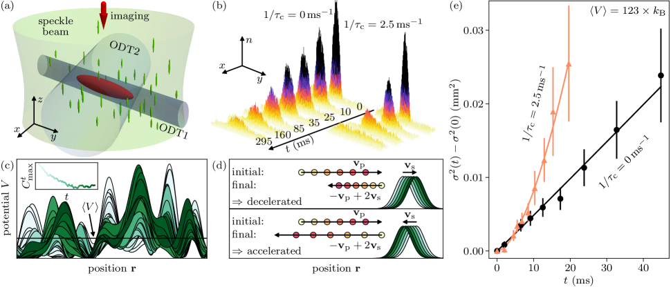
Figure 1: Experimental setup and analysis methods. (a) Sketch of atom cloud (large red ellipsoid), optical dipole traps (ODT1, blue cylinder along $y$ axis and ODT2, larger blue cylinder in $x$-$y$ plane), speckle laser beam (green volume), and anisotropic speckle grains (small green ellipsoids). Absorption imaging along the $-z$ direction (red arrow) is used to measure the cloud’s column density. (b) Surface plot of recorded density distribution for different expansion duration $t$ for $1/\tau_{\mathrm{c}}{}=$0\text{\,}{\mathrm{ms}}^{-1}$$ (left) and $1/\tau_{\mathrm{c}}{}=$2.5\text{\,}{\mathrm{ms}}^{-1}$$ (right). Shown are image sections with a full length along the $y$ axis of $1\text{\,}\mathrm{mm}$. For each setting of $t$ and $1/\tau_{\mathrm{c}}{}$, 50 repetitions have been taken and averaged. For increased visibility, the density data shown here was smoothed with a Gaussian filter with a standard deviation of one pixel. (c) Visualization of the disorder’s time evolution from a one-dimensional numerical simulation. Lines are snapshots along the evolution filled with lighter to darker green areas between successive time steps. Note how both peak heights and positions vary with different rates. The black horizontal line marks the average disorder potential $\langle V\rangle$, which is constant in $t$. The inset shows the cross-correlation peak height $C^{t}_{\mathrm{max}}$ in arbitrary units versus time $t$ (same color scale). The cross-correlation was calculated between the potential after duration $t$ and the first realization at $t=0$ as a measure of their similarity [39, 40]. (d) Illustration of Fermi acceleration in stroboscopic time evolution (from lighter to darker colors along time evolution). Rear-end collisions (top) effectively decelerate, while head-on collisions accelerate the particle. (e) Evolution of measured cloud variance over time from the two data sets shown in (b). Power-law fits (lines) to the data (points) yield diffusion exponents of $\alpha=1.02\,\pm\,0.04$ for $1/\tau_{\mathrm{c}}{}=$0\text{\,}{\mathrm{ms}}^{-1}$$ (circles) and $\alpha=1.70\,\pm\,0.08$ for $1/\tau_{\mathrm{c}}{}=$2.5\text{\,}{\mathrm{ms}}^{-1}$$, a clear indication of superdiffusion for the latter. Error bars indicate $1\sigma$ statistical uncertainty.

Here, we investigate the expansion of an ultracold non-interacting Fermi gas in a time-varying disorder potential to study the influence of the competing contributions of localization due to matter-wave interference and the acceleration due to stochastic Fermi acceleration on the diffusion of the gas. Depending on the decorrelation time of the disorder, i.e., the rate at which the disorder changes in time, we can tune our system through different regimes of anomalous diffusion ranging from subdiffusion arising due to localization effects, $\alpha<1$, continuously up to ballistic superdiffusion, $\alpha\approx 2$. Importantly, we observe an intermediate regime in which we find a strong suppression of the acceleration mechanism up to a critical rate, which we attribute to the effect of localization when matter-wave interference can still be maintained in the time-varying disorder potential.

Experimentally, we start by producing a degenerate Fermi gas of ⁶Li atoms at a temperature $T\approx$100\text{\,}\mathrm{n}\mathrm{K}$\approx$0.15\text{\,}$\,T_{\mathrm{F}}$, with Fermi temperature $T_{\mathrm{F}}=E_{\mathrm{F}}/k_{\mathrm{B}}$, Fermi energy $E_{\mathrm{F}}$ and Boltzmann constant $k_{\mathrm{B}}$. All $N\approx 10^{5}$ atoms are prepared spin-polarized in the lowest-lying Zeeman substate. Our sample behaves in good approximation as an ideal Fermi gas due to its fermionic nature, as $s$-wave interactions are prohibited entirely due to the Pauli exclusion principle and $p$-wave and higher-order interactions are strongly suppressed at these low temperatures [29]. Initially, the atoms are prepared in a trap created by superposing the main optical dipole trap (ODT1), formed by a focused laser beam propagating along the $y$ axis, with a secondary beam (ODT2), crossing the main beam at an angle in the $x$-$y$ plane, see Fig. 1(a). By extinguishing the ODT2 at time $t=0$, the trap instantly becomes shallow along the $y$ axis while the remaining directions are effectively unchanged. Hence, the atoms start to expand along the $y$-direction, see Fig. 1(b). After a variable expansion duration, we extract information about the cloud’s extension by performing absorption imaging along the $z$ axis [41, 42].

Simultaneously to switching off the ODT2, at $t=0$, we quench on a repulsive optical speckle disorder potential $V(\mathbf{r})$, created by $532\text{\,}\mathrm{nm}$ laser light, see Refs. [42, 39, 40] for details. Spatially, it consists of anisotropic grains with typical sizes of $\eta_{x,y}^{2}\times\eta_{z}=($750\text{\,}\mathrm{nm}$)^{2}\times$10.2\text{\,}\mathrm{\SIUnitSymbolMicro m}$$, where $\eta_{x,y}$ and $\eta_{z}$ are the correlation lengths along the respective directions [42, 43, 44]. We characterize the strength of the disorder by its spatial average $\langle V\rangle$. Technically, we can tune the rate $1/\tau_{\mathrm{c}}{}$ at which the disorder decorrelates and another speckle realization emerges that shares no resemblance to the original, see Fig. 1(c). While the local details of the disorder potential change significantly with time, its statistical properties, such as correlation length or mean potential, do not. Hence, we realize a time-varying stochastic force field for our atom cloud, allowing for stochastic Fermi acceleration (Fig. 1(d)), for details see Refs. [39, 40]. In the following, we realize decorrelation rates up to $1/\tau_{\mathrm{c}}{}=$3.5\text{\,}{\mathrm{ms}}^{-1}$$ to study the effect on the diffusion of non-interacting atoms in either weak ($\langle V\rangle=$123\text{\,}\mathrm{n}\mathrm{K}$\times k_{\mathrm{B}}\approx 0.2\,E_{F}$) or stronger ($\langle V\rangle=$401\text{\,}\mathrm{n}\mathrm{K}$\times k_{\mathrm{B}}\approx 0.5\,E_{F}$) disorder, see Appendix A. We note that, even in the static case, our three-dimensional disorder potential does not allow for any classically bound states [45, 46]. We further emphasize that the atom cloud never crosses into the regimes of dimensionality lower than $d=3$. Nevertheless, we still analyze the diffusive expansion only along one dimension, $d=1$, as the atoms are prohibited from expanding along the $x$ and $z$ directions.

From the absorption images taken, we extract the width $\sigma$ of the cloud. While standard methods such as the fitted Gaussian width or the participation ratio work in principle, we use the so-called inverse participation width (see Appendix B and Ref. [47] for details), which is particularly suited to compensate for noise of the imaging process, becoming relevant for long expansion times, when the local density of the cloud decreases.

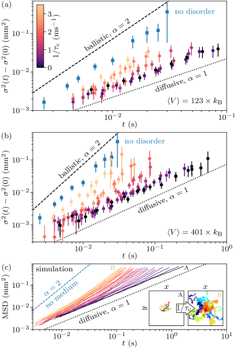
Figure 2: Tunable anomalous diffusion in dynamic disorder. Cloud variances from experimental data (points) for different decorrelation rates, increasing from $1/\tau_{\mathrm{c}}{}=$0\text{\,}{\mathrm{ms}}^{-1}$$ to $1/\tau_{\mathrm{c}}{}=$3.5\text{\,}{\mathrm{ms}}^{-1}$$ (color bar in (a)) for (a) weak disorder, $\langle V\rangle=$123\text{\,}\mathrm{n}\mathrm{K}$\times k_{\mathrm{B}}$, and (b) strong disorder, $\langle V\rangle=$401\text{\,}\mathrm{n}\mathrm{K}$\times k_{\mathrm{B}}$. Blue squares show variances from disorder-free, i.e., ballistic expansion. Error bars indicate $1\sigma$ statistical uncertainty. The black dotted (dashed) line indicates the exponent $\alpha$ for normal (ballistic) diffusion. (c) Particle-averaged mean squared displacement (MSD) from a single simulation run. We simulated 25 different velocity scales of the medium, ranging from the static case (A) to the experimentally maximum-achievable dynamics (B) in the same color scale as for the experimental data. The dashed blue line shows free expansion without a medium. Inset: twelve examples of simulated trajectories up to $t=$100\text{\,}\mathrm{ms}$$ for the static (A, left) and maximally dynamic case (B, right) from which we calculate MSD. Both boxes show an area of size $$1\text{\,}\mathrm{mm}$\times$1\text{\,}\mathrm{mm}$$. See Appendix C for more details on the simulation.

In Fig. 2, the cloud variances $\sigma^{2}$ over time are shown in a double-logarithmic plot for (a) weak and (b) strong disorder, where the exponent $\alpha$ of a power-law Eq. (1) corresponds to the slope of a straight line. The data from the expansion inside static disorder, $1/\tau_{\mathrm{c}}{}=$0\text{\,}{\mathrm{ms}}^{-1}$$, is shown as black points. It exhibits the lowest exponent for both disorder strengths, allowing for the longest observation times. The observation time is technically limited by atom losses or the finite size of the camera detection area and the envelope of the disorder speckle pattern. When we increase the decorrelation rate toward its maximum value of $1/\tau_{\mathrm{c}}{}=$3.5\text{\,}{\mathrm{ms}}^{-1}$$, we observe a strongly increased slope and, therefore, exponent for both disorder strengths. In fact, the exponent even takes on the same value as in the disorder-free expansion, i.e., ballistic transport.

To compare the experimental data to expectations derived from Fermi acceleration, we perform a Markov-chain Monte-Carlo simulation using a minimal stochastic model for Fermi acceleration based on Ref. [48], see Appendix for details. The resulting trajectories are used to compute a mean-squared displacement of the simulated particle, see Fig. 2(c). The simulation yields essentially the same accelerating behavior as seen in the experimental data.

A quantitative analysis of the change of dynamical regimes seen in Fig. 2 is done by extracting the diffusion exponent $\alpha$ and diffusion coefficient $D_{\alpha}$ from the different series of each $\langle V\rangle$ and $1/\tau_{\mathrm{c}}{}$. The exponent $\alpha$ is obtained as the slope from linear regression of the logarithm of both variance and time. With that, we calculate the anomalous diffusion coefficient as

$$D_{\alpha}=\left\langle\frac{\sigma_{i}^{2}(t)-\sigma_{i}^{2}(0)}{2t^{\alpha}}\right\rangle,$$ (2)

where the set of values that are averaged is constant in time. Note that $D_{\alpha}$ has the unit $\mathrm{m}^{2}\,\mathrm{s}^{-\alpha}$ [10].

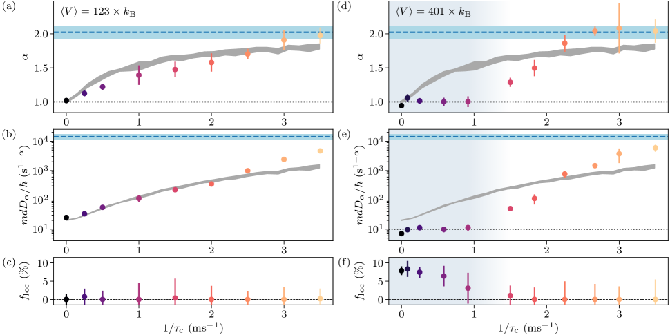
Figure 3: Diffusion properties for dynamic disorder. Left column (a-c) for weak disorder, $\langle V\rangle=$123\text{\,}\mathrm{n}\mathrm{K}$\times k_{\mathrm{B}}$, and right column (d-f) strong disorder, $\langle V\rangle=$401\text{\,}\mathrm{n}\mathrm{K}$\times k_{\mathrm{B}}$. (a, d) Diffusion exponents $\alpha$ as a function of decorrelation rate $1/\tau_{c}$ from experimental measurements (dots) and simulation data of twelve trajectories (gray area). The blue dashed line indicates ballistic, free-expansion measurement, and the blue area around it shows its error. Experimental error bars for dots and simulation-data area indicate $1\sigma$ statistical uncertainty. (b, e) Diffusion coefficient $D_{\alpha}$, normalized by $\hbar/m$ and expansion dimension $d$ with the same colors and line types as in panel (a). For the experimental data, $d=1$, and for the simulation, $d=2$, see Appendix C for details. Experimental errors are calculated as the standard deviation of values used for averaging, see Eq. (2). (c, f) Localized fraction $f_{\mathrm{loc}}$. For weak disorder, (c), it is consistent with zero for all decorrelation rates. For strong disorder, (f), we observe a significant $f_{\mathrm{loc}}>0$, which vanishes at $1/\tau_{\mathrm{c}}{}\approx$1\text{\,}{\mathrm{ms}}^{-1}$$, coinciding with the transition from a constant to a significant increase in both the diffusion exponent and coefficient. This quantum-transport region is highlighted by background shading in (d-f).

For the expansion in weak disorder, we see a direct and monotonous increase of both $\alpha$ and $D_{\alpha}$ with $1/\tau_{\mathrm{c}}{}$, see Fig. 3(a, b). Focusing on the exponent, we can tune through the entire range of superdiffusion with exponents between $\alpha=1$ for static, weak disorder and $\alpha=2$ by choice of $1/\tau_{\mathrm{c}}{}$. The simulation predicts this tunability well, even agreeing quantitatively with the experimental data for a wide range of decorrelation rates.

Turning to the results for the expansion in strong disorder, we find a strikingly different behavior. For static disorder, $1/\tau_{\mathrm{c}}{}=$0\text{\,}{\mathrm{ms}}^{-1}$$, we find the system to be slightly but statistically significantly in the subdiffusive regime with $\alpha=0.94\,\pm\,0.03$, see Fig. 3(d). As reported by Ref. [29], subdiffusion is expected to occur near the mobility edge until the wave packet has expanded into its fully localized state. A widely used estimate to discern if a system would be expected to be in the regime of Anderson localization is the Ioffe-Regel criterion, which can be expressed for ⁶Li as $T<$160\text{\,}\mathrm{n}\mathrm{K}$$ for the geometric mean of the correlation lengths $\overline{\eta}$ of our speckle disorder ($T<$900\text{\,}\mathrm{n}\mathrm{K}$$ for $\eta_{x,y}$ relevant for the expansion direction) [28]. As the gas temperature is $T\approx$100\text{\,}\mathrm{n}\mathrm{K}$$, our system fulfills the Ioffe-Regel criterion. An alternative criterion regards the critical momentum $k_{\mathrm{AL}}$ below which Anderson localization is expected to occur [49]. Specifically for our case $\langle V\rangle/E_{\mathrm{c}}>1$, with correlation energy $E_{\mathrm{c}}=\hbar^{2}/(m\eta^{2})$, we use the estimation $k_{\mathrm{AL}}\approx(\langle V\rangle/E_{\mathrm{c}})^{2/5}/\eta$, where $\hbar$ is the reduced Planck constant and $m$ is the atom mass. By comparison with the Fermi momentum $k_{\mathrm{F}}$, the largest momentum present in our degenerate Fermi gas, we get $k_{\mathrm{F}}\approx 2\,k_{\mathrm{AL}}$ for $\overline{\eta}$ (and $k_{\mathrm{F}}\approx 0.8\,k_{\mathrm{AL}}$ for $\eta_{x,y}$). In any case, we should expect at least a significant fraction of the low-energy fermions to localize. Therefore, we attribute the onset of subdiffusion for strong disorder as a signature of Anderson localization below the mobility edge, slowing down the expansion, see Ref. [47].

This is supported by the experimental observation that the diffusion coefficient is of the order of only a few ‘quanta of diffusion’ $\hbar/m$ [44, 27, 29], see Fig. 3(e). Furthermore, with increasing $1/\tau_{\mathrm{c}}{}{}\lesssim$1\text{\,}{\mathrm{ms}}^{-1}$$, we see an initial plateau where neither diffusion quantity, exponent or coefficient, changes (background shading in Fig. 3(c-d)). It clearly illustrates a strong suppression of the Fermi acceleration for sufficiently slow changes of the underlying disorder potential. The experimental observation is also in stark contrast to the classical simulation based on Fermi acceleration. We interpret this observation as the effect of localization due to wavefunction interference for small decorrelation rates.

To investigate the interplay of localization effects with superdiffusion or its suppression more closely, we infer a measure for the fraction $f_{\mathrm{loc}}$ of localized atoms as introduced in Ref. [27]. It quantifies the fraction of particles that would not have diffused away from the initial cloud volume after infinite time, see Appendix D and Ref. [47] for more details. We find a localized fraction of zero for the expansion in weak disorder even in the static case, as expected and can be seen in Fig. 3(c). By contrast, we find a significant localized fraction $f_{\mathrm{loc}}=$7.9\pm 1.2\text{\,}\%$$ for the strong static disorder, see Fig. 3(f). As expected, the fraction decays as the decorrelation rate $1/\tau_{\mathrm{c}}{}$ increases, but as long as a localized fraction persists, the system shows close-to-normal diffusion. However, the normal-diffusion plateau ends as soon as the localized fraction has decayed.

We interpret this plateau of $\alpha$ and $D_{\alpha}$ as a consequence of localization effects stabilizing diffusion against the disorder’s accelerating dynamics. In fact, the energy scale $h/\tau_{\mathrm{c}}\approx$48\text{\,}\mathrm{n}\mathrm{K}$\times k_{\mathrm{B}}$ for the observed delocalization rate $1/\tau_{\mathrm{c}}{}\approx$1\text{\,}{\mathrm{ms}}^{-1}$$ is of the same order of magnitude as the energy associated with the critical momentum for Anderson localization, being $E_{\mathrm{AL}}=\hbar^{2}k_{\mathrm{AL}}^{2}/2m\approx$115\text{\,}\mathrm{n}\mathrm{K}$\times k_{\mathrm{B}}$ for the strong disorder and $\overline{\eta}$. Therefore, the fraction of particles with sufficiently low energy to localize despite the additional energy $E_{\mathrm{AL}}$ will be increasingly reduced with $1/\tau_{\mathrm{c}}{}$ until too few low-energy particles remain to influence the transport globally. Around $1/\tau_{\mathrm{c}}{}\approx$1\text{\,}{\mathrm{ms}}^{-1}$$, where $f_{\mathrm{loc}}$ has vanished, the Fermi acceleration becomes too strong to sustain coherent matter-wave interference and finally drives the system to superdiffusion.

Our experimental study has provided insights into the interplay between Anderson localization and Fermi acceleration within the context of quantum transport. We have demonstrated a system that exhibits a broad tunability of anomalous diffusion, ranging from subdiffusion to superdiffusion, while reaching the regime of ballistic transport. Our findings elucidate the intriguing dynamics of matter waves in time-varying random force fields, establishing an experimental platform to investigate Fermi acceleration in quantum systems. An interesting prospect will be to reveal the criterion when Anderson localization breaks down and Fermi acceleration sets in more closely. Furthermore, achieving decorrelation timescales below the inverse Fermi energy could allow access to the regime of hyper transport, which will allow us to experimentally explore the maximum achievable acceleration rate in Fermi acceleration. Moreover, it will be interesting in future studies to explore the contributions of particle interactions or superfluidity, as our system is generally capable of creating a strongly interacting Fermi gas along the crossover from a molecular Bose-Einstein condensate (BEC) to a Bardeen-Cooper-Schrieffer (BCS) superfluid [41, 50]. Finally, this degree of tunable anomalous diffusion might be of value in related applications of wave phenomena, such as atomtronics, electronics, and (electro)chemical settings, where precise control over the transport velocity would be highly desirable.

We thank M. Fleischhauer, C. A. R. Sá de Melo, A. Buchleitner, T. Enss, D. Hernández-Rajkov, G. Roati, and E. Lutz for discussions as well as B. Moser, I. Cardoso Barbosa, and B. Nagler for carefully reading the manuscript. This work was supported by the German Research Foundation (DFG) through the Collaborative Research Center Sonderforschungsbereich SFB/TR185 (Project 277625399). M.K.-E. acknowledges support by the Quantum Initiative Rhineland-Palatinate QUIP. J.K. acknowledges support by the Max Planck Graduate Center with the Johannes Gutenberg-Universität Mainz.

Author contributions.

S.B. and A.W. conceived the research. S.B., F.L., and J.K. ran the experimental apparatus. S.B. took and analyzed the experimental data. M.K.-E. contributed to the analysis. S.B. wrote and analyzed the Monte-Carlo simulation. All authors contributed to the interpretation of the data, writing of the manuscript and critical feedback.

Competing interests.

The authors declare no competing interests.

Data availability.

All data of the figures in the manuscript and Methods are available in a Zenodo repository: https://zenodo.org/doi/10.5281/zenodo.10478890 (Ref. [51]).

Code availability.

The codes that support the findings of this paper are available from the corresponding author upon reasonable request.

Appendix A Experimental details

Our experimental sequence for the preparation of the spin-polarized gas, the trap configuration, gas temperature, and imaging are based on previous work Ref. [47]. We employ resonant high-intensity absorption imaging, see Refs. [52, 42]. Before the spin polarization, we evaporatively cool a previously laser-cooled sample of ⁶Li atoms in the two lowest Zeeman substates to temperatures around $T=$100\text{\,}\mathrm{n}\mathrm{K}$$ [41]. The evaporation takes place at a magnetic field of $B=$763.6\text{\,}\mathrm{G}$$, on the BEC side of the broad Feshbach resonance, which allows us to tune the interaction strength of the gas such that the cooling is efficient [53, 54]. Afterward, we adiabatically ramp the magnetic field to $B=$1070\text{\,}\mathrm{G}$$, deep into the BCS regime, where the fermionic pairs are weakly bound and spatially far apart. All atoms in one of the spin states are then removed from the trap by a resonant laser pulse, leaving a spin-polarized sample forming a quasi-pure Fermi sea. Only about $10\text{\,}\%$ of the atoms in the lowest-lying state are lost due to resonant scattering, while no measurable amount in the other state remains.

Since the magnetic field’s curvature strongly traps the atoms in the $x$-$y$ plane while being anti-confining along the $z$ axis [43], we load the atoms into the crossed dipole trap as shown in Fig. 1, and switch off the magnetic field. At that point, we can either extract the cloud’s temperature with the method described in Refs. [55, 56] or begin the expansion sequence by switching off ODT2 while switching on the disorder potential, both during less then one microsecond using acousto-optical modulators, faster than the timescale of the motion of the atoms. We ensured that, for every step of the preparation sequence, no observable excitations are performed and no significant amount of atoms are lost, the only exception being the polarization pulse as mentioned.

When driving the system with non-zero correlation rates, we observed that atoms were so strongly accelerated that the cloud expanded significantly along the $x$ direction. Therefore, we increased the power of the ODT1 laser from $100\text{\,}\mathrm{mW}$, as was used for the weak disorder in this work and for the entirety of Ref. [47], to $300\text{\,}\mathrm{mW}$. The resulting trap parameters for the series with weak disorder amount to $(\omega_{x},\omega_{y},\omega_{z})=(365,1.9,248)\times 2\pi\,$\text{\,}\mathrm{H}\mathrm{z}$$ after $t=0$ and, with that, $E_{\mathrm{F}}\approx$600\text{\,}\mathrm{n}\mathrm{K}$\times k_{\mathrm{B}}$ as well as $\langle V\rangle/E_{\mathrm{F}}\approx 0.2$. For the strong-disorder measurements, $(\omega_{x},\omega_{y},\omega_{z})=(670,3.4,435)\times 2\pi\,$\text{\,}\mathrm{H}\mathrm{z}$$, from which we calculate $E_{\mathrm{F}}\approx$850\text{\,}\mathrm{n}\mathrm{K}$\times k_{\mathrm{B}}$ as well as $\langle V\rangle/E_{\mathrm{F}}\approx 0.5$. Note that, for both series, $\omega_{y}=37.8\times 2\pi\,$\text{\,}\mathrm{H}\mathrm{z}$$ for $t<0$. We confirmed that the disorder-free expansion is still ballistic. For sufficiently slow dynamics, the expansion in strong disorder is very similar for both trap configurations. The energy can be dissipated into the unobserved directions only for the larger decorrelation rates, effectively reducing the superdiffusion along $y$.

Appendix B Determination of the cloud variance

We use the inverse participation width (IPW), a statistical observable introduced in our previous work Ref. [47], as a measure for the cloud’s spatial extension. For that, we calculate the histogram of an absorption image taken at time $t$, approximating the particle’s position probability density function (PDF), and extract its width $w(t)$ as the full range between the largest and lowest recorded densities. As camera noise is present and influences the recorded histogram, we have to take it into account. For that, we also extract the width $w_{\mathrm{noise}}$ of a histogram of a noisy image without any atoms but otherwise identical statistics. More precisely, the recorded histogram will be the convolution of the noise-free distribution, a bimodal function for most settings, with the PDF of the camera noise. In cases such as ours, $w(t)-w_{\mathrm{noise}}$ will then be a good approximation for the sample’s peak density $n(0,t)$. Assuming that the cloud spreads as $n(0,t)\sim N(t)/\sigma$, we get the cloud variance from IPW as

$$\sigma^{2}(t)\approx\frac{1}{2\pi}\frac{N^{2}(t)}{(w(t)-w_{\mathrm{noise}})^{2}}.$$ (3)

Here, we have already inserted the squared prefactor $1/2\pi$ from a Gaussian function to allow a quantitative analysis of the diffusion coefficient. We emphasize that the prefactor choice is unimportant for our conclusions because even using a box distribution (which is obviously significantly different from our cloud shape), for example, will yield $1/4$, which is still somewhat comparable to $1/2\pi\approx 0.16$. The coefficient can therefore be extracted with an uncertainty of order unity. To determine the diffusion exponent quantitatively, only $n(0,t)\sim N(t)/\sigma(t)$ needs to be valid. For details about IPW, its regimes of validity, and a comparison with established observables, see Ref. [47].

Appendix C Fermi-acceleration simulation

As stated in the main text, the simulations are based on the model presented in Ref. [48]. We simulate classical non-relativistic point particles colliding elastically with hard-sphere scatterers of infinite mass on a flat two-dimensional plane. We choose a 2D system since, in 1D, the mechanism of Fermi acceleration is significantly different due to the lack of scattering angles. Single scattering events are effectively the same for dimensions larger than one if the scattering angles are assumed uniformly distributed. Since our atom cloud is three-dimensional, we simulate in $d>1$ and choose $d=2$ as a compromise to save computing resources.

In the case of frozen scattering centers, normal diffusion is the result. However, when these scatterers themselves are moving, the particles undergo Fermi acceleration and expand superdiffusively. Since here and in contrast to the experimental setup, we do have access to the trajectories $\mathbf{r}(t)$ of each particle, we directly calculate the mean-squared displacement as

$$\mathrm{MSD}(t)=\langle\mathbf{r}^{2}\rangle(t)-\langle\mathbf{r}^{2}\rangle(0),$$ (4)

where $\langle\cdot\rangle$ denotes the average over the particles. For each simulation run, we set $1000\text{\,}$ particles, each colliding $25\,000\text{\,}$ times with the randomly moving spheres. Finally, we run such a series twelve times and average the diffusion exponents and coefficients extracted from each series.

We choose values as close to the experimental setting as possible for the scatterers. As their radius, we use the geometric mean of our disorder’s correlation lengths $\overline{\eta}$ and use the average distance of speckle peaks, $3\overline{\eta}$, for their density $\rho=1/(3\,\overline{\eta})^{2}$. Since the speckle’s spatial intensity is exponentially distributed, we assumed that the same holds for the velocity. Therefore, the simulated scatterers’ velocity is determined randomly with an exponential probability distribution. Note that the choice of their velocity distribution has little to no impact on the result. Only the average velocity has a significant influence. Therefore, we iterate through 25 different values of their average velocity between zero (see black line A in Fig. 2(c)) and the maximum value (yellow line B) of $v_{\mathrm{sim}}^{\mathrm{max}}=$6.3\text{\,}\mathrm{mm}\text{\,}{\mathrm{s}}^{-1}$$. That value is estimated from the velocity scale of our maximally dynamic disorder by comparing the present length and timescales $\overline{\eta}/\tau_{\mathrm{c}}$ for $1/\tau_{\mathrm{c}}{}=$3.5\text{\,}{\mathrm{ms}}^{-1}$$. For the initial spatial distribution of the point particles, we choose a Gaussian with $\sigma_{x,y}(0)=$50\text{\,}\mathrm{\SIUnitSymbolMicro m}$$. For their velocity magnitudes, we distribute values between zero and the Fermi velocity $v_{\mathrm{F}}$ of our experimental system as they would be for an ideal Fermi gas, while the angles are chosen isotropically. Note that, except for the cases of static (where only the direction but not the magnitude of the velocity vector can change) or absent scatterers, its choice has a negligible influence on the expansion due to the underlying Markov assumption.

Even though we insert the various scales of our experiment as closely as possible, we emphasize that the simulation still describes a very different setting from our system. Nevertheless, employing the simulation reinforces the assumption that Fermi acceleration is the underlying mechanism driving our atoms to superdiffusion.

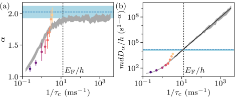
Figure 4: Results from extended simulation for (a) exponent $\alpha$ and (b) diffusion coefficient $D_{\alpha}$ in analogy to Fig. 3, but with extended decorrelation rates up to $1/\tau_{\mathrm{c}}{}=$3.5\text{\,}{\mathrm{ms}}^{-1}$$. The graph shows the combined data from the original and extended simulations on a logarithmic $1/\tau_{\mathrm{c}}{}$ axis together with the experimental results from the expansion in weak disorder, $\langle V\rangle=$123\text{\,}\mathrm{n}\mathrm{K}$\times k_{\mathrm{B}}$. Blue dashed lines and areas around it show the experimental results of the disorder-free expansion. The black dotted line marks $E_{\mathrm{F}}/h$, and the black solid line in (b) is a power-law fit to the simulation yielding an exponent of $\nu_{\mathrm{FA}}=1.98\,\pm\,0.02$.

To investigate the maximally achievable exponent, we extend our simulation series in $1/\tau_{\mathrm{c}}{}$ by three orders of magnitude, see Fig. 4(a). As observed from our simulation data, the exponent approaches $\alpha=2$ for large $1/\tau_{\mathrm{c}}{}$. As stated by Ref. [48], $\alpha=2$ is the expected scaling law for infinite time, which we appear to approximate closely albeit slowly. For any experimental system with finite size and disorder strength, the ballistic exponent $\alpha=2$ will be the limit if enough time has passed. This can be intuitively understood in finite-amplitude disorder, where, after sufficient acceleration, particles will have energies above the large majority of the disorder, and the acceleration saturates. Effectively, there are hardly any potential features high enough to accelerate the particle further. On the other side, as was shown in Refs. [7, 4, 5], even exponents $\alpha>2$ beyond the ballistic regime, called hyper transport, can be expected inside dynamic disorder.

We compare the relevant present rates and inverse timescales to estimate the efficiency with which we can increase the energy in our experimental system. For the maximally dynamic disorder, local disorder dynamics occur with the decorrelation rate of $\tau_{\mathrm{c}}=$3.5\text{\,}{\mathrm{ms}}^{-1}$$ [39]. The Fermi energy corresponds to the inverse timescale $E_{\mathrm{F}}/h\approx$12.5\text{\,}{\mathrm{ms}}^{-1}$$, where $h$ is the Planck constant, i.e., it is larger by a factor of roughly $3.5$, see Fig. 4. Around that rate, the exponent from the simulation begins to saturate, while the diffusion coefficient coincides with the experimentally determined $D_{2}$ from the disorder-free expansion. Alternatively, we can estimate the optimal rate $1/\tau_{\mathrm{opt}}\approx$10.5\text{\,}{\mathrm{ms}}^{-1}$$ to drive superdiffusion as efficiently as possible, as described in Ref. [6] for a classical two-dimensional system, yielding a similar factor. Thus, both comparisons indicate that we could enhance the rate of energy increase if we were to achieve higher decorrelation rates, which is technically not possible yet. Additionally, we find that the diffusion coefficient for decorrelation rates $1/\tau_{c}\geq E_{\mathrm{F}}/h$ follows a power law with exponent $\nu_{\mathrm{FA}}\approx 2$, see Fig. 4(b). Since the kinetic energy $E_{\mathrm{kin}}\sim v_{\mathrm{p}}^{2}\sim D_{2}$ of a particle with velocity $v_{\mathrm{p}}$ increases with $1/\tau_{\mathrm{c}}{}^{\nu_{\mathrm{FA}}}\sim v_{\mathrm{s}}^{\nu_{\mathrm{FA}}}$ (with average scatterer velocity $v_{\mathrm{s}}$, see Fig. 1(d)), we recover $E_{\mathrm{kin}}\sim v_{\mathrm{s}}^{2}$, which is the expected scaling for second-order Fermi acceleration [33, 48].

Appendix D Localized fraction

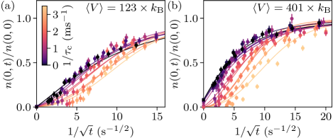
Figure 5: Determining the localized fraction $f_{\mathrm{loc}}$ from the series with (a) weak disorder, $\langle V\rangle=$123\text{\,}\mathrm{n}\mathrm{K}$\times k_{\mathrm{B}}$, and (b) strong disorder, $\langle V\rangle=$401\text{\,}\mathrm{n}\mathrm{K}$\times k_{\mathrm{B}}$. Plotting the relative density $n(t)/n(0)$ (circles) over the square root of inverse time allows us to visualize $f_{\mathrm{loc}}$ as the density-axis intercept (crosses). Lines are fits with the anomalous-diffusion model Eq. (5) where $f_{\mathrm{loc}}$, the value of the density for $t\rightarrow\infty$, is the only free parameter. Errors are calculated from error propagation.

The localized fraction $f_{\mathrm{loc}}$ estimates the infinite-time fraction of atoms that would not diffuse away due to being localized, assuming no atom losses. We base the determination of the localized fraction on the method reported in Ref. [27]. We modified it to fit our expansion along a single dimension and implemented the full anomalous-diffusion power law as in Eq. (1). More precisely, we use the model

$$\frac{n(0,t)}{n(0,0)}=f_{\mathrm{loc}}+(1-f_{\mathrm{loc}})\sqrt{\frac{\sigma^{2}(0)}{2D_{\alpha}t^{\alpha}+\sigma^{2}(0)}},$$ (5)

where we fix the diffusion exponent $\alpha$ and coefficient $D_{\alpha}$ to the values we extract as described in the text and use $\sigma(0)=$53\text{\,}\mathrm{\SIUnitSymbolMicro m}$$ from a Gauss fit to the trapped cloud. For the relative peak density $n(0,t)/n(0,0)$, we use the above-mentioned approximation of $n(0,t)\approx w(t)-w_{\mathrm{noise}}$ with an additional factor of $N(0)/N(t)$ to compensate for atom losses. With that, $f_{\mathrm{loc}}$ is extracted as the only free parameter from fitting the right side of Eq. (5), see Fig. 5. Further, see Ref. [47] for more details.

References

- Anderson [1958] P. W. Anderson, Absence of Diffusion in Certain Random Lattices, Physical Review 109, 1492 (1958).
- Abrahams [2010] E. Abrahams, ed., 50 Years of Anderson Localization (World Scientific, Singapore, 2010).
- Fermi [1949] E. Fermi, On the Origin of the Cosmic Radiation, Physical Review 75, 1169 (1949).
- Jayannavar and Kumar [1982] A. M. Jayannavar and N. Kumar, Nondiffusive Quantum Transport in a Dynamically Disordered Medium, Physical Review Letters 48, 553 (1982).
- Golubović et al. [1991] L. Golubović, S. Feng, and F.-A. Zeng, Classical and quantum superdiffusion in a time-dependent random potential, Physical Review Letters 67, 2115 (1991).
- Volpe et al. [2014] G. Volpe, G. Volpe, and S. Gigan, Brownian Motion in a Speckle Light Field: Tunable Anomalous Diffusion and Selective Optical Manipulation, Scientific Reports 4, 3936 (2014).
- Levi et al. [2012] L. Levi, Y. Krivolapov, S. Fishman, and M. Segev, Hyper-transport of light and stochastic acceleration by evolving disorder, Nature Physics 8, 912 (2012).
- Einstein [1956] A. Einstein, Investigations on the Theory of the Brownian Movement, edited by R. Fürth (Dover Publications, 1956).
- Duplantier [2006] B. Duplantier, Brownian Motion, “Diverse and Undulating”, in Einstein, 1905–2005: Poincaré Seminar 2005, Progress in Mathematical Physics, edited by T. Damour, O. Darrigol, B. Duplantier, and V. Rivasseau (Birkhäuser, Basel, 2006) pp. 201–293.
- Metzler and Klafter [2000] R. Metzler and J. Klafter, The random walk’s guide to anomalous diffusion: a fractional dynamics approach, Physics Reports 339, 1 (2000).
- Muñoz-Gil et al. [2021] G. Muñoz-Gil, G. Volpe, M. A. Garcia-March, E. Aghion, A. Argun, C. B. Hong, T. Bland, S. Bo, J. A. Conejero, N. Firbas, î Garibo i Orts, A. Gentili, Z. Huang, J.-H. Jeon, H. Kabbech, Y. Kim, P. Kowalek, D. Krapf, H. Loch-Olszewska, M. A. Lomholt, J.-B. Masson, P. G. Meyer, S. Park, B. Requena, I. Smal, T. Song, J. Szwabiński, S. Thapa, H. Verdier, G. Volpe, A. Widera, M. Lewenstein, R. Metzler, and C. Manzo, Objective comparison of methods to decode anomalous diffusion, Nature Communications 12, 6253 (2021).
- Uchaikin and Sibatov [2017] V. Uchaikin and R. Sibatov, Fractional derivatives on cosmic scales, Chaos, Solitons & Fractals 102, 197 (2017).
- Viswanathan et al. [1996] G. M. Viswanathan, V. Afanasyev, S. V. Buldyrev, E. J. Murphy, P. A. Prince, and H. E. Stanley, Lévy flight search patterns of wandering albatrosses, Nature 381, 413 (1996).
- Edwards et al. [2007] A. M. Edwards, R. A. Phillips, N. W. Watkins, M. P. Freeman, E. J. Murphy, V. Afanasyev, S. V. Buldyrev, M. G. E. da Luz, E. P. Raposo, H. E. Stanley, and G. M. Viswanathan, Revisiting Lévy flight search patterns of wandering albatrosses, bumblebees and deer, Nature 449, 1044 (2007).
- Plerou et al. [2000] V. Plerou, P. Gopikrishnan, L. A. Nunes Amaral, X. Gabaix, and H. Eugene Stanley, Economic fluctuations and anomalous diffusion, Physical Review E 62, R3023 (2000).
- Balescu [1995] R. Balescu, Anomalous transport in turbulent plasmas and continuous time random walks, Physical Review E 51, 4807 (1995).
- Di Pierro et al. [2018] M. Di Pierro, D. A. Potoyan, P. G. Wolynes, and J. N. Onuchic, Anomalous diffusion, spatial coherence, and viscoelasticity from the energy landscape of human chromosomes, Proceedings of the National Academy of Sciences 115, 7753 (2018).
- Weaver [1990] R. Weaver, Anderson localization of ultrasound, Wave Motion 12, 129 (1990).
- Hu et al. [2008] H. Hu, A. Strybulevych, J. H. Page, S. E. Skipetrov, and B. A. van Tiggelen, Localization of ultrasound in a three-dimensional elastic network, Nature Physics 4, 945 (2008).
- Dalichaouch et al. [1991] R. Dalichaouch, J. P. Armstrong, S. Schultz, P. M. Platzman, and S. L. McCall, Microwave localization by two-dimensional random scattering, Nature 354, 53 (1991).
- Wiersma et al. [1997] D. S. Wiersma, P. Bartolini, A. Lagendijk, and R. Righini, Localization of light in a disordered medium, Nature 390, 671 (1997).
- Scheffold et al. [1999] F. Scheffold, R. Lenke, R. Tweer, and G. Maret, Localization or classical diffusion of light?, Nature 398, 206 (1999).
- Schwartz et al. [2007] T. Schwartz, G. Bartal, S. Fishman, and M. Segev, Transport and Anderson localization in disordered two-dimensional photonic lattices, Nature 446, 52 (2007).
- Mafi and Ballato [2021] A. Mafi and J. Ballato, Review of a Decade of Research on Disordered Anderson Localizing Optical Fibers, Frontiers in Physics 9 (2021).
- Billy et al. [2008] J. Billy, V. Josse, Z. Zuo, A. Bernard, B. Hambrecht, P. Lugan, D. Clément, L. Sanchez-Palencia, P. Bouyer, and A. Aspect, Direct observation of Anderson localization of matter waves in a controlled disorder, Nature 453, 891 (2008).
- Roati et al. [2008] G. Roati, C. D’Errico, L. Fallani, M. Fattori, C. Fort, M. Zaccanti, G. Modugno, M. Modugno, and M. Inguscio, Anderson localization of a non-interacting Bose–Einstein condensate, Nature 453, 895 (2008).
- Jendrzejewski et al. [2012] F. Jendrzejewski, A. Bernard, K. Müller, P. Cheinet, V. Josse, M. Piraud, L. Pezzé, L. Sanchez-Palencia, A. Aspect, and P. Bouyer, Three-dimensional localization of ultracold atoms in an optical disordered potential, Nature Physics 8, 398 (2012).
- Kondov et al. [2011] S. S. Kondov, W. R. McGehee, J. J. Zirbel, and B. DeMarco, Three-Dimensional Anderson Localization of Ultracold Matter, Science 334, 66 (2011).
- Shapiro [2012] B. Shapiro, Cold atoms in the presence of disorder, Journal of Physics A: Mathematical and Theoretical 45, 143001 (2012).
- Evensky et al. [1990] D. A. Evensky, R. T. Scalettar, and P. G. Wolynes, Localization and dephasing effects in a time-dependent Anderson Hamiltonian, The Journal of Physical Chemistry 94, 1149 (1990).
- Lorenzo et al. [2018] S. Lorenzo, T. Apollaro, G. M. Palma, R. Nandkishore, A. Silva, and J. Marino, Remnants of Anderson localization in prethermalization induced by white noise, Physical Review B 98, 054302 (2018).
- Sturrock [1966] P. A. Sturrock, Model of the High-Energy Phase of Solar Flares, Nature 211, 695 (1966).
- Ostrowski and Siemieniec-Oziȩbło [1997] M. Ostrowski and G. Siemieniec-Oziȩbło, Diffusion in momentum space as a picture of second-order Fermi acceleration, Astroparticle Physics 6, 271 (1997).
- Mertsch and Sarkar [2011] P. Mertsch and S. Sarkar, Fermi Gamma-Ray “Bubbles” from Stochastic Acceleration of Electrons, Physical Review Letters 107, 091101 (2011).
- Ulam [1961] S. M. Ulam, On some statistical properties of dynamical systems, in Contributions to Astronomy, Meteorology, and Physics, edited by J. Neyman (University of California Press, 1961) pp. 315–320.
- Lichtenberg and Lieberman [1983] A. J. Lichtenberg and M. A. Lieberman, Regular and Stochastic Motion, edited by F. John, J. E. Marsden, and L. Sirovich, Applied Mathematical Sciences, Vol. 38 (Springer, New York, NY, 1983).
- José and Cordery [1986] J. V. José and R. Cordery, Study of a quantum fermi-acceleration model, Physical Review Letters 56, 290 (1986).
- Seba [1990] P. Seba, Quantum chaos in the Fermi-accelerator model, Physical Review A 41, 2306 (1990).
- Nagler et al. [2022a] B. Nagler, M. Will, S. Hiebel, S. Barbosa, J. Koch, M. Fleischhauer, and A. Widera, Ultracold Bose Gases in Dynamic Disorder with Tunable Correlation Time, Physical Review Letters 128, 233601 (2022a).
- Hiebel et al. [2023] S. Hiebel, B. Nagler, S. Barbosa, J. Koch, and A. Widera, Characterizing quantum gases in correlated-disorder realizations using density-density correlations, arXiv:2306.16099 (2023).
- Gänger et al. [2018] B. Gänger, J. Phieler, B. Nagler, and A. Widera, A versatile apparatus for fermionic lithium quantum gases based on an interference-filter laser system, Review of Scientific Instruments 89, 093105 (2018).
- Nagler et al. [2020] B. Nagler, M. Radonjić, S. Barbosa, J. Koch, A. Pelster, and A. Widera, Cloud shape of a molecular Bose–Einstein condensate in a disordered trap: a case study of the dirty boson problem, New Journal of Physics 22, 033021 (2020).
- Nagler et al. [2022b] B. Nagler, S. Barbosa, J. Koch, G. Orso, and A. Widera, Observing the loss and revival of long-range phase coherence through disorder quenches, Proceedings of the National Academy of Sciences 119 (2022b).
- Kuhn et al. [2007] R. C. Kuhn, O. Sigwarth, C. Miniatura, D. Delande, and C. A. Müller, Coherent matter wave transport in speckle potentials, New Journal of Physics 9, 161 (2007).
- Pilati et al. [2010] S. Pilati, S. Giorgini, M. Modugno, and N. Prokof’ev, Dilute Bose gas with correlated disorder: a path integral Monte Carlo study, New Journal of Physics 12, 073003 (2010).
- Sanchez-Palencia et al. [2008] L. Sanchez-Palencia, D. Clément, P. Lugan, P. Bouyer, and A. Aspect, Disorder-induced trapping versus Anderson localization in Bose–Einstein condensates expanding in disordered potentials, New Journal of Physics 10, 045019 (2008).
- Barbosa et al. [2023] S. Barbosa, M. Kiefer-Emmanouilidis, F. Lang, J. Koch, and A. Widera, What can we learn from diffusion about Anderson localization of a degenerate Fermi gas?, arXiv:2311.07505 (2023).
- Bouchet et al. [2004] F. Bouchet, F. Cecconi, and A. Vulpiani, Minimal Stochastic Model for Fermi’s Acceleration, Physical Review Letters 92, 040601 (2004).
- Beilin et al. [2010] L. Beilin, E. Gurevich, and B. Shapiro, Diffusion of cold-atomic gases in the presence of an optical speckle potential, Physical Review A 81, 033612 (2010).
- Koch et al. [2023] J. Koch, K. Menon, E. Cuestas, S. Barbosa, E. Lutz, T. Fogarty, T. Busch, and A. Widera, A quantum engine in the BEC–BCS crossover, Nature 621, 723 (2023).
- [51] S. Barbosa, M. Kiefer-Emmanouilidis, F. Lang, J. Koch, and A. Widera, Zenodo repository: https://zenodo.org/doi/10.5281/zenodo.10478890.
- Reinaudi et al. [2007] G. Reinaudi, T. Lahaye, Z. Wang, and D. Guéry-Odelin, Strong saturation absorption imaging of dense clouds of ultracold atoms, Optics Letters 32, 3143 (2007).
- Grimm [2007] R. Grimm, Ultracold Fermi gases in the BEC-BCS crossover: a review from the Innsbruck perspective, arXiv:cond-mat/0703091 (2007).
- Zürn et al. [2013] G. Zürn, T. Lompe, A. N. Wenz, S. Jochim, P. S. Julienne, and J. M. Hutson, Precise Characterization of 6Li Feshbach Resonances Using Trap-Sideband-Resolved RF Spectroscopy of Weakly Bound Molecules, Physical Review Letters 110, 135301 (2013).
- Hadzibabic et al. [2002] Z. Hadzibabic, C. Stan, K. Dieckmann, S. Gupta, M. Zwierlein, A. Görlitz, and W. Ketterle, Two-species mixture of quantum degenerate bose and fermi gases, Physical Review Letters 88, 160401 (2002).
- Kinast [2006] J. M. Kinast, Thermodynamics and superfluidity of a strongly interacting Fermi gas, Ph.D. thesis, Duke University (2006).