Feedforward neural networks as statistical models: Improving interpretability through uncertainty quantification

Abstract

Feedforward neural networks (FNNs) are typically viewed as pure prediction algorithms, and their strong predictive performance has led to their use in many machine-learning applications. However, their flexibility comes with an interpretability trade-off; thus, FNNs have been historically less popular among statisticians. Nevertheless, classical statistical theory, such as significance testing and uncertainty quantification, is still relevant. Supplementing FNNs with methods of statistical inference, and covariate-effect visualisations, can shift the focus away from black-box prediction and make FNNs more akin to traditional statistical models. This can allow for more inferential analysis, and, hence, make FNNs more accessible within the statistical-modelling context.

Keywords. Neural networks; Hypothesis testing; p-values; Uncertainty quantification; Covariate-effect plots.

1 Introduction

Many applications require the estimation of a complex underlying relationship between a response variable and a set of explanatory variables. Often, and increasingly in recent years, neural networks have been used to approximate this relationship (LeCun et al.,, 2015). This has led to their application in a wide variety of fields, particularly those requiring high-performing predictive algorithms, such as finance, healthcare, and economics. However, while neural networks exhibit strong predictive capabilities, and are being used in high-stake decision making, they are viewed as “black-box” algorithms, i.e., their predictions are not easily understood and are difficult to interpret (Rudin,, 2019). For example, predictive models are crucial in the insurance industry. The ability to accurately predict a patient’s average medical care expenses would allow insurers to competitively price their premiums. However, as these models would be implemented in a decision-making process about an individual (i.e., using their personal data to forecast their medical expenses), regulatory requirements, such as the EU’s General Data Protection Regulation (GDPR), require an associated explanation (Samek and Müller,, 2019). This can limit, or even prohibit, the use of neural networks.

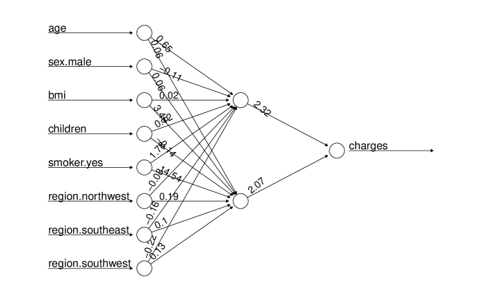
The insurance data (Lantz,, 2019) contains information relating to an insurance plan’s primary beneficiaries and the total amount of medical expenses charged to each account in the United States (measured in thousands of dollars). Whilst a quite simple, shallow neural network has strong performance in the prediction of the amount billed to each account, it does not offer any insights into the underlying relationship. (Note: a neural network with all covariates and two hidden nodes achieves a five-fold cross-validation root mean squared error of 4.634 ($\pm 0.144$); see Section 6 for more detail.) Indeed, most neural network software offers very little information beyond predictive performance metrics; summaries beyond out-of-sample performance are apparently of less concern in this context (Efron,, 2020). However, one could inspect the weight values learned by the neural network—a plot showing the values for each weight in the neural network fitted to the insurance data is given in Figure 1—but, on its own, this is not very useful, and it does not greatly improve our understanding of the model.

Instead of using black boxes, applications that require explainability typically turn to inherently interpretable models within the field of statistical modelling. The workhorse of statistical modelling—classical linear regression—is the cornerstone of model explainability, with its easily understood covariate effects and statistical tests. It does, however, have weaker predictive performance in general relative to more general models such as neural networks. Continuing with the motivating example, a linear regression model fitted to the insurance data results in a worse root mean squared error ($6.107\pm 0.146$) compared to the neural network, but it does provide a model summary, shown in Table 1, which is useful and familiar to statisticians. This table effectively answers two questions that naturally arise when modelling the relationship between a covariate and a response. First, is there any relationship? This is covered by the p-values, which test for statistically significant associations. Second, if there is a relationship, what is the nature of this relationship? This is covered by the regression coefficients, which give us an idea of the size and direction of the relationship. From Table 1, we can see that age, bmi, children and smoker are all highly statistically significant, and increased values for each variable are associated with higher total medical expenses charged, on average (for the case of smoker, an increased value corresponds to going from non-smoker to smoker).

Figure 1: Plot of neural network architecture for the insurance data with its associated weight values generated using the neuralnet package in R (Fritsch et al.,, 2019). Note that the continuous covariates and the response have been standardised for the purpose of optimisation stability.

Table 1: Summary of linear model for the insurance data.

	$\hat{\beta}_{j}$ (SE)	p-value
intercept	-11.939 (0.988)	$<0.001$
age	0.257 (0.012)	$<0.001$
sex.male	-0.131 (0.333)	0.693
bmi	0.339 (0.029)	$<0.001$
children	0.476 (0.138)	$<0.001$
smoker	23.849 (0.413)	$<0.001$
region.nw	-0.353 (0.476)	0.459
region.se	-1.035 (0.479)	0.031
region.sw	-0.960 (0.478)	0.045

The motivating example highlights the trade-off between model interpretability and model predictivity and also distinguishes between the traditional approaches of statistical modelling (focused on explanation) and machine learning (focused on prediction) (Shmueli,, 2010). These two fields have not developed in unison and the majority of neural network research has been conducted outside of the field of statistics (Breiman,, 2001; Efron and Hastie,, 2021; Hooker and Mentch,, 2021). As a result of this, other avenues toward explainability exist (see Guidotti et al., (2018) for a comprehensive review). Model-agnostic methods, i.e., methods that can be used on any black-box model, are a popular alternative (Ribeiro et al., 2016a, ). This includes methods that perturb inputs such as Shapley values (Strumbelj and Kononenko,, 2010) and local surrogate models such as Locally Interpretable Model Explanations (LIME) (Ribeiro et al., 2016b, ). However, one downfall of these methods is that they are not robust to small modifications of the inputs, and this instability can make their explanations difficult to trust (Alvarez-Melis and Jaakkola,, 2018).

In this paper, we treat shallow neural networks as statistical models, and aim to show how, and when, these models can be used as an alternative statistical non-linear regression model. We tackle the applied problem of interpreting neural networks using likelihood-based inferential techniques, and demonstrate that they are useful beyond pure prediction problems. The presence of a relationship between a covariate and the response will primarily be addressed through the multiple-parameter Wald test (since multiple network weights link each input to the hidden nodes). Although this test was discussed in the context of neural networks previously by White, (1989), to the best of our knowledge, it is never used in practice and has not been extensively tested. The reason it has not been used up to now is perhaps due to the issue of unidentifiability that can occur for the parameters in (more complex) neural networks; this can lead to issues in computing the variance-covariance matrix of the estimated parameters (Fukumizu,, 1996). Instead, asymptotic properties of neural networks have recently been based on non-parametric regression techniques such as the sensitivity-based approach proposed in Horel and Giesecke, (2020), or using neural network sieve estimators such as Shen et al., (2023). However, we take a more traditional approach, and make use of classical testing that, we believe, will be more familiar to statisticians in general. To overcome the issue with the Wald test, we extend it to the more modern setting of penalised estimation with the addition of a ridge penalty, which provides more stable estimation and improves its usability. When taking such an approach, one should use parsimonious models with identifiable parameters such that classical asymptotics can be applied, which can be achieved, for example, using the selection procedure of McInerney and Burke, (2022). Here, we carry out an empirical investigation to assess the estimation and inferential performance of Wald-based testing in neural networks. We also provide a convenient visualisation of the results from these tests, which are overlaid on the neural network architecture. Furthermore, the nature of statistically significant relationships will be addressed through covariate-effect plots that emulate regression coefficients, yielding interpretable model outputs that are more familiar in the statistical-modelling context.

The remainder of this paper is structured as follows. In Section 2, we introduce the feedforward neural network (FNN) model, and summarise some relevant likelihood theory. Section 3 discusses significance testing for input nodes (covariates) and individual weights (parameters). In Section 4, we propose covariate-effect plots that play a similar role to regression coefficients obtained from classical statistical models. The performance of the aforementioned methods is thoroughly investigated using simulation studies in Section 5. The motivating insurance data example is revisited throughout the paper, but will be explored in more detail in Section 6. Finally, we conclude with a discussion in Section 7.

2 Feedforward Neural Networks

Let $y_{i}$ be the response variable of interest, for $i=1,\dotsc,n$. We observe a vector of covariates, $x_{i}=(x_{i0},x_{i1},\dotsc,x_{ip})^{T}$, for the $i$th observation with covariates indexed by $j=0,1,\dotsc,p$, and $x_{i0}\equiv 1$. The general form of an FNN model can be written as

$$\mathbb{E}(y_{i}|x_{i})=\text{NN}(x_{i},\theta),$$

where

$$\text{NN}(x_{i},\theta)=\phi_{o}\left[\gamma_{0}+\sum_{k=1}^{q}\gamma_{k}\phi_{h}\left(\sum_{j=0}^{p}\omega_{jk}x_{ij}\right)\right],$$ (2.1)

and $\theta$ denotes the neural network parameters. The parameters are: $\omega_{jk}$, the weight that connects the $j$th covariate (input node) to the $k$th hidden node, where $\omega_{0k}$ is an intercept term; $\gamma_{k}$, the weight that connects the $k$th hidden node to the output node; and $\gamma_{0}$, the intercept term associated with the output node. Let $\omega_{j}=(\omega_{j1},\omega_{j2},\dotsc,\omega_{jq})^{T}$ be the vector representing all of the connection weights from input node $j$ to the hidden layer, and let $\gamma=(\gamma_{0},\gamma_{1},\dotsc,\gamma_{q})^{T}$ be the vector representing all of the connection weights between the hidden layer and the output layer. Finally, $\theta=(\omega_{0}^{T},\omega_{1}^{T},\dotsc,\omega_{p}^{T},\gamma^{T})^{T}$ is the vector of all parameters in the neural network model, which is of dimension $r=(p+2)q+1$. The function $\phi_{h}(\cdot)$ is the activation function for the hidden layer, which is often a logistic function, and the function $\phi_{o}(\cdot)$ is the activation function for the output layer. In the case where $y_{i}$ is a continuous outcome variable, $\phi_{o}(\cdot)$ is typically the identity function where one might assume $y_{i}\sim N(\text{NN}(x_{i},\theta),\sigma^{2})$; and in the case where $y_{i}$ is a binary outcome variable, $\phi_{o}(\cdot)$ is typically the logistic function with $y_{i}\sim\text{Bernoulli}(\text{NN}(x_{i},\theta))$.

Given that we assume the response variable $y_{i}$ has an associated underlying distribution, penalised maximum likelihood can be used to estimate the parameters, i.e., we aim to maximise

$$\ell(\theta)=\sum_{i=1}^{n}\log f(y_{i}|\theta)-\lambda\lVert\tilde{\theta}\rVert_{2}^{2},$$ (2.2)

where $f(y_{i}|\theta)$ is the assumed density function for $y_{i}$, $\lambda$ is the size of the penalty, $\tilde{\theta}=(\omega_{1}^{T},\omega_{2}^{T},\dotsc,\omega_{p}^{T},\gamma_{1},\gamma_{2},\dotsc,\gamma_{q})^{T}$ is the vector of all weights in the neural network, $\theta$, with the intercept terms omitted, and $\lVert\cdot\rVert_{2}^{2}$ is the squared $L_{2}$ norm. We then define the penalised maximum likelihood estimate (MLE),

$$\hat{\theta}=\operatorname*{arg\,max}_{\theta}\ell(\theta).$$ (2.3)

Note that, with $\lambda=0$, maximising $\ell(\theta)=-\frac{n}{2}\log(2\pi\sigma^{2})-\frac{1}{2\sigma^{2}}\sum_{i=1}^{n}(y_{i}-\text{NN}(x_{i},\theta))^{2}$ for continuous (normal) outputs is equivalent to minimising the residual sum of squares; and maximising $\ell(\theta)=\sum_{i=1}^{n}y_{i}\log(\text{NN}(x_{i},\theta))+(1-y_{i})\log(1-\text{NN}(x_{i},\theta))$ for binary outputs is equivalent to minimising the logistic (cross-entropy) loss. These are commonly used objective functions in neural network optimisers, which makes the implementation of maximum likelihood in existing software straightforward (Géron,, 2022; Goodfellow et al.,, 2016). Building upon this, the use of maximum likelihood theory further allows us to quantify uncertainty about the estimated parameters, i.e., we have that $\hat{\theta}\sim N(\theta,\Sigma)$ as $n\rightarrow\infty$, where $\Sigma$ is the variance-covariance matrix of the neural network parameters (once symmetries in the parameter space are accounted for (see Appendix A)). The variance-covariance matrix for the MLE of the neural network parameters can then be estimated using the sandwich formula (Fan and Li,, 2001),

$$\hat{\Sigma}=(I_{o}(\hat{\theta})+2\lambda I)^{-1}I_{o}(\hat{\theta})(I_{o}(\hat{\theta})+2\lambda I)^{-1},$$ (2.4)

where $I_{o}(\theta)=-\nabla_{\theta}\nabla_{\theta}^{T}[\ell(\theta)\rvert_{\lambda=0}]$. However, as noted in Fukumizu, (1996), the presence of redundant hidden nodes can inhibit the computation of $I_{o}(\hat{\theta})$; this issue is considered further in simulation studies presented in Appendices A and B. Overall, the estimation of $\theta$ and $I_{o}(\theta)$ has improved stability in a penalisation framework (also known as regularization and shrinkage), and Equation 2.2 makes use of ridge penalisation, which is popular in context of neural networks and more commonly referred to as weight decay (Hinton,, 1989; Hoerl and Kennard,, 1970; Krogh and Hertz,, 1991). For the ridge penalty, Ripley, (1994) recommended $\lambda\in[10^{-4},10^{-2}]$ when minimising the sum of squares, and $\lambda\in[10^{-2},10^{-1}]$ when minimising the cross entropy, and small values in line with this are typically used in practice (James et al.,, 2013; Smith,, 2018).

3 Hypothesis Testing

Hypothesis tests can be used to determine the statistical significance of individual parameters (i.e., neural network weights), and they can be used to determine the statistical significance of groups of parameters (i.e., neural network nodes). Due to the asymptotic normality of the MLE, the single-parameter Wald test can be used to determine if a given weight in an FNN is statistically different from zero. For a single parameter, $\theta_{j}$, we can test the null hypothesis $H_{0}:\theta_{j}=0$ using the fact that $\hat{\theta}_{j}^{2}/\hat{\Sigma}_{jj}\sim\chi^{2}_{1}$, where $\hat{\Sigma}_{jj}$ is the $j$th diagonal element of $\hat{\Sigma}$, and an associated p-value can be obtained. While testing the significance of single parameters has some practical value in neural networks, it will usually be of greater interest to test groups of parameters in this setting. As each input node has multiple weights associated with it, we can make use of the multiple-parameter Wald test to test a single hypothesis on each of these parameters, i.e., test the overall significance of the $j$th covariate by testing $H_{0}:\omega_{j}=0_{q}$, where $\omega_{j}=(\omega_{j1},\omega_{j2},\dotsc,\omega_{jq})^{T}$ is the vector of weights connecting that covariate to the hidden layer, and $0_{q}$ is a zero vector of length $q$. Using the fact that (asymptotically) $\hat{\omega}_{j}\sim N(\omega_{j},\Sigma_{\omega_{j}})$, where $\Sigma_{{\omega}_{j}}=S\Sigma S^{T}$ is the relevant $q\times q$ sub-matrix of $\Sigma$ with $S$ being a $q\times r$ selection matrix, where $r$ is the total number of parameters in the model. Then, we have that

$$(\hat{\omega}_{j}-\omega_{j})^{T}\hat{\Sigma}_{{\omega}_{j}}^{-1}(\hat{\omega}_{j}-\omega_{j})\sim\chi^{2}_{\tilde{q}},$$

where

$$\tilde{q}=\text{tr}(SAS^{T})$$

is the effective number of parameters associated with the test statistic, which is approximately equal to $q$ when $\lambda$ is small, with $A=(I_{o}(\hat{\theta})+2\lambda I)^{-1}I_{o}(\hat{\theta})$ and $\text{tr}(\cdot)$ denoting the trace operator (Hastie et al.,, 2009). An associated p-value can then be obtained by setting $\omega_{j}=0_{q}$ and comparing this statistic to the $\chi^{2}_{\tilde{q}}$ distribution.

Returning to the motivating example, Table 2 contains the results from both the single-parameter and multiple-parameter Wald tests. For the single-parameter test, the weights that connect each input to the hidden layer are reported, along with an indication of their statistical significance. For the multiple-parameter test, the p-value associated with each input is reported. From the multiple-parameter Wald test, age, bmi, children, smoker and region.sw are all statistically significant at the 5% significance level; these results align broadly with those previously found using linear regression (in Table 1). A diagram of the corresponding neural network architecture that highlights the statistically significant weights and inputs is given in Figure 2. This diagram provides a useful and convenient representation of the inferential results for neural networks, expanding on existing displays such as that of Figure 1.

Table 2: Single- and multiple-parameter Wald test results for the insurance data.

	SP		MP
	$\hat{\omega}_{j1}$	$\hat{\omega}_{j2}$	p-value
age	0.65∗∗∗	0.06	$<0.001$
sex.male	-0.11∗	0.06	0.101
bmi	0.02	3.49∗∗∗	$<0.001$
children	0.12∗∗∗	-0.22	0.001
smoker	1.78∗∗∗	14.54∗∗∗	$<0.001$
region.nw	-0.08	0.19	0.415
region.se	-0.16∗	0.10	0.080
region.sw	-0.22∗∗	0.13	0.016

• Significance codes: 0 ^∗∗∗ 0.001 ^∗∗ 0.01 ^∗ 0.05

Figure 2: Results of the single- and multiple-parameter Wald tests overlaid on the neural network architecture for the insurance data. Weights coloured in black are statistically significant at the 5% level from the Wald single-parameter test. Nodes coloured in black are statistically significant at the 5% level from the Wald multiple-parameter test. The intercept terms are omitted for conciseness.

4 Covariate Effects

Hypothesis testing informs us whether or not there is a significant relationship between a covariate and the response, but, when a relationship is present, we also need to determine the nature of this relationship. Linear regression models naturally provide this information in the form of regression coefficients, which are point estimates, and are easily interpreted, e.g., a unit increase in $x$ results in a change of $\beta$ units in $y$. For neural networks, it is common to use a graphical approach to understand the (potentially) complex covariate effects that are captured by the model. A popular approach to assess the relationship between a covariate and the response is using partial dependence (PD) plots (Friedman,, 2001). The “partial dependence” of the response on the $j$th covariate can be estimated from the data using

$$\overline{\text{NN}}(x^{(j)})=\frac{1}{n}\sum_{i=1}^{n}\text{NN}(x_{i}^{(j)},\hat{\theta}),$$ (4.5)

where $x^{(j)}$ is a scalar value to which the $j$th covariate is set, $x_{i}^{(j)}=(x_{i0},x_{i1},\dotsc,x_{ij}=x^{(j)},\dotsc,x_{ip})^{T}$, and $\hat{\theta}$ is estimated from the data as in Equation 2.3. Equation 4.5 can be computed for a sequence of $x^{(j)}$ values, and the pairs of points, $(x^{(j)},\overline{\text{NN}}(x^{(j)}))$, can then be used to construct a PD plot.

Although the PD plot provides the change in the average predicted response as a covariate varies, it is also useful to consider the difference in the average predicted response for a $d$-unit increase the covariate. The motivation behind this is to provide an analogous interpretation to that of a regression coefficient ($\beta$) obtained from a classical statistical model. Thus, adapting the PD plot, we define the effect of a $d$-unit increase in the $j$th covariate on the response as

$$\hat{\beta}(x^{(j)},d)=\overline{\text{NN}}(x^{(j)}+d)-\overline{\text{NN}}(x^{(j)}),$$ (4.6)

where we suggest setting $d$ to either one or the standard deviation of the $j$th covariate (but, of course, any value can be used). Again, the $(x^{(j)},\hat{\beta}(x^{(j)},d))$ pairs can be used to construct a plot, which we term a Partial Covariate-Effect (PCE) plot. Furthermore, since we take a statistical approach throughout our work, we also estimate (and plot) the associated uncertainty of the PCE function using the delta method (which builds on top of the likelihood-based inference outlined in Sections 2 and 3). Note that, if the PCE does not differ significantly from a straight line, the effect of the covariate is linear. Moreover, when the covariate of interest is binary, the PCE plot visualises the average difference in prediction when the covariate is changed from the $x^{(j)}=0$ to the $x^{(j)}=1$ level.

Due to the ability of neural networks to capture interactions between covariates, PCE plots can be extended to visualise interaction effects. Following Goldstein et al., (2015), we note that, when the $j$th covariate does not interact with any other covariates, this implies

$$\text{NN}(x_{i},\theta)=g(x_{ij})+h(x_{i}^{(-j)})$$ (4.7)

for some functions $g(\cdot)$ and $h(\cdot)$, where $x_{i}^{(-j)}=(x_{i0},x_{i1},\dotsc,x_{ij}=0,\dotsc,x_{ip})^{T}$ is the vector of covariates for the $i$th observation with the $j$th covariate set to zero (which is equivalent to removing it). Therefore, from Equations 4.5 and 4.6, in the case where the $j$th covariate does not interact with other covariates, we have that

$$\hat{\beta}(x^{(j)},d)=g(x^{(j)}+d)-g(x^{(j)}),$$

i.e., the PCE only depends on the value of the $j$th covariate. Therefore, the PCE plots will be equivalent when plotted for different values of other covariates contained in $x_{i}^{(-j)}$. However, when an interaction is present, Equation 4.7 does not hold, and the PCE plots will vary with respect to $x_{i}^{(-j)}$. A two-way interaction between the $j$th covariate and, say, the $k$th covariate can be visualised by fixing the $k$th covariate in Equation 4.6 to a (small) set of values; this captures how the effect of the $j$th covariate varies with respect to the $k$th covariate. This ultimately leads to different PCE plots for each value of the $k$th covariate, and we suggest using two values (generating two plots) via: the mean $\pm$ one standard deviation for continuous variables, and the zero and one levels for binary variables.

Figure 3: PCE plot and its associated 95% confidence bands for age. The blue dashed line denotes the corresponding effect from the linear model in Table 1.

Figure 4: PCE plot for age when smoker = 0 (left) and when smoker = 1 (right).

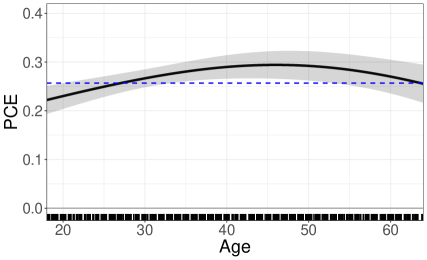
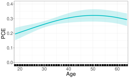
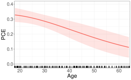
Revisiting the insurance data, the PCE plot for age, along with its associated uncertainty, is shown in Figure 3. It is clear that the covariate effect is significantly different from zero (as previously found in Table 2). The effect for age is positive suggesting that older individuals charge higher expenses to their insurance, on average. Moreover, the effect increases in magnitude as age increases up to about 45 years, then it begins to reduce. Investigating possible interactions, Figure 4 displays the partial covariate effect for age for the two levels of smoker. That the two curves differ suggests the presence of an interaction between the two variables. When smoker is zero (the individual is not a smoker), the effect for age is similar to the one in Figure 3 (and note that most of the individuals are not smokers). However, when smoker is one (the individual is a smoker), the shape of the effect is quite different. The effect is still positive, but it is much higher for younger individuals, i.e., young smokers accrue higher expenses. Furthermore, the PCE decreases with age suggesting that older smokers charge expenses to a lesser extent.

5 Simulation Study

The simulation study aims to determine the performance of both the single-parameter and the multiple-parameter Wald test for FNNs (described in Section 3). The response is generated from an FNN with known “true” architecture with $p=6$ input nodes, where $x_{1},x_{2},\ldots,x_{6}$ are generated from a standard normal distribution. The ratio of non-zero-to-zero covariates (N-Z) is varied (a zero covariate has $\omega_{j}=0_{q}$) to allow for ratios of 5-to-1 (denoted 5-1), and 1-to-1 (denoted 3-3). More specifically, in the 5-1 scenario, $x_{1}$ is the zero covariate; and in the 3-3 scenario, $x_{1},x_{3},x_{4}$ are the zero covariates. (The specific parameter values can be found in Appendix C.) Also, the hidden-layer structure is varied to contain $q\in\{2,4,6\}$ hidden nodes. This allows for a number of different architectures to be explored, and, in particular, cases where the number of non-zero covariates is less than and greater than the number of hidden nodes. Sample sizes of size 500, 1000 and 2000 are investigated, and each scenario is repeated for 1000 replicates. Due to the presence of local maxima in the parameter space, and the requirement for initial weights to begin neural network learning, each model is allowed ten random initialisations to improve its chances of finding a global solution.

Table 3 contains the results from both the single-parameter and multiple-parameter Wald tests. For each scenario of the single-parameter test, the empirical type-I error for a significance test with $\alpha=0.05$ for the true-zero parameter $\omega_{11}$ (Type-I) and the empirical power of the significance test for the non-zero parameter $\omega_{21}$ (Power) are reported. Similarly, for the multiple-parameter test, the empirical type-I error for a significance test with $\alpha=0.05$ for the true-zero covariate $x_{1}$, via $\omega_{1}$, (Type-I), and the empirical power of the significance test for the non-zero covariate $x_{2}$, via $\omega_{2}$, (Power) are reported. In order to determine the performance of the single-parameter test, the symmetries in the weight space need to be considered. Therefore, for each replicate, $\hat{\theta}$ is compared to the true $\theta$ vector, and the necessary node reshuffling and sign flipping is performed to make each $\hat{\theta}$ comparable across simulation replicates (see Appendix A for more information on symmetries in the weight space). As mentioned earlier, issues of parameter redundancy and non-identifiability can arise when fitting these models, leading to issues in computing $\hat{\Sigma}$. We have investigated this issue in a preliminary simulation study, the results of which (provided in Appendix B) highlight the importance of including the ridge penalty; this is included in all numerical studies presented in the main paper where we fix $\lambda=0.01$.

Table 3: Simulation: estimates of rejection rates for both the single-parameter and multiple-parameter Wald tests.

			Single Parameter						Multiple Parameter
			$n=500$		$n=1000$		$n=2000$		$n=500$		$n=1000$		$n=2000$
$q$	N-Z	$K^{*}$	Type-I	Power	Type-I	Power	Type-I	Power	Type-I	Power	Type-I	Power	Type-I	Power
2	5-1	15	0.058	0.596	0.066	0.687	0.068	0.818	0.050	0.999	0.054	1.000	0.053	1.000
	3-3	11	0.068	0.650	0.044	0.747	0.041	0.889	0.055	1.000	0.039	1.000	0.042	1.000
4	5-1	29	0.054	0.535	0.054	0.767	0.061	0.835	0.038	0.767	0.048	1.000	0.057	1.000
	3-3	21	0.055	0.619	0.046	0.806	0.060	0.925	0.035	0.851	0.035	0.996	0.037	1.000
6	5-1	43	0.056	0.502	0.053	0.762	0.054	0.859	0.053	0.990	0.064	1.000	0.035	1.000
	3-3	31	0.194	0.433	0.147	0.547	0.128	0.749	0.489	0.979	0.320	0.998	0.299	1.000
$n$, sample size; $q$, number of nodes in the hidden layer; N-Z, ratio of non-zero-to-zero covariates; $K^{*}$, number of non-zero parameters in the neural network; Type-I, type-I error for $\omega_{11}$ for the single-parameter test and type-I error for $\omega_{1}$ for the multiple-parameter test; Power, statistical power for $\omega_{21}$ for the single-parameter test and statistical power for $\omega_{2}$ for the multiple-parameter test.

For both the single- and multiple-parameter Wald tests, when the number of non-zero covariates (N) is greater than the number of hidden nodes ($N>q$), the test performs well both in terms of type-I error and statistical power. However, when the number of non-zero covariates is less than the number of hidden nodes ($N<q$), neither test performs well in terms of the type-I error (albeit the multiple-parameter test still appears to be powerful). This highlights the importance of the neural network architecture, and indicates a clear trade-off between model flexibility and the ability to perform statistical inference. Here, we have focused on $\omega_{11}$, $\omega_{21}$, $x_{1}$ via $\omega_{1}$, and $x_{2}$ via $\omega_{2}$, but the results are similar for the other parameters and covariates, and these results can be found in the Appendix C.

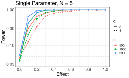
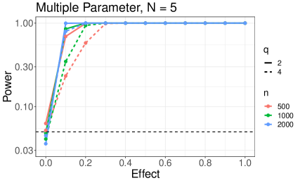
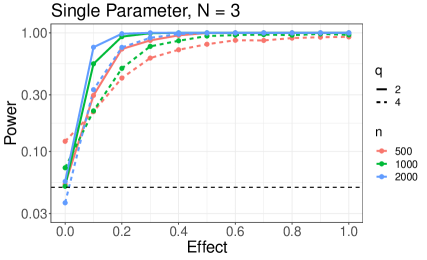
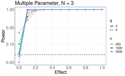
To further investigate the performance of the Wald tests and, in particular, the statistical power for increasing effect sizes, we varied the effect of covariate $x_{2}$ by varying the values of $\omega_{2}=(\omega_{21},\dotsc,\omega_{2q})^{T}$ such that each $\omega_{2k}$ has the same weight value for values $0,0.1,0.2,\dotsc,1.0$ (i.e., in the first scenario $\omega_{2}=(0,\dotsc,0)^{T}$, in the second scenario $\omega_{2}=(0.1,\dotsc,0.1)^{T}$ and so on). This ensures that weights do not oppose each other (e.g., a positive weight cancelling with a negative weight) and the effect grows at a similar rate between each scenario. Figure 5 contains a plot of the power versus effect size (the value of $\omega_{2k}$) for both the single- and multiple-parameter tests (the single-parameter test is evaluated using $\omega_{21}$); results are shown for the number of hidden nodes $q\in\{2,4\}$. The tests perform as expected: the power (i) is approximately at the nominal significance level ($\alpha=0.05$) when there is no effect, except when $N<q$ and $n$ is relatively small (as per Table 3), (ii) approaches one as the effect size increases, and (iii) converges to one more quickly in larger samples and more slowly in more complex models (larger $q$). It is important to note that the power of the multiple-parameter Wald test increases far more quickly than for the single-parameter test. In other words, it is easier to detect an overall covariate effect (which is the combination of multiple weights) than it is to detect the effect of one specific weight; indeed, the former will typically be of greater interest in practice.

Figure 5: Plot of the statistical power (on a logarithmic scale) for the single- and multiple-parameter Wald test as the size of the effect varies for different sample sizes for $N=5$ (top) and $N=3$ (bottom).

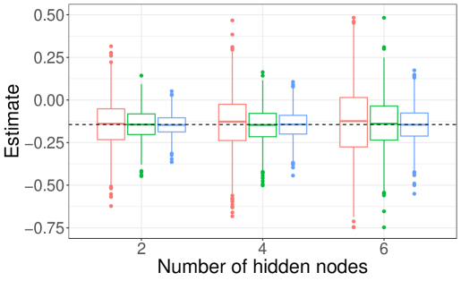
For the 5-1 scenario, additional estimation and inferential performance metrics are examined in Table 4. More specifically, we display the average estimate over simulation replicates ($\hat{\theta}$), the true standard error (SE) (i.e., the standard deviation of the estimates over the replicates), the average estimated standard error (SEE) (computed using Equation 2.4 in a given replicate), and the empirical coverage probability (CP) for a nominal 95% confidence interval. In the interest of brevity, only the results for one input-to-hidden-layer weight vector, $\omega_{2}$, are displayed. (The results for all parameters are available in Appendix C.) Boxplots of the estimates for $\omega_{21}$ for each value of $n$ and $q$ are displayed in Figure 6. We find that estimation bias is relatively low, uncertainty quantification is acceptable in the sense that the SEs are well estimated by the SEEs and the confidence interval coverage is near the nominal 95% level; moreover, the estimation performance and uncertainty quantification improve with the sample size as expected. The results from the 3-3 scenario can be found in Appendix C. As expected from our earlier results, the performance is good when $N=3$ with $q=2$ (more non-zero covariates than hidden nodes); it is slightly poorer but still acceptable when $N=3$ with $q=4$ (similar number of non-zero covariates and hidden nodes); and it is unacceptable when $N=3$ and $q=6$ (fewer non-zero covariates than hidden nodes).

Table 4: Simulation: estimation and inference metrics for the 5-1 non-zero-to-zero (N-Z) scenario.

N-Z	5-1		$n=500$				$n=1000$				$n=2000$
$q$		$\theta$	$\hat{\theta}$	SE	SEE	CP	$\hat{\theta}$	SE	SEE	CP	$\hat{\theta}$	SE	SEE	CP
2	$\omega_{21}$	-0.14	-0.14	0.14	0.13	0.95	-0.14	0.09	0.09	0.95	-0.15	0.06	0.06	0.94
	$\omega_{22}$	-0.27	-0.27	0.06	0.06	0.95	-0.27	0.04	0.04	0.94	-0.27	0.03	0.03	0.95
4	$\omega_{21}$	-0.14	-0.14	0.17	0.17	0.95	-0.15	0.10	0.10	0.95	-0.15	0.09	0.08	0.95
	$\omega_{22}$	-0.27	-0.28	0.11	0.10	0.94	-0.27	0.06	0.06	0.95	-0.27	0.05	0.04	0.94
	$\omega_{23}$	-0.20	-0.22	0.14	0.12	0.95	-0.21	0.08	0.08	0.95	-0.20	0.06	0.06	0.93
	$\omega_{24}$	-0.29	-0.30	0.12	0.11	0.96	-0.29	0.07	0.07	0.94	-0.29	0.05	0.05	0.95
6	$\omega_{21}$	-0.14	-0.14	0.24	0.20	0.93	-0.14	0.15	0.14	0.94	-0.15	0.10	0.10	0.95
	$\omega_{22}$	-0.27	-0.28	0.14	0.12	0.93	-0.28	0.09	0.08	0.94	-0.27	0.05	0.06	0.94
	$\omega_{23}$	-0.20	-0.22	0.19	0.15	0.92	-0.21	0.11	0.10	0.93	-0.20	0.07	0.07	0.95
	$\omega_{24}$	-0.29	-0.30	0.13	0.12	0.92	-0.30	0.09	0.08	0.94	-0.29	0.06	0.06	0.95
	$\omega_{25}$	0.27	0.26	0.11	0.10	0.91	0.27	0.07	0.06	0.94	0.27	0.05	0.04	0.95
	$\omega_{26}$	0.20	0.20	0.09	0.08	0.91	0.20	0.06	0.06	0.93	0.20	0.04	0.04	0.94
Full results for all parameters available in Appendix C; SE, standard deviation of estimates over 1000 replications; SEE, average of estimated standard errors over 1000 replications; CP, the empirical coverage probability of a nominal 95% confidence interval.

Figure 6: Boxplots for $\hat{\omega}_{21}$ for different values of $n$ and $q$. Dashed line denotes the true value ($\omega_{21}=-0.14$).

6 Application to Data

The application to the insurance data, which has been revisited throughout the paper, is now explored in more detail. There are 1,338 observations in total, and the explanatory variables are: the age of the primary beneficiary (age), their gender (sex), their body mass index (bmi), the number of dependents covered by the insurance plan (children), an indicator of the insured’s smoking status (smoker), and their region of residence (region), which is divided into north-east (region.ne), south-east (region.se), south-west (region.sw), and north-west (region.nw). The response variable is the total medical expenses charged to the plan for the calendar year in $1000s of dollars (charges). All numeric covariates are standardised to have zero mean and unit variance, and all categorical covariates are dummy encoded. The variables that are dummy encoded are named variable.level to clarify which level of the variable is represented by a dummy value of one (e.g. sex.male). The response variable is also standardised to have zero mean and unit variance. Note that standardisation (of continuous covariates and the response) is done for the purpose of optimisation stability. However, when producing the PCE plots, we transform both back to their original scales.

Figure 7: Cross-validated RMSE $\pm$ one standard error (left) and BIC (right) for a normal linear regression model (represented by number of hidden nodes equal to zero) and neural networks with varying hidden layer size fit to the insurance data.

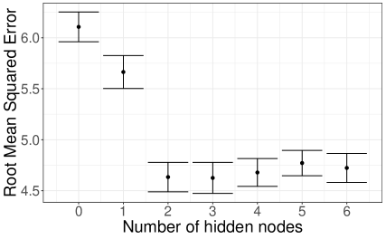
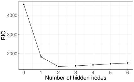
While model selection is not the focus of this paper, in order to apply the proposed statistical-modelling approach for neural networks, the choice of the number of hidden nodes, $q$, is required. Here, we select $q$ by considering both out-of-sample performance using five-fold cross-validation and the Bayesian Information Criterion (BIC). Figure 7 displays the average cross-validated root mean squared error (RMSE) $\pm$ one standard error and the BIC for a normal linear regression model and neural networks with varying hidden layer size, with $\lambda$ set to 0.01 for all neural networks. Based on the out-of-sample predictive performance of the models, it is clear that the additional flexibility of neural networks improves upon the linear model. However, there is no further improvement in performance once the hidden layer size goes beyond two hidden nodes. This is also in agreement with the BIC for each model (fit to the full data set), which obtains a minimum at two hidden nodes.

To further investigate the effect of hidden layer size, the results from the Wald tests for values of $q$ between two and five are visualised in Figure 8. In each model, bmi, children and smoker are found to be statistically significant for the multiple-parameter test at the 5% significance level, while age is significant in all models except when $q=4$. Although we do not test the significance of hidden nodes directly, it is interesting to note that there is no model with more than three hidden nodes that are significant based on the associated single-parameter tests (either all weights entering the node are non-significant or the weight leaving the node is non-significant). This indicates possible redundancy, and supports the findings of Figure 7 that a simpler neural network is sufficient here (albeit, there, a model with $q=2$ is suggested based on the RMSE and BIC). It also further highlights the importance of model selection, as it can be misleading to carry out significance testing on input weights that connect to a hidden node that itself is non-significant. Note that statistically-motivated neural network selection has been considered in McInerney and Burke, (2022).

Figure 8: Results of the single- and multiple-parameter Wald tests overlaid on the neural network architecture for the insurance data for various hidden layer sizes, where $q$ denotes the number of hidden nodes.

Figure 9: PCE plots for bmi (left), children (right), and the binary covariates in the insurance data (bottom). The blue dashed lines/crosses denote the corresponding effects from the linear model in Table 1. The bmi plot is coloured based on the typical categories: underweight, normal, overweight, obesity class I, obesity class II and obesity class III.

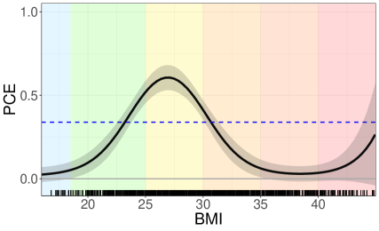
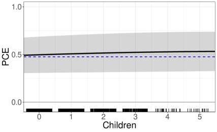
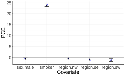
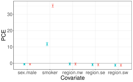
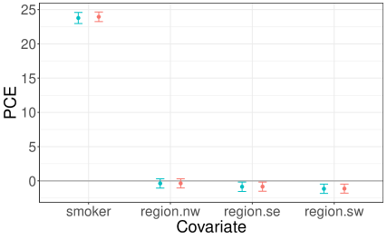
Looking at covariate effects, Figure 9 contains the PCE plots with their 95% confidence intervals for the covariates in the $q=2$ model (the PCE plot for age was displayed earlier in Figure 3). For bmi, the PCE suggests that increased bmi in the range 20 to 35 leads to increased charges. The plot has been overlaid with the colours representing the ranges of the different BMI categories (Centers for Disease Control and Prevention,, 2022). Interestingly, the effect is only present (in varying strength) for individuals who are currently classified as having a BMI that is normal, overweight, or obese class I. An increase in bmi has no effect on charges for individuals classed as underweight, or in obesity class II or III. In other words, underweight individuals are similar to those in the lower range of normal, and obesity classes II and III are similar to those in the upper range of obesity class I. The coefficient for bmi from the linear model is overlaid in the PCE plot. It is clear that the effect found by the neural network is highly non-linear, and the linear model yields an effect that somewhat averages the non-linear effect over the different BMI values. The covariate effect for children is positive, significantly different from zero and appears to be constant, suggesting a linear relationship with charges. For the binary covariates, the strong effect of smoking status is clear, with a PCE of 23.85 associated with smokers compared to non-smokers (i.e., an increase of $23,850 in their medical charges). The other effects are much weaker, and closely align with the results from the multiple-parameter test in Table 2, with region.sw having a non-zero negative effect on charges. Additionally, the PCEs for children and for the binary covariates are very similar to the effects found in the linear model, indicated as blue dashed lines and crosses in Figure 9. Due to the nature of binary covariates (i.e., two-point covariates), the alignment of their PCE values and their corresponding effects from the linear model is to be expected. However, the neural network additionally captures interactions between covariates, which we can also visualise. Figure 10 explores possible interactions between a continuous covariates (bmi) and the binary covariates, and possible interactions between a binary covariate (sex) and the remaining binary covariates. For bmi, there is a clear interaction with smoker; the effect of smoking on charges is much stronger for individuals with a higher BMI value. In contrast, there does not appear to be any interaction between sex and the other binary covariates.

Figure 10: PCE plots investigating possible interaction effects between the binary covariates in the insurance data and bmi (left; set to its mean $\pm$ one standard deviation) and sex (right; set to its two levels).

7 Discussion

The statistical approach to neural networks that we propose illustrates how these models can be made more interpretable and useful for the statistician. Through an application to insurance data, we have demonstrated how a neural network can be used not only as a predictive model, but also as an inferential one. This leads to statistically-based outputs that are more familiar in the statistical modelling context, namely, significance tests and estimated covariate effects. This is critical to ensure the model is intelligible, so that it can be used to provide relevant explanations.

Through extensive simulation studies, we have explored the inferential performance of both single- and multiple-parameter Wald tests in the neural network context, and highlight the circumstances where they perform as expected. This leads to practical recommendations for the neural network architecture when taking a statistical-modelling perspective. We find that the ability to estimate uncertainty comes at a direct trade-off with model flexibility. We recommend that (i) the hidden layer should not be larger than the input layer and (ii) a small ridge penalty should be used to make the estimation more stable. Of course, this raises the issue of model selection for the neural networks, something we have previously explored in McInerney and Burke, (2022), and, moreover, post-selection inference is also worthy of further investigation. We have used a ridge penalty for the purpose of estimation stability only, but it could be varied and selected through cross-validation or an information criterion. Alternatively, a LASSO penalty could be used, which would allow for variable selection, as could modern smooth information-criterion-based penalties such as that of O’Neill and Burke, (2023). These are objectives of our future work.

To accompany the statistical tests, we have proposed covariate-effect plots that mimic regression coefficients. These plots visualise the effect of a $d$-unit increase in the covariate on the response, and they also allow for the detection of possible interaction effects, which, in the future, could also be complimented with more formal statistical testing. Our statistical perspective on neural networks could be extended to models with multiple hidden layers, which are popular in the computer science and machine learning domains. However, it is important to note that even simpler single-hidden-layer neural networks are underutilised in the statistical community despite the fact that they extend more familiar (linear-type) models. We believe that our work (available within the interpretnn R package (McInerney and Burke,, 2023)) makes neural networks more accessible within the broader statistical-modelling context, and can increase their utility to complement the current statistical toolbox.

Appendix A Practical Issues of FNNs

There are some practical considerations that arise when fitting neural networks. Two models may appear different upon initial inspection, but may, in fact, be the same model. In particular, we consider model reducibility and weight uniqueness below, which may mask two equivalent models.

A.1 Reducibilty

An FNN is said to be reducible if its input-to-output mapping is equivalent to another FNN that has fewer hidden nodes (Sussmann,, 1992). If an FNN is reducible, then at least one of the hidden nodes is redundant (i.e., it provides no contribution in the prediction of the response). There are three conditions that, if any are true, result in a reducible FNN:

• One of the $\gamma_{k}$ output weights, for $k=1,...,q$, equals zero. ($\exists~{}k\in\{1,2,\dotsc,q\}\text{~{}s.t.~{}}\gamma_{k}=0$.)

• The net input, $s_{k}(x_{i})=\sum_{j=0}^{p}\omega_{jk}x_{ij}$, for two hidden nodes, $k_{1},k_{2}\in\{1,2,...,q\}$, are sign-equivalent. ($\exists~{}k_{1},k_{2}\in\{1,2,\dotsc,q\}\text{~{}s.t.~{}}\forall i\in 1,\dotsc n,~{}|s_{k_{1}}(x_{i})|=|s_{k_{2}}(x_{i})|$.)

• A hidden node has a net input that is constant. ($\exists~{}k\in\{1,2,\dotsc,q\}\text{~{}s.t.~{}}\forall i\in 1,\dotsc n,~{}s_{k}(x_{i})=c$.)

Redundant hidden nodes can lead to issues of non-identifiability for some of the parameters. An FNN that does not contain any redundant hidden nodes is called irreducible.

A.2 Uniqueness

If an FNN is irreducible, Sussmann, (1992) showed that the neural network weights are unique, up to a finite group of symmetries. A weight vector, $\tilde{\theta}$, is a symmetry of $\theta$ if one of the following is true (assuming a sigmoid activation on the hidden nodes):

• $\tilde{\omega}_{k}=-\omega_{k}$, $\tilde{\gamma}_{k}=-\gamma_{k}$, and $\tilde{\omega}_{0}=\gamma_{0}+\gamma_{k}$, for any $k=1,2,...,q$.

• If the order of the hidden nodes is permuted.

Therefore, $2^{q}(q!)$ symmetries exist, all of which are equivalent and can be considered the global solution.

Appendix B Simulation: Estimation of $\Sigma$

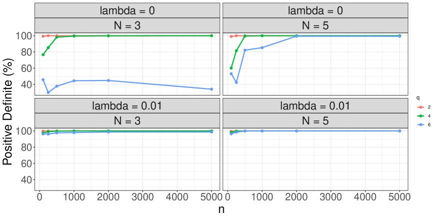
This simulation study aims to determine what conditions are required to ensure a high probability that the estimate of variance-covariance matrix, $\hat{\Sigma}$, is positive definite. The variance-covariance matrix is positive definite if its eigenvalues are all positive real numbers. This is a necessary requirement for any method of uncertainty quantification that uses $\hat{\Sigma}$, such as the Wald hypothesis tests (Section 3), and the delta method. Factors that can affect the positive definiteness of $\hat{\Sigma}$ include parameter redundancy, the architecture (the size of $q$ relative to $p$), the parameter values, the number of parameters relative to the sample size, and the presence or absence of a ridge penalty (commonly used in neural network optimisation).

The simulation setup is similar to the setup of Section 5. However, we have run simulations where there is no ridge penalty ($\lambda=0$) and where there is a small ridge penalty ($\lambda=0.01$) to determine its effect; additional sample sizes are also investigated (100, 250, 500, 1000, 2000 and 5000). For each simulation scenario, the percentage of variance-covariance matrices that are positive definite is reported (PD). The results are summarised in Table 5.

For the scenarios where $\lambda=0$, when the number of non-zero covariates (N) is greater than or equal to the number of hidden nodes ($N\geq q$), and the sample size is relatively large ($n\geq 500$), the percentage of variance-covariance matrices that are positive definite is very high ($\geq 99\%$). However, when there are more hidden nodes than non-zero covariates, the estimation of the variance-covariance matrix is quite unstable, i.e., it cannot be reliably estimated or requires large sample sizes. This is possibly due to the mapping of the input space to a higher-dimensional hidden (latent) space. The addition of a ridge penalty clearly allows for a more stable estimation of $\Sigma$ across the full range of settings considered here. Therefore, we recommend the use of the ridge penalty in practice to stabilise the estimation of the variance-covariance matrix so that statistical inference can at least proceed. Nevertheless, to attain acceptable inferential performance, it is still important not to have an overly complex hidden layer relative to the number of inputs (as shown in Section 5). It is also worth highlighting that the user themselves can assess the positive-definiteness of the information matrix in practice, and seek to simplify the model when this matrix is not positive definite. This justifies the need for neural network model selection methods that focus on producing parsimonious models (McInerney and Burke,, 2022).

Table 5: Simulation: percentage of variance-covariance matrices that are positive definite.

$\lambda$	$q$	N-Z	$n=100$	$n=250$	$n=500$	$n=1000$	$n=2000$	$n=5000$
0	2	5-1	99.1	100.0	100.0	100.0	100.0	100.0
		3-3	99.4	100.0	100.0	100.0	100.0	100.0
	4	5-1	60.1	81.5	99.6	100.0	100.0	100.0
		3-3	76.6	85.3	98.3	99.6	99.9	100.0
	6	5-1	53.2	42.4	82.2	85.3	99.4	99.3
		3-3	45.8	30.0	37.8	44.5	44.8	34.1
0.01	2	5-1	99.6	100.0	100.0	100.0	100.0	100.0
		3-3	99.9	100.0	100.0	100.0	100.0	100.0
	4	5-1	98.3	99.8	100.0	100.0	100.0	100.0
		3-3	97.6	99.1	99.8	100.0	100.0	100.0
	6	5-1	96.4	98.6	99.9	100.0	100.0	100.0
		3-3	96.3	96.2	97.7	98.0	98.7	98.7

Figure 11: Plot of the percentage of variance-covariance matrices that are positive definite for different values of $N$, $q$ and $\lambda$.

Appendix C Estimation and inference metrics

This section contains the full simulation results from Section 5 of the main paper. Tables 6 and 7 contain the rejection rate results for the multiple-parameter Wald test for the 5-1 and 3-3 non-zero-to-zero covariates (N-Z) scenarios, respectively. Tables LABEL:tab:_est_and_inf_5-1 and LABEL:tab:_est_and_inf_3-3 contain the results for the additional estimation and inference metrics, including the rejection rate results for the single-parameter Wald test, for the 5-1 and 3-3 non-zero-to-zero covariates (N-Z) scenarios, respectively.

Table 6: Simulation: estimates of rejection rates for the multiple-parameter Wald test for the 5-1 scenario.

N-Z	5-1	$q=2$			$q=4$			$q=6$
		$n=500$	$n=1000$	$n=2000$	$n=500$	$n=1000$	$n=2000$	$n=500$	$n=1000$	$n=2000$
$\omega_{1}$		0.050	0.054	0.053	0.038	0.048	0.057	0.053	0.064	0.035
$\omega_{2}$		0.999	1.000	1.000	0.767	1.000	1.000	0.990	1.000	1.000
$\omega_{3}$		1.000	1.000	1.000	1.000	1.000	1.000	1.000	1.000	1.000
$\omega_{4}$		1.000	1.000	1.000	1.000	1.000	1.000	1.000	1.000	1.000
$\omega_{5}$		1.000	1.000	1.000	1.000	1.000	1.000	1.000	1.000	1.000
$\omega_{6}$		1.000	1.000	1.000	1.000	1.000	1.000	1.000	1.000	1.000
True zero weight vectors are highlighted in bold.

Table 7: Simulation: estimates of rejection rates for the multiple-parameter Wald test for the 3-3 scenario.

N-Z	3-3	$q=2$			$q=4$			$q=6$
		$n=500$	$n=1000$	$n=2000$	$n=500$	$n=1000$	$n=2000$	$n=500$	$n=1000$	$n=2000$
$\omega_{1}$		0.055	0.039	0.042	0.035	0.035	0.037	0.489	0.320	0.299
$\omega_{2}$		1.000	1.000	1.000	0.851	0.996	1.000	0.979	0.998	1.000
$\omega_{3}$		0.049	0.052	0.055	0.044	0.044	0.037	0.453	0.328	0.365
$\omega_{4}$		0.051	0.040	0.048	0.039	0.039	0.039	0.454	0.350	0.340
$\omega_{5}$		1.000	1.000	1.000	1.000	1.000	1.000	1.000	1.000	1.000
$\omega_{6}$		1.000	1.000	1.000	1.000	1.000	1.000	1.000	1.000	1.000
True zero weight vectors are highlighted in bold.

Table 8: Simulation: estimation and inference metrics for the 5-1 non-zero-to-zero (N-Z) scenario.

N-Z	5-1		$n=500$					$n=1000$					$n=2000$
$q$		$\theta$	$\hat{\theta}$	SE	SEE	CP	RR	$\hat{\theta}$	SE	SEE	CP	RR	$\hat{\theta}$	SE	SEE	CP	RR
2	$\omega_{01}$	-2.77	-2.77	0.43	0.42	0.94	1.00	-2.75	0.29	0.28	0.94	1.00	-2.77	0.20	0.20	0.96	1.00
	$\omega_{11}$	0.00	0.00	0.13	0.12	0.94	0.06	0.00	0.09	0.09	0.93	0.07	0.00	0.06	0.06	0.93	0.07
	$\omega_{21}$	-0.14	-0.14	0.14	0.13	0.95	0.60	-0.14	0.09	0.09	0.95	0.69	-0.15	0.06	0.06	0.94	0.82
	$\omega_{31}$	-0.56	-0.56	0.17	0.17	0.95	0.98	-0.56	0.11	0.11	0.95	1.00	-0.57	0.07	0.07	0.96	1.00
	$\omega_{41}$	2.24	2.24	0.38	0.36	0.93	1.00	2.23	0.25	0.24	0.94	1.00	2.24	0.17	0.17	0.96	1.00
	$\omega_{51}$	-2.52	-2.51	0.41	0.40	0.94	1.00	-2.51	0.28	0.28	0.94	1.00	-2.52	0.19	0.19	0.96	1.00
	$\omega_{61}$	-2.52	-2.52	0.41	0.40	0.94	1.00	-2.51	0.27	0.27	0.93	1.00	-2.52	0.19	0.19	0.95	1.00
	$\omega_{02}$	1.70	1.70	0.14	0.13	0.94	1.00	1.70	0.09	0.09	0.94	1.00	1.70	0.06	0.06	0.94	1.00
	$\omega_{12}$	0.00	0.00	0.05	0.05	0.95	0.05	0.00	0.04	0.04	0.94	0.06	0.00	0.02	0.02	0.95	0.05
	$\omega_{22}$	-0.27	-0.27	0.06	0.06	0.95	0.58	-0.27	0.04	0.04	0.94	0.70	-0.27	0.03	0.03	0.95	0.83
	$\omega_{32}$	0.56	0.56	0.07	0.06	0.95	0.99	0.56	0.05	0.05	0.96	1.00	0.56	0.03	0.03	0.94	1.00
	$\omega_{42}$	1.71	1.71	0.13	0.13	0.95	1.00	1.71	0.09	0.09	0.94	1.00	1.71	0.06	0.07	0.95	1.00
	$\omega_{52}$	1.05	1.06	0.10	0.10	0.94	1.00	1.06	0.07	0.07	0.95	1.00	1.06	0.05	0.05	0.95	1.00
	$\omega_{62}$	-2.06	-2.07	0.16	0.15	0.93	1.00	-2.07	0.12	0.11	0.94	1.00	-2.06	0.07	0.08	0.96	1.00
	$\gamma_{0}$	-1.54	-1.55	0.06	0.07	0.94	0.34	-1.55	0.05	0.05	0.94	0.52	-1.55	0.04	0.04	0.95	0.85
	$\gamma_{1}$	1.37	1.39	0.09	0.09	0.94	1.00	1.38	0.07	0.07	0.95	1.00	1.37	0.04	0.04	0.95	1.00
	$\gamma_{2}$	2.73	2.73	0.10	0.10	0.95	1.00	2.73	0.07	0.07	0.95	1.00	2.73	0.05	0.05	0.96	1.00
4	$\omega_{01}$	-2.77	-2.79	0.50	0.49	0.94	1.00	-2.79	0.32	0.33	0.95	1.00	-2.78	0.25	0.25	0.94	1.00
	$\omega_{11}$	0.00	0.01	0.17	0.16	0.95	0.05	0.00	0.11	0.11	0.95	0.05	0.00	0.08	0.08	0.94	0.06
	$\omega_{21}$	-0.14	-0.14	0.17	0.17	0.95	0.54	-0.15	0.10	0.10	0.95	0.77	-0.15	0.09	0.08	0.95	0.84
	$\omega_{31}$	-0.56	-0.57	0.20	0.19	0.94	0.93	-0.57	0.13	0.12	0.94	0.99	-0.56	0.10	0.10	0.96	1.00
	$\omega_{41}$	2.24	2.26	0.43	0.41	0.94	1.00	2.26	0.28	0.28	0.96	1.00	2.26	0.21	0.21	0.94	1.00
	$\omega_{51}$	-2.52	-2.53	0.49	0.48	0.94	1.00	-2.54	0.33	0.33	0.95	1.00	-2.53	0.26	0.25	0.94	1.00
	$\omega_{61}$	-2.52	-2.55	0.46	0.47	0.95	1.00	-2.54	0.32	0.32	0.95	1.00	-2.53	0.24	0.23	0.94	1.00
	$\omega_{02}$	1.70	1.69	0.32	0.30	0.92	1.00	1.71	0.23	0.21	0.94	1.00	1.71	0.15	0.15	0.94	1.00
	$\omega_{12}$	0.00	0.00	0.09	0.08	0.96	0.04	0.00	0.06	0.06	0.94	0.06	0.00	0.05	0.04	0.95	0.05
	$\omega_{22}$	-0.27	-0.28	0.11	0.10	0.94	0.56	-0.27	0.06	0.06	0.95	0.78	-0.27	0.05	0.04	0.94	0.82
	$\omega_{32}$	0.56	0.56	0.14	0.14	0.95	0.94	0.57	0.11	0.10	0.94	1.00	0.56	0.07	0.07	0.95	1.00
	$\omega_{42}$	1.71	1.70	0.27	0.26	0.93	1.00	1.72	0.19	0.18	0.94	1.00	1.71	0.13	0.12	0.95	1.00
	$\omega_{52}$	1.05	1.06	0.17	0.16	0.95	1.00	1.06	0.12	0.12	0.95	1.00	1.06	0.08	0.08	0.96	1.00
	$\omega_{62}$	-2.06	-2.07	0.31	0.30	0.94	1.00	-2.08	0.22	0.21	0.94	1.00	-2.08	0.14	0.14	0.95	1.00
	$\omega_{03}$	2.08	2.12	0.46	0.45	0.94	1.00	2.10	0.32	0.30	0.94	1.00	2.08	0.22	0.22	0.94	1.00
	$\omega_{13}$	0.00	0.01	0.12	0.11	0.95	0.05	0.00	0.08	0.07	0.94	0.06	0.00	0.05	0.05	0.94	0.06
	$\omega_{23}$	-0.20	-0.22	0.14	0.12	0.95	0.51	-0.21	0.08	0.08	0.95	0.77	-0.20	0.06	0.06	0.93	0.85
	$\omega_{33}$	-0.60	-0.61	0.16	0.15	0.96	0.94	-0.61	0.11	0.11	0.95	1.00	-0.60	0.07	0.07	0.94	1.00
	$\omega_{43}$	-2.89	-2.96	0.51	0.50	0.93	1.00	-2.92	0.36	0.34	0.94	1.00	-2.89	0.25	0.24	0.93	1.00
	$\omega_{53}$	-1.43	-1.49	0.29	0.29	0.94	1.00	-1.44	0.20	0.19	0.94	1.00	-1.43	0.14	0.14	0.94	1.00
	$\omega_{63}$	1.48	1.48	0.29	0.28	0.92	1.00	1.49	0.21	0.19	0.95	1.00	1.48	0.13	0.13	0.94	1.00
	$\omega_{04}$	3.00	3.01	0.40	0.41	0.94	1.00	3.02	0.29	0.29	0.96	1.00	3.01	0.20	0.20	0.96	1.00
	$\omega_{14}$	0.00	0.00	0.10	0.10	0.95	0.05	0.00	0.08	0.07	0.96	0.04	0.00	0.06	0.05	0.94	0.06
	$\omega_{24}$	-0.29	-0.30	0.12	0.11	0.96	0.53	-0.29	0.07	0.07	0.94	0.77	-0.29	0.05	0.05	0.95	0.86
	$\omega_{34}$	-0.42	-0.42	0.15	0.16	0.94	0.93	-0.42	0.11	0.11	0.95	0.99	-0.42	0.07	0.07	0.94	1.00
	$\omega_{44}$	1.40	1.40	0.20	0.20	0.94	1.00	1.41	0.13	0.13	0.95	1.00	1.40	0.10	0.09	0.95	1.00
	$\omega_{54}$	2.86	2.88	0.40	0.43	0.94	1.00	2.89	0.31	0.31	0.95	1.00	2.87	0.20	0.20	0.96	1.00
	$\omega_{64}$	-2.08	-2.09	0.27	0.27	0.93	1.00	-2.09	0.18	0.19	0.94	1.00	-2.08	0.13	0.13	0.95	1.00
	$\gamma_{0}$	-1.54	-1.55	0.27	0.27	0.95	0.14	-1.54	0.20	0.18	0.94	0.24	-1.53	0.14	0.14	0.95	0.22
	$\gamma_{1}$	1.37	1.41	0.13	0.13	0.96	1.00	1.38	0.10	0.09	0.93	1.00	1.38	0.07	0.07	0.94	1.00
	$\gamma_{2}$	2.73	2.84	0.50	0.53	0.94	1.00	2.77	0.40	0.38	0.95	1.00	2.74	0.23	0.23	0.95	1.00
	$\gamma_{3}$	-1.81	-1.81	0.22	0.22	0.94	1.00	-1.82	0.17	0.16	0.94	1.00	-1.82	0.12	0.12	0.95	1.00
	$\gamma_{4}$	-2.56	-2.66	0.45	0.47	0.94	1.00	-2.60	0.35	0.34	0.96	1.00	-2.57	0.20	0.20	0.94	1.00
6	$\omega_{01}$	-2.77	-2.68	1.12	0.84	0.91	0.98	-2.76	0.67	0.60	0.92	1.00	-2.75	0.42	0.42	0.95	1.00
	$\omega_{11}$	0.00	0.02	0.24	0.20	0.94	0.06	0.00	0.14	0.13	0.95	0.05	0.00	0.10	0.10	0.95	0.05
	$\omega_{21}$	-0.14	-0.14	0.24	0.20	0.93	0.50	-0.14	0.15	0.14	0.94	0.76	-0.15	0.10	0.10	0.95	0.86
	$\omega_{31}$	-0.56	-0.56	0.33	0.25	0.92	0.91	-0.57	0.20	0.18	0.93	0.99	-0.57	0.13	0.12	0.95	1.00
	$\omega_{41}$	2.24	2.26	0.68	0.61	0.91	1.00	2.27	0.47	0.44	0.93	1.00	2.24	0.31	0.31	0.96	1.00
	$\omega_{51}$	-2.52	-2.50	0.87	0.69	0.91	1.00	-2.56	0.54	0.49	0.92	1.00	-2.52	0.33	0.34	0.95	1.00
	$\omega_{61}$	-2.52	-2.55	0.75	0.66	0.90	1.00	-2.55	0.50	0.47	0.94	1.00	-2.52	0.33	0.33	0.95	1.00
	$\omega_{02}$	1.70	1.75	0.58	0.36	0.91	0.97	1.72	0.28	0.24	0.92	1.00	1.71	0.17	0.16	0.94	1.00
	$\omega_{12}$	0.00	0.00	0.14	0.11	0.94	0.06	0.00	0.07	0.07	0.93	0.07	0.00	0.05	0.05	0.96	0.04
	$\omega_{22}$	-0.27	-0.28	0.14	0.12	0.93	0.54	-0.28	0.09	0.08	0.94	0.78	-0.27	0.05	0.06	0.94	0.88
	$\omega_{32}$	0.56	0.57	0.23	0.17	0.90	0.92	0.57	0.13	0.13	0.94	0.99	0.56	0.09	0.08	0.94	1.00
	$\omega_{42}$	1.71	1.75	0.43	0.31	0.91	1.00	1.73	0.27	0.22	0.93	1.00	1.72	0.15	0.15	0.93	1.00
	$\omega_{52}$	1.05	1.04	0.39	0.22	0.91	1.00	1.07	0.16	0.15	0.93	1.00	1.06	0.10	0.10	0.94	1.00
	$\omega_{62}$	-2.06	-2.14	0.46	0.36	0.93	1.00	-2.11	0.29	0.25	0.93	1.00	-2.08	0.17	0.17	0.95	1.00
	$\omega_{03}$	2.08	2.14	0.63	0.52	0.91	0.98	2.09	0.41	0.34	0.94	1.00	2.09	0.23	0.24	0.95	1.00
	$\omega_{13}$	0.00	0.01	0.17	0.13	0.95	0.05	-0.01	0.10	0.09	0.94	0.06	0.00	0.06	0.06	0.95	0.05
	$\omega_{23}$	-0.20	-0.22	0.19	0.15	0.92	0.54	-0.21	0.11	0.10	0.93	0.75	-0.20	0.07	0.07	0.95	0.87
	$\omega_{33}$	-0.60	-0.62	0.23	0.18	0.90	0.90	-0.59	0.14	0.13	0.95	0.99	-0.60	0.09	0.09	0.94	1.00
	$\omega_{43}$	-2.89	-2.97	0.84	0.60	0.91	1.00	-2.91	0.52	0.39	0.94	1.00	-2.91	0.26	0.27	0.94	1.00
	$\omega_{53}$	-1.43	-1.48	0.48	0.33	0.92	1.00	-1.43	0.32	0.22	0.93	1.00	-1.44	0.15	0.15	0.94	1.00
	$\omega_{63}$	1.48	1.49	0.62	0.34	0.90	1.00	1.47	0.33	0.22	0.94	1.00	1.49	0.15	0.15	0.94	1.00
	$\omega_{04}$	3.00	3.08	0.54	0.47	0.88	0.98	3.02	0.36	0.34	0.94	1.00	3.00	0.24	0.23	0.95	1.00
	$\omega_{14}$	0.00	0.00	0.13	0.12	0.95	0.05	0.00	0.08	0.07	0.94	0.06	0.00	0.06	0.06	0.96	0.04
	$\omega_{24}$	-0.29	-0.30	0.13	0.12	0.92	0.53	-0.30	0.09	0.08	0.94	0.77	-0.29	0.06	0.06	0.95	0.88
	$\omega_{34}$	-0.42	-0.43	0.18	0.15	0.91	0.92	-0.43	0.13	0.12	0.94	0.99	-0.42	0.08	0.09	0.94	1.00
	$\omega_{44}$	1.40	1.43	0.27	0.21	0.90	1.00	1.40	0.16	0.15	0.94	1.00	1.40	0.11	0.10	0.94	1.00
	$\omega_{54}$	2.86	2.93	0.57	0.48	0.90	1.00	2.88	0.41	0.35	0.94	1.00	2.87	0.26	0.25	0.94	1.00
	$\omega_{64}$	-2.08	-2.13	0.39	0.33	0.90	1.00	-2.10	0.22	0.21	0.93	1.00	-2.08	0.16	0.15	0.94	1.00
	$\omega_{05}$	2.79	2.69	0.46	0.40	0.92	0.99	2.74	0.30	0.28	0.94	1.00	2.77	0.20	0.20	0.94	1.00
	$\omega_{15}$	0.00	0.00	0.09	0.08	0.94	0.06	0.00	0.07	0.06	0.95	0.05	0.00	0.04	0.04	0.96	0.04
	$\omega_{25}$	0.27	0.26	0.11	0.10	0.91	0.55	0.27	0.07	0.06	0.94	0.77	0.27	0.05	0.04	0.95	0.85
	$\omega_{35}$	-0.56	-0.54	0.11	0.10	0.93	0.92	-0.55	0.08	0.08	0.94	0.99	-0.55	0.05	0.05	0.94	1.00
	$\omega_{45}$	2.03	1.99	0.28	0.26	0.91	1.00	2.02	0.19	0.18	0.93	1.00	2.02	0.13	0.12	0.94	1.00
	$\omega_{55}$	-2.83	-2.76	0.41	0.36	0.90	1.00	-2.80	0.27	0.25	0.94	1.00	-2.82	0.18	0.17	0.94	1.00
	$\omega_{65}$	-1.93	-1.90	0.27	0.25	0.92	1.00	-1.91	0.18	0.16	0.94	1.00	-1.92	0.12	0.12	0.94	1.00
	$\omega_{06}$	-1.82	-1.85	0.21	0.19	0.91	0.97	-1.83	0.14	0.13	0.93	1.00	-1.82	0.09	0.09	0.95	1.00
	$\omega_{16}$	0.00	0.00	0.09	0.08	0.94	0.06	0.00	0.05	0.05	0.94	0.06	0.00	0.04	0.04	0.94	0.06
	$\omega_{26}$	0.20	0.20	0.09	0.08	0.91	0.52	0.20	0.06	0.06	0.93	0.75	0.20	0.04	0.04	0.94	0.86
	$\omega_{36}$	-0.39	-0.41	0.09	0.09	0.91	0.91	-0.39	0.06	0.06	0.92	0.98	-0.39	0.04	0.04	0.97	1.00
	$\omega_{46}$	-1.92	-1.95	0.25	0.23	0.92	1.00	-1.94	0.15	0.15	0.93	1.00	-1.92	0.11	0.10	0.95	1.00
	$\omega_{56}$	-2.78	-2.83	0.30	0.28	0.91	1.00	-2.80	0.20	0.19	0.94	1.00	-2.79	0.13	0.13	0.95	1.00
	$\omega_{66}$	-2.38	-2.42	0.28	0.26	0.91	1.00	-2.40	0.17	0.17	0.94	1.00	-2.39	0.12	0.12	0.94	1.00
	$\gamma_{0}$	-1.54	-1.50	0.44	0.35	0.92	0.38	-1.52	0.28	0.23	0.94	0.49	-1.53	0.16	0.16	0.96	0.37
	$\gamma_{1}$	1.37	1.57	0.49	0.33	0.92	1.00	1.44	0.23	0.19	0.94	1.00	1.40	0.13	0.13	0.96	1.00
	$\gamma_{2}$	2.73	2.83	0.66	0.58	0.93	1.00	2.80	0.59	0.45	0.94	1.00	2.77	0.32	0.31	0.95	1.00
	$\gamma_{3}$	-1.81	-1.82	0.49	0.28	0.93	1.00	-1.83	0.22	0.19	0.94	1.00	-1.82	0.13	0.13	0.94	1.00
	$\gamma_{4}$	-2.56	-2.67	0.54	0.49	0.93	1.00	-2.62	0.39	0.39	0.93	1.00	-2.60	0.28	0.27	0.94	1.00
	$\gamma_{5}$	-2.87	-3.08	0.49	0.33	0.93	1.00	-2.94	0.20	0.18	0.95	1.00	-2.91	0.11	0.11	0.95	1.00
	$\gamma_{6}$	2.98	2.98	0.23	0.21	0.93	1.00	2.98	0.14	0.13	0.94	1.00	2.98	0.10	0.09	0.95	1.00
SE, standard deviation of estimates over 1000 replications; SEE, average of estimated standard errors over 1000 replications; CP, the empirical coverage probability of a nominal 95% confidence interval; RR, the rejection rate for the single-parameter Wald test with a 5% significance level. True zero parameters are highlighted in bold.

Table 9: Simulation: estimation and inference metrics for the 3-3 non-zero-to-zero (N-Z) scenario.

N-Z	3-3		$n=500$					$n=1000$					$n=2000$
$q$		$\theta$	$\hat{\theta}$	SE	SEE	CP	RR	$\hat{\theta}$	SE	SEE	CP	RR	$\hat{\theta}$	SE	SEE	CP	RR
2	$\omega_{01}$	-2.77	-2.75	0.35	0.34	0.94	1.00	-2.76	0.25	0.24	0.94	1.00	-2.76	0.17	0.18	0.96	1.00
	$\omega_{11}$	0.00	0.00	0.11	0.10	0.93	0.07	0.00	0.07	0.07	0.96	0.04	0.00	0.05	0.05	0.96	0.04
	$\omega_{21}$	-0.14	-0.14	0.11	0.10	0.94	0.65	-0.14	0.07	0.07	0.95	0.75	-0.14	0.05	0.05	0.95	0.89
	$\omega_{31}$	0.00	-0.01	0.11	0.10	0.94	0.06	0.00	0.07	0.07	0.95	0.05	0.00	0.05	0.05	0.95	0.05
	$\omega_{41}$	0.00	0.00	0.10	0.10	0.94	0.06	0.00	0.07	0.07	0.96	0.04	0.00	0.05	0.05	0.96	0.04
	$\omega_{51}$	-2.52	-2.49	0.35	0.35	0.94	1.00	-2.51	0.24	0.24	0.95	1.00	-2.51	0.17	0.17	0.95	1.00
	$\omega_{61}$	-2.52	-2.50	0.36	0.37	0.94	1.00	-2.51	0.25	0.25	0.94	1.00	-2.52	0.17	0.18	0.95	1.00
	$\omega_{02}$	1.70	1.70	0.11	0.11	0.94	1.00	1.70	0.08	0.08	0.94	1.00	1.70	0.06	0.06	0.94	1.00
	$\omega_{12}$	0.00	0.00	0.04	0.04	0.95	0.05	0.00	0.03	0.03	0.95	0.05	0.00	0.02	0.02	0.95	0.05
	$\omega_{22}$	-0.27	-0.27	0.04	0.04	0.95	0.65	-0.27	0.03	0.03	0.94	0.76	-0.27	0.02	0.02	0.95	0.89
	$\omega_{32}$	0.00	0.00	0.04	0.04	0.95	0.05	0.00	0.03	0.03	0.95	0.05	0.00	0.02	0.02	0.96	0.04
	$\omega_{42}$	0.00	0.00	0.04	0.04	0.96	0.04	0.00	0.03	0.03	0.96	0.04	0.00	0.02	0.02	0.95	0.05
	$\omega_{52}$	1.05	1.07	0.09	0.09	0.94	1.00	1.06	0.06	0.06	0.93	1.00	1.06	0.04	0.04	0.95	1.00
	$\omega_{62}$	-2.06	-2.08	0.16	0.15	0.94	1.00	-2.06	0.10	0.10	0.94	1.00	-2.06	0.08	0.07	0.95	1.00
	$\gamma_{0}$	-1.54	-1.54	0.10	0.09	0.94	0.22	-1.55	0.06	0.06	0.95	0.55	-1.55	0.04	0.04	0.95	0.83
	$\gamma_{1}$	1.37	1.39	0.10	0.10	0.96	1.00	1.38	0.06	0.06	0.94	1.00	1.38	0.05	0.05	0.95	1.00
	$\gamma_{2}$	2.73	2.72	0.13	0.12	0.94	1.00	2.73	0.08	0.08	0.94	1.00	2.73	0.06	0.06	0.95	1.00
4	$\omega_{01}$	-2.77	-2.73	0.38	0.37	0.92	0.96	-2.74	0.29	0.28	0.93	1.00	-2.76	0.21	0.20	0.96	1.00
	$\omega_{11}$	0.00	0.00	0.12	0.12	0.94	0.06	0.00	0.08	0.08	0.95	0.05	0.00	0.06	0.06	0.94	0.06
	$\omega_{21}$	-0.14	-0.14	0.12	0.12	0.93	0.62	-0.14	0.09	0.09	0.94	0.81	-0.14	0.06	0.06	0.95	0.92
	$\omega_{31}$	0.00	0.00	0.12	0.11	0.95	0.05	0.00	0.08	0.08	0.96	0.04	0.00	0.06	0.06	0.95	0.05
	$\omega_{41}$	0.00	0.00	0.12	0.11	0.95	0.05	0.00	0.09	0.08	0.96	0.04	0.00	0.06	0.06	0.95	0.05
	$\omega_{51}$	-2.52	-2.45	0.38	0.37	0.93	1.00	-2.48	0.28	0.28	0.94	1.00	-2.51	0.20	0.20	0.95	1.00
	$\omega_{61}$	-2.52	-2.48	0.39	0.39	0.92	1.00	-2.50	0.29	0.29	0.94	1.00	-2.52	0.20	0.20	0.95	1.00
	$\omega_{02}$	1.70	1.71	0.37	0.27	0.91	0.97	1.73	0.21	0.19	0.94	1.00	1.72	0.13	0.13	0.96	1.00
	$\omega_{12}$	0.00	0.01	0.08	0.08	0.96	0.04	0.00	0.06	0.06	0.95	0.05	0.00	0.04	0.04	0.95	0.05
	$\omega_{22}$	-0.27	-0.30	0.11	0.10	0.94	0.61	-0.29	0.07	0.07	0.94	0.82	-0.28	0.05	0.05	0.95	0.93
	$\omega_{32}$	0.00	0.00	0.08	0.07	0.95	0.05	0.00	0.05	0.05	0.96	0.04	0.00	0.04	0.04	0.94	0.06
	$\omega_{42}$	0.00	-0.01	0.08	0.08	0.95	0.05	0.00	0.05	0.06	0.95	0.05	0.00	0.04	0.04	0.95	0.05
	$\omega_{52}$	1.05	1.05	0.20	0.18	0.92	1.00	1.05	0.14	0.14	0.95	1.00	1.05	0.10	0.10	0.95	1.00
	$\omega_{62}$	-2.06	-2.11	0.36	0.30	0.93	1.00	-2.11	0.22	0.21	0.96	1.00	-2.09	0.15	0.15	0.95	1.00
	$\omega_{03}$	2.08	1.96	0.63	0.58	0.93	0.98	2.01	0.46	0.43	0.94	1.00	2.05	0.29	0.30	0.95	1.00
	$\omega_{13}$	0.00	0.01	0.08	0.08	0.96	0.04	0.00	0.05	0.05	0.94	0.06	0.00	0.04	0.03	0.95	0.05
	$\omega_{23}$	-0.20	-0.21	0.11	0.10	0.93	0.61	-0.20	0.08	0.07	0.94	0.81	-0.20	0.05	0.05	0.94	0.91
	$\omega_{33}$	0.00	0.00	0.08	0.07	0.95	0.05	0.00	0.05	0.05	0.95	0.05	0.00	0.04	0.04	0.94	0.06
	$\omega_{43}$	0.00	0.00	0.08	0.07	0.96	0.04	0.00	0.05	0.05	0.95	0.05	0.00	0.03	0.03	0.94	0.06
	$\omega_{53}$	-1.43	-1.38	0.49	0.34	0.94	1.00	-1.41	0.31	0.25	0.94	1.00	-1.42	0.17	0.17	0.96	1.00
	$\omega_{63}$	1.48	1.35	0.60	0.35	0.93	1.00	1.44	0.34	0.26	0.95	1.00	1.47	0.17	0.18	0.95	1.00
	$\omega_{04}$	3.00	3.00	0.36	0.38	0.93	0.98	3.00	0.29	0.30	0.95	0.99	3.02	0.22	0.23	0.96	1.00
	$\omega_{14}$	0.00	0.01	0.11	0.10	0.95	0.05	0.00	0.08	0.07	0.94	0.06	0.00	0.05	0.05	0.95	0.05
	$\omega_{24}$	-0.29	-0.29	0.12	0.11	0.93	0.61	-0.29	0.07	0.07	0.94	0.83	-0.29	0.05	0.05	0.94	0.92
	$\omega_{34}$	0.00	0.00	0.10	0.09	0.94	0.06	0.00	0.06	0.06	0.95	0.05	0.00	0.05	0.05	0.95	0.05
	$\omega_{44}$	0.00	-0.01	0.10	0.09	0.96	0.04	0.00	0.07	0.07	0.95	0.05	0.00	0.05	0.05	0.95	0.05
	$\omega_{54}$	2.86	2.88	0.35	0.38	0.94	1.00	2.88	0.30	0.32	0.95	1.00	2.90	0.24	0.25	0.96	1.00
	$\omega_{64}$	-2.08	-2.08	0.25	0.26	0.94	1.00	-2.08	0.17	0.18	0.95	1.00	-2.09	0.13	0.13	0.96	1.00
	$\gamma_{0}$	-1.54	-1.47	0.54	0.44	0.95	0.10	-1.47	0.36	0.31	0.94	0.18	-1.50	0.21	0.21	0.96	0.14
	$\gamma_{1}$	1.37	1.42	0.15	0.15	0.95	1.00	1.40	0.10	0.10	0.94	1.00	1.38	0.07	0.07	0.95	1.00
	$\gamma_{2}$	2.73	2.68	0.52	0.54	0.94	1.00	2.70	0.48	0.53	0.94	1.00	2.70	0.38	0.41	0.94	1.00
	$\gamma_{3}$	-1.81	-1.84	0.85	0.43	0.94	1.00	-1.87	0.52	0.29	0.95	1.00	-1.85	0.19	0.19	0.95	1.00
	$\gamma_{4}$	-2.56	-2.62	0.44	0.49	0.94	1.00	-2.60	0.42	0.46	0.94	1.00	-2.56	0.34	0.36	0.94	1.00
6	$\omega_{01}$	-2.77	0.04	2.81	0.76	0.62	0.88	0.24	2.90	0.69	0.66	0.92	0.48	2.41	0.51	0.69	0.94
	$\omega_{11}$	0.00	0.03	1.42	0.40	0.81	0.19	0.01	1.23	0.33	0.85	0.15	-0.01	0.96	0.24	0.87	0.13
	$\omega_{21}$	-0.14	-0.26	1.43	0.42	0.59	0.43	-0.25	1.25	0.35	0.67	0.55	-0.26	1.05	0.26	0.68	0.75
	$\omega_{31}$	0.00	-0.03	1.43	0.42	0.80	0.20	0.01	1.16	0.32	0.87	0.13	-0.02	1.01	0.25	0.86	0.14
	$\omega_{41}$	0.00	-0.04	1.35	0.39	0.79	0.21	0.00	1.17	0.32	0.84	0.16	-0.04	1.13	0.26	0.87	0.13
	$\omega_{51}$	-2.52	-0.27	2.15	0.59	0.70	0.91	-0.15	2.15	0.52	0.80	0.94	-0.07	2.09	0.44	0.83	0.95
	$\omega_{61}$	-2.52	-2.53	1.61	0.79	0.65	0.93	-2.35	1.33	0.63	0.76	0.95	-2.38	1.13	0.52	0.77	0.95
	$\omega_{02}$	1.70	1.87	1.80	0.73	0.50	0.88	2.02	1.40	0.64	0.54	0.91	2.06	1.24	0.54	0.53	0.92
	$\omega_{12}$	0.00	0.04	1.22	0.32	0.80	0.20	0.00	0.76	0.22	0.88	0.12	0.02	0.75	0.19	0.87	0.13
	$\omega_{22}$	-0.27	-0.31	1.09	0.33	0.55	0.42	-0.29	1.02	0.27	0.60	0.57	-0.23	0.87	0.22	0.60	0.73
	$\omega_{32}$	0.00	0.07	1.12	0.32	0.79	0.21	-0.03	0.80	0.23	0.88	0.12	0.05	0.90	0.20	0.86	0.14
	$\omega_{42}$	0.00	0.01	1.13	0.31	0.81	0.19	0.02	0.74	0.22	0.88	0.12	-0.02	0.91	0.21	0.87	0.13
	$\omega_{52}$	1.05	-0.40	1.92	0.53	0.52	0.90	-0.35	1.60	0.42	0.62	0.95	-0.53	1.51	0.36	0.64	0.95
	$\omega_{62}$	-2.06	-0.46	2.43	0.64	0.56	0.94	-0.20	2.21	0.52	0.62	0.96	0.05	2.17	0.45	0.62	0.96
	$\omega_{03}$	2.08	2.58	1.60	0.87	0.49	0.87	2.65	1.43	0.78	0.48	0.90	2.48	1.17	0.62	0.49	0.94
	$\omega_{13}$	0.00	0.01	1.25	0.37	0.82	0.18	0.03	0.83	0.25	0.85	0.15	0.03	0.93	0.22	0.88	0.12
	$\omega_{23}$	-0.20	-0.35	1.22	0.37	0.54	0.43	-0.30	1.07	0.29	0.53	0.55	-0.23	0.93	0.24	0.53	0.76
	$\omega_{33}$	0.00	0.10	1.19	0.36	0.81	0.19	-0.01	0.87	0.25	0.86	0.14	0.04	0.88	0.21	0.86	0.14
	$\omega_{43}$	0.00	0.09	1.22	0.36	0.81	0.19	0.02	0.85	0.25	0.86	0.14	0.00	0.88	0.21	0.87	0.13
	$\omega_{53}$	-1.43	-0.17	2.58	0.69	0.51	0.92	-0.18	2.39	0.57	0.52	0.95	-0.12	2.35	0.48	0.52	0.96
	$\omega_{63}$	1.48	0.22	2.50	0.67	0.52	0.94	0.37	2.27	0.56	0.55	0.94	0.40	2.17	0.47	0.55	0.96
	$\omega_{04}$	3.00	3.05	1.20	0.74	0.47	0.88	3.02	1.05	0.59	0.49	0.91	3.03	0.95	0.49	0.50	0.95
	$\omega_{14}$	0.00	-0.01	0.85	0.24	0.79	0.21	-0.01	0.70	0.19	0.86	0.14	0.01	0.63	0.15	0.90	0.10
	$\omega_{24}$	-0.29	-0.16	0.92	0.25	0.56	0.41	-0.22	0.85	0.22	0.54	0.52	-0.22	0.78	0.18	0.54	0.74
	$\omega_{34}$	0.00	-0.01	0.94	0.24	0.81	0.19	-0.01	0.63	0.19	0.86	0.14	0.01	0.76	0.16	0.88	0.12
	$\omega_{44}$	0.00	0.03	0.84	0.24	0.81	0.19	-0.01	0.71	0.19	0.86	0.14	-0.01	0.85	0.17	0.87	0.13
	$\omega_{54}$	2.86	1.87	2.59	0.72	0.50	0.90	2.05	2.34	0.60	0.49	0.94	1.99	2.29	0.48	0.51	0.96
	$\omega_{64}$	-2.08	-2.13	0.96	0.51	0.51	0.94	-2.15	0.77	0.40	0.54	0.94	-2.14	0.76	0.33	0.55	0.95
	$\omega_{05}$	2.79	2.69	1.39	0.61	0.54	0.86	2.81	1.03	0.48	0.58	0.92	2.72	1.01	0.34	0.58	0.94
	$\omega_{15}$	0.00	0.00	0.59	0.16	0.80	0.20	0.00	0.53	0.13	0.86	0.14	-0.01	0.50	0.09	0.89	0.11
	$\omega_{25}$	0.27	0.28	0.80	0.18	0.58	0.41	0.30	0.67	0.15	0.59	0.53	0.29	0.54	0.11	0.59	0.76
	$\omega_{35}$	0.00	-0.03	0.70	0.18	0.80	0.20	0.03	0.63	0.13	0.86	0.14	0.01	0.57	0.10	0.85	0.15
	$\omega_{45}$	0.00	-0.01	0.52	0.15	0.82	0.18	0.05	0.56	0.13	0.86	0.14	0.01	0.53	0.10	0.87	0.13
	$\omega_{55}$	-2.83	-2.91	0.98	0.57	0.53	0.90	-2.93	0.64	0.42	0.59	0.95	-2.93	0.71	0.32	0.57	0.96
	$\omega_{65}$	-1.93	-2.11	0.64	0.41	0.57	0.92	-2.03	0.54	0.31	0.60	0.93	-2.05	0.53	0.24	0.62	0.96
	$\omega_{06}$	-1.82	-1.88	0.77	0.32	0.71	0.88	-1.96	0.32	0.22	0.79	0.90	-1.95	0.44	0.17	0.79	0.92
	$\omega_{16}$	0.00	0.03	0.42	0.10	0.79	0.21	0.00	0.10	0.05	0.88	0.12	0.00	0.10	0.04	0.87	0.13
	$\omega_{26}$	0.20	0.14	0.27	0.10	0.68	0.41	0.11	0.29	0.06	0.74	0.56	0.13	0.39	0.05	0.69	0.74
	$\omega_{36}$	0.00	0.02	0.33	0.10	0.81	0.19	0.00	0.21	0.06	0.86	0.14	0.00	0.29	0.05	0.86	0.14
	$\omega_{46}$	0.00	0.01	0.28	0.09	0.81	0.19	0.00	0.23	0.06	0.86	0.14	-0.01	0.24	0.05	0.86	0.14
	$\omega_{56}$	-2.78	-2.64	0.54	0.33	0.70	0.91	-2.59	0.38	0.22	0.76	0.95	-2.62	0.38	0.18	0.76	0.94
	$\omega_{66}$	-2.38	-2.29	0.49	0.29	0.72	0.93	-2.29	0.27	0.20	0.78	0.94	-2.31	0.25	0.16	0.81	0.94
	$\gamma_{0}$	-1.54	-2.19	1.47	0.61	0.70	0.60	-1.79	1.13	0.54	0.79	0.69	-1.55	0.72	0.42	0.86	0.66
	$\gamma_{1}$	1.37	2.19	2.02	0.77	0.53	0.94	2.11	1.66	0.72	0.61	0.94	2.04	1.35	0.59	0.64	0.96
	$\gamma_{2}$	2.73	1.29	2.90	0.79	0.39	0.95	0.65	2.49	0.69	0.50	0.95	0.22	2.24	0.51	0.51	0.94
	$\gamma_{3}$	-1.81	-1.35	2.20	0.66	0.38	0.96	-1.55	1.54	0.55	0.39	0.94	-1.60	1.29	0.43	0.43	0.96
	$\gamma_{4}$	-2.56	-2.68	1.42	0.81	0.38	0.96	-2.56	1.26	0.72	0.39	0.94	-2.42	1.12	0.56	0.41	0.96
	$\gamma_{5}$	-2.87	-2.57	1.81	0.50	0.42	0.94	-2.62	1.25	0.33	0.45	0.95	-2.55	1.27	0.25	0.46	0.94
	$\gamma_{6}$	2.98	4.19	1.07	0.49	0.59	0.94	4.29	0.64	0.34	0.60	0.94	4.19	0.77	0.27	0.63	0.94
SE, standard deviation of estimates over 1000 replications; SEE, average of estimated standard errors over 1000 replications; CP, the empirical coverage probability of a nominal 95% confidence interval; RR, the rejection rate for the single-parameter Wald test with a 5% significance level. True zero parameters are highlighted in bold.

References

- Alvarez-Melis and Jaakkola, (2018) Alvarez-Melis, D. and Jaakkola, T. S. (2018). On the robustness of interpretability methods. arXiv preprint arXiv:1806.08049.
- Breiman, (2001) Breiman, L. (2001). Statistical Modeling: The Two Cultures (with comments and a rejoinder by the author). Statistical Science, 16(3):199 – 231.
- Centers for Disease Control and Prevention, (2022) Centers for Disease Control and Prevention (2022). Defining adult overweight & obesity. https://www.cdc.gov/obesity/basics/adult-defining.html. Accessed: 2023-10-26.
- Efron, (2020) Efron, B. (2020). Prediction, estimation, and attribution. International Statistical Review, 88(S1):S28–S59.
- Efron and Hastie, (2021) Efron, B. and Hastie, T. (2021). Computer Age Statistical Inference, Student Edition: Algorithms, Evidence, and Data Science, page 10. Institute of Mathematical Statistics Monographs. Cambridge University Press.
- Fan and Li, (2001) Fan, J. and Li, R. (2001). Variable selection via nonconcave penalized likelihood and its oracle properties. Journal of the American Statistical Association, 96(456):1348–1360.
- Friedman, (2001) Friedman, J. H. (2001). Greedy function approximation: A gradient boosting machine. The Annals of Statistics, 29(5):1189–1232.
- Fritsch et al., (2019) Fritsch, S., Guenther, F., and Wright, M. N. (2019). neuralnet: Training of Neural Networks. R package version 1.44.2.
- Fukumizu, (1996) Fukumizu, K. (1996). A regularity condition of the information matrix of a multilayer perceptron network. Neural Networks, 9(5):871–879.
- Géron, (2022) Géron, A. (2022). Hands-on machine learning with Scikit-Learn, Keras, and TensorFlow. ” O’Reilly Media, Inc.”.
- Goldstein et al., (2015) Goldstein, A., Kapelner, A., Bleich, J., and Pitkin, E. (2015). Peeking inside the black box: Visualizing statistical learning with plots of individual conditional expectation. Journal of Computational and Graphical Statistics, 24(1):44–65.
- Goodfellow et al., (2016) Goodfellow, I., Bengio, Y., and Courville, A. (2016). Deep learning. MIT press.
- Guidotti et al., (2018) Guidotti, R., Monreale, A., Ruggieri, S., Turini, F., Giannotti, F., and Pedreschi, D. (2018). A survey of methods for explaining black box models. ACM Computing Surveys (CSUR), 51(5).
- Hastie et al., (2009) Hastie, T., Tibshirani, R., Friedman, J. H., and Friedman, J. H. (2009). The elements of statistical learning: data mining, inference, and prediction, volume 2. Springer.
- Hinton, (1989) Hinton, G. E. (1989). Connectionist learning procedures. Artificial Intelligence, 40:185–234.
- Hoerl and Kennard, (1970) Hoerl, A. E. and Kennard, R. W. (1970). Ridge regression: Biased estimation for nonorthogonal problems. Technometrics, 12(1):55–67.
- Hooker and Mentch, (2021) Hooker, G. and Mentch, L. (2021). Bridging breiman’s brook: From algorithmic modeling to statistical learning. Observational Studies, 7(1):107–125.
- Horel and Giesecke, (2020) Horel, E. and Giesecke, K. (2020). Significance tests for neural networks. Journal of Machine Learning Research, 21(1).
- James et al., (2013) James, G., Witten, D., Hastie, T., Tibshirani, R., et al. (2013). An Introduction to Statistical Learning, volume 112. Springer.
- Krogh and Hertz, (1991) Krogh, A. and Hertz, J. A. (1991). A simple weight decay can improve generalization. In Proceedings of the 4th International Conference on Neural Information Processing Systems, NIPS’91, page 950–957, San Francisco, CA, USA. Morgan Kaufmann Publishers Inc.
- Lantz, (2019) Lantz, B. (2019). Machine learning with R: expert techniques for predictive modeling. Packt publishing ltd.
- LeCun et al., (2015) LeCun, Y., Bengio, Y., and Hinton, G. (2015). Deep learning. Nature, 521(7553):436–444.
- McInerney and Burke, (2022) McInerney, A. and Burke, K. (2022). A statistically-based approach to feedforward neural network model selection. arXiv preprint arXiv:2207.04248.
- McInerney and Burke, (2023) McInerney, A. and Burke, K. (2023). interpretnn: Feedforward neural networks as statistical models. R package version 0.0.0.9000.
- O’Neill and Burke, (2023) O’Neill, M. and Burke, K. (2023). Variable selection using a smooth information criterion for distributional regression models. Statistics and Computing, 33(3):71.
- (26) Ribeiro, M. T., Singh, S., and Guestrin, C. (2016a). Model-agnostic interpretability of machine learning. arXiv preprint arXiv:1606.05386.
- (27) Ribeiro, M. T., Singh, S., and Guestrin, C. (2016b). Why should i trust you?: Explaining the predictions of any classifier. In Proceedings of the 22nd ACM SIGKDD International Conference on Knowledge Discovery and Data Mining, KDD ’16, page 1135–1144, New York, NY, USA. Association for Computing Machinery.
- Ripley, (1994) Ripley, B. D. (1994). Neural networks and flexible regression and discrimination. Journal of Applied Statistics, 21(1-2):39–57.
- Rudin, (2019) Rudin, C. (2019). Stop explaining black box machine learning models for high stakes decisions and use interpretable models instead. Nature machine intelligence, 1(5):206–215.
- Samek and Müller, (2019) Samek, W. and Müller, K.-R. (2019). Towards Explainable Artificial Intelligence, pages 5–22. Springer International Publishing, Cham.
- Shen et al., (2023) Shen, X., Jiang, C., Sakhanenko, L., and Lu, Q. (2023). Asymptotic properties of neural network sieve estimators. Journal of Nonparametric Statistics, 0(0):1–30.
- Shmueli, (2010) Shmueli, G. (2010). To Explain or to Predict? Statistical Science, 25(3):289 – 310.
- Smith, (2018) Smith, L. N. (2018). A disciplined approach to neural network hyper-parameters: Part 1 – learning rate, batch size, momentum, and weight decay. arXiv preprint arXiv:1803.09820.
- Strumbelj and Kononenko, (2010) Strumbelj, E. and Kononenko, I. (2010). An efficient explanation of individual classifications using game theory. The Journal of Machine Learning Research, 11:1–18.
- Sussmann, (1992) Sussmann, H. J. (1992). Uniqueness of the weights for minimal feedforward nets with a given input-output map. Neural networks, 5(4):589–593.
- White, (1989) White, H. (1989). Learning in Artificial Neural Networks: A Statistical Perspective. Neural Computation, 1(4):425–464.