High-order accurate well-balanced energy stable finite difference schemes for multi-layer shallow water equations on fixed and adaptive moving meshes

Abstract

This paper develops high-order accurate well-balanced (WB) energy stable (ES) finite difference schemes for multi-layer (the number of layers M2𝑀2M\geqslant 2) shallow water equations (SWEs) with non-flat bottom topography on both fixed and adaptive moving meshes, extending our previous work on the single-layer shallow water magnetohydrodynamics [20] and single-layer SWEs on adaptive moving meshes [51]. To obtain an energy inequality, the convexity of an energy function for an arbitrary M𝑀M is proved by finding recurrence relations of the leading principal minors or the quadratic forms of the Hessian matrix of the energy function with respect to the conservative variables, which is more involved than the single-layer case due to the coupling between the layers in the energy function. An important ingredient in developing high-order semi-discrete ES schemes is the construction of a two-point energy conservative (EC) numerical flux. In pursuit of the WB property, a sufficient condition for such EC fluxes is given with compatible discretizations of the source terms similar to the single-layer case. It can be decoupled into M𝑀M identities individually for each layer, making it convenient to construct a two-point EC flux for the multi-layer system. To suppress possible oscillations near discontinuities, WENO-based dissipation terms are added to the high-order WB EC fluxes, which gives semi-discrete high-order WB ES schemes. Fully-discrete schemes are obtained by employing high-order explicit strong stability preserving Runge-Kutta methods and proved to preserve the lake at rest. The schemes are further extended to moving meshes based on a modified energy function for a reformulated system, relying on the techniques proposed in [51]. Numerical experiments are conducted for some two- and three-layer cases to validate the high-order accuracy, WB and ES properties, and high efficiency of the schemes, with a suitable amount of dissipation chosen by estimating the maximal wave speed due to the lack of an analytical expression for the eigenstructure of the multi-layer system.

keywords:
Multi-layer shallow water equations , energy stability , high-order accuracy , well-balance , adaptive moving mesh
\affiliation

[inst1]organization=Center for Applied Physics and Technology, HEDPS and LMAM, School of Mathematical Sciences, Peking University,city=Beijing, postcode=100871, country=P.R. China

\affiliation

[inst2]organization=Nanchang Hangkong University,city=Nanchang, postcode=330000, state=Jiangxi Province, country=P.R. China

\affiliation

[inst3]organization= Fakultät für Mathematik und Informatik, Universität Würzburg, Emil-Fischer-Straße 40,city=Würzburg, postcode=97074, country=Germany

1 Introduction

Multi-layer shallow water equations (ML-SWEs) [38, 42, 26] serve as a mathematical model that describes the intricate dynamics of multi-layer immiscible free surface flow in the presence of gravity and bottom topography. These equations encompass the essential considerations of vertical variations in water density, depth and velocity, omitted by single-layer SWEs, which play a pivotal role in the examination of stratified flows, as evident in oceanography and coastal engineering [17, 38], such as tidal dynamics and coastal hydrodynamics. The two-dimensional (2D) ML-SWEs defined in a time-space physical domain (t,𝒙=(x1,x2))+×Ωp,Ωp2formulae-sequence𝑡𝒙subscript𝑥1subscript𝑥2superscriptsubscriptΩ𝑝subscriptΩ𝑝superscript2(t,\bm{x}=(x_{1},x_{2}))\in\mathbb{R}^{+}\times\Omega_{p},~{}\Omega_{p}\subset\mathbb{R}^{2} with totally M2𝑀2M\geqslant 2 layers and non-flat bottom topography b(𝒙)𝑏𝒙b(\bm{x}) can be written as the following hyperbolic balance laws

{thm+x1(hmum)+x2(hmvm)=0,t(hmum)+x1(hmum2+12ghm2)+x2(hmumvm)=ghmx1(b+k>mhk+k<mrkmhk),t(hmvm)+x1(hmumvm)+x2(hmvm2+12ghm2)=ghmx2(b+k>mhk+k<mrkmhk),\left\{\begin{aligned} &~{}\dfrac{\partial{}}{\partial{t}}h_{m}+\dfrac{\partial{}}{\partial{x_{1}}}\left(h_{m}u_{m}\right)+\dfrac{\partial{}}{\partial{x_{2}}}\left(h_{m}v_{m}\right)=0,\\ &\dfrac{\partial{}}{\partial{t}}\left(h_{m}u_{m}\right)+\dfrac{\partial{}}{\partial{x_{1}}}\left(h_{m}u_{m}^{2}+\frac{1}{2}gh_{m}^{2}\right)+\dfrac{\partial{}}{\partial{x_{2}}}\left(h_{m}u_{m}v_{m}\right)=-gh_{m}\dfrac{\partial{}}{\partial{x_{1}}}\left(b+\sum\limits_{k>m}h_{k}+\sum\limits_{k<m}r_{km}h_{k}\right),\\ &\dfrac{\partial{}}{\partial{t}}\left(h_{m}v_{m}\right)+\dfrac{\partial{}}{\partial{x_{1}}}\left(h_{m}u_{m}v_{m}\right)+\dfrac{\partial{}}{\partial{x_{2}}}\left(h_{m}v_{m}^{2}+\frac{1}{2}gh_{m}^{2}\right)=-gh_{m}\dfrac{\partial{}}{\partial{x_{2}}}\left(b+\sum\limits_{k>m}h_{k}+\sum\limits_{k<m}r_{km}h_{k}\right),\end{aligned}\right. (1.1)

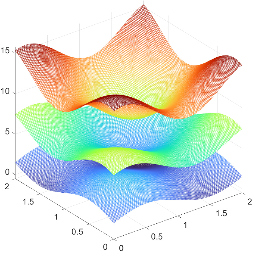
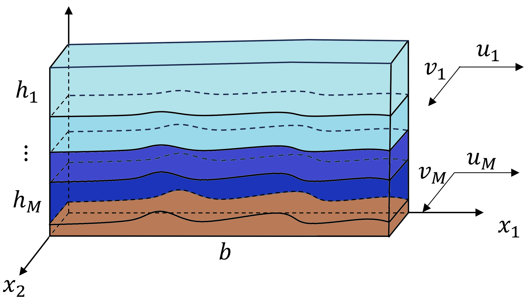
where hm(t,𝒙)0subscript𝑚𝑡𝒙0h_{m}(t,\bm{x})\geqslant 0 is the water depth of the m𝑚mth-layer for m=1,,M𝑚1𝑀m=1,\dots,M, umsubscript𝑢𝑚u_{m} and vmsubscript𝑣𝑚v_{m} are the x1subscript𝑥1x_{1}- and x2subscript𝑥2x_{2}-component of the m𝑚mth-layer fluid velocity, and g𝑔g is the gravitational constant. The density ratio between the k𝑘kth- and m𝑚mth-layer is denoted by rkm=ρk/ρmsubscript𝑟𝑘𝑚subscript𝜌𝑘subscript𝜌𝑚r_{km}=\rho_{k}/\rho_{m}, and the constant densities satisfy 0<ρ1<<ρM0subscript𝜌1subscript𝜌𝑀0<\rho_{1}<\cdots<\rho_{M}. In this paper, the dry water cases are not considered, i.e., hm(t,𝒙)subscript𝑚𝑡𝒙h_{m}(t,\bm{x}) is always positive. An illustration of such a multi-layer system is given in Figure 1.1.
Refer to caption
Figure 1.1: Illustration of the multi-layer shallow water equations.

In real-world applications of oceanography and coastal engineering, numerically solving the ML-SWEs is of great importance. One of the difficulties is that there is no analytical expression for the eigenvalues and eigenvectors of the system (1.1), so that some numerical methods, such as upwind schemes, cannot be directly extended to the multi-layer cases. For the two-layer SWEs (2.8), when |u2u1|subscript𝑢2subscript𝑢1\lvert u_{2}-u_{1}\rvert and 1r121subscript𝑟121-r_{12} are small, an approximation of the eigenvalues is given in [38, 28], and one needs (u1u2)2<g(1r12)(h1+h2)superscriptsubscript𝑢1subscript𝑢22𝑔1subscript𝑟12subscript1subscript2\left(u_{1}-u_{2}\right)^{2}<g(1-r_{12})(h_{1}+h_{2}) to ensure real eigenvalues. But this condition is only valid when r121subscript𝑟121r_{12}\approx 1 and u1u2subscript𝑢1subscript𝑢2u_{1}\approx u_{2}, as stated in [30]. When the number of layers M3𝑀3M\geqslant 3, it is difficult to get an estimation for the eigenvalues [26]. One more practical way is to estimate the upper or lower bounds of the eigenvalues.

Another important issue that should be addressed is that the ML-SWEs (1.1) possess the following lake at rest state

(hm+b+k>mhk+k<mrkmhk)Cm,um=vm=0,m=1,,M,formulae-sequenceformulae-sequencesubscript𝑚𝑏subscript𝑘𝑚subscript𝑘subscript𝑘𝑚subscript𝑟𝑘𝑚subscript𝑘subscript𝐶𝑚subscript𝑢𝑚subscript𝑣𝑚0𝑚1𝑀\left(h_{m}+b+\sum\limits_{k>m}h_{k}+\sum\limits_{k<m}r_{km}h_{k}\right)\equiv C_{m},~{}u_{m}=v_{m}=0,~{}m=1,\cdots,M,

or equivalently,

hm=C~m,m<M,hM+b=C~M,um=vm=0,m=1,,M,formulae-sequenceformulae-sequencesubscript𝑚subscript~𝐶𝑚formulae-sequence𝑚𝑀formulae-sequencesubscript𝑀𝑏subscript~𝐶𝑀subscript𝑢𝑚subscript𝑣𝑚0𝑚1𝑀h_{m}=\widetilde{C}_{m},~{}m<M,~{}h_{M}+b=\widetilde{C}_{M},~{}u_{m}=v_{m}=0,~{}m=1,\cdots,M,

where Cmsubscript𝐶𝑚C_{m} and C~msubscript~𝐶𝑚\widetilde{C}_{m} are constant. Many physical phenomena such as waves on a lake or tsunamis in the deep ocean [11] can be seen as small perturbations of the steady states, and it is crucial to capture these perturbations accurately. This inspired researchers to develop well-balanced (WB) schemes to preserve the steady states in the discrete sense, enabling accurate capture of small perturbations even on coarse meshes. The idea of the WB property or the “C-property” was first illustrated in [3], then various WB numerical methods for the SWEs were studied [43, 47, 2, 33, 37, 45]. For more details, the readers are referred to [29] and the references therein.

Over the past few years, there have been limited numerical schemes introduced for solving the ML-SWEs. The existing schemes have predominantly concentrated on the two-layer scenarios, with minimal attention given to the challenges posed by adaptive moving meshes, not to mention high-order WB and ES adaptive moving mesh schemes for M3𝑀3M\geqslant 3. A relaxation approach [1] was proposed for the 1D two-layer SWEs, which gives an unconditionally hyperbolic system and an explicit eigenstructure. The similar idea was extended to the 2D two-layer case in [16] and [35], where the latter presented a second-order scheme on unstructured meshes. A central-upwind scheme was proposed in [30] based on an estimation of the maximum wave speed and the path-conservative method was employed to improve the robustness of the central-upwind scheme in [14]. A central discontinuous Galerkin (DG) method was constructed for the two-layer SWEs in [15] to achieve high-order accuracy. There are also other works [7, 9, 22, 8, 12].

In the design of numerical methods, it is desirable to satisfy semi-discrete or fully-discrete stability conditions to improve the robustness of the numerical simulations. For hyperbolic conservation laws, the schemes satisfying entropy stability have been extensively studied, e.g., [39, 40, 31, 25, 10, 27, 19]. For the single-layer SWEs, energy stable (ES) schemes that satisfy some discrete energy inequalities were proposed in [4, 24, 7, 51], and recently, high-order WB ES DG schemes were proposed for the two-layer SWEs [23] on fixed curvilinear meshes. The complex structures such as shocks and sharp transitions that arise in solutions to the SWEs often require fine meshes for better resolution. To improve both the efficiency and quality of numerical solutions, the adaptive moving mesh method has been adopted in the numerical simulations for the SWEs. An adaptive moving mesh kinetic flux-vector splitting method was introduced in [41]. High-order adaptive moving mesh DG schemes were proposed in [49, 50], where the preservation of the positivity of the water height and the lake at rest was also discussed. In [48], a WB and positivity-preserving finite volume WENO arbitrary Lagrangian-Eulerian scheme was developed.

This paper aims to develop high-order accurate finite difference schemes for the ML-SWEs that are both ES and WB on fixed and adaptive moving meshes, extending our previous works [20, 51]. To obtain an energy inequality, the convexity of an energy function is proved. Compared to the single-layer case, the coupling terms between the multiple layers in the energy function make the corresponding Hessian matrix more complicated, thus the proof is more involved, which is based on finding the recurrence relations of the leading principal minors or the quadratic forms of the Hessian matrix. The WB property requires compatible discretizations for the flux gradient and source terms, thus a sufficient condition involving the discretizations of the source terms from all the layers is derived for two-point energy conservative (EC) numerical fluxes similar to the single-layer case. The condition can be decomposed into M𝑀M individual equalities for each layer, which makes it convenient to construct M𝑀M two-point fluxes for each single layer, then they are concatenated to form the two-point EC flux for the multi-layer system. Based on such a two-point EC flux, the high-order WB EC fluxes are constructed by using the two-point discretizations as a building block. To suppress possible oscillations near discontinuities, the high-order WB ES schemes are obtained by adding suitable WENO-based dissipation terms to the high-order WB EC fluxes with compatible discretizations of the source terms, which are proved to satisfy semi-discrete energy inequalities. The explicit strong-stability preserving (SSP) third-order Runge-Kutta (RK3) method is employed to obtain the fully-discrete schemes, which are proved to preserve the lake at rest. The extension to the adaptive moving meshes is achieved based on a modified energy function for a reformulated system by including the bottom topography as an additional conservative variable and carefully designed dissipation terms, extending the techniques in [51]. In the numerical experiments for the two- and three-layer systems, the estimation of the maximal wave speed [30] is adopted to choose a proper amount of dissipation since there is no explicit expression for the eigenstructure.

The remainder of this paper is structured as follows. Section 2 presents the proof of the convexity of the energy function and corresponding energy inequality. Section 3 is devoted to the construction of the schemes on fixed meshes. To achieve the WB property, a sufficient condition for the two-point EC fluxes is derived with suitable discretizations of the source terms, and a corresponding two-point EC flux is constructed. Based on such a flux, the high-order WB EC fluxes are obtained, and then the high-order WB ES schemes are developed. The extension of the schemes to adaptive moving meshes is detailed in Section 4 with a modified energy function for the reformulated system. Numerical experiments for the two- and three-layer systems conducted in Section 5 serve to validate the high-order accuracy, efficiency, WB and ES properties, and shock-capturing ability. Section 6 concludes the paper with final remarks.

2 Energy inequality for the ML-SWEs

The ML-SWEs (1.1) can be written in a more compact form

𝑼t+=12𝑭(𝑼)x=g=12m=1Mhm𝑩,m(𝑼,b)x,𝑼𝑡superscriptsubscript12subscript𝑭𝑼subscript𝑥𝑔superscriptsubscript12superscriptsubscript𝑚1𝑀subscript𝑚subscript𝑩𝑚𝑼𝑏subscript𝑥\frac{\partial{\bm{U}}}{\partial t}+\sum_{\ell=1}^{2}\frac{\partial{\bm{F}}_{\ell}({\bm{U}})}{\partial x_{\ell}}=-g\sum_{\ell=1}^{2}\sum\limits_{m=1}^{M}h_{m}\frac{\partial{\bm{B}}_{\ell,m}(\bm{U},b)}{\partial x_{\ell}}, (2.1)

where the vector of the conservative variables 𝑼=(𝑼1T,,𝑼MT)T𝑼superscriptsuperscriptsubscript𝑼1Tsuperscriptsubscript𝑼𝑀TT\bm{U}=(\bm{U}_{1}^{\mathrm{T}},\dots,\bm{U}_{M}^{\mathrm{T}})^{\mathrm{T}} and the xsubscript𝑥x_{\ell}-directional physical flux 𝑭=((𝑭)1T,,(𝑭)MT)Tsubscript𝑭superscriptsuperscriptsubscriptsubscript𝑭1Tsuperscriptsubscriptsubscript𝑭𝑀TT\bm{F}_{\ell}=\left(\left({\bm{F}}_{\ell}\right)_{1}^{\mathrm{T}},\dots,\left({\bm{F}}_{\ell}\right)_{M}^{\mathrm{T}}\right)^{\mathrm{T}} are given by

𝑼m=(hm,hmum,hmvm)T,subscript𝑼𝑚superscriptsubscript𝑚subscript𝑚subscript𝑢𝑚subscript𝑚subscript𝑣𝑚T\displaystyle{\bm{U}_{m}}=\left(h_{m},h_{m}u_{m},h_{m}v_{m}\right)^{\mathrm{T}},
(𝑭1)m=(hmum,hum2+g2hm2,hmumvm)T,subscriptsubscript𝑭1𝑚superscriptsubscript𝑚subscript𝑢𝑚superscriptsubscript𝑢𝑚2𝑔2superscriptsubscript𝑚2subscript𝑚subscript𝑢𝑚subscript𝑣𝑚T\displaystyle\left({\bm{F}}_{1}\right)_{m}=\left(h_{m}u_{m},hu_{m}^{2}+\frac{g}{2}h_{m}^{2},h_{m}u_{m}v_{m}\right)^{\mathrm{T}},
(𝑭2)m=(hmvm,hmumvm,hmvm2+g2hm2)T,subscriptsubscript𝑭2𝑚superscriptsubscript𝑚subscript𝑣𝑚subscript𝑚subscript𝑢𝑚subscript𝑣𝑚subscript𝑚superscriptsubscript𝑣𝑚2𝑔2superscriptsubscript𝑚2T\displaystyle\left({\bm{F}}_{2}\right)_{m}=\left(h_{m}v_{m},h_{m}u_{m}v_{m},h_{m}v_{m}^{2}+\frac{g}{2}h_{m}^{2}\right)^{\mathrm{T}},

with the source terms

𝑩1,msubscript𝑩1𝑚\displaystyle\bm{{B}}_{1,m} =(𝟎3m2,zm,0,𝟎3M3m)T,absentsuperscriptsubscript03𝑚2subscript𝑧𝑚0subscript03𝑀3𝑚T\displaystyle=\left(\bm{0}_{3m-2},z_{m},0,\bm{0}_{3M-3m}\right)^{\mathrm{T}},
𝑩2,msubscript𝑩2𝑚\displaystyle\bm{{B}}_{2,m} =(𝟎3m2,0,zm,𝟎3M3m)T.absentsuperscriptsubscript03𝑚20subscript𝑧𝑚subscript03𝑀3𝑚T\displaystyle=\left(\bm{0}_{3m-2},0,z_{m},\bm{0}_{3M-3m}\right)^{\mathrm{T}}.

Here zm:=b+k>mhk+k<mrkmhkassignsubscript𝑧𝑚𝑏subscript𝑘𝑚subscript𝑘subscript𝑘𝑚subscript𝑟𝑘𝑚subscript𝑘z_{m}:=b+\sum\limits_{k>m}h_{k}+\sum\limits_{k<m}r_{km}h_{k} and 𝟎dsubscript0𝑑\bm{0}_{d} is the row vector with d𝑑d zeros. One can define an energy and energy flux pair for the system (2.1) as

η(𝑼)𝜂𝑼\displaystyle{\eta}({\bm{U}}) :=m=1Mρm2(hmum2+hmvm2+ghm2)+gm=1Mρmhmb+gm=1Mk<mρkhkhm,assignabsentsuperscriptsubscript𝑚1𝑀subscript𝜌𝑚2subscript𝑚superscriptsubscript𝑢𝑚2subscript𝑚superscriptsubscript𝑣𝑚2𝑔superscriptsubscript𝑚2𝑔superscriptsubscript𝑚1𝑀subscript𝜌𝑚subscript𝑚𝑏𝑔superscriptsubscript𝑚1𝑀subscript𝑘𝑚subscript𝜌𝑘subscript𝑘subscript𝑚\displaystyle:=\sum\limits_{m=1}^{M}\dfrac{\rho_{m}}{2}\left(h_{m}u_{m}^{2}+h_{m}v_{m}^{2}+gh_{m}^{2}\right)+g\sum\limits_{m=1}^{M}\rho_{m}h_{m}b+g\sum\limits_{m=1}^{M}\sum\limits_{k<m}\rho_{k}h_{k}h_{m}, (2.2)
q1(𝑼)subscript𝑞1𝑼\displaystyle{q}_{1}({\bm{U}}) :=m=1Mρm2um(hmum2+hmvm2)+gm=1Mρmhm2um+gm=1Mρmhmumzm,assignabsentsuperscriptsubscript𝑚1𝑀subscript𝜌𝑚2subscript𝑢𝑚subscript𝑚superscriptsubscript𝑢𝑚2subscript𝑚superscriptsubscript𝑣𝑚2𝑔superscriptsubscript𝑚1𝑀subscript𝜌𝑚superscriptsubscript𝑚2subscript𝑢𝑚𝑔superscriptsubscript𝑚1𝑀subscript𝜌𝑚subscript𝑚subscript𝑢𝑚subscript𝑧𝑚\displaystyle:=\sum\limits_{m=1}^{M}\dfrac{\rho_{m}}{2}u_{m}\left(h_{m}u_{m}^{2}+h_{m}v_{m}^{2}\right)+g\sum\limits_{m=1}^{M}\rho_{m}h_{m}^{2}u_{m}+g\sum\limits_{m=1}^{M}\rho_{m}h_{m}u_{m}z_{m},
q2(𝑼)subscript𝑞2𝑼\displaystyle{q}_{2}({\bm{U}}) :=m=1Mρm2vm(hmum2+hmvm2)+gm=1Mρmhm2vm+gm=1Mρmhmvmzm,assignabsentsuperscriptsubscript𝑚1𝑀subscript𝜌𝑚2subscript𝑣𝑚subscript𝑚superscriptsubscript𝑢𝑚2subscript𝑚superscriptsubscript𝑣𝑚2𝑔superscriptsubscript𝑚1𝑀subscript𝜌𝑚superscriptsubscript𝑚2subscript𝑣𝑚𝑔superscriptsubscript𝑚1𝑀subscript𝜌𝑚subscript𝑚subscript𝑣𝑚subscript𝑧𝑚\displaystyle:=\sum\limits_{m=1}^{M}\dfrac{\rho_{m}}{2}v_{m}\left(h_{m}u_{m}^{2}+h_{m}v_{m}^{2}\right)+g\sum\limits_{m=1}^{M}\rho_{m}h_{m}^{2}v_{m}+g\sum\limits_{m=1}^{M}\rho_{m}h_{m}v_{m}z_{m},

which satisfies the following consistent condition

q𝑼=η𝑼(𝑭𝑼+𝑵),=1,2,formulae-sequencesubscript𝑞𝑼𝜂𝑼subscript𝑭𝑼subscript𝑵12\dfrac{\partial{{q}_{\ell}}}{\partial{{\bm{U}}}}=\dfrac{\partial{\eta}}{\partial{\bm{U}}}\left(\dfrac{\partial{{\bm{F}}_{\ell}}}{\partial{{\bm{U}}}}+\bm{N}_{\ell}\right),~{}\ell=1,2, (2.3)

where 𝑵(𝑼,b)subscript𝑵𝑼𝑏\bm{N}_{\ell}\left(\bm{U},b\right) comes from the non-conservative source terms

𝑵=gm=1Mhm𝑩,m𝑼.subscript𝑵𝑔superscriptsubscript𝑚1𝑀subscript𝑚subscript𝑩𝑚𝑼\bm{N}_{\ell}=g\sum_{m=1}^{M}h_{m}\dfrac{\partial{\bm{B}_{{\ell},m}}}{\partial{\bm{U}}}.

The convexity of the energy η𝜂\eta with respect to 𝑼𝑼\bm{U} is proved in Proposition 2.1, based on the structure of the Hessian matrix 2η/𝑼2superscript2𝜂superscript𝑼2\partial^{2}{\eta}/\partial{\bm{U}}^{2} given in Lemma 2.1.

Lemma 2.1.

Denote the Hessian matrix for the 𝒩𝒩\mathcal{N}-layer case as 𝒩3𝒩×3𝒩subscript𝒩superscript3𝒩3𝒩\mathcal{M}_{\mathcal{N}}\in\mathbb{R}^{3\mathcal{N}\times 3\mathcal{N}}, then the Hessian matrix for the (𝒩+1)𝒩1(\mathcal{N}+1)-layer case can be expressed as

𝒩+1=(𝒩A1TA1A2)(3𝒩+3)×(3𝒩+3),subscript𝒩1subscript𝒩superscriptsubscript𝐴1Tsubscript𝐴1subscript𝐴2superscript3𝒩33𝒩3\mathcal{M}_{\mathcal{N}+1}=\left(\begin{array}[]{cc}\mathcal{M}_{\mathcal{N}}&A_{1}^{\mathrm{T}}\\ A_{1}&A_{2}\end{array}\right)\in\mathbb{R}^{(3\mathcal{N}+3)\times(3\mathcal{N}+3)},

where

A1=(gρ100gρ200gρ𝒩100gρ𝒩00000000000000000000000000)3×3𝒩,subscript𝐴1𝑔subscript𝜌100𝑔subscript𝜌200𝑔subscript𝜌𝒩100𝑔subscript𝜌𝒩00missing-subexpression000000000000missing-subexpression000000000000missing-subexpressionsuperscript33𝒩\displaystyle A_{1}=\left(\begin{array}[]{cccccccccccccc}g\rho_{1}&0&0&g\rho_{2}&0&0&\cdots&g\rho_{\mathcal{N}-1}&0&0&g\rho_{\mathcal{N}}&0&0\\ 0&0&0&0&0&0&\cdots&0&0&0&0&0&0\\ 0&0&0&0&0&0&\cdots&0&0&0&0&0&0\end{array}\right)\in\mathbb{R}^{3\times 3\mathcal{N}},
A2=(ρ𝒩+1(u𝒩+12+v𝒩+12+gh𝒩+1)h𝒩+1ρ𝒩+1u𝒩+1h𝒩+1ρ𝒩+1v𝒩+1h𝒩+1ρ𝒩+1u𝒩+1h𝒩+1ρ𝒩+1h𝒩+10ρ𝒩+1v𝒩+1h𝒩+10ρ𝒩+1h𝒩+1)3×3.subscript𝐴2subscript𝜌𝒩1superscriptsubscript𝑢𝒩12superscriptsubscript𝑣𝒩12𝑔subscript𝒩1subscript𝒩1subscript𝜌𝒩1subscript𝑢𝒩1subscript𝒩1subscript𝜌𝒩1subscript𝑣𝒩1subscript𝒩1subscript𝜌𝒩1subscript𝑢𝒩1subscript𝒩1subscript𝜌𝒩1subscript𝒩10subscript𝜌𝒩1subscript𝑣𝒩1subscript𝒩10subscript𝜌𝒩1subscript𝒩1superscript33\displaystyle A_{2}=\left(\begin{array}[]{ccc}\frac{\rho_{\mathcal{N}+1}\,\left(u_{\mathcal{N}+1}^{2}+v_{\mathcal{N}+1}^{2}+g\,h_{\mathcal{N}+1}\right)}{h_{\mathcal{N}+1}}&-\frac{\rho_{\mathcal{N}+1}\,u_{\mathcal{N}+1}}{h_{\mathcal{N}+1}}&-\frac{\rho_{\mathcal{N}+1}\,v_{\mathcal{N}+1}}{h_{\mathcal{N}+1}}\\ -\frac{\rho_{\mathcal{N}+1}\,u_{\mathcal{N}+1}}{h_{\mathcal{N}+1}}&\frac{\rho_{\mathcal{N}+1}}{h_{\mathcal{N}+1}}&0\\ -\frac{\rho_{\mathcal{N}+1}\,v_{\mathcal{N}+1}}{h_{\mathcal{N}+1}}&0&\frac{\rho_{\mathcal{N}+1}}{h_{\mathcal{N}+1}}\end{array}\right)\in\mathbb{R}^{3\times 3}.
Proof.

It can be completed because the Hessian matrices 𝒩subscript𝒩\mathcal{M}_{\mathcal{N}} and 𝒩+1subscript𝒩1\mathcal{M}_{\mathcal{N}+1} can be calculated directly. ∎

Proposition 2.1.

Under the condition 0<ρ1<ρ2<<ρ𝒩<0subscript𝜌1subscript𝜌2subscript𝜌𝒩0<\rho_{1}<\rho_{2}<\dots<\rho_{\mathcal{N}}<\dots, the energy η𝜂\eta is convex with respect to 𝑼𝑼\bm{U}, i.e., the Hessian matrix 𝒩=2η/𝑼2subscript𝒩superscript2𝜂superscript𝑼2\mathcal{M}_{\mathcal{N}}=\partial^{2}{\eta}/\partial{\bm{U}}^{2} is positive-definite. Moreover, the determinant of 𝒩subscript𝒩\mathcal{M}_{\mathcal{N}} is

det(𝒩)=g𝒩ρ13m=2𝒩ρm2(ρmρm1)m=1𝒩hm2.subscript𝒩superscript𝑔𝒩superscriptsubscript𝜌13superscriptsubscriptproduct𝑚2𝒩superscriptsubscript𝜌𝑚2subscript𝜌𝑚subscript𝜌𝑚1superscriptsubscriptproduct𝑚1𝒩superscriptsubscript𝑚2\det(\mathcal{M}_{\mathcal{N}})=\frac{g^{\mathcal{N}}\rho_{1}^{3}\prod_{m=2}^{\mathcal{N}}\rho_{m}^{2}(\rho_{m}-\rho_{m-1})}{\prod_{m=1}^{\mathcal{N}}h_{m}^{2}}. (2.4)
Proof.

The proof is given by induction on 𝒩𝒩\mathcal{N}. When 𝒩=2𝒩2\mathcal{N}=2, one observes that the Hessian matrix 2subscript2\mathcal{M}_{2} is

2=(ρ1(u12+v12+gh1)h1ρ1u1h1ρ1v1h1gρ100ρ1u1h1ρ1h10000ρ1v1h10ρ1h1000gρ100ρ2(u22+v22+gh2)h2ρ2u2h2ρ2v2h2000ρ2u2h2ρ2h20000ρ2v2h20ρ2h2).subscript2subscript𝜌1superscriptsubscript𝑢12superscriptsubscript𝑣12𝑔subscript1subscript1subscript𝜌1subscript𝑢1subscript1subscript𝜌1subscript𝑣1subscript1𝑔subscript𝜌100subscript𝜌1subscript𝑢1subscript1subscript𝜌1subscript10000subscript𝜌1subscript𝑣1subscript10subscript𝜌1subscript1000𝑔subscript𝜌100subscript𝜌2superscriptsubscript𝑢22superscriptsubscript𝑣22𝑔subscript2subscript2subscript𝜌2subscript𝑢2subscript2subscript𝜌2subscript𝑣2subscript2000subscript𝜌2subscript𝑢2subscript2subscript𝜌2subscript20000subscript𝜌2subscript𝑣2subscript20subscript𝜌2subscript2\mathcal{M}_{2}=\left(\begin{array}[]{cccccc}\frac{\rho_{1}\,\left(u_{1}^{2}+v_{1}^{2}+g\,h_{1}\right)}{h_{1}}&-\frac{\rho_{1}\,u_{1}}{h_{1}}&-\frac{\rho_{1}\,v_{1}}{h_{1}}&g\,\rho_{1}&0&0\\ -\frac{\rho_{1}\,u_{1}}{h_{1}}&\frac{\rho_{1}}{h_{1}}&0&0&0&0\\ -\frac{\rho_{1}\,v_{1}}{h_{1}}&0&\frac{\rho_{1}}{h_{1}}&0&0&0\\ g\,\rho_{1}&0&0&\frac{\rho_{2}\,\left(u_{2}^{2}+v_{2}^{2}+g\,h_{2}\right)}{h_{2}}&-\frac{\rho_{2}\,u_{2}}{h_{2}}&-\frac{\rho_{2}\,v_{2}}{h_{2}}\\ 0&0&0&-\frac{\rho_{2}\,u_{2}}{h_{2}}&\frac{\rho_{2}}{h_{2}}&0\\ 0&0&0&-\frac{\rho_{2}\,v_{2}}{h_{2}}&0&\frac{\rho_{2}}{h_{2}}\end{array}\right). (2.5)

Denote the leading principal minors of order m𝑚m as 𝒟msubscript𝒟𝑚\mathcal{D}_{m}, then the leading principal minors of 2subscript2\mathcal{M}_{2} are

𝒟1=ρ1(u12+v12+gh1)h1,𝒟2=ρ12v12+gh1ρ12h12,𝒟3=gρ13h12,formulae-sequencesubscript𝒟1subscript𝜌1superscriptsubscript𝑢12superscriptsubscript𝑣12𝑔subscript1subscript1formulae-sequencesubscript𝒟2superscriptsubscript𝜌12superscriptsubscript𝑣12𝑔subscript1superscriptsubscript𝜌12superscriptsubscript12subscript𝒟3𝑔superscriptsubscript𝜌13superscriptsubscript12\displaystyle\mathcal{D}_{1}=\frac{\rho_{1}\left(u_{1}^{2}+v_{1}^{2}+gh_{1}\right)}{h_{1}},~{}\mathcal{D}_{2}=\frac{\rho_{1}^{2}v_{1}^{2}+gh_{1}\rho_{1}^{2}}{h_{1}^{2}},~{}\mathcal{D}_{3}=\frac{g\rho_{1}^{3}}{h_{1}^{2}},
𝒟4=gρ13(gh2(ρ2ρ1)+ρ2(u22+v22))h12h2,𝒟5=gρ13ρ2(gh2(ρ2ρ1)+ρ2v22)h12h22,formulae-sequencesubscript𝒟4𝑔superscriptsubscript𝜌13𝑔subscript2subscript𝜌2subscript𝜌1subscript𝜌2superscriptsubscript𝑢22superscriptsubscript𝑣22superscriptsubscript12subscript2subscript𝒟5𝑔superscriptsubscript𝜌13subscript𝜌2𝑔subscript2subscript𝜌2subscript𝜌1subscript𝜌2superscriptsubscript𝑣22superscriptsubscript12superscriptsubscript22\displaystyle\mathcal{D}_{4}=\frac{g\rho_{1}^{3}\left(gh_{2}\left(\rho_{2}-\rho_{1}\right)+\rho_{2}\left(u_{2}^{2}+v_{2}^{2}\right)\right)}{h_{1}^{2}\,h_{2}},~{}\mathcal{D}_{5}=\frac{g\rho_{1}^{3}\rho_{2}\left(gh_{2}\left(\rho_{2}-\rho_{1}\right)+\rho_{2}v_{2}^{2}\right)}{h_{1}^{2}h_{2}^{2}},
𝒟6=g2ρ13ρ22(ρ2ρ1)h12h22,subscript𝒟6superscript𝑔2superscriptsubscript𝜌13superscriptsubscript𝜌22subscript𝜌2subscript𝜌1superscriptsubscript12superscriptsubscript22\displaystyle\mathcal{D}_{6}=\frac{g^{2}\rho_{1}^{3}\,\rho_{2}^{2}\,\left(\rho_{2}-\rho_{1}\right)}{h_{1}^{2}\,h_{2}^{2}},

which are all positive as 0<ρ1<ρ20subscript𝜌1subscript𝜌20<\rho_{1}<\rho_{2}, thus the matrix 2subscript2\mathcal{M}_{2} is positive-definite.

Now it suffices to show that if 𝒩subscript𝒩\mathcal{M}_{\mathcal{N}} is positive-definite and its determinant is (2.4), then the conclusion also holds for the (𝒩+1)𝒩1(\mathcal{N}+1)-layer case. The first 3𝒩3𝒩3\mathcal{N} leading principal minors of 𝒩+1subscript𝒩1\mathcal{M}_{\mathcal{N}+1} are also those of 𝒩subscript𝒩\mathcal{M}_{\mathcal{N}}, thus they are positive. According to the matrix structure in Lemma 2.1, one can calculate 𝒟3𝒩+1subscript𝒟3𝒩1\mathcal{D}_{3\mathcal{N}+1} by expanding along the (3𝒩+1)3𝒩1(3\mathcal{N}+1)th column to obtain

𝒟3𝒩+1=subscript𝒟3𝒩1absent\displaystyle\mathcal{D}_{3\mathcal{N}+1}= ρ𝒩+1(u𝒩+12+v𝒩+12+gh𝒩+1)h𝒩+1det(𝒩)subscript𝜌𝒩1superscriptsubscript𝑢𝒩12superscriptsubscript𝑣𝒩12𝑔subscript𝒩1subscript𝒩1subscript𝒩\displaystyle\ \frac{\rho_{\mathcal{N}+1}\,\left(u_{\mathcal{N}+1}^{2}+v_{\mathcal{N}+1}^{2}+g\,h_{\mathcal{N}+1}\right)}{h_{\mathcal{N}+1}}\det(\mathcal{M}_{\mathcal{N}})
+m=1𝒩(1)3𝒩+3m1gρmdet(𝒩~[3m2;3𝒩+1]),superscriptsubscript𝑚1𝒩superscript13𝒩3𝑚1𝑔subscript𝜌𝑚~𝒩3𝑚23𝒩1\displaystyle+\sum_{m=1}^{\mathcal{N}}(-1)^{3\mathcal{N}+3m-1}g\rho_{m}\det\left(\widetilde{\mathcal{\mathcal{N}}}[3m-2;3\mathcal{N}+1]\right),

where ~[3m2;3𝒩+1]3𝒩×3𝒩~3𝑚23𝒩1superscript3𝒩3𝒩\widetilde{\mathcal{M}}[3m-2;3\mathcal{N}+1]\in\mathbb{R}^{3\mathcal{N}\times 3\mathcal{N}} represents the submatrix obtained by removing the (3m2)3𝑚2(3m-2)th row and (3𝒩+1)3𝒩1(3\mathcal{N}+1)th column in the upper left (3𝒩+1)×(3𝒩+1)3𝒩13𝒩1(3\mathcal{N}+1)\times(3\mathcal{N}+1) submatrix of 𝒩+1subscript𝒩1\mathcal{M}_{\mathcal{N}+1}. When m<𝒩𝑚𝒩m<\mathcal{N}, the last four rows in ~[3m2;3𝒩+1]~3𝑚23𝒩1\widetilde{\mathcal{M}}[3m-2;3\mathcal{N}+1] are

1=(gρ1,0,0,gρ2,0,0,,gρ𝒩1,0,0,ρ𝒩(u𝒩2+v𝒩2+gh𝒩)h𝒩,ρ𝒩u𝒩h𝒩,ρ𝒩v𝒩h𝒩),subscript1𝑔subscript𝜌100𝑔subscript𝜌200𝑔subscript𝜌𝒩100subscript𝜌𝒩superscriptsubscript𝑢𝒩2superscriptsubscript𝑣𝒩2𝑔subscript𝒩subscript𝒩subscript𝜌𝒩subscript𝑢𝒩subscript𝒩subscript𝜌𝒩subscript𝑣𝒩subscript𝒩\displaystyle\mathcal{I}_{1}=\left(g\rho_{1},~{}0,~{}0,~{}g\rho_{2},~{}0,~{}0,~{}\cdots,~{}g\rho_{\mathcal{N}-1},~{}0,~{}0,~{}\frac{\rho_{\mathcal{N}}(u_{\mathcal{N}}^{2}+v_{\mathcal{N}}^{2}+gh_{\mathcal{N}})}{h_{\mathcal{N}}},~{}-\frac{\rho_{\mathcal{N}}u_{\mathcal{N}}}{h_{\mathcal{N}}},~{}-\frac{\rho_{\mathcal{N}}v_{\mathcal{N}}}{h_{\mathcal{N}}}\right),~{}
2=(0,0,0,0,0,0,,0,0,0,ρ𝒩u𝒩h𝒩,ρ𝒩h𝒩,0),subscript2000000000subscript𝜌𝒩subscript𝑢𝒩subscript𝒩subscript𝜌𝒩subscript𝒩0\displaystyle\mathcal{I}_{2}=\left(0,~{}0,~{}0,~{}0,~{}0,~{}0,~{}\cdots,~{}0,~{}0,~{}0,~{}-\frac{\rho_{\mathcal{N}}u_{\mathcal{N}}}{h_{\mathcal{N}}},~{}\frac{\rho_{\mathcal{N}}}{h_{\mathcal{N}}},~{}0\right),
3=(0,0,0,0,0,0,,0,0,0,ρ𝒩v𝒩h𝒩,0,ρ𝒩h𝒩),subscript3000000000subscript𝜌𝒩subscript𝑣𝒩subscript𝒩0subscript𝜌𝒩subscript𝒩\displaystyle\mathcal{I}_{3}=\left(0,~{}0,~{}0,~{}0,~{}0,~{}0,~{}\cdots,~{}0,~{}0,~{}0,~{}-\frac{\rho_{\mathcal{N}}v_{\mathcal{N}}}{h_{\mathcal{N}}},~{}0,~{}\frac{\rho_{\mathcal{N}}}{h_{\mathcal{N}}}\right),~{}
4=(gρ1,0,0,gρ2,0,0,,gρ𝒩1,0,0,gρ𝒩,0,0),subscript4𝑔subscript𝜌100𝑔subscript𝜌200𝑔subscript𝜌𝒩100𝑔subscript𝜌𝒩00\displaystyle\mathcal{I}_{4}=\left(g\rho_{1},~{}0,~{}0,~{}g\rho_{2},~{}0,~{}0,~{}\cdots,~{}g\rho_{\mathcal{N}-1},~{}0,~{}0,~{}g\rho_{\mathcal{N}},~{}0,~{}0\right),

which are linear dependent as 1=4u𝒩2v𝒩3subscript1subscript4subscript𝑢𝒩subscript2subscript𝑣𝒩subscript3\mathcal{I}_{1}=\mathcal{I}_{4}-u_{\mathcal{N}}\mathcal{I}_{2}-v_{\mathcal{N}}\mathcal{I}_{3}, thus det(~[3m2;3𝒩+1])=0~3𝑚23𝒩10\det\left(\widetilde{\mathcal{M}}[3m-2;3\mathcal{N}+1]\right)=0 for m<𝒩𝑚𝒩m<\mathcal{N}. When m=𝒩𝑚𝒩m=\mathcal{N}, the last three rows in ~[3m2;3𝒩+1]~3𝑚23𝒩1\widetilde{\mathcal{M}}[3m-2;3\mathcal{N}+1] are

(0,0,0,0,0,0,,0,0,0,ρ𝒩u𝒩h𝒩,ρ𝒩h𝒩,0),000000000subscript𝜌𝒩subscript𝑢𝒩subscript𝒩subscript𝜌𝒩subscript𝒩0\displaystyle\left(0,~{}0,~{}0,~{}0,~{}0,~{}0,~{}\cdots,~{}0,~{}0,~{}0,~{}-\frac{\rho_{\mathcal{N}}u_{\mathcal{N}}}{h_{\mathcal{N}}},~{}\frac{\rho_{\mathcal{N}}}{h_{\mathcal{N}}},~{}0\right),~{}
(0,0,0,0,0,0,,0,0,0,ρ𝒩v𝒩h𝒩,0,ρ𝒩h𝒩),000000000subscript𝜌𝒩subscript𝑣𝒩subscript𝒩0subscript𝜌𝒩subscript𝒩\displaystyle\left(0,~{}0,~{}0,~{}0,~{}0,~{}0,~{}\cdots,~{}0,~{}0,~{}0,~{}-\frac{\rho_{\mathcal{N}}v_{\mathcal{N}}}{h_{\mathcal{N}}},~{}0,~{}\frac{\rho_{\mathcal{N}}}{h_{\mathcal{N}}}~{}\right),~{}
(gρ1,0,0,gρ2,0,0,,gρ𝒩1,0,0,gρ𝒩,0,0).𝑔subscript𝜌100𝑔subscript𝜌200𝑔subscript𝜌𝒩100𝑔subscript𝜌𝒩00\displaystyle\left(g\rho_{1},~{}0,~{}0,~{}g\rho_{2},~{}0,~{}0,~{}\cdots,~{}g\rho_{\mathcal{N}-1},~{}0,~{}0,~{}g\rho_{\mathcal{N}},~{}0,~{}0\right).

After some matrix operations, they become

(gρ1,0,0,gρ2,0,0,,gρ𝒩1,0,0,ρ𝒩(u𝒩2+v𝒩2+gh𝒩)h𝒩,ρ𝒩u𝒩h𝒩,ρ𝒩v𝒩h𝒩),𝑔subscript𝜌100𝑔subscript𝜌200𝑔subscript𝜌𝒩100subscript𝜌𝒩superscriptsubscript𝑢𝒩2superscriptsubscript𝑣𝒩2𝑔subscript𝒩subscript𝒩subscript𝜌𝒩subscript𝑢𝒩subscript𝒩subscript𝜌𝒩subscript𝑣𝒩subscript𝒩\displaystyle\left(g\rho_{1},~{}0,~{}0,~{}g\rho_{2},~{}0,~{}0,~{}\cdots,~{}g\rho_{\mathcal{N}-1},~{}0,~{}0,~{}\frac{\rho_{\mathcal{N}}(u_{\mathcal{N}}^{2}+v_{\mathcal{N}}^{2}+gh_{\mathcal{N}})}{h_{\mathcal{N}}},~{}-\frac{\rho_{\mathcal{N}}u_{\mathcal{N}}}{h_{\mathcal{N}}},~{}-\frac{\rho_{\mathcal{N}}v_{\mathcal{N}}}{h_{\mathcal{N}}}\right),~{}
(0,0,0,0,0,0,,0,0,0,ρ𝒩u𝒩h𝒩,ρ𝒩h𝒩,0),000000000subscript𝜌𝒩subscript𝑢𝒩subscript𝒩subscript𝜌𝒩subscript𝒩0\displaystyle\left(0,~{}0,~{}0,~{}0,~{}0,~{}0,~{}\cdots,~{}0,~{}0,~{}0,~{}-\frac{\rho_{\mathcal{N}}u_{\mathcal{N}}}{h_{\mathcal{N}}},~{}\frac{\rho_{\mathcal{N}}}{h_{\mathcal{N}}},~{}0\right),
(0,0,0,0,0,0,,0,0,0,ρ𝒩v𝒩h𝒩,0,ρ𝒩h𝒩),000000000subscript𝜌𝒩subscript𝑣𝒩subscript𝒩0subscript𝜌𝒩subscript𝒩\displaystyle\left(0,~{}0,~{}0,~{}0,~{}0,~{}0,~{}\cdots,~{}0,~{}0,~{}0,~{}-\frac{\rho_{\mathcal{N}}v_{\mathcal{N}}}{h_{\mathcal{N}}},~{}0,~{}\frac{\rho_{\mathcal{N}}}{h_{\mathcal{N}}}\right),

which recover the last three rows in 𝒩subscript𝒩\mathcal{M}_{\mathcal{N}}, and the determinant of ~[3m2;3𝒩+1]~3𝑚23𝒩1\widetilde{\mathcal{M}}[3m-2;3\mathcal{N}+1] remains the same, so that

gρ𝒩det(~[3m2;3𝒩+1])=gρ𝒩det(𝒩),𝑔subscript𝜌𝒩~3𝑚23𝒩1𝑔subscript𝜌𝒩subscript𝒩g\rho_{\mathcal{N}}\det\left(\widetilde{\mathcal{M}}[3m-2;3\mathcal{N}+1]\right)=g\rho_{\mathcal{N}}\det\left(\mathcal{M}_{\mathcal{N}}\right),

and

𝒟3𝒩+1=ρ𝒩+1(u𝒩+12+v𝒩+12+gh𝒩+1)h𝒩+1det(𝒩)gρ𝒩det(𝒩).subscript𝒟3𝒩1subscript𝜌𝒩1superscriptsubscript𝑢𝒩12superscriptsubscript𝑣𝒩12𝑔subscript𝒩1subscript𝒩1subscript𝒩𝑔subscript𝜌𝒩subscript𝒩\displaystyle\mathcal{D}_{3\mathcal{N}+1}=\frac{\rho_{\mathcal{N}+1}\,\left(u_{\mathcal{N}+1}^{2}+v_{\mathcal{N}+1}^{2}+gh_{\mathcal{N}+1}\right)}{h_{\mathcal{N}+1}}\det(\mathcal{M}_{\mathcal{N}})-g\rho_{\mathcal{N}}\det(\mathcal{M}_{\mathcal{N}}).

It is straightforward to obtain the expressions of the last two leading principal minors,

𝒟3𝒩+2=ρ𝒩+1h𝒩+1𝒟3𝒩+1ρ𝒩+12u𝒩+12h𝒩+12det(𝒩),subscript𝒟3𝒩2subscript𝜌𝒩1subscript𝒩1subscript𝒟3𝒩1superscriptsubscript𝜌𝒩12superscriptsubscript𝑢𝒩12superscriptsubscript𝒩12subscript𝒩\displaystyle\mathcal{D}_{3\mathcal{N}+2}=\frac{\rho_{\mathcal{N}+1}}{h_{\mathcal{N}+1}}\mathcal{D}_{3\mathcal{N}+1}-\frac{\rho_{\mathcal{N}+1}^{2}u_{\mathcal{N}+1}^{2}}{h_{\mathcal{N}+1}^{2}}\det(\mathcal{M}_{\mathcal{N}}),
𝒟3𝒩+3=ρ𝒩+1h𝒩+1𝒟3𝒩+2ρ𝒩+13v𝒩+12h𝒩+13det(𝒩).subscript𝒟3𝒩3subscript𝜌𝒩1subscript𝒩1subscript𝒟3𝒩2superscriptsubscript𝜌𝒩13superscriptsubscript𝑣𝒩12superscriptsubscript𝒩13subscript𝒩\displaystyle\mathcal{D}_{3\mathcal{N}+3}=\frac{\rho_{\mathcal{N}+1}}{h_{\mathcal{N}+1}}\mathcal{D}_{3\mathcal{N}+2}-\frac{\rho_{\mathcal{N}+1}^{3}v_{\mathcal{N}+1}^{2}}{h_{\mathcal{N}+1}^{3}}\det(\mathcal{M}_{\mathcal{N}}).

Using (2.4) yields

𝒟3𝒩+1=subscript𝒟3𝒩1absent\displaystyle\mathcal{D}_{3\mathcal{N}+1}= (ρ𝒩+1(u𝒩+12+v𝒩+12)+gh𝒩+1(ρ𝒩+1ρ𝒩))g𝒩ρ13m=2𝒩ρm2(ρmρm1)h𝒩+1m=1𝒩hm2,subscript𝜌𝒩1superscriptsubscript𝑢𝒩12superscriptsubscript𝑣𝒩12𝑔subscript𝒩1subscript𝜌𝒩1subscript𝜌𝒩superscript𝑔𝒩superscriptsubscript𝜌13superscriptsubscriptproduct𝑚2𝒩superscriptsubscript𝜌𝑚2subscript𝜌𝑚subscript𝜌𝑚1subscript𝒩1superscriptsubscriptproduct𝑚1𝒩superscriptsubscript𝑚2\displaystyle\frac{\left(\rho_{\mathcal{N}+1}(u_{\mathcal{N}+1}^{2}+v_{\mathcal{N}+1}^{2})+gh_{\mathcal{N}+1}(\rho_{\mathcal{N}+1}-\rho_{\mathcal{N}})\right)g^{\mathcal{N}}\rho_{1}^{3}\prod_{m=2}^{\mathcal{N}}\rho_{m}^{2}(\rho_{m}-\rho_{m-1})}{h_{\mathcal{N}+1}\prod_{m=1}^{\mathcal{N}}h_{m}^{2}},
𝒟3𝒩+2=subscript𝒟3𝒩2absent\displaystyle\mathcal{D}_{3\mathcal{N}+2}= ρ𝒩+1(ρ𝒩+1v𝒩+12+gh𝒩+1(ρ𝒩+1ρ𝒩))g𝒩ρ13m=2𝒩ρm2(ρmρm1)m=1𝒩+1hm2,subscript𝜌𝒩1subscript𝜌𝒩1superscriptsubscript𝑣𝒩12𝑔subscript𝒩1subscript𝜌𝒩1subscript𝜌𝒩superscript𝑔𝒩superscriptsubscript𝜌13superscriptsubscriptproduct𝑚2𝒩superscriptsubscript𝜌𝑚2subscript𝜌𝑚subscript𝜌𝑚1superscriptsubscriptproduct𝑚1𝒩1superscriptsubscript𝑚2\displaystyle\frac{\rho_{\mathcal{N}+1}(\rho_{\mathcal{N}+1}v_{\mathcal{N}+1}^{2}+gh_{\mathcal{N}+1}(\rho_{\mathcal{N}+1}-\rho_{\mathcal{N}}))g^{\mathcal{N}}\rho_{1}^{3}\prod_{m=2}^{\mathcal{N}}\rho_{m}^{2}(\rho_{m}-\rho_{m-1})}{\prod_{m=1}^{\mathcal{N}+1}h_{m}^{2}},
𝒟3𝒩+3=subscript𝒟3𝒩3absent\displaystyle\mathcal{D}_{3\mathcal{N}+3}= g𝒩+1ρ13m=2𝒩+1ρm2(ρmρm1)m=1𝒩+1hm2,superscript𝑔𝒩1superscriptsubscript𝜌13superscriptsubscriptproduct𝑚2𝒩1superscriptsubscript𝜌𝑚2subscript𝜌𝑚subscript𝜌𝑚1superscriptsubscriptproduct𝑚1𝒩1superscriptsubscript𝑚2\displaystyle\frac{g^{\mathcal{N}+1}\rho_{1}^{3}\prod_{m=2}^{\mathcal{N}+1}\rho_{m}^{2}(\rho_{m}-\rho_{m-1})}{\prod_{m=1}^{\mathcal{N}+1}h_{m}^{2}},

which are all positive, and (2.4) also holds for the (𝒩+1)𝒩1(\mathcal{N}+1)-layer case when 𝒩𝒩\mathcal{N} is replaced by 𝒩+1𝒩1\mathcal{N}+1. ∎

Remark 2.1.

One can also prove the convexity of the energy function by finding the recurrence relations of the quadratic forms of the Hessian matrix, with more details in A.

Based on the convexity of η𝜂\eta and the consistent condition (2.3), the following energy inequality is satisfied

η(𝑼)t+=12q(𝑼)x0,𝜂𝑼𝑡superscriptsubscript12subscript𝑞𝑼subscript𝑥0\frac{\partial{\eta}({\bm{U}})}{\partial t}+\sum_{\ell=1}^{2}\frac{\partial{q}_{\ell}({\bm{U}})}{\partial x_{\ell}}\leqslant 0,

where the equality holds only when the solutions are smooth and the inequality holds in the distribution sense. For clarity of notations, define 𝑽:=(𝑽1,,𝑽M)T=(η/𝑼)Tassign𝑽superscriptsubscript𝑽1subscript𝑽𝑀Tsuperscript𝜂𝑼T{\bm{V}}:=\left(\bm{V}_{1},\dots,\bm{V}_{M}\right)^{\mathrm{T}}=(\partial{\eta}/\partial{\bm{U}})^{\mathrm{T}} with

𝑽m=(gρm(hm+zm)ρm2(um2+vm2),ρmum,ρmvm).subscript𝑽𝑚𝑔subscript𝜌𝑚subscript𝑚subscript𝑧𝑚subscript𝜌𝑚2superscriptsubscript𝑢𝑚2superscriptsubscript𝑣𝑚2subscript𝜌𝑚subscript𝑢𝑚subscript𝜌𝑚subscript𝑣𝑚\bm{V}_{m}=\left(g\rho_{m}\left(h_{m}+z_{m}\right)-\dfrac{\rho_{m}}{2}\left(u_{m}^{2}+v_{m}^{2}\right),~{}\rho_{m}u_{m},~{}\rho_{m}v_{m}\right). (2.6)

Several auxiliary variables are introduced,

ϕ=𝑽T𝑼η=m=1Mgρmhm2(hm+2k>mhk),italic-ϕsuperscript𝑽𝑇𝑼𝜂superscriptsubscript𝑚1𝑀𝑔subscript𝜌𝑚subscript𝑚2subscript𝑚2subscript𝑘𝑚subscript𝑘\displaystyle\phi=\bm{{V}}^{T}\bm{{U}}-{\eta}=\sum\limits_{m=1}^{M}\dfrac{g\rho_{m}h_{m}}{2}\left(h_{m}+2\sum_{k>m}h_{k}\right), (2.7)
ψ1=𝑽T𝑭1q1=m=1Mg2ρmhm2um,subscript𝜓1superscript𝑽𝑇subscript𝑭1subscript𝑞1superscriptsubscript𝑚1𝑀𝑔2subscript𝜌𝑚superscriptsubscript𝑚2subscript𝑢𝑚\displaystyle\psi_{1}=\bm{{V}}^{T}\bm{{F}}_{1}-{q}_{1}=\sum\limits_{m=1}^{M}\dfrac{g}{2}\rho_{m}h_{m}^{2}u_{m},
ψ2=𝑽T𝑭2q2=m=1Mg2ρmhm2vm,subscript𝜓2superscript𝑽𝑇subscript𝑭2subscript𝑞2superscriptsubscript𝑚1𝑀𝑔2subscript𝜌𝑚superscriptsubscript𝑚2subscript𝑣𝑚\displaystyle\psi_{2}=\bm{{V}}^{T}\bm{{F}}_{2}-{q}_{2}=\sum\limits_{m=1}^{M}\dfrac{g}{2}\rho_{m}h_{m}^{2}v_{m},

which play important roles in the construction of so-called two-point EC flux in Section 3.

Remark 2.2.

When M=2𝑀2M=2, the system (1.1) degenerates to the two-layer shallow water equations

{h1t+x1(h1u1)+x2(h1v1)=0,t(h1u1)+x1(h1u12+12gh12)+x2(h1u1v1)=gh1h2x1gh1bx1,t(h1v1)+x1(h1u1v1)+x2(h1v12+12gh12)=gh1h2x2gh1bx2,h2t+x1(h2u2)+x2(h2v2)=0,t(h2u2)+x1(h2u22+12gh22)+x2(h2u2v2)=gr12h2h1x1gh2bx1,t(h2v2)+x1(h2u2v2)+x2(h2v22+12gh22)=gr12h2h1x2gh2bx2,\left\{\begin{aligned} &~{}\dfrac{\partial{h_{1}}}{\partial{t}}+\dfrac{\partial{}}{\partial{x_{1}}}\left(h_{1}u_{1}\right)+\dfrac{\partial{}}{\partial{x_{2}}}\left(h_{1}v_{1}\right)=0,\\ &\dfrac{\partial{}}{\partial{t}}\left(h_{1}u_{1}\right)+\dfrac{\partial{}}{\partial{x_{1}}}\left(h_{1}u_{1}^{2}+\frac{1}{2}gh_{1}^{2}\right)+\dfrac{\partial{}}{\partial{x_{2}}}\left(h_{1}u_{1}v_{1}\right)=-gh_{1}\dfrac{\partial{h_{2}}}{\partial{x_{1}}}-gh_{1}\dfrac{\partial{b}}{\partial{x_{1}}},\\ &\dfrac{\partial{}}{\partial{t}}\left(h_{1}v_{1}\right)+\dfrac{\partial{}}{\partial{x_{1}}}\left(h_{1}u_{1}v_{1}\right)+\dfrac{\partial{}}{\partial{x_{2}}}\left(h_{1}v_{1}^{2}+\frac{1}{2}gh_{1}^{2}\right)=-gh_{1}\dfrac{\partial{h_{2}}}{\partial{x_{2}}}-gh_{1}\dfrac{\partial{b}}{\partial{x_{2}}},\\ &~{}\dfrac{\partial{h_{2}}}{\partial{t}}+\dfrac{\partial{}}{\partial{x_{1}}}\left(h_{2}u_{2}\right)+\dfrac{\partial{}}{\partial{x_{2}}}\left(h_{2}v_{2}\right)=0,\\ &\dfrac{\partial{}}{\partial{t}}\left(h_{2}u_{2}\right)+\dfrac{\partial{}}{\partial{x_{1}}}\left(h_{2}u_{2}^{2}+\frac{1}{2}gh_{2}^{2}\right)+\dfrac{\partial{}}{\partial{x_{2}}}\left(h_{2}u_{2}v_{2}\right)=-gr_{12}h_{2}\dfrac{\partial{h_{1}}}{\partial{x_{1}}}-gh_{2}\dfrac{\partial{b}}{\partial{x_{1}}},\\ &\dfrac{\partial{}}{\partial{t}}\left(h_{2}v_{2}\right)+\dfrac{\partial{}}{\partial{x_{1}}}\left(h_{2}u_{2}v_{2}\right)+\dfrac{\partial{}}{\partial{x_{2}}}\left(h_{2}v_{2}^{2}+\frac{1}{2}gh_{2}^{2}\right)=-gr_{12}h_{2}\dfrac{\partial{h_{1}}}{\partial{x_{2}}}-gh_{2}\dfrac{\partial{b}}{\partial{x_{2}}},\end{aligned}\right. (2.8)

with r12=ρ1/ρ2subscript𝑟12subscript𝜌1subscript𝜌2r_{12}=\rho_{1}/\rho_{2}. The energy and energy flux in (2.2) reduce to

η(𝑼)𝜂𝑼\displaystyle{\eta}({\bm{U}}) =m=12ρm2(hmum2+hmvm2+ghm2)+ρ1gh1h2+m=12ρmghmb,absentsuperscriptsubscript𝑚12subscript𝜌𝑚2subscript𝑚superscriptsubscript𝑢𝑚2subscript𝑚superscriptsubscript𝑣𝑚2𝑔superscriptsubscript𝑚2subscript𝜌1𝑔subscript1subscript2superscriptsubscript𝑚12subscript𝜌𝑚𝑔subscript𝑚𝑏\displaystyle=\sum\limits_{m=1}^{2}\dfrac{\rho_{m}}{2}\left(h_{m}u_{m}^{2}+h_{m}v_{m}^{2}+gh_{m}^{2}\right)+\rho_{1}gh_{1}h_{2}+\sum\limits_{m=1}^{2}\rho_{m}gh_{m}b,
q1(𝑼)subscript𝑞1𝑼\displaystyle{q}_{1}({\bm{U}}) =m=12ρm2um(hmum2+hmvm2)+gm=12ρmumhm2+gm=12ρmumhmzm,absentsuperscriptsubscript𝑚12subscript𝜌𝑚2subscript𝑢𝑚subscript𝑚superscriptsubscript𝑢𝑚2subscript𝑚superscriptsubscript𝑣𝑚2𝑔superscriptsubscript𝑚12subscript𝜌𝑚subscript𝑢𝑚superscriptsubscript𝑚2𝑔superscriptsubscript𝑚12subscript𝜌𝑚subscript𝑢𝑚subscript𝑚subscript𝑧𝑚\displaystyle=\sum\limits_{m=1}^{2}\dfrac{\rho_{m}}{2}u_{m}\left(h_{m}u_{m}^{2}+h_{m}v_{m}^{2}\right)+g\sum\limits_{m=1}^{2}\rho_{m}u_{m}h_{m}^{2}+g\sum\limits_{m=1}^{2}\rho_{m}u_{m}h_{m}z_{m},
q2(𝑼)subscript𝑞2𝑼\displaystyle{q}_{2}({\bm{U}}) =m=12ρm2vm(hmum2+hmvm2)+gm=12ρmvmhm2+gm=12ρmvmhmzm,absentsuperscriptsubscript𝑚12subscript𝜌𝑚2subscript𝑣𝑚subscript𝑚superscriptsubscript𝑢𝑚2subscript𝑚superscriptsubscript𝑣𝑚2𝑔superscriptsubscript𝑚12subscript𝜌𝑚subscript𝑣𝑚superscriptsubscript𝑚2𝑔superscriptsubscript𝑚12subscript𝜌𝑚subscript𝑣𝑚subscript𝑚subscript𝑧𝑚\displaystyle=\sum\limits_{m=1}^{2}\dfrac{\rho_{m}}{2}v_{m}\left(h_{m}u_{m}^{2}+h_{m}v_{m}^{2}\right)+g\sum\limits_{m=1}^{2}\rho_{m}v_{m}h_{m}^{2}+g\sum\limits_{m=1}^{2}\rho_{m}v_{m}h_{m}z_{m},

which are similar to those 1D versions in [7].

3 Numerical schemes on fixed meshes

This section constructs high-order accurate WB ES schemes for the 2D ML-SWEs (2.1) on fixed meshes, extending our previous work in [20] for the shallow water magnetohydrodynamical equations, which reduce to the single-layer SWEs when the magnetic fields are zero. The construction of the schemes on fixed meshes is the foundation of those on adaptive moving meshes in Section 4, and is not available in the literature.

Denote the physical domain as [a1,b1]×[a2,b2]subscript𝑎1subscript𝑏1subscript𝑎2subscript𝑏2[a_{1},b_{1}]\times[a_{2},b_{2}], and corresponding uniform computational mesh (x1)i=a1+iΔx1,i=0,1,,N11,Δx1=(b1a1)/(N11)formulae-sequencesubscriptsubscript𝑥1𝑖subscript𝑎1𝑖Δsubscript𝑥1formulae-sequence𝑖01subscript𝑁11Δsubscript𝑥1subscript𝑏1subscript𝑎1subscript𝑁11(x_{1})_{i}=a_{1}+i\Delta x_{1},~{}i=0,1,\cdots,N_{1}-1,~{}\Delta x_{1}=(b_{1}-a_{1})/(N_{1}-1), (x2)j=a2+jΔx2,j=0,1,,N21,Δx2=(b2a2)/(N21)formulae-sequencesubscriptsubscript𝑥2𝑗subscript𝑎2𝑗Δsubscript𝑥2formulae-sequence𝑗01subscript𝑁21Δsubscript𝑥2subscript𝑏2subscript𝑎2subscript𝑁21(x_{2})_{j}=a_{2}+j\Delta x_{2},~{}j=0,1,\cdots,N_{2}-1,~{}\Delta x_{2}=(b_{2}-a_{2})/(N_{2}-1). Consider the following semi-discrete conservative finite difference schemes for (2.1)

ddt𝑼i,j=dd𝑡subscript𝑼𝑖𝑗absent\displaystyle\dfrac{\mathrm{d}}{\mathrm{d}t}\bm{{U}}_{i,j}= 1Δx1((𝑭~1)i+12,j(𝑭~1)i12,j)1Δx2((𝑭~2)i,j+12(𝑭~2)i,j12)(𝑺1)i,j(𝑺2)i,j,1Δsubscript𝑥1subscriptsubscriptbold-~𝑭1𝑖12𝑗subscriptsubscriptbold-~𝑭1𝑖12𝑗1Δsubscript𝑥2subscriptsubscriptbold-~𝑭2𝑖𝑗12subscriptsubscriptbold-~𝑭2𝑖𝑗12subscriptsubscript𝑺1𝑖𝑗subscriptsubscript𝑺2𝑖𝑗\displaystyle-\dfrac{1}{\Delta x_{1}}\left(\left(\bm{\widetilde{{F}}}_{1}\right)_{i+\frac{1}{2},j}-\left(\bm{\widetilde{{F}}}_{1}\right)_{i-\frac{1}{2},j}\right)-\frac{1}{\Delta x_{2}}\left(\left(\bm{\widetilde{{F}}}_{2}\right)_{i,j+\frac{1}{2}}-\left(\bm{\widetilde{{F}}}_{2}\right)_{i,j-\frac{1}{2}}\right)-\left(\bm{S}_{1}\right)_{i,j}-\left(\bm{S}_{2}\right)_{i,j}, (3.1)

where (𝑭~1)i±12,jsubscriptsubscriptbold-~𝑭1plus-or-minus𝑖12𝑗\left(\bm{\widetilde{{F}}}_{1}\right)_{i\pm\frac{1}{2},j} and (𝑭~2)i,j±12subscriptsubscriptbold-~𝑭2𝑖plus-or-minus𝑗12\left(\bm{\widetilde{{F}}}_{2}\right)_{i,j\pm\frac{1}{2}} are the x1subscript𝑥1x_{1}- and x2subscript𝑥2x_{2}-directional numerical fluxes, (𝑺1)i,jsubscriptsubscript𝑺1𝑖𝑗\left(\bm{S}_{1}\right)_{i,j} and (𝑺2)i,jsubscriptsubscript𝑺2𝑖𝑗\left(\bm{S}_{2}\right)_{i,j} are suitable discretizations of the source terms.

Definition 3.1.

The semi-discrete scheme (3.1) or its flux is ES, if its solution satisfies the semi-discrete numerical energy inequality

ddtηi,j+1Δx1((Q~1)i+12,j(Q~1)i12,j)+1Δx2((Q~2)i,j+12(Q~2)i,j12)0,dd𝑡subscript𝜂𝑖𝑗1Δsubscript𝑥1subscriptsubscript~𝑄1𝑖12𝑗subscriptsubscript~𝑄1𝑖12𝑗1Δsubscript𝑥2subscriptsubscript~𝑄2𝑖𝑗12subscriptsubscript~𝑄2𝑖𝑗120\frac{\mathrm{d}}{\mathrm{d}t}\eta_{i,j}+\frac{1}{\Delta x_{1}}\left(\left({\widetilde{{{Q}}}}_{1}\right)_{i+\frac{1}{2},j}-\left({\widetilde{{{Q}}}}_{1}\right)_{i-\frac{1}{2},j}\right)+\frac{1}{\Delta x_{2}}\left(\left({\widetilde{{{Q}}}}_{2}\right)_{i,j+\frac{1}{2}}-\left({\widetilde{{{Q}}}}_{2}\right)_{i,j-\frac{1}{2}}\right)\leqslant 0,

where (Q~1)i±12,jsubscriptsubscript~𝑄1plus-or-minus𝑖12𝑗\left({\widetilde{{{Q}}}}_{1}\right)_{i\pm\frac{1}{2},j} and (Q~2)i,j±12subscriptsubscript~𝑄2𝑖plus-or-minus𝑗12\left({\widetilde{{{Q}}}}_{2}\right)_{i,j\pm\frac{1}{2}} are numerical energy fluxes consistent with q1subscript𝑞1q_{1} and q2subscript𝑞2q_{2}, respectively. If the equality holds, the semi-discrete scheme or its flux is called EC.

Definition 3.2.

The fully-discrete scheme for the ML-SWEs (2.1) obtained by the semi-discrete scheme (3.1) using forward Euler or SSP-RK3 time discretization is WB, if the lake at rest state is preserved, i.e., if the numerical solution satisfies the lake at rest at the initial time

(hm+zm)i,j0Cm,(um)i,j0=(vm)i,j0=0,m=1,,M,i,j,formulae-sequenceformulae-sequencesuperscriptsubscriptsubscript𝑚subscript𝑧𝑚𝑖𝑗0subscript𝐶𝑚superscriptsubscriptsubscript𝑢𝑚𝑖𝑗0superscriptsubscriptsubscript𝑣𝑚𝑖𝑗00𝑚1𝑀for-all𝑖𝑗\left(h_{m}+z_{m}\right)_{i,j}^{0}\equiv C_{m},~{}(u_{m})_{i,j}^{0}=(v_{m})_{i,j}^{0}=0,~{}m=1,\cdots,M,~{}\forall i,j,

then it also satisfies the lake at rest at tnsuperscript𝑡𝑛t^{n},

(hm+zm)i,jnCm,(um)i,jn=(vm)i,jn=0,m=1,,M,i,j,formulae-sequenceformulae-sequencesuperscriptsubscriptsubscript𝑚subscript𝑧𝑚𝑖𝑗𝑛subscript𝐶𝑚superscriptsubscriptsubscript𝑢𝑚𝑖𝑗𝑛superscriptsubscriptsubscript𝑣𝑚𝑖𝑗𝑛0𝑚1𝑀for-all𝑖𝑗\left(h_{m}+z_{m}\right)_{i,j}^{n}\equiv C_{m},~{}(u_{m})_{i,j}^{n}=(v_{m})_{i,j}^{n}=0,~{}m=1,\cdots,M,~{}\forall i,j, (3.2)

where Cmsubscript𝐶𝑚C_{m} is constant. In such cases, the corresponding numerical flux is also called WB.

In this paper, high-order WB ES schemes are obtained by adding suitable dissipation terms to high-order WB EC fluxes, and the first step is to construct the so-called two-point EC flux.

3.1 Construction of a two-point EC flux

In pursuit of the WB property, a sufficient condition for the two-point EC fluxes is proposed, which can be decoupled into M𝑀M identities individually for each layer, and makes it convenient to construct the two-point EC flux.

Proposition 3.1.

In the semi-discrete schemes (3.1) with the second-order central difference discretization for the first-order derivatives in the source terms, if consistent two-point numerical fluxes 𝑭~1(𝑼L,𝑼R)subscript~𝑭1subscript𝑼𝐿subscript𝑼𝑅\widetilde{\bm{{F}}}_{1}\left(\bm{U}_{L},\bm{U}_{R}\right) and 𝑭~2(𝑼L,𝑼R)subscript~𝑭2subscript𝑼𝐿subscript𝑼𝑅\widetilde{\bm{{F}}}_{2}\left(\bm{U}_{L},\bm{U}_{R}\right) satisfy

(𝑽(𝑼R)𝑽(𝑼L))T𝑭~1=superscript𝑽subscript𝑼𝑅𝑽subscript𝑼𝐿Tsubscript~𝑭1absent\displaystyle\left(\bm{{V}}\left(\bm{U}_{R}\right)-\bm{{V}}\left(\bm{U}_{L}\right)\right)^{\mathrm{T}}\widetilde{\bm{{F}}}_{1}=\ (ψ1(𝑼R)ψ1(𝑼L))+m=1Mρmg[(hmzmum)R(hmzmum)L]subscript𝜓1subscript𝑼𝑅subscript𝜓1subscript𝑼𝐿superscriptsubscript𝑚1𝑀subscript𝜌𝑚𝑔delimited-[]subscriptsubscript𝑚subscript𝑧𝑚subscript𝑢𝑚𝑅subscriptsubscript𝑚subscript𝑧𝑚subscript𝑢𝑚𝐿\displaystyle\left(\psi_{1}\left(\bm{U}_{R}\right)-\psi_{1}\left(\bm{U}_{L}\right)\right)+\sum\limits_{m=1}^{M}\rho_{m}g\left[\left(h_{m}z_{m}u_{m}\right)_{R}-\left(h_{m}z_{m}u_{m}\right)_{L}\right]
m=1Mρm2g[(hmum)R(hmum)L]((zm)L+(zm)R),superscriptsubscript𝑚1𝑀subscript𝜌𝑚2𝑔delimited-[]subscriptsubscript𝑚subscript𝑢𝑚𝑅subscriptsubscript𝑚subscript𝑢𝑚𝐿subscriptsubscript𝑧𝑚𝐿subscriptsubscript𝑧𝑚𝑅\displaystyle-\sum\limits_{m=1}^{M}\dfrac{\rho_{m}}{2}g\left[\left(h_{m}u_{m}\right)_{R}-\left(h_{m}u_{m}\right)_{L}\right]\left(\left(z_{m}\right)_{L}+\left(z_{m}\right)_{R}\right), (3.3)
(𝑽(𝑼R)𝑽(𝑼L))T𝑭~2=superscript𝑽subscript𝑼𝑅𝑽subscript𝑼𝐿Tsubscript~𝑭2absent\displaystyle\left(\bm{{V}}\left(\bm{U}_{R}\right)-\bm{{V}}\left(\bm{U}_{L}\right)\right)^{\mathrm{T}}\widetilde{\bm{{F}}}_{2}=\ (ψ2(𝑼R)ψ2(𝑼L))+m=1Mρmg[(hmzmvm)R(hmzmvm)L]subscript𝜓2subscript𝑼𝑅subscript𝜓2subscript𝑼𝐿superscriptsubscript𝑚1𝑀subscript𝜌𝑚𝑔delimited-[]subscriptsubscript𝑚subscript𝑧𝑚subscript𝑣𝑚𝑅subscriptsubscript𝑚subscript𝑧𝑚subscript𝑣𝑚𝐿\displaystyle\left(\psi_{2}\left(\bm{U}_{R}\right)-\psi_{2}\left(\bm{U}_{L}\right)\right)+\sum\limits_{m=1}^{M}\rho_{m}g\left[\left(h_{m}z_{m}v_{m}\right)_{R}-\left(h_{m}z_{m}v_{m}\right)_{L}\right]
m=1Mρm2g[(hmvm)R(hmvm)L]((zm)L+(zm)R),superscriptsubscript𝑚1𝑀subscript𝜌𝑚2𝑔delimited-[]subscriptsubscript𝑚subscript𝑣𝑚𝑅subscriptsubscript𝑚subscript𝑣𝑚𝐿subscriptsubscript𝑧𝑚𝐿subscriptsubscript𝑧𝑚𝑅\displaystyle-\sum\limits_{m=1}^{M}\dfrac{\rho_{m}}{2}g\left[\left(h_{m}v_{m}\right)_{R}-\left(h_{m}v_{m}\right)_{L}\right]\left(\left(z_{m}\right)_{L}+\left(z_{m}\right)_{R}\right),

with ψsubscript𝜓\psi_{\ell} given in (2.7), they are two-point EC fluxes.

Proof.

The proof is omitted here as it can be obtained by reducing the proof of Proposition 3.3 to the two-point case and without considering the dissipation terms. ∎

Such a condition involves the compatible discretizations of the source terms, which is important for preserving the WB property of the EC schemes, similar to those in [20, 51], but considering the coupling terms between the multiple layers.

Proposition 3.2.

For the 2D ML-SWEs (2.1), two-point EC fluxes 𝑭~1=((𝑭~1)1T,(𝑭~1)MT)Tsubscriptbold-~𝑭1superscriptsuperscriptsubscriptsubscript~𝑭11Tsuperscriptsubscriptsubscript~𝑭1𝑀TT\bm{\widetilde{F}}_{1}=\left((\widetilde{\bm{F}}_{1})_{1}^{\mathrm{T}},\dots(\widetilde{\bm{F}}_{1})_{M}^{\mathrm{T}}\right)^{\mathrm{T}} and 𝑭~2=((𝑭~2)1T,,(𝑭~2)MT)Tsubscriptbold-~𝑭2superscriptsuperscriptsubscriptsubscript~𝑭21Tsuperscriptsubscriptsubscript~𝑭2𝑀TT\bm{\widetilde{F}}_{2}=\left((\widetilde{\bm{F}}_{2})_{1}^{\mathrm{T}},\dots,(\widetilde{\bm{F}}_{2})_{M}^{\mathrm{T}}\right)^{\mathrm{T}} can be chosen as

(𝑭~1)m=({{hm}}{{um}}{{hm}}{{um}}2+g2{{hm2}}+g({{hmzm}}{{hm}}{{zm}}){{hm}}{{um}}{{vm}}),subscriptsubscript~𝑭1𝑚subscript𝑚subscript𝑢𝑚subscript𝑚superscriptsubscript𝑢𝑚2𝑔2superscriptsubscript𝑚2𝑔subscript𝑚subscript𝑧𝑚subscript𝑚subscript𝑧𝑚subscript𝑚subscript𝑢𝑚subscript𝑣𝑚\left(\widetilde{\bm{F}}_{1}\right)_{m}=\left(\begin{array}[]{c}\left\{\!\!\left\{h_{m}\right\}\!\!\right\}\left\{\!\!\left\{u_{m}\right\}\!\!\right\}\\ \left\{\!\!\left\{h_{m}\right\}\!\!\right\}\left\{\!\!\left\{u_{m}\right\}\!\!\right\}^{2}+\frac{g}{2}\left\{\!\!\left\{h_{m}^{2}\right\}\!\!\right\}+g\left(\left\{\!\!\left\{h_{m}z_{m}\right\}\!\!\right\}-\left\{\!\!\left\{h_{m}\right\}\!\!\right\}\left\{\!\!\left\{z_{m}\right\}\!\!\right\}\right)\\ \left\{\!\!\left\{h_{m}\right\}\!\!\right\}\left\{\!\!\left\{u_{m}\right\}\!\!\right\}\left\{\!\!\left\{v_{m}\right\}\!\!\right\}\\ \end{array}\right),
(𝑭~2)m=({{hm}}{{vm}}{{hm}}{{um}}{{vm}}{{hm}}{{vm}}2+g2{{hm2}}+g({{hmzm}}{{hm}}{{zm}})),subscriptsubscript~𝑭2𝑚subscript𝑚subscript𝑣𝑚subscript𝑚subscript𝑢𝑚subscript𝑣𝑚subscript𝑚superscriptsubscript𝑣𝑚2𝑔2superscriptsubscript𝑚2𝑔subscript𝑚subscript𝑧𝑚subscript𝑚subscript𝑧𝑚\left(\widetilde{\bm{F}}_{2}\right)_{m}=\left(\begin{array}[]{c}\left\{\!\!\left\{h_{m}\right\}\!\!\right\}\left\{\!\!\left\{v_{m}\right\}\!\!\right\}\\ \left\{\!\!\left\{h_{m}\right\}\!\!\right\}\left\{\!\!\left\{u_{m}\right\}\!\!\right\}\left\{\!\!\left\{v_{m}\right\}\!\!\right\}\\ \left\{\!\!\left\{h_{m}\right\}\!\!\right\}\left\{\!\!\left\{v_{m}\right\}\!\!\right\}^{2}+\frac{g}{2}\left\{\!\!\left\{h_{m}^{2}\right\}\!\!\right\}+g\left(\left\{\!\!\left\{h_{m}z_{m}\right\}\!\!\right\}-\left\{\!\!\left\{h_{m}\right\}\!\!\right\}\left\{\!\!\left\{z_{m}\right\}\!\!\right\}\right)\end{array}\right),

where m=1,,M𝑚1𝑀m=1,\dots,M, {{a}}=(aL+aR)/2𝑎subscript𝑎𝐿subscript𝑎𝑅2\left\{\!\!\left\{a\right\}\!\!\right\}=(a_{L}+a_{R})/2 and a=(aRaL)\llbracket a\rrbracket=(a_{R}-a_{L}) denote the average and jump of a𝑎a, respectively.

Proof.

The sufficient condition (3.3) can be decoupled into M𝑀M identities individually for each layer as

(𝑽m(𝑼R)𝑽m(𝑼L))(𝑭~1)m=subscript𝑽𝑚subscript𝑼𝑅subscript𝑽𝑚subscript𝑼𝐿subscriptsubscriptbold-~𝑭1𝑚absent\displaystyle\left(\bm{V}_{m}(\bm{U}_{R})-\bm{V}_{m}(\bm{U}_{L})\right)\left(\bm{\widetilde{F}}_{1}\right)_{m}=~{} (ψ1)m(𝑼R)(ψ1)m(𝑼L)+ρmg[(hmzmum)R(hmzmum)L]subscriptsubscript𝜓1𝑚subscript𝑼𝑅subscriptsubscript𝜓1𝑚subscript𝑼𝐿subscript𝜌𝑚𝑔delimited-[]subscriptsubscript𝑚subscript𝑧𝑚subscript𝑢𝑚𝑅subscriptsubscript𝑚subscript𝑧𝑚subscript𝑢𝑚𝐿\displaystyle(\psi_{1})_{m}(\bm{U}_{R})-(\psi_{1})_{m}(\bm{U}_{L})+\rho_{m}g\left[\left(h_{m}z_{m}u_{m}\right)_{R}-\left(h_{m}z_{m}u_{m}\right)_{L}\right]
+ρm2g[(hmum)R(hmum)L]((zm)L+(zm)R),subscript𝜌𝑚2𝑔delimited-[]subscriptsubscript𝑚subscript𝑢𝑚𝑅subscriptsubscript𝑚subscript𝑢𝑚𝐿subscriptsubscript𝑧𝑚𝐿subscriptsubscript𝑧𝑚𝑅\displaystyle+\dfrac{\rho_{m}}{2}g\left[\left(h_{m}u_{m}\right)_{R}-\left(h_{m}u_{m}\right)_{L}\right]\left(\left(z_{m}\right)_{L}+\left(z_{m}\right)_{R}\right), (3.4)

with m=1,,M𝑚1𝑀m=1,\cdots,M and (ψ1)m=g2ρmhm2umsubscriptsubscript𝜓1𝑚𝑔2subscript𝜌𝑚superscriptsubscript𝑚2subscript𝑢𝑚(\psi_{1})_{m}=\dfrac{g}{2}\rho_{m}h_{m}^{2}u_{m}. One can derive a two-point flux for each layer, and concatenate M𝑀M two-point fluxes to form a two-point EC flux for the multi-layer system. To be specific, denote the three components of 𝑽msubscript𝑽𝑚\bm{V}_{m} in (2.6) as

𝑽m,1:=gρm(hm+zm)ρm2(um2+vm2),𝑽m,2:=ρmum,𝑽m,3:=ρmvm,formulae-sequenceassignsubscript𝑽𝑚1𝑔subscript𝜌𝑚subscript𝑚subscript𝑧𝑚subscript𝜌𝑚2superscriptsubscript𝑢𝑚2superscriptsubscript𝑣𝑚2formulae-sequenceassignsubscript𝑽𝑚2subscript𝜌𝑚subscript𝑢𝑚assignsubscript𝑽𝑚3subscript𝜌𝑚subscript𝑣𝑚\displaystyle\bm{V}_{m,1}:=g\rho_{m}\left(h_{m}+z_{m}\right)-\dfrac{\rho_{m}}{2}\left(u_{m}^{2}+v_{m}^{2}\right),~{}\bm{V}_{m,2}:=\rho_{m}u_{m},~{}\bm{V}_{m,3}:=\rho_{m}v_{m},

and one can utilize ab=a{{b}}+{{a}}b\llbracket ab\rrbracket=\llbracket a\rrbracket\left\{\!\!\left\{b\right\}\!\!\right\}+\left\{\!\!\left\{a\right\}\!\!\right\}\llbracket b\rrbracket to obtain the following expansions

𝑽m,1=\displaystyle\llbracket\bm{V}_{m,1}\rrbracket= gρm(hm+zm)ρm2(um2+vm2)delimited-⟦⟧𝑔subscript𝜌𝑚subscript𝑚subscript𝑧𝑚subscript𝜌𝑚2superscriptsubscript𝑢𝑚2superscriptsubscript𝑣𝑚2\displaystyle\ \llbracket g\rho_{m}\left(h_{m}+z_{m}\right)-\dfrac{\rho_{m}}{2}\left(u_{m}^{2}+v_{m}^{2}\right)\rrbracket
=\displaystyle= gρmhm+gρmzmρm{{um}}umρm{{vm}}vm,\displaystyle\ g\rho_{m}\llbracket h_{m}\rrbracket+g\rho_{m}\llbracket z_{m}\rrbracket-\rho_{m}\left\{\!\!\left\{u_{m}\right\}\!\!\right\}\llbracket u_{m}\rrbracket-\rho_{m}\left\{\!\!\left\{v_{m}\right\}\!\!\right\}\llbracket v_{m}\rrbracket,
𝑽m,2=\displaystyle\llbracket\bm{V}_{m,2}\rrbracket= ρmum,\displaystyle\ \rho_{m}\llbracket u_{m}\rrbracket,
𝑽m,3=\displaystyle\llbracket\bm{V}_{m,3}\rrbracket= ρmvm.\displaystyle\ \rho_{m}\llbracket v_{m}\rrbracket.

The jump of (ψ1)msubscriptsubscript𝜓1𝑚(\psi_{1})_{m} is

(ψ1)m=g2ρm({{hm2}}um+2{{hm}}{{um}}hm),\llbracket(\psi_{1})_{m}\rrbracket=\dfrac{g}{2}\rho_{m}\left(\left\{\!\!\left\{h_{m}^{2}\right\}\!\!\right\}\llbracket u_{m}\rrbracket+2\left\{\!\!\left\{h_{m}\right\}\!\!\right\}\left\{\!\!\left\{u_{m}\right\}\!\!\right\}\llbracket h_{m}\rrbracket\right),

and one also has

ρmghmzmumρmghmum{{zm}}=\displaystyle\rho_{m}g\llbracket h_{m}z_{m}u_{m}\rrbracket-\rho_{m}g\llbracket h_{m}u_{m}\rrbracket\left\{\!\!\left\{z_{m}\right\}\!\!\right\}= ρmg{{hmzm}}umρmg{{hm}}{{zm}}um\displaystyle~{}\rho_{m}g\left\{\!\!\left\{h_{m}z_{m}\right\}\!\!\right\}\llbracket u_{m}\rrbracket-\rho_{m}g\left\{\!\!\left\{h_{m}\right\}\!\!\right\}\left\{\!\!\left\{z_{m}\right\}\!\!\right\}\llbracket u_{m}\rrbracket
+ρmg{{hm}}{{um}}zm.\displaystyle+\rho_{m}g\left\{\!\!\left\{h_{m}\right\}\!\!\right\}\left\{\!\!\left\{u_{m}\right\}\!\!\right\}\llbracket z_{m}\rrbracket.

Substituting the above expansions into (3.4) and equating the coefficients of the corresponding jump terms on both sides results in

(𝑭~1)m,1ρmhm=\displaystyle{\left(\bm{\widetilde{F}}_{1}\right)}_{m,1}\rho_{m}\llbracket h_{m}\rrbracket= ρm{{hm}}{{um}}hm,\displaystyle\ \rho_{m}\left\{\!\!\left\{h_{m}\right\}\!\!\right\}\left\{\!\!\left\{u_{m}\right\}\!\!\right\}\llbracket h_{m}\rrbracket, (3.5)
(𝑭~1)m,1ρmzm=\displaystyle{\left(\bm{\widetilde{F}}_{1}\right)}_{m,1}\rho_{m}\llbracket z_{m}\rrbracket= ρm{{hm}}{{um}}zm,\displaystyle\ \rho_{m}\left\{\!\!\left\{h_{m}\right\}\!\!\right\}\left\{\!\!\left\{u_{m}\right\}\!\!\right\}\llbracket z_{m}\rrbracket,
(𝑭~1)m,2ρmum(𝑭~1)m,1ρm{{um}}um=\displaystyle{\left(\bm{\widetilde{F}}_{1}\right)}_{m,2}\rho_{m}\llbracket u_{m}\rrbracket-{\left(\bm{\widetilde{F}}_{1}\right)}_{m,1}\rho_{m}\left\{\!\!\left\{u_{m}\right\}\!\!\right\}\llbracket u_{m}\rrbracket= g2ρm{{hm2}}um+ρmg{{hmzm}}um\displaystyle\ \dfrac{g}{2}\rho_{m}\left\{\!\!\left\{h_{m}^{2}\right\}\!\!\right\}\llbracket u_{m}\rrbracket+\rho_{m}g\left\{\!\!\left\{h_{m}z_{m}\right\}\!\!\right\}\llbracket u_{m}\rrbracket
ρmg{{hm}}{{zm}}um,\displaystyle\ -\rho_{m}g\left\{\!\!\left\{h_{m}\right\}\!\!\right\}\left\{\!\!\left\{z_{m}\right\}\!\!\right\}\llbracket u_{m}\rrbracket,
(𝑭~1)m,3ρmvm(𝑭~1)m,1ρm{{vm}}vm=\displaystyle{\left(\bm{\widetilde{F}}_{1}\right)}_{m,3}\rho_{m}\llbracket v_{m}\rrbracket-{\left(\bm{\widetilde{F}}_{1}\right)}_{m,1}\rho_{m}\left\{\!\!\left\{v_{m}\right\}\!\!\right\}\llbracket v_{m}\rrbracket= 0,0\displaystyle\ 0,

where (𝑭~1)m,1subscriptsubscript~𝑭1𝑚1\left(\widetilde{\bm{F}}_{1}\right)_{m,1}, (𝑭~1)m,2subscriptsubscript~𝑭1𝑚2\left(\widetilde{\bm{F}}_{1}\right)_{m,2}, and (𝑭~1)m,3subscriptsubscript~𝑭1𝑚3\left(\widetilde{\bm{F}}_{1}\right)_{m,3} represent the three components of (𝑭~1)msubscriptsubscript~𝑭1𝑚\left(\widetilde{\bm{F}}_{1}\right)_{m}. Solving the linear system (3.5) gives the explicit expressions of (𝑭~1)msubscriptsubscript~𝑭1𝑚\left(\widetilde{\bm{F}}_{1}\right)_{m} as follows

(𝑭~1)m=({{hm}}{{um}}{{hm}}{{um}}2+g2{{hm2}}+g({{hmzm}}{{hm}}{{zm}}){{hm}}{{um}}{{vm}}).subscriptsubscript~𝑭1𝑚subscript𝑚subscript𝑢𝑚subscript𝑚superscriptsubscript𝑢𝑚2𝑔2superscriptsubscript𝑚2𝑔subscript𝑚subscript𝑧𝑚subscript𝑚subscript𝑧𝑚subscript𝑚subscript𝑢𝑚subscript𝑣𝑚\left(\widetilde{\bm{F}}_{1}\right)_{m}=\left(\begin{array}[]{c}\left\{\!\!\left\{h_{m}\right\}\!\!\right\}\left\{\!\!\left\{u_{m}\right\}\!\!\right\}\\ \left\{\!\!\left\{h_{m}\right\}\!\!\right\}\left\{\!\!\left\{u_{m}\right\}\!\!\right\}^{2}+\frac{g}{2}\left\{\!\!\left\{h_{m}^{2}\right\}\!\!\right\}+g\left(\left\{\!\!\left\{h_{m}z_{m}\right\}\!\!\right\}-\left\{\!\!\left\{h_{m}\right\}\!\!\right\}\left\{\!\!\left\{z_{m}\right\}\!\!\right\}\right)\\ \left\{\!\!\left\{h_{m}\right\}\!\!\right\}\left\{\!\!\left\{u_{m}\right\}\!\!\right\}\left\{\!\!\left\{v_{m}\right\}\!\!\right\}\\ \end{array}\right).

For the x2subscript𝑥2x_{2}-direction, 𝑭~2subscript~𝑭2\widetilde{\bm{F}}_{2} can be derived similarly and it is straightforward to verify the consistency of 𝑭~subscript~𝑭\widetilde{\bm{F}}_{\ell} with 𝑭subscript𝑭\bm{F}_{\ell}. ∎

Remark 3.1.

When M=2𝑀2M=2, the two-point EC fluxes 𝑭~1subscriptbold-~𝑭1\bm{\widetilde{F}}_{1} and 𝑭~2subscriptbold-~𝑭2\bm{\widetilde{F}}_{2} in Proposition 3.2 reduce to

𝑭~1=({{h1}}{{u1}}{{h1}}{{u1}}2+g2{{h12}}+g({{h1(h2+b)}}{{h1}}{{h2+b}}){{h1}}{{u1}}{{v1}}{{h2}}{{u2}}{{h2}}{{u2}}2+g2{{h22}}+g({{h2(rh1+b)}}{{h2}}{{rh1+b}}){{h2}}{{u2}}{{v2}}),subscript~𝑭1subscript1subscript𝑢1subscript1superscriptsubscript𝑢12𝑔2superscriptsubscript12𝑔subscript1subscript2𝑏subscript1subscript2𝑏subscript1subscript𝑢1subscript𝑣1subscript2subscript𝑢2subscript2superscriptsubscript𝑢22𝑔2superscriptsubscript22𝑔subscript2𝑟subscript1𝑏subscript2𝑟subscript1𝑏subscript2subscript𝑢2subscript𝑣2\widetilde{\bm{F}}_{1}=\left(\begin{array}[]{c}\left\{\!\!\left\{h_{1}\right\}\!\!\right\}\left\{\!\!\left\{u_{1}\right\}\!\!\right\}\\ \left\{\!\!\left\{h_{1}\right\}\!\!\right\}\left\{\!\!\left\{u_{1}\right\}\!\!\right\}^{2}+\frac{g}{2}\left\{\!\!\left\{h_{1}^{2}\right\}\!\!\right\}+g\left(\left\{\!\!\left\{h_{1}(h_{2}+b)\right\}\!\!\right\}-\left\{\!\!\left\{h_{1}\right\}\!\!\right\}\left\{\!\!\left\{h_{2}+b\right\}\!\!\right\}\right)\\ \left\{\!\!\left\{h_{1}\right\}\!\!\right\}\left\{\!\!\left\{u_{1}\right\}\!\!\right\}\left\{\!\!\left\{v_{1}\right\}\!\!\right\}\\ \left\{\!\!\left\{h_{2}\right\}\!\!\right\}\left\{\!\!\left\{u_{2}\right\}\!\!\right\}\\ \left\{\!\!\left\{h_{2}\right\}\!\!\right\}\left\{\!\!\left\{u_{2}\right\}\!\!\right\}^{2}+\frac{g}{2}\left\{\!\!\left\{h_{2}^{2}\right\}\!\!\right\}+g\left(\left\{\!\!\left\{h_{2}(rh_{1}+b)\right\}\!\!\right\}-\left\{\!\!\left\{h_{2}\right\}\!\!\right\}\left\{\!\!\left\{rh_{1}+b\right\}\!\!\right\}\right)\\ \left\{\!\!\left\{h_{2}\right\}\!\!\right\}\left\{\!\!\left\{u_{2}\right\}\!\!\right\}\left\{\!\!\left\{v_{2}\right\}\!\!\right\}\\ \end{array}\right),
𝑭~2=({{h1}}{{v1}}{{h1}}{{u1}}{{v1}}{{h1}}{{v1}}2+g2{{h12}}+g({{h1(h2+b)}}{{h1}}{{h2+b}}){{h2}}{{v2}}{{h2}}{{u2}}{{v2}}{{h2}}{{v2}}2+g2{{h22}}+g({{h2(rh1+b)}}{{h2}}{{rh1+b}})).subscript~𝑭2subscript1subscript𝑣1subscript1subscript𝑢1subscript𝑣1subscript1superscriptsubscript𝑣12𝑔2superscriptsubscript12𝑔subscript1subscript2𝑏subscript1subscript2𝑏subscript2subscript𝑣2subscript2subscript𝑢2subscript𝑣2subscript2superscriptsubscript𝑣22𝑔2superscriptsubscript22𝑔subscript2𝑟subscript1𝑏subscript2𝑟subscript1𝑏\widetilde{\bm{F}}_{2}=\left(\begin{array}[]{c}\left\{\!\!\left\{h_{1}\right\}\!\!\right\}\left\{\!\!\left\{v_{1}\right\}\!\!\right\}\\ \left\{\!\!\left\{h_{1}\right\}\!\!\right\}\left\{\!\!\left\{u_{1}\right\}\!\!\right\}\left\{\!\!\left\{v_{1}\right\}\!\!\right\}\\ \left\{\!\!\left\{h_{1}\right\}\!\!\right\}\left\{\!\!\left\{v_{1}\right\}\!\!\right\}^{2}+\frac{g}{2}\left\{\!\!\left\{h_{1}^{2}\right\}\!\!\right\}+g\left(\left\{\!\!\left\{h_{1}(h_{2}+b)\right\}\!\!\right\}-\left\{\!\!\left\{h_{1}\right\}\!\!\right\}\left\{\!\!\left\{h_{2}+b\right\}\!\!\right\}\right)\\ \left\{\!\!\left\{h_{2}\right\}\!\!\right\}\left\{\!\!\left\{v_{2}\right\}\!\!\right\}\\ \left\{\!\!\left\{h_{2}\right\}\!\!\right\}\left\{\!\!\left\{u_{2}\right\}\!\!\right\}\left\{\!\!\left\{v_{2}\right\}\!\!\right\}\\ \left\{\!\!\left\{h_{2}\right\}\!\!\right\}\left\{\!\!\left\{v_{2}\right\}\!\!\right\}^{2}+\frac{g}{2}\left\{\!\!\left\{h_{2}^{2}\right\}\!\!\right\}+g\left(\left\{\!\!\left\{h_{2}(rh_{1}+b)\right\}\!\!\right\}-\left\{\!\!\left\{h_{2}\right\}\!\!\right\}\left\{\!\!\left\{rh_{1}+b\right\}\!\!\right\}\right)\\ \end{array}\right).

When M=1𝑀1M=1, the two-point fluxes recover those in [51], or [20] with zero magnetic fields.

3.2 High-order WB ES schemes

Our high-order WB ES schemes can be constructed by using high-order WB ES fluxes and high-order source term discretizations in (3.1), to be specific

ddt𝑼i,j=dd𝑡subscript𝑼𝑖𝑗absent\displaystyle\dfrac{\mathrm{d}}{\mathrm{d}t}\bm{{U}}_{i,j}= 1Δx1((𝑭~1)i+12,j𝙴𝚂(𝑭~1)i12,j𝙴𝚂)1Δx2((𝑭~2)i,j+12𝙴𝚂(𝑭~2)i,j12𝙴𝚂)1Δsubscript𝑥1superscriptsubscriptsubscriptbold-~𝑭1𝑖12𝑗𝙴𝚂superscriptsubscriptsubscriptbold-~𝑭1𝑖12𝑗𝙴𝚂1Δsubscript𝑥2superscriptsubscriptsubscriptbold-~𝑭2𝑖𝑗12𝙴𝚂superscriptsubscriptsubscriptbold-~𝑭2𝑖𝑗12𝙴𝚂\displaystyle-\dfrac{1}{\Delta x_{1}}\left(\left(\bm{\widetilde{{F}}}_{1}\right)_{i+\frac{1}{2},j}^{\mathtt{ES}}-\left(\bm{\widetilde{{F}}}_{1}\right)_{i-\frac{1}{2},j}^{\mathtt{ES}}\right)-\frac{1}{\Delta x_{2}}\left(\left(\bm{\widetilde{{F}}}_{2}\right)_{i,j+\frac{1}{2}}^{\mathtt{ES}}-\left(\bm{\widetilde{{F}}}_{2}\right)_{i,j-\frac{1}{2}}^{\mathtt{ES}}\right)
m=1Mg(hm)i,jΔx1((𝑩~1,m)i+12,j𝟸𝚙𝚝𝚑(𝑩~1,m)i12,j𝟸𝚙𝚝𝚑)superscriptsubscript𝑚1𝑀𝑔subscriptsubscript𝑚𝑖𝑗Δsubscript𝑥1superscriptsubscriptsubscriptbold-~𝑩1𝑚𝑖12𝑗2𝚙𝚝𝚑superscriptsubscriptsubscriptbold-~𝑩1𝑚𝑖12𝑗2𝚙𝚝𝚑\displaystyle-\sum\limits_{m=1}^{M}\dfrac{g(h_{m})_{i,j}}{\Delta x_{1}}\left(\left(\bm{\widetilde{{B}}}_{1,m}\right)_{i+\frac{1}{2},j}^{{\mathtt{2pth}}}-\left(\bm{\widetilde{{B}}}_{1,m}\right)_{i-\frac{1}{2},j}^{{\mathtt{2pth}}}\right)
m=1Mg(hm)i,jΔx2((𝑩~2,m)i,j+12𝟸𝚙𝚝𝚑(𝑩~2,m)i,j12𝟸𝚙𝚝𝚑).superscriptsubscript𝑚1𝑀𝑔subscriptsubscript𝑚𝑖𝑗Δsubscript𝑥2superscriptsubscriptsubscriptbold-~𝑩2𝑚𝑖𝑗122𝚙𝚝𝚑superscriptsubscriptsubscriptbold-~𝑩2𝑚𝑖𝑗122𝚙𝚝𝚑\displaystyle-\sum\limits_{m=1}^{M}\dfrac{g(h_{m})_{i,j}}{\Delta x_{2}}\left(\left(\bm{\widetilde{{B}}}_{2,m}\right)_{i,j+\frac{1}{2}}^{{\mathtt{2pth}}}-\left(\bm{\widetilde{{B}}}_{2,m}\right)_{i,j-\frac{1}{2}}^{{\mathtt{2pth}}}\right). (3.6)

Here the high-order WB ES fluxes are

(𝑭~1)i+12,j𝙴𝚂=(𝑭~1)i+12,j𝟸𝚙𝚝𝚑𝑫i+12,j,superscriptsubscriptsubscriptbold-~𝑭1𝑖12𝑗𝙴𝚂superscriptsubscriptsubscriptbold-~𝑭1𝑖12𝑗2𝚙𝚝𝚑subscript𝑫𝑖12𝑗\displaystyle\left(\bm{\widetilde{{F}}}_{1}\right)_{i+\frac{1}{2},j}^{\mathtt{ES}}=\left(\bm{\widetilde{{F}}}_{1}\right)_{i+\frac{1}{2},j}^{\mathtt{2pth}}-\bm{D}_{i+\frac{1}{2},j}, (3.7)
(𝑭~2)i,j+12𝙴𝚂=(𝑭~2)i,j+12𝟸𝚙𝚝𝚑𝑫i,j+12,superscriptsubscriptsubscriptbold-~𝑭2𝑖𝑗12𝙴𝚂superscriptsubscriptsubscriptbold-~𝑭2𝑖𝑗122𝚙𝚝𝚑subscript𝑫𝑖𝑗12\displaystyle\left(\bm{\widetilde{{F}}}_{2}\right)_{i,j+\frac{1}{2}}^{\mathtt{ES}}=\left(\bm{\widetilde{{F}}}_{2}\right)_{i,j+\frac{1}{2}}^{\mathtt{2pth}}-\bm{D}_{i,j+\frac{1}{2}},

where

(𝑭~1)i+12,j𝟸𝚙𝚝𝚑=q=1pαp,qs=0q1𝑭~1(𝑼is,j,𝑼is+q,j),superscriptsubscriptsubscriptbold-~𝑭1𝑖12𝑗2𝚙𝚝𝚑superscriptsubscript𝑞1𝑝subscript𝛼𝑝𝑞superscriptsubscript𝑠0𝑞1subscript~𝑭1subscript𝑼𝑖𝑠𝑗subscript𝑼𝑖𝑠𝑞𝑗\displaystyle\left(\bm{\widetilde{{F}}}_{1}\right)_{i+\frac{1}{2},j}^{\mathtt{2pth}}=\sum_{q=1}^{p}\alpha_{p,q}\sum_{s=0}^{q-1}\widetilde{\bm{F}}_{1}\left(\bm{U}_{i-s,j},\bm{U}_{i-s+q,j}\right), (3.8)
(𝑭~2)i,j+12𝟸𝚙𝚝𝚑=q=1pαp,qs=0q1𝑭~2(𝑼i,js,𝑼i,js+q),superscriptsubscriptsubscriptbold-~𝑭2𝑖𝑗122𝚙𝚝𝚑superscriptsubscript𝑞1𝑝subscript𝛼𝑝𝑞superscriptsubscript𝑠0𝑞1subscript~𝑭2subscript𝑼𝑖𝑗𝑠subscript𝑼𝑖𝑗𝑠𝑞\displaystyle\left(\bm{\widetilde{{F}}}_{2}\right)_{i,j+\frac{1}{2}}^{\mathtt{2pth}}=\sum_{q=1}^{p}\alpha_{p,q}\sum_{s=0}^{q-1}\widetilde{\bm{F}}_{2}\left(\bm{U}_{i,j-s},\bm{U}_{i,j-s+q}\right),

are the 2p2𝑝2pth-order WB EC fluxes based on the two-point EC fluxes in Proposition 3.2, and the fluxes for the source terms are

(𝑩~1,m)i+12,j𝟸𝚙𝚝𝚑=q=1pαp,qs=0q1superscriptsubscriptsubscriptbold-~𝑩1𝑚𝑖12𝑗2𝚙𝚝𝚑superscriptsubscript𝑞1𝑝subscript𝛼𝑝𝑞superscriptsubscript𝑠0𝑞1\displaystyle\left(\bm{\widetilde{{B}}}_{1,m}\right)_{i+\frac{1}{2},j}^{{\mathtt{2pth}}}=\sum_{q=1}^{p}\alpha_{p,q}\sum_{s=0}^{q-1} 12((𝑩1,m)is,j+(𝑩1,m)is+q,j),12subscriptsubscript𝑩1𝑚𝑖𝑠𝑗subscriptsubscript𝑩1𝑚𝑖𝑠𝑞𝑗\displaystyle\frac{1}{2}\left(\left(\bm{B}_{1,m}\right)_{i-s,j}+\left(\bm{B}_{1,m}\right)_{i-s+q,j}\right), (3.9)
(𝑩~2,m)i,j+12𝟸𝚙𝚝𝚑=q=1pαp,qs=0q1superscriptsubscriptsubscriptbold-~𝑩2𝑚𝑖𝑗122𝚙𝚝𝚑superscriptsubscript𝑞1𝑝subscript𝛼𝑝𝑞superscriptsubscript𝑠0𝑞1\displaystyle\left(\bm{\widetilde{{B}}}_{2,m}\right)_{i,j+\frac{1}{2}}^{{\mathtt{2pth}}}=\sum_{q=1}^{p}\alpha_{p,q}\sum_{s=0}^{q-1} 12((𝑩2,m)i,js+(𝑩2,m)i,js+q).12subscriptsubscript𝑩2𝑚𝑖𝑗𝑠subscriptsubscript𝑩2𝑚𝑖𝑗𝑠𝑞\displaystyle\frac{1}{2}\left(\left(\bm{B}_{2,m}\right)_{i,j-s}+\left(\bm{B}_{2,m}\right)_{i,j-s+q}\right).

The dissipation terms 𝑫i+12,jsubscript𝑫𝑖12𝑗\bm{D}_{i+\frac{1}{2},j} and 𝑫i,j+12subscript𝑫𝑖𝑗12\bm{D}_{i,j+\frac{1}{2}} in (3.7) will be detailed in Section 3.3. The coefficients αp,qsubscript𝛼𝑝𝑞\alpha_{p,q} satisfy

q=1pqαp,q=1,q=1pq2s1αp,q=0,s=2,,p,formulae-sequencesuperscriptsubscript𝑞1𝑝𝑞subscript𝛼𝑝𝑞1formulae-sequencesuperscriptsubscript𝑞1𝑝superscript𝑞2𝑠1subscript𝛼𝑝𝑞0𝑠2𝑝\sum_{q=1}^{p}q\alpha_{p,q}=1,~{}\sum_{q=1}^{p}q^{2s-1}\alpha_{p,q}=0,~{}s=2,\dots,p,

and in the numerical experiments, the case of p=3𝑝3p=3 is used, they are

α3,1=32,α3,2=310,α3,3=130.formulae-sequencesubscript𝛼3132formulae-sequencesubscript𝛼32310subscript𝛼33130\alpha_{3,1}=\dfrac{3}{2},~{}\alpha_{3,2}=-\frac{3}{10},~{}\alpha_{3,3}=\frac{1}{30}.

Notice that the numerical fluxes for the flux gradient are linear combinations of the two-point case [31], and those for the source terms are compatible so that one can prove the semi-discrete stability conditions [20, 44].

3.3 Dissipation terms on fixed meshes

Considering the presence of discontinuities in the solution, the WB ES schemes are developed based on adding suitable dissipation terms to the WB EC fluxes to suppress oscillations. In pursuit of the WB and ES properties simultaneously, one needs to deal with the dissipation terms carefully. The construction of the dissipation terms is based on the jumps of 𝑽𝑽\bm{V}, which are constant for the lake at rest. Take the x1subscript𝑥1x_{1}-direction as an example, the dissipation terms can be chosen as

𝑫i+12,j=12𝑺i+12,j𝒀i+12,j𝑽~i+12,j𝚆𝙴𝙽𝙾,subscript𝑫𝑖12𝑗12subscript𝑺𝑖12𝑗subscript𝒀𝑖12𝑗superscriptsubscriptdelimited-⟨⟩delimited-⟨⟩bold-~𝑽𝑖12𝑗𝚆𝙴𝙽𝙾\displaystyle\bm{D}_{i+\frac{1}{2},j}=\frac{1}{2}{\bm{S}}_{i+\frac{1}{2},j}{\bm{Y}}_{{i+\frac{1}{2},j}}\langle\!\langle\bm{\widetilde{V}}\rangle\!\rangle_{i+\frac{1}{2},j}^{\mathtt{WENO}}, (3.10)

where

𝑺i+12,j=(α1)i+12,j(𝑹(𝑼))i+12,j.subscript𝑺𝑖12𝑗subscriptsubscript𝛼1𝑖12𝑗subscript𝑹𝑼𝑖12𝑗{\bm{S}}_{i+\frac{1}{2},j}=\left(\alpha_{1}\right)_{i+\frac{1}{2},j}\left(\bm{R}({\bm{U}})\right)_{i+\frac{1}{2},j}. (3.11)

A suitable amount of dissipation depends on the choice of the maximal wave speed (α1)i+12,jsubscriptsubscript𝛼1𝑖12𝑗\left(\alpha_{1}\right)_{i+\frac{1}{2},j} in (3.11) evaluated at ((x1)i+12,(x2)j)subscriptsubscript𝑥1𝑖12subscriptsubscript𝑥2𝑗\left(\left(x_{1}\right)_{i+\frac{1}{2}},\left(x_{2}\right)_{j}\right). Due to the lack of an analytical expression for the eigenstructure, an estimation will be used in the numerical experiments for the two- and three-layer cases, see Section 5.1. The matrix 𝑹𝑹\bm{R} satisfies the Cholesky decomposition

𝑼𝑽=𝑹𝑹T,𝑼𝑽𝑹superscript𝑹T\dfrac{\partial{{\bm{U}}}}{\partial{\bm{{V}}}}=\bm{R}\bm{R}^{\mathrm{T}},

based on the convexity of η𝜂{\eta} w.r.t 𝑼𝑼{\bm{U}}, with 𝑼𝑼\bm{{U}} and 𝑽𝑽\bm{{V}} defined in Section 2. For M=2𝑀2M=2, the specific expression of 𝑹𝑹\bm{R} is

𝑹=(ρ2g(ρ2ρ1)ρ100000ρ2g(ρ2ρ1)ρ1u1h1ρ10000ρ2g(ρ2ρ1)ρ1v10h1ρ1000ρ1g(ρ2ρ1)ρ2001gρ200ρ1g(ρ2ρ1)ρ2u200u2gρ2h2ρ20ρ1g(ρ2ρ1)ρ2v200v2gρ20h2ρ2),𝑹subscript𝜌2𝑔subscript𝜌2subscript𝜌1subscript𝜌100000subscript𝜌2𝑔subscript𝜌2subscript𝜌1subscript𝜌1subscript𝑢1subscript1subscript𝜌10000subscript𝜌2𝑔subscript𝜌2subscript𝜌1subscript𝜌1subscript𝑣10subscript1subscript𝜌1000subscript𝜌1𝑔subscript𝜌2subscript𝜌1subscript𝜌2001𝑔subscript𝜌200subscript𝜌1𝑔subscript𝜌2subscript𝜌1subscript𝜌2subscript𝑢200subscript𝑢2𝑔subscript𝜌2subscript2subscript𝜌20subscript𝜌1𝑔subscript𝜌2subscript𝜌1subscript𝜌2subscript𝑣200subscript𝑣2𝑔subscript𝜌20subscript2subscript𝜌2\bm{R}=\left(\begin{array}[]{cccccc}\sqrt{\frac{\rho_{2}}{g(\rho_{2}-\rho_{1})\rho_{1}}}&0&0&0&0&0\\ \sqrt{\frac{\rho_{2}}{g(\rho_{2}-\rho_{1})\rho_{1}}}u_{1}&\sqrt{\frac{h_{1}}{\rho_{1}}}&0&0&0&0\\ \sqrt{\frac{\rho_{2}}{g(\rho_{2}-\rho_{1})\rho_{1}}}v_{1}&0&\sqrt{\frac{h_{1}}{\rho_{1}}}&0&0&0\\ -\sqrt{\frac{\rho_{1}}{g(\rho_{2}-\rho_{1})\rho_{2}}}&0&0&\frac{1}{\sqrt{g\rho_{2}}}&0&0\\ -\sqrt{\frac{\rho_{1}}{g(\rho_{2}-\rho_{1})\rho_{2}}}u_{2}&0&0&\frac{u_{2}}{\sqrt{g\rho_{2}}}&\sqrt{\frac{h_{2}}{\rho_{2}}}&0\\ -\sqrt{\frac{\rho_{1}}{g(\rho_{2}-\rho_{1})\rho_{2}}}v_{2}&0&0&\frac{v_{2}}{\sqrt{g\rho_{2}}}&0&\sqrt{\frac{h_{2}}{\rho_{2}}}\end{array}\right), (3.12)

while for M=3𝑀3M=3,

𝑹=(ρ2g(ρ2ρ1)ρ100000000ρ2g(ρ2ρ1)ρ1u1h1ρ10000000ρ2g(ρ2ρ1)ρ1v10h1ρ1000000ρ1g(ρ2ρ1)ρ200ρ3g(ρ3ρ2)ρ200000ρ1g(ρ2ρ1)ρ2u200ρ3g(ρ3ρ2)ρ2u2h2ρ20000ρ1g(ρ2ρ1)ρ2v200ρ3g(ρ3ρ2)ρ2v20h2ρ2000000ρ2g(ρ3ρ2)ρ3001gρ300000ρ2g(ρ3ρ2)ρ3u300u3gρ3h3ρ30000ρ2g(ρ3ρ2)ρ3v300v3gρ30h3ρ3).𝑹subscript𝜌2𝑔subscript𝜌2subscript𝜌1subscript𝜌100000000subscript𝜌2𝑔subscript𝜌2subscript𝜌1subscript𝜌1subscript𝑢1subscript1subscript𝜌10000000subscript𝜌2𝑔subscript𝜌2subscript𝜌1subscript𝜌1subscript𝑣10subscript1subscript𝜌1000000subscript𝜌1𝑔subscript𝜌2subscript𝜌1subscript𝜌200subscript𝜌3𝑔subscript𝜌3subscript𝜌2subscript𝜌200000subscript𝜌1𝑔subscript𝜌2subscript𝜌1subscript𝜌2subscript𝑢200subscript𝜌3𝑔subscript𝜌3subscript𝜌2subscript𝜌2subscript𝑢2subscript2subscript𝜌20000subscript𝜌1𝑔subscript𝜌2subscript𝜌1subscript𝜌2subscript𝑣200subscript𝜌3𝑔subscript𝜌3subscript𝜌2subscript𝜌2subscript𝑣20subscript2subscript𝜌2000000subscript𝜌2𝑔subscript𝜌3subscript𝜌2subscript𝜌3001𝑔subscript𝜌300000subscript𝜌2𝑔subscript𝜌3subscript𝜌2subscript𝜌3subscript𝑢300subscript𝑢3𝑔subscript𝜌3subscript3subscript𝜌30000subscript𝜌2𝑔subscript𝜌3subscript𝜌2subscript𝜌3subscript𝑣300subscript𝑣3𝑔subscript𝜌30subscript3subscript𝜌3\bm{R}=\left(\begin{array}[]{ccccccccc}\sqrt{\frac{{\rho_{2}}}{g\left(\rho_{2}-\rho_{1}\right)\rho_{1}}}&0&0&0&0&0&0&0&0\\ \sqrt{\frac{{\rho_{2}}}{g\left(\rho_{2}-\rho_{1}\right)\rho_{1}}}u_{1}&\sqrt{\frac{h_{1}}{\rho_{1}}}&0&0&0&0&0&0&0\\ \sqrt{\frac{{\rho_{2}}}{g\left(\rho_{2}-\rho_{1}\right)\rho_{1}}}v_{1}&0&\sqrt{\frac{h_{1}}{\rho_{1}}}&0&0&0&0&0&0\\ -\sqrt{\frac{\rho_{1}}{g(\rho_{2}-\rho_{1})\rho_{2}}}&0&0&\sqrt{\frac{{\rho_{3}}}{{g}\left(\rho_{3}-\rho_{2}\right){\rho_{2}}}}&0&0&0&0&0\\ -\sqrt{\frac{\rho_{1}}{g(\rho_{2}-\rho_{1})\rho_{2}}}u_{2}&0&0&\sqrt{\frac{{\rho_{3}}}{{g}\left(\rho_{3}-\rho_{2}\right){\rho_{2}}}}u_{2}&\sqrt{\frac{h_{2}}{\rho_{2}}}&0&0&0&0\\ -\sqrt{\frac{\rho_{1}}{g(\rho_{2}-\rho_{1})\rho_{2}}}v_{2}&0&0&\sqrt{\frac{{\rho_{3}}}{{g}\left(\rho_{3}-\rho_{2}\right){\rho_{2}}}}v_{2}&0&\sqrt{\frac{h_{2}}{\rho_{2}}}&0&0&0\\ 0&0&0&-\sqrt{\frac{{\rho_{2}}}{{g}\left(\rho_{3}-\rho_{2}\right){\rho_{3}}}}&0&0&\frac{1}{\sqrt{g\rho_{3}}}&0&0\\ 0&0&0&-\sqrt{\frac{{\rho_{2}}}{{g}\left(\rho_{3}-\rho_{2}\right){\rho_{3}}}}u_{3}&0&0&\frac{u_{3}}{\sqrt{g\rho_{3}}}&\sqrt{\frac{h_{3}}{\rho_{3}}}&0\\ 0&0&0&-\sqrt{\frac{{\rho_{2}}}{{g}\left(\rho_{3}-\rho_{2}\right){\rho_{3}}}}v_{3}&0&0&\frac{v_{3}}{\sqrt{g\rho_{3}}}&0&\sqrt{\frac{h_{3}}{\rho_{3}}}\end{array}\right). (3.13)

When M>3𝑀3M>3, the non-zero entries of 𝑹𝑹\bm{R} lie on the diagonal and (3m2)3𝑚2(3m-2)th columns for m=1,,M𝑚1𝑀m=1,\dots,M. The diagonal entries are

ρ2g(ρ2ρ1)ρ1,h1ρ1,h1ρ1,,ρm+1g(ρm+1ρm)ρm,hmρm,hmρm,subscript𝜌2𝑔subscript𝜌2subscript𝜌1subscript𝜌1subscript1subscript𝜌1subscript1subscript𝜌1subscript𝜌𝑚1𝑔subscript𝜌𝑚1subscript𝜌𝑚subscript𝜌𝑚subscript𝑚subscript𝜌𝑚subscript𝑚subscript𝜌𝑚\displaystyle\sqrt{\dfrac{\rho_{2}}{g\left(\rho_{2}-\rho_{1}\right)\rho_{1}}},\sqrt{\frac{h_{1}}{\rho_{1}}},\sqrt{\dfrac{h_{1}}{\rho_{1}}},\dots,\sqrt{\dfrac{\rho_{m+1}}{g\left(\rho_{m+1}-\rho_{m}\right)\rho_{m}}},\sqrt{\dfrac{h_{m}}{\rho_{m}}},\sqrt{\frac{h_{m}}{\rho_{m}}},\dots
ρMg(ρMρM1)ρM1,hM1ρM1,hM1ρM1,1gρM,hMρM,hMρM,subscript𝜌𝑀𝑔subscript𝜌𝑀subscript𝜌𝑀1subscript𝜌𝑀1subscript𝑀1subscript𝜌𝑀1subscript𝑀1subscript𝜌𝑀11𝑔subscript𝜌𝑀subscript𝑀subscript𝜌𝑀subscript𝑀subscript𝜌𝑀\displaystyle\sqrt{\dfrac{\rho_{M}}{g\left(\rho_{M}-\rho_{M-1}\right)\rho_{M-1}}},\sqrt{\dfrac{h_{M-1}}{\rho_{M-1}}},\sqrt{\frac{h_{M-1}}{\rho_{M-1}}},\sqrt{\dfrac{1}{g\rho_{M}}},\sqrt{\dfrac{h_{M}}{\rho_{M}}},\sqrt{\frac{h_{M}}{\rho_{M}}},

and the (3m2)3𝑚2(3m-2)th column (m=1,,M1𝑚1𝑀1m=1,\dots,M-1) is

((\displaystyle\Bigg{(} 𝟎3m3,ρm+1g(ρm+1ρm)ρm,ρm+1g(ρm+1ρm)ρmum,ρm+1g(ρm+1ρm)ρmvm,subscript03𝑚3subscript𝜌𝑚1𝑔subscript𝜌𝑚1subscript𝜌𝑚subscript𝜌𝑚subscript𝜌𝑚1𝑔subscript𝜌𝑚1subscript𝜌𝑚subscript𝜌𝑚subscript𝑢𝑚subscript𝜌𝑚1𝑔subscript𝜌𝑚1subscript𝜌𝑚subscript𝜌𝑚subscript𝑣𝑚\displaystyle\bm{0}_{3m-3},\sqrt{\frac{\rho_{m+1}}{g\left(\rho_{m+1}-\rho_{m}\right)\rho_{m}}},\sqrt{\frac{\rho_{m+1}}{g\left(\rho_{m+1}-\rho_{m}\right)\rho_{m}}}u_{m},\sqrt{\frac{\rho_{m+1}}{g\left(\rho_{m+1}-\rho_{m}\right)\rho_{m}}}v_{m},
ρmg(ρm+1ρm)ρm+1,ρmg(ρm+1ρm)ρm+1um+1,ρmg(ρm+1ρm)ρm+1vm+1,𝟎3M3m3)T,\displaystyle-\sqrt{\frac{\rho_{m}}{g\left(\rho_{m+1}-\rho_{m}\right)\rho_{m+1}}},-\sqrt{\frac{\rho_{m}}{g\left(\rho_{m+1}-\rho_{m}\right)\rho_{m+1}}}u_{m+1},-\sqrt{\frac{\rho_{m}}{g\left(\rho_{m+1}-\rho_{m}\right)\rho_{m+1}}}v_{m+1},\bm{0}_{3M-3m-3}\Bigg{)}^{\mathrm{T}},

with the (3M2)3𝑀2(3M-2)th column

(𝟎3M3,1gρm,umgρm,vmgρm)T.superscriptsubscript03𝑀31𝑔subscript𝜌𝑚subscript𝑢𝑚𝑔subscript𝜌𝑚subscript𝑣𝑚𝑔subscript𝜌𝑚T\left(\bm{0}_{3M-3},\frac{1}{\sqrt{g\rho_{m}}},\frac{u_{m}}{\sqrt{g\rho_{m}}},\frac{v_{m}}{\sqrt{g\rho_{m}}}\right)^{\mathrm{T}}.

High-order accuracy can be achieved by employing the WENO reconstruction [6] to obtain high-order jumps, similar to the works [18, 20]. To be specific, the scaled variables {𝑽~i+r,j:=(𝑹T(𝑼))i+12,j𝑽i+r,j}assignsubscript~𝑽𝑖𝑟𝑗subscriptsuperscript𝑹T𝑼𝑖12𝑗subscript𝑽𝑖𝑟𝑗\Big{\{}\widetilde{\bm{{V}}}_{i+r,j}:=\big{(}\bm{R}^{\mathrm{T}}({\bm{U}})\big{)}_{i+\frac{1}{2},j}\bm{{V}}_{i+r,j}\Big{\}} are reconstructed to obtain the left and right limit values 𝑽~i+12,j𝚆𝙴𝙽𝙾,superscriptsubscript~𝑽𝑖12𝑗𝚆𝙴𝙽𝙾\widetilde{\bm{{V}}}_{i+\frac{1}{2},j}^{{\mathtt{WENO}},-} (using stencil r=p+1,,p1𝑟𝑝1𝑝1r=-p+1,\cdots,p-1) and 𝑽~i+12,j𝚆𝙴𝙽𝙾,+superscriptsubscript~𝑽𝑖12𝑗𝚆𝙴𝙽𝙾\widetilde{\bm{{V}}}_{i+\frac{1}{2},j}^{{\mathtt{WENO}},+} (using stencil r=p+2,,p𝑟𝑝2𝑝r=-p+2,\cdots,p), then the corresponding high-order jumps are defined as

𝑽~i+12,j𝚆𝙴𝙽𝙾=𝑽~i+12,j𝚆𝙴𝙽𝙾,+𝑽~i+12,j𝚆𝙴𝙽𝙾,.superscriptsubscriptdelimited-⟨⟩delimited-⟨⟩~𝑽𝑖12𝑗𝚆𝙴𝙽𝙾superscriptsubscript~𝑽𝑖12𝑗𝚆𝙴𝙽𝙾superscriptsubscript~𝑽𝑖12𝑗𝚆𝙴𝙽𝙾\langle\!\langle\widetilde{\bm{{V}}}\rangle\!\rangle_{i+\frac{1}{2},j}^{{\mathtt{WENO}}}=\widetilde{\bm{{V}}}_{i+\frac{1}{2},j}^{{\mathtt{WENO}},+}-\widetilde{\bm{{V}}}_{i+\frac{1}{2},j}^{{\mathtt{WENO}},-}.

The diagonal matrix 𝒀i+12,jsubscript𝒀𝑖12𝑗{\bm{Y}}_{i+\frac{1}{2},j} is used to preserve the “sign” property [5], with the diagonal elements

(𝒀i+12,j)ι,ι={1,ifsign(𝑽~ιi+12,j𝚆𝙴𝙽𝙾)sign(𝑽~ιi+12,j)0,0,otherwise,\left({\bm{Y}}_{i+\frac{1}{2},j}\right)_{\iota,\iota}=\begin{cases}1,\quad&\text{if}\quad\text{sign}\left(\langle\!\langle\widetilde{\bm{{V}}}_{\iota}\rangle\!\rangle^{{\mathtt{WENO}}}_{{{i+\frac{1}{2},j}}}\right)~{}\text{sign}\left(\llbracket\bm{\widetilde{V}}_{\iota}\rrbracket_{{{i+\frac{1}{2},j}}}\right)\geqslant 0,\\ 0,&\text{otherwise},\\ \end{cases}

where ι=1,,3M𝜄13𝑀\iota=1,\dots,3M. The lake at rest state

(hm+zm)Cm,um=vm=0,formulae-sequencesubscript𝑚subscript𝑧𝑚subscript𝐶𝑚subscript𝑢𝑚subscript𝑣𝑚0\left(h_{m}+z_{m}\right)\equiv C_{m},~{}u_{m}=v_{m}=0,

is not affected by the dissipation terms, because the jump of the scaled variables 𝑽~bold-~𝑽\bm{\widetilde{V}} is zero in this case.

Proposition 3.3.

The schemes (3.6)-(3.9) are ES, in the sense of Definition 3.1, with the numerical energy fluxes

(Q~1)i+12,j𝙴𝚂=q=1pαp,qs=0q1Q~1(𝑼is,j,𝑼is+q,j)12{{𝑽}}i+12,jT𝑺i+12,j𝒀i+12,j𝑽~i+12,j𝚆𝙴𝙽𝙾,superscriptsubscriptsubscript~𝑄1𝑖12𝑗𝙴𝚂superscriptsubscript𝑞1𝑝subscript𝛼𝑝𝑞superscriptsubscript𝑠0𝑞1subscript~𝑄1subscript𝑼𝑖𝑠𝑗subscript𝑼𝑖𝑠𝑞𝑗12superscriptsubscript𝑽𝑖12𝑗Tsubscript𝑺𝑖12𝑗subscript𝒀𝑖12𝑗superscriptsubscriptdelimited-⟨⟩delimited-⟨⟩bold-~𝑽𝑖12𝑗𝚆𝙴𝙽𝙾\displaystyle\left(\widetilde{{Q}}_{1}\right)_{i+\frac{1}{2},j}^{\mathtt{ES}}=\sum_{q=1}^{p}\alpha_{p,q}\sum_{s=0}^{q-1}\widetilde{{Q}}_{1}\left(\bm{U}_{i-s,j},\bm{U}_{i-s+q,j}\right)-\frac{1}{2}\left\{\!\!\left\{\bm{V}\right\}\!\!\right\}_{i+\frac{1}{2},j}^{\mathrm{T}}{\bm{S}}_{i+\frac{1}{2},j}{\bm{Y}}_{{i+\frac{1}{2},j}}\langle\!\langle\bm{\widetilde{V}}\rangle\!\rangle_{i+\frac{1}{2},j}^{\mathtt{WENO}},
(Q~2)i,j+12𝙴𝚂=q=1pαp,qs=0q1Q~2(𝑼is,j,𝑼is+q,j)12{{𝑽}}i,j+12T𝑺i,j+12𝒀i,j+12𝑽~i,j+12𝚆𝙴𝙽𝙾,superscriptsubscriptsubscript~𝑄2𝑖𝑗12𝙴𝚂superscriptsubscript𝑞1𝑝subscript𝛼𝑝𝑞superscriptsubscript𝑠0𝑞1subscript~𝑄2subscript𝑼𝑖𝑠𝑗subscript𝑼𝑖𝑠𝑞𝑗12superscriptsubscript𝑽𝑖𝑗12Tsubscript𝑺𝑖𝑗12subscript𝒀𝑖𝑗12superscriptsubscriptdelimited-⟨⟩delimited-⟨⟩bold-~𝑽𝑖𝑗12𝚆𝙴𝙽𝙾\displaystyle\left(\widetilde{{Q}}_{2}\right)_{i,j+\frac{1}{2}}^{\mathtt{ES}}=\sum_{q=1}^{p}\alpha_{p,q}\sum_{s=0}^{q-1}\widetilde{{Q}}_{2}\left(\bm{U}_{i-s,j},\bm{U}_{i-s+q,j}\right)-\frac{1}{2}\left\{\!\!\left\{\bm{V}\right\}\!\!\right\}_{i,j+\frac{1}{2}}^{\mathrm{T}}{\bm{S}}_{i,j+\frac{1}{2}}{\bm{Y}}_{{i,j+\frac{1}{2}}}\langle\!\langle\bm{\widetilde{V}}\rangle\!\rangle_{i,j+\frac{1}{2}}^{\mathtt{WENO}},

where

Q~1(𝑼L,𝑼R)=subscript~𝑄1subscript𝑼𝐿subscript𝑼𝑅absent\displaystyle\widetilde{{Q}}_{1}\left(\bm{U}_{L},\bm{U}_{R}\right)=\ 12(𝑽(𝑼L)+𝑽(𝑼R))T𝑭~1(𝑼L,𝑼R)12(ψ1(𝑼L)+ψ1(𝑼R))12superscript𝑽subscript𝑼𝐿𝑽subscript𝑼𝑅Tsubscript~𝑭1subscript𝑼𝐿subscript𝑼𝑅12subscript𝜓1subscript𝑼𝐿subscript𝜓1subscript𝑼𝑅\displaystyle\frac{1}{2}\left(\bm{{V}}(\bm{U}_{L})+\bm{{V}}(\bm{U}_{R})\right)^{\mathrm{T}}\widetilde{\bm{{F}}}_{1}\left(\bm{U}_{L},\bm{U}_{R}\right)-\frac{1}{2}\left(\psi_{1}\left(\bm{U}_{L}\right)+\psi_{1}\left(\bm{U}_{R}\right)\right)
+m=1Mgρm4((hmum)L+(hmum)R)((zm)L+(zm)R)superscriptsubscript𝑚1𝑀𝑔subscript𝜌𝑚4subscriptsubscript𝑚subscript𝑢𝑚𝐿subscriptsubscript𝑚subscript𝑢𝑚𝑅subscriptsubscript𝑧𝑚𝐿subscriptsubscript𝑧𝑚𝑅\displaystyle+\sum\limits_{m=1}^{M}\frac{g\rho_{m}}{4}\left(\left(h_{m}u_{m}\right)_{L}+\left(h_{m}u_{m}\right)_{R}\right)\left(\left(z_{m}\right)_{L}+\left(z_{m}\right)_{R}\right)
m=1Mgρm2((hmumzm)L+(hmumzm)R),superscriptsubscript𝑚1𝑀𝑔subscript𝜌𝑚2subscriptsubscript𝑚subscript𝑢𝑚subscript𝑧𝑚𝐿subscriptsubscript𝑚subscript𝑢𝑚subscript𝑧𝑚𝑅\displaystyle-\sum\limits_{m=1}^{M}\frac{g\rho_{m}}{2}\left(\left(h_{m}u_{m}z_{m}\right)_{L}+\left(h_{m}u_{m}z_{m}\right)_{R}\right),
Q~2(𝑼L,𝑼R)=subscript~𝑄2subscript𝑼𝐿subscript𝑼𝑅absent\displaystyle\widetilde{{Q}}_{2}\left(\bm{U}_{L},\bm{U}_{R}\right)=\ 12(𝑽(𝑼L)+𝑽(𝑼R))T𝑭~2(𝑼L,𝑼R)12(ψ2(𝑼L)+ψ2(𝑼R))12superscript𝑽subscript𝑼𝐿𝑽subscript𝑼𝑅Tsubscript~𝑭2subscript𝑼𝐿subscript𝑼𝑅12subscript𝜓2subscript𝑼𝐿subscript𝜓2subscript𝑼𝑅\displaystyle\frac{1}{2}\left(\bm{{V}}(\bm{U}_{L})+\bm{{V}}(\bm{U}_{R})\right)^{\mathrm{T}}\widetilde{\bm{{F}}}_{2}\left(\bm{U}_{L},\bm{U}_{R}\right)-\frac{1}{2}\left(\psi_{2}\left(\bm{U}_{L}\right)+\psi_{2}\left(\bm{U}_{R}\right)\right)
+m=1Mgρm4((hmvm)L+(hmvm)R)((zm)L+(zm)R)superscriptsubscript𝑚1𝑀𝑔subscript𝜌𝑚4subscriptsubscript𝑚subscript𝑣𝑚𝐿subscriptsubscript𝑚subscript𝑣𝑚𝑅subscriptsubscript𝑧𝑚𝐿subscriptsubscript𝑧𝑚𝑅\displaystyle+\sum\limits_{m=1}^{M}\frac{g\rho_{m}}{4}\left(\left(h_{m}v_{m}\right)_{L}+\left(h_{m}v_{m}\right)_{R}\right)\left(\left(z_{m}\right)_{L}+\left(z_{m}\right)_{R}\right)
m=1Mgρm2((hmvmzm)L+(hmvmzm)R).superscriptsubscript𝑚1𝑀𝑔subscript𝜌𝑚2subscriptsubscript𝑚subscript𝑣𝑚subscript𝑧𝑚𝐿subscriptsubscript𝑚subscript𝑣𝑚subscript𝑧𝑚𝑅\displaystyle-\sum\limits_{m=1}^{M}\frac{g\rho_{m}}{2}\left(\left(h_{m}v_{m}z_{m}\right)_{L}+\left(h_{m}v_{m}z_{m}\right)_{R}\right).
Proof.

Left multiply the schemes (3.6) with 𝑽i,jT:=𝑽T(𝑼i,j)assignsuperscriptsubscript𝑽𝑖𝑗Tsuperscript𝑽Tsubscript𝑼𝑖𝑗\bm{{V}}_{i,j}^{\mathrm{T}}:=\bm{{V}}^{\mathrm{T}}(\bm{U}_{i,j}), then one has

ddtηi,j=dd𝑡subscript𝜂𝑖𝑗absent\displaystyle\frac{\mathrm{d}}{\mathrm{d}t}\eta_{i,j}= 1Δx1𝑽i,jT((𝑭~1)i+12,j𝙴𝚂(𝑭~1)i12,j𝙴𝚂)1Δx2𝑽i,jT((𝑭~2)i,j+12𝟸𝚙𝚝𝚑(𝑭~2)i,j12𝟸𝚙𝚝𝚑)1Δsubscript𝑥1superscriptsubscript𝑽𝑖𝑗Tsuperscriptsubscriptsubscriptbold-~𝑭1𝑖12𝑗𝙴𝚂superscriptsubscriptsubscriptbold-~𝑭1𝑖12𝑗𝙴𝚂1Δsubscript𝑥2superscriptsubscript𝑽𝑖𝑗Tsuperscriptsubscriptsubscriptbold-~𝑭2𝑖𝑗122𝚙𝚝𝚑superscriptsubscriptsubscriptbold-~𝑭2𝑖𝑗122𝚙𝚝𝚑\displaystyle-\dfrac{1}{\Delta x_{1}}\bm{{V}}_{i,j}^{\mathrm{T}}\left(\left(\bm{\widetilde{{F}}}_{1}\right)_{i+\frac{1}{2},j}^{\mathtt{ES}}-\left(\bm{\widetilde{{F}}}_{1}\right)_{i-\frac{1}{2},j}^{\mathtt{ES}}\right)-\frac{1}{\Delta x_{2}}\bm{{V}}_{i,j}^{\mathrm{T}}\left(\left(\bm{\widetilde{{F}}}_{2}\right)_{i,j+\frac{1}{2}}^{\mathtt{2pth}}-\left(\bm{\widetilde{{F}}}_{2}\right)_{i,j-\frac{1}{2}}^{\mathtt{2pth}}\right)
m=1M𝑽i,jTg(hm)i,jΔx1((𝑩~1,m)i+12,j𝟸𝚙𝚝𝚑(𝑩~1,m)i12,j𝟸𝚙𝚝𝚑)superscriptsubscript𝑚1𝑀superscriptsubscript𝑽𝑖𝑗T𝑔subscriptsubscript𝑚𝑖𝑗Δsubscript𝑥1superscriptsubscriptsubscriptbold-~𝑩1𝑚𝑖12𝑗2𝚙𝚝𝚑superscriptsubscriptsubscriptbold-~𝑩1𝑚𝑖12𝑗2𝚙𝚝𝚑\displaystyle-\sum\limits_{m=1}^{M}\bm{{V}}_{i,j}^{\mathrm{T}}\dfrac{g(h_{m})_{i,j}}{\Delta x_{1}}\left(\left(\bm{\widetilde{{B}}}_{1,m}\right)_{i+\frac{1}{2},j}^{{\mathtt{2pth}}}-\left(\bm{\widetilde{{B}}}_{1,m}\right)_{i-\frac{1}{2},j}^{{\mathtt{2pth}}}\right)
m=1M𝑽i,jTg(hm)i,jΔx2((𝑩~2,m)i,j+12𝟸𝚙𝚝𝚑(𝑩~2,m)i,j12𝟸𝚙𝚝𝚑).superscriptsubscript𝑚1𝑀superscriptsubscript𝑽𝑖𝑗T𝑔subscriptsubscript𝑚𝑖𝑗Δsubscript𝑥2superscriptsubscriptsubscriptbold-~𝑩2𝑚𝑖𝑗122𝚙𝚝𝚑superscriptsubscriptsubscriptbold-~𝑩2𝑚𝑖𝑗122𝚙𝚝𝚑\displaystyle-\sum\limits_{m=1}^{M}\bm{{V}}_{i,j}^{\mathrm{T}}\dfrac{g(h_{m})_{i,j}}{\Delta x_{2}}\left(\left(\bm{\widetilde{{B}}}_{2,m}\right)_{i,j+\frac{1}{2}}^{{\mathtt{2pth}}}-\left(\bm{\widetilde{{B}}}_{2,m}\right)_{i,j-\frac{1}{2}}^{{\mathtt{2pth}}}\right).

For clarity, the right-hand side can be split as

ddtηi,j=1Δx1[q=1pαp,q(I1+I2)+I3]1Δx2[q=1pαp,q(I4+I5)+I6],dd𝑡subscript𝜂𝑖𝑗1Δsubscript𝑥1delimited-[]superscriptsubscript𝑞1𝑝subscript𝛼𝑝𝑞subscript𝐼1subscript𝐼2subscript𝐼31Δsubscript𝑥2delimited-[]superscriptsubscript𝑞1𝑝subscript𝛼𝑝𝑞subscript𝐼4subscript𝐼5subscript𝐼6\frac{\mathrm{d}}{\mathrm{d}t}\eta_{i,j}=-\frac{1}{\Delta x_{1}}\left[\sum_{q=1}^{p}\alpha_{p,q}\left(I_{1}+I_{2}\right)+I_{3}\right]-\frac{1}{\Delta x_{2}}\left[\sum_{q=1}^{p}\alpha_{p,q}\left(I_{4}+I_{5}\right)+I_{6}\right],

with

I1=𝑽i,jT[𝑭~1(𝑼i,j,𝑼i+q,j)𝑭~1(𝑼i,j,𝑼iq,j)],subscript𝐼1superscriptsubscript𝑽𝑖𝑗Tdelimited-[]subscriptbold-~𝑭1subscript𝑼𝑖𝑗subscript𝑼𝑖𝑞𝑗subscriptbold-~𝑭1subscript𝑼𝑖𝑗subscript𝑼𝑖𝑞𝑗\displaystyle I_{1}=\bm{{V}}_{i,j}^{\mathrm{T}}\left[\bm{\widetilde{{F}}}_{1}\left(\bm{U}_{i,j},\bm{U}_{i+q,j}\right)-\bm{\widetilde{{F}}}_{1}\left(\bm{U}_{i,j},\bm{U}_{i-q,j}\right)\right],
I2=m=1Mgρm(hmum)i,j2[((zm)i,j+(zm)i+q,j)((zm)i,j+(zm)iq,j)],subscript𝐼2superscriptsubscript𝑚1𝑀𝑔subscript𝜌𝑚subscriptsubscript𝑚subscript𝑢𝑚𝑖𝑗2delimited-[]subscriptsubscript𝑧𝑚𝑖𝑗subscriptsubscript𝑧𝑚𝑖𝑞𝑗subscriptsubscript𝑧𝑚𝑖𝑗subscriptsubscript𝑧𝑚𝑖𝑞𝑗\displaystyle I_{2}=\sum\limits_{m=1}^{M}\dfrac{g\rho_{m}\left(h_{m}u_{m}\right)_{i,j}}{2}\left[\left({\left(z_{m}\right)}_{i,j}+\left(z_{m}\right)_{i+q,j}\right)-\left({\left(z_{m}\right)}_{i,j}+\left(z_{m}\right)_{i-q,j}\right)\right],
I3=12𝑽i,jT(𝑺i+12,j𝒀i+12,j𝑽~i+12,j𝚆𝙴𝙽𝙾𝑺i12,j𝒀i12,j𝑽~i12,j𝚆𝙴𝙽𝙾),subscript𝐼312superscriptsubscript𝑽𝑖𝑗Tsubscript𝑺𝑖12𝑗subscript𝒀𝑖12𝑗superscriptsubscriptdelimited-⟨⟩delimited-⟨⟩bold-~𝑽𝑖12𝑗𝚆𝙴𝙽𝙾subscript𝑺𝑖12𝑗subscript𝒀𝑖12𝑗superscriptsubscriptdelimited-⟨⟩delimited-⟨⟩bold-~𝑽𝑖12𝑗𝚆𝙴𝙽𝙾\displaystyle I_{3}=-\frac{1}{2}\bm{{V}}_{i,j}^{\mathrm{T}}\left({\bm{S}}_{i+\frac{1}{2},j}{\bm{Y}}_{{i+\frac{1}{2},j}}\langle\!\langle\bm{\widetilde{V}}\rangle\!\rangle_{i+\frac{1}{2},j}^{\mathtt{WENO}}-{\bm{S}}_{i-\frac{1}{2},j}{\bm{Y}}_{{i-\frac{1}{2},j}}\langle\!\langle\bm{\widetilde{V}}\rangle\!\rangle_{i-\frac{1}{2},j}^{\mathtt{WENO}}\right),
I4=𝑽i,jT[𝑭~2(𝑼i,j,𝑼i,j+q)𝑭~2(𝑼i,j,𝑼i,jq)],subscript𝐼4superscriptsubscript𝑽𝑖𝑗Tdelimited-[]subscriptbold-~𝑭2subscript𝑼𝑖𝑗subscript𝑼𝑖𝑗𝑞subscriptbold-~𝑭2subscript𝑼𝑖𝑗subscript𝑼𝑖𝑗𝑞\displaystyle I_{4}=\bm{{V}}_{i,j}^{\mathrm{T}}\left[\bm{\widetilde{{F}}}_{2}\left(\bm{U}_{i,j},\bm{U}_{i,j+q}\right)-\bm{\widetilde{{F}}}_{2}\left(\bm{U}_{i,j},\bm{U}_{i,j-q}\right)\right],
I5=m=1Mgρm(hmvm)i,j2[((zm)i,j+(zm)i,j+q)((zm)i,j+(zm)i,jq)],subscript𝐼5superscriptsubscript𝑚1𝑀𝑔subscript𝜌𝑚subscriptsubscript𝑚subscript𝑣𝑚𝑖𝑗2delimited-[]subscriptsubscript𝑧𝑚𝑖𝑗subscriptsubscript𝑧𝑚𝑖𝑗𝑞subscriptsubscript𝑧𝑚𝑖𝑗subscriptsubscript𝑧𝑚𝑖𝑗𝑞\displaystyle I_{5}=\sum\limits_{m=1}^{M}\dfrac{g\rho_{m}\left(h_{m}v_{m}\right)_{i,j}}{2}\left[\left({\left(z_{m}\right)}_{i,j}+\left(z_{m}\right)_{i,j+q}\right)-\left({\left(z_{m}\right)}_{i,j}+\left(z_{m}\right)_{i,j-q}\right)\right],
I6=12𝑽i,jT(𝑺i,j+12𝒀i,j+12𝑽~i,j+12𝚆𝙴𝙽𝙾𝑺i,j12𝒀i,j12𝑽~i,j12𝚆𝙴𝙽𝙾).subscript𝐼612superscriptsubscript𝑽𝑖𝑗Tsubscript𝑺𝑖𝑗12subscript𝒀𝑖𝑗12superscriptsubscriptdelimited-⟨⟩delimited-⟨⟩bold-~𝑽𝑖𝑗12𝚆𝙴𝙽𝙾subscript𝑺𝑖𝑗12subscript𝒀𝑖𝑗12superscriptsubscriptdelimited-⟨⟩delimited-⟨⟩bold-~𝑽𝑖𝑗12𝚆𝙴𝙽𝙾\displaystyle I_{6}=-\frac{1}{2}\bm{{V}}_{i,j}^{\mathrm{T}}\left({\bm{S}}_{i,j+\frac{1}{2}}{\bm{Y}}_{{i,j+\frac{1}{2}}}\langle\!\langle\bm{\widetilde{V}}\rangle\!\rangle_{i,j+\frac{1}{2}}^{\mathtt{WENO}}-{\bm{S}}_{i,j-\frac{1}{2}}{\bm{Y}}_{{i,j-\frac{1}{2}}}\langle\!\langle\bm{\widetilde{V}}\rangle\!\rangle_{i,j-\frac{1}{2}}^{\mathtt{WENO}}\right).

Due to the fact ai,j=12(ai,j+ai+q,j)12(ai+q,jai,j)subscript𝑎𝑖𝑗12subscript𝑎𝑖𝑗subscript𝑎𝑖𝑞𝑗12subscript𝑎𝑖𝑞𝑗subscript𝑎𝑖𝑗a_{i,j}=\frac{1}{2}\left(a_{i,j}+a_{i+q,j}\right)-\frac{1}{2}\left(a_{i+q,j}-a_{i,j}\right) and ai,j=12(ai,j+aiq,j)+12(ai,jaiq,j)subscript𝑎𝑖𝑗12subscript𝑎𝑖𝑗subscript𝑎𝑖𝑞𝑗12subscript𝑎𝑖𝑗subscript𝑎𝑖𝑞𝑗a_{i,j}=\frac{1}{2}\left(a_{i,j}+a_{i-q,j}\right)+\frac{1}{2}\left(a_{i,j}-a_{i-q,j}\right), the term I1subscript𝐼1I_{1} can be simplified as

I1=subscript𝐼1absent\displaystyle I_{1}= +12(𝑽i,j+𝑽i+q,j)T𝑭~1(𝑼i,j,𝑼i+q,j)12(𝑽i+q,j𝑽i,j)T𝑭~1(𝑼i,j,𝑼i+q,j)12superscriptsubscript𝑽𝑖𝑗subscript𝑽𝑖𝑞𝑗Tsubscriptbold-~𝑭1subscript𝑼𝑖𝑗subscript𝑼𝑖𝑞𝑗12superscriptsubscript𝑽𝑖𝑞𝑗subscript𝑽𝑖𝑗Tsubscriptbold-~𝑭1subscript𝑼𝑖𝑗subscript𝑼𝑖𝑞𝑗\displaystyle+\frac{1}{2}\left(\bm{{V}}_{i,j}+\bm{{V}}_{i+q,j}\right)^{\mathrm{T}}\bm{\widetilde{{F}}}_{1}\left(\bm{U}_{i,j},\bm{U}_{i+q,j}\right)-\frac{1}{2}\left(\bm{{V}}_{i+q,j}-\bm{{V}}_{i,j}\right)^{\mathrm{T}}\bm{\widetilde{{F}}}_{1}\left(\bm{U}_{i,j},\bm{U}_{i+q,j}\right)
12(𝑽i,j+𝑽iq,j)T𝑭~1(𝑼i,j,𝑼iq,j)12(𝑽i,j𝑽iq,j)T𝑭~1(𝑼i,j,𝑼iq,j).12superscriptsubscript𝑽𝑖𝑗subscript𝑽𝑖𝑞𝑗Tsubscriptbold-~𝑭1subscript𝑼𝑖𝑗subscript𝑼𝑖𝑞𝑗12superscriptsubscript𝑽𝑖𝑗subscript𝑽𝑖𝑞𝑗Tsubscriptbold-~𝑭1subscript𝑼𝑖𝑗subscript𝑼𝑖𝑞𝑗\displaystyle-\frac{1}{2}\left(\bm{{V}}_{i,j}+\bm{{V}}_{i-q,j}\right)^{\mathrm{T}}\bm{\widetilde{{F}}}_{1}\left(\bm{U}_{i,j},\bm{U}_{i-q,j}\right)-\frac{1}{2}\left(\bm{{V}}_{i,j}-\bm{{V}}_{i-q,j}\right)^{\mathrm{T}}\bm{\widetilde{{F}}}_{1}\left(\bm{U}_{i,j},\bm{U}_{i-q,j}\right).

Similarly, one can obtain

I2=m=1Mgρm[\displaystyle I_{2}=\sum_{m=1}^{M}g\rho_{m}\Bigg{[} 14((hmum)i+q,j+(hmum)i,j)((zm)i,j+(zm)i+q,j)14subscriptsubscript𝑚subscript𝑢𝑚𝑖𝑞𝑗subscriptsubscript𝑚subscript𝑢𝑚𝑖𝑗subscriptsubscript𝑧𝑚𝑖𝑗subscriptsubscript𝑧𝑚𝑖𝑞𝑗\displaystyle\frac{1}{4}\left(\left(h_{m}u_{m}\right)_{i+q,j}+\left(h_{m}u_{m}\right)_{i,j}\right)\left({\left(z_{m}\right)}_{i,j}+\left(z_{m}\right)_{i+q,j}\right)
\displaystyle- 14((hmum)i+q,j(hmum)i,j)((zm)i,j+(zm)i+q,j)14subscriptsubscript𝑚subscript𝑢𝑚𝑖𝑞𝑗subscriptsubscript𝑚subscript𝑢𝑚𝑖𝑗subscriptsubscript𝑧𝑚𝑖𝑗subscriptsubscript𝑧𝑚𝑖𝑞𝑗\displaystyle\frac{1}{4}\left(\left(h_{m}u_{m}\right)_{i+q,j}-\left(h_{m}u_{m}\right)_{i,j}\right)\left({\left(z_{m}\right)}_{i,j}+\left(z_{m}\right)_{i+q,j}\right)
\displaystyle- 14((hmum)iq,j+(hmum)i,j)((zm)i,j+(zm)iq,j)14subscriptsubscript𝑚subscript𝑢𝑚𝑖𝑞𝑗subscriptsubscript𝑚subscript𝑢𝑚𝑖𝑗subscriptsubscript𝑧𝑚𝑖𝑗subscriptsubscript𝑧𝑚𝑖𝑞𝑗\displaystyle\frac{1}{4}\left(\left(h_{m}u_{m}\right)_{i-q,j}+\left(h_{m}u_{m}\right)_{i,j}\right)\left({\left(z_{m}\right)}_{i,j}+\left(z_{m}\right)_{i-q,j}\right)
\displaystyle- 14((hmum)i,j(hmum)iq,j)((zm)i,j+(zm)iq,j)].\displaystyle\frac{1}{4}\left(\left(h_{m}u_{m}\right)_{i,j}-\left(h_{m}u_{m}\right)_{i-q,j}\right)\left({\left(z_{m}\right)}_{i,j}+\left(z_{m}\right)_{i-q,j}\right)\Bigg{]}.

Based on the condition (3.3), and

12(ρmg((hmzmum)i+q,j(hmzmum)i,j)+ρmg((hmzmum)i,j(hmzmum)iq,j))12subscript𝜌𝑚𝑔subscriptsubscript𝑚subscript𝑧𝑚subscript𝑢𝑚𝑖𝑞𝑗subscriptsubscript𝑚subscript𝑧𝑚subscript𝑢𝑚𝑖𝑗subscript𝜌𝑚𝑔subscriptsubscript𝑚subscript𝑧𝑚subscript𝑢𝑚𝑖𝑗subscriptsubscript𝑚subscript𝑧𝑚subscript𝑢𝑚𝑖𝑞𝑗\displaystyle\dfrac{1}{2}\left(\rho_{m}g\left(\left({h_{m}z_{m}u_{m}}\right)_{i+q,j}-\left({h_{m}z_{m}u_{m}}\right)_{i,j}\right)+\rho_{m}g\left(\left({h_{m}z_{m}u_{m}}\right)_{i,j}-\left({h_{m}z_{m}u_{m}}\right)_{i-q,j}\right)\right)
=\displaystyle= 12(ρmg((hmzmum)i+q,j+(hmzmum)i,j)ρmg((hmzmum)i,j+(hmzmum)iq,j)),12subscript𝜌𝑚𝑔subscriptsubscript𝑚subscript𝑧𝑚subscript𝑢𝑚𝑖𝑞𝑗subscriptsubscript𝑚subscript𝑧𝑚subscript𝑢𝑚𝑖𝑗subscript𝜌𝑚𝑔subscriptsubscript𝑚subscript𝑧𝑚subscript𝑢𝑚𝑖𝑗subscriptsubscript𝑚subscript𝑧𝑚subscript𝑢𝑚𝑖𝑞𝑗\displaystyle\dfrac{1}{2}\left(\rho_{m}g\left(\left({h_{m}z_{m}u_{m}}\right)_{i+q,j}+\left({h_{m}z_{m}u_{m}}\right)_{i,j}\right)-\rho_{m}g\left(\left({h_{m}z_{m}u_{m}}\right)_{i,j}+\left({h_{m}z_{m}u_{m}}\right)_{i-q,j}\right)\right),

one has

I1+I2=Q~1(𝑼i,j,𝑼i+q,j)Q~1(𝑼i,j,𝑼iq,j).subscript𝐼1subscript𝐼2subscript~𝑄1subscript𝑼𝑖𝑗subscript𝑼𝑖𝑞𝑗subscript~𝑄1subscript𝑼𝑖𝑗subscript𝑼𝑖𝑞𝑗I_{1}+I_{2}=\widetilde{{Q}}_{1}\left(\bm{U}_{i,j},\bm{U}_{i+q,j}\right)-\widetilde{{Q}}_{1}\left(\bm{U}_{i,j},\bm{U}_{i-q,j}\right).

As for the term I3subscript𝐼3I_{3}, one deduces that

I3=subscript𝐼3absent\displaystyle I_{3}= 12𝑽i,jT(𝑺i+12,j𝒀i+12,j𝑽~i+12,j𝚆𝙴𝙽𝙾𝑺i12,j𝒀i12,j𝑽~i12,j𝚆𝙴𝙽𝙾)12superscriptsubscript𝑽𝑖𝑗Tsubscript𝑺𝑖12𝑗subscript𝒀𝑖12𝑗superscriptsubscriptdelimited-⟨⟩delimited-⟨⟩bold-~𝑽𝑖12𝑗𝚆𝙴𝙽𝙾subscript𝑺𝑖12𝑗subscript𝒀𝑖12𝑗superscriptsubscriptdelimited-⟨⟩delimited-⟨⟩bold-~𝑽𝑖12𝑗𝚆𝙴𝙽𝙾\displaystyle-\frac{1}{2}\bm{{V}}_{i,j}^{\mathrm{T}}\left({\bm{S}}_{i+\frac{1}{2},j}{\bm{Y}}_{{i+\frac{1}{2},j}}\langle\!\langle\bm{\widetilde{V}}\rangle\!\rangle_{i+\frac{1}{2},j}^{\mathtt{WENO}}-{\bm{S}}_{i-\frac{1}{2},j}{\bm{Y}}_{{i-\frac{1}{2},j}}\langle\!\langle\bm{\widetilde{V}}\rangle\!\rangle_{i-\frac{1}{2},j}^{\mathtt{WENO}}\right)
=\displaystyle= 12({{𝑽}}i+12,jT𝑺i+12,j𝒀i+12,j𝑽~i+12,j𝚆𝙴𝙽𝙾{{𝑽}}i12,jT𝑺i12,j𝒀i12,j𝑽~i12,j𝚆𝙴𝙽𝙾)12superscriptsubscript𝑽𝑖12𝑗Tsubscript𝑺𝑖12𝑗subscript𝒀𝑖12𝑗superscriptsubscriptdelimited-⟨⟩delimited-⟨⟩bold-~𝑽𝑖12𝑗𝚆𝙴𝙽𝙾superscriptsubscript𝑽𝑖12𝑗Tsubscript𝑺𝑖12𝑗subscript𝒀𝑖12𝑗superscriptsubscriptdelimited-⟨⟩delimited-⟨⟩bold-~𝑽𝑖12𝑗𝚆𝙴𝙽𝙾\displaystyle-\frac{1}{2}\left(\left\{\!\!\left\{\bm{V}\right\}\!\!\right\}_{i+\frac{1}{2},j}^{\mathrm{T}}{\bm{S}}_{i+\frac{1}{2},j}{\bm{Y}}_{{i+\frac{1}{2},j}}\langle\!\langle\bm{\widetilde{V}}\rangle\!\rangle_{i+\frac{1}{2},j}^{\mathtt{WENO}}-\left\{\!\!\left\{\bm{V}\right\}\!\!\right\}_{i-\frac{1}{2},j}^{\mathrm{T}}{\bm{S}}_{i-\frac{1}{2},j}{\bm{Y}}_{{i-\frac{1}{2},j}}\langle\!\langle\bm{\widetilde{V}}\rangle\!\rangle_{i-\frac{1}{2},j}^{\mathtt{WENO}}\right)
+14(𝑽i+12,jT𝑺i+12,j𝒀i+12,j𝑽~i+12,j𝚆𝙴𝙽𝙾+𝑽i12,jT𝑺i12,j𝒀i12,j𝑽~i12,j𝚆𝙴𝙽𝙾),\displaystyle+\frac{1}{4}\left(\llbracket\bm{V}\rrbracket_{i+\frac{1}{2},j}^{\mathrm{T}}{\bm{S}}_{i+\frac{1}{2},j}{\bm{Y}}_{{i+\frac{1}{2},j}}\langle\!\langle\bm{\widetilde{V}}\rangle\!\rangle_{i+\frac{1}{2},j}^{\mathtt{WENO}}+\llbracket\bm{V}\rrbracket_{i-\frac{1}{2},j}^{\mathrm{T}}{\bm{S}}_{i-\frac{1}{2},j}{\bm{Y}}_{{i-\frac{1}{2},j}}\langle\!\langle\bm{\widetilde{V}}\rangle\!\rangle_{i-\frac{1}{2},j}^{\mathtt{WENO}}\right),

which implies

1Δx1[q=1pαp,q(I1+I2)+I3]=1Δsubscript𝑥1delimited-[]superscriptsubscript𝑞1𝑝subscript𝛼𝑝𝑞subscript𝐼1subscript𝐼2subscript𝐼3absent\displaystyle-\frac{1}{\Delta x_{1}}\left[\sum_{q=1}^{p}\alpha_{p,q}\left(I_{1}+I_{2}\right)+I_{3}\right]= 1Δx1((Q~1)i+12,j𝙴𝚂(Q~1)i12,j𝙴𝚂)1Δsubscript𝑥1superscriptsubscriptsubscript~𝑄1𝑖12𝑗𝙴𝚂superscriptsubscriptsubscript~𝑄1𝑖12𝑗𝙴𝚂\displaystyle-\frac{1}{\Delta x_{1}}\left(\left({\widetilde{{{Q}}}}_{1}\right)_{i+\frac{1}{2},j}^{\mathtt{ES}}-\left({\widetilde{{{Q}}}}_{1}\right)_{i-\frac{1}{2},j}^{\mathtt{ES}}\right)
14Δx1([α1𝑽~T𝒀𝑽~𝚆𝙴𝙽𝙾]i+12,j+[α1𝑽~T𝒀𝑽~𝚆𝙴𝙽𝙾]i12,j).\displaystyle-\frac{1}{4\Delta x_{1}}\left(\left[{\alpha_{1}}\llbracket\widetilde{\bm{V}}\rrbracket^{\mathrm{T}}{\bm{Y}}\langle\!\langle\bm{\widetilde{V}}\rangle\!\rangle^{\mathtt{WENO}}\right]_{i+\frac{1}{2},j}+\left[{\alpha_{1}}\llbracket\widetilde{\bm{V}}\rrbracket^{\mathrm{T}}{\bm{Y}}\langle\!\langle\bm{\widetilde{V}}\rangle\!\rangle^{\mathtt{WENO}}\right]_{i-\frac{1}{2},j}\right).

The terms I4subscript𝐼4I_{4}, I5subscript𝐼5I_{5}, and I6subscript𝐼6I_{6} can be simplified in the same way. The proof is completed. ∎

This paper uses the explicit SSP-RK3 time discretization to obtain the fully-discrete schemes,

𝑼superscript𝑼\displaystyle\bm{{U}}^{*} =𝑼n+Δtn𝑳(𝑼n),absentsuperscript𝑼𝑛Δsuperscript𝑡𝑛𝑳superscript𝑼𝑛\displaystyle=\bm{{U}}^{n}+\Delta t^{n}\bm{{L}}\left(\bm{U}^{n}\right),
𝑼superscript𝑼absent\displaystyle\bm{{U}}^{**} =34𝑼n+14(𝑼+Δtn𝑳(𝑼)),absent34superscript𝑼𝑛14superscript𝑼Δsuperscript𝑡𝑛𝑳superscript𝑼\displaystyle=\frac{3}{4}\bm{{U}}^{n}+\frac{1}{4}\left(\bm{U}^{*}+\Delta t^{n}\bm{{L}}\left(\bm{U}^{*}\right)\right),
𝑼n+1superscript𝑼𝑛1\displaystyle\bm{{U}}^{n+1} =13𝑼n+23(𝑼+Δtn𝑳(𝑼)),absent13superscript𝑼𝑛23superscript𝑼absentΔsuperscript𝑡𝑛𝑳superscript𝑼absent\displaystyle=\frac{1}{3}\bm{{U}}^{n}+\frac{2}{3}\left(\bm{{U}}^{**}+\Delta t^{n}\bm{{L}}\left(\bm{U}^{**}\right)\right),

where 𝑳𝑳\bm{{L}} is the right-hand side of (3.6) for the semi-discrete high-order WB ES schemes. The time stepsize ΔtnΔsuperscript𝑡𝑛\Delta t^{n} of the 2D schemes is

Δtn=CCFL=12maxi,j(α)i,jn/Δx,\Delta t^{n}=\frac{C_{\text{\tiny\tt CFL}}}{\sum\limits_{\ell=1}^{2}\max_{i,j}\limits\left({\alpha}_{\ell}\right)^{n}_{i,j}/\Delta{x_{\ell}}}, (3.14)

with α1subscript𝛼1\alpha_{1} defined in (5.3) for the x1subscript𝑥1x_{1}-direction.

Proposition 3.4.

The fully-discrete schemes based on the semi-discrete ES schemes (3.6)-(3.9) and the forward Euler or explicit SSP-RK3 time discretizations are WB, in the sense of Definition 3.2.

Proof.

The explicit SSP-RK3 scheme can be written as a convex combination of the forward Euler discretization so that it suffices to prove in the case of forward Euler time discretization. By induction, assuming that the conditions (3.2) are satisfied at tnsuperscript𝑡𝑛t^{n}, one needs to prove that they still hold at tn+1superscript𝑡𝑛1t^{n+1}. Under the forward Euler time discretization, the update of the water height for the m𝑚mth-layer is

(hm)i,jn+1(hm)i,jn=superscriptsubscriptsubscript𝑚𝑖𝑗𝑛1superscriptsubscriptsubscript𝑚𝑖𝑗𝑛absent\displaystyle(h_{m})_{i,j}^{n+1}-(h_{m})_{i,j}^{n}= 0,0\displaystyle~{}0,

then one has

(hm+b+k>mhk+k<mrkmhk)i,jn+1=(hm+b+k>mhk+k<mrkmhk)i,jn=Cm,superscriptsubscriptsubscript𝑚𝑏subscript𝑘𝑚subscript𝑘subscript𝑘𝑚subscript𝑟𝑘𝑚subscript𝑘𝑖𝑗𝑛1subscriptsuperscriptsubscript𝑚𝑏subscript𝑘𝑚subscript𝑘subscript𝑘𝑚subscript𝑟𝑘𝑚subscript𝑘𝑛𝑖𝑗subscript𝐶𝑚\displaystyle\left(h_{m}+b+\sum\limits_{k>m}h_{k}+\sum\limits_{k<m}r_{km}h_{k}\right)_{i,j}^{n+1}=\left(h_{m}+b+\sum\limits_{k>m}h_{k}+\sum\limits_{k<m}r_{km}h_{k}\right)^{n}_{i,j}=C_{m},

i.e., (hm+zm)n+1=Cmsuperscriptsubscript𝑚subscript𝑧𝑚𝑛1subscript𝐶𝑚\left(h_{m}+z_{m}\right)^{n+1}=C_{m}.

Notice that the dissipation terms in (3.7) become zero for the lake at rest, so that only the contributions from the high-order EC flux and discretizations of the source terms are considered. The second component of the semi-discrete schemes for the m𝑚mth-layer can be written as

(hmum)i,jn+1(hmum)i,jn=ΔtΔx1q=1pαp,q(H1H2),subscriptsuperscriptsubscript𝑚subscript𝑢𝑚𝑛1𝑖𝑗subscriptsuperscriptsubscript𝑚subscript𝑢𝑚𝑛𝑖𝑗Δ𝑡Δsubscript𝑥1superscriptsubscript𝑞1𝑝subscript𝛼𝑝𝑞subscript𝐻1subscript𝐻2\displaystyle(h_{m}u_{m})^{n+1}_{i,j}-(h_{m}u_{m})^{n}_{i,j}=-\frac{\Delta t}{\Delta x_{1}}\sum_{q=1}^{p}\alpha_{p,q}\left(H_{1}-H_{2}\right), (3.15)

where

H1=g[\displaystyle H_{1}=\ g\Bigg{[} 14((hm)i,j2+(hm)i+q,j2)+12((hmzm)i,j+(hmzm)i+q,j)14subscriptsuperscriptsubscript𝑚2𝑖𝑗subscriptsuperscriptsubscript𝑚2𝑖𝑞𝑗12subscriptsubscript𝑚subscript𝑧𝑚𝑖𝑗subscriptsubscript𝑚subscript𝑧𝑚𝑖𝑞𝑗\displaystyle\frac{1}{4}\left((h_{m})^{2}_{i,j}+(h_{m})^{2}_{i+q,j}\right)+\frac{1}{2}\left(\left(h_{m}z_{m}\right)_{i,j}+\left(h_{m}z_{m}\right)_{i+q,j}\right)
\displaystyle- 14((hm)i,j+(hm)i+q,j)((zm)i,j+(zm)i+q,j)+12(hm)i,j((zm)i,j+(zm)i+q,j)],\displaystyle\frac{1}{4}\left(\left(h_{m}\right)_{i,j}+\left(h_{m}\right)_{i+q,j}\right)\left({\left(z_{m}\right)}_{i,j}+{\left(z_{m}\right)}_{i+q,j}\right)+\frac{1}{2}\left(h_{m}\right)_{i,j}\left({\left(z_{m}\right)}_{i,j}+{\left(z_{m}\right)}_{i+q,j}\right)\Bigg{]},
H2=g[\displaystyle H_{2}=\ g\Bigg{[} 14((hm)i,j2+(hm)iq,j2)+12((hmzm)i,j+(hmzm)iq,j)14subscriptsuperscriptsubscript𝑚2𝑖𝑗subscriptsuperscriptsubscript𝑚2𝑖𝑞𝑗12subscriptsubscript𝑚subscript𝑧𝑚𝑖𝑗subscriptsubscript𝑚subscript𝑧𝑚𝑖𝑞𝑗\displaystyle\frac{1}{4}\left((h_{m})^{2}_{i,j}+(h_{m})^{2}_{i-q,j}\right)+\frac{1}{2}\left(\left(h_{m}z_{m}\right)_{i,j}+\left(h_{m}z_{m}\right)_{i-q,j}\right)
\displaystyle- 14((hm)i,j+(hm)iq,j)((zm)i,j+(zm)iq,j)+12(hm)i,j((zm)i,j+(zm)iq,j)],\displaystyle\frac{1}{4}\left(\left(h_{m}\right)_{i,j}+\left(h_{m}\right)_{i-q,j}\right)\left({\left(z_{m}\right)}_{i,j}+{\left(z_{m}\right)}_{i-q,j}\right)+\frac{1}{2}\left(h_{m}\right)_{i,j}\left({\left(z_{m}\right)}_{i,j}+{\left(z_{m}\right)}_{i-q,j}\right)\Bigg{]},

and the superscript n𝑛n is omitted in the right-hand side for simplicity. By adding g2(hm)i,j2g(hmzm)i,j𝑔2subscriptsuperscriptsubscript𝑚2𝑖𝑗𝑔subscriptsubscript𝑚subscript𝑧𝑚𝑖𝑗-\dfrac{g}{2}(h_{m})^{2}_{i,j}-g\left(h_{m}z_{m}\right)_{i,j} to H1subscript𝐻1H_{1} and H2subscript𝐻2H_{2}, one can rewrite (3.15) as

(hmum)i,jn+1(hmum)i,jn=ΔtΔx1q=1pαp,q(H~1H~2),subscriptsuperscriptsubscript𝑚subscript𝑢𝑚𝑛1𝑖𝑗subscriptsuperscriptsubscript𝑚subscript𝑢𝑚𝑛𝑖𝑗Δ𝑡Δsubscript𝑥1superscriptsubscript𝑞1𝑝subscript𝛼𝑝𝑞subscript~𝐻1subscript~𝐻2\displaystyle(h_{m}u_{m})^{n+1}_{i,j}-(h_{m}u_{m})^{n}_{i,j}=-\frac{\Delta t}{\Delta x_{1}}\sum_{q=1}^{p}\alpha_{p,q}\left(\widetilde{H}_{1}-\widetilde{H}_{2}\right),

where

H~1=g[\displaystyle\widetilde{H}_{1}=\ g\Bigg{[} 14((hm)i,j2+(hm)i+q,j2)+12((hmzm)i,j+(hmzm)i+q,j)12(hm)i,j2(hmzm)i,j14subscriptsuperscriptsubscript𝑚2𝑖𝑗subscriptsuperscriptsubscript𝑚2𝑖𝑞𝑗12subscriptsubscript𝑚subscript𝑧𝑚𝑖𝑗subscriptsubscript𝑚subscript𝑧𝑚𝑖𝑞𝑗12subscriptsuperscriptsubscript𝑚2𝑖𝑗subscriptsubscript𝑚subscript𝑧𝑚𝑖𝑗\displaystyle\frac{1}{4}\left((h_{m})^{2}_{i,j}+(h_{m})^{2}_{i+q,j}\right)+\frac{1}{2}\left(\left(h_{m}z_{m}\right)_{i,j}+\left(h_{m}z_{m}\right)_{i+q,j}\right)-\dfrac{1}{2}(h_{m})^{2}_{i,j}-\left(h_{m}z_{m}\right)_{i,j}
\displaystyle- 14((hm)i,j+(hm)i+q,j)((zm)i,j+(zm)i+q,j)+12(hm)i,j((zm)i,j+(zm)i+q,j)],\displaystyle\frac{1}{4}\left(\left(h_{m}\right)_{i,j}+\left(h_{m}\right)_{i+q,j}\right)\left({\left(z_{m}\right)}_{i,j}+{\left(z_{m}\right)}_{i+q,j}\right)+\frac{1}{2}\left(h_{m}\right)_{i,j}\left({\left(z_{m}\right)}_{i,j}+{\left(z_{m}\right)}_{i+q,j}\right)\Bigg{]},
H~2=g[\displaystyle\widetilde{H}_{2}=\ g\Bigg{[} 14((hm)i,j2+(hm)iq,j2)+12((hmzm)i,j+(hmzm)iq,j)12(hm)i,j2(hmzm)i,j14subscriptsuperscriptsubscript𝑚2𝑖𝑗subscriptsuperscriptsubscript𝑚2𝑖𝑞𝑗12subscriptsubscript𝑚subscript𝑧𝑚𝑖𝑗subscriptsubscript𝑚subscript𝑧𝑚𝑖𝑞𝑗12subscriptsuperscriptsubscript𝑚2𝑖𝑗subscriptsubscript𝑚subscript𝑧𝑚𝑖𝑗\displaystyle\frac{1}{4}\left((h_{m})^{2}_{i,j}+(h_{m})^{2}_{i-q,j}\right)+\frac{1}{2}\left(\left(h_{m}z_{m}\right)_{i,j}+\left(h_{m}z_{m}\right)_{i-q,j}\right)-\dfrac{1}{2}(h_{m})^{2}_{i,j}-\left(h_{m}z_{m}\right)_{i,j}
\displaystyle- 14((hm)i,j+(hm)iq,j)((zm)i,j+(zm)iq,j)+12(hm)i,j((zm)i,j+(zm)iq,j)].\displaystyle\frac{1}{4}\left(\left(h_{m}\right)_{i,j}+\left(h_{m}\right)_{i-q,j}\right)\left({\left(z_{m}\right)}_{i,j}+{\left(z_{m}\right)}_{i-q,j}\right)+\frac{1}{2}\left(h_{m}\right)_{i,j}\left({\left(z_{m}\right)}_{i,j}+{\left(z_{m}\right)}_{i-q,j}\right)\Bigg{]}.

Simplify the two parts in the brackets in H~1subscript~𝐻1\widetilde{H}_{1} as

14((hm)i,j2+(hm)i+q,j2)12(hm)i,j2=14((hm)i,j+(hm)i+q,j)((hm)i+q,j(hm)i,j),14superscriptsubscriptsubscript𝑚𝑖𝑗2superscriptsubscriptsubscript𝑚𝑖𝑞𝑗212subscriptsuperscriptsubscript𝑚2𝑖𝑗14subscriptsubscript𝑚𝑖𝑗subscriptsubscript𝑚𝑖𝑞𝑗subscriptsubscript𝑚𝑖𝑞𝑗subscriptsubscript𝑚𝑖𝑗\displaystyle\frac{1}{4}\left(\left(h_{m}\right)_{i,j}^{2}+\left(h_{m}\right)_{i+q,j}^{2}\right)-\frac{1}{2}\left(h_{m}\right)^{2}_{i,j}=\frac{1}{4}\left(\left(h_{m}\right)_{i,j}+\left(h_{m}\right)_{i+q,j}\right)\left(\left(h_{m}\right)_{i+q,j}-\left(h_{m}\right)_{i,j}\right),
12((hmzm)i,j+(hmzm)i+q,j)(hmzm)i,j14((hm)i,j+(hm)i+q,j)((zm)i,j+(zm)i+q,j)12subscriptsubscript𝑚subscript𝑧𝑚𝑖𝑗subscriptsubscript𝑚subscript𝑧𝑚𝑖𝑞𝑗subscriptsubscript𝑚subscript𝑧𝑚𝑖𝑗14subscriptsubscript𝑚𝑖𝑗subscriptsubscript𝑚𝑖𝑞𝑗subscriptsubscript𝑧𝑚𝑖𝑗subscriptsubscript𝑧𝑚𝑖𝑞𝑗\displaystyle\frac{1}{2}\left(\left(h_{m}z_{m}\right)_{i,j}+\left(h_{m}z_{m}\right)_{i+q,j}\right)-\left(h_{m}z_{m}\right)_{i,j}-\frac{1}{4}\left(\left(h_{m}\right)_{i,j}+\left(h_{m}\right)_{i+q,j}\right)\left({\left(z_{m}\right)}_{i,j}+{\left(z_{m}\right)}_{i+q,j}\right)
+\displaystyle+ 12(hm)i,j((zm)i,j+(zm)i+q,j)=14((hm)i,j+(hm)i+q,j)((zm)i+q,j(zm)i,j),12subscriptsubscript𝑚𝑖𝑗subscriptsubscript𝑧𝑚𝑖𝑗subscriptsubscript𝑧𝑚𝑖𝑞𝑗14subscriptsubscript𝑚𝑖𝑗subscriptsubscript𝑚𝑖𝑞𝑗subscriptsubscript𝑧𝑚𝑖𝑞𝑗subscriptsubscript𝑧𝑚𝑖𝑗\displaystyle\frac{1}{2}\left(h_{m}\right)_{i,j}\left({\left(z_{m}\right)}_{i,j}+{\left(z_{m}\right)}_{i+q,j}\right)=\frac{1}{4}\left(\left(h_{m}\right)_{i,j}+\left(h_{m}\right)_{i+q,j}\right)\left(\left(z_{m}\right)_{i+q,j}-\left(z_{m}\right)_{i,j}\right),

then one has

H~1={((hm)i+q,j+(hm)i,j)[(hm+zm)i+q,j(hm+zm)i,j]}=0.subscript~𝐻1subscriptsubscript𝑚𝑖𝑞𝑗subscriptsubscript𝑚𝑖𝑗delimited-[]subscriptsubscript𝑚subscript𝑧𝑚𝑖𝑞𝑗subscriptsubscript𝑚subscript𝑧𝑚𝑖𝑗0\displaystyle\widetilde{H}_{1}=\left\{\left(\left(h_{m}\right)_{i+q,j}+\left(h_{m}\right)_{i,j}\right)\left[\left(h_{m}+z_{m}\right)_{i+q,j}-\left(h_{m}+z_{m}\right)_{i,j}\right]\right\}=0.

Similarly,

H~2={((hm)iq,j+(hm)i,j)[(hm+zm)iq,j(hm+zm)i,j]}=0,subscript~𝐻2subscriptsubscript𝑚𝑖𝑞𝑗subscriptsubscript𝑚𝑖𝑗delimited-[]subscriptsubscript𝑚subscript𝑧𝑚𝑖𝑞𝑗subscriptsubscript𝑚subscript𝑧𝑚𝑖𝑗0\displaystyle\widetilde{H}_{2}=\left\{\left(\left(h_{m}\right)_{i-q,j}+\left(h_{m}\right)_{i,j}\right)\left[\left(h_{m}+z_{m}\right)_{i-q,j}-\left(h_{m}+z_{m}\right)_{i,j}\right]\right\}=0,

so that (hmum)i,jn+1(hmum)i,jn=0subscriptsuperscriptsubscript𝑚subscript𝑢𝑚𝑛1𝑖𝑗subscriptsuperscriptsubscript𝑚subscript𝑢𝑚𝑛𝑖𝑗0(h_{m}u_{m})^{n+1}_{i,j}-(h_{m}u_{m})^{n}_{i,j}=0, or (um)i,jn+1=0superscriptsubscriptsubscript𝑢𝑚𝑖𝑗𝑛10\left(u_{m}\right)_{i,j}^{n+1}=0. One can also obtain (vm)i,jn+1=0subscriptsuperscriptsubscript𝑣𝑚𝑛1𝑖𝑗0(v_{m})^{n+1}_{i,j}=0 and the proof is completed. ∎

4 Extension to adaptive moving meshes

In this section, the high-order accurate WB ES finite difference schemes are extended to adaptive moving meshes based on our previous work [51].

4.1 Reformulated ML-SWEs and corresponding energy inequality

Generally, there are two ways to obtain the bottom topography on a new mesh during mesh movement: by interpolation using the analytical expression or by regarding b𝑏b as a time-dependent variable evolved with the original equations simultaneously. It is challenging to obtain the two-point EC fluxes in the first way, as mentioned in [51], so the second way is adopted here. By adding b/t=0𝑏𝑡0\partial{b}/\partial{t}=0 to the original system of ML-SWEs (2.1), it is reformulated as

𝑼^t+=12𝑭^(𝑼^)x=g=12m=1Mhm𝑩^,mx,^𝑼𝑡superscriptsubscript12subscript^𝑭^𝑼subscript𝑥𝑔superscriptsubscript12superscriptsubscript𝑚1𝑀subscript𝑚subscript^𝑩𝑚subscript𝑥\frac{\partial{\widehat{\bm{U}}}}{\partial t}+\sum_{\ell=1}^{2}\frac{\partial{\widehat{\bm{F}}}_{\ell}({\widehat{\bm{U}}})}{\partial x_{\ell}}=-g\sum_{\ell=1}^{2}\sum\limits_{m=1}^{M}h_{m}\frac{\partial\widehat{\bm{B}}_{\ell,m}}{\partial x_{\ell}}, (4.1)

with modified conservative variables, physical flux, and source terms

𝑼^=(𝑼T,b)T,𝑭^=(𝑭T,0)T,𝑩^,m=(𝑩,mT,0)T.formulae-sequence^𝑼superscriptsuperscript𝑼T𝑏Tformulae-sequencesubscript^𝑭superscriptsuperscriptsubscript𝑭T0Tsubscript^𝑩𝑚superscriptsuperscriptsubscript𝑩𝑚T0T\displaystyle{\widehat{\bm{U}}}=\left(\bm{U}^{\mathrm{T}},b\right)^{\mathrm{T}},~{}{\widehat{\bm{F}}}_{\ell}=\left(\bm{F}_{\ell}^{\mathrm{T}},0\right)^{\mathrm{T}},~{}\widehat{\bm{{B}}}_{\ell,m}=\left(\bm{{B}}_{\ell,m}^{\mathrm{T}},0\right)^{\mathrm{T}}.

The corresponding energy and energy flux for (4.1) are

η^(𝑼^)=η(𝑼)+γgb2,q^(𝑼^)=q(𝑼).formulae-sequence^𝜂^𝑼𝜂𝑼𝛾𝑔superscript𝑏2subscript^𝑞^𝑼subscript𝑞𝑼\widehat{\eta}(\widehat{\bm{U}})=\eta(\bm{U})+\gamma gb^{2},~{}\widehat{q}_{\ell}(\widehat{{\bm{U}}})={q}_{\ell}(\bm{U}).

One can verify that the Hessian matrix can be expressed as

2η^/𝑼^2=(MA^1TA^12γg)(3M+1)×(3M+1),superscript2^𝜂superscript^𝑼2subscript𝑀superscriptsubscript^𝐴1Tsubscript^𝐴12𝛾𝑔superscript3𝑀13𝑀1\partial^{2}\widehat{\eta}/\partial\widehat{\bm{U}}^{2}=\left(\begin{array}[]{cc}\mathcal{M}_{M}&\widehat{A}_{1}^{\mathrm{T}}\\ \widehat{A}_{1}&2\gamma g\end{array}\right)\in\mathbb{R}^{(3M+1)\times(3M+1)},

where A^1=(gρ1,0,0,gρ2,0,0,,gρM,0,0)1×3Msubscript^𝐴1𝑔subscript𝜌100𝑔subscript𝜌200𝑔subscript𝜌𝑀00superscript13𝑀\widehat{A}_{1}=\left(g\rho_{1},0,0,g\rho_{2},0,0,\cdots,g\rho_{M},0,0\right)\in\mathbb{R}^{1\times 3M}. The first 3M3𝑀3M leading principle minors of the Hessian matrix equal to those in Proposition 2.1 with 𝒩=M𝒩𝑀\mathcal{N}=M, and the determinant is

gM+1ρ13(2γρM)m=2Mρm2(ρmρm1)m=1Mhm2.superscript𝑔𝑀1superscriptsubscript𝜌132𝛾subscript𝜌𝑀superscriptsubscriptproduct𝑚2𝑀superscriptsubscript𝜌𝑚2subscript𝜌𝑚subscript𝜌𝑚1superscriptsubscriptproduct𝑚1𝑀superscriptsubscript𝑚2\frac{g^{M+1}\rho_{1}^{3}(2\gamma-\rho_{M})\prod_{m=2}^{M}\rho_{m}^{2}(\rho_{m}-\rho_{m-1})}{\prod_{m=1}^{M}h_{m}^{2}}.

One can also verify that the quadratic form of the Hessian matrix is

𝜷^M2η^𝑼^2𝜷^MT=subscript^𝜷𝑀superscript2^𝜂superscript^𝑼2superscriptsubscript^𝜷𝑀Tabsent\displaystyle\widehat{\bm{\beta}}_{M}\dfrac{\partial^{2}\widehat{\eta}}{\partial\widehat{\bm{U}}^{2}}\widehat{\bm{\beta}}_{M}^{\mathrm{T}}= gρ1(m=1Mβ3m2+β3M+1)2+gm=2M(ρmρm1)(l=mMβ3l2+β3M+1)2𝑔subscript𝜌1superscriptsuperscriptsubscript𝑚1𝑀subscript𝛽3𝑚2subscript𝛽3𝑀12𝑔superscriptsubscript𝑚2𝑀subscript𝜌𝑚subscript𝜌𝑚1superscriptsuperscriptsubscript𝑙𝑚𝑀subscript𝛽3𝑙2subscript𝛽3𝑀12\displaystyle\ g\rho_{1}\left(\sum_{m=1}^{M}\beta_{3m-2}+\beta_{3M+1}\right)^{2}+g\sum_{m=2}^{M}(\rho_{m}-\rho_{m-1})\left(\sum_{l=m}^{M}\beta_{3l-2}+\beta_{3M+1}\right)^{2}
+m=1Mρmhm((umβ3m2β3m1)2+(vmβ3m2β3m)2)+g(2γρM)β3M+12,superscriptsubscript𝑚1𝑀subscript𝜌𝑚subscript𝑚superscriptsubscript𝑢𝑚subscript𝛽3𝑚2subscript𝛽3𝑚12superscriptsubscript𝑣𝑚subscript𝛽3𝑚2subscript𝛽3𝑚2𝑔2𝛾subscript𝜌𝑀superscriptsubscript𝛽3𝑀12\displaystyle+\sum_{m=1}^{M}\dfrac{\rho_{m}}{h_{m}}\left(\left(u_{m}\beta_{3m-2}-\beta_{3m-1}\right)^{2}+\left(v_{m}\beta_{3m-2}-\beta_{3m}\right)^{2}\right)+g(2\gamma-\rho_{M})\beta_{3M+1}^{2},

with 𝜷^M=(𝜷M,β3M+1)subscript^𝜷𝑀subscript𝜷𝑀subscript𝛽3𝑀1\widehat{\bm{\beta}}_{M}=(\bm{\beta}_{M},\beta_{3M+1}). Thus the choice of the constant γ>ρM/2𝛾subscript𝜌𝑀2\gamma>\rho_{M}/2 ensures the convexity of η^(𝑼^)^𝜂^𝑼\widehat{\eta}(\widehat{\bm{U}}). Define

𝑽^:=η^/𝑼^T=(𝑽T,gm=1Mρmhm+2γgb)T,assign^𝑽^𝜂superscript^𝑼Tsuperscriptsuperscript𝑽𝑇𝑔superscriptsubscript𝑚1𝑀subscript𝜌𝑚subscript𝑚2𝛾𝑔𝑏T\widehat{\bm{{V}}}:=\partial\widehat{\eta}/\partial\widehat{\bm{U}}^{\mathrm{T}}=\left(\bm{V}^{T},g\sum\limits_{m=1}^{M}\rho_{m}h_{m}+2\gamma gb\right)^{\mathrm{T}},

and one can derive the following energy inequality

η^(𝑼^)t+=12q^(𝑼^)x0.^𝜂^𝑼𝑡superscriptsubscript12^subscript𝑞^𝑼subscript𝑥0\dfrac{\partial{\widehat{\eta}(\widehat{\bm{U}})}}{\partial{t}}+\sum_{\ell=1}^{2}\dfrac{\partial{\widehat{q_{\ell}}(\widehat{\bm{U}})}}{\partial{x_{\ell}}}\leqslant 0. (4.2)

To generate adaptive moving meshes, the adaptive moving mesh strategy in [20] is adopted, based on a time-dependent coordinate transformation t=τ,𝒙=𝒙(τ,𝝃)formulae-sequence𝑡𝜏𝒙𝒙𝜏𝝃t=\tau,\bm{x}=\bm{x}\bm{(}\tau,\bm{\xi}) from the computational domain ΩcsubscriptΩ𝑐\Omega_{c} to the physical domain ΩpsubscriptΩ𝑝\Omega_{p}. Under such a transformation, the ML-SWEs (4.1) and energy inequality (4.2) can be written in curvilinear coordinates as

𝓤t+=12𝓕ξ=g=12m=1Mhm𝓑,mξ,𝓤𝑡superscriptsubscript12subscript𝓕subscript𝜉𝑔superscriptsubscript12superscriptsubscript𝑚1𝑀subscript𝑚subscript𝓑𝑚subscript𝜉\displaystyle\frac{\partial{\bm{\mathcal{U}}}}{\partial t}+\sum_{\ell=1}^{2}\frac{\partial\bm{\mathcal{F}}_{\ell}}{\partial\xi_{\ell}}=-g\sum_{\ell=1}^{2}\sum\limits_{m=1}^{M}h_{m}\frac{\partial\bm{\mathcal{B}}_{\ell,m}}{\partial\xi_{\ell}}, (4.3)
τ+=12𝒬ξ0,𝜏superscriptsubscript12subscript𝒬subscript𝜉0\displaystyle\dfrac{\partial{\mathcal{E}}}{\partial{\tau}}+\sum\limits_{\ell=1}^{2}\dfrac{\partial{\mathcal{Q}_{\ell}}}{\partial{\xi_{\ell}}}\leqslant 0, (4.4)

where

𝓤=J𝑼^,𝓕=(Jξt)𝑼^+k=12(Jξxk)𝑭^k,𝓑,m=k=12(Jξxk)𝑩^k,m,formulae-sequence𝓤𝐽^𝑼formulae-sequencesubscript𝓕𝐽subscript𝜉𝑡bold-^𝑼superscriptsubscript𝑘12𝐽subscript𝜉subscript𝑥𝑘subscriptbold-^𝑭𝑘subscript𝓑𝑚superscriptsubscript𝑘12𝐽subscript𝜉subscript𝑥𝑘subscriptbold-^𝑩𝑘𝑚\displaystyle\bm{{\mathcal{U}}}=J\widehat{\bm{U}},~{}\bm{\mathcal{F}}_{\ell}=\left(J\dfrac{\partial\xi_{\ell}}{\partial t}\right)\bm{\widehat{U}}+\sum_{k=1}^{2}\left(J\dfrac{\partial\xi_{\ell}}{\partial x_{k}}\right)\bm{\widehat{F}}_{k},~{}\bm{\mathcal{B}}_{\ell,m}=\sum_{k=1}^{2}\left(J\dfrac{\partial\xi_{\ell}}{\partial x_{k}}\right)\bm{\widehat{B}}_{k,m},
=Jη^,𝒬=(Jξt)η^+k=12(Jξxk)q^k,=1,2.formulae-sequence𝐽^𝜂formulae-sequencesubscript𝒬𝐽subscript𝜉𝑡^𝜂superscriptsubscript𝑘12𝐽subscript𝜉subscript𝑥𝑘subscript^𝑞𝑘12\displaystyle\mathcal{E}=J\widehat{\eta},~{}\mathcal{Q}_{\ell}=\left(J\dfrac{\partial\xi_{\ell}}{\partial t}\right)\widehat{\eta}+\sum_{k=1}^{2}\left(J\dfrac{\partial\xi_{\ell}}{\partial x_{k}}\right)\widehat{q}_{k},~{}\ell=1,2.

The Jacobian matrix is

J=det((t,𝒙)(τ,𝝃))=|100x1τx1ξ1x1ξ2x2τx2ξ1x2ξ2|,𝐽𝑡𝒙𝜏𝝃matrix100subscript𝑥1𝜏subscript𝑥1subscript𝜉1subscript𝑥1subscript𝜉2subscript𝑥2𝜏subscript𝑥2subscript𝜉1subscript𝑥2subscript𝜉2J=\det\left(\frac{\partial(t,\bm{x})}{\partial(\tau,\bm{\xi})}\right)=\left|\begin{matrix}1&0&0\\ \dfrac{\partial x_{1}}{\partial\tau}&\dfrac{\partial x_{1}}{\partial\xi_{1}}&\dfrac{\partial x_{1}}{\partial\xi_{2}}\\ \dfrac{\partial x_{2}}{\partial\tau}&\dfrac{\partial x_{2}}{\partial\xi_{1}}&\dfrac{\partial x_{2}}{\partial\xi_{2}}\\ \end{matrix}\right|,

and the mesh metrics satisfy the geometric conservation laws (GCLs), which consist of the volume conservation law (VCL) and the surface conservation laws (SCLs)

VCL: Jτ+=12ξ(Jξt)=0,VCL: 𝐽𝜏superscriptsubscript12subscript𝜉𝐽subscript𝜉𝑡0\displaystyle\text{ VCL: }\quad\frac{\partial J}{\partial\tau}+\sum_{\ell=1}^{2}\frac{\partial}{\partial\xi_{\ell}}\left(J\frac{\partial\xi_{\ell}}{\partial t}\right)=0, (4.5)
SCLs: =12ξ(Jξxk)=0,k=1,2.formulae-sequenceSCLs: superscriptsubscript12subscript𝜉𝐽subscript𝜉subscript𝑥𝑘0𝑘12\displaystyle\text{ SCLs: }\quad\sum_{\ell=1}^{2}\frac{\partial}{\partial\xi_{\ell}}\left(J\frac{\partial\xi_{\ell}}{\partial x_{k}}\right)=0,~{}k=1,2.

4.2 High-order WB ES schemes on moving meshes

In this section, high-order accurate WB ES schemes for the 2D ML-SWEs in curvilinear coordinates (4.3) are constructed based on corresponding two-point EC fluxes. According to [51], the two-point EC fluxes in curvilinear coordinates are

𝓕~=subscript~𝓕absent\displaystyle\widetilde{\bm{\mathcal{F}}}_{\ell}=\ 12((Jξt)L+(Jξt)R)𝑼~+k=1212((Jξxk)L+(Jξxk)R)𝑭^~k,12subscript𝐽subscript𝜉𝑡𝐿subscript𝐽subscript𝜉𝑡𝑅~𝑼superscriptsubscript𝑘1212subscript𝐽subscript𝜉subscript𝑥𝑘𝐿subscript𝐽subscript𝜉subscript𝑥𝑘𝑅subscriptbold-~bold-^𝑭𝑘\displaystyle\frac{1}{2}\left(\left(J\frac{\partial\xi_{\ell}}{\partial t}\right)_{L}+\left(J\frac{\partial\xi_{\ell}}{\partial t}\right)_{R}\right)\widetilde{\bm{U}}+\sum_{k=1}^{2}\frac{1}{2}\left(\left(J\frac{\partial\xi_{\ell}}{\partial x_{k}}\right)_{L}+\left(J\frac{\partial\xi_{\ell}}{\partial x_{k}}\right)_{R}\right)\bm{\widetilde{\widehat{F}}}_{k}, (4.6)

where 𝑼~=(𝑼~1,,𝑼~M)T~𝑼superscriptsubscript~𝑼1subscript~𝑼𝑀T\widetilde{\bm{U}}=\left(\widetilde{\bm{U}}_{1},\dots,\widetilde{\bm{U}}_{M}\right)^{\mathrm{T}} with 𝑼~m=({{hm}},{{hm}}{{um}},{{hm}}{{vm}},{{b}})subscript~𝑼𝑚subscript𝑚subscript𝑚subscript𝑢𝑚subscript𝑚subscript𝑣𝑚𝑏\widetilde{\bm{U}}_{m}=\left(\left\{\!\!\left\{h_{m}\right\}\!\!\right\},\left\{\!\!\left\{h_{m}\right\}\!\!\right\}\left\{\!\!\left\{u_{m}\right\}\!\!\right\},\left\{\!\!\left\{h_{m}\right\}\!\!\right\}\left\{\!\!\left\{v_{m}\right\}\!\!\right\},\left\{\!\!\left\{b\right\}\!\!\right\}\right), is consistent with the reformulated conservative variables 𝑼^^𝑼\widehat{\bm{U}} and satisfies

(𝑽^R𝑽^L)T𝑼~=ϕ^Rϕ^L,superscriptsubscriptbold-^𝑽𝑅subscriptbold-^𝑽𝐿T~𝑼subscript^italic-ϕ𝑅subscript^italic-ϕ𝐿\displaystyle\left(\bm{\widehat{V}}_{R}-\bm{\widehat{V}}_{L}\right)^{\mathrm{T}}\widetilde{\bm{U}}=\widehat{\phi}_{R}-\widehat{\phi}_{L},
ϕ^=𝑽^T𝑼^η^=ϕ+m=1Mρmghm+γgb2,ψ^=ψ,formulae-sequence^italic-ϕsuperscript^𝑽T^𝑼^𝜂italic-ϕsuperscriptsubscript𝑚1𝑀subscript𝜌𝑚𝑔subscript𝑚𝛾𝑔superscript𝑏2subscript^𝜓subscript𝜓\displaystyle\widehat{\phi}=\widehat{\bm{V}}^{\mathrm{T}}\widehat{\bm{U}}-\widehat{\eta}=\phi+\sum\limits_{m=1}^{M}\rho_{m}gh_{m}+\gamma gb^{2},\quad\widehat{\psi}_{\ell}=\psi_{\ell},

and 𝑭^~ksubscript~^𝑭𝑘\widetilde{\widehat{\bm{F}}}_{k} can be obtained through the augmentation of (3.1) by incorporating an additional zero as the last component.

Remark 4.1.

When M=1𝑀1M=1, 𝓕~subscriptbold-~𝓕\bm{\widetilde{\mathcal{F}}}_{\ell} in (4.6) reduces to the single-layer case in [51].

Considering a uniform Cartesian mesh in the computational domain (ξ1)i=a1+iΔξ1,i=0,1,,N11,Δξ1=(b1a1)/(N11)formulae-sequencesubscriptsubscript𝜉1𝑖subscript𝑎1𝑖Δsubscript𝜉1formulae-sequence𝑖01subscript𝑁11Δsubscript𝜉1subscript𝑏1subscript𝑎1subscript𝑁11(\xi_{1})_{i}=a_{1}+i\Delta\xi_{1},~{}i=0,1,\cdots,N_{1}-1,~{}\Delta\xi_{1}=(b_{1}-a_{1})/(N_{1}-1), (ξ2)j=a2+jΔξ2,j=0,1,,N21,Δξ2=(b2a2)/(N21)formulae-sequencesubscriptsubscript𝜉2𝑗subscript𝑎2𝑗Δsubscript𝜉2formulae-sequence𝑗01subscript𝑁21Δsubscript𝜉2subscript𝑏2subscript𝑎2subscript𝑁21(\xi_{2})_{j}=a_{2}+j\Delta\xi_{2},~{}j=0,1,\cdots,N_{2}-1,~{}\Delta\xi_{2}=(b_{2}-a_{2})/(N_{2}-1), and high-order semi-discrete conservative finite difference schemes for the 2D ML-SWEs in curvilinear coordinates

ddt𝓤i,j=dd𝑡subscript𝓤𝑖𝑗absent\displaystyle\dfrac{\mathrm{d}}{\mathrm{d}t}\bm{\mathcal{U}}_{i,j}= 1Δξ1((𝓕~1)i+12,j𝙴𝚂(𝓕~1)i12,j𝙴𝚂)1Δξ2((𝓕~2)i,j+12𝙴𝚂(𝓕~2)i,j12𝙴𝚂)1Δsubscript𝜉1superscriptsubscriptsubscriptbold-~𝓕1𝑖12𝑗𝙴𝚂superscriptsubscriptsubscriptbold-~𝓕1𝑖12𝑗𝙴𝚂1Δsubscript𝜉2superscriptsubscriptsubscriptbold-~𝓕2𝑖𝑗12𝙴𝚂superscriptsubscriptsubscriptbold-~𝓕2𝑖𝑗12𝙴𝚂\displaystyle-\dfrac{1}{\Delta\xi_{1}}\left(\left(\bm{\widetilde{\mathcal{F}}}_{1}\right)_{i+\frac{1}{2},j}^{\mathtt{ES}}-\left(\bm{\widetilde{\mathcal{F}}}_{1}\right)_{i-\frac{1}{2},j}^{\mathtt{ES}}\right)-\frac{1}{\Delta\xi_{2}}\left(\left(\bm{\widetilde{\mathcal{F}}}_{2}\right)_{i,j+\frac{1}{2}}^{\mathtt{ES}}-\left(\bm{\widetilde{\mathcal{F}}}_{2}\right)_{i,j-\frac{1}{2}}^{\mathtt{ES}}\right)
m=1Mg(hm)i,jΔξ1((𝓑~1,m)i+12,j𝟸𝚙𝚝𝚑(𝓑~1,m)i12,j𝟸𝚙𝚝𝚑)superscriptsubscript𝑚1𝑀𝑔subscriptsubscript𝑚𝑖𝑗Δsubscript𝜉1superscriptsubscriptsubscriptbold-~𝓑1𝑚𝑖12𝑗2𝚙𝚝𝚑superscriptsubscriptsubscriptbold-~𝓑1𝑚𝑖12𝑗2𝚙𝚝𝚑\displaystyle-\sum\limits_{m=1}^{M}\dfrac{g(h_{m})_{i,j}}{\Delta\xi_{1}}\left(\left(\bm{\widetilde{\mathcal{B}}}_{1,m}\right)_{i+\frac{1}{2},j}^{{\mathtt{2pth}}}-\left(\bm{\widetilde{\mathcal{B}}}_{1,m}\right)_{i-\frac{1}{2},j}^{{\mathtt{2pth}}}\right)
m=1Mg(hm)i,jΔξ2((𝓑~2,m)i,j+12𝟸𝚙𝚝𝚑(𝓑~2,m)i,j12𝟸𝚙𝚝𝚑),superscriptsubscript𝑚1𝑀𝑔subscriptsubscript𝑚𝑖𝑗Δsubscript𝜉2superscriptsubscriptsubscriptbold-~𝓑2𝑚𝑖𝑗122𝚙𝚝𝚑superscriptsubscriptsubscriptbold-~𝓑2𝑚𝑖𝑗122𝚙𝚝𝚑\displaystyle-\sum\limits_{m=1}^{M}\dfrac{g(h_{m})_{i,j}}{\Delta\xi_{2}}\left(\left(\bm{\widetilde{\mathcal{B}}}_{2,m}\right)_{i,j+\frac{1}{2}}^{{\mathtt{2pth}}}-\left(\bm{\widetilde{\mathcal{B}}}_{2,m}\right)_{i,j-\frac{1}{2}}^{{\mathtt{2pth}}}\right), (4.7)

where 𝓤i,j=Ji,j𝑼i,jsubscript𝓤𝑖𝑗subscript𝐽𝑖𝑗subscript𝑼𝑖𝑗\bm{\mathcal{U}}_{i,j}=J_{i,j}\bm{U}_{i,j} approximates the point values of J𝑼𝐽𝑼J\bm{U} at ((ξ1)i,(ξ2)j)subscriptsubscript𝜉1𝑖subscriptsubscript𝜉2𝑗((\xi_{1})_{i},(\xi_{2})_{j}), and the numerical fluxes are given by

(𝓕~1)i+12,j𝙴𝚂=(𝓕~1)i+12,j𝟸𝚙𝚝𝚑(𝑫^i+12,j0)𝑫̊i+12,j,superscriptsubscriptsubscriptbold-~𝓕1𝑖12𝑗𝙴𝚂superscriptsubscriptsubscriptbold-~𝓕1𝑖12𝑗2𝚙𝚝𝚑matrixsubscript^𝑫𝑖12𝑗0subscript̊𝑫𝑖12𝑗\displaystyle\left(\bm{\widetilde{\mathcal{F}}}_{1}\right)_{i+\frac{1}{2},j}^{{\mathtt{ES}}}=\left(\bm{\widetilde{\mathcal{F}}}_{1}\right)_{i+\frac{1}{2},j}^{{\mathtt{2pth}}}-\begin{pmatrix}\widehat{\bm{D}}_{i+\frac{1}{2},j}\\ 0\\ \end{pmatrix}-\mathring{\bm{D}}_{i+\frac{1}{2},j},
(𝓕~2)i,j+12𝙴𝚂=(𝓕~2)i,j+12𝟸𝚙𝚝𝚑(𝑫^i,j+120)𝑫̊i,j+12,superscriptsubscriptsubscriptbold-~𝓕2𝑖𝑗12𝙴𝚂superscriptsubscriptsubscriptbold-~𝓕2𝑖𝑗122𝚙𝚝𝚑matrixsubscript^𝑫𝑖𝑗120subscript̊𝑫𝑖𝑗12\displaystyle\left(\bm{\widetilde{\mathcal{F}}}_{2}\right)_{i,j+\frac{1}{2}}^{{\mathtt{ES}}}=\left(\bm{\widetilde{\mathcal{F}}}_{2}\right)_{i,j+\frac{1}{2}}^{{\mathtt{2pth}}}-\begin{pmatrix}\widehat{\bm{D}}_{i,j+\frac{1}{2}}\\ 0\\ \end{pmatrix}-\mathring{\bm{D}}_{i,j+\frac{1}{2}},

with

(𝓕~1)i+12,j𝟸𝚙𝚝𝚑=q=1pαp,qs=0q1[\displaystyle\left(\bm{\widetilde{\mathcal{F}}}_{1}\right)_{i+\frac{1}{2},j}^{{\mathtt{2pth}}}=\sum_{q=1}^{p}\alpha_{p,q}\sum_{s=0}^{q-1}\Bigg{[} 12((Jξ1t)is,j+(Jξ1t)is+q,j)𝑼~(𝑼^is,j,𝑼^is+q,j)12subscript𝐽subscript𝜉1𝑡𝑖𝑠𝑗subscript𝐽subscript𝜉1𝑡𝑖𝑠𝑞𝑗~𝑼subscript^𝑼𝑖𝑠𝑗subscript^𝑼𝑖𝑠𝑞𝑗\displaystyle\frac{1}{2}\left(\left(J\frac{\partial\xi_{1}}{\partial t}\right)_{i-s,j}+\left(J\frac{\partial\xi_{1}}{\partial t}\right)_{i-s+q,j}\right)\widetilde{{\bm{U}}}\left(\widehat{\bm{U}}_{i-s,j},\widehat{\bm{U}}_{i-s+q,j}\right)
+\displaystyle+ 12((Jξ1x1)is,j+(Jξ1x1)is+q,j)𝑭^~1(𝑼^is,j,𝑼^is+q,j)12subscript𝐽subscript𝜉1subscript𝑥1𝑖𝑠𝑗subscript𝐽subscript𝜉1subscript𝑥1𝑖𝑠𝑞𝑗subscript~^𝑭1subscript^𝑼𝑖𝑠𝑗subscript^𝑼𝑖𝑠𝑞𝑗\displaystyle\frac{1}{2}\left(\left(J\frac{\partial\xi_{1}}{\partial x_{1}}\right)_{i-s,j}+\left(J\frac{\partial\xi_{1}}{\partial x_{1}}\right)_{i-s+q,j}\right)\widetilde{\widehat{\bm{F}}}_{1}\left(\widehat{\bm{U}}_{i-s,j},\widehat{\bm{U}}_{i-s+q,j}\right)
+\displaystyle+ 12((Jξ1x2)is,j+(Jξ1x2)is+q,j)𝑭^~2(𝑼^is,j,𝑼^is+q,j)],\displaystyle\frac{1}{2}\left(\left(J\frac{\partial\xi_{1}}{\partial x_{2}}\right)_{i-s,j}+\left(J\frac{\partial\xi_{1}}{\partial x_{2}}\right)_{i-s+q,j}\right)\widetilde{\widehat{\bm{F}}}_{2}\left(\widehat{\bm{U}}_{i-s,j},\widehat{\bm{U}}_{i-s+q,j}\right)\Bigg{]},
(𝓕~2)i,j+12𝟸𝚙𝚝𝚑=q=1pαp,qs=0q1[\displaystyle\left(\bm{\widetilde{\mathcal{F}}}_{2}\right)_{i,j+\frac{1}{2}}^{{\mathtt{2pth}}}=\sum_{q=1}^{p}\alpha_{p,q}\sum_{s=0}^{q-1}\Bigg{[} 12((Jξ2t)i,js+(Jξ2t)i,js+q)𝑼~(𝑼^i,js,𝑼^i,js+q)12subscript𝐽subscript𝜉2𝑡𝑖𝑗𝑠subscript𝐽subscript𝜉2𝑡𝑖𝑗𝑠𝑞~𝑼subscript^𝑼𝑖𝑗𝑠subscript^𝑼𝑖𝑗𝑠𝑞\displaystyle\frac{1}{2}\left(\left(J\frac{\partial\xi_{2}}{\partial t}\right)_{i,j-s}+\left(J\frac{\partial\xi_{2}}{\partial t}\right)_{i,j-s+q}\right)\widetilde{{\bm{U}}}\left(\widehat{\bm{U}}_{i,j-s},\widehat{\bm{U}}_{i,j-s+q}\right)
+\displaystyle+ 12((Jξ2x1)i,js+(Jξ2x1)i,js+q)𝑭^~1(𝑼^i,js,𝑼^i,js+q)12subscript𝐽subscript𝜉2subscript𝑥1𝑖𝑗𝑠subscript𝐽subscript𝜉2subscript𝑥1𝑖𝑗𝑠𝑞subscript~^𝑭1subscript^𝑼𝑖𝑗𝑠subscript^𝑼𝑖𝑗𝑠𝑞\displaystyle\frac{1}{2}\left(\left(J\frac{\partial\xi_{2}}{\partial x_{1}}\right)_{i,j-s}+\left(J\frac{\partial\xi_{2}}{\partial x_{1}}\right)_{i,j-s+q}\right)\widetilde{\widehat{\bm{F}}}_{1}\left(\widehat{\bm{U}}_{i,j-s},\widehat{\bm{U}}_{i,j-s+q}\right)
+\displaystyle+ 12((Jξ2x2)i,js+(Jξ2x2)i,js+q)𝑭^~2(𝑼^i,js,𝑼^i,js+q)],\displaystyle\frac{1}{2}\left(\left(J\frac{\partial\xi_{2}}{\partial x_{2}}\right)_{i,j-s}+\left(J\frac{\partial\xi_{2}}{\partial x_{2}}\right)_{i,j-s+q}\right)\widetilde{\widehat{\bm{F}}}_{2}\left(\widehat{\bm{U}}_{i,j-s},\widehat{\bm{U}}_{i,j-s+q}\right)\Bigg{]},

denoting the 2p2𝑝2pth-order WB EC fluxes in curvilinear coordinates. The dissipation terms 𝑫^^𝑫\widehat{\bm{D}} and 𝑫̊̊𝑫\mathring{\bm{D}} are given in Section 4.3 and

(𝓑~1,m)i+12,j𝟸𝚙𝚝𝚑=q=1pαp,qs=0q1[\displaystyle\left(\bm{\widetilde{\mathcal{B}}}_{1,m}\right)_{i+\frac{1}{2},j}^{{\mathtt{2pth}}}=\sum_{q=1}^{p}\alpha_{p,q}\sum_{s=0}^{q-1}\Bigg{[} 14((Jξ1x1)is,j+(Jξ1x1)is+q,j)((𝑩^1,m)is,j+(𝑩^1,m)is+q,j)14subscript𝐽subscript𝜉1subscript𝑥1𝑖𝑠𝑗subscript𝐽subscript𝜉1subscript𝑥1𝑖𝑠𝑞𝑗subscriptsubscript^𝑩1𝑚𝑖𝑠𝑗subscriptsubscript^𝑩1𝑚𝑖𝑠𝑞𝑗\displaystyle\frac{1}{4}\left(\left(J\frac{\partial\xi_{1}}{\partial x_{1}}\right)_{i-s,j}+\left(J\frac{\partial\xi_{1}}{\partial x_{1}}\right)_{i-s+q,j}\right)\left(\left(\widehat{\bm{B}}_{1,m}\right)_{i-s,j}+\left(\widehat{\bm{B}}_{1,m}\right)_{i-s+q,j}\right)
+\displaystyle+ 14((Jξ1x2)is,j+(Jξ1x2)is+q,j)((𝑩^2,m)is,j+(𝑩^2,m)is+q,j)],\displaystyle\frac{1}{4}\left(\left(J\frac{\partial\xi_{1}}{\partial x_{2}}\right)_{i-s,j}+\left(J\frac{\partial\xi_{1}}{\partial x_{2}}\right)_{i-s+q,j}\right)\left(\left(\widehat{\bm{B}}_{2,m}\right)_{i-s,j}+\left(\widehat{\bm{B}}_{2,m}\right)_{i-s+q,j}\right)\Bigg{]},
(𝓑~2,m)i,j+12𝟸𝚙𝚝𝚑=q=1pαp,qs=0q1[\displaystyle\left(\bm{\widetilde{\mathcal{B}}}_{2,m}\right)_{i,j+\frac{1}{2}}^{{\mathtt{2pth}}}=\sum_{q=1}^{p}\alpha_{p,q}\sum_{s=0}^{q-1}\Bigg{[} 14((Jξ2x1)i,js+(Jξ2x1)i,js+q)((𝑩^1,m)i,js+(𝑩^1,m)i,js+q)14subscript𝐽subscript𝜉2subscript𝑥1𝑖𝑗𝑠subscript𝐽subscript𝜉2subscript𝑥1𝑖𝑗𝑠𝑞subscriptsubscript^𝑩1𝑚𝑖𝑗𝑠subscriptsubscript^𝑩1𝑚𝑖𝑗𝑠𝑞\displaystyle\frac{1}{4}\left(\left(J\frac{\partial\xi_{2}}{\partial x_{1}}\right)_{i,j-s}+\left(J\frac{\partial\xi_{2}}{\partial x_{1}}\right)_{i,j-s+q}\right)\left(\left(\widehat{\bm{B}}_{1,m}\right)_{i,j-s}+\left(\widehat{\bm{B}}_{1,m}\right)_{i,j-s+q}\right)
+\displaystyle+ 14((Jξ2x2)i,js+(Jξ2x2)i,js+q)((𝑩^2,m)i,js+(𝑩^2,m)i,js+q)].\displaystyle\frac{1}{4}\left(\left(J\frac{\partial\xi_{2}}{\partial x_{2}}\right)_{i,j-s}+\left(J\frac{\partial\xi_{2}}{\partial x_{2}}\right)_{i,j-s+q}\right)\left(\left(\widehat{\bm{B}}_{2,m}\right)_{i,j-s}+\left(\widehat{\bm{B}}_{2,m}\right)_{i,j-s+q}\right)\Bigg{]}.

The discretized GCLs (4.5) are the same as those in [21, 51], which can be written as

ddtJi,j=1Δξ1((Jξ1t~)i+12,j𝟸𝚙𝚝𝚑(Jξ1t~)i12,j𝟸𝚙𝚝𝚑)1Δξ2((Jξ2t~)i,j+12𝟸𝚙𝚝𝚑(Jξ2t~)i,j12𝟸𝚙𝚝𝚑),dd𝑡subscript𝐽𝑖𝑗1Δsubscript𝜉1superscriptsubscript~𝐽subscript𝜉1𝑡𝑖12𝑗2𝚙𝚝𝚑superscriptsubscript~𝐽subscript𝜉1𝑡𝑖12𝑗2𝚙𝚝𝚑1Δsubscript𝜉2superscriptsubscript~𝐽subscript𝜉2𝑡𝑖𝑗122𝚙𝚝𝚑superscriptsubscript~𝐽subscript𝜉2𝑡𝑖𝑗122𝚙𝚝𝚑\displaystyle\frac{\mathrm{d}}{\mathrm{d}t}J_{i,j}=-\frac{1}{\Delta\xi_{1}}\left(\left(\widetilde{J\frac{\partial\xi_{1}}{\partial t}}\right)_{i+\frac{1}{2},j}^{\mathtt{2pth}}-\left(\widetilde{J\frac{\partial\xi_{1}}{\partial t}}\right)_{i-\frac{1}{2},j}^{\mathtt{2pth}}\right)-\frac{1}{\Delta\xi_{2}}\left(\left(\widetilde{J\frac{\partial\xi_{2}}{\partial t}}\right)_{i,j+\frac{1}{2}}^{\mathtt{2pth}}-\left(\widetilde{J\frac{\partial\xi_{2}}{\partial t}}\right)_{i,j-\frac{1}{2}}^{\mathtt{2pth}}\right), (4.8)
1Δξ1((Jξ1x1~)i+12,j𝟸𝚙𝚝𝚑(Jξ1x1~)i12,j𝟸𝚙𝚝𝚑)+1Δξ2((Jξ2x1~)i,j+12𝟸𝚙𝚝𝚑(Jξ2x1~)i,j12𝟸𝚙𝚝𝚑)=0,1Δsubscript𝜉1superscriptsubscript~𝐽subscript𝜉1subscript𝑥1𝑖12𝑗2𝚙𝚝𝚑superscriptsubscript~𝐽subscript𝜉1subscript𝑥1𝑖12𝑗2𝚙𝚝𝚑1Δsubscript𝜉2superscriptsubscript~𝐽subscript𝜉2subscript𝑥1𝑖𝑗122𝚙𝚝𝚑superscriptsubscript~𝐽subscript𝜉2subscript𝑥1𝑖𝑗122𝚙𝚝𝚑0\displaystyle\frac{1}{\Delta\xi_{1}}\left(\left(\widetilde{J\frac{\partial\xi_{1}}{\partial x_{1}}}\right)_{i+\frac{1}{2},j}^{{\mathtt{2pth}}}-\left(\widetilde{J\frac{\partial\xi_{1}}{\partial x_{1}}}\right)_{i-\frac{1}{2},j}^{{\mathtt{2pth}}}\right)+\frac{1}{\Delta\xi_{2}}\left(\left(\widetilde{J\frac{\partial\xi_{2}}{\partial x_{1}}}\right)_{i,j+\frac{1}{2}}^{{\mathtt{2pth}}}-\left(\widetilde{J\frac{\partial\xi_{2}}{\partial x_{1}}}\right)_{i,j-\frac{1}{2}}^{{\mathtt{2pth}}}\right)=0,
1Δξ1((Jξ1x2~)i+12,j𝟸𝚙𝚝𝚑(Jξ1x2~)i12,j𝟸𝚙𝚝𝚑)+1Δξ2((Jξ2x2~)i,j+12𝟸𝚙𝚝𝚑(Jξ2x2~)i,j12𝟸𝚙𝚝𝚑)=0,1Δsubscript𝜉1superscriptsubscript~𝐽subscript𝜉1subscript𝑥2𝑖12𝑗2𝚙𝚝𝚑superscriptsubscript~𝐽subscript𝜉1subscript𝑥2𝑖12𝑗2𝚙𝚝𝚑1Δsubscript𝜉2superscriptsubscript~𝐽subscript𝜉2subscript𝑥2𝑖𝑗122𝚙𝚝𝚑superscriptsubscript~𝐽subscript𝜉2subscript𝑥2𝑖𝑗122𝚙𝚝𝚑0\displaystyle\frac{1}{\Delta\xi_{1}}\left(\left(\widetilde{J\frac{\partial\xi_{1}}{\partial x_{2}}}\right)_{i+\frac{1}{2},j}^{{\mathtt{2pth}}}-\left(\widetilde{J\frac{\partial\xi_{1}}{\partial x_{2}}}\right)_{i-\frac{1}{2},j}^{{\mathtt{2pth}}}\right)+\frac{1}{\Delta\xi_{2}}\left(\left(\widetilde{J\frac{\partial\xi_{2}}{\partial x_{2}}}\right)_{i,j+\frac{1}{2}}^{{\mathtt{2pth}}}-\left(\widetilde{J\frac{\partial\xi_{2}}{\partial x_{2}}}\right)_{i,j-\frac{1}{2}}^{{\mathtt{2pth}}}\right)=0,

with the discrete mesh metrics

(Jξ1t~)i+12,j𝟸𝚙𝚝𝚑=q=1pαp,qs=0q112((Jξ1t)is,j+(Jξ1t)is+q,j),superscriptsubscript~𝐽subscript𝜉1𝑡𝑖12𝑗2𝚙𝚝𝚑superscriptsubscript𝑞1𝑝subscript𝛼𝑝𝑞superscriptsubscript𝑠0𝑞112subscript𝐽subscript𝜉1𝑡𝑖𝑠𝑗subscript𝐽subscript𝜉1𝑡𝑖𝑠𝑞𝑗\displaystyle\left(\widetilde{J\frac{\partial\xi_{1}}{\partial t}}\right)_{i+\frac{1}{2},j}^{\mathtt{2pth}}=\sum_{q=1}^{p}\alpha_{p,q}\sum_{s=0}^{q-1}\frac{1}{2}\left(\left(J\frac{\partial\xi_{1}}{\partial t}\right)_{i-s,j}+\left(J\frac{\partial\xi_{1}}{\partial t}\right)_{i-s+q,j}\right), (4.9)
(Jξ2t~)i,j+12𝟸𝚙𝚝𝚑=q=1pαp,qs=0q112((Jξ2t)i,js+(Jξ2t)i,js+q),superscriptsubscript~𝐽subscript𝜉2𝑡𝑖𝑗122𝚙𝚝𝚑superscriptsubscript𝑞1𝑝subscript𝛼𝑝𝑞superscriptsubscript𝑠0𝑞112subscript𝐽subscript𝜉2𝑡𝑖𝑗𝑠subscript𝐽subscript𝜉2𝑡𝑖𝑗𝑠𝑞\displaystyle\left(\widetilde{J\frac{\partial\xi_{2}}{\partial t}}\right)_{i,j+\frac{1}{2}}^{\mathtt{2pth}}=\sum_{q=1}^{p}\alpha_{p,q}\sum_{s=0}^{q-1}\frac{1}{2}\left(\left(J\frac{\partial\xi_{2}}{\partial t}\right)_{i,j-s}+\left(J\frac{\partial\xi_{2}}{\partial t}\right)_{i,j-s+q}\right),
(Jξ1xk~)i+12,j𝟸𝚙𝚝𝚑=q=1pαp,qs=0q112((Jξ1xk)is,j+(Jξ1xk)is+q,j),superscriptsubscript~𝐽subscript𝜉1subscript𝑥𝑘𝑖12𝑗2𝚙𝚝𝚑superscriptsubscript𝑞1𝑝subscript𝛼𝑝𝑞superscriptsubscript𝑠0𝑞112subscript𝐽subscript𝜉1subscript𝑥𝑘𝑖𝑠𝑗subscript𝐽subscript𝜉1subscript𝑥𝑘𝑖𝑠𝑞𝑗\displaystyle\left(\widetilde{J\frac{\partial\xi_{1}}{\partial x_{k}}}\right)_{i+\frac{1}{2},j}^{{\mathtt{2pth}}}=\sum_{q=1}^{p}\alpha_{p,q}\sum_{s=0}^{q-1}\frac{1}{2}\left(\left(J\frac{\partial\xi_{1}}{\partial x_{k}}\right)_{i-s,j}+\left(J\frac{\partial\xi_{1}}{\partial x_{k}}\right)_{i-s+q,j}\right),
(Jξ2xk~)i,j+12𝟸𝚙𝚝𝚑=q=1pαp,qs=0q112((Jξ2xk)i,js+(Jξ2xk)i,js+q),superscriptsubscript~𝐽subscript𝜉2subscript𝑥𝑘𝑖𝑗122𝚙𝚝𝚑superscriptsubscript𝑞1𝑝subscript𝛼𝑝𝑞superscriptsubscript𝑠0𝑞112subscript𝐽subscript𝜉2subscript𝑥𝑘𝑖𝑗𝑠subscript𝐽subscript𝜉2subscript𝑥𝑘𝑖𝑗𝑠𝑞\displaystyle\left(\widetilde{J\frac{\partial\xi_{2}}{\partial x_{k}}}\right)_{i,j+\frac{1}{2}}^{{\mathtt{2pth}}}=\sum_{q=1}^{p}\alpha_{p,q}\sum_{s=0}^{q-1}\frac{1}{2}\left(\left(J\frac{\partial\xi_{2}}{\partial x_{k}}\right)_{i,j-s}+\left(J\frac{\partial\xi_{2}}{\partial x_{k}}\right)_{i,j-s+q}\right),

where

(Jξ1t)i,j=(x˙1)i,j(Jξ1x1)i,j(x˙2)i,j(Jξ1x2)i,j,subscript𝐽subscript𝜉1𝑡𝑖𝑗subscriptsubscript˙𝑥1𝑖𝑗subscript𝐽subscript𝜉1subscript𝑥1𝑖𝑗subscriptsubscript˙𝑥2𝑖𝑗subscript𝐽subscript𝜉1subscript𝑥2𝑖𝑗\displaystyle\left(J\frac{\partial\xi_{1}}{\partial t}\right)_{i,j}=-(\dot{x}_{1})_{i,j}\left(J\frac{\partial\xi_{1}}{\partial x_{1}}\right)_{i,j}-(\dot{x}_{2})_{i,j}\left(J\frac{\partial\xi_{1}}{\partial x_{2}}\right)_{i,j}, (4.10)
(Jξ2t)i,j=(x˙1)i,j(Jξ2x1)i,j(x˙2)i,j(Jξ2x2)i,j,subscript𝐽subscript𝜉2𝑡𝑖𝑗subscriptsubscript˙𝑥1𝑖𝑗subscript𝐽subscript𝜉2subscript𝑥1𝑖𝑗subscriptsubscript˙𝑥2𝑖𝑗subscript𝐽subscript𝜉2subscript𝑥2𝑖𝑗\displaystyle\left(J\frac{\partial\xi_{2}}{\partial t}\right)_{i,j}=-(\dot{x}_{1})_{i,j}\left(J\frac{\partial\xi_{2}}{\partial x_{1}}\right)_{i,j}-(\dot{x}_{2})_{i,j}\left(J\frac{\partial\xi_{2}}{\partial x_{2}}\right)_{i,j},
(Jξ1x1)i,j=+q=1pαp,q2Δξ2((x2)i,j+q(x2)i,jq),subscript𝐽subscript𝜉1subscript𝑥1𝑖𝑗superscriptsubscript𝑞1𝑝subscript𝛼𝑝𝑞2Δsubscript𝜉2subscriptsubscript𝑥2𝑖𝑗𝑞subscriptsubscript𝑥2𝑖𝑗𝑞\displaystyle\left(J\frac{\partial\xi_{1}}{\partial x_{1}}\right)_{i,j}=+\sum_{q=1}^{p}\frac{\alpha_{p,q}}{2\Delta\xi_{2}}\left(\left(x_{2}\right)_{i,j+q}-\left(x_{2}\right)_{i,j-q}\right),
(Jξ1x2)i,j=q=1pαp,q2Δξ2((x1)i,j+q(x1)i,jq),subscript𝐽subscript𝜉1subscript𝑥2𝑖𝑗superscriptsubscript𝑞1𝑝subscript𝛼𝑝𝑞2Δsubscript𝜉2subscriptsubscript𝑥1𝑖𝑗𝑞subscriptsubscript𝑥1𝑖𝑗𝑞\displaystyle\left(J\frac{\partial\xi_{1}}{\partial x_{2}}\right)_{i,j}=-\sum_{q=1}^{p}\frac{\alpha_{p,q}}{2\Delta\xi_{2}}\left(\left(x_{1}\right)_{i,j+q}-\left(x_{1}\right)_{i,j-q}\right),
(Jξ2x1)i,j=q=1pαp,q2Δξ1((x2)i+q,j(x2)iq,j),subscript𝐽subscript𝜉2subscript𝑥1𝑖𝑗superscriptsubscript𝑞1𝑝subscript𝛼𝑝𝑞2Δsubscript𝜉1subscriptsubscript𝑥2𝑖𝑞𝑗subscriptsubscript𝑥2𝑖𝑞𝑗\displaystyle\left(J\frac{\partial\xi_{2}}{\partial x_{1}}\right)_{i,j}=-\sum_{q=1}^{p}\frac{\alpha_{p,q}}{2\Delta\xi_{1}}\left(\left(x_{2}\right)_{i+q,j}-\left(x_{2}\right)_{i-q,j}\right),
(Jξ2x2)i,j=+q=1pαp,q2Δξ1((x1)i+q,j(x1)iq,j).subscript𝐽subscript𝜉2subscript𝑥2𝑖𝑗superscriptsubscript𝑞1𝑝subscript𝛼𝑝𝑞2Δsubscript𝜉1subscriptsubscript𝑥1𝑖𝑞𝑗subscriptsubscript𝑥1𝑖𝑞𝑗\displaystyle\left(J\frac{\partial\xi_{2}}{\partial x_{2}}\right)_{i,j}=+\sum_{q=1}^{p}\frac{\alpha_{p,q}}{2\Delta\xi_{1}}\left(\left(x_{1}\right)_{i+q,j}-\left(x_{1}\right)_{i-q,j}\right).

The choice of the mesh velocities x˙1,x˙2subscript˙𝑥1subscript˙𝑥2\dot{x}_{1},\dot{x}_{2} follows the mesh adaptation strategy in [21, 34].

4.3 The dissipation terms on moving meshes

This section presents suitable dissipation terms added to the high-order WB EC fluxes. The dissipation terms are designed to maintain both the WB and ES properties of the schemes. Especially, to suppress possible oscillations due to the transportation of the discontinuous bottom topography on moving meshes, the approach in [51] is adopted. For the ξ1subscript𝜉1\xi_{1}-direction, the dissipation terms are

𝑫^i+12,j=12𝑺^i+12,j𝒀^i+12,j𝑽~i+12,j𝚆𝙴𝙽𝙾,subscript^𝑫𝑖12𝑗12subscript^𝑺𝑖12𝑗subscript^𝒀𝑖12𝑗superscriptsubscriptdelimited-⟨⟩delimited-⟨⟩bold-~𝑽𝑖12𝑗𝚆𝙴𝙽𝙾\displaystyle\widehat{\bm{D}}_{i+\frac{1}{2},j}=\frac{1}{2}\widehat{\bm{S}}_{i+\frac{1}{2},j}\widehat{\bm{Y}}_{{i+\frac{1}{2},j}}\langle\!\langle\bm{\widetilde{V}}\rangle\!\rangle_{i+\frac{1}{2},j}^{\mathtt{WENO}}, (4.11)
𝑫̊i+12,j=12𝑺̊i+12,j𝒀̊i+12,j𝑼^i+12,j𝚆𝙴𝙽𝙾,subscript̊𝑫𝑖12𝑗12subscript̊𝑺𝑖12𝑗subscript̊𝒀𝑖12𝑗superscriptsubscriptdelimited-⟨⟩delimited-⟨⟩^𝑼𝑖12𝑗𝚆𝙴𝙽𝙾\displaystyle\mathring{\bm{D}}_{i+\frac{1}{2},j}=\frac{1}{2}\mathring{\bm{S}}_{i+\frac{1}{2},j}\mathring{\bm{Y}}_{{i+\frac{1}{2},j}}\langle\!\langle\widehat{\bm{U}}\rangle\!\rangle_{i+\frac{1}{2},j}^{\mathtt{WENO}}, (4.12)

where 𝑫^i+12,j3Msubscript^𝑫𝑖12𝑗superscript3𝑀\widehat{\bm{D}}_{i+\frac{1}{2},j}\in\mathbb{R}^{3M} is the high-order dissipation terms in curvilinear coordinates similar to [21], and 𝑫̊i+12,j3M+1subscript̊𝑫𝑖12𝑗superscript3𝑀1\mathring{\bm{D}}_{i+\frac{1}{2},j}\in\mathbb{R}^{3M+1} stabilizes the schemes for discontinuous b𝑏b.

In the first part (4.11), 𝑺^i+12,jsubscript^𝑺𝑖12𝑗\widehat{\bm{S}}_{i+\frac{1}{2},j} is defined as

𝑺^i+12,j=(α^1)i+12,j(𝑻1𝑹(𝑻𝑼))i+12,j,subscript^𝑺𝑖12𝑗subscriptsubscript^𝛼1𝑖12𝑗subscriptsuperscript𝑻1𝑹𝑻𝑼𝑖12𝑗\widehat{\bm{S}}_{i+\frac{1}{2},j}=\left(\widehat{\alpha}_{1}\right)_{i+\frac{1}{2},j}\left(\bm{T}^{-1}\bm{R}(\bm{T}{\bm{U}})\right)_{i+\frac{1}{2},j}, (4.13)

with the rotational matrix

𝑻=(𝑻1000000𝑻M),𝑻m=(1000cosφsinφ0sinφcosφ),φ=arctan((Jξ1x2)/(Jξ1x1)).formulae-sequence𝑻matrixsubscript𝑻1000000subscript𝑻𝑀formulae-sequencesubscript𝑻𝑚matrix1000𝜑𝜑0𝜑𝜑𝜑𝐽subscript𝜉1subscript𝑥2𝐽subscript𝜉1subscript𝑥1\bm{T}=\begin{pmatrix}\bm{T}_{1}&0&0\\ 0&\ddots&0\\ 0&0&\bm{T}_{M}\\ \end{pmatrix},~{}\bm{T}_{m}=\begin{pmatrix}1&0&0\\ 0&\cos\varphi&\sin\varphi\\ 0&-\sin\varphi&\cos\varphi\\ \end{pmatrix},~{}\varphi=\arctan\left(\left(J\frac{\partial\xi_{1}}{\partial x_{2}}\right)\Big{/}\left(J\frac{\partial\xi_{1}}{\partial x_{1}}\right)\right).

The matrix 𝑹𝑹\bm{R} is the same as that in (3.12) and (3.13) for M=2𝑀2M=2 and M=3𝑀3M=3, respectively, and 𝑼𝑼\bm{{U}} is the vector of the conservative variables for the original ML-SWEs (2.1). The maximal wave speed α^1subscript^𝛼1\widehat{\alpha}_{1} in (4.13) is

α^1:=|Jξ1t+L~1α1(𝑻𝑼)|,assignsubscript^𝛼1𝐽subscript𝜉1𝑡subscript~𝐿1subscript𝛼1𝑻𝑼\widehat{\alpha}_{1}:=\left|J\frac{\partial\xi_{1}}{\partial t}+\widetilde{L}_{1}{\alpha_{1}}(\bm{T}{\bm{U}})\right|, (4.14)

with L~1=k=12(Jξ1xk)2subscript~𝐿1superscriptsubscript𝑘12superscript𝐽subscript𝜉1subscript𝑥𝑘2\widetilde{L}_{1}=\sqrt{\sum\limits_{k=1}^{2}\left(J\dfrac{\partial{\xi_{1}}}{\partial{x_{k}}}\right)^{2}}, and α1subscript𝛼1\alpha_{1} defined in (5.3). The high-order WENO-based jumps and the diagonal matrix 𝒀^i+12,jsubscript^𝒀𝑖12𝑗\widehat{\bm{Y}}_{i+\frac{1}{2},j} are the same as those in Section 3.3.

In the second part (4.12), 𝑺̊i+12,jsubscript̊𝑺𝑖12𝑗\mathring{\bm{S}}_{i+\frac{1}{2},j} and 𝒀̊i+12,jsubscript̊𝒀𝑖12𝑗\mathring{\bm{Y}}_{i+\frac{1}{2},j} are both diagonal matrices,

𝑺̊i+12,j=|Jξ1t|i+12,j𝑰3M+1,subscript̊𝑺𝑖12𝑗subscript𝐽subscript𝜉1𝑡𝑖12𝑗subscript𝑰3𝑀1\displaystyle\mathring{\bm{S}}_{i+\frac{1}{2},j}=\left|J\frac{\partial\xi_{1}}{\partial t}\right|_{i+\frac{1}{2},j}\bm{I}_{3M+1},
(𝒀̊i+12,j)ν,ν={1,ifν=3M2,3M+1,sign(𝑼^3M2i+12,j𝚆𝙴𝙽𝙾)sign(𝑽^3M2i+12,j)0,sign(𝑼^3M+1i+12,j𝚆𝙴𝙽𝙾)sign(𝑽^3M+1i+12,j)0,1,ifν3M2,3M+1,sign(𝑼^νi+12,j𝚆𝙴𝙽𝙾)sign(𝑽^νi+12,j)0,0,otherwise,\displaystyle(\mathring{\bm{Y}}_{i+\frac{1}{2},j})_{\nu,\nu}=\begin{cases}1,~{}&\text{if}~{}\nu=3M-2,~{}3M+1,~{}\text{sign}\left(\langle\!\langle\widehat{\bm{U}}_{3M-2}\rangle\!\rangle_{i+\frac{1}{2},j}^{{\mathtt{WENO}}}\right)\text{sign}\left(\llbracket\widehat{\bm{V}}_{3M-2}\rrbracket_{i+\frac{1}{2},j}\right)\geqslant 0,\\ &\text{sign}\left(\langle\!\langle\widehat{\bm{U}}_{3M+1}\rangle\!\rangle_{i+\frac{1}{2},j}^{{\mathtt{WENO}}}\right)\text{sign}\left(\llbracket\widehat{\bm{V}}_{3M+1}\rrbracket_{i+\frac{1}{2},j}\right)\geqslant 0,\\ 1,~{}&\text{if}~{}\nu\neq 3M-2,~{}3M+1,~{}\text{sign}\left(\langle\!\langle\widehat{\bm{U}}_{\nu}\rangle\!\rangle_{i+\frac{1}{2},j}^{{\mathtt{WENO}}}\right)\text{sign}\left(\llbracket\widehat{\bm{V}}_{\nu}\rrbracket_{i+\frac{1}{2},j}\right)\geqslant 0,\\ 0,&\text{otherwise},\end{cases}

and the nonlinear weights in the WENO reconstruction of hMsubscript𝑀h_{M} and b𝑏b should be the same to maintain the lake at rest, as illustrated in [51]. The high-order dissipation terms in the ξ2subscript𝜉2\xi_{2}-direction in (𝓕~2)i,j+12𝙴𝚂superscriptsubscriptsubscriptbold-~𝓕2𝑖𝑗12𝙴𝚂\left(\bm{\widetilde{\mathcal{F}}}_{2}\right)_{i,j+\frac{1}{2}}^{\mathtt{ES}} can be established similarly.

Proposition 4.1.

The high-order schemes (4.7)-(LABEL:eq:Grid_Matrix_Coeff) are ES, in the sense that the numerical solutions satisfy the semi-discrete energy inequality

ddti,j+1Δξ1((𝒬~1)i+12,j𝙴𝚂(𝒬~1)i12,j𝙴𝚂)+1Δξ2((𝒬~2)i,j+12𝙴𝚂(𝒬~2)i,j12𝙴𝚂)0,dd𝑡subscript𝑖𝑗1Δsubscript𝜉1superscriptsubscriptsubscript~𝒬1𝑖12𝑗𝙴𝚂superscriptsubscriptsubscript~𝒬1𝑖12𝑗𝙴𝚂1Δsubscript𝜉2superscriptsubscriptsubscript~𝒬2𝑖𝑗12𝙴𝚂superscriptsubscriptsubscript~𝒬2𝑖𝑗12𝙴𝚂0\frac{\mathrm{d}}{\mathrm{d}t}{\mathcal{E}}_{i,j}+\frac{1}{\Delta\xi_{1}}\left(\left({\widetilde{{\mathcal{Q}}}}_{1}\right)_{i+\frac{1}{2},j}^{\tt ES}-\left({\widetilde{{\mathcal{Q}}}}_{1}\right)_{i-\frac{1}{2},j}^{\tt ES}\right)+\frac{1}{\Delta\xi_{2}}\left(\left({\widetilde{{\mathcal{Q}}}}_{2}\right)_{i,j+\frac{1}{2}}^{\tt ES}-\left({\widetilde{{\mathcal{Q}}}}_{2}\right)_{i,j-\frac{1}{2}}^{\tt ES}\right)\leqslant 0,

where the numerical energy fluxes are

(𝒬~1)i+12,j𝙴𝚂=(𝒬~1)i+12,j𝟸𝚙𝚝𝚑12[α^1{{𝑽~}}T𝒀^𝑽~𝚆𝙴𝙽𝙾]i+12,j12[|Jξ1t|{{𝑽^}}T𝒀̊𝑼^𝚆𝙴𝙽𝙾]i+12,j,superscriptsubscriptsubscript~𝒬1𝑖12𝑗𝙴𝚂superscriptsubscriptsubscript~𝒬1𝑖12𝑗2𝚙𝚝𝚑12subscriptdelimited-[]subscript^𝛼1superscriptbold-~𝑽T^𝒀superscriptdelimited-⟨⟩delimited-⟨⟩bold-~𝑽𝚆𝙴𝙽𝙾𝑖12𝑗12subscriptdelimited-[]𝐽subscript𝜉1𝑡superscript^𝑽T̊𝒀superscriptdelimited-⟨⟩delimited-⟨⟩^𝑼𝚆𝙴𝙽𝙾𝑖12𝑗\displaystyle\left({\widetilde{{\mathcal{Q}}}}_{1}\right)_{i+\frac{1}{2},j}^{\tt ES}=\left({\widetilde{{\mathcal{Q}}}}_{1}\right)_{i+\frac{1}{2},j}^{{\tt 2pth}}-\frac{1}{2}\left[\widehat{\alpha}_{1}\left\{\!\!\left\{\bm{\widetilde{V}}\right\}\!\!\right\}^{\mathrm{T}}\widehat{\bm{Y}}\langle\!\langle\bm{\widetilde{V}}\rangle\!\rangle^{\tt WENO}\right]_{i+\frac{1}{2},j}-\frac{1}{2}\left[\left|J\frac{\partial\xi_{1}}{\partial t}\right|\left\{\!\!\left\{\widehat{\bm{V}}\right\}\!\!\right\}^{\mathrm{T}}\mathring{\bm{Y}}\langle\!\langle\widehat{\bm{U}}\rangle\!\rangle^{\tt WENO}\right]_{i+\frac{1}{2},j},
(𝒬~2)i,j+12𝙴𝚂=(𝒬~2)i,j+12𝟸𝚙𝚝𝚑12[α^2{{𝑽~}}T𝒀^𝑽~𝚆𝙴𝙽𝙾]i,j+1212[|Jξ2t|{{𝑽^}}T𝒀̊𝑼^𝚆𝙴𝙽𝙾]i,j+12.superscriptsubscriptsubscript~𝒬2𝑖𝑗12𝙴𝚂superscriptsubscriptsubscript~𝒬2𝑖𝑗122𝚙𝚝𝚑12subscriptdelimited-[]subscript^𝛼2superscriptbold-~𝑽T^𝒀superscriptdelimited-⟨⟩delimited-⟨⟩bold-~𝑽𝚆𝙴𝙽𝙾𝑖𝑗1212subscriptdelimited-[]𝐽subscript𝜉2𝑡superscript^𝑽T̊𝒀superscriptdelimited-⟨⟩delimited-⟨⟩^𝑼𝚆𝙴𝙽𝙾𝑖𝑗12\displaystyle\left({\widetilde{{\mathcal{Q}}}}_{2}\right)_{i,j+\frac{1}{2}}^{\tt ES}=\left({\widetilde{{\mathcal{Q}}}}_{2}\right)_{i,j+\frac{1}{2}}^{\tt 2pth}-\frac{1}{2}\left[\widehat{\alpha}_{2}\left\{\!\!\left\{\bm{\widetilde{V}}\right\}\!\!\right\}^{\mathrm{T}}\widehat{\bm{Y}}\langle\!\langle\bm{\widetilde{V}}\rangle\!\rangle^{\tt WENO}\right]_{i,j+\frac{1}{2}}-\frac{1}{2}\left[\left|J\frac{\partial\xi_{2}}{\partial t}\right|\left\{\!\!\left\{\widehat{\bm{V}}\right\}\!\!\right\}^{\mathrm{T}}\mathring{\bm{Y}}\langle\!\langle\widehat{\bm{U}}\rangle\!\rangle^{\tt WENO}\right]_{i,j+\frac{1}{2}}.

The first parts come from the EC fluxes on moving meshes,

(𝒬~1)i+12,j𝟸𝚙𝚝𝚑=q=1pαp,qs=0q1𝒬~1(𝑼^is,j,𝑼^is+q,j,(Jξ1ζ)is,j,(Jξ1ζ)is+q,j),superscriptsubscriptsubscript~𝒬1𝑖12𝑗2𝚙𝚝𝚑superscriptsubscript𝑞1𝑝subscript𝛼𝑝𝑞superscriptsubscript𝑠0𝑞1subscript~𝒬1subscript^𝑼𝑖𝑠𝑗subscript^𝑼𝑖𝑠𝑞𝑗subscript𝐽subscript𝜉1𝜁𝑖𝑠𝑗subscript𝐽subscript𝜉1𝜁𝑖𝑠𝑞𝑗\displaystyle\left(\widetilde{\mathcal{Q}}_{1}\right)_{i+\frac{1}{2},j}^{\tt 2pth}=\sum_{q=1}^{p}\alpha_{p,q}\sum_{s=0}^{q-1}\widetilde{\mathcal{Q}}_{1}\left(\widehat{\bm{U}}_{i-s,j},\widehat{\bm{U}}_{i-s+q,j},\left(J\frac{\partial\xi_{1}}{\partial\zeta}\right)_{i-s,j},\left(J\frac{\partial\xi_{1}}{\partial\zeta}\right)_{i-s+q,j}\right),
(𝒬~2)i,j+12𝟸𝚙𝚝𝚑=q=1pαp,qs=0q1𝒬~2(𝑼^i,js,𝑼^i,js+q,(Jξ2ζ)i,js,(Jξ2ζ)i,js+q),superscriptsubscriptsubscript~𝒬2𝑖𝑗122𝚙𝚝𝚑superscriptsubscript𝑞1𝑝subscript𝛼𝑝𝑞superscriptsubscript𝑠0𝑞1subscript~𝒬2subscript^𝑼𝑖𝑗𝑠subscript^𝑼𝑖𝑗𝑠𝑞subscript𝐽subscript𝜉2𝜁𝑖𝑗𝑠subscript𝐽subscript𝜉2𝜁𝑖𝑗𝑠𝑞\displaystyle\left(\widetilde{\mathcal{Q}}_{2}\right)_{i,j+\frac{1}{2}}^{\tt 2pth}=\sum_{q=1}^{p}\alpha_{p,q}\sum_{s=0}^{q-1}\widetilde{\mathcal{Q}}_{2}\left(\widehat{\bm{U}}_{i,j-s},\widehat{\bm{U}}_{i,j-s+q},\left(J\frac{\partial\xi_{2}}{\partial\zeta}\right)_{i,j-s},\left(J\frac{\partial\xi_{2}}{\partial\zeta}\right)_{i,j-s+q}\right),

with ζ=t,x1,x2𝜁𝑡subscript𝑥1subscript𝑥2\zeta=t,~{}x_{1},~{}x_{2}, and

𝒬~1=subscript~𝒬1absent\displaystyle\widetilde{\mathcal{Q}}_{1}=\ 12(𝑽^(𝑼^L)+𝑽^(𝑼^R))T𝓕~112((Jξ1t)L+(Jξ1t)R)(ϕ^(𝑼^L)+ϕ^(𝑼^R))12superscript^𝑽subscript^𝑼𝐿^𝑽subscript^𝑼𝑅Tsubscript~𝓕112subscript𝐽subscript𝜉1𝑡𝐿subscript𝐽subscript𝜉1𝑡𝑅^italic-ϕsubscript^𝑼𝐿^italic-ϕsubscript^𝑼𝑅\displaystyle\frac{1}{2}\left(\widehat{\bm{V}}(\widehat{\bm{U}}_{L})+\widehat{\bm{V}}(\widehat{\bm{U}}_{R})\right)^{\mathrm{T}}\widetilde{\bm{\mathcal{F}}}_{1}-\frac{1}{2}\left(\left(J\frac{\partial\xi_{1}}{\partial t}\right)_{L}+\left(J\frac{\partial\xi_{1}}{\partial t}\right)_{R}\right)\left(\widehat{\phi}\left(\widehat{\bm{U}}_{L}\right)+\widehat{\phi}\left(\widehat{\bm{U}}_{R}\right)\right)
k=1214((Jξ1xk)L+(Jξ1xk)R)(ψ^k(𝑼^L)+ψ^k(𝑼^R))superscriptsubscript𝑘1214subscript𝐽subscript𝜉1subscript𝑥𝑘𝐿subscript𝐽subscript𝜉1subscript𝑥𝑘𝑅subscript^𝜓𝑘subscript^𝑼𝐿subscript^𝜓𝑘subscript^𝑼𝑅\displaystyle-\sum_{k=1}^{2}\frac{1}{4}\left(\left(J\frac{\partial\xi_{1}}{\partial x_{k}}\right)_{L}+\left(J\frac{\partial\xi_{1}}{\partial x_{k}}\right)_{R}\right)\left(\widehat{\psi}_{k}\left(\widehat{\bm{U}}_{L}\right)+\widehat{\psi}_{k}\left(\widehat{\bm{U}}_{R}\right)\right)
+m=1Mk=12gρm8((Jξ1xk)L+(Jξ1xk)R)((hum)L+(hum)R)((zm)L+(zm)R)superscriptsubscript𝑚1𝑀superscriptsubscript𝑘12𝑔subscript𝜌𝑚8subscript𝐽subscript𝜉1subscript𝑥𝑘𝐿subscript𝐽subscript𝜉1subscript𝑥𝑘𝑅subscriptsubscript𝑢𝑚𝐿subscriptsubscript𝑢𝑚𝑅subscriptsubscript𝑧𝑚𝐿subscriptsubscript𝑧𝑚𝑅\displaystyle+\sum_{m=1}^{M}\sum_{k=1}^{2}\frac{g\rho_{m}}{8}\left(\left(J\frac{\partial\xi_{1}}{\partial x_{k}}\right)_{L}+\left(J\frac{\partial\xi_{1}}{\partial x_{k}}\right)_{R}\right)\left(\left(hu_{m}\right)_{L}+\left(hu_{m}\right)_{R}\right)\left(\left(z_{m}\right)_{L}+\left(z_{m}\right)_{R}\right)
m=1Mk=12gρm4((Jξ1xk)L+(Jξ1xk)R)((humzm)L+(humzm)R),superscriptsubscript𝑚1𝑀superscriptsubscript𝑘12𝑔subscript𝜌𝑚4subscript𝐽subscript𝜉1subscript𝑥𝑘𝐿subscript𝐽subscript𝜉1subscript𝑥𝑘𝑅subscriptsubscript𝑢𝑚subscript𝑧𝑚𝐿subscriptsubscript𝑢𝑚subscript𝑧𝑚𝑅\displaystyle-\sum_{m=1}^{M}\sum_{k=1}^{2}\frac{g\rho_{m}}{4}\left(\left(J\frac{\partial\xi_{1}}{\partial x_{k}}\right)_{L}+\left(J\frac{\partial\xi_{1}}{\partial x_{k}}\right)_{R}\right)\left(\left(hu_{m}z_{m}\right)_{L}+\left(hu_{m}z_{m}\right)_{R}\right),
𝒬~2=subscript~𝒬2absent\displaystyle\widetilde{\mathcal{Q}}_{2}=\ 12(𝑽^(𝑼^L)+𝑽^(𝑼^R))T𝓕~212((Jξ2t)L+(Jξ2t)R)(ϕ^(𝑼^L)+ϕ^(𝑼^R))12superscript^𝑽subscript^𝑼𝐿^𝑽subscript^𝑼𝑅Tsubscript~𝓕212subscript𝐽subscript𝜉2𝑡𝐿subscript𝐽subscript𝜉2𝑡𝑅^italic-ϕsubscript^𝑼𝐿^italic-ϕsubscript^𝑼𝑅\displaystyle\frac{1}{2}\left(\widehat{\bm{V}}(\widehat{\bm{U}}_{L})+\widehat{\bm{V}}(\widehat{\bm{U}}_{R})\right)^{\mathrm{T}}\widetilde{\bm{\mathcal{F}}}_{2}-\frac{1}{2}\left(\left(J\frac{\partial\xi_{2}}{\partial t}\right)_{L}+\left(J\frac{\partial\xi_{2}}{\partial t}\right)_{R}\right)\left(\widehat{\phi}\left(\widehat{\bm{U}}_{L}\right)+\widehat{\phi}\left(\widehat{\bm{U}}_{R}\right)\right)
k=1214((Jξ2xk)L+(Jξ2xk)R)(ψ^k(𝑼^L)+ψ^k(𝑼^R))superscriptsubscript𝑘1214subscript𝐽subscript𝜉2subscript𝑥𝑘𝐿subscript𝐽subscript𝜉2subscript𝑥𝑘𝑅subscript^𝜓𝑘subscript^𝑼𝐿subscript^𝜓𝑘subscript^𝑼𝑅\displaystyle-\sum_{k=1}^{2}\frac{1}{4}\left(\left(J\frac{\partial\xi_{2}}{\partial x_{k}}\right)_{L}+\left(J\frac{\partial\xi_{2}}{\partial x_{k}}\right)_{R}\right)\left(\widehat{\psi}_{k}\left(\widehat{\bm{U}}_{L}\right)+\widehat{\psi}_{k}\left(\widehat{\bm{U}}_{R}\right)\right)
+m=1Mk=12gρm8((Jξ2xk)L+(Jξ2xk)R)((hvm)L+(hvm)R)((zm)L+(zm)R)superscriptsubscript𝑚1𝑀superscriptsubscript𝑘12𝑔subscript𝜌𝑚8subscript𝐽subscript𝜉2subscript𝑥𝑘𝐿subscript𝐽subscript𝜉2subscript𝑥𝑘𝑅subscriptsubscript𝑣𝑚𝐿subscriptsubscript𝑣𝑚𝑅subscriptsubscript𝑧𝑚𝐿subscriptsubscript𝑧𝑚𝑅\displaystyle+\sum_{m=1}^{M}\sum_{k=1}^{2}\frac{g\rho_{m}}{8}\left(\left(J\frac{\partial\xi_{2}}{\partial x_{k}}\right)_{L}+\left(J\frac{\partial\xi_{2}}{\partial x_{k}}\right)_{R}\right)\left(\left(hv_{m}\right)_{L}+\left(hv_{m}\right)_{R}\right)\left(\left(z_{m}\right)_{L}+\left(z_{m}\right)_{R}\right)
m=1Mk=12gρm4((Jξ2xk)L+(Jξ2xk)R)((hvmzm)L+(hvmzm)R).superscriptsubscript𝑚1𝑀superscriptsubscript𝑘12𝑔subscript𝜌𝑚4subscript𝐽subscript𝜉2subscript𝑥𝑘𝐿subscript𝐽subscript𝜉2subscript𝑥𝑘𝑅subscriptsubscript𝑣𝑚subscript𝑧𝑚𝐿subscriptsubscript𝑣𝑚subscript𝑧𝑚𝑅\displaystyle-\sum_{m=1}^{M}\sum_{k=1}^{2}\frac{g\rho_{m}}{4}\left(\left(J\frac{\partial\xi_{2}}{\partial x_{k}}\right)_{L}+\left(J\frac{\partial\xi_{2}}{\partial x_{k}}\right)_{R}\right)\left(\left(hv_{m}z_{m}\right)_{L}+\left(hv_{m}z_{m}\right)_{R}\right).

To get the fully-discrete schemes on moving meshes, this paper uses the explicit SSP-RK3 time discretization

𝓤=𝓤n+Δtn𝓛(𝑼n,𝒙n),J=Jn+Δtn(𝒙n),formulae-sequencesuperscript𝓤superscript𝓤𝑛Δsuperscript𝑡𝑛𝓛superscript𝑼𝑛superscript𝒙𝑛superscript𝐽superscript𝐽𝑛Δsuperscript𝑡𝑛superscript𝒙𝑛\displaystyle\bm{\mathcal{U}}^{*}=\ \bm{\mathcal{U}}^{n}+\Delta t^{n}\bm{\mathcal{L}}\left(\bm{U}^{n},\bm{x}^{n}\right),~{}J^{*}=J^{n}+\Delta t^{n}{\mathcal{L}}\left(\bm{x}^{n}\right),
𝒙=𝒙n+Δtn𝒙˙n,superscript𝒙superscript𝒙𝑛Δsuperscript𝑡𝑛superscript˙𝒙𝑛\displaystyle\bm{x}^{*}=\bm{x}^{n}+\Delta t^{n}\dot{\bm{x}}^{n},
𝓤=34𝓤n+14(𝓤+Δtn𝓛(𝑼,𝒙)),J=34Jn+14(J+Δtn(𝒙)),formulae-sequencesuperscript𝓤absent34superscript𝓤𝑛14superscript𝓤Δsuperscript𝑡𝑛𝓛superscript𝑼superscript𝒙superscript𝐽absent34superscript𝐽𝑛14superscript𝐽Δsuperscript𝑡𝑛superscript𝒙\displaystyle\bm{\mathcal{U}}^{**}=\ \frac{3}{4}\bm{\mathcal{U}}^{n}+\frac{1}{4}\left(\bm{\mathcal{U}}^{*}+\Delta t^{n}\bm{\mathcal{L}}\left(\bm{U}^{*},{\bm{x}}^{*}\right)\right),~{}J^{**}=\frac{3}{4}J^{n}+\frac{1}{4}\left(J^{*}+\Delta t^{n}{\mathcal{L}}\left({\bm{x}}^{*}\right)\right),
𝒙=34𝒙n+14(𝒙+Δtn𝒙˙n),superscript𝒙absent34superscript𝒙𝑛14superscript𝒙Δsuperscript𝑡𝑛superscript˙𝒙𝑛\displaystyle\bm{x}^{**}=\frac{3}{4}\bm{x}^{n}+\frac{1}{4}\left(\bm{x}^{*}+\Delta t^{n}\dot{\bm{x}}^{n}\right),
𝓤n+1=13𝓤n+23(𝓤+Δtn𝓛(𝑼,𝒙)),Jn+1=13Jn+23(J+Δtn(𝒙)),formulae-sequencesuperscript𝓤𝑛113superscript𝓤𝑛23superscript𝓤absentΔsuperscript𝑡𝑛𝓛superscript𝑼absentsuperscript𝒙absentsuperscript𝐽𝑛113superscript𝐽𝑛23superscript𝐽absentΔsuperscript𝑡𝑛superscript𝒙absent\displaystyle\bm{\mathcal{U}}^{n+1}=\ \frac{1}{3}\bm{\mathcal{U}}^{n}+\frac{2}{3}\left(\bm{\mathcal{U}}^{**}+\Delta t^{n}\bm{\mathcal{L}}\left(\bm{U}^{**},{\bm{x}}^{**}\right)\right),~{}J^{n+1}=\frac{1}{3}J^{n}+\frac{2}{3}\left(J^{**}+\Delta t^{n}{\mathcal{L}}\left({\bm{x}}^{**}\right)\right),
𝒙n+1=13𝒙n+23(𝒙+Δtn𝒙n),superscript𝒙𝑛113superscript𝒙𝑛23superscript𝒙absentΔsuperscript𝑡𝑛superscript𝒙𝑛\displaystyle\bm{x}^{n+1}=\frac{1}{3}\bm{x}^{n}+\frac{2}{3}\left(\bm{x}^{**}+\Delta t^{n}{\bm{x}}^{n}\right),

where 𝒙˙nsuperscript˙𝒙𝑛\dot{\bm{x}}^{n} is the mesh velocity determined by using the adaptive moving mesh strategy in [21, 51], 𝓛𝓛\bm{\mathcal{L}} is the right-hand side of (4.7) for the semi-discrete high-order WB ES schemes on moving meshes, and {\mathcal{L}} is the right-hand side of the semi-discrete VCL, i.e., the first equation in (4.8). The time stepsize is given by

Δtn=C𝙲𝙵𝙻=12maxi,j(α^)i,j/Δξ,\Delta t^{n}=\frac{C_{\tt CFL}}{\sum\limits_{\ell=1}^{2}\max\limits_{i,j}\left(\widehat{\alpha}_{\ell}\right)_{i,j}/\Delta_{{\xi}_{\ell}}}, (4.15)

with α^1subscript^𝛼1\widehat{\alpha}_{1} defined in (4.14) for the ξ1subscript𝜉1\xi_{1}-direction.

Proposition 4.2.

The fully-discrete high-order schemes obtained by using the semi-discrete schemes (4.7)-(LABEL:eq:Grid_Matrix_Coeff) with the forward Euler or explicit SSP-RK3 time discretization preserve the lake at rest, in the sense that, if the mesh does not interleave during the computation, then for the initial data

(hm+zm)i,j0Cm,(um)i,j0=(vm)i,j0=0,m=1,,M,i,j,formulae-sequenceformulae-sequencesuperscriptsubscriptsubscript𝑚subscript𝑧𝑚𝑖𝑗0subscript𝐶𝑚superscriptsubscriptsubscript𝑢𝑚𝑖𝑗0superscriptsubscriptsubscript𝑣𝑚𝑖𝑗00𝑚1𝑀for-all𝑖𝑗\left(h_{m}+z_{m}\right)_{i,j}^{0}\equiv C_{m},~{}(u_{m})_{i,j}^{0}=(v_{m})_{i,j}^{0}=0,~{}m=1,\cdots,M,~{}\forall i,j,

the lake at rest is also satisfied at tnsuperscript𝑡𝑛t^{n},

(hm+zm)i,jnCm,(um)i,jn=(vm)i,jn=0,m=1,,M,i,j,formulae-sequenceformulae-sequencesuperscriptsubscriptsubscript𝑚subscript𝑧𝑚𝑖𝑗𝑛subscript𝐶𝑚superscriptsubscriptsubscript𝑢𝑚𝑖𝑗𝑛superscriptsubscriptsubscript𝑣𝑚𝑖𝑗𝑛0𝑚1𝑀for-all𝑖𝑗\left(h_{m}+z_{m}\right)_{i,j}^{n}\equiv C_{m},~{}(u_{m})_{i,j}^{n}=(v_{m})_{i,j}^{n}=0,~{}m=1,\cdots,M,~{}\forall i,j,

where Cmsubscript𝐶𝑚C_{m} is constant.

The proofs of Propositions 4.1 and 4.2 are similar to those in [51], so they are skipped here for brevity.

5 Numerical results

In this section, several 1D and 2D numerical experiments are conducted to demonstrate the performance of our high-order accurate WB ES schemes for the two- and three-layer SWEs, in which the amount of dissipation depends on an estimation of the maximal wave speed, given in Section 5.1. The two-layer test problems mainly come from literature, while the three-layer examples are newly adapted from the two-layer cases. The reconstruction in the dissipation terms adopts the 555th-order WENO-Z reconstruction [6]. The time stepsize is defined in (3.14) and (4.15) for the fixed and moving meshes, respectively. In the accuracy tests, the time stepsize is taken as CCFL(minΔx)5/3subscript𝐶CFLsuperscriptsubscriptΔsubscript𝑥53C_{\text{\tiny\tt CFL}}(\min_{\ell}\Delta x_{\ell})^{5/3} (for fixed mesh) or CCFL(minΔξ)5/3subscript𝐶CFLsuperscriptsubscriptΔsubscript𝜉53C_{\text{\tiny\tt CFL}}(\min_{\ell}\Delta\xi_{\ell})^{5/3} (for moving mesh) to make the spatial errors dominant. Unless otherwise specified, the CFL number is chosen as C𝙲𝙵𝙻=0.4subscript𝐶𝙲𝙵𝙻0.4C_{\mathtt{CFL}}=0.4. For the mesh adaptation, the total number of the iterations for the mesh equations is 101010, and the monitor function ω𝜔\omega will be given in the examples, see [21, 51] for more details on the adaptive moving mesh strategy. Our WB ES schemes on the fixed uniform mesh and adaptive moving mesh will be denoted by “UM-ES” and “MM-ES”. In 1D cases, x𝑥x and ξ𝜉\xi will replace x1subscript𝑥1x_{1} and ξ1subscript𝜉1\xi_{1}, respectively.

5.1 Estimation of the maximal wave speed used in the dissipation terms

Similar to [30], based on the estimation of polynomial roots by Lagrange [36], it is possible to derive upper and lower bounds for the roots of the characteristic polynomial, which can be used as an estimation of the maximal wave speed. To be specific, when M=2𝑀2M=2 the characteristic polynomial of the Jacobian matrix along the x1subscript𝑥1x_{1}-direction for the two-layer SWEs equals (λu1)(λu2)𝒫2(λ)𝜆subscript𝑢1𝜆subscript𝑢2subscript𝒫2𝜆(\lambda-u_{1})(\lambda-u_{2})\mathcal{P}_{2}(\lambda), with

𝒫2(λ)=λ4+c1λ3+c2λ2+c3λ1+c4,subscript𝒫2𝜆superscript𝜆4subscript𝑐1superscript𝜆3subscript𝑐2superscript𝜆2subscript𝑐3superscript𝜆1subscript𝑐4\mathcal{P}_{2}(\lambda)=\lambda^{4}+c_{1}\lambda^{3}+c_{2}\lambda^{2}+c_{3}\lambda^{1}+c_{4},

where

c1=subscript𝑐1absent\displaystyle c_{1}={} 2(u1+u2),2subscript𝑢1subscript𝑢2\displaystyle-2(u_{1}+u_{2}), (5.1)
c2=subscript𝑐2absent\displaystyle c_{2}={} (u1+u2)2+2u1u2g(h1+h2),superscriptsubscript𝑢1subscript𝑢222subscript𝑢1subscript𝑢2𝑔subscript1subscript2\displaystyle(u_{1}+u_{2})^{2}+2u_{1}u_{2}-g(h_{1}+h_{2}),
c3=subscript𝑐3absent\displaystyle c_{3}={} 2u12u22u1u22+2gh2u1+2gh1u2,2superscriptsubscript𝑢12subscript𝑢22subscript𝑢1superscriptsubscript𝑢222𝑔subscript2subscript𝑢12𝑔subscript1subscript𝑢2\displaystyle-2u_{1}^{2}u_{2}-2u_{1}u_{2}^{2}+2gh_{2}u_{1}+2gh_{1}u_{2},
c4=subscript𝑐4absent\displaystyle c_{4}={} u12u22gh1u22gh2u12+g2h1h2g2h1h2r12.superscriptsubscript𝑢12superscriptsubscript𝑢22𝑔subscript1superscriptsubscript𝑢22𝑔subscript2superscriptsubscript𝑢12superscript𝑔2subscript1subscript2superscript𝑔2subscript1subscript2subscript𝑟12\displaystyle u_{1}^{2}u_{2}^{2}-gh_{1}u_{2}^{2}-gh_{2}u_{1}^{2}+g^{2}h_{1}h_{2}-g^{2}h_{1}h_{2}r_{12}.

For M=3𝑀3M=3, the characteristic polynomial is (λu1)(λu2)(λu3)𝒫3(λ)𝜆subscript𝑢1𝜆subscript𝑢2𝜆subscript𝑢3subscript𝒫3𝜆(\lambda-u_{1})(\lambda-u_{2})(\lambda-u_{3})\mathcal{P}_{3}(\lambda), with

𝒫3(λ)=λ6+c1λ5+c2λ4+c3λ3+c4λ2+c5λ1+c6,subscript𝒫3𝜆superscript𝜆6subscript𝑐1superscript𝜆5subscript𝑐2superscript𝜆4subscript𝑐3superscript𝜆3subscript𝑐4superscript𝜆2subscript𝑐5superscript𝜆1subscript𝑐6\mathcal{P}_{3}(\lambda)=\lambda^{6}+c_{1}\lambda^{5}+c_{2}\lambda^{4}+c_{3}\lambda^{3}+c_{4}\lambda^{2}+c_{5}\lambda^{1}+c_{6},

where

c1=subscript𝑐1absent\displaystyle c_{1}={} 2(u1+u2+u3),2subscript𝑢1subscript𝑢2subscript𝑢3\displaystyle-2(u_{1}+u_{2}+u_{3}), (5.2)
c2=subscript𝑐2absent\displaystyle c_{2}={} (u1+u2)2+(u2+u3)2+2u1u2+2u2u3g(h1+h2+h3),superscriptsubscript𝑢1subscript𝑢22superscriptsubscript𝑢2subscript𝑢322subscript𝑢1subscript𝑢22subscript𝑢2subscript𝑢3𝑔subscript1subscript2subscript3\displaystyle(u_{1}+u_{2})^{2}+(u_{2}+u_{3})^{2}+2u_{1}u_{2}+2u_{2}u_{3}-g(h_{1}+h_{2}+h_{3}),
c3=subscript𝑐3absent\displaystyle c_{3}={} 2g(h1(u2+u3)+h2(u1+u3)+h3(u1+u2))2𝑔subscript1subscript𝑢2subscript𝑢3subscript2subscript𝑢1subscript𝑢3subscript3subscript𝑢1subscript𝑢2\displaystyle 2g(h_{1}(u_{2}+u_{3})+h_{2}(u_{1}+u_{3})+h_{3}(u_{1}+u_{2}))
2(u12(u2+u3)+u1(u22+4u2u3+u32)+u2u3(u2+u3)),2superscriptsubscript𝑢12subscript𝑢2subscript𝑢3subscript𝑢1superscriptsubscript𝑢224subscript𝑢2subscript𝑢3superscriptsubscript𝑢32subscript𝑢2subscript𝑢3subscript𝑢2subscript𝑢3\displaystyle-2\left(u_{1}^{2}(u_{2}+u_{3})+u_{1}\left(u_{2}^{2}+4u_{2}u_{3}+u_{3}^{2}\right)+u_{2}u_{3}(u_{2}+u_{3})\right),
c4=subscript𝑐4absent\displaystyle c_{4}={} g2(h1(h2h3r13+h3)h2h3(r23h2r121))g(h1(u22+4u2u3+u32)\displaystyle g^{2}(h_{1}(h_{2}-h_{3}{r_{13}}+h_{3})-h_{2}h_{3}({r_{23}}-h_{2}{r_{12}}-1))-g\big{(}h_{1}\left(u_{2}^{2}+4u_{2}u_{3}+u_{3}^{2}\right)
+h2(u12+4u1u3+u32)+h3(u12+4u1u2+u22))\displaystyle+h_{2}\left(u_{1}^{2}+4u_{1}u_{3}+u_{3}^{2}\right)+h_{3}\left(u_{1}^{2}+4u_{1}u_{2}+u_{2}^{2}\right)\big{)}
+u12(u22+4u2u3+u32)+4u1u2u3(u2+u3)+u22u32,superscriptsubscript𝑢12superscriptsubscript𝑢224subscript𝑢2subscript𝑢3superscriptsubscript𝑢324subscript𝑢1subscript𝑢2subscript𝑢3subscript𝑢2subscript𝑢3superscriptsubscript𝑢22superscriptsubscript𝑢32\displaystyle+u_{1}^{2}\left(u_{2}^{2}+4u_{2}u_{3}+u_{3}^{2}\right)+4u_{1}u_{2}u_{3}(u_{2}+u_{3})+u_{2}^{2}u_{3}^{2},
c5=subscript𝑐5absent\displaystyle c_{5}={} 2(g2(h1h2(r121)u3+h1h3(r131)u2+h2h3(r231)u1)\displaystyle 2\big{(}g^{2}(h_{1}h_{2}({r_{12}}-1)u_{3}+h_{1}h_{3}({r_{13}}-1)u_{2}+h_{2}h_{3}({r_{23}}-1)u_{1})
+g(h1u2u3(u2+u3)+h2u1u3(u1+u3)+h3u1u2(u1+u2))𝑔subscript1subscript𝑢2subscript𝑢3subscript𝑢2subscript𝑢3subscript2subscript𝑢1subscript𝑢3subscript𝑢1subscript𝑢3subscript3subscript𝑢1subscript𝑢2subscript𝑢1subscript𝑢2\displaystyle+g(h_{1}u_{2}u_{3}(u_{2}+u_{3})+h_{2}u_{1}u_{3}(u_{1}+u_{3})+h_{3}u_{1}u_{2}(u_{1}+u_{2}))
u1u2u3(u1(u2+u3)+u2u3)),\displaystyle-u_{1}u_{2}u_{3}(u_{1}(u_{2}+u_{3})+u_{2}u_{3})\big{)},
c6=subscript𝑐6absent\displaystyle c_{6}={} g3h1h2h3(r12+r23r12r231)+g2(h1h2(r121)u32\displaystyle g^{3}h_{1}h_{2}h_{3}({r_{12}}+{r_{23}}-{r_{12}}{r_{23}}-1)+g^{2}\big{(}-h_{1}h_{2}({r_{12}}-1)u_{3}^{2}
h1h3(r131)u22h2h3(r231)u12)\displaystyle-h_{1}h_{3}({r_{13}}-1)u_{2}^{2}-h_{2}h_{3}({r_{23}}-1)u_{1}^{2}\big{)}
g(u32(h1u22+h2u12)+h3u12u22)+u12u22u32.𝑔superscriptsubscript𝑢32subscript1superscriptsubscript𝑢22subscript2superscriptsubscript𝑢12subscript3superscriptsubscript𝑢12superscriptsubscript𝑢22superscriptsubscript𝑢12superscriptsubscript𝑢22superscriptsubscript𝑢32\displaystyle-g\left(u_{3}^{2}\left(h_{1}u_{2}^{2}+h_{2}u_{1}^{2}\right)+h_{3}u_{1}^{2}u_{2}^{2}\right)+u_{1}^{2}u_{2}^{2}u_{3}^{2}.

According to the results in [36], the largest positive root of 𝒫2subscript𝒫2\mathcal{P}_{2} or 𝒫3subscript𝒫3\mathcal{P}_{3} is smaller than the sum of the first two largest values in the set {|cj|j,jJmax}𝑗subscript𝑐𝑗𝑗subscript𝐽\{\sqrt[j]{\lvert c_{j}\rvert},~{}j\in J_{\max}\}, where Jmaxsubscript𝐽J_{\max} is the set of the negative coefficients of (5.1) or (5.2). Meanwhile, the smallest nonpositive root is larger than the sum of the first two smallest numbers in the set {|dj|j,jJmin}𝑗subscript𝑑𝑗𝑗subscript𝐽\{-\sqrt[j]{\lvert d_{j}\rvert},~{}j\in J_{\min}\}, where Jminsubscript𝐽J_{\min} is the set of the negative coefficients of the polynomial

λ4+d1λ3+d2λ2+d3λ1+d4superscript𝜆4subscript𝑑1superscript𝜆3subscript𝑑2superscript𝜆2subscript𝑑3superscript𝜆1subscript𝑑4\lambda^{4}+d_{1}\lambda^{3}+d_{2}\lambda^{2}+d_{3}\lambda^{1}+d_{4}

for 𝒫2subscript𝒫2\mathcal{P}_{2}, or

λ6+d1λ5+d2λ4+d3λ3+d4λ2+d5λ1+d6superscript𝜆6subscript𝑑1superscript𝜆5subscript𝑑2superscript𝜆4subscript𝑑3superscript𝜆3subscript𝑑4superscript𝜆2subscript𝑑5superscript𝜆1subscript𝑑6\lambda^{6}+d_{1}\lambda^{5}+d_{2}\lambda^{4}+d_{3}\lambda^{3}+d_{4}\lambda^{2}+d_{5}\lambda^{1}+d_{6}

for 𝒫3subscript𝒫3\mathcal{P}_{3} with dj=(1)jcjsubscript𝑑𝑗superscript1𝑗subscript𝑐𝑗d_{j}=(-1)^{j}c_{j}. Thus one can obtain the upper and lower bounds of the eigenvalues, denoted by λmax(hm,um)subscript𝜆subscript𝑚subscript𝑢𝑚\lambda_{\max}(h_{m},u_{m}) and λmin(hm,um)subscript𝜆subscript𝑚subscript𝑢𝑚\lambda_{\min}(h_{m},u_{m}), and the maximal wave speed in the x1subscript𝑥1x_{1}-direction is taken as

α1=max{λmax(hm,um),|λmin(hm,um)|,|um|},m=1,,M.formulae-sequencesubscript𝛼1subscript𝜆subscript𝑚subscript𝑢𝑚subscript𝜆subscript𝑚subscript𝑢𝑚subscript𝑢𝑚𝑚1𝑀\alpha_{1}=\max\left\{\lambda_{\max}(h_{m},u_{m}),~{}\lvert\lambda_{\min}(h_{m},u_{m})\rvert,~{}\lvert u_{m}\rvert\right\},~{}m=1,\dots,M. (5.3)

For the x2subscript𝑥2x_{2}-direction, α2subscript𝛼2\alpha_{2} can be obtained by replacing umsubscript𝑢𝑚u_{m} with vmsubscript𝑣𝑚v_{m} in (5.3).

Remark 5.1.

For M>3𝑀3M>3, the characteristic polynomial along x1subscript𝑥1x_{1}-direction can be written as m=1M(λum)𝒫M(λ)superscriptsubscriptproduct𝑚1𝑀𝜆subscript𝑢𝑚subscript𝒫𝑀𝜆\prod_{m=1}^{M}(\lambda-u_{m})\mathcal{P}_{M}(\lambda), with 𝒫M(λ)=m=02Mc2Mmλmsubscript𝒫𝑀𝜆superscriptsubscript𝑚02𝑀subscript𝑐2𝑀𝑚superscript𝜆𝑚\mathcal{P}_{M}(\lambda)=\sum_{m=0}^{2M}c_{2M-m}\lambda^{m}. Once the coefficients cmsubscript𝑐𝑚c_{m} are obtained, the estimation proceeds similarly. However, it is difficult to give uniform expressions of those coefficients, so one needs to calculate the coefficients for each case separately.

5.2 1D tests

Example 5.1 (Accuracy test with manufactured solutions).

This example is first used to test the convergence rates of our schemes. The manufactured solutions are constructed in the physical domain [0,2]02[0,2] with periodic boundary conditions for the ML-SWEs with extra source terms

𝑼t+𝑭x=m=1Mghm𝑩mx+𝑺.𝑼𝑡𝑭𝑥superscriptsubscript𝑚1𝑀𝑔subscript𝑚subscript𝑩𝑚𝑥𝑺\dfrac{\partial{\bm{U}}}{\partial{t}}+\dfrac{\partial{\bm{F}}}{\partial{x}}=-\sum\limits_{m=1}^{M}gh_{m}\dfrac{\partial{\bm{B}_{m}}}{\partial{x}}+\bm{S}.

For the two-layer case, the exact solutions are chosen as

h1(x,t)=cos(πt)cos(πx)+6,u1(x,t)=sin(πt)sin(πx)cos(πt)cos(πx)+6,formulae-sequencesubscript1𝑥𝑡𝜋𝑡𝜋𝑥6subscript𝑢1𝑥𝑡𝜋𝑡𝜋𝑥𝜋𝑡𝜋𝑥6\displaystyle h_{1}(x,t)=\cos\left(\pi t\right)\cos\left(\pi x\right)+6,~{}u_{1}(x,t)=\frac{\sin\left(\pi t\right)\sin\left(\pi x\right)}{\cos\left(\pi t\right)\cos\left(\pi x\right)+6},
h2(x,t)=cos(πt)cos(πx)+4,u2(x,t)=sin(πt)sin(πx)cos(πt)cos(πx)+4,formulae-sequencesubscript2𝑥𝑡𝜋𝑡𝜋𝑥4subscript𝑢2𝑥𝑡𝜋𝑡𝜋𝑥𝜋𝑡𝜋𝑥4\displaystyle h_{2}(x,t)=\cos\left(\pi t\right)\cos\left(\pi x\right)+4,~{}u_{2}(x,t)=\frac{\sin\left(\pi t\right)\sin\left(\pi x\right)}{\cos\left(\pi t\right)\cos\left(\pi x\right)+4},
b(x)=sin(πx)+32,𝑏𝑥𝜋𝑥32\displaystyle b(x)=\sin\left(\pi x\right)+\frac{3}{2},

while for the three-layer case, they are

h1(x,t)=cos(πt)cos(πx)+8,u1(x,t)=sin(πt)sin(πx)cos(πt)cos(πx)+8,formulae-sequencesubscript1𝑥𝑡𝜋𝑡𝜋𝑥8subscript𝑢1𝑥𝑡𝜋𝑡𝜋𝑥𝜋𝑡𝜋𝑥8\displaystyle h_{1}(x,t)=\cos\left(\pi t\right)\cos\left(\pi x\right)+8,~{}u_{1}(x,t)=\frac{\sin\left(\pi t\right)\sin\left(\pi x\right)}{\cos\left(\pi t\right)\cos\left(\pi x\right)+8},
h2(x,t)=cos(πt)cos(πx)+6,u2(x,t)=sin(πt)sin(πx)cos(πt)cos(πx)+6,formulae-sequencesubscript2𝑥𝑡𝜋𝑡𝜋𝑥6subscript𝑢2𝑥𝑡𝜋𝑡𝜋𝑥𝜋𝑡𝜋𝑥6\displaystyle h_{2}(x,t)=\cos\left(\pi t\right)\cos\left(\pi x\right)+6,~{}u_{2}(x,t)=\frac{\sin\left(\pi t\right)\sin\left(\pi x\right)}{\cos\left(\pi t\right)\cos\left(\pi x\right)+6},
h3(x,t)=cos(πt)cos(πx)+4,u3(x,t)=sin(πt)sin(πx)cos(πt)cos(πx)+4,formulae-sequencesubscript3𝑥𝑡𝜋𝑡𝜋𝑥4subscript𝑢3𝑥𝑡𝜋𝑡𝜋𝑥𝜋𝑡𝜋𝑥4\displaystyle h_{3}(x,t)=\cos\left(\pi t\right)\cos\left(\pi x\right)+4,~{}u_{3}(x,t)=\frac{\sin\left(\pi t\right)\sin\left(\pi x\right)}{\cos\left(\pi t\right)\cos\left(\pi x\right)+4},
b(x)=sin(πx)+32.𝑏𝑥𝜋𝑥32\displaystyle b(x)=\sin\left(\pi x\right)+\frac{3}{2}.

The expressions of the source terms 𝑺𝑺\bm{S} can be obtained by some algebraic manipulations, with those for the two-layer case given in B. In both cases, the gravitational acceleration constant is g=1𝑔1g=1, and the tests are solved up to t=0.1𝑡0.1t=0.1. The density ratio for the two-layer case is r12=7/10subscript𝑟12710r_{12}=7/10, ρ2=1subscript𝜌21\rho_{2}=1, while for the three-layer case, r12=7/10subscript𝑟12710r_{12}=7/10, r13=7/13subscript𝑟13713r_{13}=7/13, r23=10/13,subscript𝑟231013r_{23}=10/13, ρ3=13/10subscript𝜌31310\rho_{3}=13/10. The monitor function used in the mesh adaptation is

ω=(1+θ(|ξσ|max|ξσ|)2)12,𝜔superscript1𝜃superscriptsubscript𝜉𝜎subscript𝜉𝜎212\omega=\left(1+\theta\left(\frac{\left|\nabla_{\xi}\sigma\right|}{\max\left|\nabla_{\xi}\sigma\right|}\right)^{2}\right)^{\frac{1}{2}},

with θ=1𝜃1\theta=1 and σ=h2+b𝜎subscript2𝑏\sigma=h_{2}+b.

Figure 5.1 shows the errors and convergence rates in velocity u2subscript𝑢2u_{2} at t=0.1𝑡0.1t=0.1, which verify that our schemes can achieve the designed 555th-order accuracy for both two-layer and three-layer cases.
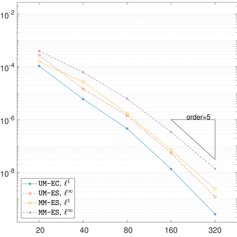
Refer to caption
Refer to caption
Figure 5.1: Example 5.1. The errors and convergence orders in velocity u2subscript𝑢2u_{2} at t=0.1𝑡0.1t=0.1 obtained by our schemes. left: the two-layer case, right: the three-layer case.
Example 5.2 (1D WB test).

This example is used to verify the WB properties of our schemes for the 1D ML-SWEs. The physical domain is [0,20]020[0,20] with outflow boundary conditions, and the bottom topography is a smooth Gaussian profile

b(x)=2e(x9)2/2+3e(x11.5)2,𝑏𝑥2superscript𝑒superscript𝑥9223superscript𝑒superscript𝑥11.52b(x)=2e^{-(x-9)^{2}/2}+3e^{-(x-11.5)^{2}}, (5.4)

or a discontinuous square step

b(x)={2,ifx[9,13],0,otherwise.𝑏𝑥cases2if𝑥9130otherwiseb(x)=\begin{cases}2,~{}&\text{if}\quad x\in[9,13],\\ 0,~{}&\text{otherwise}.\end{cases} (5.5)

The initial data are h1=6h2bsubscript16subscript2𝑏h_{1}=6-h_{2}-b, h2=4bsubscript24𝑏h_{2}=4-b for the two-layer case with the density ratio r12=4/5subscript𝑟1245r_{12}=4/5, ρ2=1subscript𝜌21\rho_{2}=1, while h1=8h2h3bsubscript18subscript2subscript3𝑏h_{1}=8-h_{2}-h_{3}-b, h2=6h3bsubscript26subscript3𝑏h_{2}=6-h_{3}-b, h3=4bsubscript34𝑏h_{3}=4-b for the three-layer case with r12=4/5subscript𝑟1245r_{12}=4/5, r13=2/3subscript𝑟1323r_{13}=2/3, r23=5/6subscript𝑟2356r_{23}=5/6, ρ3=6/5subscript𝜌365\rho_{3}=6/5. The velocities are zero, and the problem is simulated up to t=0.2𝑡0.2t=0.2 with the gravitational acceleration constant taken as g=1𝑔1g=1. The monitor function is the same as that in Example 5.1, but with θ=100𝜃100\theta=100, and σ=h2𝜎subscript2\sigma=h_{2}, h3subscript3h_{3} for the two-layer and three-layer cases, respectively.

Tables 5.1-5.2 give the 1superscript1\ell^{1} and superscript\ell^{\infty} errors in h1+h2+bsubscript1subscript2𝑏h_{1}+h_{2}+b and h2+bsubscript2𝑏h_{2}+b for the two-layer case, and the errors in h1+h2+h3+bsubscript1subscript2subscript3𝑏h_{1}+h_{2}+h_{3}+b, h2+h3+bsubscript2subscript3𝑏h_{2}+h_{3}+b, and h3+bsubscript3𝑏h_{3}+b for the three-layer case with 50 mesh points, respectively. The errors are all at the level of rounding error in double precision, showing that our schemes are WB. The water surface levels, bottom topography b𝑏b, and the mesh trajectories are plotted in Figures 5.2-5.3. One can observe that our schemes can preserve the lake at rest well, and the mesh points concentrate near the sharp transitions of the bottom topography.

UM-ES MM-ES
1superscript1\ell^{1} error superscript\ell^{\infty} error 1superscript1\ell^{1} error superscript\ell^{\infty} error
b𝑏b in (5.4) h1+h2+bsubscript1subscript2𝑏h_{1}+h_{2}+b 9.95e-15 2.66e-15 3.02e-14 5.33e-15
h2+bsubscript2𝑏h_{2}+b 1.03e-14 3.55e-15 2.50e-14 3.55e-15
b𝑏b in (5.5) h1+h2+bsubscript1subscript2𝑏h_{1}+h_{2}+b 2.13e-15 1.78e-15 3.91e-14 4.44e-15
h2+bsubscript2𝑏h_{2}+b 1.07e-15 1.78e-15 3.80e-14 5.33e-15
Table 5.1: Example 5.2 for the two-layer case. Errors in the water surface levels obtained by using our schemes with 505050 mesh points at t=0.2𝑡0.2t=0.2, with the bottom topography (5.4) and (5.5).
UM-ES MM-ES
1superscript1\ell^{1} error superscript\ell^{\infty} error 1superscript1\ell^{1} error superscript\ell^{\infty} error
b𝑏b in (5.4) h1+h2+h3+bsubscript1subscript2subscript3𝑏h_{1}+h_{2}+h_{3}+b 1.99e-14 3.55e-15 7.03e-14 1.07e-14
h2+h3+bsubscript2subscript3𝑏h_{2}+h_{3}+b 2.31e-14 3.55e-15 5.97e-14 1.07e-14
h3+bsubscript3𝑏h_{3}+b 1.76e-14 3.55e-15 5.05e-14 8.88e-15
b𝑏b in (5.5) h1+h2+h3+bsubscript1subscript2subscript3𝑏h_{1}+h_{2}+h_{3}+b 4.62e-15 1.78e-15 4.90e-14 8.88e-15
h2+h3+bsubscript2subscript3𝑏h_{2}+h_{3}+b 5.33e-15 2.67e-15 5.29e-14 7.11e-15
h3+bsubscript3𝑏h_{3}+b 8.88e-15 3.55e-15 4.67e-14 7.11e-15
Table 5.2: Example 5.2 for the three-layer case. Errors in the water surface levels obtained by using our schemes with 505050 mesh points at t=0.2𝑡0.2t=0.2, with the bottom topography (5.4) and (5.5).
Refer to caption
Refer to caption
Refer to caption
Refer to caption
Figure 5.2: Example 5.2 for the two-layer case. Left: the mesh trajectories obtained by the MM-ES scheme, right: the bottom topography b𝑏b and water surface levels. Top: with the bottom topography (5.4), bottom: with the bottom topography (5.5). The results are obtained with 505050 mesh points at t=0.2𝑡0.2t=0.2.
Refer to caption
Refer to caption
Refer to caption
Refer to caption
Figure 5.3: Example 5.2 for the three-layer case. Left: the mesh trajectories obtained by the MM-ES scheme, right: the bottom topography b𝑏b and water surface levels. Top: with the bottom topography (5.4), bottom: with the bottom topography (5.5). The results are obtained with 505050 mesh points at t=0.2𝑡0.2t=0.2.
Example 5.3 (1D dam break over a flat bottom).

This test investigates the ability of the proposed schemes to capture the small-scale wave structures. The initial data for the two-layer case are

h2(x,0)subscript2𝑥0\displaystyle h_{2}(x,0) ={0.6,ifx5,0.4,otherwise,absentcases0.6if𝑥50.4otherwise\displaystyle=\begin{cases}0.6,&\text{if}\quad x\leqslant 5,\\ 0.4,&\text{otherwise},\\ \end{cases}
h1(x,0)subscript1𝑥0\displaystyle h_{1}(x,0) =1h2(x,0),absent1subscript2𝑥0\displaystyle=1-h_{2}(x,0),

with zero velocities in the physical domain [0,10]010[0,10] and r12=0.8subscript𝑟120.8r_{12}=0.8, ρ2=1subscript𝜌21\rho_{2}=1. The output time is t=1.25𝑡1.25t=1.25 and outflow boundary conditions are used. For the three-layer case, the initial data for the water depth are

h3(x,0)subscript3𝑥0\displaystyle h_{3}(x,0) ={0.6,ifx5,0.4,otherwise,absentcases0.6if𝑥50.4otherwise\displaystyle=\begin{cases}0.6,&\text{if}\quad x\leqslant 5,\\ 0.4,&\text{otherwise},\\ \end{cases}
h2(x,0)subscript2𝑥0\displaystyle h_{2}(x,0) =1h3(x,0),absent1subscript3𝑥0\displaystyle=1-h_{3}(x,0),
h1(x,0)subscript1𝑥0\displaystyle h_{1}(x,0) =2h2(x,0)h3(x,0),absent2subscript2𝑥0subscript3𝑥0\displaystyle=2-h_{2}(x,0)-h_{3}(x,0),

with the density ratios r12=0.8subscript𝑟120.8r_{12}=0.8, r13=0.64subscript𝑟130.64r_{13}=0.64, r23=0.8subscript𝑟230.8r_{23}=0.8, ρ3=1.0subscript𝜌31.0\rho_{3}=1.0, and the output time t=0.8𝑡0.8t=0.8. The gravitational acceleration constant is g=9.812𝑔9.812g=9.812 in both cases. The monitor function is chosen as that in Example 5.2, but with θ=100𝜃100\theta=100, and σ=h1+h2+b𝜎subscript1subscript2𝑏\sigma=h_{1}+h_{2}+b and h1+h2+h3+bsubscript1subscript2subscript3𝑏h_{1}+h_{2}+h_{3}+b for the two-layer and three-layer cases, respectively.

Figure 5.4 shows the mesh trajectories and water surface levels h1+h2+bsubscript1subscript2𝑏h_{1}+h_{2}+b and h2+bsubscript2𝑏h_{2}+b obtained by the UM-ES and MM-ES schemes for the two-layer case at t=1.25𝑡1.25t=1.25, and corresponding results for the three-layer case at t=0.8𝑡0.8t=0.8. The reference solutions are given by using the UM-ES schemes with 300030003000 mesh points. One can see that the wave structures for the three-layer case are more complicated, and our schemes can well capture the discontinuities without obvious oscillations. Moreover, the MM-ES scheme using 400400400 mesh points gives similar local resolution compared to the UM-ES scheme using 120012001200 mesh points, which indicates the high efficiency of our schemes on adaptive moving meshes. Figure 5.5 gives the evolution of the discrete total energy iJiη(𝑼i)Δξsubscript𝑖subscript𝐽𝑖𝜂subscript𝑼𝑖Δ𝜉\sum\limits_{i}J_{i}\eta(\bm{U}_{i})\Delta\xi obtained by the MM-ES scheme with 400400400 mesh points in both cases, which decay as expected.
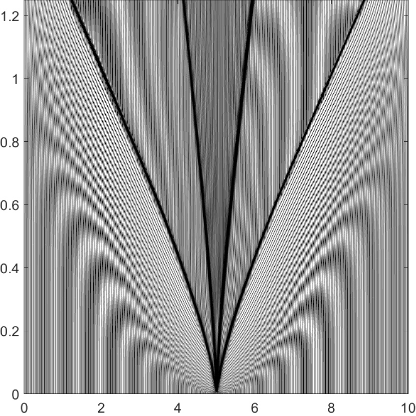
Refer to caption
(a) mesh trajectory
Refer to caption
(b) h1+h2+bsubscript1subscript2𝑏h_{1}+h_{2}+b
Refer to caption
(c) h2+bsubscript2𝑏h_{2}+b
Refer to caption
(d) mesh trajectory
Refer to caption
(e) h1+h2+h3+bsubscript1subscript2subscript3𝑏h_{1}+h_{2}+h_{3}+b
Refer to caption
(f) h3+bsubscript3𝑏h_{3}+b
Figure 5.4: Example 5.3. The numerical solutions obtained by the UM-ES and MM-ES schemes, the reference solutions are obtained by using the UM-ES schemes with 300030003000 mesh points. Top: the two-layer case, bottom: the three-layer case.
Refer to caption
(a) two-layer case
Refer to caption
(b) three-layer case
Figure 5.5: Example 5.3. The evolution of the discrete total energy by using the MM-ES scheme with 400 mesh points.
Example 5.4 (Small perturbation test).

To test the ability of our schemes to capture small perturbations in the steady-state flow, the bottom topography consisting of a “hump” [32] is considered here

b(x)={0.25(cos(10π(x0.5))+1)2,if0.4x0.6,0,otherwise,𝑏𝑥cases0.2510𝜋𝑥0.512if0.4𝑥0.60otherwiseb(x)=\begin{cases}0.25(\cos(10\pi(x-0.5))+1)-2,&\text{if}\quad 0.4\leqslant x\leqslant 0.6,\\ 0,&\text{otherwise},\end{cases}

and the initial data for the two-layer case are

h1subscript1\displaystyle h_{1} ={1.00001,if0.1x0.2,1,otherwise,absentcases1.00001if0.1𝑥0.21otherwise\displaystyle=\begin{cases}1.00001,&\text{if}\quad 0.1\leqslant x\leqslant 0.2,\\ 1,&\text{otherwise},\\ \end{cases}
h2subscript2\displaystyle h_{2} =1b,absent1𝑏\displaystyle=-1-b,

with initial zero velocities and g=9.812𝑔9.812g=9.812, r12=0.98subscript𝑟120.98r_{12}=0.98, ρ2=1subscript𝜌21\rho_{2}=1. The physical domain is taken as [1,1]11[-1,1] with outflow boundary conditions. For the three-layer case, the initial data are

h1subscript1\displaystyle h_{1} =1,absent1\displaystyle=1,
h2subscript2\displaystyle h_{2} ={1.00001,if0.1x0.2,1,otherwise,absentcases1.00001if0.1𝑥0.21otherwise\displaystyle=\begin{cases}1.00001,&\text{if}\quad 0.1\leqslant x\leqslant 0.2,\\ 1,&\text{otherwise},\\ \end{cases}
h3subscript3\displaystyle h_{3} =1b,absent1𝑏\displaystyle=-1-b,

with zero velocities, and r12=0.9898subscript𝑟120.9898r_{12}=0.9898, r23=0.98subscript𝑟230.98r_{23}=0.98, r13=0.97subscript𝑟130.97r_{13}=0.97, ρ3=1.0subscript𝜌31.0\rho_{3}=1.0. The monitor function is the same as Example 5.3.

Figure 5.6 presents the numerical solutions obtained by the UM-ES and MM-ES schemes with 200200200 and 600600600 mesh points at t=0.15𝑡0.15t=0.15 for the two-layer case, and at t=0.1𝑡0.1t=0.1 for the three-layer case, respectively. The reference solutions are obtained by the UM-ES scheme with 300030003000 mesh points. It can be seen that the structures in the solution can be captured well and there is no apparent numerical oscillation. The results obtained by using the adaptive moving mesh are better than those on the fixed uniform mesh with the same number of mesh points, and comparable to those on the fixed uniform mesh with three times the number of mesh points. Figure 5.7 gives the discrete total energy evolution versus time obtained by the MM-ES scheme with 200200200 mesh points, which decays as expected.
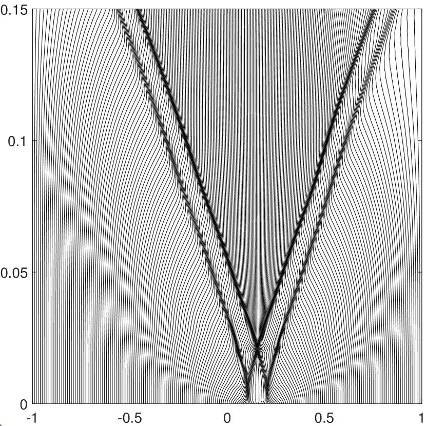
Refer to caption
(a) mesh trajectory
Refer to caption
(b) h1+h2+bsubscript1subscript2𝑏h_{1}+h_{2}+b
Refer to caption
(c) u1subscript𝑢1u_{1}
Refer to caption
(d) mesh trajectory
Refer to caption
(e) h1+h2+bsubscript1subscript2𝑏h_{1}+h_{2}+b
Refer to caption
(f) u1subscript𝑢1u_{1}
Figure 5.6: Example 5.4. The mesh trajectories and numerical solutions obtained by using the UM-ES and MM-ES schemes at t=0.15𝑡0.15t=0.15 for the two-layer case (top), and at t=0.1𝑡0.1t=0.1 for the three-layer case (bottom). The reference solutions are obtained by using the UM-ES scheme with 300030003000 mesh points.
Refer to caption
(a) two-layer case
Refer to caption
(b) three-layer case
Figure 5.7: Example 5.4. The evolution of the discrete total energy over time by using the MM-ES schemes with 200200200 mesh points.

5.3 2D tests

Example 5.5 (Accuracy test with manufactured solutions).

This test is taken to verify the accuracy of the 2D schemes. The manufactured solutions are constructed for the two-layer and three-layer SWEs with extra source terms. For the two-layer case, the exact solutions are

h1(x1,x2,t)=cos(πt)cos(πx1)+cos(πt)cos(πx2)+6,subscript1subscript𝑥1subscript𝑥2𝑡𝜋𝑡𝜋subscript𝑥1𝜋𝑡𝜋subscript𝑥26\displaystyle h_{1}(x_{1},x_{2},t)=\cos\left(\pi t\right)\cos\left(\pi x_{1}\right)+\cos\left(\pi t\right)\cos\left(\pi x_{2}\right)+6,
u1(x1,x2,t)=sin(πt)sin(πx1)h1,v1(x1,x2,t)=sin(πt)sin(πx2)h1,formulae-sequencesubscript𝑢1subscript𝑥1subscript𝑥2𝑡𝜋𝑡𝜋subscript𝑥1subscript1subscript𝑣1subscript𝑥1subscript𝑥2𝑡𝜋𝑡𝜋subscript𝑥2subscript1\displaystyle u_{1}(x_{1},x_{2},t)=\frac{\sin\left(\pi t\right)\sin\left(\pi x_{1}\right)}{h_{1}},~{}v_{1}(x_{1},x_{2},t)=\frac{\sin\left(\pi t\right)\sin\left(\pi x_{2}\right)}{h_{1}},
h2(x1,x2,t)=cos(πt)cos(πx1)+cos(πt)cos(πx2)+4,subscript2subscript𝑥1subscript𝑥2𝑡𝜋𝑡𝜋subscript𝑥1𝜋𝑡𝜋subscript𝑥24\displaystyle h_{2}(x_{1},x_{2},t)=\cos\left(\pi t\right)\cos\left(\pi x_{1}\right)+\cos\left(\pi t\right)\cos\left(\pi x_{2}\right)+4,
u2(x1,x2,t)=sin(πt)sin(πx1)h2,v2(x1,x2,t)=sin(πt)sin(πx2)h2,formulae-sequencesubscript𝑢2subscript𝑥1subscript𝑥2𝑡𝜋𝑡𝜋subscript𝑥1subscript2subscript𝑣2subscript𝑥1subscript𝑥2𝑡𝜋𝑡𝜋subscript𝑥2subscript2\displaystyle u_{2}(x_{1},x_{2},t)=\frac{\sin\left(\pi t\right)\sin\left(\pi x_{1}\right)}{h_{2}},~{}v_{2}(x_{1},x_{2},t)=\frac{\sin\left(\pi t\right)\sin\left(\pi x_{2}\right)}{h_{2}},
b(x1,x2)=sin(πx1)+sin(πx1)+32,𝑏subscript𝑥1subscript𝑥2𝜋subscript𝑥1𝜋subscript𝑥132\displaystyle b(x_{1},x_{2})=\sin\left(\pi x_{1}\right)+\sin\left(\pi x_{1}\right)+\frac{3}{2},

and the source terms are omitted here. The physical domain is [0,2]×[0,2]0202[0,2]\times[0,2] with periodic boundary conditions, and the output time is t=0.1𝑡0.1t=0.1. The density ratio r12subscript𝑟12r_{12} is 7/107107/10, ρ2=1subscript𝜌21\rho_{2}=1 with the gravitational acceleration constant g=1𝑔1g=1. For the three-layer case, the exact solutions can be constructed similarly, presented in B, with r12=7/10subscript𝑟12710r_{12}=7/10, r13=7/13subscript𝑟13713r_{13}=7/13, r23=10/13subscript𝑟231013r_{23}=10/13, ρ3=13/10subscript𝜌31310\rho_{3}=13/10. The monitor function is chosen as

ω=(1+θ(|𝝃σ|max|𝝃σ|)2)12,𝜔superscript1𝜃superscriptsubscript𝝃𝜎subscript𝝃𝜎212\omega=\left(1+\theta\left(\frac{\left|\nabla_{\bm{\xi}}\sigma\right|}{\max\left|\nabla_{\bm{\xi}}\sigma\right|}\right)^{2}\right)^{\frac{1}{2}},

where θ=1𝜃1\theta=1 and σ=h2+b𝜎subscript2𝑏\sigma=h_{2}+b for both cases.

Figure 5.8 gives the 1superscript1\ell^{1} and superscript\ell^{\infty} errors and corresponding convergence orders of the UM-ES and MM-ES schemes in velocity u2subscript𝑢2u_{2} at t=0.1𝑡0.1t=0.1, which verify the 555th-order accuracy. Figure 5.9 shows the water surface levels and bottom topography obtained by the UM-ES scheme with 160×160160160160\times 160 mesh, and the evolution of the discrete total energy i,jη(𝑼i,j)Δx1Δx2subscript𝑖𝑗𝜂subscript𝑼𝑖𝑗Δsubscript𝑥1Δsubscript𝑥2\sum\limits_{i,j}\eta(\bm{U}_{i,j})\Delta x_{1}\Delta x_{2}, which decays on different meshes.
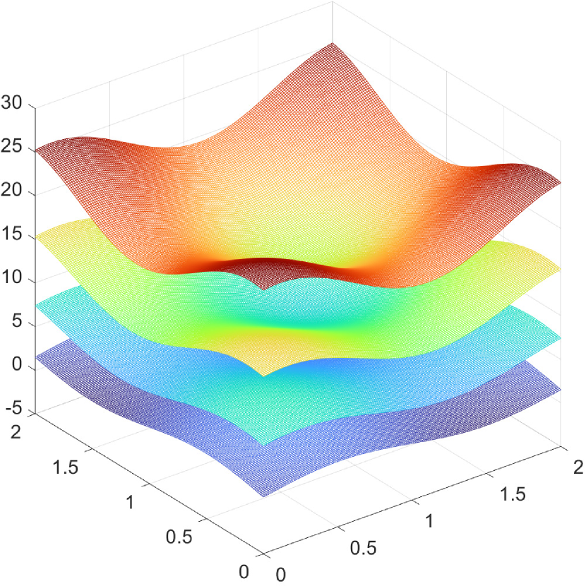
Refer to caption
(a) two-layer case
Refer to caption
(b) three-layer case
Figure 5.8: Example 5.5. The errors and convergence rates in u2subscript𝑢2u_{2} at t=0.1𝑡0.1t=0.1.
Refer to caption
(a) h1+h2+bsubscript1subscript2𝑏h_{1}+h_{2}+b, h2+bsubscript2𝑏h_{2}+b, and b𝑏b
Refer to caption
(b) discrete total energy
Refer to caption
(c) h1+h2+h3+bsubscript1subscript2subscript3𝑏h_{1}+h_{2}+h_{3}+b, h2+h3+bsubscript2subscript3𝑏h_{2}+h_{3}+b, h3+bsubscript3𝑏h_{3}+b, and b𝑏b
Refer to caption
(d) discrete total energy
Figure 5.9: Example 5.5. The water surface levels and bottom topography obtained by using the UM-ES scheme with 160×160160160160\times 160 mesh at t=0.1𝑡0.1t=0.1, and the discrete total energy evolution over time on different meshes. Top: two-layer case, bottom: three-layer case.
Example 5.6 (Accuracy test with a moving vortex).

This example is used to further test the accuracy of our MM-ES schemes for the two-layer SWEs. Similar to [20, 51], a moving vortex can be constructed as follows

h1=5,u1=v1=0,formulae-sequencesubscript15subscript𝑢1subscript𝑣10\displaystyle h_{1}=5,~{}u_{1}=v_{1}=0,
h2=1umax2e1R2/(2g),subscript21superscriptsubscript𝑢2superscript𝑒1superscript𝑅22𝑔\displaystyle h_{2}=1-u_{\max}^{2}e^{1-R^{2}}/(2g),
(u2,v2)=(1,1)+umaxe0.5(1R2)((x2t),x1t),subscript𝑢2subscript𝑣211subscript𝑢superscript𝑒0.51superscript𝑅2subscript𝑥2𝑡subscript𝑥1𝑡\displaystyle\left(u_{2},v_{2}\right)=(1,1)+u_{\max}e^{0.5\left(1-R^{2}\right)}(-(x_{2}-t),~{}x_{1}-t),

with umax=0.2subscript𝑢0.2u_{\max}=0.2, R=(x1t)2+(x2t)2𝑅superscriptsubscript𝑥1𝑡2superscriptsubscript𝑥2𝑡2R=\sqrt{(x_{1}-t)^{2}+(x_{2}-t)^{2}}, g=1𝑔1g=1, r12=0.7subscript𝑟120.7r_{12}=0.7, ρ2=1subscript𝜌21\rho_{2}=1, flat bottom topography, and the extra source terms

𝑺=(0,exp(1(tx2)2(tx1)2)(2t2x1)40,exp(1(tx2)2(tx1)2)(2t2x2)40,0,0,0,0)T.𝑺superscript01superscript𝑡subscript𝑥22superscript𝑡subscript𝑥122𝑡2subscript𝑥1401superscript𝑡subscript𝑥22superscript𝑡subscript𝑥122𝑡2subscript𝑥2400000T\bm{S}=(0,~{}-\frac{\exp(1-(t-x_{2})^{2}-(t-x_{1})^{2})(2t-2x_{1})}{40},~{}-\frac{\exp(1-(t-x_{2})^{2}-(t-x_{1})^{2})(2t-2x_{2})}{40},~{}0,~{}0,~{}0,~{}0)^{\mathrm{T}}.

The monitor function is set to be

ω=(1+10(|𝝃(h2+b)|max|𝝃(h2+b)|)2+10(|Δ𝝃(h2+b)|max|Δ𝝃(h2+b)|)2)12.𝜔superscript110superscriptsubscript𝝃subscript2𝑏subscript𝝃subscript2𝑏210superscriptsubscriptΔ𝝃subscript2𝑏subscriptΔ𝝃subscript2𝑏212\omega=\left({1+10\left(\frac{|\nabla_{\bm{\xi}}(h_{2}+b)|}{\max|\nabla_{\bm{\xi}}(h_{2}+b)|}\right)^{2}+10\left(\frac{|\Delta_{\bm{\xi}}(h_{2}+b)|}{\max|\Delta_{\bm{\xi}}(h_{2}+b)|}\right)^{2}}\right)^{\frac{1}{2}}.

Figure 5.10 shows the adaptive mesh, the errors, and convergence orders in the water depth h2subscript2h_{2} at t=0.5𝑡0.5t=0.5, and the evolution of the discrete total energy. It is seen that the 555th-order accuracy is achieved with the mesh points adaptively concentrating near the moving vortex, and the discrete total energy i,jJi,jη(𝑼i,j)Δξ1Δξ2subscript𝑖𝑗subscript𝐽𝑖𝑗𝜂subscript𝑼𝑖𝑗Δsubscript𝜉1Δsubscript𝜉2\sum\limits_{i,j}J_{i,j}\eta(\bm{U}_{i,j})\Delta\xi_{1}\Delta{\xi_{2}} decays as expected.

Refer to caption
(a) adaptive mesh
Refer to caption
(b) errors and convergence orders
Refer to caption
(c) discrete total energy
Figure 5.10: Example 5.6. The 80×80808080\times 80 adaptive mesh with 555 equally spaced contour lines of the water surface h2+bsubscript2𝑏h_{2}+b, the errors and convergence orders in h2+bsubscript2𝑏h_{2}+b at t=0.5𝑡0.5t=0.5, and the discrete total energy obtained by the MM-ES scheme with 80×80808080\times 80 mesh.
Example 5.7 (2D WB test).

The example is utilized to verify the WB properties of our 2D UM-ES and MM-ES schemes. The bottom topography is

b(x1,x2)=1.2exp(50((x10.5)2+(x20.5)2)),(x1,x2)[0,1]×[0,1],formulae-sequence𝑏subscript𝑥1subscript𝑥21.250superscriptsubscript𝑥10.52superscriptsubscript𝑥20.52subscript𝑥1subscript𝑥20101b(x_{1},x_{2})=1.2\exp\left(-50\left((x_{1}-0.5)^{2}+(x_{2}-0.5)^{2}\right)\right),~{}(x_{1},x_{2})\in[0,1]\times[0,1], (5.6)

or

b(x1,x2)={1.0,if(x1,x2)[0.4,0.5]×[0.4,0.5],0.5,if(x1,x2)([0.4,0.6]×[0.4,0.6])([0.3,0.5]×[0.3,0.5])\([0.4,0.5]×[0.4,0.5]),0,otherwise.𝑏subscript𝑥1subscript𝑥2cases1.0ifsubscript𝑥1subscript𝑥20.40.50.40.50.5ifsubscript𝑥1subscript𝑥20.40.60.40.6\0.30.50.30.50.40.50.40.50otherwiseb(x_{1},x_{2})=\begin{cases}1.0,&\text{if}\quad(x_{1},x_{2})\in[0.4,0.5]\times[0.4,0.5],\\ 0.5,&\text{if}\quad(x_{1},x_{2})\in([0.4,0.6]\times[0.4,0.6])\cup([0.3,0.5]\times[0.3,0.5])\backslash([0.4,0.5]\times[0.4,0.5]),\\ 0,&\text{otherwise}.\end{cases} (5.7)

For the two-layer case, the initial data are h2=2bsubscript22𝑏h_{2}=2-b, h1=2.2h2bsubscript12.2subscript2𝑏h_{1}=2.2-h_{2}-b, zero velocities, with g=1𝑔1g=1, r12=4/5subscript𝑟1245r_{12}=4/5, ρ2=1subscript𝜌21\rho_{2}=1. For the three-layer case, the initial data are h3=2bsubscript32𝑏h_{3}=2-b, h2=2.2h2bsubscript22.2subscript2𝑏h_{2}=2.2-h_{2}-b, h1=2.4h2h1bsubscript12.4subscript2subscript1𝑏h_{1}=2.4-h_{2}-h_{1}-b with r12=4/5subscript𝑟1245r_{12}=4/5, r13=2/3subscript𝑟1323r_{13}=2/3, r23=5/6subscript𝑟2356r_{23}=5/6, ρ3=6/5subscript𝜌365\rho_{3}=6/5. The monitor function is chosen as

ω=(1+θ(|𝝃σ|max|𝝃σ|)2)12,𝜔superscript1𝜃superscriptsubscript𝝃𝜎subscript𝝃𝜎212\omega=\left(1+\theta\left(\frac{\left|\nabla_{\bm{\xi}}\sigma\right|}{\max\left|\nabla_{\bm{\xi}}\sigma\right|}\right)^{2}\right)^{\frac{1}{2}},

with θ=100𝜃100\theta=100, σ=h2𝜎subscript2\sigma=h_{2} and σ=h3𝜎subscript3\sigma=h_{3} for the two-layer and three-layer cases, respectively.

The 1superscript1\ell^{1} and superscript\ell^{\infty} errors in the water surface levels are listed in Tables 5.3-5.4 by using our schemes with 100×100100100100\times 100 mesh at t=0.1𝑡0.1t=0.1, from which one observes that the lake at rest is maintained up to the rounding error in double precision. Figures 5.11-5.12 show the results of the water surface levels h1+h2+bsubscript1subscript2𝑏h_{1}+h_{2}+b, h2+bsubscript2𝑏h_{2}+b and h1+h2+h3+bsubscript1subscript2subscript3𝑏h_{1}+h_{2}+h_{3}+b, h1+h2+bsubscript1subscript2𝑏h_{1}+h_{2}+b, h2+bsubscript2𝑏h_{2}+b with corresponding bottom topography b𝑏b obtained by using the MM-ES scheme with 100×100100100100\times 100 mesh. Those results confirm that our schemes are WB on both fixed and adaptive moving meshes.

UM-ES MM-ES
1superscript1\ell^{1} error superscript\ell^{\infty} error 1superscript1\ell^{1} error superscript\ell^{\infty} error
b𝑏b in (5.6) h1+h2+bsubscript1subscript2𝑏h_{1}+h_{2}+b 6.32e-16 3.11e-15 1.02e-15 1.73e-14
h2+bsubscript2𝑏h_{2}+b 6.40e-16 3.55e-15 9.24e-16 1.42e-14
b𝑏b in (5.7) h1+h2+bsubscript1subscript2𝑏h_{1}+h_{2}+b 1.95e-18 8.88e-16 1.99e-15 2.27e-14
h2+bsubscript2𝑏h_{2}+b 2.13e-18 8.88e-16 1.83e-15 1.84e-14
Table 5.3: Example 5.7 for the two-layer case. Errors in h1+h2+bsubscript1subscript2𝑏h_{1}+h_{2}+b and h2+bsubscript2𝑏h_{2}+b obtained by our schemes using 100×100100100100\times 100 mesh at t=0.1𝑡0.1t=0.1, with the bottom topography (5.6) and (5.7).
UM-ES MM-ES
1superscript1\ell^{1} error superscript\ell^{\infty} error 1superscript1\ell^{1} error superscript\ell^{\infty} error
b𝑏b in (5.6) h1+h2+h3+bsubscript1subscript2subscript3𝑏h_{1}+h_{2}+h_{3}+b 2.81e-16 2.67e-15 1.17e-15 1.24e-14
h2+h3+bsubscript2subscript3𝑏h_{2}+h_{3}+b 3.86e-16 3.11e-15 1.13e-15 1.07e-14
h3+bsubscript3𝑏h_{3}+b 3.11e-16 2.44e-15 1.02e-15 9.33e-15
b𝑏b in (5.7) h1+h2+h3+bsubscript1subscript2subscript3𝑏h_{1}+h_{2}+h_{3}+b 2.66e-16 8.88e-16 1.57e-15 9.77e-15
h2+h3+bsubscript2subscript3𝑏h_{2}+h_{3}+b 2.63e-16 1.33e-15 1.51e-15 1.11e-14
h3+bsubscript3𝑏h_{3}+b 1.99e-16 2.22e-15 1.41e-15 1.29e-14
Table 5.4: Example 5.7 for the three-layer case. Errors in h1+h2+h3+bsubscript1subscript2subscript3𝑏h_{1}+h_{2}+h_{3}+b, h2+h3+bsubscript2subscript3𝑏h_{2}+h_{3}+b and h3+bsubscript3𝑏h_{3}+b obtained by our schemes using 100×100100100100\times 100 mesh at t=0.1𝑡0.1t=0.1, with the bottom topography (5.6) and (5.7).
Refer to caption
(a) adaptive mesh
Refer to caption
(b) water surface levels
Refer to caption
(c) adaptive mesh
Refer to caption
(d) water surface levels
Figure 5.11: Example 5.7 for the two-layer case. The water surface levels h1+h2+bsubscript1subscript2𝑏h_{1}+h_{2}+b and h2+bsubscript2𝑏h_{2}+b with the bottom topography b𝑏b and adaptive meshes obtained by using the MM-ES scheme with 100×100100100100\times 100 mesh at t=0.1𝑡0.1t=0.1. Top: with the bottom topography (5.6), bottom: with the bottom topography (5.7).
Refer to caption
(a) adaptive mesh
Refer to caption
(b) water surface levels
Refer to caption
(c) adaptive mesh
Refer to caption
(d) water surface levels
Figure 5.12: Example 5.7 for the three-layer case. The water surface levels h1+h2+h3+bsubscript1subscript2subscript3𝑏h_{1}+h_{2}+h_{3}+b, h2+h3+bsubscript2subscript3𝑏h_{2}+h_{3}+b, h3+bsubscript3𝑏h_{3}+b, with the bottom topography b𝑏b and adaptive meshes obtained by using the MM-ES scheme with 100×100100100100\times 100 mesh at t=0.1𝑡0.1t=0.1. Top: with the bottom topography (5.6), bottom: with the bottom topography (5.7).
Example 5.8 (Propagation of an interface over a non-flat bottom).

This example tests the interface propagation over a non-flat bottom topography. Initially, the bottom topography is a Gaussian-shaped function

b(x1,x2)=0.05e100(x12+x22)1,𝑏subscript𝑥1subscript𝑥20.05superscript𝑒100superscriptsubscript𝑥12superscriptsubscript𝑥221b(x_{1},~{}x_{2})=0.05e^{-100\left(x_{1}^{2}+x_{2}^{2}\right)}-1,

with the initial data for the two-layer case

(h1,u1,v1,h2,u2,v2)={(0.50,2.5,2.5,0.50b,2.5,2.5),if(x1,x2)Ω,(0.45,2.5,2.5,0.45b,2.5,2.5),otherwise,subscript1subscript𝑢1subscript𝑣1subscript2subscript𝑢2subscript𝑣2cases0.502.52.50.50𝑏2.52.5ifsubscript𝑥1subscript𝑥2Ω0.452.52.50.45𝑏2.52.5otherwise\left(h_{1},~{}u_{1},~{}v_{1},~{}h_{2},~{}u_{2},~{}v_{2}\right)=\begin{cases}\left(0.50,~{}2.5,~{}2.5,~{}-0.50-b,~{}2.5,~{}2.5\right),&\text{if}\quad\left(x_{1},x_{2}\right)\in\Omega,\\ \left(0.45,~{}2.5,~{}2.5,~{}-0.45-b,~{}2.5,~{}2.5\right),&\text{otherwise},\end{cases}

where

Ω=Ωabsent\displaystyle\Omega= {(x1,x2)x1<0.5,x2<0}{(x1,x2)x1<0,x2<0.5}conditional-setsubscript𝑥1subscript𝑥2formulae-sequencesubscript𝑥10.5subscript𝑥20conditional-setsubscript𝑥1subscript𝑥2formulae-sequencesubscript𝑥10subscript𝑥20.5\displaystyle\{(x_{1},x_{2})\mid x_{1}<-0.5,~{}x_{2}<0\}\cup\{(x_{1},x_{2})\mid x_{1}<0,~{}x_{2}<-0.5\}
{(x1,x2)(x1+0.5)2+(x2+0.5)2<0.52}.conditional-setsubscript𝑥1subscript𝑥2superscriptsubscript𝑥10.52superscriptsubscript𝑥20.52superscript0.52\displaystyle\cup\{(x_{1},x_{2})\mid(x_{1}+0.5)^{2}+(x_{2}+0.5)^{2}<0.5^{2}\}.

The physical domain is [1,1]×[1,1]1111[-1,1]\times[-1,1] with outflow boundary conditions, and g=10𝑔10g=10, r12=49/50subscript𝑟124950r_{12}=49/50, ρ2=1subscript𝜌21\rho_{2}=1. The solution is evolved up to t=0.1𝑡0.1t=0.1. For the three-layer case, the initial data are

(h2,u2,v2,h3,u3,v3)={(0.50,2.5,2.5,0.50b,2.5,2.5),if(x1,x2)Ω,(0.45,2.5,2.5,0.45b,2.5,2.5),otherwise,subscript2subscript𝑢2subscript𝑣2subscript3subscript𝑢3subscript𝑣3cases0.502.52.50.50𝑏2.52.5ifsubscript𝑥1subscript𝑥2Ω0.452.52.50.45𝑏2.52.5otherwise\displaystyle\left(h_{2},~{}u_{2},~{}v_{2},~{}h_{3},~{}u_{3},~{}v_{3}\right)=\begin{cases}\left(0.50,~{}2.5,~{}2.5,~{}-0.50-b,~{}2.5,~{}2.5\right),&\text{if}\quad\left(x_{1},~{}x_{2}\right)\in\Omega,\\ \left(0.45,~{}2.5,~{}2.5,~{}-0.45-b,~{}2.5,~{}2.5\right),&\text{otherwise},\end{cases}
(h1,u1,v1)=(1.0,0.0,0.0),subscript1subscript𝑢1subscript𝑣11.00.00.0\displaystyle\left(h_{1},~{}u_{1},~{}v_{1}\right)=\left(1.0,~{}0.0,~{}0.0\right),

with r12=49/50subscript𝑟124950r_{12}=49/50, r13=49/55subscript𝑟134955r_{13}=49/55, r23=10/11subscript𝑟231011r_{23}=10/11, and ρ3=11/10subscript𝜌31110\rho_{3}=11/10. The monitor function is the same as that in Example 5.7, except for σ=h1𝜎subscript1\sigma=h_{1} in both cases and θ=300𝜃300\theta=300.

Refer to caption
(a) two-layer case
Refer to caption
(b) three-layer case
Figure 5.13: Example 5.8. The 200×200200200200\times 200 adaptive meshes obtained by the MM-ES scheme.
Refer to caption
(a) h1+h2+bsubscript1subscript2𝑏h_{1}+h_{2}+b
Refer to caption
(b) h1subscript1h_{1}
Refer to caption
(c) h1+h2+bsubscript1subscript2𝑏h_{1}+h_{2}+b
Refer to caption
(d) h1subscript1h_{1}
Refer to caption
(e) h1+h2+bsubscript1subscript2𝑏h_{1}+h_{2}+b
Refer to caption
(f) h1subscript1h_{1}
Figure 5.14: Example 5.8 for the two-layer case. 303030 equally spaced contours obtained by our schemes. From top to bottom: MM-ES (200×200)200200(200\times 200), UM-ES (200×200)200200(200\times 200), UM-ES (600×600)600600(600\times 600).
Refer to caption
(a) h1+h2+h3+bsubscript1subscript2subscript3𝑏h_{1}+h_{2}+h_{3}+b
Refer to caption
(b) h1subscript1h_{1}
Refer to caption
(c) h1+h2+h3+bsubscript1subscript2subscript3𝑏h_{1}+h_{2}+h_{3}+b
Refer to caption
(d) h1subscript1h_{1}
Refer to caption
(e) h1+h2+h3+bsubscript1subscript2subscript3𝑏h_{1}+h_{2}+h_{3}+b
Refer to caption
(f) h1subscript1h_{1}
Figure 5.15: Example 5.8 for the three-layer case. 303030 equally spaced contours obtained by our schemes. From top to bottom: MM-ES (200×\times200), UM-ES (200×\times200), UM-ES (600×\times600).
two-layer three-layer
UM-ES (200×200200200200\times 200) 3m44s 21m29s
MM-ES (200×200200200200\times 200) 20m05s 63m35s
UM-ES (600×600600600600\times 600) 2h42m 17h54m
Table 5.5: Example 5.8. The CPU times for our schemes on the different meshes. The tests are solved up to t=0.1𝑡0.1t=0.1.

Figure 5.13 shows the 200×200200200200\times 200 adaptive meshes obtained by the MM-ES schemes. Figure 5.14 plots 303030 equally spaced contours of the water surface levels obtained by the UM-ES scheme on 200×200200200200\times 200 and 600×600600600600\times 600 meshes, and obtained by the MM-ES scheme with 200×200200200200\times 200 mesh at t=0.1𝑡0.1t=0.1. It can be seen that the results are comparable to those in [30], and our schemes can capture the complicated structure around (0.2,0.2)0.20.2(0.2,~{}0.2) without oscillations. One can observe that the mesh points concentrate near the sharp transitions of the water surface level h1subscript1h_{1}, which improves the local resolution such that the results on 200×200200200200\times 200 adaptive moving mesh are as good as those on 600×600600600600\times 600 fixed uniform mesh. The numerical results for the three-layer case are also shown in Figure 5.15. One can also see that the resolution of the numerical results obtained by the MM-ES scheme is better than that obtained by the UM-ES scheme with the same number of mesh points.

To verify the high efficiency of our schemes on adaptive moving meshes, the CPU times are listed in Table 5.5. One observes that the MM-ES scheme takes less CPU time compared with the UM-ES scheme using a finer mesh, which illustrates the efficiency of our adaptive moving mesh method. The CPU times are tested with the code programmed by MATLAB R2021b on a laptop with Intel® Core™ i7-8750H CPU @2.20GHz, 24GB memory.

Example 5.9 (Circle dam-break problem).

This example test is taken from [13], which is used to verify the shock-capturing ability and efficiency of our schemes for the two-layer SWEs. The bottom topography is

b(x1,x2)=0.5e5(x12+x22)2.0,𝑏subscript𝑥1subscript𝑥20.5superscript𝑒5superscriptsubscript𝑥12superscriptsubscript𝑥222.0b(x_{1},x_{2})=0.5e^{-5\left(x_{1}^{2}+x_{2}^{2}\right)}-2.0,

and the initial data are

h1(x1,x2,0)={1.8,ifx12+x221,0.2,otherwise,subscript1subscript𝑥1subscript𝑥20cases1.8ifsuperscriptsubscript𝑥12superscriptsubscript𝑥2210.2otherwise\displaystyle h_{1}(x_{1},x_{2},0)=\begin{cases}1.8,&\text{if}\quad x_{1}^{2}+x_{2}^{2}\geqslant 1,\\ 0.2,&\text{otherwise},\end{cases}
h2(x1,x2,0)={0.20.5e5(x12+x22),ifx12+x221,1.80.5e5(x12+x22),otherwise,subscript2subscript𝑥1subscript𝑥20cases0.20.5superscript𝑒5superscriptsubscript𝑥12superscriptsubscript𝑥22ifsuperscriptsubscript𝑥12superscriptsubscript𝑥2211.80.5superscript𝑒5superscriptsubscript𝑥12superscriptsubscript𝑥22otherwise\displaystyle h_{2}(x_{1},x_{2},0)=\begin{cases}0.2-0.5e^{-5\left(x_{1}^{2}+x_{2}^{2}\right)},&\text{if}\quad x_{1}^{2}+x_{2}^{2}\geqslant 1,\\ 1.8-0.5e^{-5\left(x_{1}^{2}+x_{2}^{2}\right)},&\text{otherwise},\end{cases}

with zero velocities in the physical domain [2,2]×[2,2]2222[-2,2]\times[-2,2] with outflow boundary conditions, and g=9.812𝑔9.812g=9.812, r12=0.98subscript𝑟120.98r_{12}=0.98, ρ2=1subscript𝜌21\rho_{2}=1. The output time is t=1.0𝑡1.0t=1.0. The monitor function is the same as that in Example 5.7, but with σ=h2+b+5𝜎subscript2𝑏5\sigma=h_{2}+b+5.

Refer to caption
(a) adaptive mesh
Refer to caption
(b) 404040 contours of h2+bsubscript2𝑏h_{2}+b
Refer to caption
(c) cut line along x2=0subscript𝑥20x_{2}=0
Figure 5.16: Example 5.9. The numerical results obtained by using the MM-ES scheme with 150×150150150150\times 150 mesh, and the UM-ES scheme with 150×150150150150\times 150 and 600×600600600600\times 600 meshes.

Figure 5.16 gives the 150×150150150150\times 150 adaptive mesh, the 404040 equally spaced contours of the water surface level h2+bsubscript2𝑏h_{2}+b obtained by the MM-ES scheme on 150×150150150150\times 150 mesh and the cut line along x2=0subscript𝑥20x_{2}=0 of h2+bsubscript2𝑏h_{2}+b compared with the UM-ES scheme. The reference solution is obtained by using the UM-ES scheme with 1000×1000100010001000\times 1000 mesh. It is seen that our schemes can capture the discontinuities accurately and the MM-ES scheme gives a higher resolution around x1±1.7subscript𝑥1plus-or-minus1.7x_{1}\approx\pm 1.7 compared with the UM-ES scheme on a finer mesh.

Example 5.10 (The perturbed flow in lake at rest).

This example tests the ability of our schemes to capture small perturbations over the lake at rest for the two-layer SWEs. The physical domain is [0,2]×[0,1]0201[0,2]\times[0,1] with outflow boundary conditions. The bottom topography resembles an “oval hump”, similar to the example for the single-layer SWEs in [46, 47], but with extra water depth h1subscript1h_{1}. Initially,

h2={1.01b,ifx1[0.05,0.15],1b,otherwise,subscript2cases1.01𝑏ifsubscript𝑥10.050.151𝑏otherwise\displaystyle h_{2}=\begin{cases}1.01-b,~{}&\text{if}\quad x_{1}\in[0.05,0.15],\\ 1-b,~{}&\text{otherwise},\end{cases}
b=0.8exp(5(x10.9)250(x20.5)2),𝑏0.85superscriptsubscript𝑥10.9250superscriptsubscript𝑥20.52\displaystyle b=0.8\exp(-5(x_{1}-0.9)^{2}-50(x_{2}-0.5)^{2}),
h1=2h2b,subscript12subscript2𝑏\displaystyle h_{1}=2-h_{2}-b,
u1=v1=0,u2=v2=0.formulae-sequencesubscript𝑢1subscript𝑣10subscript𝑢2subscript𝑣20\displaystyle u_{1}=v_{1}=0,~{}u_{2}=v_{2}=0.

The density ratio is r12=0.85subscript𝑟120.85r_{12}=0.85, with ρ2=1.0subscript𝜌21.0\rho_{2}=1.0. The monitor function used in this test is the same as Example 5.7, except that the value of σ𝜎\sigma is equal to h2+bsubscript2𝑏h_{2}+b.

Figure 5.17 shows the 303030 equally spaced contour lines of the water surface levels h1+h2+bsubscript1subscript2𝑏h_{1}+h_{2}+b and h2+bsubscript2𝑏h_{2}+b at t=0.9𝑡0.9t=0.9, 1.31.31.3, 1.71.71.7, 2.02.02.0 obtained by using the UM-ES scheme with 300×150300150300\times 150 mesh. The 300×150300150300\times 150 adaptive mesh obtained by the MM-ES schemes at t=0.9𝑡0.9t=0.9 is plotted in Figure 5.18. The comparison of the results between the UM-ES and MM-ES schemes is shown in Figure 5.19. One observes that our schemes can capture the wave structures accurately without obvious oscillations, and results of the MM-ES scheme on the 300×150300150300\times 150 mesh are comparable to those of the UM-ES scheme on the 600×300600300600\times 300 mesh, highlighting the efficiency of the MM-ES schemes.

Refer to caption
Refer to caption
Refer to caption
Refer to caption
Refer to caption
Refer to caption
Refer to caption
Refer to caption
Figure 5.17: Example 5.10. 303030 equally spaced contours of the water surface levels obtained by the UM-ES scheme on 300×150300150300\times 150 mesh. From top to bottom: t=0.9𝑡0.9t=0.9, 1.31.31.3, 1.71.71.7, 2.02.02.0. Left: h1+h2+bsubscript1subscript2𝑏h_{1}+h_{2}+b, right: h2+bsubscript2𝑏h_{2}+b.
Refer to caption
Figure 5.18: Example 5.10. The adaptive mesh obtained by the MM-ES scheme with 300×150300150300\times 150 mesh at t=0.9𝑡0.9t=0.9.
Refer to caption
Refer to caption
Refer to caption
Refer to caption
Refer to caption
Refer to caption
Figure 5.19: Example 5.10. 303030 equally spaced contours of the water surface levels obtained by the UM-ES and MM-ES schemes at t=0.9𝑡0.9t=0.9. From top to bottom: MM-ES (300×\times150), UM-ES (300×\times150), UM-ES (600×\times300). Left: h1+h2+bsubscript1subscript2𝑏h_{1}+h_{2}+b, right: h2+bsubscript2𝑏h_{2}+b.

6 Conclusion

This paper has presented high-order accurate WB ES finite difference schemes for the ML-SWEs (the number of layers M2𝑀2M\geqslant 2) with non-flat bottom topography on fixed and adaptive moving meshes, which extended our previous works [20, 51]. The proof of the convexity of the energy function for an arbitrary M𝑀M was more challenging than the single-layer case due to the coupling terms resulting from the multiple layers in the energy function, leading to the more complicated Hessian matrix. The recurrence relations of the leading principal minors or the quadratic forms of the Hessian matrix were found to complete the proof. To design WB schemes, the sufficient condition for the EC fluxes should include compatible discretizations of the source terms similar to the single-layer case. The condition was decoupled into M𝑀M individual equalities for each layer, so that it was convenient to construct the two-point EC flux for the multi-layer system. The high-order WB EC fluxes were constructed by using the two-point WB EC flux as a building block, and then the high-order WB ES schemes satisfying semi-discrete energy inequalities were obtained by adding the WENO-based dissipation terms to the high-order WB EC fluxes with compatible discretizations of the source terms. The high-order explicit SSP-RK3 schemes were used to obtain the fully-discrete schemes, which were proved to preserve the lake at rest. Moreover, the extension to the adaptive moving meshes was built on the reformulated system and carefully designed dissipation terms, extending the techniques proposed in [51]. Some two- and three-layer test cases were employed in the numerical experiments to confirm our findings, and due to the lack of an analytical expression for the eigenstructure of the multi-layer system, the proper amount of dissipation was chosen by the estimation of the maximal wave speed, employing the method in [30].

Acknowledgments

The authors were partially supported by the National Key R&D Program of China (Project Number 2020YFA0712000), the National Natural Science Foundation of China (No. 12171227 & 12288101). J.M. Duan was supported by the Alexander von Humboldt Foundation Research Fellowship CHN-1234352-HFST-P.

Appendix A Proof of the convexity by using quadratic forms

Under the condition 0<ρ1<ρ2<<ρ𝒩<0subscript𝜌1subscript𝜌2subscript𝜌𝒩0<\rho_{1}<\rho_{2}<\dots<\rho_{\mathcal{N}}<\dots, the quadratic form of the Hessian matrix 𝒩=2η/𝑼2subscript𝒩superscript2𝜂superscript𝑼2\mathcal{M}_{\mathcal{N}}=\partial^{2}{\eta}/\partial{\bm{U}}^{2} is

Q𝒩:=𝜷𝒩𝒩𝜷𝒩T=assignsubscript𝑄𝒩subscript𝜷𝒩subscript𝒩superscriptsubscript𝜷𝒩Tabsent\displaystyle Q_{\mathcal{N}}:=\bm{\beta}_{\mathcal{N}}\mathcal{M}_{\mathcal{N}}\bm{\beta}_{\mathcal{N}}^{\mathrm{T}}= gρ1(m=1𝒩β3m2)2+gm=2𝒩(ρmρm1)(l=m𝒩β3l2)2𝑔subscript𝜌1superscriptsuperscriptsubscript𝑚1𝒩subscript𝛽3𝑚22𝑔superscriptsubscript𝑚2𝒩subscript𝜌𝑚subscript𝜌𝑚1superscriptsuperscriptsubscript𝑙𝑚𝒩subscript𝛽3𝑙22\displaystyle\ g\rho_{1}\left(\sum_{m=1}^{\mathcal{N}}\beta_{3m-2}\right)^{2}+g\sum_{m=2}^{\mathcal{N}}(\rho_{m}-\rho_{m-1})\left(\sum_{l=m}^{\mathcal{N}}\beta_{3l-2}\right)^{2} (A.1)
+m=1𝒩ρmhm((umβ3m2β3m1)2+(vmβ3m2β3m)2),superscriptsubscript𝑚1𝒩subscript𝜌𝑚subscript𝑚superscriptsubscript𝑢𝑚subscript𝛽3𝑚2subscript𝛽3𝑚12superscriptsubscript𝑣𝑚subscript𝛽3𝑚2subscript𝛽3𝑚2\displaystyle+\sum_{m=1}^{\mathcal{N}}\dfrac{\rho_{m}}{h_{m}}\left(\left(u_{m}\beta_{3m-2}-\beta_{3m-1}\right)^{2}+\left(v_{m}\beta_{3m-2}-\beta_{3m}\right)^{2}\right),

with 𝜷𝒩=(β1,,β3𝒩)1×3𝒩subscript𝜷𝒩subscript𝛽1subscript𝛽3𝒩superscript13𝒩\bm{\beta}_{\mathcal{N}}=\left(\beta_{1},\dots,\beta_{3\mathcal{N}}\right)\in\mathbb{R}^{1\times{3\mathcal{N}}}, thus the energy function is convex.

Proof.

The proof is given by induction on 𝒩𝒩\mathcal{N}. When 𝒩=2𝒩2\mathcal{N}=2, it is easy to show that the quadratic form of the Hessian matrix 2subscript2\mathcal{M}_{2} (2.5) is

Q2=subscript𝑄2absent\displaystyle Q_{2}= ρ1h1(u12β12u1β1β2+β22+v12β12v1β1β3+β32)subscript𝜌1subscript1superscriptsubscript𝑢12subscript𝛽12subscript𝑢1subscript𝛽1subscript𝛽2superscriptsubscript𝛽22superscriptsubscript𝑣12subscript𝛽12subscript𝑣1subscript𝛽1subscript𝛽3superscriptsubscript𝛽32\displaystyle\ \dfrac{\rho_{1}}{h_{1}}\left(u_{1}^{2}\beta_{1}-2u_{1}\beta_{1}\beta_{2}+\beta_{2}^{2}+v_{1}^{2}\beta_{1}-2v_{1}\beta_{1}\beta_{3}+\beta_{3}^{2}\right)
+ρ2h2(u22β42u2β4β5+β52+v22β42v2β4β6+β62)subscript𝜌2subscript2superscriptsubscript𝑢22subscript𝛽42subscript𝑢2subscript𝛽4subscript𝛽5superscriptsubscript𝛽52superscriptsubscript𝑣22subscript𝛽42subscript𝑣2subscript𝛽4subscript𝛽6superscriptsubscript𝛽62\displaystyle+\dfrac{\rho_{2}}{h_{2}}\left(u_{2}^{2}\beta_{4}-2u_{2}\beta_{4}\beta_{5}+\beta_{5}^{2}+v_{2}^{2}\beta_{4}-2v_{2}\beta_{4}\beta_{6}+\beta_{6}^{2}\right)
+gρ1β12+2gρ1β1β4+gρ2β42𝑔subscript𝜌1superscriptsubscript𝛽122𝑔subscript𝜌1subscript𝛽1subscript𝛽4𝑔subscript𝜌2superscriptsubscript𝛽42\displaystyle+g\rho_{1}\beta_{1}^{2}+2g\rho_{1}\beta_{1}\beta_{4}+g\rho_{2}\beta_{4}^{2}
=\displaystyle= ρ1h1((u1β1β2)2+(v1β1β3)2)+ρ2h2((u2β4β5)2+(v2β4β6)2)subscript𝜌1subscript1superscriptsubscript𝑢1subscript𝛽1subscript𝛽22superscriptsubscript𝑣1subscript𝛽1subscript𝛽32subscript𝜌2subscript2superscriptsubscript𝑢2subscript𝛽4subscript𝛽52superscriptsubscript𝑣2subscript𝛽4subscript𝛽62\displaystyle\ \dfrac{\rho_{1}}{h_{1}}\left(\left(u_{1}\beta_{1}-\beta_{2}\right)^{2}+\left(v_{1}\beta_{1}-\beta_{3}\right)^{2}\right)+\dfrac{\rho_{2}}{h_{2}}\left(\left(u_{2}\beta_{4}-\beta_{5}\right)^{2}+\left(v_{2}\beta_{4}-\beta_{6}\right)^{2}\right)
+gρ1(β1+β4)2+g(ρ2ρ1)β42,𝑔subscript𝜌1superscriptsubscript𝛽1subscript𝛽42𝑔subscript𝜌2subscript𝜌1superscriptsubscript𝛽42\displaystyle+g\rho_{1}\left(\beta_{1}+\beta_{4}\right)^{2}+g\left(\rho_{2}-\rho_{1}\right)\beta_{4}^{2},

which is positive as 0<ρ1<ρ20subscript𝜌1subscript𝜌20<\rho_{1}<\rho_{2} for any 𝜷26\{𝟎6}subscript𝜷2\superscript6subscript06\bm{\beta}_{2}\in\mathbb{R}^{6}\backslash\{\bm{0}_{6}\}, thus the matrix 2subscript2\mathcal{M}_{2} is positive-definite.

Now it suffices to show that if the quadratic form of 𝒩subscript𝒩\mathcal{M}_{\mathcal{N}} is Q𝒩subscript𝑄𝒩Q_{\mathcal{N}} in (A.1), then the the quadratic form of 𝒩+1subscript𝒩1\mathcal{M}_{\mathcal{N}+1} is Q𝒩+1subscript𝑄𝒩1Q_{\mathcal{N}+1}. According to the matrix structure in Lemma 2.1, one can calculate Q𝒩+1subscript𝑄𝒩1Q_{\mathcal{N}+1} by adding several extra terms to Q𝒩subscript𝑄𝒩Q_{\mathcal{N}}, which can be written as

Q𝒩+1=subscript𝑄𝒩1absent\displaystyle Q_{\mathcal{N}+1}= 𝜷𝒩+1𝒩+1𝜷𝒩+1Tsubscript𝜷𝒩1subscript𝒩1superscriptsubscript𝜷𝒩1T\displaystyle\ \bm{\beta}_{\mathcal{N}+1}\mathcal{M}_{\mathcal{N}+1}\bm{\beta}_{\mathcal{N}+1}^{\mathrm{T}}
=\displaystyle= Q𝒩+2β3𝒩+1(m=1𝒩gρmβ3m2)+gρ𝒩+1β3𝒩+12subscript𝑄𝒩2subscript𝛽3𝒩1superscriptsubscript𝑚1𝒩𝑔subscript𝜌𝑚subscript𝛽3𝑚2𝑔subscript𝜌𝒩1superscriptsubscript𝛽3𝒩12\displaystyle\ Q_{\mathcal{N}}+2\beta_{3\mathcal{N}+1}\left(\sum_{m=1}^{\mathcal{N}}g\rho_{m}\beta_{3m-2}\right)+g\rho_{\mathcal{N}+1}\beta_{3\mathcal{N}+1}^{2}
+ρ𝒩+1h𝒩+1((u𝒩+1β3𝒩+1β3𝒩+2)2+(v𝒩+1β3𝒩+1β3𝒩+3)2)subscript𝜌𝒩1subscript𝒩1superscriptsubscript𝑢𝒩1subscript𝛽3𝒩1subscript𝛽3𝒩22superscriptsubscript𝑣𝒩1subscript𝛽3𝒩1subscript𝛽3𝒩32\displaystyle+\dfrac{\rho_{\mathcal{N}+1}}{h_{\mathcal{N}+1}}\left(\left(u_{\mathcal{N}+1}\beta_{3\mathcal{N}+1}-\beta_{3\mathcal{N}+2}\right)^{2}+\left(v_{\mathcal{N}+1}\beta_{3\mathcal{N}+1}-\beta_{3\mathcal{N}+3}\right)^{2}\right)
=\displaystyle= gρ1(m=1𝒩β3m2)2+gm=2𝒩(ρmρm1)(l=m𝒩β3l2)2𝑔subscript𝜌1superscriptsuperscriptsubscript𝑚1𝒩subscript𝛽3𝑚22𝑔superscriptsubscript𝑚2𝒩subscript𝜌𝑚subscript𝜌𝑚1superscriptsuperscriptsubscript𝑙𝑚𝒩subscript𝛽3𝑙22\displaystyle\ g\rho_{1}\left(\sum_{m=1}^{\mathcal{N}}\beta_{3m-2}\right)^{2}+g\sum_{m=2}^{\mathcal{N}}(\rho_{m}-\rho_{m-1})\left(\sum_{l=m}^{\mathcal{N}}\beta_{3l-2}\right)^{2}
+m=1𝒩ρmhm((umβ3m2β3m1)2+(vmβ3m2β3m)2)superscriptsubscript𝑚1𝒩subscript𝜌𝑚subscript𝑚superscriptsubscript𝑢𝑚subscript𝛽3𝑚2subscript𝛽3𝑚12superscriptsubscript𝑣𝑚subscript𝛽3𝑚2subscript𝛽3𝑚2\displaystyle+\sum_{m=1}^{\mathcal{N}}\dfrac{\rho_{m}}{h_{m}}\left(\left(u_{m}\beta_{3m-2}-\beta_{3m-1}\right)^{2}+\left(v_{m}\beta_{3m-2}-\beta_{3m}\right)^{2}\right)
+2β3𝒩+1(m=1𝒩gρmβ3m2)+gρ𝒩+1β3𝒩+122subscript𝛽3𝒩1superscriptsubscript𝑚1𝒩𝑔subscript𝜌𝑚subscript𝛽3𝑚2𝑔subscript𝜌𝒩1superscriptsubscript𝛽3𝒩12\displaystyle+2\beta_{3\mathcal{N}+1}\left(\sum_{m=1}^{\mathcal{N}}g\rho_{m}\beta_{3m-2}\right)+g\rho_{\mathcal{N}+1}\beta_{3\mathcal{N}+1}^{2}
+ρ𝒩+1h𝒩+1((u𝒩+1β3𝒩+1β3𝒩+2)2+(v𝒩+1β3𝒩+1β3𝒩+3)2)subscript𝜌𝒩1subscript𝒩1superscriptsubscript𝑢𝒩1subscript𝛽3𝒩1subscript𝛽3𝒩22superscriptsubscript𝑣𝒩1subscript𝛽3𝒩1subscript𝛽3𝒩32\displaystyle+\dfrac{\rho_{\mathcal{N}+1}}{h_{\mathcal{N}+1}}\left(\left(u_{\mathcal{N}+1}\beta_{3\mathcal{N}+1}-\beta_{3\mathcal{N}+2}\right)^{2}+\left(v_{\mathcal{N}+1}\beta_{3\mathcal{N}+1}-\beta_{3\mathcal{N}+3}\right)^{2}\right)
=:absent:\displaystyle=: 1+2,subscript1subscript2\displaystyle\ \mathcal{H}_{1}+\mathcal{H}_{2},

with

1=m=1𝒩+1ρmhm((umβ3m2β3m1)2+(vmβ3m2β3m)2),subscript1superscriptsubscript𝑚1𝒩1subscript𝜌𝑚subscript𝑚superscriptsubscript𝑢𝑚subscript𝛽3𝑚2subscript𝛽3𝑚12superscriptsubscript𝑣𝑚subscript𝛽3𝑚2subscript𝛽3𝑚2\displaystyle\mathcal{H}_{1}=\sum_{m=1}^{\mathcal{N}+1}\dfrac{\rho_{m}}{h_{m}}\left(\left(u_{m}\beta_{3m-2}-\beta_{3m-1}\right)^{2}+\left(v_{m}\beta_{3m-2}-\beta_{3m}\right)^{2}\right),
2=gρ1(m=1𝒩β3m2)2+gm=2𝒩(ρmρm1)(l=m𝒩β3l2)2subscript2𝑔subscript𝜌1superscriptsuperscriptsubscript𝑚1𝒩subscript𝛽3𝑚22𝑔superscriptsubscript𝑚2𝒩subscript𝜌𝑚subscript𝜌𝑚1superscriptsuperscriptsubscript𝑙𝑚𝒩subscript𝛽3𝑙22\displaystyle\mathcal{H}_{2}=g\rho_{1}\left(\sum_{m=1}^{\mathcal{N}}\beta_{3m-2}\right)^{2}+g\sum_{m=2}^{\mathcal{N}}(\rho_{m}-\rho_{m-1})\left(\sum_{l=m}^{\mathcal{N}}\beta_{3l-2}\right)^{2}
+2β3𝒩+1(m=1𝒩gρmβ3m2)+gρ𝒩+1β3𝒩+12.2subscript𝛽3𝒩1superscriptsubscript𝑚1𝒩𝑔subscript𝜌𝑚subscript𝛽3𝑚2𝑔subscript𝜌𝒩1superscriptsubscript𝛽3𝒩12\displaystyle\quad\quad+2\beta_{3\mathcal{N}+1}\left(\sum_{m=1}^{\mathcal{N}}g\rho_{m}\beta_{3m-2}\right)+g\rho_{\mathcal{N}+1}\beta_{3\mathcal{N}+1}^{2}.

The term 2subscript2\mathcal{H}_{2} can be further simplified as

2=subscript2absent\displaystyle\mathcal{H}_{2}= gρ1((m=1𝒩β3m2)2+2β3𝒩+1(m=1𝒩β3m2)+β3𝒩+12)𝑔subscript𝜌1superscriptsuperscriptsubscript𝑚1𝒩subscript𝛽3𝑚222subscript𝛽3𝒩1superscriptsubscript𝑚1𝒩subscript𝛽3𝑚2superscriptsubscript𝛽3𝒩12\displaystyle\ g\rho_{1}\left(\left(\sum_{m=1}^{\mathcal{N}}\beta_{3m-2}\right)^{2}+2\beta_{3\mathcal{N}+1}\left(\sum_{m=1}^{\mathcal{N}}\beta_{3m-2}\right)+\beta_{3\mathcal{N}+1}^{2}\right)
+gm=2𝒩(ρmρm1)((l=m𝒩β3l2)2+2β3𝒩+1(l=m𝒩β3l2)+β3𝒩+12)𝑔superscriptsubscript𝑚2𝒩subscript𝜌𝑚subscript𝜌𝑚1superscriptsuperscriptsubscript𝑙𝑚𝒩subscript𝛽3𝑙222subscript𝛽3𝒩1superscriptsubscript𝑙𝑚𝒩subscript𝛽3𝑙2superscriptsubscript𝛽3𝒩12\displaystyle+g\sum_{m=2}^{\mathcal{N}}\left(\rho_{m}-\rho_{m-1}\right)\left(\left(\sum_{l=m}^{\mathcal{N}}\beta_{3l-2}\right)^{2}+2\beta_{3\mathcal{N}+1}\left(\sum_{l=m}^{\mathcal{N}}\beta_{3l-2}\right)+\beta_{3\mathcal{N}+1}^{2}\right)
+2gβ3𝒩+1(m=1𝒩ρmβ3m2)+gρ𝒩+1β3𝒩+122𝑔subscript𝛽3𝒩1superscriptsubscript𝑚1𝒩subscript𝜌𝑚subscript𝛽3𝑚2𝑔subscript𝜌𝒩1superscriptsubscript𝛽3𝒩12\displaystyle+2g\beta_{3\mathcal{N}+1}\left(\sum_{m=1}^{\mathcal{N}}\rho_{m}\beta_{3m-2}\right)+g\rho_{\mathcal{N}+1}\beta_{3\mathcal{N}+1}^{2}
2gβ3𝒩+1(ρ1(m=1𝒩β3m2)+m=2𝒩(ρmρm1)(l=m𝒩β3l2))2𝑔subscript𝛽3𝒩1subscript𝜌1superscriptsubscript𝑚1𝒩subscript𝛽3𝑚2superscriptsubscript𝑚2𝒩subscript𝜌𝑚subscript𝜌𝑚1superscriptsubscript𝑙𝑚𝒩subscript𝛽3𝑙2\displaystyle-2g\beta_{3\mathcal{N}+1}\left(\rho_{1}\left(\sum_{m=1}^{\mathcal{N}}\beta_{3m-2}\right)+\sum_{m=2}^{\mathcal{N}}\left(\rho_{m}-\rho_{m-1}\right)\left(\sum_{l=m}^{\mathcal{N}}\beta_{3l-2}\right)\right)
gβ3𝒩+12(ρ1+m=2𝒩(ρmρm1)).𝑔superscriptsubscript𝛽3𝒩12subscript𝜌1superscriptsubscript𝑚2𝒩subscript𝜌𝑚subscript𝜌𝑚1\displaystyle-g\beta_{3\mathcal{N}+1}^{2}\left(\rho_{1}+\sum_{m=2}^{\mathcal{N}}\left(\rho_{m}-\rho_{m-1}\right)\right).

Using

gρ𝒩+1β3𝒩+12gβ3𝒩+12(ρ1+m=2𝒩(ρmρm1))=g(ρ𝒩+1ρ𝒩)β3𝒩+12,𝑔subscript𝜌𝒩1superscriptsubscript𝛽3𝒩12𝑔superscriptsubscript𝛽3𝒩12subscript𝜌1superscriptsubscript𝑚2𝒩subscript𝜌𝑚subscript𝜌𝑚1𝑔subscript𝜌𝒩1subscript𝜌𝒩superscriptsubscript𝛽3𝒩12\displaystyle g\rho_{\mathcal{N}+1}\beta_{3\mathcal{N}+1}^{2}-g\beta_{3\mathcal{N}+1}^{2}\left(\rho_{1}+\sum_{m=2}^{\mathcal{N}}\left(\rho_{m}-\rho_{m-1}\right)\right)=g\left(\rho_{\mathcal{N}+1}-\rho_{\mathcal{N}}\right)\beta_{3\mathcal{N}+1}^{2},
ρ1(m=1𝒩β3m2)+m=2𝒩(ρmρm1)(l=m𝒩β3l2)=m=1𝒩ρmβ3m2,subscript𝜌1superscriptsubscript𝑚1𝒩subscript𝛽3𝑚2superscriptsubscript𝑚2𝒩subscript𝜌𝑚subscript𝜌𝑚1superscriptsubscript𝑙𝑚𝒩subscript𝛽3𝑙2superscriptsubscript𝑚1𝒩subscript𝜌𝑚subscript𝛽3𝑚2\displaystyle\rho_{1}\left(\sum_{m=1}^{\mathcal{N}}\beta_{3m-2}\right)+\sum_{m=2}^{\mathcal{N}}\left(\rho_{m}-\rho_{m-1}\right)\left(\sum_{l=m}^{\mathcal{N}}\beta_{3l-2}\right)=\sum_{m=1}^{\mathcal{N}}\rho_{m}\beta_{3m-2},

yields

2=gρ1(m=1𝒩+1β3m2)2+gm=2𝒩+1(ρmρm1)(l=m𝒩+1β3l2)2.subscript2𝑔subscript𝜌1superscriptsuperscriptsubscript𝑚1𝒩1subscript𝛽3𝑚22𝑔superscriptsubscript𝑚2𝒩1subscript𝜌𝑚subscript𝜌𝑚1superscriptsuperscriptsubscript𝑙𝑚𝒩1subscript𝛽3𝑙22\displaystyle\mathcal{H}_{2}=g\rho_{1}\left(\sum_{m=1}^{\mathcal{N}+1}\beta_{3m-2}\right)^{2}+g\sum_{m=2}^{\mathcal{N}+1}(\rho_{m}-\rho_{m-1})\left(\sum_{l=m}^{\mathcal{N}+1}\beta_{3l-2}\right)^{2}.

Thus the quadratic form of 𝒩+1subscript𝒩1\mathcal{M}_{\mathcal{N}+1} is Q𝒩+1subscript𝑄𝒩1Q_{\mathcal{N}+1}. Moreover, it is easy to verify that Q𝒩>0subscript𝑄𝒩0Q_{\mathcal{N}}>0, so the energy function is convex. The proof is completed. ∎

Appendix B Explicit expressions of the exact solutions used in Examples 5.1, 5.5

In Example 5.1, the source terms for the two-layer case are 𝑺=(0,s2,0,s4,0)T𝑺superscript0subscript𝑠20subscript𝑠40T\bm{S}=(0,s_{2},0,s_{4},0)^{\mathrm{T}}, with

s2=subscript𝑠2absent\displaystyle s_{2}= πcos(πx)(cos(πt)cos(πx)+6)+πcos(πt)sin(πx)𝜋𝜋𝑥𝜋𝑡𝜋𝑥6𝜋𝜋𝑡𝜋𝑥\displaystyle~{}\pi\cos\left(\pi x\right)\left(\cos\left(\pi t\right)\cos\left(\pi x\right)+6\right)+\pi\cos\left(\pi t\right)\sin\left(\pi x\right)
3πcos(πt)sin(πx)(cos(πt)cos(πx)+6)2πcos(πt)sin(πx)(cos(πt)cos(πx)2+3)3𝜋𝜋𝑡𝜋𝑥𝜋𝑡𝜋𝑥62𝜋𝜋𝑡𝜋𝑥𝜋𝑡𝜋𝑥23\displaystyle~{}-\frac{3\pi\cos\left(\pi t\right)\sin\left(\pi x\right)\left(\cos\left(\pi t\right)\cos\left(\pi x\right)+6\right)}{2}-\pi\cos\left(\pi t\right)\sin\left(\pi x\right)\left(\frac{\cos\left(\pi t\right)\cos\left(\pi x\right)}{2}+3\right)
+πcos(πt)sin(πt)2sin(πx)3(cos(πt)cos(πx)+6)2+2πcos(πx)sin(πt)2sin(πx)cos(πt)cos(πx)+6,\displaystyle~{}+\frac{\pi\cos\left(\pi t\right){\sin\left(\pi t\right)}^{2}{\sin\left(\pi x\right)}^{3}}{{\left(\cos\left(\pi t\right)\cos\left(\pi x\right)+6\right)}^{2}}+\frac{2\pi\cos\left(\pi x\right){\sin\left(\pi t\right)}^{2}\sin\left(\pi x\right)}{\cos\left(\pi t\right)\cos\left(\pi x\right)+6},
s4=subscript𝑠4absent\displaystyle s_{4}= πcos(πx)(cos(πt)cos(πx)+4)+πcos(πt)sin(πx)𝜋𝜋𝑥𝜋𝑡𝜋𝑥4𝜋𝜋𝑡𝜋𝑥\displaystyle~{}\pi\cos\left(\pi x\right)\left(\cos\left(\pi t\right)\cos\left(\pi x\right)+4\right)+\pi\cos\left(\pi t\right)\sin\left(\pi x\right)
πcos(πt)sin(πx)(cos(πt)cos(πx)+4)2𝜋𝜋𝑡𝜋𝑥𝜋𝑡𝜋𝑥42\displaystyle-\frac{\pi\cos\left(\pi t\right)\sin\left(\pi x\right)\left(\cos\left(\pi t\right)\cos\left(\pi x\right)+4\right)}{2}
πcos(πt)sin(πx)(cos(πt)cos(πx)2+2)πrcos(πt)sin(πx)(cos(πt)cos(πx)+4)𝜋𝜋𝑡𝜋𝑥𝜋𝑡𝜋𝑥22𝜋𝑟𝜋𝑡𝜋𝑥𝜋𝑡𝜋𝑥4\displaystyle~{}-\pi\cos\left(\pi t\right)\sin\left(\pi x\right)\left(\frac{\cos\left(\pi t\right)\cos\left(\pi x\right)}{2}+2\right)-\pi r\cos\left(\pi t\right)\sin\left(\pi x\right)\left(\cos\left(\pi t\right)\cos\left(\pi x\right)+4\right)
+πcos(πt)sin(πt)2sin(πx)3(cos(πt)cos(πx)+4)2+2πcos(πx)sin(πt)2sin(πx)cos(πt)cos(πx)+4.\displaystyle~{}+\frac{\pi\cos\left(\pi t\right){\sin\left(\pi t\right)}^{2}{\sin\left(\pi x\right)}^{3}}{{\left(\cos\left(\pi t\right)\cos\left(\pi x\right)+4\right)}^{2}}+\frac{2\pi\cos\left(\pi x\right){\sin\left(\pi t\right)}^{2}\sin\left(\pi x\right)}{\cos\left(\pi t\right)\cos\left(\pi x\right)+4}.

For the three-layer case, the expressions are omitted.

In Example 5.5, the exact solutions for the three-layer case are

h1(x1,x2,t)=cos(πt)cos(πx1)+cos(πt)cos(πx2)+8,subscript1subscript𝑥1subscript𝑥2𝑡𝜋𝑡𝜋subscript𝑥1𝜋𝑡𝜋subscript𝑥28\displaystyle h_{1}(x_{1},x_{2},t)=\cos\left(\pi t\right)\cos\left(\pi x_{1}\right)+\cos\left(\pi t\right)\cos\left(\pi x_{2}\right)+8,
u1(x1,x2,t)=sin(πt)sin(πx1)h1,v1(x1,x2,t)=sin(πt)sin(πx2)h1,formulae-sequencesubscript𝑢1subscript𝑥1subscript𝑥2𝑡𝜋𝑡𝜋subscript𝑥1subscript1subscript𝑣1subscript𝑥1subscript𝑥2𝑡𝜋𝑡𝜋subscript𝑥2subscript1\displaystyle u_{1}(x_{1},x_{2},t)=\frac{\sin\left(\pi t\right)\sin\left(\pi x_{1}\right)}{h_{1}},~{}v_{1}(x_{1},x_{2},t)=\frac{\sin\left(\pi t\right)\sin\left(\pi x_{2}\right)}{h_{1}},
h2(x1,x2,t)=cos(πt)cos(πx1)+cos(πt)cos(πx2)+6,subscript2subscript𝑥1subscript𝑥2𝑡𝜋𝑡𝜋subscript𝑥1𝜋𝑡𝜋subscript𝑥26\displaystyle h_{2}(x_{1},x_{2},t)=\cos\left(\pi t\right)\cos\left(\pi x_{1}\right)+\cos\left(\pi t\right)\cos\left(\pi x_{2}\right)+6,
u2(x1,x2,t)=sin(πt)sin(πx1)h2,v2(x1,x2,t)=sin(πt)sin(πx2)h2,formulae-sequencesubscript𝑢2subscript𝑥1subscript𝑥2𝑡𝜋𝑡𝜋subscript𝑥1subscript2subscript𝑣2subscript𝑥1subscript𝑥2𝑡𝜋𝑡𝜋subscript𝑥2subscript2\displaystyle u_{2}(x_{1},x_{2},t)=\frac{\sin\left(\pi t\right)\sin\left(\pi x_{1}\right)}{h_{2}},~{}v_{2}(x_{1},x_{2},t)=\frac{\sin\left(\pi t\right)\sin\left(\pi x_{2}\right)}{h_{2}},
h3(x1,x2,t)=cos(πt)cos(πx1)+cos(πt)cos(πx2)+4,subscript3subscript𝑥1subscript𝑥2𝑡𝜋𝑡𝜋subscript𝑥1𝜋𝑡𝜋subscript𝑥24\displaystyle h_{3}(x_{1},x_{2},t)=\cos\left(\pi t\right)\cos\left(\pi x_{1}\right)+\cos\left(\pi t\right)\cos\left(\pi x_{2}\right)+4,
u3(x1,x2,t)=sin(πt)sin(πx1)h3,v2(x1,x2,t)=sin(πt)sin(πx2)h3,formulae-sequencesubscript𝑢3subscript𝑥1subscript𝑥2𝑡𝜋𝑡𝜋subscript𝑥1subscript3subscript𝑣2subscript𝑥1subscript𝑥2𝑡𝜋𝑡𝜋subscript𝑥2subscript3\displaystyle u_{3}(x_{1},x_{2},t)=\frac{\sin\left(\pi t\right)\sin\left(\pi x_{1}\right)}{h_{3}},~{}v_{2}(x_{1},x_{2},t)=\frac{\sin\left(\pi t\right)\sin\left(\pi x_{2}\right)}{h_{3}},
b(x1,x2)=sin(πx1)+sin(πx1)+32,𝑏subscript𝑥1subscript𝑥2𝜋subscript𝑥1𝜋subscript𝑥132\displaystyle b(x_{1},x_{2})=\sin\left(\pi x_{1}\right)+\sin\left(\pi x_{1}\right)+\frac{3}{2},

and the extra source terms for the two-layer and three-layer cases can be obtained by some algebraic manipulations similar to Example 5.1.

References

  • [1] R. Abgrall and S. Karni, Two-layer shallow water system: a relaxation approach, SIAM J. Sci. Comput., 31 (2009), 1603–1627.
  • [2] E. Audusse, F. Bouchut, M.O. Bristeau, R. Klein, and B. Perthame, A fast and stable well-balanced scheme with hydrostatic reconstruction for shallow water flows, SIAM J. Sci. Comput., 25 (2004), 2050–2065.
  • [3] A. Bermudez and M.E. Vazquez, Upwind methods for hyperbolic conservation laws with source terms, Computers & Fluids, 23 (1994), 1049–1071.
  • [4] C. Berthon and C. Chalons, A fully well-balanced, positive and entropy-satisfying Godunov-type method for the shallow- water equations, Math. Comp., 85 (2016), 1281–1307.
  • [5] B. Biswas and R.K. Dubey, Low dissipative entropy stable schemes using third order WENO and TVD reconstructions, Adv. Comput. Math., 44 (2018), 1153–1181.
  • [6] R. Borges, M. Carmona, B. Costa, and W.S. Don, An improved weighted essentially non-oscillatory scheme for hyperbolic conservation laws, J. Comput. Phys., 227 (2008), 3191–3211.
  • [7] F. Bouchut and T. Morales de Luna, An entropy satisfying scheme for two-layer shallow water equations with uncoupled treatment, ESAIM Math. Model. Numer. Anal., 42 (2008), 683–698.
  • [8] F. Bouchut and V. Zeitlin, A robust well-balanced scheme for multi-layer shallow water equations, Discrete Contin. Dyn. Syst. Ser. B, 13 (2010), 739–758.
  • [9] Y.Y. Cao, A. Kurganov, Y.L. Liu, and V. Zeitlin, Flux globalization based well-balanced path-conservative central-upwind scheme for two-layer thermal rotating shallow water equations, J. Comput. Phys., 474 (2023), 111790.
  • [10] M.H. Carpenter, T.C. Fisher, E.J. Nielsen, and S.H. Frankel, Entropy stable spectral collocation schemes for the Navier-Stokes equations: Discontinuous interfaces, SIAM J. Sci. Comput., 36 (2014), B835–B867.
  • [11] C.E. Castro, E.F. Toro, and M. Käser, ADER scheme on unstructured meshes for shallow water: simulation of tsunami waves, Geophys. J. Int., 189 (2012), 1505–1520.
  • [12] M.J. Castro, J.A. García-Rodríguez, J.M. González-Vida, J. Macías, C. Parés, and M.E. Vázquez-Cendón, Numerical simulation of two-layer shallow water flows through channels with irregular geometry, J. Comput. Phys., 195 (2004), 202–235.
  • [13] M.J. Castro, C. Parés, G. Puppo, and G. Russo, Central schemes for nonconservative hyperbolic systems, SIAM J. Sci. Comput., 34 (2012), B523–B558.
  • [14] M.J. Castro Díaz, A. Kurganov, and T. Morales de Luna, Path-conservative central-upwind schemes for nonconservative hyperbolic systems, ESAIM Math. Model. Numer. Anal., 53 (2019), 959–985.
  • [15] Y.P. Cheng, H.Y. Dong, M.J. Li, and W.Z. Xian, A high order central DG method of the two-layer shallow water equations, Commun. Comput. Phys., 28 (2020), 1437–1463.
  • [16] A. Chiapolino and R. Saurel, Models and methods for two-layer shallow water flows, J. Comput. Phys., 371 (2018), 1043–1066.
  • [17] S.B. Dalziel, Two-layer hydraulics: a functional approach, J. Fluid Mech., 223 (1991), 135–163.
  • [18] J.M. Duan and H.Z. Tang, High-order accurate entropy stable finite difference schemes for one- and two-dimensional special relativistic hydrodynamics, Adv. Appl. Math. Mech., 12 (2020), 1–29.
  • [19] J.M. Duan and H.Z. Tang, High-order accurate entropy stable nodal discontinuous Galerkin schemes for the ideal special relativistic magnetohydrodynamics, J. Comput. Phys., 421 (2020), 109731.
  • [20] J.M. Duan and H.Z. Tang, High-order accurate entropy stable finite difference schemes for the shallow water magnetohydrodynamics, J. Comput. Phys., 431 (2021), 110136.
  • [21] J.M. Duan and H.Z. Tang, High-order accurate entropy stable adaptive moving mesh finite difference schemes for special relativistic (magneto)hydrodynamics, J. Comput. Phys., 456 (2022), 111038.
  • [22] M. Dudzinski and M. Lukáčová-Medvid’ová, Well-balanced bicharacteristic-based scheme for multilayer shallow water flows including wet/dry fronts, J. Comput. Phys., 235 (2013), 82–113.
  • [23] P. Ersing and A.R. Winters, An entropy stable discontinuous Galerkin method for the two-layer shallow water equations on curvilinear meshes, arXiv:2306.12699, (2023).
  • [24] U.S. Fjordholm, S. Mishra, and E. Tadmor, Well-balanced and energy stable schemes for the shallow water equations with discontinuous topography, J. Comput. Phys., 230 (2011), 5587–5609.
  • [25] U.S. Fjordholm, S. Mishra, and E. Tadmor, Arbitrarily high-order accurate entropy stable essentially non-oscillatory schemes for systems of conservation laws, SIAM J. Numer. Anal., 50 (2012), 544–573.
  • [26] J.T. Frings, An adaptive multilayer model for density-layered shallow water flows, Verlag Dr. Hut, 2012.
  • [27] G.J. Gassner, A skew-symmetric discontinuous Galerkin spectral element discretization and its relation to SBP-SAT finite difference methods, SIAM J. Sci. Comput., 35 (2013), 1233–1253.
  • [28] J. Kim and R.J. LeVeque, Two-layer shallow water system and its applications, in Proceedings of the twelfth international conference on hyperbolic problems, Maryland, 52 (2008), 102.
  • [29] A. Kurganov, Finite-volume schemes for shallow-water equations, Acta Numer., 27 (2018), 289–351.
  • [30] A. Kurganov and G. Petrova, Central-upwind schemes for two-layer shallow water equations, SIAM J. Sci. Comput., 31 (2009), 1742–1773.
  • [31] P.G. LeFloch, J.M. Mercier, and C. Rohde, Fully discrete entropy conservative schemes of arbitraty order, SIAM J. Numer. Anal., 40 (2002), 1968–1992.
  • [32] R.J. LeVeque, Balancing source terms and flux gradients in high-resolution Godunov methods: the quasi-steady wave-propagation algorithm, J. Comput. Phys., 146 (1998), 346–365.
  • [33] G. Li, C.N. Lu, and J.X. Qiu, Hybrid well-balanced WENO schemes with different indicators for shallow water equations, J. Sci. Comput., 51 (2012), 527–559.
  • [34] S.T. Li, J.M. Duan, and H.Z. Tang, High-order accurate entropy stable adaptive moving mesh finite difference schemes for (multi-component) compressible Euler equations with the stiffened equation of state, Comput. Methods Appl. Mech. Engrg., 399 (2022), 115311.
  • [35] X. Liu, A new well-balanced finite-volume scheme on unstructured triangular grids for two-dimensional two-layer shallow water flows with wet-dry fronts, J. Comput. Phys., 438 (2021), 110380.
  • [36] M. Mignotte and D. Stefanescu, On an estimation of polynomial roots by lagrange, Tech. rep., 2002.
  • [37] S. Noelle, Y.L. Xing, and C.W. Shu, High-order well-balanced finite volume WENO schemes for shallow water equation with moving water, J. Comput. Phys., 226 (2007), 29–58.
  • [38] J.B. Schijf and J.C. Schönfled, Theoretical considerations on the motion of salt and fresh water, IAHR, 1953.
  • [39] E. Tadmor, The numerical viscosity of entropy stable schemes for systems of conservation laws, I, Math. Comp., 49 (1987), 91–103.
  • [40] E. Tadmor, Entropy stability theory for difference approximations of nonlinear conservation laws and related time-dependent problems, Acta Numer., 12 (2003), 451–512.
  • [41] H.Z. Tang, Solution of the shallow-water equations using an adaptive moving mesh method, Internat. J. Numer. Methods Fluids, 44 (2004), 789–810.
  • [42] C.B. Vreugdenhil, Numerical methods for shallow-water flow, vol. 13, Springer Science & Business Media, 1994.
  • [43] S. Vukovic and L. Sopta, ENO and WENO schemes with the exact conservation property for one-dimensional shallow water equations, J. Comput. Phys., 179 (2002), 593–621.
  • [44] K.L. Wu and C.W. Shu, Entropy symmetrization and high-order accurate entropy stable numerical schemes for relativistic MHD equations, SIAM J. Sci. Comput., 42 (2020), A2230–A2261.
  • [45] Y.L. Xing, Exactly well-balanced discontinuous Galerkin methods for the shallow water equations with moving water equilibrium, J. Comput. Phys., 257 (2014), 536–553.
  • [46] Y.L. Xing, Numerical methods for the nonlinear shallow water equations, in Handbook of numerical methods for hyperbolic problems, vol. 18 of Handb. Numer. Anal., pages 361–384, Elsevier/North-Holland, Amsterdam, 2017.
  • [47] Y.L. Xing and C.W. Shu, High order finite difference WENO schemes with the exact conservation property for the shallow water equations, J. Comput. Phys., 208 (2005), 206–227.
  • [48] J.H. Zhang, Y.H. Xia, and Y. Xu, Structure-preserving finite volume arbitrary Lagrangian-Eulerian WENO schemes for the shallow water equations, J. Comput. Phys., 473 (2023), 111758.
  • [49] M. Zhang, W.Z. Huang, and J.X. Qiu, A high-order well-balanced positivity-preserving moving mesh DG method for the shallow water equations with non-flat bottom topography, J. Sci. Comput., 87 (2021), 1–43.
  • [50] M. Zhang, W.Z. Huang, and J.X. Qiu, A well-balanced positivity-preserving quasi-Lagrange moving mesh DG method for the shallow water equations, Commun. Comput. Phys., 31 (2022), 94–130.
  • [51] Z.H. Zhang, J.M. Duan, and H.Z. Tang, High-order accurate well-balanced energy stable adaptive moving mesh finite difference schemes for the shallow water equations with non-flat bottom topography, J. Comput. Phys., 492 (2023), 112451.