Many-body entropies and entanglement from polynomially-many local measurements

Abstract

Randomized measurements (RMs) provide a practical scheme to probe complex many-body quantum systems. While they are a very powerful tool to extract local information, global properties such as entropy or bipartite entanglement remain hard to probe, requiring a number of measurements or classical post-processing resources growing exponentially in the system size. In this work, we address the problem of estimating global entropies and mixed-state entanglement via partial-transposed (PT) moments, and show that efficient estimation strategies exist under the assumption that all the spatial correlation lengths are finite. Focusing on one-dimensional systems, we identify a set of approximate factorization conditions (AFCs) on the system density matrix which allow us to reconstruct entropies and PT moments from information on local subsystems. Combined with the RM toolbox, this yields a simple strategy for entropy and entanglement estimation which is provably accurate assuming that the state to be measured satisfies the AFCs, and which only requires polynomially-many measurements and post-processing operations. We prove that the AFCs hold for finite-depth quantum-circuit states and translation-invariant matrix-product density operators, and provide numerical evidence that they are satisfied in more general, physically-interesting cases, including thermal states of local Hamiltonians. We argue that our method could be practically useful to detect bipartite mixed-state entanglement for large numbers of qubits available in today’s quantum platforms.

I Introduction

In the context of today’s digital quantum technologies Blatt and Roos (2012); Gross and Bloch (2017); Schäfer et al. (2020); Kjaergaard et al. (2020); Morgado and Whitlock (2021); Monroe et al. (2021); Alexeev et al. (2021); Pelucchi et al. (2022); Burkard et al. (2023), an outstanding challenge is to devise measurement schemes of many-qubit states which are efficient and yet simple enough to be performed in current noisy intermediate-scale quantum (NISQ) devices Preskill (2018); Altman et al. (2021). This problem has motivated new ideas to improve our ability to characterize complex quantum states, recently formalized in a set of protocols which form the so-called randomized-measurement (RM) toolbox Elben et al. (2023, 2019); Cieśliński et al. (2023); Huang et al. (2020).

The power of RM schemes lies in the fact that they need not be tailored to a specific property of the system. Rather, one performs measurements which are randomly sampled from a fixed ensemble independent of the observable of interest. Subsequently, the outcomes are processed differently depending on the quantity to be estimated van Enk and Beenakker (2012); Elben et al. (2018); Knips et al. (2020); Ketterer et al. (2019). Denoting by $\rho$ the system density matrix, this approach gives us access to all observable expectation values ${\rm Tr}[\rho O]$ and, more generally, to multi-copy objects of the form ${\rm Tr}[\rho^{\otimes n}O]$, where the integer $n\geq 1$ is called the copy (or replica) index.

As an exciting application, the RM toolbox has provided us with novel opportunities to experimentally investigate entanglement, a cornerstone in both quantum-information Horodecki et al. (2009); Nielsen and Chuang (2010) and quantum many-body theory Calabrese and Cardy (2009); Eisert et al. (2010). For instance, paralleling earlier experiments based on quantum interference Islam et al. (2015); Kaufman et al. (2016); Linke et al. (2018), cf. also Refs. Moura Alves and Jaksch (2004); Cardy (2011); Daley et al. (2012); Abanin and Demler (2012), pure-state entanglement can be detected by exploiting the two-copy representation of subsystem purities Brydges et al. (2019); van Enk and Beenakker (2012); Elben et al. (2018, 2019); Huang et al. (2020), as is now routinely done in various experimental platforms Brydges et al. (2019); Satzinger et al. (2021); Stricker et al. (2022); Zhu et al. (2022); Hoke et al. (2023). RMs have been also applied to study both mixed-state bipartite entanglement, based on the estimation of the so-called partial-transposed (PT) moments Zhou et al. (2020); Elben et al. (2020a), and multipartite entanglement, as characterized by the quantum Fisher information Cerezo et al. (2021); Yu et al. (2021a); Rath et al. (2021a); Vitale et al. (2023).

Given an $N$-qubit system, RM approaches to estimate any (multi-copy) local observable are more efficient than performing full state tomography, which requires running a number of experiments growing exponentially in $N$ Flammia et al. (2012); Haah et al. (2016); O’Donnell and Wright (2016). However, their accuracy is controlled by the statistical errors arising from the randomness of the measurement ensembles and their outcomes. While several works have focused on developing optimal strategies to minimize errors Paini and Kalev (2019); Hadfield (2021); Huang et al. (2021); Hadfield et al. (2022); Rath et al. (2021b); Vermersch et al. (2023); Yen et al. (2023); Arienzo et al. (2023); Akhtar et al. (2023); Bertoni et al. (2022); Ippoliti et al. (2023); Ippoliti (2023); García-Pérez et al. (2021), estimating global properties requires performing exponentially-many measurements or post-processing operations. Therefore, it is unfeasible to significantly scale up existing protocols to probe global purities and bipartite entanglement Brydges et al. (2019); van Enk and Beenakker (2012); Elben et al. (2018, 2019); Huang et al. (2020); Elben et al. (2020a), raising the question of whether these quantities will be experimentally accessible at all as larger NISQ devices become available.

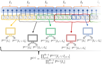
Figure 1: A $1D$ quantum system $\mathcal{S}$ is partitioned into adjacent intervals $I_{j}$ of size $k$, $|I_{j}|=k$. The purities over $I_{j}$ and $I_{j}\cup I_{j+1}$ are extracted using the classical-shadow approach Huang et al. (2020). Performing $M$ local measurements with respect to randomly chosen bases and classical post-processing operations, they yield faithful estimators for ${\rm Tr}[\rho_{I}^{2}]$, denoted by $\mathcal{P}^{(e)}[I]$. Such subsystem-purity estimators are then combined to obtain a prediction $\mathcal{P}^{(e)}$ for the global purity. The accuracy of the method is controlled by $k$ and the state correlation lengths.

In this work, we address precisely the problem of estimating global entropies and PT moments in many-qubit systems, and show that efficient strategies exist under the assumption that all spatial correlation lengths in the system are finite. This condition encompasses a large class of physically interesting cases, including ground and thermal states of local Hamiltonians, and is thus very natural when considering NISQ devices from the point of view of quantum simulation Georgescu et al. (2014); Tacchino et al. (2020); Daley et al. (2022).

In more detail, we focus on one-dimensional ($1D$) systems and put forward a strategy for the estimation of entropies and PT moments, requiring only polynomially-many measurements and post-processing operations. Our protocol is provably accurate for states satisfying a set of approximate factorization conditions (AFCs), which express the absence of long-range correlations and which are shown to be a general feature of short-range correlated states. The basic idea, which is conveyed in Fig. 1, is that the AFCs allow one to reconstruct global purities and PT moments from local information, which can be efficiently accessed by standard RM protocols Elben et al. (2023).

The proposed approach is different from tomographic methods relying on prior assumptions on the system state. There, a common strategy is to assume that the latter is described by a sufficiently simple ansatz wavefunction, and estimate the values of its free parameters. This logic was first put forward in the context of matrix-product states (MPSs) Perez-Garcia et al. (2007); Cirac et al. (2021); Cramer et al. (2010); Lanyon et al. (2017), while recently extended to matrix-product density operators (MPDOs) Qin et al. (2023); Baumgratz et al. (2013a, b); Holzäpfel et al. (2018); Lidiak et al. (2022), Gibbs states Kokail et al. (2021); Joshi et al. (2023); Anshu et al. (2021); Anshu and Arunachalam (2023); Rouzé and França (2021); Onorati et al. (2023), low-rank states Gross et al. (2010), stabilizers Montanaro (2017), and neural-network wavefunctions Kuzmin et al. (2023); Torlai et al. (2018); Zhao et al. (2023). While these methods may be practically very useful, they also face drawbacks. For instance, as we discuss in more detail in Sec. III.1, an accurate estimation of, say, global purities might require reconstructing the state up to exponential precision, thus leading to unpractical overheads in $N$. On the contrary, our approach does not learn the state wavefunction, targeting purities and PT moments directly, cf. Fig. 1.

Finally, we mention that our ideas could be extended, in some cases straightforwardly, to probe other types of quantities generally requiring exponentially many measurements, including participation entropies Luitz et al. (2014); Stéphan et al. (2009, 2010); Alcaraz and Rajabpour (2013); Stéphan (2014) or stabilizer Rényi entropies Leone et al. (2022), which were recently considered in the many-body setting Leone et al. (2022); Oliviero et al. (2022); Haug and Piroli (2023a, b); Lami and Collura (2023); Tarabunga et al. (2023); Niroula et al. (2023). In addition, while we will focus on $1D$ systems, where analytic and numerical analyses are simpler, we expect that our approach could be generalized to higher spatial dimensions. Therefore, our work also opens up a number of important directions for future research.

The rest of this manuscript is organized as follows. After reviewing a few preliminary notions and tools in Sec. II, we start by introducing the main ideas underlying our approach in Sec. III. To this end, we consider the class of so-called finite-depth quantum-circuit (FDQC) states, which provide an ideal toy model for short-range correlated many-body quantum states. Their minimal structure allows us to remove unnecessary technical complications from the discussion, and present the logic of our method in the simplest possible setting. We consider both purities (Sec. III.1) and PT moments (Sec. III.2), working out efficiency performance guarantees for their estimation.

The most general form of our protocol is presented in Sec. IV. After introducing the AFCs in Sec. IV.1, we rigorously derive performance guarantees for the accurate estimation of the purity and PT moments (Sec. IV.2) under the assumption that the state to be measured satisfies the AFCs. We then discuss the generality of the AFCs, proving that they are satisfied in translation-invariant MPDOs (Sec. IV.3), and presenting numerical evidence for their validity in thermal states of local Hamiltonian, cf. Sec. IV.4.

Next, in Sec. V we discuss a few natural examples of highly mixed states where bipartite entanglement can be detected for large system sizes by estimating just the first few PT moments. Since the latter can be very simply extracted by our approach, we argue that our results could be practically useful to probe mixed-state entanglement in experimentally available noisy quantum platforms. Finally, we report our conclusions in Sec. VI, while the most technical parts of our work are consigned to several appendices.

II Entanglement and randomized measurements

II.1 Mixed-state entanglement and PPT conditions

We consider a system of $N$ qubits, denoted by $\mathcal{S}$. Given a region $I\subset\mathcal{S}$, the associated Hilbert space is $\mathcal{H}_{I}\simeq\mathbb{C}^{\otimes 2|I|}$, where we denoted by $|I|$ the number of qubits in $I$. We will be interested in the Rényi entropies of the region $I$

$$S_{n}[I]=\frac{1}{1-n}{\ln\mathcal{P}_{n}[I]}\,,$$ (1)

where

$$\mathcal{P}_{n}[I]={\rm Tr}[\rho_{I}^{n}]\,,$$ (2)

and $\rho_{I}$ is the reduced density matrix on the region $I$. For $n=2$, $\mathcal{P}_{2}[I]$ coincides with the purity, which is a simple probe for the subsystem entropy, with $\mathcal{P}_{2}[I]=1$ and $\mathcal{P}_{2}[I]=2^{-|I|}$ for pure and maximally mixed states, respectively.

Consider now a partition of $\mathcal{S}$ into two disjoint sets $\mathcal{S}=A\cup B$, yielding $\mathcal{H}_{\mathcal{S}}=\mathcal{H}_{A}\otimes\mathcal{H}_{B}$. If the system is in a pure state $\ket{\psi}_{AB}\in\mathcal{H}_{\mathcal{S}}$, its bipartite entanglement is quantified by the Rényi entropies $S_{n}(\rho_{A})$ Nielsen and Chuang (2010). Conversely, when the state of the system is mixed, its entanglement can be quantified by the logarithmic negativity Vidal and Werner (2002); Plenio (2005)

$$\mathcal{E}(\rho)=\ln\sum_{j}|\lambda_{j}|\,,$$ (3)

where the sum is over all eigenvalues $\{\lambda_{j}\}_{j}$ of the operator $\rho_{AB}^{T_{A}}$, and $(\cdot)^{T_{A}}$ denotes partial transpose with respect to subsystem $A$. The spectrum of the PT density matrix, and hence the logarithmic negativity, is completely fixed by the PT moments

$$p_{n}={\rm Tr}\left[\left(\rho_{AB}^{T_{A}}\right)^{n}\right]\,,$$ (4)

for $n=1,2,...,{\rm dim}(\mathcal{H}_{A}\otimes\mathcal{H}_{B})$. Note that $p_{1}=1$, while the second PT moment coincides with the purity, $p_{2}=\mathcal{P}_{2}$ Elben et al. (2020a).

The importance of the PT moments is two-fold. On the one hand, they can be accessed directly via RMs Zhou et al. (2020); Elben et al. (2020a) (or using quantum interference Carteret (2005); Gray et al. (2018)), see Sec. II.2. On the other hand, the knowledge of the first few PT moments is enough to certify bipartite entanglement based on the non-positivity of the partial-transposed density matrix Carteret (2016); Elben et al. (2020a); Neven et al. (2021); Zhou et al. (2020); Yu et al. (2021b), or to detect different types of entanglement structures Carrasco et al. (2022). In this work, we will consider a particular set of conditions on the PT moments to certify bipartite entanglement, which were derived in Refs. Elben et al. (2020a); Yu et al. (2021b) and which we call the $p_{n}$-PPT conditions. Denoting by SEP the set of separable, i.e. not entangled, states in $\mathcal{S}$, the $p_{n}$-PPT conditions take the form

$$\rho\in{\rm SEP}\Rightarrow p_{n}p_{n-2}\geq p_{n-1}^{2}\,.$$ (5)

Therefore, when the state of the system $\rho$ violates the $p_{n}$-PPT conditions, it is entangled, and the difference $p_{n-1}^{2}-p_{n}p_{n-2}$ is a probe for mixed-state entanglement. Note that, for $n=3$, Eq. (5) coincides with the relation first derived in Ref. Elben et al. (2020a). These conditions are in general not optimal and are a strict subset of those derived in Ref. Yu et al. (2021b); Neven et al. (2021). Still, their simplicity makes them particularly convenient for our purposes.

II.2 Randomized measurements and classical shadows

In this section, we recall the basic aspects of RMs used in our work. While the logic explained in the next sections may be implemented in different ways, we will focus on a set of protocols making use the (local) classical shadows introduced in Ref. Huang et al. (2020), a prominent element in the RM toolbox Elben et al. (2023). We briefly recall the main aspects of the formalism, while we refer to Refs. Huang et al. (2020); Elben et al. (2023) for a thorough introduction.

In what follows, we denote by $\ket{0}_{j}$ and $\ket{1}_{j}$ the basis elements of the local computational basis corresponding to qubit $j$, spanning $\mathcal{H}_{j}\simeq\mathbb{C}^{2}$. In the classical-shadow framework, one performs a set of $M$ measurements (one per experimental run, each labeled by an integer $r$), consisting of local unitary operations $\prod_{j}u_{j}^{(r)}$ followed by a projective measurement onto the computational basis

$$|k_{1},\ldots k_{N}\rangle=\otimes_{j=1}^{N}\ket{k_{j}}_{j}\,,$$ (6)

with $k_{j}=0,1$. The unitaries are sampled from a Haar-random ensemble, identically and independently for each qubit $j$ and experimental run $r$, see Fig. 2. Denoting by $\{k^{(r)}_{j}\}$ the set of outcomes of this two-step process, the values $\{k^{(r)}_{j}\}$ and the unitaries $\{u_{j}^{(r)}\}$ are used to define the so-called classical shadows

$$\rho^{(r)}_{\mathcal{S}}=\bigotimes_{i\in\mathcal{S}}\left[3\left(u_{i}^{(r)}\right)^{\dagger}\ket{k_{i}^{(r)}}\bra{k_{i}^{(r)}}u_{i}^{(r)}-\openone_{2}\right]\,,$$ (7)

which can be classically stored in an efficient way.

As mentioned, the measurement protocol does not depend on the observable of interest. Rather, one adapts the post-processing operations on the classical shadows based on the quantity to be estimated. For instance, given any observable $O$, an estimator for its expectation value is

$$\hat{o}=\frac{1}{M}\sum_{r=1}^{M}{\rm Tr}[O\rho_{\mathcal{S}}^{(r)}]\,.$$ (8)

It is easy to see that $\hat{o}$ is faithful, i.e. unbiased, while different bounds for the statistical variance of this estimator may be derived depending on the locality properties of $O$ Huang et al. (2020); Elben et al. (2023).

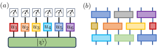
Figure 2: $(a)$: Within the classical-shadow approach, each measurement process consists of random on-site unitaries followed by local projective measurements. Their outcomes are stored and later post-processed to construct the classical shadows. $(b)$: Pictorial representation of a local finite-depth quantum circuit. The gates are arranged in a brickwork pattern, forming layers of mutually commuting unitary operations acting on pairs of neighboring qubits. Lower (upper) dangling legs correspond to the input (output) qubits. The depth of the circuit is the number of applied layers. In this picture, the depth is $\ell=3$.

It is important to recall that classical shadows also give access to entropy and PT moments. Let us consider in particular the purity, which is given by Eq. (2) for $n=2$. For this quantity, the classical shadows allow us to write the estimator Huang et al. (2020)

$$\mathcal{P}_{2}^{(e)}[I]=\frac{1}{M(M-1)}\sum_{r\neq r^{\prime}}{\rm Tr}\left(\rho_{I}^{(r)}\rho_{I}^{\left(r^{\prime}\right)}\right)\,,$$ (9)

where $\rho_{I}$ is defined as in Eq. (7). $\mathcal{P}^{(e)}[I]$ is a faithful estimator. Note that, alternatively, one can use another estimator for the purity Elben et al. (2018); Brydges et al. (2019); Elben et al. (2019) that provides robustness against miscalibration errors using the same data. The statistical errors associated with $\mathcal{P}_{2}^{(e)}[I]$ are quantified by its variance, which can be bounded by Huang et al. (2020); Elben et al. (2020a); Rath et al. (2021a)

$${\rm Var}\left[\mathcal{P}_{2}^{(e)}[I]\right] \leq 4\left(\frac{2^{|I|}\mathcal{P}_{2}[I]}{M}\right)+2\left(\frac{2^{2|I|}}{M-1}\right)^{2}\,,$$ (10)

where $|I|$ denotes the number of qubits in $I$. This bound is known to be essentially optimal Elben et al. (2020a); Rath et al. (2021a), telling us that an exponentially large number of measurements is needed to estimate the purity.

The PT moments (4) can be treated similarly. In this case, one constructs the estimator Elben et al. (2020a)

$$p^{(e)}_{n}[AB] =\frac{1}{n!}\binom{M}{n}^{-1}$$

$$\times\sum_{r_{1}\neq r_{2}\neq\ldots\neq r_{n}}\operatorname{Tr}\left[[\rho_{AB}^{\left(r_{1}\right)}]^{T_{A}}\cdots[\rho_{AB}^{\left(r_{n}\right)}]^{T_{A}}\right]\,.$$ (11)

Once again, $p^{(e)}_{n}[AB]$ is faithful and it is possible to derive explicit bounds on its variance, although it becomes increasingly involved for higher $n$. For instance, for $n=3$ one has Elben et al. (2020a); Rath et al. (2021a)

$$\operatorname{Var}\left[p^{(e)}_{3}[AB]\right] \leq 9\frac{2^{|AB|}}{M}\operatorname{Tr}\left(\rho_{AB}^{4}\right)$$

$$+ 18\frac{2^{3|AB|}}{(M-1)^{2}}p_{2}[AB]+6\frac{2^{6|AB|}}{(M-2)^{3}}\,.$$ (12)

Estimating the statistical errors by the variance, Eqs. (10) and (II.2) imply that, in order to guarantee an accurate reconstruction of the purity and PT moments of the system, exponentially-many measurements in its size are needed. As mentioned, this makes it unfeasible to significantly scale up previous experiments making use of this strategy Brydges et al. (2019); van Enk and Beenakker (2012); Elben et al. (2018, 2019); Huang et al. (2020); Elben et al. (2020a). The goal of this work is to show that these limitations may be overcome under assumptions which are very common in the context of many-body physics, and thus also natural from the point of view of quantum simulation. Namely, we will put forward a set of protocols for entropy and entanglement estimation which are provably efficient assuming that all spatial correlation lengths of the state to be measured are finite. We will focus on $1D$ systems, where analytic and numerical analyses are simpler, although we expect that our approach could be generalized to higher spatial dimensions, see Sec. VI.

III A toy model for the estimation protocol

In this section we introduce the main ideas underlying our approach, focusing on a simplified setting where we can get rid of unnecessary technical complications. We analyze the case of FDQC states, where the state to be measured is prepared by a shallow (local) quantum circuit

$$\rho=U^{(\ell)}\left(\bigotimes_{j=1}^{L}\sigma_{j}\right)\left[U^{(\ell)}\right]^{\dagger}\,,$$ (13)

where $L$ is length of the system, i.e. the number of qubits (we use the letter $L$ instead of $N$, as in the previous section, to emphasize that we are focusing on the $1D$ case). Here $\sigma_{j}$ are arbitrary single-qubit density matrices, while $U^{(\ell)}$ is a local circuit of depth $\ell$, namely $U^{(\ell)}=V_{\ell}\cdots V_{2}V_{1}$, where $V_{j}$ contains quantum gates acting on disjoint pairs of nearest-neighbor qubits, cf. Fig. 2. We will assume that $\ell$ is fixed, i.e. not increasing with the system size. We do not ask for translation symmetry and, unless specified otherwise, assume open boundary conditions. The gates making up $U^{(\ell)}$ can be arbitrary, i.e. they need not be taken out of some finite gate set. The FDQC states (13) have a very simple structure from the point of view of many-body physics, but are known to approximate physically-interesting states such as MPSs Piroli et al. (2021); Malz et al. (2023) and, more generally, ground states of gapped local Hamiltonians Chen et al. (2010); Hastings (2013); Zeng et al. (2015); Zeng and Wen (2015) .

Throughout this section, we will assume that we know that the state of the system is exactly of the form (13) for some finite $\ell$. We develop a protocol to efficiently estimate the purity and the PT moments of such a state, based on this knowledge. The protocol only takes the depth of the circuit, $\ell$, as an input and does not make use of state tomography. In fact, it will be later generalized replacing the assumption of the FDQC structure with the AFCs, which make no explicit reference to the form of the state wavefunction.

III.1 Purity estimation: Factorization formula

The starting point of our method is a factorization property for powers of the system density matrix. Let $I$ be any interval of adjacent qubits ($I$ can coincide with the full system $\mathcal{S}$). Consider a partition $I=A\cup B\cup C$, where $B$ separates $A$ and $C$ and denote by $|B|$ the number of qubits in $B$, cf. Fig. 3$(a)$. Based on the fact that state is prepared by a finite depth circuit, Eq. (13), one can prove

$${\rm Tr}(\rho_{I}^{2})=\frac{{\rm Tr}_{AB}(\rho_{AB}^{2}){\rm Tr}_{BC}(\rho_{BC}^{2})}{{\rm Tr}_{B}(\rho_{B}^{2})}\,,$$ (14)

for any partition with $|B|\geq 2\ell-1$, where $\rho_{X}$ denotes the density matrix reduced to the interval $X$ and $XY$ is a short-hand notation for $X\cup Y$. Now, let $\{I_{j}\}_{j=1}^{R}$ be a collection of adjacent intervals covering the system $\mathcal{S}$, with $|I_{j}|=k\geq 2\ell-1$, and assume without loss of generality that $R=L/k$ is an integer, cf. Fig. 1. By applying Eq. (14) iteratively, we arrive at

$${\rm Tr}(\rho^{2})=\frac{\prod_{j=1}^{R-1}{\rm Tr}_{I_{j}\cup I_{j+1}}(\rho^{2}_{I_{j}\cup I_{j+1}})}{\prod_{j=2}^{R-1}{\rm Tr}_{I_{j}}\left[\rho_{I_{j}}^{2}\right]}\,,$$ (15)

where $\rho$ is the system density matrix (13). A proof of Eqs. (14) and (15) is given in Appendix A.

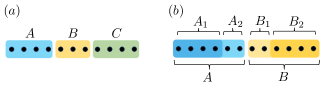
Figure 3: $(a)$: Partition considered in Eq. (14): A $1D$ interval $I$ is divided into three disjoint regions $A$, $B$, and $C$, where $B$ separates $A$ and $C$. $(b)$: Partition considered in Eq. (25): A $1D$ interval $I$ is divided into two halves, $A$ and $B$. Each half is partitioned into two regions $A=A_{1}\cup A_{2}$, $B=B_{1}\cup B_{2}$

Equation (15) is remarkable because its right hand side (RHS) only depends on the purities of subsystems containing up to $2k$ qubits, and thus gives us a natural basis for an efficient estimation strategy of the global purity. The idea is to first reconstruct the “local” purities ${\rm Tr}[\rho_{I}^{2}]$ (with either $I=I_{j}$ or $I=I_{j}\cup I_{j+1}$), and subsequently plug their estimated values in the RHS of Eq. (15), yielding the global purity estimate. This method is more efficient than directly targeting ${\rm Tr}(\rho^{2})$, as the local purities can be reconstructed from a number of measurements growing exponentially in $k$, not in $L$, see Eq. (10). Below, we give a more precise description of the protocol, proving that an accurate estimation of the purity only requires a polynomial (in $L$) number of measurements and post-processing operations.

We consider performing $M_{I}$ measurements (i.e. experimental runs) to estimate the purity of each interval $I$, with $I=I_{j}$ or $I=I_{j}\cup I_{j+1}$, see Eq. (15). The set of measurements $M_{I}$ is only used to determine the purity over $I$ and for simplicity we perform the same number of measurement $M_{I}=M$ for each interval. Although this increases the total number of experiments $M_{T}$ by a factor $L$, since

$$M_{T}=\sum_{I}M_{I}\propto LM\,,$$ (16)

this procedure guarantees that statistical errors associated with distinct regions are independent and facilitate their rigorous analysis. For each interval, we then construct the estimators $\mathcal{P}^{(e)}[I]$ given in Eq. (9), and define

$$r^{(e)}_{2}=\frac{\prod_{j=1}^{R-1}\mathcal{P}_{2}^{(e)}[{I_{j}\cup I_{j+1}}]}{\prod_{j=2}^{R-1}\mathcal{P}_{2}^{(e)}[I_{j}]}\,,$$ (17)

which is our estimator for the global purity. Since the latter is typically exponentially small in $L$, we quantify the accuracy of $r^{(e)}_{2}$ by the relative error

$$\varepsilon_{r}=\left|\frac{r_{2}^{(e)}}{\mathcal{P}_{2}}-1\right|\,.$$ (18)

Next, we seek to bound the number of measurements required to guarantee that $\varepsilon_{r}$ is small with high probability. This problem is solved in Appendix B.1, where we prove the following result: for any arbitrarily small $\delta>0$, choosing

$$M\geq{\rm max}\left\{2^{8k},L^{2}\frac{2^{4k+10}}{k^{2}\delta^{2}}\right\}\,,$$ (19)

the probability that $|\varepsilon_{r}|\geq\delta$ satisfies

$${\rm Pr}\left[|\varepsilon_{r}|\geq\delta\right]\leq\frac{2^{4k+11}L^{3}}{\delta^{2}k^{3}M}\,,$$ (20)

where we recall that $k=|I_{j}|$. The proof of Eq. (20) is based on a careful analysis of how the error on each factor in (17) affects the global purity, making use of the statistical independence of $\mathcal{P}^{(e)}_{2}[I]$ for different $I$ and the so-called Chebyshev’s inequality. Eqs. (16), (19), and  (20) then imply that polynomially-many (in $L$) measurements and post-processing operations are enough to accurately estimate the purity, as anticipated.

Before concluding this section, a few remarks are in order. First, it is important to note that the individual factors in the formula (17) could also be extracted using different RM schemes or even standard tomography for the density matrices $\rho_{I}$. Indeed, the possibility of estimating the global purity from polynomially-many measurements does not depend on the fact that we are using classical shadows, but rather on the factorization property (17) (since its RHS only involves local subsystems). Still, classical shadows and RMs in general offer several advantages compared to state tomography. For instance, while RM schemes to estimate ${\rm Tr}[\rho_{I}^{2}]$ require a number of measurements scaling exponentially in $|I|$, the exponents are typically favorable compared to tomography Brydges et al. (2019); Rath et al. (2023); Stricker et al. (2022). In addition, classical shadows make it very easy to rigorously bound statistical errors, facilitating the analyses presented throughout this work.

Second, taking the logarithm of Eq. (15), we obtain

$$S^{(2)}(\rho)=\sum_{j=1}^{R-1}S^{(2)}(\rho_{I_{j}\cup I_{j+1}})-\sum_{j=2}^{R-1}S^{(2)}(\rho_{I_{j}})\,,$$ (21)

where $S^{(2)}(\rho)=-\ln{\rm Tr}\rho^{2}$ is the second Rényi entropy. Therefore, our results can equivalently be formulated in terms of Rényi entropies, rather than purities (note that a small relative error on the latter implies a small additive error on the Rényi entropy).

Finally, as the state (13) can be represented exactly as a matrix-product operator (MPO) Silvi et al. (2019), it is instructive to compare our strategy with those based on MPDO tomography  Qin et al. (2023); Baumgratz et al. (2013a, b, b); Holzäpfel et al. (2018); Lidiak et al. (2022). In many cases, these methods can efficiently provide an estimate of the system density matrix $\rho^{(e)}$, satisfying

$$||\rho^{(e)}-\rho||_{1}\leq\delta\,,$$ (22)

where $||\cdot||_{1}$ denotes the trace norm, while $\delta=O(L^{-\alpha})$ is a small parameter vanishing polynomially in $L$. While this approximation allows us to accurately estimate the expectation value of any local observable, it might not be enough to extract the global Rényi-$2$ entropy. Indeed, given $\rho$ and $\sigma$ with $\delta=||\rho-\sigma||_{1}$, we have the following bound, which is known to be tight in general Audenaert (2007); Chen et al. (2017)

$$|S^{(2)}(\rho)\!-\!S^{(2)}(\sigma)| \leq 2^{L}\left[1\!-\!(1\!-\!2\delta)^{2}\right.\!-\!\left.\frac{4\delta^{2}}{\left(2^{L}\!-\!1\right)}\right]$$

$$\sim 2^{L}\delta\,.$$ (23)

Therefore, a precise estimation of the Rényi-$2$ entropy requires an exponentially accurate reconstruction of the system density matrix, typically leading to unpractical overheads in $L$ . Instead, our method gets around this technical issue, as it does not rely on state tomography.

III.2 The normalized PT-moment estimation

The ideas presented in the previous section may be applied to the PT moments, although a few subtleties must be taken into account. Denoting by $p^{(e)}_{n}$ our estimate for $p_{n}$, one is tempted to ask for a protocol that makes the relative error $|p^{(e)}_{n}/p_{n}-1|$ sufficiently small. This is, however, problematic: contrary to the moments $\mathcal{P}_{n}$, it is non-trivial to bound $|p_{n}|$ from below by a positive number. In order to get around this issue, we define the normalized PT moment

$$\tilde{p}_{n}[AB]=\frac{p_{n}[AB]}{\mathcal{P}_{n}[A]\mathcal{P}_{n}[B]}\,,$$ (24)

and, instead of focusing on the relative error, we ask for an accurate estimate of $\tilde{p}_{n}$ up to a small additive error. The motivation for this choice is two-fold. First, as it will be clear later, for FDQC states one can show that $\tilde{p}_{n}[AB]$ is independent of the system size. Therefore, contrary to the purity, one does not have to deal with numbers which are exponentially small in $L$. Second, we will see in Sec. V that entanglement certification based on the $p_{n}$-PPT conditions requires approximating $\tilde{p}_{n}[AB]$ up to a small additive error.

In order to estimate the normalized PT moment (24), we once again rely on certain factorization properties of the density matrix. Consider the FDQC state (13) and take a partition of the system as in Fig. 3$(b)$, with $|B_{1}|=|A_{2}|=k\geq 2\ell-1$, where $\ell$ is the depth of the circuit. As we show in Appendix A.2, one can prove

$$\!{\rm Tr}\left[\!\left(\rho_{AB}^{T_{A}}\right)^{n}\right]\!=\!{\rm Tr}\left[\!\left(\rho_{A_{2}B_{1}}^{T_{A_{2}}}\right)^{n}\right]\!\frac{{\rm Tr}_{A}[\rho_{A}^{n}]{\rm Tr}_{B}[\rho_{B}^{n}]}{{\rm Tr}_{A_{2}}[\rho_{A_{2}}^{n}]{\rm Tr}_{B_{1}}[\rho_{B_{1}}^{n}]}.$$ (25)

This equation implies

$$\tilde{p}_{n}[AB]=s_{n}[A_{2}B_{1}]\,,$$ (26)

where we defined

$$s_{n}[XY]=\frac{{\rm Tr}\left[\left(\rho_{XY}^{T_{X}}\right)^{n}\right]}{{\rm Tr}_{X}[\rho_{X}^{n}]{\rm Tr}_{Y}[\rho_{Y}^{n}]}\,.$$ (27)

Note that $s_{n}[A_{2}B_{1}]$ only depends on the density matrix of a local subsystem and does not scale with the system size, as anticipated. Therefore, it is possible to obtain an accurate estimate from a number of measurements and post-processing operations independent of $L$, for any arbitrary small additive error.

To see this explicitly, we consider the following protocol. We introduce an estimator for $s_{n}[A_{2}B_{1}]$, namely

$$s^{(e)}_{n}=\frac{p^{(e)}_{n}[A_{2}B_{1}]}{\mathcal{P}^{(e)}_{n}[A_{2}]\mathcal{P}^{(e)}_{n}[B_{1}]}\,.$$ (28)

The estimators for the moments $\mathcal{P}^{(e)}_{n}[A_{2}]$, $\mathcal{P}^{(e)}_{n}[B_{1}]$ and the PT-moment $p^{(e)}_{n}[A_{2}B_{1}]$ are defined in Eq. (II.2). We compute each of them out of $M$ different classical shadows, so that the total number of experimental runs is $M_{T}=3M$. This is done so that the statistical errors are independent, facilitating their analysis. After these steps, we obtain an estimate for $s_{n}[A_{2}B_{1}]$, and thus, due to Eq. (25), for $\tilde{p}_{n}[AB]$.

Importantly, we can bound the additive statistical error which affects our estimate, namely

$$\varepsilon_{a}=\left|s_{n}^{(e)}-\tilde{p}_{n}[AB]\right|\,.$$ (29)

For instance, focusing for simplicity on the case $n=3$, we prove in Appendix B.2 the following result: for any small $\delta>0$ and choosing

$$M\geq 27\frac{2^{11k+9}}{\delta^{2}}\,,$$ (30)

we have

$${\rm Pr}\left[\left|s^{(e)}_{3}-\tilde{p}_{3}[AB]\right|\geq\delta\right]\leq 81\frac{2^{11k+9}}{M\delta^{2}}\,,$$ (31)

where $|A_{2}|=|B_{1}|=k\geq 2\ell-1$, with $\ell$ being the circuit depth. This result is proved by the same techniques used to derive Eq. (20).

Equation (31) states that a number of measurements not scaling with the system size is enough to guarantee that $\tilde{p}_{3}$ is approximated with arbitrary precision and high probability. Explicit performance guarantees such as (31) for higher integer values of $n$ are more cumbersome to derive, and will be omitted. Still, based on the analysis presented in Appendix B.2, one can easily see that inequalities of the form (31) hold for higher $n$ too, where the RHS is always independent of $L$.

IV Finite-range correlated states

In this section we present and discuss the most general form of our protocols. First, in Sec. IV.1 we give the definition of the AFCs, which state that the $n$-th powers of the system density matrix effectively factorize over regions of size smaller than some length scales $\xi_{n}$. Our definition might appear arbitrary at first, but we show later that such AFCs hold in large classes of states (see Secs. IV.3 and  IV.4). Next, in Sec. IV.2 we describe a protocol for purity and PT moment estimation in states satisfying the AFCs. Such protocols take as an input the value of the length scales $\xi_{n}$ (assumed to be known) and the desired accuracy, yielding as an output the numerical estimations for the purity and PT moments. The protocols only require polynomially-many (in $L$) measurements and post-processing operations. In addition, we can rigorously prove that the estimation errors are smaller than the desired threshold with high probability. Finally, we discuss the generality of the AFCs, proving analytically that they hold for MPDOs (Sec. IV.3) and presenting numerical evidence for their validity in Gibbs states of local Hamiltonians (Sec. IV.4).

IV.1 The approximate factorization conditions

The strategies developed so far rely on exact factorization conditions on the system density matrix, which are related to the sharp light-cone structure of correlation functions in FDQC states Farrelly (2020); Piroli and Cirac (2020); Piroli et al. (2021). Away from these ideal cases, Eqs. (14) and (25) do not hold, but it is natural to conjecture that they can be modified taking into account exponential corrections over scales governed by the system correlation lengths. This is done in this section, where we introduce a set of AFCs generalizing Eqs. (14) and (25), respectively.

Given a state $\rho$, we say that it satisfies the purity AFC if there exist $\alpha_{2},\beta_{2},k_{c}>0$ such that, for any interval $I=A\cup B\cup C$ as in Fig. 3$(a)$, with $|B|=k\geq k_{c}$, we have

$$\!\!\!\left|{\rm Tr}(\rho_{I}^{2})^{-1}\frac{{\rm Tr}_{AB}(\rho_{AB}^{2}){\rm Tr}_{BC}(\rho_{BC}^{2})}{{\rm Tr}_{B}(\rho_{B}^{2})}\!-1\right|\leq\alpha_{2}e^{-\beta_{2}|B|}.$$ (32)

Similarly, we say that $\rho$ satisfies the PT-moment AFCs if there exist $\alpha_{n},\beta_{n}>0$ and an integer $k_{c}$ such that

$$\left|\tilde{p}_{n}[AB]-s_{n}[A_{2}B_{1}]\right|\leq\alpha_{n}e^{-\beta_{n}(|A_{2}|+|B_{1}|)}\,,$$ (33)

for all partitions as in Fig. 3$(b)$ with $|B_{1}|=|A_{2}|=k\geq k_{c}$. Here $\tilde{p}_{n}[AB]$ and $s_{n}[A_{2}B_{1}]$ are defined in Eqs. (24) and  (27), respectively. Equations (32) and (33) obviously generalize (14) and (25), introducing exponential corrections over length scales $\xi_{n}=\beta^{-1}_{n}$.

While the definitions (32) and (33) might appear arbitrary at first, we show later that such AFCs hold in large classes of states (see Secs. IV.3 and  IV.4). In the next section, we assume that the AFCs hold, and describe a protocol for purity and PT moment estimation. We stress that we do not need any additional assumption on the state to be measured. For instance, we do not require that it can be represented efficiently by an MPDO, making our approach very general.

Our protocols take as an input the values of $\alpha_{n}$, $\beta_{n}$, and the desired accuracy. For instance, the purity estimation protocol takes as an input $\alpha_{2}$, the correlation length $\xi_{2}=\beta^{-1}_{2}$, and the target threshold relative error $\delta$. Importantly, it is not necessary to know the values of $\alpha_{2}$ and $\beta_{2}$ exactly: it is sufficient to have two estimates $\tilde{\alpha}_{2}$, $\tilde{\xi}_{2}$, which upper-bound them. This is because if $\alpha_{2}\leq\tilde{\alpha}_{2}$ and $\xi_{2}\leq\tilde{\xi}_{2}$, then Eq. (32) also holds replacing $\alpha_{2}$ and $\beta_{2}$ with $\tilde{\alpha}_{2}$ and $\tilde{\beta}_{2}=\tilde{\xi}_{2}^{-1}$, respectively. We can choose $\tilde{\alpha}_{2}$ and $\tilde{\xi}_{2}$ arbitrarily, but the number of measurements and post-processing operations increase parametrically with $\tilde{\alpha}_{2}$ and $\tilde{\xi}_{2}$, see Eq. (35). Therefore, the more accurately we can estimate the values of $\alpha_{2}$ and $\beta_{2}$, i.e. the more information we have on the state to be measured, the more efficiently we can estimate the purity and, similarly, the PT moments.

Finally, suppose that, for given state $\rho$, we have an ansatz for $\alpha_{2}$ and $\xi_{2}$. From the experimental point of view, an important question is whether it is possible to efficiently certify that Eq. (32) holds, with the ansatz values $\alpha_{2}$ and $\xi_{2}$, for the state to be measured. While at the moment this is an open question, a simple consistency check consists in repeating the purity estimation protocol (explained in IV.2) for increasing values of the input ansatz values $\alpha_{2}$ and $\xi_{2}$, and checking that the estimated value for the purity does not change, up to the expected precision. If the estimated purity does change, this is a “red flag” signalling the failure of the AFCs. We refer to Sec. VI for further discussions on the possibility to efficiently certify the validity of the AFCs.

IV.2 Estimation protocols for states satisfying the AFCs

First, we consider estimating the global purity of a state satisfying the AFCs (32). We assume the following:

• we know that the system is prepared in a state $\rho$ satisfying the AFCs (32);

• we know two numerical values $\alpha_{2}$ and $\beta_{2}$ for which Eq. (32) is satisfied.

Below, we detail our protocol to efficiently estimate the purity. The proof that the protocol works is non-trivial and is presented in detail in Appendix C. Intuitively, we use the fact that, because of the AFC (32), the estimator $r^{(e)}_{2}$ defined in Eq. (17) yields a good approximation for the purity, for values of $|I_{j}|$ which grow mildly (logarithmically) in $L$.

The protocol takes as an input the values of $\alpha_{2}$ and $\beta_{2}$, and consists of the following steps:

1. Choose the desired relative error $\delta$ on the purity. This can be any arbitrarily small number $\delta>0$;

2. Take a partition of the system as in Fig. 1, where $|I_{j}|=k$ and choose

   $$k\geq\xi_{2}\ln(7\alpha_{2}L/\delta)\,,$$ (34)

   where $\xi_{2}=\beta_{2}^{-1}$. The reason for the functional form appearing in the RHS is technical and explained in Appendix C;

3. As in Sec. III.1, perform $M_{I}=M$ classical-shadow measurements to estimate the purity of each interval $I$, with $I=I_{j}$ or $I=I_{j}\cup I_{j+1}$ [we use the set of measurements $M_{I}$ to only determine the purity over $I$, so that the total number of experimental runs is given by (16)].

4. From the classical shadows obtained out of the measurements, compute $r^{(e)}_{2}$ defined Eq. (17). This is the output of our protocol, giving us an estimate for the global purity.

As mentioned, it is intuitive that the output of this protocol $r^{(e)}_{2}$ is, with high probability, an accurate approximation for the purity. This is proven rigorously in Appendix C, where we show

$$\!\!{\rm Pr}\left[\left|(r_{2}^{(e)}/\mathcal{P}_{2})-1\right|\geq\delta\right]\!\leq\frac{7^{2}2^{11}L^{3}}{\delta^{2}M}\left(\frac{7\alpha_{2}L}{\delta}\right)^{4\xi_{2}\ln 2}\,.$$ (35)

Therefore, by a polynomial number of measurements $M$ we can guarantee that the probability that the relative error $|r_{2}^{(e)}/\mathcal{P}_{2}-1|$ is larger than $\delta$ is arbitrarily small. This formalizes the anticipated result.

Note that $r^{(e)}_{2}$ defined above is a faithful estimator for the quantity

$$r_{2}=\frac{\prod_{j=1}^{R-1}{\rm Tr}_{I_{j}\cup I_{j+1}}(\rho^{2}_{I_{j}\cup I_{j+1}})}{\prod_{j=2}^{R-1}{\rm Tr}_{I_{j}}\left[\rho_{I_{j}}^{2}\right]}\,,$$ (36)

but because (15) does not hold exactly, it is not a faithful estimator of the global purity $\mathcal{P}_{2}$. Still, it is a good approximation, as it is clear from the relation

$$\left|\frac{r_{2}}{\mathcal{P}_{2}}-1\right|\leq\frac{4\alpha_{2}L}{k}e^{-\beta_{2}k}\,,$$ (37)

which holds for

$$k\geq\xi_{2}\ln(2\alpha_{2}L)\,,$$ (38)

and follows directly from (32), cf. Appendix C. In practice, the RHS of (37) makes it necessary to consider intervals $I_{j}$ whose length $k$ grows logarithmically in $L$ to keep the error below the desired threshold.

A similar protocol works for the PT moments. In this case, a number of measurements which does not scale with the system size is enough to guarantee arbitrary accuracy with high probability, cf. Appendix C. We note that the results of this section imply that the number of post-processing operations to estimate the purity and PT moments is also at most polynomial in $L$. This is because the estimators (9) and (II.2) are constructed summing a number of terms which is polynomial in $M$, and hence at most polynomial in $L$.

In the rest of this section, we discuss the generality of the AFCs. We prove analytically that they hold for the important class of translation-invariant MPDOs and provide numerical evidence that they are also satisfied by thermal states of local Hamiltonians. These results showcase the generality and versatility of our approach.

IV.3 Proof of AFCs in Matrix Product Density Operators

We now focus on MPDOs, a very general class of states providing accurate approximations for several short-range correlated density matrices, including thermal states of local Hamiltonians Cirac et al. (2017, 2021). We study the translation-invariant case, where we can provide analytic results. We recall that a translation-invariant MPDO $\sigma$ is defined by a four-index tensor $A^{j,k}_{a,b}$, with $j,k=0,1$ and $a,b=0,1\ldots\chi-1$, where $\chi$ is its bond dimension Silvi et al. (2019). For a system size $L$, its matrix elements read

$$\braket{i_{1},\ldots,i_{L}}{\sigma_{L}}{j_{1},\ldots,j_{L}}\!=\!A^{i_{1},j_{1}}_{a_{1},a_{2}}A^{i_{2},j_{2}}_{a_{2},a_{3}}\cdots A^{i_{L},j_{L}}_{a_{L},a_{1}},$$ (39)

where repeated indices are summed over. This defines a family of normalized states

$$\rho_{L}=\frac{\sigma_{L}}{{\rm Tr[\sigma_{L}]}}\,.$$ (40)

Using the standard notation from tensor-network theory Silvi et al. (2019), we can represent Eq. (39) as

$$\sigma_{L}=\raisebox{-11.0pt}{\includegraphics[scale={0.21}]{MPDO.pdf}}$$ (41)

Here each circle correspond to a tensor $A^{j,k}_{a,b}$. Lower and upper legs are associated with input and output degrees of freedom, respectively, while the remaining ones correspond to the “virtual” indices $a_{j}=0,\ldots\chi-1$. Note that contracted legs indicate pairs of indices which are summed over.

We first focus on the purity. We are able to show that MPDOs satisfy the purity AFCs under a few technical assumptions, which encode the fact that all correlation lengths are finite but are otherwise very general. Technically, we impose a few conditions on the spectrum and eigenstates of the transfer matrices

$$\tau_{n}=\raisebox{-45.0pt}{\includegraphics[scale={0.44}]{transfer.pdf}}\,,$$ (42)

where the top and bottom legs are contracted. Informally, we ask that $\tau_{1}$ and $\tau_{2}$ have non-degenerate eigenvalues with largest absolute value, and that the corresponding eigenstates are not orthogonal. These conditions are general in the sense that one needs to choose fine-tuned examples to violate them. We refer the reader to Appendix D for a precise statement and a detailed discussion.

Under these assumptions, we show that $\rho_{L}$ satisfies the purity AFCs. Note that, different from the rest of this work, here we are considering periodic boundary conditions. Since Eq. (32) was introduced for open boundary conditions, we consider directly its global version (37), which can immediately be generalized to the periodic case. Clearly, the expression for $r_{2}$ must be modified with respect to (36): taking into account periodic boundary conditions, we replace it with

$$r_{2}=\frac{\prod_{j=1}^{R}{\rm Tr}_{I_{j}\cup I_{j+1}}(\sigma^{2}_{I_{j}\cup I_{j+1}})}{\prod_{j=1}^{R}{\rm Tr}_{I_{j}}\left[\sigma_{I_{j}}^{2}\right]}\,,$$ (43)

where we assume without loss of generality that $R=L/k$ is an integer, while the normalization factors ${\rm Tr}[\sigma^{2}]$ cancel out.

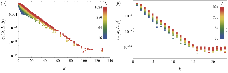
Figure 4: Relative error $\varepsilon_{r}(k,L,\beta)$, defined in Eq. (49), as a function of $k$, for $\beta=2$ and different values of $L$. In the left and right plots we report numerical data corresponding to the Ising and XXZ spin chains, respectively. In the former case, we chose $h_{x}=1.1$, $h_{z}=-0.04$, while the maximal bond dimension used in the computation is $\chi=32$. In the latter case, we set $\Delta=2$, while $\chi=64$.

The task of proving Eq. (37) [using the definition (43)] is carried out in Appendix D. There, we derive the following statement: given the family of MPDOs $\rho_{L}$ as above, there exist $\zeta>0$, and $C>0$ (independent of $L$) such that, for any integer $k\geq k_{\rm min}$, with

$$k_{\rm min}={\rm max}\left\{1,\zeta\ln(20C\chi^{2}L)\right\}\,,$$ (44)

we have

$$\left|\frac{r_{2}}{\mathcal{P}_{2}}-1\right|\leq\chi^{2}(80C+32)\frac{L}{k}e^{-k/\zeta}\,,$$ (45)

for all $L\geq{\rm max}\{\zeta\ln(2^{5}\chi^{2}),4k+\zeta\ln(2\chi)\}$. The correlation length $\zeta$ and the constant $C$ depend on both the eigenvalues and eigenvectors of the transfer matrices $\tau_{1}$ and $\tau_{2}$, cf. Appendix D. Therefore, the purity approximate factorization formula (37) holds with $\alpha_{2}=\chi^{2}(20C+8)$, and $\beta_{2}=1/\zeta$. In turn, using the results of the previous sections, this implies that the purity of MPDOs can be estimated efficiently using our approach.

Similarly, the AFCs for PT moments could be verified analytically for bulk-translation-invariant MPDOs with suitable open boundary conditions. This is slightly more involved, as a few additional technical assumptions on the boundaries are needed. For this reason, we do not discuss this explicitly. Instead, the AFCs for PT moments will be numerically analyzed in detail in the next section, together with the purity AFCs, for the physically interesting case of Gibbs states of local Hamiltonians in a few concrete examples.

IV.4 Numerical study of AFCs in Gibbs states

Figure 5: Numerical results for the minimal region size $k^{\ast}(\delta,L)$ required to achieve a specified precision $\delta$ of purity estimation, see Eq. (50). In the plots we chose $\delta=0.01$ and $\beta=2$, while the left and right figure correspond to the Ising and XXZ spin chains, respectively. The Hamiltonian parameters and bond dimensions are the same as in Fig. 4.

As mentioned, it is natural to conjecture that the AFCs are very general, as they encode the fact that all the spatial correlation lengths in the system are finite. In this section, we provide numerical evidence supporting this claim, studying thermal states of two prototypical $1D$ local Hamiltonians. We focus in particular on the Ising model with transverse and longitudinal fields

$$H_{\rm I}=-\frac{1}{4}\sum_{j=1}^{L-1}\left[\sigma^{z}_{j}\sigma^{z}_{j+1}+h_{x}\sigma^{x}_{j}+h_{z}\sigma^{z}_{j}\right]\,,$$ (46)

and the so-called XXZ Heisenberg spin chain

$$H_{\rm XXZ}=-\frac{1}{4}\sum_{j=1}^{L-1}\left[\sigma^{x}_{j}\sigma^{x}_{j+1}+\sigma^{y}_{j}\sigma^{y}_{j+1}+\Delta\sigma^{z}_{j}\sigma^{z}_{j+1}\right]\,.$$ (47)

We will study the corresponding Gibbs states

$$\rho_{\beta}=\frac{\exp\left(-\beta H\right)}{Z_{\beta}}\,,$$ (48)

where $Z_{\beta}$ is a normalization factor.

Note that the Hamiltonians $H_{I}$ and $H_{\rm XXZ}$ are integrable for $h_{z}=0$ Sachdev (1999) and all values of $\Delta$ Korepin et al. (1997), respectively, although we do not expect that integrability plays any role in the following discussion. Note also that both Hamiltonians feature second-order quantum phase transitions at zero temperature: For $H_{\rm I}$ the critical line is $h_{z}=1$, while $H_{\rm XXZ}$ displays a critical phase for $|\Delta|<1$. However, we will be interested in finite-temperature states, and since in $1D$ the temperature always introduces a finite length scale, we similarly expect that quantum criticality does not play any role.

In order to assess the validity of the AFC for the purity, we test its global version (37). To this end, we numerically compute $r_{2}(k)$, as defined in Eq. (36), for increasing values of the interval size $k=|I_{j}|$, and the global purity $\mathcal{P}_{2}$. Then, we evaluate the corresponding relative error

$$\varepsilon_{r}(k,L,\beta)=\left|\frac{r_{2}(k)}{\mathcal{P}_{2}}-1\right|\,,$$ (49)

where we have made the dependence on $k$, $\beta$, and $L$ explicit. The calculations are carried out using the iTensor library Fishman et al. (2022), by first approximating the thermal states by MPOs of finite bond dimension, denoted by $\chi$, and subsequently taking powers and traces of such MPOs. For each quantity, this procedure is repeated for increasing $\chi$, until convergence is reached. We refer to Appendix E for further details.

For fixed values of $L$, we first test the exponential dependence in $k$ of $\varepsilon_{r}(k,L,\beta)$ predicted by (37). Examples of our numerical data are reported in Fig. 4, showing a very clear exponential decay. For the Ising model, we chose a non-zero value of the longitudinal field, in order to break integrability. Note that, for very large $k$, we see an apparent plateau. We attribute this behavior to finite numerical precision of our computations (note the very small values of $\varepsilon_{r}$ corresponding to these plateaus). It is interesting to note that the decay rate for the XXZ chain is faster than the Ising model, although higher bond dimensions are needed in order to accurately approximate the corresponding Gibbs state by an MPO. In any case, we see that quite small values of $k$ are enough to obtain a very good approximation of the purity. We have repeated the calculations for different values of the Hamiltonian parameters and $\beta$, finding consistent results.

Next, we study the functional form of $\varepsilon_{r}(k,L,\beta)$. From the numerical point of view, it is not straightforward to test that it is asymptotically bounded by the RHS of Eq. (37). Therefore, we proceed differently. Given an arbitrary fixed $\delta>0$, we define the minimal region size required to achieve a specified precision $\delta$,

$$k^{\ast}(\delta,L)={\rm min}\left\{k:\varepsilon_{r}(k,L,\beta)<\delta\right\}\,.$$ (50)

Assuming that $\varepsilon_{r}$ satisfies an asymptotic bound of the form (37), it is easy to show that $k^{\ast}(\delta,L)$ grows at most logarithmically in $L$, namely there exist $\alpha_{2}$ and $\beta_{2}$ such that

$$k^{\ast}(\delta,L)\leq\frac{1}{\beta_{2}}\ln(\alpha_{2}L/\delta)\,.$$ (51)

When this condition holds, the estimation protocol explained in Sec. IV.2 is efficient. Importantly, compared to Eq. (33), Eq. (51) is straightforward to test by our numerical computations.

We have verified that Eq. (51) is satisfied for several values of the temperature and the Hamiltonian parameters. An example of our numerical results is given in Fig. 5. For the Ising model, we see a very clear logarithmic scaling. For the Heisenberg chain, higher bond dimensions are required to achieve the same accuracy. Accordingly, we were not able to simulate sufficiently large system sizes to obtain a clear logarithmic behavior. Still, our results are always consistent with a growth of $k^{\ast}(\delta,L)$ which is at most logarithmic in $L$, cf. Fig. 5. Thus, our numerical data fully support the validity of Eq. (51). In fact, note that the values of $k^{\ast}(\delta,L)$ are found to be very small in practice. This is true even when the required bond dimension for MPO calculations is large, as in the case of the XXZ Heisenberg chain. This might make our approach useful already for relatively small system sizes, even if compared against MPO tomographic methods.

Finally, we study the AFC for the PT moments (32). To this end, we define the additive error

$$\varepsilon_{a}(k,L,\beta)=\left|\tilde{p}_{n}[AB]-s_{n}[A_{2}B_{1}]\right|\,,$$ (52)

where we have made the dependence on $k$, $\beta$, and $L$ explicit. Because the numerical cost of evaluating the trace of the $n$-th power of an MPO increases with $n$, we have restricted our analyses to $n=3$.

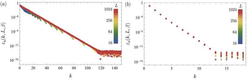
Figure 6: Additive error $\varepsilon_{a}(k,L,\beta)$, defined in Eq. (52), as a function of $k$, for $\beta=2$ and different values of $L$. In the left and right plots we report numerical data corresponding to the Ising and XXZ spin chains, respectively. The Hamiltonian parameters and bond dimensions are chosen as in Fig. 4.

In Fig. 6 we report an example of our data for $\varepsilon_{a}(k,L,\beta)$ as a function of $k$, for increasing system sizes. From the plots, two things are apparent. First, for fixed $L$, the additive error displays a clear exponential decay. Second, its values are independent of $L$ (for values of $k$ much smaller than the system size). This behavior is perfectly consistent with Eq. (33). Note that, as in the previous plots, we observe irregular behavior for sufficiently large $k$, where $\varepsilon_{a}$ approaches a plateau and displays a $L$-dependence. We interpret these effects as arising due to numerical inaccuracies (note the very small values of $\varepsilon_{a}$). Similarly, when $k$ approaches $L/2$ we observe $L$-dependent behavior, which can be attributed to finite size effects. We have repeated our calculations for different $\beta$ and Hamiltonian parameters (in each case, we have checked that the bond dimension was large enough), always finding consistent results.

V Mixed-state entanglement detection

In this section we study the $p_{n}$-PPT conditions for states satisfying the AFCs. In Sec. V.1 we first introduce a set of quantities, which we call $f_{n}(\rho)$, displaying the following properties: (i) $f_{n}(\rho)<0$ if and only if $\rho$ violates the $p_{n}$-PPT conditions and $(ii)$ $f_{n}(\rho)$ can be estimated efficiently if $\rho$ satisfies the AFCs, representing natural probes for mixed-state entanglement. Next, in Sec. V.2, we compute $f_{n}$ in a few concrete cases including Gibbs states of local Hamiltonians, and identify the values of the system parameters for which $f_{2},f_{3}<0$. The results of this section show that our approach can be successful in detecting entanglement even for large numbers of qubits and highly mixed states, thus being practically useful in many situations routinely encountered in available quantum platforms.

V.1 The $p_{n}$-PPT conditions and mixed-state entanglement probes

Given the density matrix $\rho_{AB}$ on a bipartite system, its logarithmic negativity (3) can be extracted from the knowledge of all PT moments $p_{n}$, with $n=1,\ldots,{\rm dim}(\mathcal{H}_{A}\otimes\mathcal{H}_{B})$. Therefore, while our method is efficient to estimate the individual PT moments, reconstructing the logarithmic negativity is still hard, as it requires an exponential number of them.

Luckily, the $p_{n}$-PPT conditions introduced in Sec. II.1 allow us to detect mixed-state entanglement from only a few PT moments. For example, the first two non-trivial elements in the family (5) only involve the PT moments up to $n=5$. Explicitly, they read

$$p_{3}{\rm-PPT}: \quad p_{3}p_{1}\geq p_{2}^{2}\,,$$ (53a)

$$p_{5}{\rm-PPT}: \quad p_{3}p_{5}\geq p_{4}^{2}\,.$$ (53b)

The conditions (53) can be equivalently rewritten in terms of the quantities

$$f_{3}(\rho_{AB}) =\tilde{p}_{3}\tilde{p}_{1}-\tilde{p}_{2}^{2}\frac{\mathcal{P}_{2}^{2}[A]\mathcal{P}_{2}^{2}[B]}{\mathcal{P}_{1}[A]\mathcal{P}_{1}[B]\mathcal{P}_{3}[A]\mathcal{P}_{3}[B]}\,,$$ (54a)

$$f_{5}(\rho_{AB}) =\tilde{p}_{5}\tilde{p}_{3}-\tilde{p}_{4}^{2}\frac{\mathcal{P}_{4}^{2}[A]\mathcal{P}_{4}^{2}[B]}{\mathcal{P}_{3}[A]\mathcal{P}_{3}[B]\mathcal{P}_{5}[A]\mathcal{P}_{5}[B]}\,,$$ (54b)

where $\tilde{p}_{n}$ are the normalized PT moments defined in Eq. (24). Indeed $f_{3}$ and $f_{5}$ are negative if and only if the inequalities (53) are violated.

Crucially, $f_{3}(\rho_{AB})$ and $f_{5}(\rho_{AB})$ can be estimated efficiently if $\rho_{AB}$ satisfies the AFCs. Indeed, they only depend on $\mathcal{P}_{n}$ and the normalized PT moments $\tilde{p}_{n}$, both of which can be estimated using the protocol introduced in Sec. IV. We note that such estimation protocols allow us to reconstruct $f_{n}(\rho_{AB})$ up to any arbitrary small additive error. Namely, for any arbitrary positive constant $\delta$, one can construct an estimator $f^{(e)}_{n}$, with $|f^{(e)}_{n}-f_{n}|\leq\delta$ by polynomially many (in $L$) measurements and post-processing operations. This is easily seen recalling that $\tilde{p}_{n}$ ($\mathcal{P}_{n}$) can be estimated up to any additive (relative) error, and using that

$$|\tilde{p}_{n}[I]|\leq 1\,,\qquad\frac{(\mathcal{P}_{n}[I])^{2}}{\mathcal{P}_{n-1}[I]\mathcal{P}_{n+1}[I]}\leq 1\,,$$ (55)

where the first inequality from $|\tilde{p}_{n}[I]|\leq\tilde{p}_{2}[I]=\mathcal{P}_{2}[I]$, while the second follows from Hölder’s inequality.

At this point, it is important to ask whether the quantities $f_{n}$ are practically useful in the many-body context considered in this work. For example, one could be worried that the conditions (53) are never violated for large $L$ (even if the logarithmic negativity is non-zero), or that $f_{n}$ is exponentially small in $L$ for highly mixed states, thus requiring an exponential accuracy for its estimation. To address this question, consider a family of states $\rho^{(L)}_{AB}$, defined for increasing system sizes $L$ and satisfying the AFCs. Suppose that we extract $f_{n}(\rho^{(L)}_{AB})$ using our estimation protocol for a fixed approximation error $\delta_{n}$. Then, the $p_{n}$-PPT conditions (53) allow us to successfully detect entanglement if

$$f_{3}(\rho^{(L)}_{AB}) \leq-C_{3}\,,$$ (56a)

$$f_{5}(\rho^{(L)}_{AB}) \leq-C_{5}\,,$$ (56b)

where $C_{3},C_{5}>0$ are constants (independent of $L$) with $C_{n}\geq 2\delta_{n}$. Indeed, in these cases the statistical inaccuracy is smaller (with high probability) than the amount by which $f_{n}(\rho^{(L)}_{AB})$ is negative, allowing us to certify entanglement.

In the next subsection, we study a few natural examples of states satisfying the AFCs showing that (56) hold either for all values of $L$ or up to very large system sizes. Therefore, we exhibit concrete examples where $f_{n}$ are provably useful for entanglement detection.

V.2 Mixed-state entanglement detection in FDQC and Gibbs states

We start by studying the relations (56) in the simplest case of FDQC states (13). We consider a family of states where the single-qubit density matrices in Eq. (13) are parametrized as

$$\sigma_{i}(\gamma)=\gamma\ket{a_{i}}\bra{a_{i}}+(1-\gamma)\ket{b_{i}}\bra{b_{i}}\,.$$ (57)

Here $\ket{a_{i}}$, $\ket{b_{i}}$ are arbitrary orthonormal states, while $0\leq\gamma\leq 1/2$ plays the role of a depolarizing parameter, controlling both purity and bipartite entanglement. We ask for which values of $\gamma$ the conditions (53) are violated.

This problem is analyzed in detail in Appendix F. We prove that, for generic choices of the unitary gates, there exist $\gamma_{3},\gamma_{5}>0$ such that Eqs. (56a) and  (56b) are satisfied, respectively, for all $\gamma\leq\gamma_{3}/L$ and $\gamma\leq\gamma_{5}/L^{1/3}$. Now, choosing in particular $\gamma_{L}=\gamma_{5}/L^{1/3}$, we have

$${\rm Tr}[\rho^{(L)}(\gamma_{L})^{2}] =[\gamma_{L}^{2}+(1-\gamma_{L})^{2}]^{L}$$

$$\leq\exp\left[-2(\gamma_{L}-\gamma_{L}^{2})L\right]$$

$$\leq\exp\left[-\gamma_{L}L\right]=\exp\left[-\gamma_{5}L^{2/3}\right]\,,$$ (58)

namely

$$S_{2}[\rho^{(L)}(\gamma_{L})]\geq\gamma_{5}L^{2/3}\,.$$ (59)

Therefore, $\rho^{(L)}(\gamma_{L})$ provides an example where the $p_{5}$-PPT condition is violated by a finite amount $C_{5}$ and, at the same time, the global Rényi-$2$ entropy grows polynomially, albeit sub-linearly, in the system size.

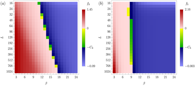
Figure 7: Density plots for the coefficients $f_{3}(\beta,L)$, $f_{5}(\beta,L)$, defined in Eq. (54) as a function of $\beta$ and $L$. The data correspond to thermal states in the Ising model (46), with $h_{x}=1.1$ and $h_{z}=-0.04$. Red (blue) regions indicate the values of $\beta$ and $L$ for which $f_{3}(\beta,L)$, $f_{5}(\beta,L)$ are larger (smaller) than some small values $-C_{3}=0.01$ and $-C_{5}=0.001$, respectively.

As a final interesting example, let us consider once again finite-temperature states of local Hamiltonians. In this case, the purity decays exponentially in $L$ and we expect that the conditions (54) fail to detect the presence of entanglement in the thermodynamic limit. In the following we give evidence that they can nevertheless be useful when considering systems of large but finite size.

To support this claim, we study thermal states in the Ising model (46), and numerically compute the coefficients (56) for different temperatures and system sizes. The computations are performed using tensor-network methods, following the same strategy explained in Sec. IV.4. An example of our results is reported in Fig. 7. In these plots, we have fixed small but otherwise arbitrary positive numbers $C_{3}$ and $C_{5}$, and identified the values of $\beta$ and $L$ for which $f_{3}(\beta,L)\leq-C_{3}$ and $f_{5}(\beta,L)\leq-C_{5}$.

The data corresponding to the $p_{3}$-PPT condition are reported in the left plot, which clearly shows that the values of the temperature $T=\beta^{-1}$ for which the entanglement can be detected decrease with $L$, consistent with our previous analysis on FDQC states. On the other hand, the right plot shows that $f_{5}(\beta,L)<-C_{5}$ up to values of the temperature ($T\simeq 0.1)$ that do not significantly depend on $L$, at least up to very large system sizes ($L\simeq 1024$). We expect that this is a finite-size effect, namely that increasing $L$ further, the values of $T$ for which entanglement can be detected will decrease. Still, this example shows how the $p_{n}$-PPT conditions may be able to detect entanglement even for highly mixed states and up to very large system sizes, making the estimation protocol for PT moments practically very useful.

VI Outlook

We have studied the problem of estimating global entropies and entanglement in many-qubit states, assuming the validity of certain AFCs which encode the fact that all the spatial correlations lengths in the system are finite. We have shown that the AFCs allow one to reconstruct entropies and PT moments from local information which can be extracted efficiently using standard RM schemes. Exploiting this fact, we have devised a very simple strategy for entropy and entanglement estimation which is provably accurate, requiring polynomially-many local measurements and post-processing operations. We have discussed the generality of the AFCs, providing both analytic and numerical evidence for their validity in different classes of states, including MPDOs and thermal states of local Hamiltonians.

As we have argued, the protocols proposed in this work could be practically useful to detect bipartite mixed-state entanglement for large numbers of qubits in today’s quantum platforms. This is especially true when considering current NISQ devices from the point of view of quantum simulation, since the AFCs hold under assumptions that are very common in the context of many-body physics. In addition, our work also raises important questions and opens up a number of interesting directions.

First, our protocols assume that the state to be measured satisfies the AFCs. Therefore, an important question from the experimental perspective is whether it is possible to devise a complementary (and still efficient) strategy to certify their validity, similar to what can be done in the case of MPS Cramer et al. (2010) or entanglement-Hamiltonian tomography Joshi et al. (2023).

As we have discussed in Sec. IV.1, a simple but effective consistency check can be carried out by repeating our protocols multiple times, each time with an increased ansatz value for the correlation lengths. If the estimated purities or PT moments change beyond the expected precision over different repetitions, we obtain a “red flag” signalling the failure of the AFCs in the state to be measured. This process, however, does not allow one to rigorously rule out the presence of long-range correlations, as this would require running the estimation protocols using, as an input, correlation lengths which are proportional to the system size. We envision that a way to tackle the certification problem could be to identify a hierarchy of properties which are strictly stonger than the AFCs and for which rigorous certification protocols can be found more easily. At the moment, however, this remains an open problem.

Next, while we have focused on $1D$ systems, a very natural direction is to extend our approach to higher spatial dimensions. In this case, additional technical complications arise, but we expect that efficient estimation strategies for the purity and PT moments exists under similar conditions encoding the absence of long-range correlations. We stress that this problem is particularly important, since tomographic methods for many-qubit states (based, for instance on tensor or neural networks) are much less developed in higher dimensions.

Finally, we mention that our approach could also be applied to probe other quantities which generally require exponentially many measurements. Straightforward examples include the participation entropies Luitz et al. (2014); Stéphan et al. (2009, 2010); Alcaraz and Rajabpour (2013); Stéphan (2014) and the so-called stabilizer Rényi entropies Leone et al. (2022), but we expect that similar ideas could be implemented in other contexts. One example is that of cross-platform verification protocols Elben et al. (2020b), which involve probing the (possibly exponentially small) overlaps between different density matrices. Similarly, efficient estimation strategies for the so-called Loschmidt echo Quan et al. (2006) also appear to be within the reach of the techniques developed in this work. While these problems require dealing with additional technical subtleties compared to the analysis of the entropy and PT moments, we believe that the latter are not substantial and could be overcome. We leave the study of these applications to future research.

Appendix A Factorization condition for FDQC states

A.1 The purity

In this Appendix we show that the FDQC states (13) satisfy the factorization condition (14). In fact, we prove the stronger condition

$${\rm Tr}_{B^{\otimes n}}\left[\overrightarrow{\Pi}_{B}\left(\rho_{ABC}^{\otimes n}\right)\right]\qquad$$

$$=\frac{{\rm Tr}_{B^{\otimes n}}\left[\overrightarrow{\Pi}_{B}\left(\rho_{AB}^{\otimes n}\right)\right]\otimes{\rm Tr}_{B^{\otimes n}}\left[\overrightarrow{\Pi}_{B}\left(\rho_{BC}^{\otimes n}\right)\right]}{{\rm Tr}_{B}(\rho_{B}^{n})}\,,$$ (60)

where we introduced the $n$-copy cyclic permutation operator $\overrightarrow{\Pi}_{B}\ket{i_{1},\ldots i_{n}}=\ket{i_{n},i_{1},\ldots i_{n-1}}$, and we assumed $|B|\geq(2\ell-1)$, where $\ell$ is the circuit depth. We make use of a graphical derivation. We show the case $n=2$, $\ell=4$, and $|B|=8$ for concreteness, but it is clear that the proof generalizes for all values of $n$ and $\ell$. The reduced density matrix over the interval $\mathcal{I}=A\cup B\cup C$ reads

(61)

Following the standard tensor-network notation, lower (upper) dangling legs correspond to the input (output) qubits. In addition, here and in the following upper and lower legs in the same column which are marked with a small rectangle of the same color are traced over. Finally, black dots correspond to the density matrices $\sigma_{j}$.

The left-hand side of Eq. (A.1) can be represented as

(62)

where dangling legs are not contracted, while the gray rectangle is a short-hand notation for the reduced density matrix (61). Using unitarity of the gates, we get ${\rm Tr}_{B^{\otimes n}}\left[\overrightarrow{\Pi}_{B}\left(\rho_{ABC}^{\otimes n}\right)\right]=T_{1}T_{2}T_{3}$, where

Note that $T_{1}$ and $T_{3}$ are operators, while $T_{2}$ is a number. Let us compare this graphical expression with the one in the RHS of Eq. (A.1). The first and second terms in the numerator read, respectively

$$\raisebox{-68.0pt}{\includegraphics[scale={0.24}]{identity2.pdf}}\,.$$

Similarly, the denominator in Eq. (A.1) reads

Putting everything together, and simplifying the common factors in the numerator and denominator, we arrive at Eq. (A.1). Finally, using the fact that $\operatorname{Tr}(\rho_{X}^{n})=\operatorname{Tr}(\overrightarrow{\Pi}_{X}\rho_{X}^{\otimes n})$, and the relation $\overrightarrow{\Pi}_{ABC}=\overrightarrow{\Pi}_{A}\otimes\overrightarrow{\Pi}_{B}\otimes\overrightarrow{\Pi}_{C}$, we arrive at

$${\rm Tr}(\rho_{ABC}^{n})=\frac{{\rm Tr}_{AB}(\rho_{AB}^{n}){\rm Tr}_{BC}(\rho_{BC}^{n})}{{\rm Tr}_{B}(\rho_{B}^{n})}\,.$$ (63)

For $n=2$, this proves Eq. (14).

Next, we prove Eq. (15). Let us consider a partition of the whole system $\mathcal{S}=A\cup B\cup C$, where $|B|=|C|=k\geq 2\ell-1$. We first make use of Eq. (14). Setting now $A^{(0)}:=A$, $B^{(0)}:=B$, $C^{(0)}:=C$ we can iterate this operation, each time splitting the interval $A^{(j)}\cup B^{(j)}$ into three adjacent regions $A^{(j+1)}$, $B^{(j+1)}$, and $C^{(j+1)}$ with $|B^{(j+1)}|=|C^{(j+1)}|=k$. We continue this procedure until $|A^{R}|=k$, which gives us Eq. (15).

A.2 The PT moments

The goal of this Appendix is to prove Eq. (25).

We start by recalling the expression for the PT moments Carteret (2005)

$${\rm Tr}\left[\left(\rho_{AB}^{T_{A}}\right)^{n}\right] ={\rm Tr}\left[\overleftarrow{\Pi}_{A}\overrightarrow{\Pi}_{B}\left(\rho_{AB}^{\otimes n}\right)\right],$$ (64)

where we introduced the $n$-copy forward (backward) cyclic permutation operator in the $n$-replica space, defined by

$$\overrightarrow{\Pi}_{A}\ket{i_{1},\ldots i_{n}} =\ket{i_{n},i_{1},\ldots i_{n-1}}\,,$$

$$\overleftarrow{\Pi}_{B}\ket{i_{1},\ldots i_{n}} =\ket{i_{2},i_{3},\ldots i_{1}}\,.$$ (65)

Using this notation, it is easy to see that Eq. (A.1) implies

$${\rm Tr}_{B^{\otimes n}}\left[\overleftarrow{\Pi}_{B}\left(\rho_{ABC}^{\otimes n}\right)\right]=$$

$$\frac{{\rm Tr}_{B^{\otimes n}}\left[\overleftarrow{\Pi}_{B}\left(\rho_{AB}^{\otimes n}\right)\right]\otimes{\rm Tr}_{B^{\otimes n}}\left[\overleftarrow{\Pi}_{B}\left(\rho_{BC}^{\otimes n}\right)\right]}{{\rm Tr}_{B}(\rho_{B}^{n})}\,,$$ (66)

Eq. (A.2) can be proved by taking the partial-transpose with respect to $A^{\otimes n}$ and $C^{\otimes n}$ in both sides of (A.1), followed by complex conjugation. Next, let us take a bipartition of the system into $A$ and $B$, each divided into two intervals $A=A_{1}\cup A_{2}$ and $B=B_{1}\cup B_{2}$ with $|A_{2}|=|B_{1}|=k$, cf. Fig. 3$(b)$. Making use of Eq. (A.1), we have

$${\rm Tr}\left[\left(\rho_{AB}^{T_{A}}\right)^{n}\right] ={\rm Tr}_{A^{\otimes n}}{\rm Tr}_{B_{2}^{\otimes n}}\overleftarrow{\Pi}_{A}\overrightarrow{\Pi}_{B_{2}}{\rm Tr}_{B_{1}^{\otimes n}}\overrightarrow{\Pi}_{B_{1}}\rho^{\otimes n}$$

$$=\frac{{\rm Tr}_{A^{\otimes n}\otimes B_{1}^{\otimes n}}(\overleftarrow{\Pi}_{A}\overrightarrow{\Pi}_{B_{1}}\rho_{AB_{1}}^{\otimes n})}{{\rm Tr}_{B_{1}}(\rho_{B_{1}}^{n})}$$

$$\times\frac{{\rm Tr}_{B_{1}^{\otimes n}\otimes B_{2}^{\otimes n}}(\vec{\Pi}_{B_{1}}\vec{\Pi}_{B_{2}}\rho_{B_{1}B_{2}}^{\otimes n})}{{\rm Tr}_{B_{1}}(\rho_{B_{1}}^{n})}\,.$$ (67)

Using

$${\rm Tr}_{A^{\otimes n}\otimes B_{1}^{\otimes n}}(\overleftarrow{\Pi}_{A}\overrightarrow{\Pi}_{B_{1}}\rho_{AB_{1}}^{\otimes n})$$

$$={\rm Tr}_{A_{1}^{\otimes n}}{\rm Tr}_{B_{1}^{\otimes n}}\overleftarrow{\Pi}_{A_{1}}\overrightarrow{\Pi}_{B_{1}}{\rm Tr}_{A_{2}^{\otimes n}}\overleftarrow{\Pi}_{A_{2}}\rho_{A_{1}A_{2}B_{1}}^{\otimes n}$$

$$={\rm Tr}_{A_{1}^{\otimes n}\otimes A_{2}^{\otimes n}}(\overleftarrow{\Pi}_{A_{1}}\overleftarrow{\Pi}_{A_{2}}\rho_{A_{1}A_{2}}^{\otimes n})$$

$${\rm Tr}_{A_{2}^{\otimes n}\otimes B_{1}^{\otimes n}}(\overleftarrow{\Pi}_{A_{2}}\overrightarrow{\Pi}_{B_{1}}\rho_{A_{2}B_{1}}^{\otimes n})\left[{\rm Tr}_{A_{2}}(\rho_{A_{2}}^{n})\right]^{-1}\,,$$ (68)

we finally arrive at Eq. (25).

Appendix B Statistical-error analysis in FDQC states

B.1 Statistical-error analysis for the purity

In this Appendix we prove Eq. (20). We consider the protocol explained in Sec. III.1 and denote by $\mathcal{P}^{(e)}_{2}[I]$ the estimates for $\mathcal{P}_{2}[I]={\rm Tr}(\rho_{I}^{2})$ obtained from the classical-shadow approach. These local purities are estimated with a non-zero relative error, i.e. $\mathcal{P}_{2}^{(e)}[I]/\mathcal{P}_{2}[I]=(1+\varepsilon^{I})$. We define

$$\varepsilon={\rm max}\left\{|\varepsilon^{I}|:I\in\{I_{j}\}_{j}\cup\{I_{j}\cup I_{j+1}\}_{j}\right\}\,.$$ (69)

We will take $r^{(e)}_{2}$, defined in Eq. (17), as the experimental estimate for the global purity $\mathcal{P}_{2}={\rm Tr}(\rho^{2})$, choosing the intervals $I_{j}$ with $|I_{j}|=k\geq 2\ell-1$, where $\ell$ is the circuit depth, so that Eq. (15) holds.

We start our proof from a few preliminary lemmas.

Lemma 1.

Suppose $\varepsilon\leq 1/2$. Then

$$\left|\frac{r_{2}^{(e)}}{\mathcal{P}_{2}}-1\right|\leq e^{(4L/k)\varepsilon}-1\,.$$ (70)

Proof.

Setting $\mathcal{P}_{2}^{(e)}[I]=\mathcal{P}_{2}[I](1+\varepsilon^{I}$),recalling $R=L/k$, where $k=|I_{j}|$ and using (15), we have

$$\frac{r_{2}^{(e)}}{\mathcal{P}_{2}}=\frac{\prod_{j=1}^{R-1}(1+\varepsilon^{I_{j}\cup I_{j+1}})}{\prod_{j=2}^{R-1}(1+\varepsilon^{I_{j}})}\,,$$ (71)

as so, using $|\varepsilon^{I}|\leq\varepsilon$,

$$\frac{r_{2}^{(e)}}{\mathcal{P}_{2}} \leq\frac{(1+\varepsilon)^{R-1}}{(1-\varepsilon)^{R-2}}\leq\left[\frac{1+\varepsilon}{1-\varepsilon}\right]^{R}\,,$$

$$\frac{r_{2}^{(e)}}{\mathcal{P}_{2}} \geq\frac{(1-\varepsilon)^{R-1}}{(1+\varepsilon)^{R-2}}\geq\left[\frac{1-\varepsilon}{1+\varepsilon}\right]^{R}\,.$$ (72)

Since $\varepsilon\leq 1/2$, and using $(1+x)\leq e^{x}$, we have

$$\frac{1+\varepsilon}{1-\varepsilon}=1+\frac{2\varepsilon}{1-\varepsilon}\leq 1+4\varepsilon\leq e^{4\varepsilon}\,.$$ (73)

Therefore,

$$e^{-(4L/k)\varepsilon}\leq\frac{r_{2}^{(e)}}{\mathcal{P}_{2}}\leq e^{(4L/k)\varepsilon}\,.$$ (74)

Finally, using

$$(1-e^{-a})\leq e^{a}-1\,,$$ (75)

we obtain (70) ∎

Lemma 2.

Let $M\geq 2^{4|I|}$. Then

$${\rm Pr}\left(|\varepsilon^{I}|\geq\alpha\right)\leq\frac{2^{2|I|+3}}{\alpha^{2}M}\,.$$ (76)

Proof.

We start from the bound (10). Since $M\geq 2^{4|I|}$, we have in particular $M\geq 4$ and Eq. (10) implies

$${\rm Var}\left[\mathcal{P}_{2}^{(e)}[I]\right] \leq 4\left(\frac{2^{|I|}\mathcal{P}_{2}[I]}{M}\right)+4\left(\frac{2^{2|I|}}{M}\right)^{2}\,.$$ (77)

Since by hypothesis $M\geq 2^{4|I|}$, while $\mathcal{P}_{2}[I]\geq 2^{-|I|}$, we have

$$4\left(\frac{2^{2|I|}}{M}\right)^{2}\leq 4\left(\frac{2^{|I|}\mathcal{P}_{2}[I]}{M}\right),$$ (78)

and so

$${\rm Var}\left[\mathcal{P}_{2}^{(e)}[I]\right]\leq 8\frac{2^{|I|}\mathcal{P}_{2}[I]}{M}\,.$$ (79)

Eq. (76) then follows using Chebyshev’s inequality and $\mathcal{P}_{2}[I]\geq 2^{-|I|}$. ∎

We are ready to state and prove the main result of this section.

Theorem 1.

Let $0\leq\delta\leq 1$ and take

$$M\geq{\rm max}\left\{2^{8k},L^{2}\frac{2^{4k+10}}{k^{2}\delta^{2}}\right\}\,,$$ (80)

where $k=|I_{j}|\geq 2$ (the case $k=1$ is trivial). Then

$${\rm Pr}\left[\left|(r_{2}^{(e)}/\mathcal{P}_{2})-1\right|\geq\delta\right]\leq\frac{2^{4k+11}L^{3}}{\delta^{2}k^{3}M}\,.$$ (81)

Proof.

Recalling the definition (69), note that if $\varepsilon<(k/8L)\delta$, then $\varepsilon<1/2$ and also $e^{(4L/k)\varepsilon}-1<\delta$. Using Lemma 1, this implies

$${\rm Pr}\left[\left|(r_{2}^{(e)}/\mathcal{P}_{2})-1\right|\right. \left.\geq\delta\right]\leq{\rm Pr}[\varepsilon\geq(k/8L)\delta]$$

$$=1-{\rm Pr}[\varepsilon<(k/8L)\delta]\,.$$ (82)

In more detail, the validity of the first inequality can be seen as follows: Suppose $\varepsilon<(k/8L)\delta$. Then necessarily $\varepsilon<1/2$ and so also $|r^{(e)}_{2}/\mathcal{P}_{2}-1|<\delta$ (by Lemma 1). Therefore, the set of cases in which $|r^{(e)}_{2}/\mathcal{P}_{2}-1|\geq\delta$ must be contained in the set of cases in which $\varepsilon\geq(k/8L)\delta$. In formula, this is the first line of Eq. (B.1).

From the definition of $\varepsilon$ and Lemma 2, we have

$${\rm Pr}[\varepsilon<x] =\prod_{j}\left(1-{\rm Pr}[|\varepsilon^{I_{j}}|\geq x]\right)$$

$$\times\prod_{j}\left(1-{\rm Pr}[|\varepsilon^{I_{j}\cup I_{j+1}}|\geq x]\right)$$

$$\geq\left[\left(1-\frac{2^{2k+3}}{x^{2}M}\right)\left(1-\frac{2^{4k+3}}{x^{2}M}\right)\right]^{R}\,,$$ (83)

where we used that the random variables $\varepsilon^{I_{j}}$ are statistically independent. Therefore

$${\rm Pr}[\varepsilon<x]\geq\left(1-\frac{2^{4k+3}}{x^{2}M}\right)^{2R}\,.$$ (84)

Setting $x=\delta k/(8L)$, we have by hypothesis $2^{4k+3}/x^{2}M\leq 1/2$. Therefore, using $1-z\geq e^{-2z}$ for $0\leq z\leq 1/2$, we obtain

$${\rm Pr}[\varepsilon<(k/8L)\delta]\geq\exp\left[-\frac{2^{4k+11}L^{3}}{M\delta^{2}k^{3}}\right]\,.$$ (85)

Plugging this into (B.1), and using $1-e^{-z}\leq z$, we finally obtain (81). ∎

B.2 Statistical-error analysis for the PT moments

In this Appendix we prove Eq. (31). Considering the same protocol and using the same notation as Sec. III.2, we set

$$p_{3}^{(e)}[A_{2}B_{1}] =p_{3}[A_{2}B_{1}]+\varepsilon^{A_{2}B1}\,,$$ (86a)

$$\mathcal{P}_{3}^{(e)}[A_{2}] =\mathcal{P}_{3}[A_{2}](1+\varepsilon^{A_{2}})\,,$$ (86b)

$$\mathcal{P}_{3}^{(e)}[B_{1}] =\mathcal{P}_{3}[B_{1}](1+\varepsilon^{B_{1}})\,.$$ (86c)

Note that $\varepsilon^{A_{2}B_{1}}$ is an additive error, while $\varepsilon^{A_{2}}$, $\varepsilon^{B_{1}}$ are relative errors. We also define

$$\varepsilon=2^{2|A_{2}|+2|B_{1}|}{\rm max}\left\{|\varepsilon^{A_{2}B_{1}}|,|\varepsilon^{A_{2}}|,|\varepsilon^{B_{1}}|\right\}\,.$$ (87)

In the following, we will set $|A_{2}|=|B_{1}|=k$, where $k\geq 2\ell-1$ with $\ell$ being the circuit depth. With this choice, Eq. (26) holds.

For clarity, we organize the proof into lemmas.

Lemma 3.

Suppose $\varepsilon\leq 1$. Then

$$\left|s_{3}^{(e)}[A_{2}B_{1}]-s_{3}[A_{2}B_{1}]\right|\leq 16\varepsilon\,,$$ (88)

where $s_{n}[A_{2}B_{1}]$ is defined in Eq. (26).

Proof.

We start from

$$s^{(e)}_{3}[A_{2}B_{1}] =\frac{p_{3}[A_{2}B_{1}]+\varepsilon^{A_{2}B_{1}}}{\mathcal{P}_{3}[A_{2}](1+\varepsilon^{A_{2}})\mathcal{P}_{3}[B_{1}](1+\varepsilon^{B_{1}})}\,,$$ (89)

which gives us

$$|s^{(e)}_{3}[A_{2}B_{1}]-s_{3}[A_{2}B_{1}]|\leq$$

$$\frac{|p_{3}[A_{2}B_{1}]|}{\mathcal{P}_{3}[A_{2}]\mathcal{P}_{3}[B_{1}]}\frac{|\varepsilon^{A_{2}}|+|\varepsilon^{B_{1}}|+|\varepsilon^{A_{2}}\varepsilon^{B_{1}}|}{(1+\varepsilon^{A_{2}})(1+\varepsilon^{B_{1}})}$$

$$+\frac{|\varepsilon^{A_{2}B_{1}}|}{\mathcal{P}_{3}[A_{2}]\mathcal{P}_{3}[B_{1}](1+\varepsilon^{A_{2}})(1+\varepsilon^{B_{1}})}\,.$$ (90)

Denoting by $\lambda_{j}$ the eigenvalues of $\rho^{T_{A_{2}}}_{A_{2}B1}$, we have

$$|p_{3}[A_{2}B_{1}]|\leq\sum_{j}|\lambda_{j}|^{3}\leq\sum_{j}\lambda_{j}^{2}=\mathcal{P}[A_{2}B_{1}]\leq 1\,,$$ (91)

where we used $\lambda_{j}\in[-1/2,1]$ Rana (2013) and ${\rm Tr}[(\rho_{AB}^{T_{A}})^{2}]={\rm Tr}[\rho_{AB}^{2}]$ Elben et al. (2020a). In addition, since $\varepsilon\leq 1$, clearly $|\varepsilon^{A_{2}}|\leq 1/2$, $|\varepsilon^{B_{1}}|\leq 1/2$ and so also $|\varepsilon^{A_{2}}\varepsilon^{B_{1}}|<|\varepsilon^{A_{2}}|$. Putting everything together, and using $\mathcal{P}_{3}[I]\leq 2^{-2|I|}$, we finally arrive at Eq. (88). ∎

Lemma 4.

Let $M\geq 3\cdot 2^{8k}$. Then

$${\rm Pr}\left(|\varepsilon^{A_{2}}|\geq\alpha\right) \leq 27\frac{2^{3k}}{\alpha^{2}M}\,,$$ (92a)

$${\rm Pr}\left(|\varepsilon^{B_{1}}|\geq\alpha\right) \leq 27\frac{2^{3k}}{\alpha^{2}M}\,,$$ (92b)

$${\rm Pr}\left(|\varepsilon^{A_{2}B_{1}}|\geq\alpha\right) \leq 27\frac{2^{2k}}{\alpha^{2}M}\,.$$ (92c)

Proof.

We start from the bound Rath et al. (2021a)

$$\operatorname{Var}\left[p^{(e)}_{3}[AB]\right] \leq 9\frac{2^{|AB|}}{M}\operatorname{Tr}\left(\rho_{AB}^{4}\right)$$

$$+ 18\frac{2^{3|AB|}}{(M-1)^{2}}p_{2}[AB]+6\frac{2^{6|AB|}}{(M-2)^{3}}\,.$$ (93)

Since $M\geq 3\cdot 2^{8k}$ (and $k\geq 1$), then

$$\frac{18}{(M-1)^{2}}\leq\frac{27}{M^{2}}\,,\quad\frac{6}{(M-2)^{3}}\leq\frac{9}{M^{3}}\,.$$ (94)

Therefore

$$\operatorname{Var}\left[p^{(e)}_{3}[AB]\right] \leq 9\frac{2^{|AB|}}{M}\operatorname{Tr}\left(\rho_{AB}^{4}\right)$$

$$+ 27\frac{2^{3|AB|}}{M^{2}}p_{2}[AB]+9\frac{2^{6|AB|}}{M^{3}}\,.$$ (95)

Since $M\geq 3\cdot 2^{8k}$, we have

$$9\frac{2^{|AB|}}{M}\operatorname{Tr}\left(\rho_{AB}^{4}\right) \geq 27\frac{2^{3|AB|}}{M^{2}}p_{2}[AB]\,,$$

$$9\frac{2^{|AB|}}{M}\operatorname{Tr}\left(\rho_{AB}^{4}\right) \geq 9\frac{2^{6|AB|}}{M^{3}}\,.$$ (96)

In the first line we have used that $p_{2}[I]={\rm Tr}[\rho_{I}^{2}]$ and Hölder’s inequality, which guarantees

$${\rm Tr}[\rho^{2}_{I}]/{\rm Tr}[\rho^{4}_{I}]\leq 2^{|I|}/{\rm Tr[\rho_{I}^{2}]}\leq 2^{2|I|}\,,$$ (97)

while in the second line we have used ${\rm Tr}(\rho_{AB}^{4})\geq 2^{-3|AB|}=2^{-6k}$. Putting all together, we get

$$\operatorname{Var}\left[p^{(e)}_{3}[AB]\right]\leq 27\frac{2^{2k}}{M}\operatorname{Tr}\left(\rho_{AB}^{4}\right)\,.$$ (98)

Similarly, we have Rath et al. (2021a)

$$\operatorname{Var}\left[\mathcal{P}_{3}[A_{2}]\right] \leq 9\frac{2^{|A_{2}|}}{M}\operatorname{Tr}\left(\rho_{A_{2}}^{4}\right)$$

$$+ 18\frac{2^{3|A_{2}|}}{(M-1)^{2}}\operatorname{Tr}\left(\rho_{A_{2}}^{2}\right)+6\frac{2^{6|A_{2}|}}{(M-2)^{3}}$$

$$\leq 27\frac{2^{k}}{M}\operatorname{Tr}\left(\rho_{A_{2}}^{4}\right)\,.$$ (99)

Using ${\rm Tr}\left(\rho_{A_{2}}^{4}\right)/({\rm Tr}(\rho_{A_{2}}^{3}))^{2}\leq 1/{\rm Tr}(\rho_{A_{2}}^{3})\leq 2^{2k}$, we obtain

$${\rm Var}\left[\frac{\mathcal{P}^{(e)}_{3}[A_{2}]}{\mathcal{P}_{3}[A_{2}]}\right]\leq 27\frac{2^{k}}{M}\frac{{\rm Tr}\left(\rho_{A_{2}}^{4}\right)}{({\rm Tr}(\rho_{A_{2}}^{3}))^{2}}\leq 27\frac{2^{3k}}{M}\,,$$ (100)

and analogously for $\mathcal{P}^{(2)}_{3}(B_{1})$. Eqs. (92) follow using Chebyshev’s inequality. ∎

We are ready to state and prove the main result of this section, yielding Eq. (31).

Theorem 2.

Let $0\leq\delta\leq 1$ and take

$$M\geq 27\frac{2^{11k+9}}{\delta^{2}}\,.$$ (101)

Then

$${\rm Pr}\left[\left|s^{(e)}_{3}[A_{2}B_{1}]-s_{3}[A_{2}B_{1}]\right|\geq\delta\right]\leq 81\frac{2^{11k+9}}{M\delta^{2}}\,.$$ (102)

Proof.

Recall the definition (87) and note that if $\varepsilon\leq\delta/16$, then trivially $\varepsilon<1$ and so, by Lemma 3, $|s^{(e)}_{3}-s_{3}|\leq\delta$. This implies

$${\rm Pr}[|s^{(e)}_{3}-s_{3}| \geq\delta]\leq{\rm Pr}[\varepsilon\geq\delta/16]$$

$$=1-{\rm Pr}[\varepsilon<\delta/16]\,.$$ (103)

In more detail, the validity of the first inequality can be seen as follows: Suppose $\varepsilon<\delta/16$. Then trivially $\varepsilon<1$ and so necessarily also $|s^{(e)}_{3}-s_{3}|<\delta$ (by Lemma 3). Therefore, the set of cases in which $|s^{(e)}_{3}-s_{3}|\geq\delta$ is contained in the set of cases for which $\varepsilon\geq\delta/16$. In formula, this is the first line of Eq. (B.2).

From the definition of $\varepsilon$ and Lemma 4, we have

$${\rm Pr}[\varepsilon<x]=(1-{\rm Pr}[|\varepsilon^{A_{2}}|\geq x2^{-4k}])$$

$$\times(1-{\rm Pr}[|\varepsilon^{B_{1}}|\geq x2^{-4k}])(1-{\rm Pr}[|\varepsilon^{A_{2}B_{1}}|\geq x2^{-4k}])\,$$

$$\geq\left(1-27\frac{2^{11k}}{x^{2}M}\right)^{3}\,,$$ (104)

where we used that the random variables $\varepsilon^{I_{j}}$ are statistically independent. Setting $x=\delta/16$, we have by hypothesis $27\cdot 2^{11k}/x^{2}M<1/2$. Therefore, using $1-z\geq e^{-2z}$ for $0\leq z\leq 1/2$, we obtain

$${\rm Pr}[\varepsilon<\delta/16]\geq\exp\left[-81\frac{2^{11k+9}}{M\delta^{2}}\right]\,.$$ (105)

Plugging into (B.2), and using $1-e^{-z}\leq z$, we finally obtain (102). ∎

Appendix C Statistical-error analysis for states satisfying the AFCs

In this Appendix we prove the main claims reported in Sec. IV.2. Let $\rho$ be a state satisfying (32) for all partitions as in Fig. 3$(a)$, with $|B|=k\geq k_{c}$ (and open boundary conditions). We first prove Eq. (35).

We start with the following:

Lemma 5.

Let

$$k\geq\frac{\ln(\alpha_{2}L/\delta)}{\beta_{2}}\,,$$ (106)

for $0\leq\delta\leq 1/2$. Then, defining $r_{2}$ as in Eq. (36), we have

$$\left|\frac{r_{2}}{{\rm Tr}(\rho^{2})}-1\right|\leq 4\delta\,.$$ (107)

Proof.

First, applying iteratively (32), we get (recalling that $R=L/k$)

$$\frac{r_{2}}{{\rm Tr}(\rho^{2})}=\prod_{j=2}^{R-1}(1+\varepsilon_{j})\,,$$ (108)

with $|\varepsilon_{j}|\leq\alpha_{2}e^{-\beta_{2}k}$, and so

$$\left|\frac{r_{2}}{{\rm Tr}(\rho^{2})}-1\right|=\left|\prod_{j=2}^{R-1}(1+\varepsilon_{j})-1\right|\,.$$ (109)

We have

$$\prod_{j=2}^{R-1}(1+\varepsilon_{j})-1\leq(1+\alpha_{2}e^{-\beta_{2}k})^{R-2}-1$$

$$\leq\exp\left[\alpha_{2}(L/k)e^{-\beta_{2}k}\right]-1\,.$$ (110)

Analogously,

$$\prod_{j=2}^{R-1}(1+\varepsilon_{j})-1\geq(1-\alpha_{2}e^{-\beta_{2}k})^{R-2}-1\,.$$ (111)

Due to (106), we have $\alpha_{2}e^{-\beta_{2}k}\leq 1/2$. Therefore, using $1-z\geq e^{-2z}$ for $0\leq z\leq 1/2$, we have

$$\prod_{j=2}^{R-1}(1+\varepsilon_{j})-1\geq\exp\left[-2\alpha_{2}(L/k)e^{-\beta_{2}k}\right]-1\,.$$ (112)

Therefore

$$e^{-y}-1\leq\prod_{j=2}^{R-1}(1+\varepsilon_{j})-1\leq e^{y/2}-1\leq e^{y}-1\,,$$ (113)

where $y=2\alpha_{2}(L/k)e^{-\beta_{2}k}$. Since $1-e^{-y}\leq e^{y}-1$, this implies

$$\left|\prod_{j=2}^{R-1}(1+\varepsilon_{j})-1\right|\leq\exp\left[2\alpha_{2}(L/k)e^{-\beta_{2}k}\right]-1\,.$$ (114)

Finally, due to (106), we have $2\alpha_{2}(L/k)e^{-\beta_{2}k}\leq 1$. Therefore, using $e^{z}-1\leq 2z$ for $0\leq z\leq 1$, we arrive at

$$\left|\frac{r_{2}}{{\rm Tr}(\rho^{2})}-1\right|\leq\frac{4\alpha_{2}L}{k}e^{-\beta_{2}k}\leq 4\delta\,.$$ (115)

∎

Next, we prove Eq. (35), via the following:

Theorem 3.

Let $0\leq\delta\leq 1/2$ and set

$$k=\frac{\ln(\alpha_{2}L/\delta)}{\beta_{2}}\,.$$ (116)

Choosing

$$M\geq{\rm max}\left\{\left(\frac{\alpha_{2}L}{\delta}\right)^{\frac{8\ln 2}{\beta_{2}}},\frac{L^{2}2^{10}}{\delta^{2}}\left(\frac{\alpha_{2}L}{\delta}\right)^{\frac{4\ln 2}{\beta_{2}}}\right\}\,,$$ (117)

and recalling the definition (17), we have

$${\rm Pr}\left[\left|(r_{2}^{(e)}/\mathcal{P}_{2})-1\right|\geq 7\delta\right]\leq\frac{2^{11}L^{3}}{\delta^{2}M}\left(\frac{\alpha_{2}L}{\delta}\right)^{\frac{4\ln 2}{\beta_{2}}}\,.$$ (118)

Proof.

Set $r_{2}^{(e)}/r_{2}=(1+\varepsilon_{1})$ and $r_{2}/\mathcal{P}_{2}=(1+\varepsilon_{2})$, where $r^{(e)}_{2}$ is defined in Eq. (17). Using Lemma 5 (and that $\delta\leq 1/2$), we have $|\varepsilon_{2}|\leq 4\delta$ and so

$$\left|\frac{r_{2}^{(e)}}{\mathcal{P}_{2}}-1\right| =\left|\frac{r_{2}^{(e)}}{r_{2}}\frac{r_{2}}{\mathcal{P}_{2}}-1\right|\leq 4\delta+3|\varepsilon_{1}|\,.$$ (119)

If $|\varepsilon_{1}|<\delta$, then $|r^{(e)}_{2}/\mathcal{P}_{2}-1|<7\delta$. Therefore, the set of cases in which $|r^{(e)}_{2}/\mathcal{P}_{2}-1|\geq 7\delta$ is contained in the set of cases in which $|\varepsilon_{1}|\geq\delta$. In formula,

$${\rm Pr}[|(r_{2}^{(e)}/\mathcal{P}_{2})-1| \geq 7\delta]\leq{\rm Pr}[|(r_{2}^{(e)}/r_{2})-1|\geq\delta|]\,.$$ (120)

Thanks to Eq. (117), we can use Theorem 1, yielding

$${\rm Pr}[|(r_{2}^{(e)}/r_{2})-1|\geq\delta|] \leq\frac{2^{4k+11}L^{3}}{\delta^{2}k^{3}M}\leq\frac{2^{4k+11}L^{3}}{\delta^{2}M}$$

$$\leq\frac{2^{11}L^{3}}{\delta^{2}M}\left(\frac{\alpha_{2}L}{\delta}\right)^{\frac{4\ln 2}{\beta_{2}}}\,,$$ (121)

which completes the proof. ∎

Note that, in order to recover Eqs. (34) and  (35), we simply rename $\delta^{\prime}=7\delta$.

Finally, we present a technical result showing that the PT moments can be estimated efficiently, assuming that the state to be measured satisfies the AFCs. We focus for simplicity on the case $n=3$ and follow a protocol similar to that of Sec. III.2. Namely, we take $s^{(e)}_{3}[A_{2}B_{1}]$, defined in (28), as our estimator for $\tilde{p}_{3}[AB]$, and, for any $0\leq\delta\leq 1$, we choose

$$k=\frac{\ln(2\alpha_{3}/\delta)}{2\beta_{3}}\,.$$ (122)

Finally, we perform $M$ measurements to estimate $p_{3}[A_{2}B_{1}]$, $\mathcal{P}_{3}[A_{2}]$, and $\mathcal{P}_{3}[B_{1}]$ each (so the total number is $M_{T}=3M$). We can then prove the following:

Theorem 4.

For any $0\leq\delta\leq 1/2$, set

$$k=\frac{\ln(2\alpha_{3}/\delta)}{2\beta_{3}}\,.$$ (123)

If

$$M\geq 27\frac{2^{9}}{\delta^{2}}\left(\frac{2\alpha_{3}}{\delta}\right)^{\frac{11\ln 2}{2\beta_{3}}}\,,$$ (124)

then

$${\rm Pr}\left[\left|s^{(e)}_{3}-\tilde{p}_{3}\right|\geq\delta\right]\leq\frac{81\cdot 2^{9}}{\delta^{2}M}\left(\frac{2\alpha_{3}}{\delta}\right)^{\frac{11\ln 2}{2\beta_{3}}}\,.$$ (125)

Proof.

Our estimator for the normalized PT moment $\tilde{p}_{3}[AB]$ is

$$s^{(e)}_{3}=\frac{p^{(e)}_{3}[A_{2}B_{1}]}{\mathcal{P}^{(e)}_{3}[A_{2}]\mathcal{P}^{(e)}_{3}[B_{1}]}\,.$$ (126)

First, suppose $|s_{3}-s^{(e)}_{3}|<\delta/2$. Then, using Eqs. (33) and (123), we have

$$|s^{(e)}_{3}-\tilde{p}_{3}| \leq|s^{(e)}_{3}-s_{3}|+|s_{3}-\tilde{p}_{3}|$$

$$\leq(\delta/2)+(\delta/2)=\delta\,.$$ (127)

Therefore, the set of cases in which $|s^{(e)}_{3}-\tilde{p}_{3}|\geq\delta$ is contained in the set of cases in which $|s^{(e)}_{3}-s_{3}|\geq\delta/2$, namely

$${\rm Pr}[|s^{(e)}_{3}-\tilde{p}_{3}|\geq\delta] \leq{\rm Pr}[|s^{(e)}_{3}-s_{3}|\geq\delta]\,.$$ (128)

Finally, thanks to Eq. (124), we can apply Theorem 2, yielding

$${\rm Pr}\left[\left|s^{(e)}_{3}-\tilde{p}_{3}\right|\geq\delta\right]\leq\frac{81\cdot 2^{9}}{\delta^{2}M}\left(\frac{2\alpha_{3}}{\delta}\right)^{\frac{11\ln 2}{2\beta_{3}}}\,.$$ (129)

∎

Appendix D AFCs and MPDOs

In this Appendix we prove that the purity AFCs hold for MPDOs. To this end, we assume the following conditions on the transfer matrices (42):

1. The matrices $\tau_{1}$ and $\tau_{2}$ admit the spectral decomposition

   $$\tau_{1} =\sum_{j=0}^{\chi-1}\lambda_{j}|R^{(1)}_{j}\rangle\langle L^{(1)}_{j}|\,,$$ (130a)

   $$\tau_{2} =\sum_{j=0}^{\chi^{2}-1}\mu_{j}|R^{(2)}_{j}\rangle\langle L^{(2)}_{j}|\,,$$ (130b)

   where we assume $|\lambda_{0}|>|\lambda_{j}|$, $|\mu_{0}|>|\mu_{j}|$ for all $j\geq 1$, i.e. $\tau_{1}$, $\tau_{2}$ have a trivial Jordan form and a finite gap. Note that we can also assume without the loss of generality that $\lambda_{0}=1$ (which implies $\mu_{0}>0$, since $\rho_{L}>0$ for all $L$). Finally, $\ket{R^{(n)}_{j}}$ and $\bra{L_{j}^{(n)}}$ are the left and right eigenstates, i.e, they are vectors on the left/right virtual indices of $\tau_{1}$, and $\tau_{2}$ which are normalized such that

   $$\braket{L^{(n)}_{j}}{R^{(n)}_{k}}=\delta_{j,k}\,\quad n=1,2.$$ (131)

2. We further need to assume the technical conditions

   $$(\langle L^{(1)}_{0}|\otimes\langle L^{(1)}_{0}|)|R^{(2)}_{0}\rangle \neq 0\,,$$ (132a)

   $$\langle L^{(2)}_{0}|(|R^{(1)}_{0}\rangle\otimes|R^{(1)}_{0}\rangle) \neq 0\,,$$ (132b)

   which again are quite general, as orthogonality requires fine-tuning.

We use the same notations and assumptions as in Sec. IV.3, so that

$$\mathcal{P}_{2}=\frac{{\rm Tr}[\sigma^{2}]}{({\rm Tr}[\sigma])^{2}}\,,$$ (133)

and

$$r_{2}=\frac{\prod_{j=1}^{R}{\rm Tr}_{I_{j}\cup I_{j+1}}(\sigma^{2}_{I_{j}\cup I_{j+1}})}{\prod_{j=1}^{R}{\rm Tr}_{I_{j}}\left[\sigma_{I_{j}}^{2}\right]}\,,$$ (134)

where $|I_{j}|=k$ and $R=L/k$ is an integer.

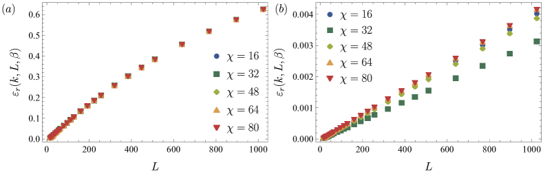
Figure 8: Scaling of the relative error $\varepsilon_{r}(k,L,\beta)$, defined in Eq. (49), as a function of the bond dimension $\chi$ used to approximate the thermal state. In the left panel we show data for the Ising chain while the right panel shows data for the XXZ chain. In both cases we use the same parameters as in Fig. 4. Data shown for $k=4$, other values of $k$ show similar behavior with $\chi=16$ being sufficient for convergence in the Ising model, while the XXZ model appears to be well converged from $\chi=64$.

First, we introduce the correlation lengths

$$e^{-\frac{1}{\zeta_{1}}}=\frac{{\rm max}_{j>0}\{|\lambda_{j}|\}}{\lambda_{0}}\,,\quad e^{-\frac{1}{\zeta_{2}}}=\frac{{\rm max}_{j>0}\{|\mu_{j}|\}}{\mu_{0}}\,,$$ (135)

and also

$$\zeta={\rm max}(\zeta_{1},\zeta_{2})\,.$$ (136)

Next, given the spectral decomposition in Eqs. (130), we define

$$C=\underset{\begin{subarray}{c}(j,k,l)\\ \neq(0,0,0)\end{subarray}}{{\rm max}}\left\{\frac{|\langle L_{j}^{(1)}|\langle L_{k}^{(1)}|R_{l}^{(2)}\rangle\langle L_{l}^{(2)}|R_{j}^{(1)}\rangle|R_{k}^{(1)}\rangle|}{|\langle L_{0}^{(1)}|\langle L_{0}^{(1)}|R_{0}^{(2)}\rangle\langle L_{0}^{(2)}|R_{0}^{(1)}\rangle|R_{0}^{(1)}\rangle|}\right\}\,.$$ (137)

Note that the denominator is non-vanishing because of Eqs. (132). We can now state the main result of this section.

Theorem 5.

Take $|I_{j}|=k$ with

$$k\geq k_{\rm min}={\rm max}\left\{1,\zeta\ln(20C\chi^{2}L)\right\}\,.$$ (138)

Then, for all

$$L\geq{\rm max}\{\zeta\ln(2^{5}\chi^{2}),4k+\zeta\ln(2\chi)\}\,,$$ (139)

we have

$$\left|\frac{r_{2}}{\mathcal{P}_{2}}-1\right|\leq\chi^{2}(80C+32)\frac{L}{k}e^{-k/\zeta}\,.$$ (140)

Proof.

Using Eqs. (130), we have

$$\mathcal{P}_{2}=\frac{\sum_{j=0}^{\chi^{2}-1}\mu_{j}^{L}}{\left(\sum_{j=0}^{\chi-1}\lambda_{j}^{L}\right)^{2}}=\frac{\mu_{0}^{L}}{\lambda_{0}^{2L}}\left(1+\tilde{\varepsilon}\right)\,,$$ (141)

where

$$\tilde{\varepsilon}=\frac{1+\sum_{j=1}^{\chi^{2}-1}(\mu_{j}/\mu_{0})^{L}}{\left(1+\sum_{j=1}^{\chi-1}(\lambda_{j}/\lambda_{0})^{L}\right)^{2}}-1\,.$$ (142)

Since by hypothesis $L\geq\zeta_{1}\ln(2\chi)$, we have $\chi e^{-L/\zeta_{1}}\leq 1/2$, and so

$$|\tilde{\varepsilon}| \leq 4\left(\chi^{2}e^{-L/\zeta_{2}}+2\chi e^{-L/\zeta_{1}}+\chi^{2}e^{-2L/\zeta_{1}}\right)$$

$$\leq 2^{4}\chi^{2}e^{-L/\zeta}\,.$$ (143)

On the other hand

$${\rm Tr}[\sigma_{I}^{2}]=\sum_{j,k=0}^{\chi-1}\lambda^{L-|I|}_{j}\lambda^{L-|I|}_{k}(\langle L_{j}^{(1)}|\otimes\langle L_{k}^{(1)}|)$$

$$\left(\sum_{l=0}^{\chi^{2}-1}\mu^{|I|}_{l}|R_{l}^{(2)}\rangle\langle L_{l}^{(2)}|\right)(|R_{j}^{(1)}\rangle\otimes|R_{k}^{(1)}\rangle)\,.$$ (144)

Therefore, recalling the definition (137), we have

$${\rm Tr} [\sigma_{I}^{2}]=\lambda_{0}^{2(L-|I|)}\mu_{0}^{|I|}\langle L_{0}^{(1)}|\langle L_{0}^{(1)}|R_{0}^{(2)}\rangle$$

$$\times\langle L_{0}^{(2)}|R_{0}^{(1)}\rangle|R_{0}^{(1)}\rangle\left(1+\varepsilon^{I}\right)\,,$$ (145)

where

$$|\varepsilon^{I}| \leq 2C\chi e^{-(L-|I|)/\zeta_{1}}+C\chi^{2}e^{-|I|/\zeta_{2}}$$

$$+ C\chi^{2}e^{-2(L-|I|)/\zeta_{1}}+2C\chi^{3}e^{-(L-|I|)/\zeta_{1}}e^{-|I|/\zeta_{2}}$$

$$+ C\chi^{4}e^{-2(L-|I|)/\zeta_{1}}e^{-|I|/\zeta_{2}}\,.$$ (146)

Since by hypothesis $L\geq 4k+\zeta\ln(2\chi)$, it is easy to verify that all the five terms above are upper bounded by $C\chi^{2}e^{-|I|/\zeta}$ (recall that $|I|\leq 2k$ for all $I$), and so

$$|\varepsilon^{I}| \leq 5C\chi^{2}e^{-|I|/\zeta}\leq 5C\chi^{2}e^{-k/\zeta}\,,$$ (147)

where we used that either $|I|=k$ or $|I|=2k$, and so $|I|\geq k$. Therefore

$$\frac{\prod_{j=1}^{R}{\rm Tr}_{I_{j}\cup I_{j+1}}(\sigma^{2}_{I_{j}\cup I_{j+1}})}{\prod_{j=1}^{R}{\rm Tr}_{I_{j}}\left[\sigma_{I_{j}}^{2}\right]}$$

$$=\frac{\mu_{0}^{L}}{\lambda_{0}^{2L}}\left(\frac{\prod_{j=1}^{R}(1+\varepsilon^{I_{j}\cup I_{j+1}})}{\prod_{j=1}^{R}(1+\varepsilon^{I_{j}})}\right)\,,$$ (148)

with $|\varepsilon^{I}|\leq 5C\chi^{2}e^{-k/\zeta}$. Combining this with Eq. (141), we arrive at

$$\frac{r_{2}}{\mathcal{P}_{2}}-1 =\left(\frac{\prod_{j=1}^{R}(1+\varepsilon^{I_{j}\cup I_{j+1}})}{\prod_{j=1}^{R}(1+\varepsilon^{I_{j}})}\right)\left(1+\tilde{\varepsilon}\right)^{-1}-1$$

$$= \left(1+\tilde{\varepsilon}\right)^{-1}\left[\frac{\prod_{j=1}^{R}(1+\varepsilon^{I_{j}\cup I_{j+1}})}{\prod_{j=1}^{R}(1+\varepsilon^{I_{j}})}-1-\tilde{\varepsilon}\right]\,,$$ (149)

where $\tilde{\varepsilon}$ is given in Eq. (142).

Next, we define

$$\varepsilon={\rm max}\left\{|\varepsilon^{I}|:I\in\{I_{j}\}_{j}\cup\{I_{j}\cup I_{j+1}\}_{j}\right\}\,.$$ (150)

By hypothesis $k\geq k_{\rm min}$ [$k_{\rm min}$ is given in (138)]. Therefore, using (147) we have $|\varepsilon^{I}|\leq 1/2$ for all $|I|$ and so also $\varepsilon\leq 1/2$. Therefore, we can apply the derivation in Lemma 1 to show

$$\left|\frac{\prod_{j=1}^{R}(1+\varepsilon^{I_{j}\cup I_{j+1}})}{\prod_{j=1}^{R}(1+\varepsilon^{I_{j}})}-1\right|\leq e^{(4L/k)\varepsilon}-1\,.$$ (151)

Since by hypothesis $L\geq\xi\ln(2^{5}\chi^{2})$, we also have $\tilde{\varepsilon}\leq 1/2$ [cf. Eq. (D)], and so (D) yields

$$\left|\frac{r_{2}}{\mathcal{P}_{2}}-1\right| \leq 2(e^{(4L/k)\varepsilon}-1)+2|\tilde{\varepsilon}|\,.$$ (152)

Finally, we note that Eq. (138) implies that $(4L/k)\varepsilon\leq 1$, and using $e^{z}-1\leq 2z$ for $0\leq z\leq 1$, we arrive at

$$\left|\frac{r_{2}}{\mathcal{P}_{2}}-1\right| \leq 80\chi^{2}C(L/k)e^{-k/\zeta}+2^{5}\chi^{2}e^{-L/\zeta}$$

$$\leq\chi^{2}(80C+32)\frac{L}{k}e^{-k/\zeta}\,.$$ (153)

∎

This theorem proves Eq. (45), under the condition (44). Therefore, the approximate factorization property (37) holds for MPDOs, with the identification

$$\alpha_{2}=(20C+8)\chi^{2}\,,\quad\beta_{2}=1/\zeta\,.$$ (154)

Appendix E Details on the numerical computations

In this Appendix we provide further details on the numerical computations performed to obtain the data presented in Secs. IV.4 and V. As mentioned, the calculations are carried out using the iTensor library Fishman et al. (2022), by first approximating the thermal states by MPOs of bond dimension $\chi$ and subsequently taking powers and traces of the density matrices represented in this way. For each quantity, we have always verified that the results were stable upon increasing the bond dimension $\chi$. An example of our data is reported in Fig. 8, where we study $\varepsilon_{r}(k,L,\beta)$, defined in Eq. (49), as a function of the bond dimension $\chi$ used to approximate the thermal state. In general, we have found that relatively small bond dimensions are enough in the quantum Ising chain, while larger bond dimensions are required in order to observe convergence in the Heseinberg model.

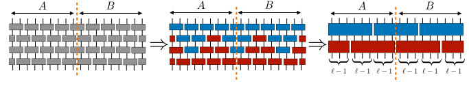
Figure 9: Any FDQC of depth $\ell$ can be rewritten as a depth-$2$ quantum circuit after grouping $\ell-1$ qubits into a single qudit. In the middle picture, we highlight with different colors sets of gates defining the two-qudit gates in the grouped lattice (colored rectangles in the right figure). In all the figures, a dashed orange line separates the regions $A$ and $B$, defining the bipartition of the system.

Appendix F Technical details on the PPT conditions

The goal of this Appendix is to identify the conditions under which the class of states $\rho^{(L)}(\gamma)$ introduced in Sec. V.2 satisfy Eqs. (56) for all system sizes $L$ and some suitable constants $C_{3}$, $C_{5}$ independent of $L$.

For concreteness, let the circuit depth $\ell$ be even, $\ell=2k$ with $k\geq 1$ (a similar discussion holds for $\ell=2k+1$) and take a bipartition of the system as in Fig. 9. We group neighboring sites into blocks containing $q=\ell-1$ qubits, forming a new super qudit associated with a Hilbert-space of dimension $d=2^{\ell-1}$. It is easy to show that the circuit can be rewritten as a depth-$2$ quantum circuit acting on the super qudits, cf. Fig. 9. Therefore (assuming without loss of generality $R=L/q$ is an integer)

$$\rho_{L}(\gamma)=V^{(2)}\left(\bigotimes_{j=1}^{L/q}\omega_{j}\right)\left[V^{(2)}\right]^{\dagger}\,,$$ (155)

where $\omega_{j}=\otimes_{i=1}^{q}\sigma_{jq+i}$, while

$$V^{(2)}=\left(\prod_{j}V_{2j,2j+1}\right)\left(\prod_{j}V_{2j+1,2j+2}\right)\,,$$ (156)

is the depth-$2$ FDQC acting on the super lattice.

As it is manifest from Fig. 9, the region $A$ contains all super qudits with labels from $1$ to $L/2q$, while $B$ contains all those with labels from $L/2q+1$ to $R=L/q$. Define the sets of super qudits $S_{1}=\{R/2-1,R/2\}$, $S_{2}=\{R/2+1,R/2+2\}$ and

$$\tilde{\rho}_{S_{1}S_{2}}=W\omega_{R/2-1}\otimes\omega_{R/2}\otimes\omega_{R/2+1}\otimes\omega_{R/2+2}W^{\dagger}\,,$$ (157)

where $W=V_{R/2,R/2+1}V_{R/2-1,R/2}V_{R/2+1,R/2+2}$. Note that $\tilde{\rho}_{S_{1}S_{2}}$ is different from the reduced density matrix over $S_{1}\cup S_{2}$. Using the graphical representation for the blocked circuits and Eq. (26), it is simple to show

$$\tilde{p}_{n}[AB]=\frac{{\rm Tr}\left[\left(\tilde{\rho}_{S_{1}S_{2}}^{T_{S_{1}}}\right)^{n}\right]}{{\rm Tr}_{S_{1}}[\tilde{\rho}_{S_{1}}^{n}]{\rm Tr}_{S_{2}}[\tilde{\rho}_{S_{2}}^{n}]}=:\tilde{s}_{n}\,,$$ (158)

where $\tilde{\rho}_{S_{1}}={\rm Tr}_{S_{2}}[\tilde{\rho}_{S_{1}S_{2}}]$ and $\tilde{\rho}_{S_{2}}={\rm Tr}_{S_{1}}[\tilde{\rho}_{S_{1}S_{2}}]$. Therefore, $\tilde{p}_{n}[AB]$ coincides with the normalized PT moments of the state $\tilde{\rho}_{S_{1}S_{2}}$, supported on four super qudits. Next, it is also easy to compute

$$\mathcal{P}_{n}[A] ={\rm Tr}_{S_{1}}[\tilde{\rho}^{n}_{S_{1}}][\gamma^{n}+(1-\gamma)^{n}]^{L/2-2q}\,,$$

$$\mathcal{P}_{n}[B] ={\rm Tr}_{S_{2}}[\tilde{\rho}^{n}_{S_{2}}][\gamma^{n}+(1-\gamma)^{n}]^{L/2-2q}\,.$$ (159)

Finally, setting

$$\tilde{t}_{3} =\frac{{\rm Tr}_{S_{1}}[\tilde{\rho}^{2}_{S_{1}}]^{2}{\rm Tr}_{S_{2}}[\tilde{\rho}^{2}_{S_{2}}]^{2}}{{\rm Tr}_{S_{1}}[\tilde{\rho}^{3}_{S_{1}}]{\rm Tr}_{S_{2}}[\tilde{\rho}^{3}_{S_{2}}]}\,,$$ (160)

$$\tilde{t}_{5} =\frac{{\rm Tr}_{S_{1}}[\tilde{\rho}^{4}_{S_{1}}]^{2}{\rm Tr}_{S_{2}}[\tilde{\rho}^{4}_{S_{2}}]^{2}}{{\rm Tr}_{S_{1}}[\tilde{\rho}^{3}_{S_{1}}]{\rm Tr}_{S_{2}}[\tilde{\rho}^{3}_{S_{2}}]{\rm Tr}_{S_{1}}[\tilde{\rho}^{5}_{S_{1}}]{\rm Tr}_{S_{2}}[\tilde{\rho}^{5}_{S_{2}}]}\,,$$ (161)

we arrive at

$$f_{3} =\tilde{s}_{3}-\tilde{s}_{2}^{2}\tilde{t}_{3}\frac{[\gamma^{2}+(1-\gamma)^{2}]^{2L-8q}}{[\gamma^{3}+(1-\gamma)^{3}]^{L-4q}}\,,$$ (162a)

$$f_{5} =\tilde{s}_{5}\tilde{s}_{3}-\tilde{s}_{4}^{2}\tilde{t}_{5}\frac{[\gamma^{4}+(1-\gamma)^{4}]^{2L-8q}}{[\gamma^{3}+(1-\gamma)^{3}]^{L-4q}[\gamma^{5}+(1-\gamma)^{5}]^{L-4q}}\,.$$ (162b)

Now, define

$$K_{3} ={\rm max}\{\tilde{s}_{3}(\gamma)-\tilde{s}^{2}_{2}(\gamma){\tilde{t}_{3}(\gamma)}:0\leq\gamma\leq 1/4\}\,,$$ (163)

$$K_{5} ={\rm max}\{\tilde{s}_{5}(\gamma)\tilde{s}_{3}(\gamma)-\tilde{s}^{2}_{4}(\gamma){\tilde{t}_{5}(\gamma)}:0\leq\gamma\leq 1/4\}\,,$$ (164)

and

$$H_{3} ={\rm max}\{|\tilde{s}^{2}_{2}(\gamma){\tilde{t}_{3}(\gamma)|}:0\leq\gamma\leq 1/4\}\,,$$ (165)

$$H_{5} ={\rm max}\{|\tilde{s}^{2}_{4}(\gamma){\tilde{t}_{5}(\gamma)|}:0\leq\gamma\leq 1/4\}\,.$$ (166)

The constants $K_{3}$, $K_{5}$, $H_{3}$, and $H_{5}$ depend on the specific choices of the unitary gates forming $U^{(\ell)}$. For non-entangling gates, $K_{3}$ and $K_{5}$ are positive, but for generic choices of gates one has $K_{3}<0$ and $K_{5}<0$. We are ready to state our main result.

Theorem 6.

Suppose $K_{3}$, $K_{5}<0$. Then, assuming without loss of generality $\gamma\leq 1/4$ and defining

$$C_{l}=\frac{|K_{l}|}{2}\,,\quad\gamma_{3}=-\frac{K_{3}}{4H_{3}},\quad\gamma_{5}=\left(-\frac{K_{5}}{8H_{5}}\right)^{1/3}\,,$$ (167)

we have

$$0\leq\gamma\leq\gamma_{3}/L\Rightarrow f_{3}\leq-C_{3}\,,$$ (168)

while

$$0\leq\gamma\leq\gamma_{5}/L^{1/3}\Rightarrow f_{5}\leq-C_{5}\,,$$ (169)

for all system sizes $L$.

Proof.

We start from Eq. (162a) and note

$$\frac{[\gamma^{2}+(1-\gamma)^{2}]^{2}}{\gamma^{3}+(1-\gamma)^{3}}=1-\varepsilon_{3}\,,$$ (170)

with $0\leq\varepsilon_{3}\leq\gamma$ for $0\leq\gamma\leq 1/4$. Therefore

$$f_{3} \leq K_{3}+\tilde{s}_{2}^{2}\tilde{t}_{3}[1-(1-\varepsilon_{3})^{L-4q}]$$

$$\leq K_{3}+H_{3}[1-(1-\gamma)^{L-4q}]\,.$$ (171)

Using $1-\gamma\geq e^{-2\gamma}$ for $0\leq\gamma\leq 1/4$, we get

$$f_{3} \leq K_{3}+H_{3}[1-e^{-2\gamma(L-4q)}]$$

$$\leq K_{3}+2H_{3}\gamma L\,.$$ (172)

Hence, if $\gamma\leq\gamma_{3}/L$, we finally arrive at

$$f_{3}\leq K_{3}/2=-C_{3}\,.$$ (173)

Analogously, we have

$$\frac{[\gamma^{4}+(1-\gamma)^{4}]^{2}}{[\gamma^{3}+(1-\gamma)^{3}][\gamma^{5}+(1-\gamma)^{5}]}=1-\varepsilon_{5}\,,$$ (174)

with $0\leq\varepsilon_{3}\leq 2\gamma^{3}$ for $0\leq\gamma\leq 1/4$. Therefore

$$f_{5} \leq K_{5}+\tilde{s}_{4}^{2}\tilde{t}_{5}[1-(1-\varepsilon_{5})^{L-4q}]$$

$$\leq K_{3}+H_{5}[1-(1-2\gamma^{3})^{L-4q}]\,.$$ (175)

Using $1-x\geq e^{-2x}$ for $0\leq x\leq 1/4$, we get

$$f_{5} \leq K_{5}+H_{5}[1-e^{-4\gamma^{3}(L-4q)}]$$

$$\leq K_{5}+4H_{5}\gamma^{3}L\,.$$ (176)

Hence, if $\gamma\leq\gamma_{5}/L^{1/3}$, we arrive at

$$f_{5}\leq K_{5}/2=-C_{5}\,.$$ (177)

∎

References

- Blatt and Roos (2012) R. Blatt and C. F. Roos, Nature Phys. 8, 277 (2012).
- Gross and Bloch (2017) C. Gross and I. Bloch, Science 357, 995 (2017).
- Schäfer et al. (2020) F. Schäfer, T. Fukuhara, S. Sugawa, Y. Takasu, and Y. Takahashi, Nature Rev. Phys. 2, 411 (2020).
- Kjaergaard et al. (2020) M. Kjaergaard, M. E. Schwartz, J. Braumüller, P. Krantz, J. I.-J. Wang, S. Gustavsson, and W. D. Oliver, Ann. Rev. Cond. Matt. Phys. 11, 369 (2020).
- Morgado and Whitlock (2021) M. Morgado and S. Whitlock, AVS Quantum Science 3, 023501 (2021).
- Monroe et al. (2021) C. Monroe, W. C. Campbell, L.-M. Duan, Z.-X. Gong, A. V. Gorshkov, P. W. Hess, R. Islam, K. Kim, N. M. Linke, G. Pagano, P. Richerme, C. Senko, and N. Y. Yao, Rev. Mod. Phys. 93, 025001 (2021).
- Alexeev et al. (2021) Y. Alexeev, D. Bacon, K. R. Brown, R. Calderbank, L. D. Carr, F. T. Chong, B. DeMarco, D. Englund, E. Farhi, B. Fefferman, et al., PRX Quantum 2, 017001 (2021).
- Pelucchi et al. (2022) E. Pelucchi, G. Fagas, I. Aharonovich, D. Englund, E. Figueroa, Q. Gong, H. Hannes, J. Liu, C.-Y. Lu, N. Matsuda, et al., Nature Rev. Phys. 4, 194 (2022).
- Burkard et al. (2023) G. Burkard, T. D. Ladd, A. Pan, J. M. Nichol, and J. R. Petta, Rev. Mod. Phys. 95, 025003 (2023).
- Preskill (2018) J. Preskill, Quantum 2, 79 (2018).
- Altman et al. (2021) E. Altman, K. R. Brown, G. Carleo, L. D. Carr, E. Demler, C. Chin, B. DeMarco, S. E. Economou, M. A. Eriksson, K.-M. C. Fu, et al., PRX Quantum 2, 017003 (2021).
- Elben et al. (2023) A. Elben, S. T. Flammia, H.-Y. Huang, R. Kueng, J. Preskill, B. Vermersch, and P. Zoller, Nature Rev. Phys. 5, 9 (2023).
- Elben et al. (2019) A. Elben, B. Vermersch, C. F. Roos, and P. Zoller, Phys. Rev. A 99, 052323 (2019).
- Cieśliński et al. (2023) P. Cieśliński, S. Imai, J. Dziewior, O. Gühne, L. Knips, W. Laskowski, J. Meinecke, T. Paterek, and T. Vértesi, arxiv:2307.01251 (2023).
- Huang et al. (2020) H.-Y. Huang, R. Kueng, and J. Preskill, Nature Phys. 16, 1050 (2020).
- van Enk and Beenakker (2012) S. J. van Enk and C. W. J. Beenakker, Phys. Rev. Lett. 108, 110503 (2012).
- Elben et al. (2018) A. Elben, B. Vermersch, M. Dalmonte, J. I. Cirac, and P. Zoller, Phys. Rev. Lett. 120, 050406 (2018).
- Knips et al. (2020) L. Knips, J. Dziewior, W. Kłobus, W. Laskowski, T. Paterek, P. J. Shadbolt, H. Weinfurter, and J. D. Meinecke, npj Quantum Inf. 6, 51 (2020).
- Ketterer et al. (2019) A. Ketterer, N. Wyderka, and O. Gühne, Phys. Rev. Lett. 122, 120505 (2019).
- Horodecki et al. (2009) R. Horodecki, P. Horodecki, M. Horodecki, and K. Horodecki, Rev. Mod. Phys. 81, 865 (2009).
- Nielsen and Chuang (2010) M. A. Nielsen and I. L. Chuang, Quantum computation and quantum information (Cambridge university press, Cambridge, UK, 2010).
- Calabrese and Cardy (2009) P. Calabrese and J. Cardy, J. Phys. A: Math. Theor. 42, 504005 (2009).
- Eisert et al. (2010) J. Eisert, M. Cramer, and M. B. Plenio, Rev. Mod. Phys. 82, 277 (2010).
- Islam et al. (2015) R. Islam, R. Ma, P. M. Preiss, M. Eric Tai, A. Lukin, M. Rispoli, and M. Greiner, Nature 528, 77 (2015).
- Kaufman et al. (2016) A. M. Kaufman, M. E. Tai, A. Lukin, M. Rispoli, R. Schittko, P. M. Preiss, and M. Greiner, Science 353, 794 (2016).
- Linke et al. (2018) N. M. Linke, S. Johri, C. Figgatt, K. A. Landsman, A. Y. Matsuura, and C. Monroe, Phys. Rev. A 98, 052334 (2018).
- Moura Alves and Jaksch (2004) C. Moura Alves and D. Jaksch, Phys. Rev. Lett. 93, 110501 (2004).
- Cardy (2011) J. Cardy, Phys. Rev. Lett. 106, 150404 (2011).
- Daley et al. (2012) A. J. Daley, H. Pichler, J. Schachenmayer, and P. Zoller, Phys. Rev. Lett. 109, 020505 (2012).
- Abanin and Demler (2012) D. A. Abanin and E. Demler, Phys. Rev. Lett. 109, 020504 (2012).
- Brydges et al. (2019) T. Brydges, A. Elben, P. Jurcevic, B. Vermersch, C. Maier, B. P. Lanyon, P. Zoller, R. Blatt, and C. F. Roos, Science 364, 260 (2019).
- Satzinger et al. (2021) K. J. Satzinger, Y.-J. Liu, A. Smith, C. Knapp, M. Newman, C. Jones, Z. Chen, C. Quintana, X. Mi, A. Dunsworth, et al., Science 374, 1237–1241 (2021).
- Stricker et al. (2022) R. Stricker, M. Meth, L. Postler, C. Edmunds, C. Ferrie, R. Blatt, P. Schindler, T. Monz, R. Kueng, and M. Ringbauer, PRX Quantum 3, 040310 (2022).
- Zhu et al. (2022) D. Zhu, Z. P. Cian, C. Noel, A. Risinger, D. Biswas, L. Egan, Y. Zhu, A. M. Green, C. H. Alderete, N. H. Nguyen, et al., Nature Comm. 13 (2022).
- Hoke et al. (2023) J. C. Hoke, M. Ippoliti, E. Rosenberg, D. Abanin, R. Acharya, T. I. Andersen, M. Ansmann, F. Arute, K. Arya, A. Asfaw, et al., Nature 622, 481 (2023).
- Zhou et al. (2020) Y. Zhou, P. Zeng, and Z. Liu, Phys. Rev. Lett. 125, 200502 (2020).
- Elben et al. (2020a) A. Elben, R. Kueng, H.-Y. R. Huang, R. van Bijnen, C. Kokail, M. Dalmonte, P. Calabrese, B. Kraus, J. Preskill, P. Zoller, and B. Vermersch, Phys. Rev. Lett. 125, 200501 (2020a).
- Cerezo et al. (2021) M. Cerezo, A. Sone, J. L. Beckey, and P. J. Coles, Quantum Sci. Tech. 6, 035008 (2021).
- Yu et al. (2021a) M. Yu, D. Li, J. Wang, Y. Chu, P. Yang, M. Gong, N. Goldman, and J. Cai, Phys. Rev. Res. 3, 043122 (2021a).
- Rath et al. (2021a) A. Rath, C. Branciard, A. Minguzzi, and B. Vermersch, Phys. Rev. Lett. 127, 260501 (2021a).
- Vitale et al. (2023) V. Vitale, A. Rath, P. Jurcevic, A. Elben, C. Branciard, and B. Vermersch, arXiv:2307.16882 (2023).
- Flammia et al. (2012) S. T. Flammia, D. Gross, Y.-K. Liu, and J. Eisert, New J. Phys. 14, 095022 (2012).
- Haah et al. (2016) J. Haah, A. W. Harrow, Z. Ji, X. Wu, and N. Yu, in Proceedings of the forty-eighth annual ACM symposium on Theory of Computing (2016) pp. 913–925.
- O’Donnell and Wright (2016) R. O’Donnell and J. Wright, in Proceedings of the forty-eighth annual ACM symposium on Theory of Computing (2016) pp. 899–912.
- Paini and Kalev (2019) M. Paini and A. Kalev, arXiv:1910.10543 (2019).
- Hadfield (2021) C. Hadfield, arXiv:2105.12207 (2021).
- Huang et al. (2021) H.-Y. Huang, R. Kueng, and J. Preskill, Phys. Rev. Lett. 127, 030503 (2021).
- Hadfield et al. (2022) C. Hadfield, S. Bravyi, R. Raymond, and A. Mezzacapo, Comm. Math. Phys. 391, 951 (2022).
- Rath et al. (2021b) A. Rath, R. van Bijnen, A. Elben, P. Zoller, and B. Vermersch, Phys. Rev. Lett. 127 (2021b).
- Vermersch et al. (2023) B. Vermersch, A. Rath, B. Sundar, C. Branciard, J. Preskill, and A. Elben, arXiv:2304.12292 (2023).
- Yen et al. (2023) T.-C. Yen, A. Ganeshram, and A. F. Izmaylov, npj Quantum Inf. 9, 14 (2023).
- Arienzo et al. (2023) M. Arienzo, M. Heinrich, I. Roth, and M. Kliesch, Quantum Inf. Comput 23, 961 (2023).
- Akhtar et al. (2023) A. A. Akhtar, H.-Y. Hu, and Y.-Z. You, Quantum 7, 1026 (2023).
- Bertoni et al. (2022) C. Bertoni, J. Haferkamp, M. Hinsche, M. Ioannou, J. Eisert, and H. Pashayan, arXiv:2209.12924 (2022).
- Ippoliti et al. (2023) M. Ippoliti, Y. Li, T. Rakovszky, and V. Khemani, Phys. Rev. Lett. 130, 230403 (2023).
- Ippoliti (2023) M. Ippoliti, arXiv:2305.10723 (2023).
- García-Pérez et al. (2021) G. García-Pérez, M. A. Rossi, B. Sokolov, F. Tacchino, P. K. Barkoutsos, G. Mazzola, I. Tavernelli, and S. Maniscalco, PRX Quantum 2, 040342 (2021).
- Georgescu et al. (2014) I. M. Georgescu, S. Ashhab, and F. Nori, Rev. Mod. Phys. 86, 153 (2014).
- Tacchino et al. (2020) F. Tacchino, A. Chiesa, S. Carretta, and D. Gerace, Ad. Quantum Tech. 3, 1900052 (2020).
- Daley et al. (2022) A. J. Daley, I. Bloch, C. Kokail, S. Flannigan, N. Pearson, M. Troyer, and P. Zoller, Nature 607, 667 (2022).
- Perez-Garcia et al. (2007) D. Perez-Garcia, F. Verstraete, M. M. Wolf, and J. I. Cirac, Quantum Inf. Comput. 7, 401 (2007).
- Cirac et al. (2021) J. I. Cirac, D. Pérez-García, N. Schuch, and F. Verstraete, Rev. Mod. Phys. 93, 045003 (2021).
- Cramer et al. (2010) M. Cramer, M. B. Plenio, S. T. Flammia, R. Somma, D. Gross, S. D. Bartlett, O. Landon-Cardinal, D. Poulin, and Y.-K. Liu, Nature Comm. 1, 149 (2010).
- Lanyon et al. (2017) B. Lanyon, C. Maier, M. Holzäpfel, T. Baumgratz, C. Hempel, P. Jurcevic, I. Dhand, A. Buyskikh, A. Daley, M. Cramer, et al., Nature Phys. 13, 1158 (2017).
- Qin et al. (2023) Z. Qin, C. Jameson, Z. Gong, M. B. Wakin, and Z. Zhu, arXiv:2306.09432 (2023).
- Baumgratz et al. (2013a) T. Baumgratz, D. Gross, M. Cramer, and M. B. Plenio, Phys. Rev. Lett. 111, 020401 (2013a).
- Baumgratz et al. (2013b) T. Baumgratz, A. Nüßeler, M. Cramer, and M. B. Plenio, New J. Phys. 15, 125004 (2013b).
- Holzäpfel et al. (2018) M. Holzäpfel, M. Cramer, N. Datta, and M. B. Plenio, J. Math. Phys. 59, 042201 (2018).
- Lidiak et al. (2022) A. Lidiak, C. Jameson, Z. Qin, G. Tang, M. B. Wakin, Z. Zhu, and Z. Gong, arXiv:2207.06397 (2022).
- Kokail et al. (2021) C. Kokail, R. van Bijnen, A. Elben, B. Vermersch, and P. Zoller, Nature Phys. 17, 936 (2021).
- Joshi et al. (2023) M. K. Joshi, C. Kokail, R. van Bijnen, F. Kranzl, T. V. Zache, R. Blatt, C. F. Roos, and P. Zoller, arXiv:2306.00057 (2023).
- Anshu et al. (2021) A. Anshu, S. Arunachalam, T. Kuwahara, and M. Soleimanifar, Nature Phys. 17, 931 (2021).
- Anshu and Arunachalam (2023) A. Anshu and S. Arunachalam, arXiv:2305.20069 (2023).
- Rouzé and França (2021) C. Rouzé and D. S. França, arXiv:2107.03333 (2021).
- Onorati et al. (2023) E. Onorati, C. Rouzé, D. S. França, and J. D. Watson, arXiv:2301.12946 (2023).
- Gross et al. (2010) D. Gross, Y.-K. Liu, S. T. Flammia, S. Becker, and J. Eisert, Phys. Rev. Lett. 105, 150401 (2010).
- Montanaro (2017) A. Montanaro, arXiv:1707.04012 (2017).
- Kuzmin et al. (2023) S. S. Kuzmin, V. I. Mikhailova, I. V. Dyakonov, and S. S. Straupe, arXiv:2309.00397 (2023).
- Torlai et al. (2018) G. Torlai, G. Mazzola, J. Carrasquilla, M. Troyer, R. Melko, and G. Carleo, Nature Phys. 14, 447 (2018).
- Zhao et al. (2023) L. Zhao, N. Guo, M.-X. Luo, and P. Rebentrost, arXiv:2309.09235 (2023).
- Luitz et al. (2014) D. J. Luitz, N. Laflorencie, and F. Alet, J. Stat. Mech. 2014, P08007 (2014).
- Stéphan et al. (2009) J.-M. Stéphan, S. Furukawa, G. Misguich, and V. Pasquier, Phys. Rev. B 80, 184421 (2009).
- Stéphan et al. (2010) J.-M. Stéphan, G. Misguich, and V. Pasquier, Phys. Rev. B 82, 125455 (2010).
- Alcaraz and Rajabpour (2013) F. C. Alcaraz and M. A. Rajabpour, Phys. Rev. Lett. 111, 017201 (2013).
- Stéphan (2014) J.-M. Stéphan, Phys. Rev. B 90, 045424 (2014).
- Leone et al. (2022) L. Leone, S. F. E. Oliviero, and A. Hamma, Phys. Rev. Lett. 128, 050402 (2022).
- Oliviero et al. (2022) S. F. E. Oliviero, L. Leone, and A. Hamma, Phys. Rev. A 106, 042426 (2022).
- Haug and Piroli (2023a) T. Haug and L. Piroli, Phys. Rev. B 107, 035148 (2023a).
- Haug and Piroli (2023b) T. Haug and L. Piroli, Quantum 7, 1092 (2023b).
- Lami and Collura (2023) G. Lami and M. Collura, Phys. Rev. Lett. 131, 180401 (2023).
- Tarabunga et al. (2023) P. S. Tarabunga, E. Tirrito, T. Chanda, and M. Dalmonte, arXiv:2305.18541 (2023).
- Niroula et al. (2023) P. Niroula, C. D. White, Q. Wang, S. Johri, D. Zhu, C. Monroe, C. Noel, and M. J. Gullans, arXiv:2304.10481 (2023).
- Vidal and Werner (2002) G. Vidal and R. F. Werner, Phys. Rev. A 65, 032314 (2002).
- Plenio (2005) M. B. Plenio, Phys. Rev. Lett. 95, 090503 (2005).
- Carteret (2005) H. A. Carteret, Phys. Rev. Lett. 94, 040502 (2005).
- Gray et al. (2018) J. Gray, L. Banchi, A. Bayat, and S. Bose, Phys. Rev. Lett. 121, 150503 (2018).
- Carteret (2016) H. A. Carteret, arXiv:1605.08751 (2016).
- Neven et al. (2021) A. Neven, J. Carrasco, V. Vitale, C. Kokail, A. Elben, M. Dalmonte, P. Calabrese, P. Zoller, B. Vermersch, R. Kueng, et al., npj Quantum Inf. 7, 152 (2021).
- Yu et al. (2021b) X.-D. Yu, S. Imai, and O. Gühne, Phys. Rev. Lett. 127, 060504 (2021b).
- Carrasco et al. (2022) J. Carrasco, M. Votto, V. Vitale, C. Kokail, A. Neven, P. Zoller, B. Vermersch, and B. Kraus, arXiv:2212.10181 (2022).
- Piroli et al. (2021) L. Piroli, G. Styliaris, and J. I. Cirac, Phys. Rev. Lett. 127, 220503 (2021).
- Malz et al. (2023) D. Malz, G. Styliaris, Z.-Y. Wei, and J. I. Cirac, arXiv:2307.01696 (2023).
- Chen et al. (2010) X. Chen, Z.-C. Gu, and X.-G. Wen, Phys. Rev. B 82, 155138 (2010).
- Hastings (2013) M. B. Hastings, Phys. Rev. B 88, 165114 (2013).
- Zeng et al. (2015) B. Zeng, X. Chen, D.-L. Zhou, and X.-G. Wen, arXiv:1508.02595 (2015).
- Zeng and Wen (2015) B. Zeng and X.-G. Wen, Phys. Rev. B 91, 125121 (2015).
- Rath et al. (2023) A. Rath, V. Vitale, S. Murciano, M. Votto, J. Dubail, R. Kueng, C. Branciard, P. Calabrese, and B. Vermersch, PRX Quantum 4, 010318 (2023).
- Poulin and Hastings (2011) D. Poulin and M. B. Hastings, Phys. Rev. Lett. 106, 080403 (2011).
- Kato and Brandao (2019) K. Kato and F. G. Brandao, Comm. Math. Phys. 370, 117 (2019).
- Brandão and Kastoryano (2019) F. G. Brandão and M. J. Kastoryano, Comm. Math. Phys. 365, 1 (2019).
- Kim (2017) I. H. Kim, arXiv:1709.07828 (2017).
- Svetlichnyy et al. (2022) P. Svetlichnyy, S. Mittal, and T. Kennedy, arXiv:2211.06794 (2022).
- Svetlichnyy and Kennedy (2022) P. Svetlichnyy and T. Kennedy, J. Math. Phys. 63, 072201 (2022).
- Haag et al. (2023) D. Haag, F. Baccari, and G. Styliaris, PRX Quantum 4, 030330 (2023).
- Chen et al. (2020) C.-F. Chen, K. Kato, and F. G. Brandão, arXiv:2010.14682 (2020).
- Kim (2021a) I. H. Kim, Phys. Rev. X 11, 021039 (2021a).
- Kim (2021b) I. H. Kim, arXiv:2109.11688 (2021b).
- Kuwahara et al. (2020) T. Kuwahara, K. Kato, and F. G. S. L. Brandão, Phys. Rev. Lett. 124, 220601 (2020).
- Kuwahara et al. (2021) T. Kuwahara, A. M. Alhambra, and A. Anshu, Phys. Rev. X 11, 011047 (2021).
- Silvi et al. (2019) P. Silvi, F. Tschirsich, M. Gerster, J. Jünemann, D. Jaschke, M. Rizzi, and S. Montangero, SciPost Phys. Lect. Notes , 8 (2019).
- Audenaert (2007) K. M. Audenaert, J. Phys. A: Math. Theor. 40, 8127 (2007).
- Chen et al. (2017) Z. Chen, Z. Ma, I. Nikoufar, and S. Fei, Science China, Phys. Mech. Astr. 60, 020321 (2017).
- Nielsen (2000) M. A. Nielsen, Phys. Rev. A 61, 064301 (2000).
- Farrelly (2020) T. Farrelly, Quantum 4, 368 (2020).
- Piroli and Cirac (2020) L. Piroli and J. I. Cirac, Phys. Rev. Lett. 125, 190402 (2020).
- Cirac et al. (2017) J. I. Cirac, D. Perez-Garcia, N. Schuch, and F. Verstraete, Ann. Phys. 378, 100 (2017).
- Sachdev (1999) S. Sachdev, Quantum phase transitions, Vol. 12 (Cambridge University Press, Cambridge (UK), 1999).
- Korepin et al. (1997) V. E. Korepin, N. M. Bogoliubov, and A. G. Izergin, Quantum inverse scattering method and correlation functions, Vol. 3 (Cambridge University Press, Cambridge (UK), 1997).
- Verstraete and Cirac (2006) F. Verstraete and J. I. Cirac, Phys. Rev. B 73, 094423 (2006).
- Fishman et al. (2022) M. Fishman, S. R. White, and E. M. Stoudenmire, SciPost Phys. Codebases , 4 (2022).
- Elben et al. (2020b) A. Elben, B. Vermersch, R. van Bijnen, C. Kokail, T. Brydges, C. Maier, M. K. Joshi, R. Blatt, C. F. Roos, and P. Zoller, Phys. Rev. Lett. 124, 010504 (2020b).
- Quan et al. (2006) H. T. Quan, Z. Song, X. F. Liu, P. Zanardi, and C. P. Sun, Phys. Rev. Lett. 96, 140604 (2006).
- Rana (2013) S. Rana, Phys. Rev. A 87, 054301 (2013).