The optimal resolution level of a protein
is an emergent property of its structure and dynamics

Abstract

Molecular dynamics simulations provide a wealth of data whose in-depth analysis can be computationally demanding and, sometimes, even unnecessary. Dimensionality reduction techniques are thus routinely employed to simplify and improve the interpretation of trajectories focusing on specific subsets of the system’s atoms; a still open problem, in this context, is to determine the optimal resolution level of the molecule, i.e. the smallest number of atoms needed to preserve the largest information content from the full atomistic trajectory. Here, we introduce the protein optimal resolution identification method (PROPRE), an unsupervised approach built on information theory principles that determines the smallest number of atoms that need to be retained in order to attain a synthetic yet informative description of a protein. By applying the method to a protein dataset and two particular case studies, we show that this number is typically between $1.5$ and $2$ times the amount of residues in a protein; furthermore, the degree of structural variability of the system influences the optimal resolution level importantly, in that a broader range of large-scale conformations correlates with fewer retained sites. The PROPRE method is implemented in efficient and user-friendly python scripts, which are made available for download on a github repository.

I Introduction

The in silico investigation of proteins enables researchers to disclose a wealth of information and insights in their biological function that is complementary to what experiments can provide. In particular, the high level of detail that is inherent in a computer model of a protein is largely out of reach for state-of-the-art experimental methods. In contrast, the highest resolution achievable in a computer model is atomistic, that is, each atom of the molecule is explicitly accounted for in the description; this is the case irrespectively of the strategy employed to compute the interactions among particles, which can range from quantum mechanical methods Amaro and Mulholland (2018); WOS (2020) to classical force fields Huang et al. (2017); Tian et al. (2019). In any case, the outcome of a simulation is a sequence of configurations providing the instantaneous positions of the protein’s atoms one time step after the other.

This high level of accuracy is strictly necessary to enable the calculation of forces and, consequently, the determination of the system’s time evolution in the correct manner (at least as correct as possible compatibly with the model employed). It is often the case, however, that the analysis of the trajectory does not need to focus on each and all atoms. In general, for example, hydrogen atoms are excluded from the analysis unless specific processes take place that involve them explicitly, e.g. hydrogen bond formation. Similarly, water molecules and ion atoms are necessary in the course of the simulation to reproduce a realistic environment of the protein, but it is generally ignored in the subsequent analysis unless the latter focuses on the interaction between the solute and the solvent.

In most cases, the study of a molecular dynamics (MD) trajectory can return useful, intelligible information if one is capable of identifying a few collective variables Van Der Maaten et al. (2009); Tribello and Gasparotto (2019) that describe, in a parsimonious and interpretable manner, the behaviour of the system. It is thus of paramount importance to perform a dimensionality reduction (DR) that projects the high-dimensional configuration of the molecule onto a lower-dimensional space of few, possibly nonlinear effective coordinates.

At present, several DR methods have been developed Ceriotti et al. (2011); Sittel and Stock (2018); Tribello and Gasparotto (2019) that serve this purpose through different kinds of strategies. In general, however, these techniques do not provide an unsupervised recipe for determining the optimal size of the low-dimensional, effective coordinate space that it makes sense to consider to have a sufficiently descriptive picture of the system. This issue is tightly related to a more fundamental question, namely, is there an optimal subspace size in terms of which the system should be described? In fact, before attempting at the identification of the most parsimonious, interpretable low-dimensional representation of the system, one should consider whether a specific size of the latter exists, and whether this is a property of the method or of the system.

In recent years, a DR strategy that is gaining growing attention is the identification of optimal mappings Giulini et al. (2020); Menichetti et al. (2021); Mele et al. (2022); Noid (2023). A mapping is, in general, a linear transformation that takes an atomistic configuration in input and returns the coordinates of fewer effective sites; a prototypical example of mapping is the projection of the positions of all a protein’s atoms onto those of the amino acid centres of mass. Another mapping strategy – which is the one we will focus on in this work – is the decimation mapping, whereby only a subset of the molecule’s atoms is retained, while the rest is ignored; a pictorial representation of this mapping is provided in Fig. 1.

By inspecting the MD trajectory of a protein in terms of a subset of the molecule’s atoms, one can highlight selected features of the system; a trivial yet illustrative example of this is the difference between a picture where only the alpha carbons are kept, and one where all atoms of a specific domain are retained: in the first case one gets the jist of the whole molecule’s fluctuations at a coarse level of description, in the second case only a specific portion of the molecule, possibly a functionally crucial one, is inspected with the highest detail, while the rest is simply ignored.

A large body of work has been carried out in the past few years to investigate the properties of mappings and their relation with the features of the underlying system that can be highlighted through them Shell (2008); Rudzinski and Noid (2011); Foley and Shell (2015); Giulini et al. (2021); Foley et al. (2020); Kidder et al. (2021); Noid (2023). Most importantly, a key idea is gaining ground, that a relation exists between the low-resolution description employed to inspect a system and the amount and type of useful information that can emerge Giulini et al. (2020); Menichetti et al. (2021); Foley et al. (2020); Noid (2023).

In this context, a crucial question pertains the level of resolution, loosely defined as the fraction of atoms retained in the coarse representation. As anticipated, in fact, one can wonder whether an optimal resolution level exists, at which it is particularly sensible, appropriate, and useful to study a molecular dynamics trajectory; this corresponds, in practice, to figure out how many atoms it makes sense to preserve in a more simplified description of the system. This issue precedes the identification of the most informative mapping(s) Diggins IV et al. (2018); Giulini et al. (2020), that is, which atoms in particular one should select and look at.

In this work we address two intertwined, complementary questions: on the one hand, we aim at understanding if the optimal atom number in terms of which it is most useful to describe a macromolecule can be interpreted as an intrinsic property of the system itself, and identified as such; on the other hand, we want to establish which relationships exist between this optimal resolution level and other structural and dynamical features of the molecule. To this end, we developed an unsupervised procedure based on an information-theoretical approach, which allows one to define a notion of information content in a quantitative manner; this algorithm, dubbed protein optimal resolution identification method, or PROPRE for short, processes an MD trajectory of a protein (but in principle is applicable to any macromolecule) and returns the optimal number of atoms that one should retain to build a synthetic yet maximally informative low-resolution representation of the system.

For the sake of clarity, we stress here that PROPRE provides an answer to the question “what is the optimal number of sites to retain?”, but it does not deal with the issues “where to optimally place the sites?” and “how to model the interactions between them?”. A coarse-grained model of a protein, to be optimally constructed in an unsupervised way on the basis of the information extracted from a plain, all-atom MD trajectory, requires one to take three distinct and consecutive steps:

1. Resolution level. First, one has to identify the optimal level of resolution at which the system should be modelled, which can be synthetically encoded in the number of atoms $N_{opt}$ to keep out of the total system size; this step can rely on the information contained in a plain atomistic MD run.

2. Resolution distribution. Second, one should pinpoint which atoms should be kept; in fact, the resolution level $N_{opt}$ is not sufficient to build a specific model, and a dedicated method is required to find the most appropriate subset of atoms to be employed as coarse-grained sites.

3. Effective interactions. Third, once also the specific mapping has been identified, effective interactions among the sites have to be put in place; this step is the one that has been historically more thoroughly addressed, as the vast available library of coarse-grained models for (bio)molecules demonstrates Giulini et al. (2021).

Here, our attention is fully focused on the first of these three issues; nonetheless, in the conclusion section we will frame the results of this work in relation to the other two.

In the rest of the paper we illustrate the theoretical foundations of the PROPRE algorithm, its technical workflow, and its application to nontrivial case studies that showcase its usage and results. The method is implemented in an agile and user-friendly python script that is made freely available for download and usage in the repository https://github.com/potestiolab/propre.

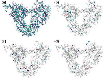
Figure 1: Example of different decimation mappings of a protein. Panel (a) shows a protein with $N_{ha}=2027$ heavy atoms. In panels (b), (c), and (d) $3$ different decimation mappings of the same protein are shown, selecting a subset of $N_{CG}=100$ atoms out of $N_{ha}$.

II The PROPRE method: theoretical background and algorithmic aspects

The PROPRE approach consists in a protocol for the analysis of an atomistic trajectory of a biomolecule, aimed at identifying the optimal number $N_{opt}$ of heavy atoms to build a synthetic yet informative description of the system. In other words, the method allows the determination of the optimal level of resolution to capture the essential features of the biomolecule’s dynamics, retaining the smallest amount of detail while preserving the largest amount of information.

In the following sections, the notions of amount of detail and amount of information will be made clearer and quantitative, and we will describe the theoretical foundations of PROPRE and its workflow. The software implementing the method, including the program itself and examples of input files, are freely available at the repository https://github.com/potestiolab/propre. The repository includes three python scripts: the first one removes all hydrogen atoms from both the molecule configuration file and the trajectory file; the second script computes the level of informativeness of various low-resolution representations as a function of the number of retained atoms, making use of two quantities, resolution and relevance, that are discussed in detail in the next subsection; the third script employs the results of the second to pinpoint the optimal number of sites; lastly, the script outputs plots of the processed data and files containing the relevant information. A more detailed description of the scripts usage and several examples of input files are available as readme files in the repository itself.

II.1 Resolution and relevance

The theoretical heart of PROPRE is the information extracted from the analysis of two quantities, namely resolution and relevance, computed on the data obtained from an MD simulation. The framework of resolution and relevance was originally developed by M. Marsili and coworkers Marsili et al. (2013); Cubero et al. (2019); Marsili and Roudi (2022), and found application for the analysis of data obtained in a number of different contexts, such as protein sequences Grigolon et al. (2016), neuron spike trains Cubero et al. (2020), and protein structure simulations Mele et al. (2022). The theoretical foundations of the method have been thoroughly presented and discussed in a rather large body of literature, towards which the interested reader is referred Marsili et al. (2013); Cubero et al. (2019); Marsili and Roudi (2022); Mele et al. (2022); Holtzman et al. (2022); here, we restrict ourselves to provide a definition of the quantities involved and the guidelines to their interpretation in the present context.

The starting point of our analysis is a collection of $M$ elements in a dataset. These elements can be of virtually any kind, e.g. strings of binary variables, images of real-valued pixels, or the spatial coordinates of a group of point-like particles. Without loss of generality, here we focus on the latter case, specifically the all-atom configurations sampled in the course of the MD simulation of a protein; each configuration thus represents an element of the collection.

These elements possess attributes that allow one to group them according to some criterion: for example, binary strings can be grouped according to the values of the first half of their bits; our protein configurations, on the other hand, can be clustered on the basis of their (dis)similarity: given a measure of distance between configuration pairs, different frames can be treated as the same if their distance is lower than a prescribed threshold. One of the many clustering methods on the market can thus serve as a tool to partition our configuration dataset in groups, each one containing elements that are identical according to the established criterion. A given grouping, or clustering, provides a “low-resolution” representation of the dataset, in that the differences among very similar elements are blurred away; out of $M$ elements (in principle all different from one another) we now have $L<M$ groups that describe the dataset in a less detailed manner.

A key idea of the resolution-relevance framework is that different levels of “blurring” are associated to different levels of information content, in a non necessarily intuitive manner. In fact, one might think that a high-resolution description of the dataset, all elements of which can be distinguished, contains a great deal of information; on the contrary, in absence of further information, all elements are just configurational singletons whose occurrence probability in the dataset is $1/M$. By clustering these elements, we indeed lose detail, but we acquire information in terms of the statistical weight of the clusters. Of course, a coarsening excess can be detrimental: if the elements are partitioned in one or few groups, very little detail remains in such a description to grasp any idea about the dataset and the information it contains. We have thus built the intuition that a low-resolution picture of our system can be more useful than a higher-resolution one, however an optimal trade-off point should be found to balance the amount of detailed lost and the amount of information gained.

This intuition, however, has to be made quantitative in order to be of practical use. To this end, we have to define adequate ways to measure the resolution level of a given dataset clustering and the amount of relevant information that such clustering contains.

Given our dataset of $M$ elements – in our case, the MD frames – we cluster them according to a measure of distance and a threshold. Such clustering thus produces a number of groups, to each of which we attribute a distinct label $s$. The resolution of this clustering is defined as its entropy $H_{res}$:

$$H_{res}[s]:=-\sum_{s}p_{s}\cdot\log_{2}(p_{s})$$ (1)

$$p_{s}:=\dfrac{k_{s}}{M}$$

where $k_{s}$ represents the count of dataset elements assigned to the cluster labelled by $s$. It is proven Cubero et al. (2019) that $H_{res}$ exhibits a continuous growth with an increasing number of clusters; this is consistent with the idea that the fewer the clusters, the lower the detail of our dataset representation, which is quantified by $H_{res}$. More specifically, the resolution is zero when all elements are gathered into the same group, since the probability for this unique cluster is $p_{s}=1$; in contrast, when each element is a singleton we have that $p_{s}=1/M\ \forall\ s$, and we have the largest value of resolution, $H_{res}=\ln M$.

As anticipated, it is also true, though, that a very detailed labelling that allows us to distinguish each dataset element from the other is not really useful. In fact, in absence of prior knowledge, each element is just as informative as any other, and no statistics – but the trivial, uniform one – is available to infer or reconstruct the generative process underlying the sample. If, on the other hand, we cluster elements, we gain insight in that different clusters are, in general, differently populated, and their relative size is a proxy for the statistical weight of the dataset elements they contain. Losing detail thus allows structure and information to emerge.

This qualitative picture is made quantitative by the relevance $H_{rel}$, which is defined as Marsili et al. (2013); Marsili and Roudi (2022):

$$H_{rel}[k]:=-\sum_{k}\dfrac{k\cdot m_{k}}{M}\cdot\log_{2}\left(\dfrac{k\cdot m_{k}}{M}\right)$$ (2)

where $m_{k}$ denotes the number of clusters containing the same amount $k=0,\dots,M$ of data points, for a given clustering process.

As it turns out, the relevance vs. resolution curve is bell-shaped. This is a consequence of the fact that the relevance, which is an entropy, is positive defined, and it is zero for both extreme values of the resolution. In fact, the case $H_{res}=0$ implies $m_{k}=1$ for $k=M$ and $m_{k}=0$ for all other values of $k$, which corresponds to $H_{rel}=0$. On the other hand, in the case where $H_{res}$ is the largest, one has $M$ clusters with one single element each, which corresponds to $m_{1}=M$ and every other $m_{k}=0$: once again, a scenario that leads to $H_{rel}=0$. By Rolle’s theorem, somewhere in between the extremes the curve $\left(H_{res},H_{rel}\right)$ has a maximum.

Normalising these quantities by $\ln M$, which is the largest value both of them can attain, they range between zero and unity, and while resolution grows from one extreme to the other, relevance goes from zero to a maximum and then back again to zero. A typical behaviour of this curve is reported in Fig. 3. A zero relevance at the extremes is a signal of the fact that having a perfectly detailed labelling, which allows one to tell each element apart from any other, is just as useless as a clustering that lumps all elements in a single “bucket”.

A special point in the plot is the one where the slope of the curve is $\mu=-1$ Marsili et al. (2013); Marsili and Roudi (2022); at this point, a loss of resolution by one unit is balanced by a gain in informativeness (as quantified by the relevance) of the same amount. For resolutions lower than that, the information gain is lower than the detail loss; this point is thus identified as the optimal compression point Marsili and Roudi (2022), where the resolution loss and the informativeness gain is optimally balanced.

A critical aspect of an analysis based on this framework is the fact that, in general, the resolution-relevance curve has the aforementioned bell shape irrespective of the dataset. This is to say that, whatever dataset we process, and whatever clustering strategy we employ, we will always get a curve of that type. This fact might lead one to erroneously assume either that any dataset entails some kind of information, or that the curves obtained through this method are meaningless, as even random data lead to that functional shape.

Key to the correct interpretation of these results is the fact that the resolution-relevance curve alone does not suffice. In fact, by reshuffling the content of the clusters while preserving their relative population keeps $H_{res}$ and $H_{rel}$ the same, as these quantities are agnostic to the elements themselves, and only depend on the cluster size. The physical significance of the curve strongly depends on the clustering procedure, which, in contrast, is informed of the properties of the dataset elements and groups them according to their characteristics. Once the clustering is performed, the resolution-relevance analysis serves to extract statistical information on the partitions, and in particular to assess the effectiveness of one partition relative to the others. This analysis thus provides information about the optimal, most informative level of dataset coarsening given the particular dataset at hand and the specific clustering strategy employed.

This state of things has been extensively investigated by some of us in a previous work Mele et al. (2022). There, we focused on the dependence of the resolution-relevance analysis on the specific procedure employed to cluster protein configurations. It was shown that this framework is indeed effective to optimally coarsen the conformational space of a protein, but the physical interpretability and soundness of the result largely rely on the clustering method. Certain methods are better at clustering than others, and this approach was proven capable of making this fact manifest.

In what follows, we will employ the resolution-relevance framework to pinpoint the optimal number of atoms to employ in a low-resolution representation of a protein structure; this number will be identified as that particular atom subset size such that, by operating a clustering based on the configurations of this subgroup alone, we obtain partitions entailing the largest amount of information about the behaviour of the molecule in the sample while, at the same time, reducing as much as possible the level of detail.

II.2 Calculation of the resolution-relevance curves

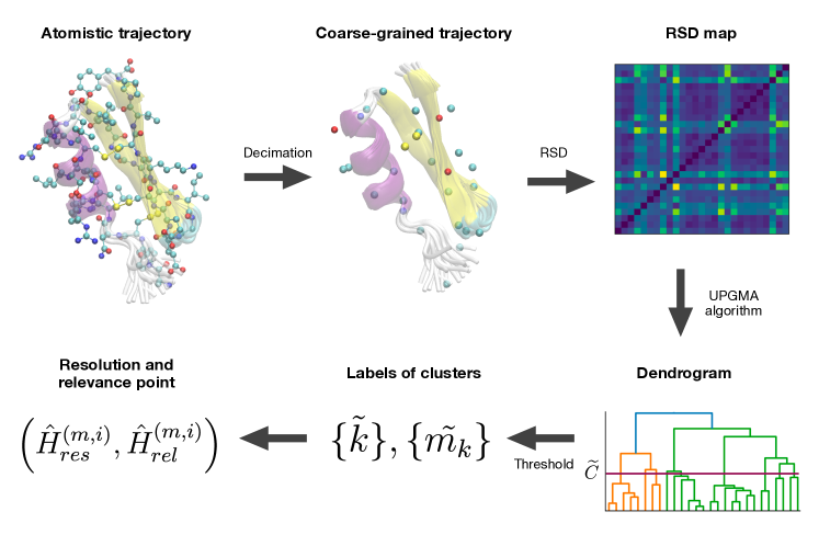
Figure 2: Infographic that illustrates the steps of the first part of the PROPRE protocol: the construction of the $H_{res},H_{rel}$ scatter plot. After filtering the atomistic trajectory (by choosing a random decimation mapping of the heavy atoms), the RSD map is built, in order to perform a clustering of the filtered configurations. Each mapping corresponds to a point in the $H_{res},H_{rel}$ plane; by varying the retained atoms selection as well as the number of retained atoms one can reconstruct the curve as a scatter plot.

The objective of this part of the workflow is to scan a range of numbers of retained (heavy) atoms and compute, for each of them, the values of resolution and relevance over a sample of randomly generated mappings. In this manner, we can construct a resolution-relevance curve in which the optimal resolution value, associated to the point of slope $-1$, can be identified. A schematic illustration of the whole workflow is provided in Fig. 2.

As anticipated, the starting point of the PROPRE algorithm is the molecular dynamics trajectory of a biomolecule, containing all atoms of the system of interest but not those of the solvent. Denoting with $N_{at}$ the number of heavy atoms in the molecule, the atomistic trajectory $\mathbf{X}_{ha}(t)$ consists in a collection of $T$ vectors of dimension $3N_{at}$, each labeled with the time index $t$ associated to the given time frame. In the applications presented here, this is the only a priori information we rely upon; in this way, we do not need to provide system- or case-specific details, but rather employ very basic data so as to avoid compromising the generality and the unsupervised nature of the method.

The UPGMA Sokal (1958) hierarchical clustering algorithm is then applied to cluster the configurations of $\mathbf{X}_{ha}(t)$. The metric employed to measure the distance between two configurations $\mathbf{X}^{a}$ and $\mathbf{X}^{b}$ is the root squared distance (RSD), defined as:

$$RSD=\sqrt{\sum_{i=1}^{N}|\mathbf{X}_{i}^{a}-\mathbf{X}_{i}^{b}|^{2}}.$$ (3)

The RSD is proportional to the more common root mean squared distance, $RSD=\sqrt{N}\cdot RMSD$, which, despite known limitations when used as a metric, still represents the most reliable, interpretable, and commonly used measure to quantify the dissimilarity between two protein structures Kufareva and Abagyan (2012).

The choice of employing the RSD is motivated by certain advantages it entails in the present context Giulini et al. (2020); Holtzman et al. (2022). Specifically, if we employed the RMSD as a measure of distance between pairs of configurations we would have to set, for each value of $N_{CG}$, a specific threshold for the clustering; on the contrary, the usage of the RSD allows us to choose a single threshold that can be employed irrespective of the number of sites that are retained at each iteration step. The aforementioned RSD distance threshold $\tilde{C}$ is the minimal value of dissimilarity, that is, the distance below which two configurations can be considered to be structurally identical. To set this value, we perform a hierarchical clustering of the all-atom trajectory, and define $\tilde{C}$ as the largest value below which all frames are distinguishable, i.e. each frame is representative of a singleton cluster. The threshold $\tilde{C}$ is then employed in the next step of the workflow; here we consider a number $N^{(i)}_{CG}=N_{ha}-i$ of retained atoms for $i\in[2,N_{ha}]$. A number $\mathcal{N}_{M}$ of different mappings is generated, that is, a random selection of $N^{(i)}_{CG}$ heavy atoms out of the $N_{ha}$ available ones. For each of the $\mathcal{N}_{M}$ mappings, the trajectory $\mathbf{X}_{ha}(t)$ is processed to obtain the configuration $\mathbf{X}^{(m,i)}_{CG}(t)$ of the sole atoms that are included in the mapping, the index $m$ labelling the specific mapping and $i$ indicating the retained atom number $N^{(i)}_{CG}$. The frames of this trajectory are clustered with the UPGMA algorithm, and the dendrogram is cut at the threshold value $\tilde{C}$: in this way, we group together those configurations that would be considered indistinguishable according to the criterion previously employed to separate the all-atom trajectory configurations; complementarily, two low-resolution configurations are treated as distinguishable if also the all-atom frames they derive from would be deemed distinct.

The clusters so obtained are then used to calculate one $(H_{res},H_{rel})$ point, see Eqs. 1 and 2; this procedure is repeated for each choice of the number of retained atoms $N^{(i)}_{CG}$ and for each random mapping $m$ generated retaining $N^{(i)}_{CG}$ atoms. The resulting points draw a curve in the resolution-relevance plane as the one shown in Fig. 3 for the protein adenylate kinase.

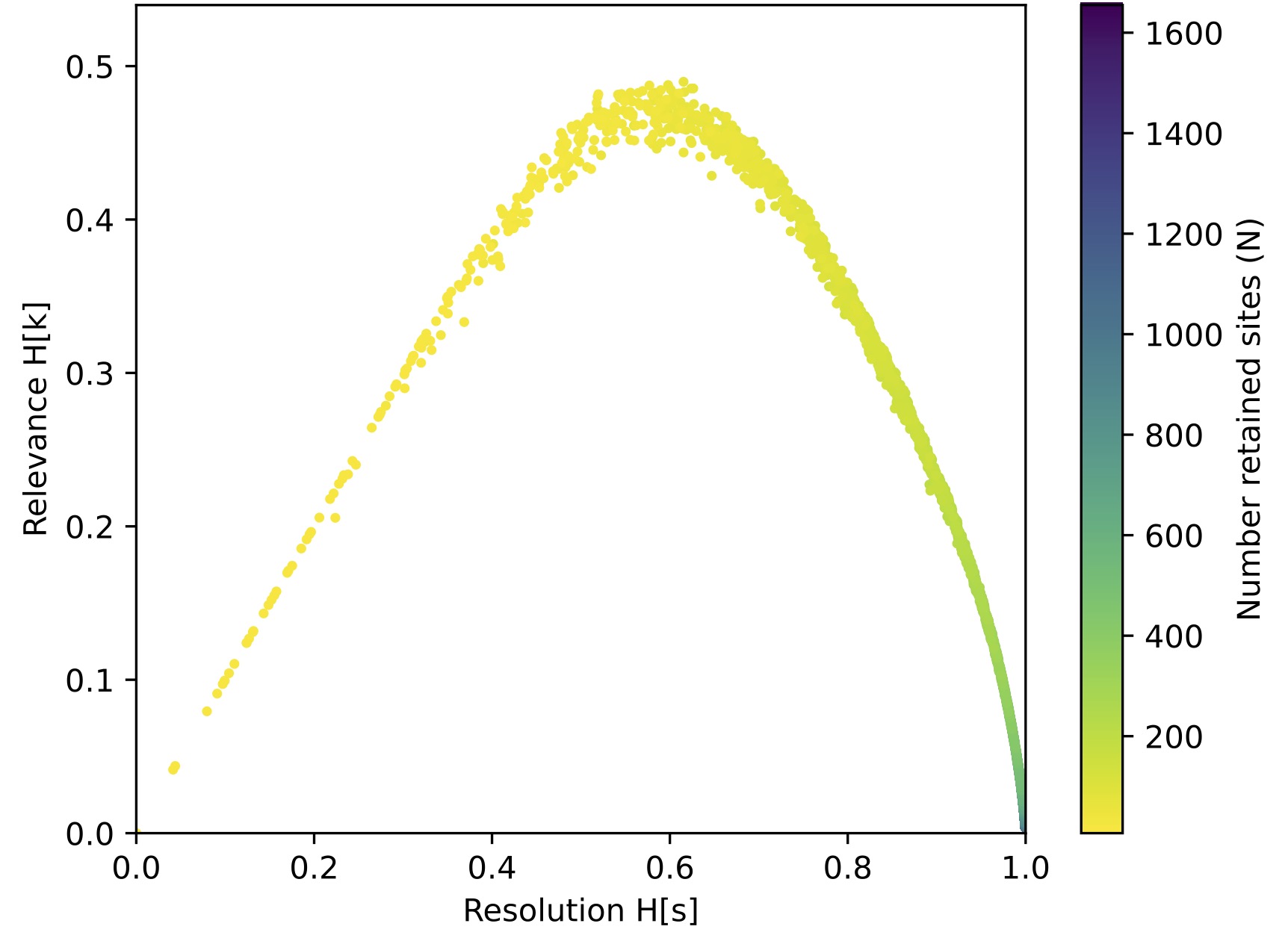
Figure 3: Plot of resolution ($H_{res}[s]$) vs. relevance ($H_{rel}[k]$) obtained for a trajectory of the enzyme adenylate kinase. Points are coloured according to the number of atoms retained in the corresponding mapping, transitioning from yellow to blue as the number increases.

II.3 Identification of the optimal number of retained sites

Once the relevance-resolution plot is constructed, the next step consists in identifying the point where the curve has slope $\mu=-1$, that is the point of optimal tradeoff between detail parsimony and information gain Marsili and Roudi (2022). This is a tricky step, in that we do not have a smooth, differentiable curve, but rather a scatter plot of points distributed on a range both in resolution and relevance.

In order to identify this soft spot, and find the number of retained atoms that best corresponds to it, one can proceed in at least two particularly intuitive ways: the uniform density and the uniform spacing averaging protocols. Each of the two consists in a rule to group the points that fall into the same, predefined resolution interval, and associate a single value of the relevance to each bin.

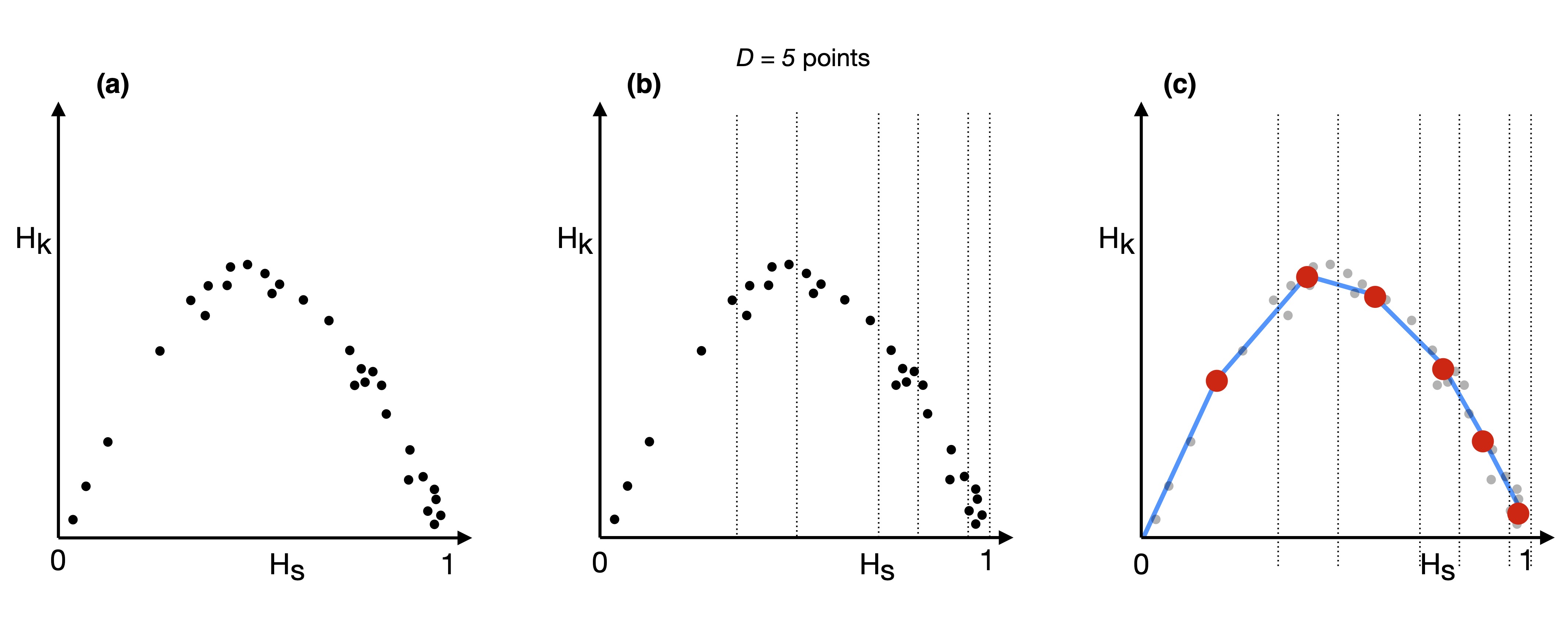
Figure 4: Uniform density approach to binning resolution-relevance curves. (a) pictorial representation of $30$ relevance and resolution points that we built ad hoc for a pictorial representation; (b) subdivision of the $x$ axis into intervals of variable width, each one containing $5$ points ($D=5$); (c) average curve of relevance and resolution (red circles and blue lines).

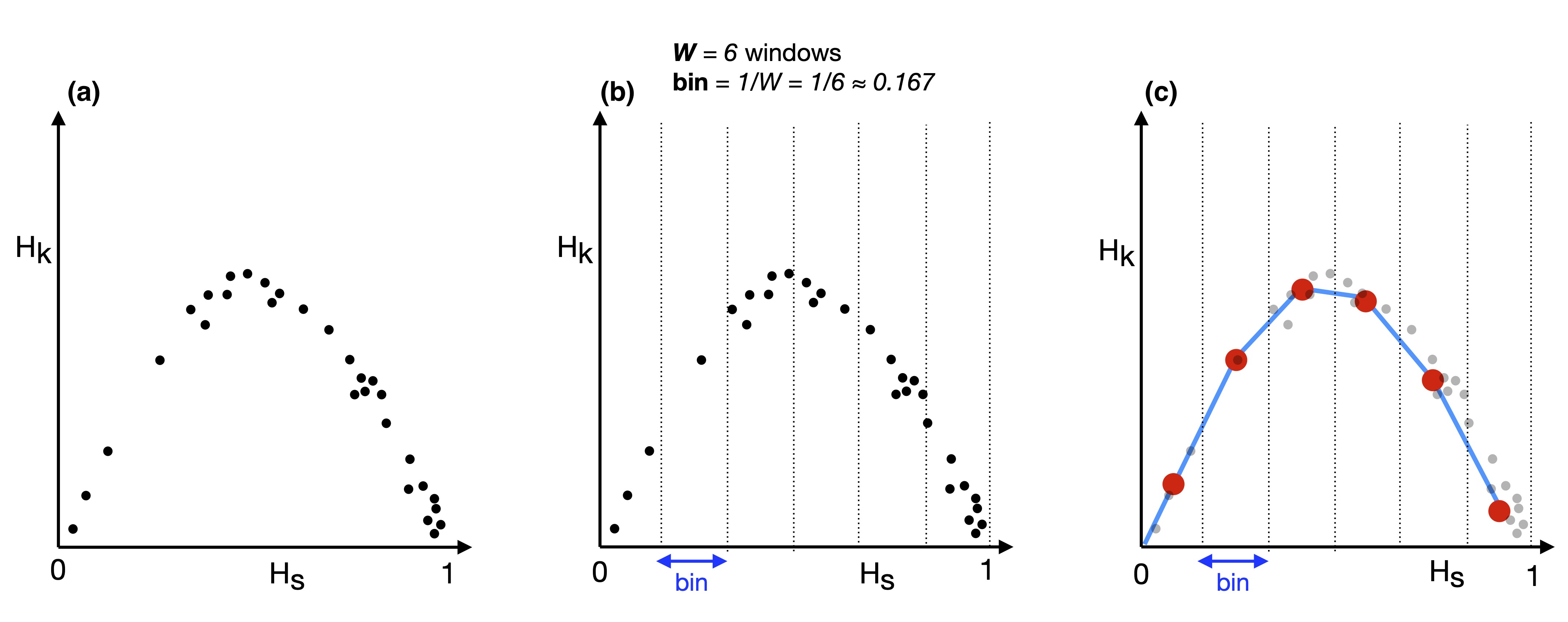
Figure 5: Uniform spacing approach to binning resolution-relevance curves. (a) pictorial representation of $30$ relevance and resolution points that we built ad hoc for a pictorial representation; b) subdivision of the $x$ axis into $6$ intervals of same length ($W=6$, bin width $1/W$), each one containing a variable number of points; (c) average curve of relevance and resolution (red circles and blue lines).

In the uniform density protocol, points are grouped so that every resolution interval contains the same number $D$ of $(H_{res},H_{rel})$ points: in this way, a uniform distribution of points is promoted by construction, and the value of the relevance, obtained averaging over the points in the bin, has a statistical weight comparable to that of the others. The default value of $D$ is set to $100$, but can be changed by the user. In Fig. 4 we illustrate the outcome of this procedure applied to a dataset of $30$ points that we built ad hoc for a pictorial representation; here, we chose to set the number of points per bin $D=5$ in order to have a sufficient number of both points and bins.

In contrast, in the uniform spacing protocol the $x$ axis is subdivided in $W$ intervals of width $1/W$, in order to promote a uniformly-distributed coverage of the resolution range. The default value of $W$ is $100$. Its application is illustrated in Fig. 5, where the number of windows has been set so as to have the same number of bins as in the previous case.

The choice of the method might depend on the specific necessity; in the applications explored in this work, the uniform density protocol is preferable as it returns a finer distribution of points in the region of interest to the PROPRE protocol, i.e. on the right of the maximum of $H_{res}$. We thus chose to implement this binning strategy in the algorithm, with a choice of $D=100$. The outcome of this smoothing procedure is a sequence of representative points, whose resolution value is given by the midpoint of the bins, and the relevance is given by the average of the points in the bin. Such representative points are indicated with red circles in Figs. 4 and 5.

Then, the program computes the numerical derivative of the curve of representative points. The method employed is the simple Newton’s difference quotient. Once the derivative is known, the algorithm highlights the points that correspond to a slope in the interval $[-1.1,-0.9]$ (as pictorially represented in Fig. 6(b)), a reasonable compromise between being accurately close to $-1$ and accounting for a function defined by a small and finite number of points. If more than one point falls into this region, the one with the highest resolution is kept. Finally, a histogram is built that counts the occurrence of a specific number of retained sites in the group of points belonging to the selected bin, see Fig. 6(b)c,d: the number with the highest occurrence is returned as the optimal number of retained heavy atoms $N_{opt}$.

The number of random mappings $\mathcal{N}_{m}$ that the program explores is very small compared to the number of possible selections of $N_{CG}$ atoms out of $N_{AT}>N_{CG}$ available ones. In fact, as it was discussed in depth in a previous work by some of us Menichetti et al. (2021), a complete, exhaustive coverage of the mapping space would be impossible in a time scale adequate to the practical needs we face here. However, the distribution of mappings at a given number of retained sites $N_{CG}$ is very narrow; this allows us to compute resolution and relevance on a relatively small number of mappings with the statistical guarantee that they will return a good estimate of the average.

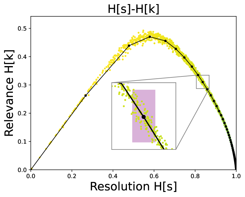
(a)

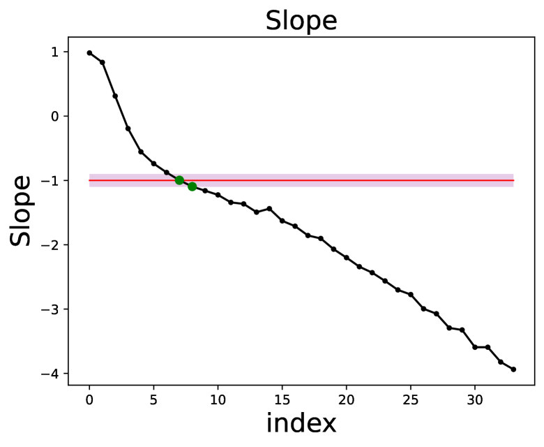
(b)

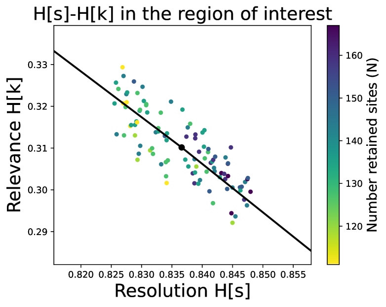
(c)

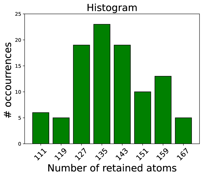
(d)

Figure 6: Summary output plots of the PROPRE workflow, applied to a 500 ns-long simulation of the adenylate kinase enzyme (discussed in detail in the Results section). (a) The production of the resolution-relevance scatter plot, with a zoom on the representative point identified by the slope $\tilde{\mu}\in[-1.1,-0.9]$. (b) Plot of the numerical slope $\tilde{\mu}$ as a function of the point index, highlighting in red the region $[-1.1,-0.9]$; here, two points are identified that fall in the highlighted region, however the approach outputs only the one corresponding to the largest number of occurrences, see panel (d). (c) Zoom on the points belonging to the bin highlighted in pink in (a). (d) Histogram of the occurrence of the various numbers of retained sites $N^{(i)}_{CG}$ in this bin; the output of the algorithm, $N_{opt}$, is the value of retained atoms with the largest number of occurrences.

III Materials and methods

III.1 Protein selection

A dataset of 11 proteins distinct in size, structure and function was built starting from a larger dataset of 107 proteins, after clusterization based on their dynamics. The initial, large dataset was based on the one employed in reference Hensen et al. (2012), from which proteins with too high sequence/structure similarity were removed. The proteins are categorized monomeric by the protein quaternary structure file server (PQS), have a resolution higher than 1.8Å, no ligands larger than six atoms, and no presence of metals other than Mg²⁺, Ca²⁺, K⁺, Na⁺, Zn⁺. Further requirements included a structure deposition date after 1987 and absence of gaps larger than one amino acid. The structures were downloaded from the Protein Data Bank, and the coordinate files were cleaned-up from heteroatoms, from copies of the protein in the crystallographic cell, and from residue-configurations with low occupancy. The position of missing atoms was rebuilt and the protein conformations were optimized using the software FoldXSchymkowitz et al. (2005). The procedure of dynamics-based clustering applied on this dataset reflects the one developed by us in Tarenzi et al. (2022), and already applied in Mele et al. (2022). Specifically, for each protein of the larger dataset, the first 10 normal modes of fluctuation were analysed using an elastic network model, and superimposed by means of the ALADYN protocol Potestio et al. (2010), which performs a hybrid structural/dynamical alignment. The similarity between the essential spaces spanned by the first 10 normal modes was quantified by means of the root mean square inner product (RMSIP) David and Jacobs (2011). The distance between the essential dynamics of two aligned proteins was defined as $d_{ij}=1-\textrm{RMSIP}_{ij}$; this distance was employed to perform a hierarchical clustering. The 11 proteins used in this work are the centroids of the resulting clusters, and their PDB codes are: 1DSL, 1NOA, 1SNO, 1UNE, 1XWL, 1IGD, 1HYP, 1KNT, 1QKE, 2EXO, 1KOE.

Two additional systems were employed to study the dependence of the optimal number of retained atoms on the protein conformational state, namely the enzyme adenylate kinase and the IgG4 therapeutic antibody pembrolizumab. These systems were chosen because of their large conformational variability, which can be sampled on timescales accessible to standard atomistic MD simulation. The starting structures for the MD simulations of these systems correspond to the crystallographic structure of ADK in the open form (PDB ID: 4AKE) and the full-length crystallographic structure of pembrolizumab (PDB ID: 5DK3). The residues missing from the antibody coordinate file were modelled as described in Tarenzi et al. (2021). The antibody has been simulated in two different conditions, namely in the presence and in the absence of the two glycans that are covalently bound to the Fc domain. To model the glycosylated pembrolizumab, the software doGlycans was employed Danne et al. (2017). Firstly, the glycans structures where defined by a sequence that comprises information on the type of sugar moieties and their connectivity; the employed glycans are composed by 4 N-acetylglucosamines, 3 mannoses, and 1 fucose (Glc-NAc4Man3Fuc). Secondly, the topology of the sugar is generated and it is included in the topology of the global system that contains all the parameters of the protein, the sugars, and the solvent. Residues N297 of both heavy chains were glycosylated, as reported in the work of Scapin et al. Scapin et al. (2015). The structure of the glycosylated antibody was visually checked, and torsional angles of the carbohydrates were adjusted to avoid steric clashes between the sugar chains as well as between the sugar and the protein atoms.

III.2 Simulation details

All simulations were performed with the Gromacs 2018 software Abraham et al. (2015). The protein topology was defined through the AMBER99SB-ILDN force field Lindorff-Larsen et al. (2010), and the TIP3P model was employed for the description of water molecules Jorgensen et al. (1983). Sodium and chloride ions were added at the physiological concentration of $150$ mM, neutralising the global electric charge in the simulation box. After energy minimisation, NVT and NPT equilibrations were performed using the velocity-rescale thermostat Bussi et al. (2007) and the Parrinello–Rahman barostat Parrinello and Rahman (1981). A cut-off of $1.2$ nm was used for van der Waals interaction and for the short-range component of the Coulomb one. The long-range component of the Coulomb force, instead, was computed with the Particle Mesh Ewald algorithm. The LINCS Hess et al. (1997) algorithm was employed to define the constraints on the hydrogen-containing bonds. An integration time step of $2$ fs was used. For each protein of the dataset, a trajectory of $500$ ns was collected; of these, the first $100$ ns are considered as equilibration and therefore discarded from the following analysis. Adenylate kinase was simulated for $500$ ns as well, while the antibody pembrolizumab was simulated for $2$ $\mu$s, in $4$ independent replicas of $500$ ns each. In the case of ADK and pembrolizumab, the trajectory frames were assigned to different conformational basins on the basis of the root-mean-square deviation between structures, as described in Fiorentini et al. (2023) for ADK and Tarenzi et al. (2021) for pembrolizumab.

III.3 PROPRE parameters

For each simulation, 1000 frames, equally spaced along the trajectory, are used for the PROPRE analysis. In accordance with the default software parameters, the number of random mappings for a fixed number of CG sites is $50$, while the number of retained atoms itself is progressively decreased with a step corresponding to $0.5$% of the total number of protein heavy atoms. From the computed relevance-resolution curves, the uniform density protocol is applied for smoothing, using a value of $100$ points per resolution bin.

III.4 Analysis

Analysis of the trajectories was performed with Gromacs tools and in-house scripts. Protein residue fluctuations were calculated with gmx rmsf, while the clustering and the identification of the representative conformations was performed with gmx cluster. The rendering of protein structures was performed with VMD Humphrey et al. (1996) and with TCL scripts.

IV Results and discussion

IV.1 Optimal number of sites vs number of protein residues

The PROPRE algorithm allows the identification of the optimal resolution for a specific protein, where the optimal resolution is intended as the fraction of the total number of sites (namely, of the protein heavy atoms) that has to be retained in order to minimize the information loss upon coarse-graining. It is natural to think that the optimal number of sites $N_{opt}$ depends on the specific system under investigation and its features, e.g. the protein size, architecture, and flexibility. To assess the possible presence of a general trend, we fist applied the PROPRE pipeline to $500$ ns-long MD trajectories of a set of $11$ different proteins (Fig. 7), ranging from a molecular weight of $7$ kDa (1IGD) to $66$ kDa (1XWL). The systems were selected from a larger protein dataset in order to maximize the differences in tertiary structure and dynamical features (see Methods section). Despite the large differences in structure, size and dynamics, the analysis on the trajectories of the 11 proteins of the dataset suggests a relation between the optimal number of retained sites and the total number of protein residues. The plot in Fig. 8 shows indeed a linear trend between these two quantities, with a correlation coefficient $R^{2}=0.81$. The slope of the curve is $1.82$, meaning that, in general, the optimal number of retained atoms is between $1.5$ and twice the number of protein residues.

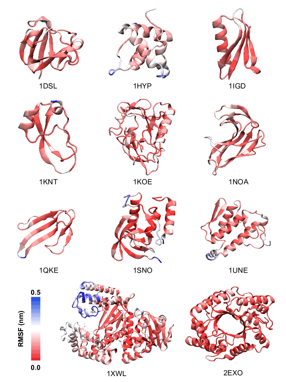
Figure 7: Graphical representation of the proteins comprising the dataset, colored according to the per-residue value of root-mean-square fluctuations as computed from the MD simulations.

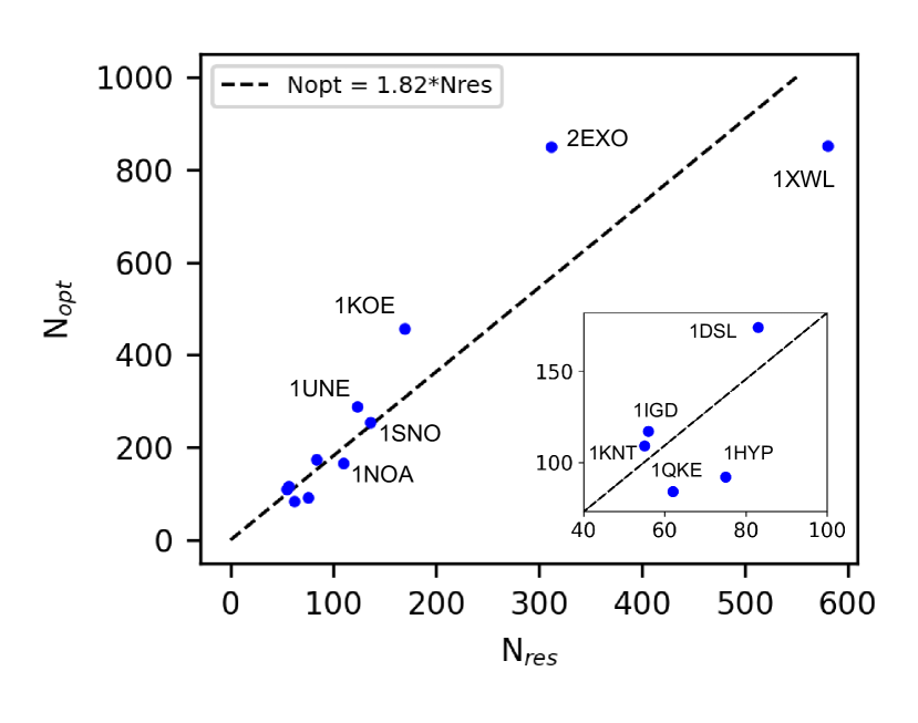
Figure 8: Scatter plot of the number of optimal sites identified by PROPRE for each protein of the dataset, in relation to the number of residues.

The general trend just discussed, however, is accompanied by nontrivial deviations observed in the case of the largest proteins of the dataset, namely 1KOE, 2EXO, and 1XWL. In fact, the first two have a larger optimal number of retained atoms than expected, while the third one turns out to be aptly described by fewer sites. A more detailed inspection of these cases shows that proteins 1KOE and 2EXO have a fairly stiff structure and a rather limited range of fluctuations, as it can be seen from the RMSD-based colouring in Fig. 7; in contrast, protein 1XWL is not only the largest of the dataset, but also a very mobile one. This suggests that the optimal fraction of retained atoms might be affected by other factors in addition to the protein size, such as the degree of flexibility and the diversity of conformational states explored during the MD simulation. To put this idea at test, in the following we discuss the case of two very flexible molecules, namely the enzyme adenylate kinase and the antibody pembrolizumab.

IV.2 Optimal number of sites vs protein conformational state

The enzyme adenylate kinase

To investigate the dependence of $N_{opt}$ on the conformations of the biomolecules, the PROPRE analysis has been performed on a $500$ ns-long simulation of the adenylate kinase (ADK) enzyme, sampling both the open and the partially closed states of the protein (Fig. 9). In the partially closed conformation, the distance between the LID and NMP domains is substantially reduced with respect to the open one. We do not observe a complete transition between the open and fully closed states, as expected from the absence of the substrate and from the long time scale of the process Zheng and Cui (2018); this partially closed conformation of ADK in the apo state was already observed both experimentally Henzler-Wildman et al. (2007) and in previous MD simulation studies Li et al. (2015); Wang et al. (2020) performed in similar conditions. On the basis of the different RMSD between the two conformational states, we grouped the all-atom frames from the full trajectory in two clusters, corresponding to the open and closed conformation; we then applied PROPRE to compute the optimal number of retained atoms on the full trajectory and on the two individual structural basins. The values of $N_{opt}$ in these three cases is plotted in Fig. 10 as a function of the mean square displacement (MSD) of the C_α atoms, averaged over the residues and the trajectory frames.

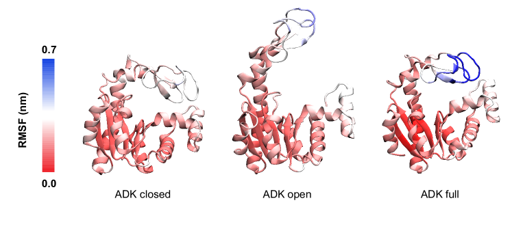
Figure 9: Representative structures of the ADK enzyme in the compact and open conformations, and representative structure of the protein as extracted from the full trajectory. Each structure is colored according to the per-residue value of root-mean-square fluctuations.

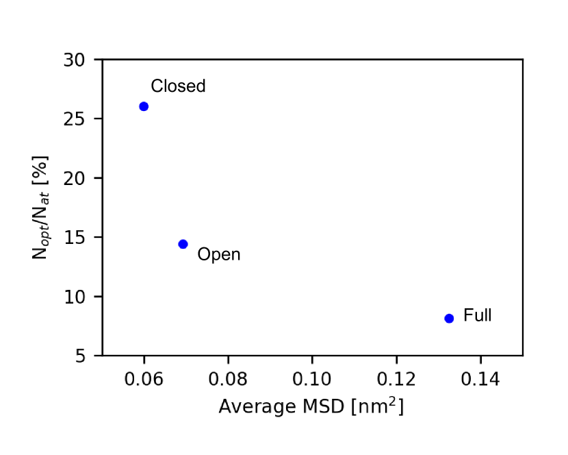
Figure 10: Scatter plot of the fraction of the number of optimal sites computed on the full ADK trajectory, and on the subsets of configurations obtained after clustering the simulation in the open and closed states, as a function of the mean square displacement within each trajectory.

The results show that each of the three cases corresponds to a different optimal number of retained atoms, although the system (and therefore the total number of protein atoms) is the same. In particular, $N_{opt}$ decreases with the occurrence of large-scale fluctuations along the simulation. In the case of the full trajectory, where large-scale transitions between the open and compact states are sampled and the MSD (averaged on the protein residues) is the largest, the fraction of retained atoms is only the $8$%; in the cluster of the open state, where the fluctuations are reduced but a good degree of flexibility is still present, the percentage is $14$%; and in the cluster of the compact state, where the conformation of the protein is such that all large-scale fluctuations are hindered, the percentage increases to $26$%. Incidentally, applying the criterion obtained in Section IV.1 for the calculation of $N_{opt}$ using only the number of residues as input, the resulting $N_{opt}/N_{at}$ value is $23.5$%, which is very close to the result obtained for the closed conformational cluster. Once again, this suggests that this criterion applies only to the cases of compact and rigid proteins, while the system-specific flexibility and configurational variability must be taken into account in more general cases.

The IgG4 antibody pembrolizumab

Antibodies are highly flexible molecules, and as such they represent a perfect test-case for the calculation of $N_{opt}$ in relation to the protein’s conformational state. We focused on the IgG4 antibody pembrolizumab, here investigated in two different forms: the non-glycosilated and the glycosilated ones. In both cases, the antibody is simulated in the apo form, without the presence of the antigen.

For both the non-glycosilated and the glycosilated states, four 500 ns-long simulations of the full-length antibody pembrolizumab were collected, and the resulting configurations clustered according to the protein conformation similarity. The resulting clusters are ordered according to the increasing average radius of gyration, and labelled from 0A to 5A for the non-glycosilated state (Fig. 11) and from 0G to 3G for the glycosilated state (Fig. 12). Calculations of the optimal number of sites were performed on each conformational cluster. The results for the non-glycosilated systems are plotted in Fig. 13.a. Also in this case, larger protein fluctuations lead to a lower percentage of retained atoms, although this trend is less well-defined for the low-MSD clusters. In contrast, this behaviour is particularly clear in the case of the antibody in the glycosilated state (Fig. 13.b), where there is an evident relation between the degree of flexibility within a conformational basin and the optimal number of representative sites.

It is worth noticing that the fraction of $N_{opt}$, as predicted following the rule of thumb in Section IV.1, amounts to the 23% of the total number of heavy atoms in the protein, a value almost double than those plotted in Fig. 13; this observation further corroborates the idea that the discrepancy between the two optimal fractions of retained atoms can be explained on the basis of the high flexibility of the protein structure, even within those conformational clusters displaying the lowest fluctuation intensities.

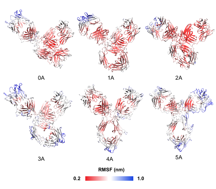
Figure 11: Representative structure of each conformational cluster obtained from the trajectories of the antibody pembrolizumab in the apo form, colored according to the per-residue value of root-mean-square fluctuations as computed from the MD simulations.

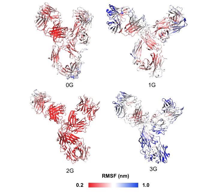
Figure 12: Representative structure of each conformational cluster obtained from the trajectories of the antibody pembrolizumab in the glycosilated form, colored according to the per-residue value of root-mean-square fluctuations as computed from the MD simulations.

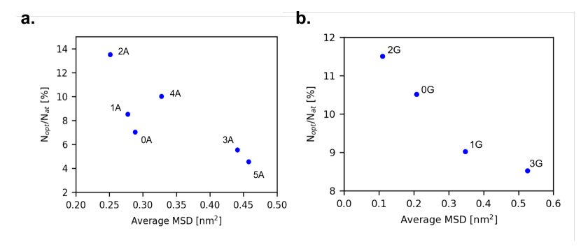
Figure 13: Scatter plot of the fraction of the number of optimal sites computed on each conformational cluster extracted from the non-glycosylated (a) and glycosylated (b) antibody trajectories, as a function of the average mean square displacement

within each cluster.

V Conclusions

The resolution at which one inspects a system is not a neutral or irrelevant parameter. Indeed, whatever the level of detail employed to model the system (quantum, classical, atomistic, coarse-grained…), the choice of how much of it to look at is in the hand of the observer; such choice is inevitable (we can’t process all $3N$ coordinates of a large molecule at once) and fraught with consequences, as it is any decision to keep something and discard something else.

The selection of what to preserve is subjected to the identification of the right amount of detail to keep, in our case being the number of heavy atoms of a protein that it makes sense to retain in order to have a sufficiently compact and yet informative picture of the molecule.

In this work we have illustrated an algorithmic, unsupervised strategy that, taking the moves from general concepts of information theory, allows one to process a molecular dynamics trajectory (or any other collection of configurations, irrespectively of their origin) and identify the optimal fraction of heavy atoms to employ in a coarse-grained description of the system. The resulting optimal number of atoms to keep turns out to range between $1.5$ and $2$ times the number of amino acids of the protein (or of alpha carbons, equivalently), suggesting that typical one-bead-per-amino acid coarse-grained models might be at risk of missing important structural and dynamical features unless these are not adequately encoded in the effective interaction potentials Giulini et al. (2020); Noid (2023). Furthermore, the optimal number of retained atoms is found to have a strong dependence on the structural variability of the conformational basin explored in the course of the simulation. More specifically, a broader range of distinct configurations explored correlates with a lower optimal number of retained atoms, and vice versa; this is suggestive of the fact that a small number of reference atoms suffices to grasp the structural variability of a molecule that “breathes a lot”, while many more atoms are needed to distinguish, with the same level of resolution, configurations that differ by small, quasi-random fluctuations. This result is in full agreement with the well-known notion that only large-scale, highly collective motions can be appropriately described in terms of a small number of collective variables Yang et al. (2007), a notion broadly supported by results obtained from established dimensionality reduction techniques such as principal component analysis David and Jacobs (2014) and normal mode analysis Bauer et al. (2019).

The picture that emerges thus suggests that, for a given sample of conformations of a protein, it is possible to identify a specific level of detail at which the system under examination can be most appropriately described; at this resolution level, the largest amount of information can be extracted in terms of the smallest amount of data. Furthermore, this optimal coarsening is an intrinsic property of the configuration dataset, as it can be identified on the sole basis of the latter, in absence of additional, complementary information. This property thus emerges from the features of the sample, and it can be interpreted in the light of the system structure and dynamics in a simple and intelligible manner.

The approach presented here is general and easy to employ; the outcome of its application to a sample of conformations of a protein does not only consist in a number of atoms to retain, but rather in a quantitative assessment of the amount of informative detail that one can extract out of this sample. In particular in the context of multiscale modelling, the identification of the smallest number of atoms that return a minimal yet informative picture of the molecule can serve a dual purpose. On the one hand, it can be used for an a posteriori analysis, which enables one to gain insights into the dynamic behavior of the molecule within the trajectory itself. The optimal atom subset allows an in-depth inspection of the system without having to account for all its degrees of freedom, thereby preserving key but subtle details while making their quantitative study easier and computationally lighter. The same trajectory can be investigated in function of its length, of the conformational basins it explores, and the biological state of the molecule. The efficient workflow of PROPRE is thus ideally suited for large-scale, dataset-wide analyses.

On the other hand, a complementary usage of the PROPRE method is the construction of a coarse-grained/multiscale model. In the introduction we mentioned that this objective entails three distinct steps: the assessment of the appropriate resolution level; the identification of the specific sites to model the system at the selected low resolution; and the parametrisation of the effective interactions among these sites. In previous works, some of us have addressed the second and the third steps: in particular, a method was developed, the mapping entropy optimisation workflow, that identifies which atoms of the protein are especially important to preserve in a coarser model Giulini et al. (2020); Holtzman et al. (2022), and an efficient, algorithmic strategy was proposed, the coarse-grained anisotropic network model for variable resolution simulations Fiorentini et al. (2023), or CANVAS for short, by which one can build the effective interactions for a multiple-resolution protein model, i.e. one whose coarse-grained resolution is not uniform.

The PROPRE algorithm completes the aforementioned pipeline by providing a strategy to set, in an unsupervised manner, the number of sites that the model should entail; with the introduction of PROPRE, we thus make a self-contained, practical and efficient instrument for protein analysis and multi-scale modelling available to the community.

In conclusion, the PROPRE approach represents a useful tool to shed new light on otherwise rather hidden features of a protein, helping researchers to build a quantitative, direct path between the properties of the system and the way one looks at it.

VI Acknowledgments

The authors are indebted with R. Menichetti and L. Tubiana for an insightful reading of the manuscript and useful comments. RP acknowledges support from the Italian Ministry of Education, University and Research (MIUR) through the FARE grant for the project HAMMOCK (grant R18ZHWY3NC). RP acknowledges support from ICSC - Centro Nazionale di Ricerca in HPC, Big Data and Quantum Computing, funded by the European Union under NextGenerationEU. Views and opinions expressed are however those of the author(s) only and do not necessarily reflect those of the European Union or The European Research Executive Agency. Neither the European Union nor the granting authority can be held responsible for them.

VII Author contributions

RP conceived the study and proposed the method. RF and GM wrote the software. RF and TT ran the MD simulations and performed the analysis. All authors contributed to the analysis and interpretation of the data. All authors drafted the paper, reviewed the results, and approved the final version of the manuscript.

VIII Data availability

The raw data associated with this work are freely available on github at https://github.com/potestiolab/propre and on the MaterialsCloud Archive at https://doi.org/10.24435/materialscloud:a7-r8.

References

- Amaro and Mulholland (2018) R. E. Amaro and A. J. Mulholland, Nature Reviews Chemistry 2, 0148 (2018).
- WOS (2020) in Quantum Mechanics in Drug Discovery, Methods in Molecular Biology, Vol. 2114, edited by A. Heifetz (2020) pp. 1–360.
- Huang et al. (2017) J. Huang, S. Rauscher, G. Nawrocki, T. Ran, M. Feig, B. L. De Groot, H. Grubmüller, and A. D. MacKerell Jr, Nature methods 14, 71 (2017).
- Tian et al. (2019) C. Tian, K. Kasavajhala, K. A. Belfon, L. Raguette, H. Huang, A. N. Migues, J. Bickel, Y. Wang, J. Pincay, Q. Wu, et al., Journal of chemical theory and computation 16, 528 (2019).
- Van Der Maaten et al. (2009) L. Van Der Maaten, E. Postma, J. Van den Herik, et al., J Mach Learn Res 10, 13 (2009).
- Tribello and Gasparotto (2019) G. A. Tribello and P. Gasparotto, Frontiers in molecular biosciences 6, 46 (2019).
- Ceriotti et al. (2011) M. Ceriotti, G. A. Tribello, and M. Parrinello, Proceedings of the National Academy of Sciences 108, 13023 (2011).
- Sittel and Stock (2018) F. Sittel and G. Stock, The Journal of chemical physics 149 (2018).
- Giulini et al. (2020) M. Giulini, R. Menichetti, M. S. Shell, and R. Potestio, Journal of chemical theory and computation 16, 6795 (2020).
- Menichetti et al. (2021) R. Menichetti, M. Giulini, and R. Potestio, The European Physical Journal B 94, 1 (2021).
- Mele et al. (2022) M. Mele, R. Covino, and R. Potestio, Soft Matter 18, 7064 (2022).
- Noid (2023) W. G. Noid, The Journal of Physical Chemistry B 127, 4174 (2023).
- Shell (2008) M. S. Shell, The Journal of chemical physics 129, 144108 (2008).
- Rudzinski and Noid (2011) J. F. Rudzinski and W. Noid, The Journal of chemical physics 135, 214101 (2011).
- Foley and Shell (2015) T. T. Foley and M. S. Shell, The Journal of chemical physics 143 (2015).
- Giulini et al. (2021) M. Giulini, M. Rigoli, G. Mattiotti, R. Menichetti, T. Tarenzi, R. Fiorentini, and R. Potestio, Frontiers in Molecular Biosciences 8, 676976 (2021).
- Foley et al. (2020) T. T. Foley, K. M. Kidder, M. S. Shell, and W. Noid, Proceedings of the National Academy of Sciences 117, 24061 (2020).
- Kidder et al. (2021) K. M. Kidder, R. J. Szukalo, and W. Noid, The European Physical Journal B 94, 1 (2021).
- Diggins IV et al. (2018) P. Diggins IV, C. Liu, M. Deserno, and R. Potestio, Journal of chemical theory and computation 15, 648 (2018).
- Marsili et al. (2013) M. Marsili, I. Mastromatteo, and Y. Roudi, Journal of Statistical Mechanics: Theory and Experiment 2013, P09003 (2013).
- Cubero et al. (2019) R. J. Cubero, J. Jo, M. Marsili, Y. Roudi, and J. Song, Journal of Statistical Mechanics: Theory and Experiment 2019, 063402 (2019).
- Marsili and Roudi (2022) M. Marsili and Y. Roudi, Physics Reports 963, 1 (2022).
- Grigolon et al. (2016) S. Grigolon, S. Franz, and M. Marsili, Molecular BioSystems 12, 2147 (2016).
- Cubero et al. (2020) R. J. Cubero, M. Marsili, and Y. Roudi, Journal of computational neuroscience 48, 85 (2020).
- Holtzman et al. (2022) R. Holtzman, M. Giulini, and R. Potestio, Physical Review E 106, 044101 (2022).
- Sokal (1958) R. R. Sokal, Univ. Kansas, Sci. Bull. 38, 1409 (1958).
- Kufareva and Abagyan (2012) I. Kufareva and R. Abagyan, Homology Modeling: Methods and Protocols , 231 (2012).
- Hensen et al. (2012) U. Hensen, T. Meyer, J. Haas, R. Rex, G. Vriend, and H. Grubmüller, PloS one 7, e33931 (2012).
- Schymkowitz et al. (2005) J. Schymkowitz, J. Borg, F. Stricher, R. Nys, F. Rousseau, and L. Serrano, Nucleic acids research 33, W382 (2005).
- Tarenzi et al. (2022) T. Tarenzi, G. Mattiotti, M. Rigoli, and R. Potestio, Applied Sciences 12, 7157 (2022).
- Potestio et al. (2010) R. Potestio, T. Aleksiev, F. Pontiggia, S. Cozzini, and C. Micheletti, Nucleic acids research 38, W41 (2010).
- David and Jacobs (2011) C. C. David and D. J. Jacobs, Journal of Molecular Graphics and Modelling 31, 41 (2011).
- Tarenzi et al. (2021) T. Tarenzi, M. Rigoli, and R. Potestio, Scientific Reports 11, 23197 (2021).
- Danne et al. (2017) R. Danne, C. Poojari, H. Martinez-Seara, S. Rissanen, F. Lolicato, T. Róg, and I. Vattulainen, Journal of chemical information and modeling 57, 2401 (2017).
- Scapin et al. (2015) G. Scapin, X. Yang, W. W. Prosise, M. McCoy, P. Reichert, J. M. Johnston, R. S. Kashi, and C. Strickland, Nature structural & molecular biology 22, 953 (2015).
- Abraham et al. (2015) M. J. Abraham, T. Murtola, R. Schulz, S. Páll, J. C. Smith, B. Hess, and E. Lindahl, SoftwareX 1, 19 (2015).
- Lindorff-Larsen et al. (2010) K. Lindorff-Larsen, S. Piana, K. Palmo, P. Maragakis, J. L. Klepeis, R. O. Dror, and D. E. Shaw, Proteins: Structure, Function, and Bioinformatics 78, 1950 (2010).
- Jorgensen et al. (1983) W. L. Jorgensen, J. Chandrasekhar, J. D. Madura, R. W. Impey, and M. L. Klein, The Journal of chemical physics 79, 926 (1983).
- Bussi et al. (2007) G. Bussi, D. Donadio, and M. Parrinello, The Journal of chemical physics 126, 014101 (2007).
- Parrinello and Rahman (1981) M. Parrinello and A. Rahman, Journal of Applied physics 52, 7182 (1981).
- Hess et al. (1997) B. Hess, H. Bekker, H. J. Berendsen, and J. G. Fraaije, Journal of computational chemistry 18, 1463 (1997).
- Fiorentini et al. (2023) R. Fiorentini, T. Tarenzi, and R. Potestio, Journal of Chemical Information and Modeling 63, 1260 (2023).
- Humphrey et al. (1996) W. Humphrey, A. Dalke, and K. Schulten, J. Mol. Graph. 14, 27 (1996).
- Zheng and Cui (2018) Y. Zheng and Q. Cui, Journal of Chemical Theory and Computation 14, 1716 (2018).
- Henzler-Wildman et al. (2007) K. A. Henzler-Wildman, V. Thai, M. Lei, M. Ott, M. Wolf-Watz, T. Fenn, E. Pozharski, M. A. Wilson, G. A. Petsko, M. Karplus, et al., Nature 450, 838 (2007).
- Li et al. (2015) D. Li, M. S. Liu, and B. Ji, Biophysical journal 109, 647 (2015).
- Wang et al. (2020) J. Wang, C. Peng, Y. Yu, Z. Chen, Z. Xu, T. Cai, Q. Shao, J. Shi, and W. Zhu, Biophysical Journal 118, 1009 (2020).
- Yang et al. (2007) L. Yang, G. Song, and R. L. Jernigan, Biophysical journal 93, 920 (2007).
- David and Jacobs (2014) C. C. David and D. J. Jacobs, Protein dynamics: Methods and protocols , 193 (2014).
- Bauer et al. (2019) J. A. Bauer, J. Pavlović, and V. Bauerová-Hlinková, Molecules 24, 3293 (2019).