Magnetic fields of the starless core L 1512

Abstract

We present JCMT POL-2 850 $\mu$m dust polarization observations and Mimir H band stellar polarization observations toward the starless core L 1512. We detect the highly-ordered core-scale magnetic field traced by the POL-2 data, of which the field orientation is consistent with the parsec-scale magnetic fields traced by Planck data, suggesting the large-scale fields thread from the low-density region to the dense core region in this cloud. The surrounding magnetic field traced by the Mimir data shows a wider variation in the field orientation, suggesting there could be a transition of magnetic field morphology at the envelope scale. L 1512 was suggested to be presumably older than 1.4 Myr in a previous study via time-dependent chemical analysis, hinting that the magnetic field could be strong enough to slow the collapse of L 1512. In this study, we use the Davis–Chandrasekhar–Fermi method to derive a plane-of-sky magnetic field strength ($B_{\rm pos}$) of 18$\pm$7 $\mu$G and an observed mass-to-flux ratio ($\lambda_{\rm obs}$) of $3.5\pm 2.4$, suggesting that L 1512 is magnetically supercritical. However, the absence of significant infall motion and the presence of an oscillating envelope are inconsistent with the magnetically supercritical condition. Using a Virial analysis, we suggest the presence of a hitherto hidden line-of-sight magnetic field strength of $\sim$27 $\mu$G with a mass-to-flux ratio ($\lambda_{\rm tot}$) of $\sim$1.6, in which case both magnetic and kinetic pressures are important in supporting the L 1512 core. On the other hand, L 1512 may have just reached supercriticality and will collapse at any time.

1 Introduction

Magnetic fields (B-fields) may play a key role in the formation of starless cores and the evolution of protostellar cores. In a magnetic-field-dominated scenario, the magnetic field tends to be uniform, and a starless core will collapse into a flattened structure (a so-called pseudo-disk) and pull the magnetic field into an hourglass shape with its symmetry axis aligned with the minor axis of the pseudo-disk and with the rotation/outflow axes (e.g., Shu et al., 1987; Galli & Shu, 1993a, b; Li & Shu, 1996; McKee & Ostriker, 2007). On the other hand, magnetohydrodynamic (MHD) simulations suggest that turbulence can cause the magnetic field to become disordered and chaotic, and either compress the gas to form stars or dissipate gas to suppress star-forming activities (e.g., Padoan & Nordlund, 1999; Mac Low & Klessen, 2004; Federrath & Klessen, 2012).

There are numerous observations of the magnetic field morphology in the protostellar stage. For scales larger than cores ($\sim$0.1 pc), both hourglass-like patterns and chaotic B-field patterns are found in the protostellar envelopes of young Class 0 and hot massive cores (e.g., Girart et al., 2006, 2009; Ching et al., 2017). At pseudo-disk scales ($\sim$0.01 pc), Chapman et al. (2013) found a positive correlation between the mean B-field direction and the modeled pseudo-disk symmetry axis in six Class 0 sources that have outflows near the plane of the sky. On the other hand, Hull et al. (2013) showed that the angle between the B-field direction and outflow is likely statistically random at smaller scales of $\sim$1000 au in a sample of 16 cores hosting Class 0 or I protostars. Hence, in order to understand the origin of the variation in the B-field morphology, it is crucial to measure dust polarization at the early, starless stage.

Unlike protostellar cores, the magnetic fields of starless cores are rarely measured due to their low polarized thermal emission intensity. Observations of background starlight polarimetry in the near-infrared (NIR) have been performed toward a few starless cores. These results showed significant non-uniformity in the plane-of-sky B-field structure around the cores (e.g., Clemens et al., 2016; Kandori et al., 2017, 2020a, 2020b). While background starlight polarimetry provides insights into these peripheral regions, it has limitations when it comes to probing the magnetic fields in the large-$A_{\rm V}$ central regions. To address this, dust continuum emission polarimetry in the submillimeter (submm) wavelengths has emerged as a key tool for investigating the magnetic fields in starless cores. However, starless cores, typically extended objects without compact substructures, tend to be entirely resolved out by interferometers (Dunham et al., 2016; Kirk et al., 2017; Caselli et al., 2019; Tokuda et al., 2020). As a result, single-dish telescopes, such as the James Clerk Maxwell Telescope (JCMT) and the Atacama Pathfinder Experiment (APEX) telescope, remain the preferred tools for observing starless cores.

Mapping the magnetic field morphology across entire cores is largely restricted to nearby star-forming regions due to low surface brightness and small core sizes. So far, only ten nearby individual starless cores have had 850 $\mu$m/870 $\mu$m dust polarization detection: L 183, L 1544, L 43 (Ward-Thompson et al., 2000; Crutcher et al., 2004), L 1498, and L 1517B (Kirk et al., 2006) were observed with JCMT-SCUPOL; FeSt 1-457 (Alves et al., 2014) with APEX-PolKa; and Oph C (Liu et al., 2019), IRAS 16293E, L 1689 SMM-16, and L 1689B (Pattle et al., 2021) with JCMT-POL2. Their core sizes (the full width at half maximum, FWHM, of the submm intensity) range from approximately 0.04 pc to 0.1 pc, for distances spanning from approximately 110 pc to 150 pc (Kirk et al., 2005; Alves et al., 2014; Liu et al., 2019; Karoly et al., 2020; Pattle et al., 2021). With resolutions of 14^′′ and 20^′′ for JCMT and APEX, respectively, a spatial resolution of $\sim$0.01 pc can be achieved at these distances to resolve core structure. In addition, a number of smaller starless cores embedded in clumps and filaments have also had polarization detection with JCMT-POL2 (Pattle & Fissel, 2019). However, these studies mostly focused on either the role of B-fields at the parent clumps themselves (e.g., Oph A & B clumps; Kwon et al., 2018; Soam et al., 2018) or the mean B-field orientations of the cores compared to large-scale B-fields (e.g., L 1495 filament; Eswaraiah et al., 2021; Ward-Thompson et al., 2023), rather than the resolved B-field morphologies in the individual cores, due to sensitivity limitations. The protostellar cores have brighter surface brightness and internally complex substructures (e.g., disks, outflows), making them not just easier to be observed with single-dishes (e.g., Chapman et al., 2013; Pattle et al., 2021) but also more commonly observed with interferometers with much higher resolutions (see Hull & Zhang, 2019, and references therein).

The aforementioned nearby isolated starless cores often exhibit magnetic fields that are relatively smooth and well-ordered (Pattle et al., 2023). Of the first three starless core detected with submm polarizations (L 183, L 1544, and L 43; Ward-Thompson et al., 2000), Crutcher et al. (2004) smoothed these data from 14^′′ to 21^′′ and applied the Davis-Chandrasekhar-Fermi (DCF; Davis, 1951; Chandrasekhar & Fermi, 1953) method, but could not conclude whether the cores were magnetically subcritical (i.e., magnetically supported) due to the unknown orientations/inclinations of the cores. One unexpected result from the submm single-dish observations is that the mean B-field direction and the core minor axes are not perfectly aligned. Ward-Thompson et al. (2009) found an angular offset of ${\sim 20^{\circ}\text{--}50^{\circ}}$ among the five polarization-detected cores (Ward-Thompson et al., 2000; Kirk et al., 2006) available at that time. This is opposite to what magnetically-regulated star formation models predict. Although this offset may be explained by the projection effect of tri-axial objects (Basu, 2000), observations with a higher signal-to-noise ratio (SNR) are needed to critically compare to theoretical models. Recently, L 183 and L 43 were re-observed with JCMT-POL2 (Karoly et al., 2020, 2023) and the results suggest that L 183 is magnetically subcritical throughout the entire core and L 43 is also subcritical. The Karoly et al. studies also demonstrate the sensitivity of JCMT-POL2 is greatly improved compared with the previous polarimeter JCMT-SCUPOL.

Another challenge for starless core polarimetry is that the power-law index $\alpha$ of the polarization-fraction to total-intensity relation ($p\propto I^{-\alpha}$) has been found to be close to 1 (e.g., Alves et al., 2015; Liu et al., 2019), indicating that grain alignment with the magnetic field inside the core could be lost (e.g., Goodman et al., 1995; Andersson et al., 2015). Typically, the polarization fraction measurements are debiased with Gaussian noise and filtered with SNR criteria to fit the above single power-law relation in the conventional approach. However, Pattle et al. (2019) found that in cases of low polarized intensity (e.g., starless cores) or partial grain alignment loss ($0<\alpha<1$), a higher SNR threshold in Stokes I, which discards more data, is necessary to reliably recover the $\alpha$ index (see their Fig. 1). Below this SNR threshold, the fitted $\alpha$ index will tend to be 1 because the actual polarization signal is weaker than the non-Gaussian-distributed noise, which has an approximate $I^{-1}$ dependence. Therefore, without a suitable SNR threshold, the conventional approach (fitting with a single power-law model of $\alpha$) would overestimate the $\alpha$ index. Pattle et al. (2019) found that $\alpha$ can be better estimated with a Ricean noise model without debiasing the polarization; i.e., favoring a non-debiased-polarization to total-intensity relation ($p\mbox{${}^{\prime}$}$–I). The authors thus revised the $\alpha$ index of the starless core Oph C to 0.6$\sim$0.7 from the value of 1.03 previously found by Liu et al. (2019). In FeSt 1-457, another starless core, $\alpha$ was also revised from 0.92 (Alves et al., 2015) to a lower value of 0.41 (Kandori et al., 2020c) using this method. Wang et al. (2019) also adopted the same noise model but used a Bayesian approach to revise the $\alpha$ index in IC 5146 from 1.03$\sim$1.08 to 0.56. In addition, an equivalent relation in NIR is $p/A_{V}\propto A_{V}^{-\alpha}$ (Andersson et al., 2015; Pattle et al., 2019). It has been found that $\alpha<1$ in the dense clouds, even with debiased data (see Wang et al., 2017, 2019, and references therein). Therefore, dust grains remain aligned at higher densities than previously expected, allowing investigation of the magnetic fields within starless cores.

L 1512 (Lynds, 1962) is a nearby isolated dark cloud harboring a starless core located near the edge of the Taurus–Auriga molecular cloud complex (Myers et al., 1983; Lombardi et al., 2010; Launhardt et al., 2013) at a nominal distance of 140 pc (Kenyon et al., 1994; Torres et al., 2009; Roccatagliata et al., 2020). Lin et al. (2020) modeled the physical and chemical structure of the L 1512 core using infrared dust extinction measurements and multi-line observations of N₂H⁺, N₂D⁺, DCO⁺, C¹⁸O, and H₂D⁺ (1₁₀–1₁₁) using non-LTE radiative transfer. With the high-density tracer N₂H⁺, they found a low central temperature of 8$\pm$1 K, a small three-dimensional isotropic non-thermal velocity dispersion of 0.080 km s^-1 (corresponding to a one-dimensional non-thermal velocity dispersion, $\sigma_{v,{\rm NT}}$, of 0.046 km s^-1, a non-thermal FWHM linewidth, $\Delta v_{\rm NT}$, of 0.109 km s^-1, and a Mach number, $\mathcal{M}=\sigma_{v,{\rm NT}}/c_{s}$, of 0.27, where $c_{s}$ is the isothermal sound speed of 0.17 km s^-1 at 8 K), and the absence of inward motions. Lin et al. (2020) concluded that L 1512 is chemically evolved and older than 1.4 Myr, suggesting that the dominant core formation mechanism could be a slow process, such as ambipolar diffusion (e.g., Mouschovias, 1991; Tassis & Mouschovias, 2004; Mouschovias et al., 2006). In addition, Falgarone et al. (2001) found that the transverse velocity gradients (i.e., gradients perpendicular to filaments) change their sign periodically within the CO filaments surrounding L 1512, and they suggested an MHD instability may be developing in a helical B-field within the filaments with $\sim$10 $\mu$G at a density of 500 cm^-3. They also found inward motions toward the L 1512 core along a one-parsec-long north-south filament with a low accretion rate of $\sim 4\times 10^{-6}$ M_⊙ yr^-1, likely mediated by B-field forces. These results suggest that magnetic fields in the L 1512 core could be strong enough to slow its evolution.

In this paper, we aim to examine the role of magnetic fields in L 1512 by studying the multi-scale B-field morphology and evaluating the B-field strength using linear polarization data. We describe these polarization observations in Sec. 2, our reduction recipes in Sec. 3, and present our result and analysis in Sec. 4. In Sec. 5, we discuss the energy budgets of L 1512. Lastly, we summarize our results in Sec. 6.

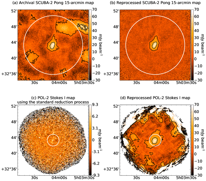
Figure 1: L 1512 JCMT 850 $\mu$m total intensity maps sampled on a 4^′′-grid. (a) Archival SCUBA-2 Pong-15^′ map from the makemap routine (see Sec. 2.1). (b) Reprocessed SCUBA-2 map from the skyloop routine with a PCA model (see Sec. 3.1). (c) POL-2 Stokes I map with the standard pol2map reduction process, including a PCA model, and (d) the reprocessed POL-2 Stokes I map from the makemap routine with the PCA model disabled (see Sec. 3.2). The uniform noise fields with diameters of 15^′ for SCUBA-2 and 3^′ for POL-2 are indicated by white circles. Panels other than (c) have the same color scales and same relative contour levels (20% and 60%) with respect to their peak intensities (74, 70, and 69 mJy beam^-1 for panels (a), (b), and (d)) for straightforward comparison. The color scale of panel (c) is [$-3\sigma$, $3\sigma$], where $\sigma=3.1$ mJy beam^-1 is measured in the central 3^′ field.

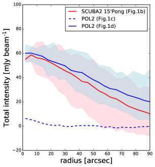
Figure 2: L 1512 850 $\mu$m total intensity profiles. The curves are averaged radial profiles while the filled areas show the ranges of the maximum and minimum intensities. The red curve and filled area show the profile of the SCUBA-2 map in Fig. 1b. The blue dashed curve shows the profile of the POL-2 Stokes I map in Fig. 1c. The blue solid curve and filled area show the profile of the POL-2 Stokes I map in Fig. 1d.

Figure 3: L 1512 JCMT 850 $\mu$m Stokes I, Q, and U maps. (a) SCUBA-2 4^′′-sampled map (a zoomed-in view of Fig. 1b) used as the input total intensity model (see Sec. 3.2) and (b) the same map but smoothed and sampled on a 12^′′-grid. Both maps are overlaid with contours at 0%, 20%, 40%, 60%, and 80% of their peak intensities. The B-field vectors (polarization vectors rotated by 90^∘) are overlaid on the 12^′′-grid, where vectors with polarization fraction SNR ($p/\sigma_{p}$) larger than 6 are shown in red and vectors with $6>p/\sigma_{p}\geq 3$ in blue. Vector lengths are scaled according to polarization fraction in panel (a), where a scale bar of 10% (or $p=0.1$ in a decimal equivalent) is denoted in the bottom right corner, and shown with uniform lengths in panel (b). (c) Stokes Q and (d) Stokes U 12^′′-sampled maps overlaid with the contours from panel (b). The beam sizes of 14^′′ are denoted in the bottom left corners. The 3^′ POL-2 uniform noise fields are indicated by white and black circles, in which the rms noises are measured as 4.35, 1.03, 0.79, and 0.79 mJy beam^-1 in panels (a)–(d), respectively.

2 Observations

2.1 James Clerk Maxwell Telescope (JCMT) Observations

The Submillimeter Common-User Bolometer Array 2 (SCUBA-2; Holland et al., 2013) photometric 850 $\mu$m observations of L 1512 were retrieved from the JCMT archive. They are part of the M13BC01 project (PI: James di Francesco) observed in November 2013. The raw data from six observations and one reduced image were downloaded. Each observation was integrated for 40 minutes with the PONG-900 scan pattern, which fully samples a 15^′ diameter circular region. The telescope beam size at 850 $\mu$m is 14^′′. The downloaded image is presented in Fig. 1a, showing some possibly spurious extended structures. This image was reduced by the pipeline using the iterative map-making routine makemap provided by the SMURF package in the Starlink software suite (Chapin et al., 2013). We applied another reduction routine on the raw data to eliminate the spurious structures and the details are described in Sec. 3.1.

For 850 $\mu$m polarization, we observed L 1512 with the POL-2 polarimeter (Friberg et al., 2016) mounted on the SCUBA-2 camera on JCMT. L 1512 was observed 27 times, for a total of 14 hours, between August 2020 to November 2020 in Band 2 weather (${0.05<\tau_{\rm 225GHz}<0.08}$) under project code M20BP046 (PI: Sheng-Jun Lin). Each observation was integrated for 31 minutes with the POL-2-DAISY scan pattern, which fully samples a 3^′ diameter circular region. The reduction details are described in Sec. 3.2.

2.2 Mimir Polarization Observations

We conducted H band polarization observations toward L 1512 on 2019 December 16, 17, and 20, and on 2020 January 6 and 9, and February 9 with the Mimir instrument (Clemens et al., 2007) mounted on the 1.8 m Perkins telescope outside Flagstaff, Arizona, U.S., operated by Boston University. Seeing conditions were between 1.6–3.4 arcsec for all observations. Data were calibrated with the Basic Data Processor (MSP-BDP) and Photo-Polarimetry Analysis Tool (MSP-PPOL) from the Mimir Software Package. The data selection criteria were that the H band magnitude was less than or equal to 13.5 mag, the polarization fraction uncertainty ($\sigma_{p}$) was less than or equal to 0.9% (or $\sigma_{p}\leq 0.009$ in a decimal equivalent), and an SNR of the polarization fraction ($p/\sigma_{p}$) $\geq 2$ or $\sigma_{\textit{PA}}\leq 15^{\circ}$, yielding a sample of 31 stars out of the 194 total observed.

2.3 Other Observations

Herschel 500 $\mu$m data with the beam size of 36^′′ (Observation ID: 1342191182, Quality: level 2 processed) were retrieved from the NASA/IPAC Infrared Science Archive. Planck 353 GHz (850 $\mu$m) polarization data were retrieved from the Planck Legacy Archive. We employed the Planck 2018 GNLIC Stokes I, Q, and U foreground thermal dust emission maps at variable resolution (5^′–80^′) over the sky (PR3; Planck Collaboration IV, 2020; Planck Collaboration XII, 2020), where the Galatic foreground emission is estimated by the GNLIC foreground dust model (Remazeilles et al., 2011), with reduced contamination from the cosmic infrared background, cosmic microwave background, and instrumental noise. The dataset we used for L 1512 has an effective beam size of 15^′.

3 Data Reduction

We describe our JCMT data reduction recipes and compare them to the standard processes in the following.

3.1 JCMT SCUBA-2 Photometric Map

Figure 1a shows the archival SCUBA-2 image with the possibly spurious extended structures (see Sec. 2.1). In order to improve the map quality, we reduced the raw SCUBA-2 data using the skyloop routine with a configuration file optimized for extended emission, provided by the SMURF package. With this configuration file, the skyloop routine performed principal component analysis (PCA) to remove correlated noise (see Chapin et al., 2013). Figure 1b shows this reprocessed map, where the spurious extended structures are now absent. The map was gridded to 4^′′ pixels and calibrated using a flux conversion factor (FCF) of 537 Jy pW^-1 (Dempsey et al., 2013).

3.2 Missing Flux of JCMT POL-2 for Extended Structures

The POL-2 polarization data were first reduced with the standard two-stage reduction process using the pol2map routine in the SMURF package, which includes a PCA model to remove correlated noise. Pattle et al. (2021) contains a detailed description of the standard POL-2 reduction process. Figure 1c presents the POL-2 total intensity map reduced with the above standard procedure, while Figure 1d presents the total POL-2 intensity map reduced from the same POL-2 data but with a different reduction procedure that excluded the default PCA model (described later in this section). In contrast to the obvious detection of L 1512 in the SCUBA-2 map (Fig. 1b, peak at 70 mJy beam^-1), we found that the dust emission of L 1512 is undetected in Stokes I (Fig. 1c) and neither Q nor U are detected with the standard POL-2 data reduction. Given the rms noise of 3.1 mJy beam^-1 measured in the central 3 arcmin field in the POL-2 map using the standard reduction, the dust emission peak of L 1512 should be detected with an SNR of $\sim$20 based on the SCUBA-2 map. Therefore, we suspected that the POL-2 scanning pattern or other instrument/reduction issues might have filtered out extended emission when observing low-surface-brightness objects.

One difference between observations with and without POL-2 is the scan speed. POL-2 contains a half-wave plate (HWP) and a grid analyzer to measure polarized light. The standard POL-2 observing mode (POL-2-DAISY) is a “scan and spin” mode, in which the telescope is continuously moving while the HWP spins (Friberg et al., 2016). The POL-2-DAISY scan speed is slow (8^′′ s^-1), which is limited by the integration time for a full polarization cycle (i.e., the HWP rotation speed of 2 Hz). Thus the data can be sufficiently sampled and the Stokes parameters Q and U can be registered to the maps with at least 4^′′ pixels, which is the default pixel size (about one-third of the 850 $\mu$m beam size of 14^′′; i.e., over-sampled by a factor of $\sim$1.5 relative to a standard Nyquist sampling rate) adopted by the pol2map routine. Such a slow speed could result in less extended structure recovery because the sensitivity of bolometers is limited by the low-frequency noise dominated by slow atmospheric variation between bolometer readouts (Chapin et al., 2013; Friberg et al., 2016).

One approach to evaluate this possibility would be to work with the observatory to perform POL-2 observations with the other scan patterns. An alternate approach is to disable the PCA model included in the standard two-stage reduction process. PCA can remove the correlated components of the bolometer readouts. However, it may be not a good solution for producing the extended structures because the real signal could be also correlated among the bolometers and hence is removed, as discussed by Chapin et al. (2013). The POL-2 map size is about half the size of the SCUBA-2 PONG-900 map, so the relative coverage of extended structures on the POL-2 map is larger than that of the SCUBA-2 map. As a result, these extended structures are sampled more with POL-2, producing more correlated signals among the bolometers for POL-2. This may explain why the PCA model can help to improve the SCUBA-2 map (Fig. 1b) but failed for the POL-2 map (Fig. 1c). We re-reduced the POL-2 raw data using the makemap routine without PCA and set flagslow=0.01 to take into account the slow scan speed used by POL-2 so that the data taken with the POL-2 scan speed will not be flagged and ignored when producing the map. This allows comparing the results of the standard two-stage process with and without PCA, to see what the impact of the PCA model is. The new reduction result is shown in Fig. 1d. Without the default PCA model, L 1512 appears in the new, but noisier, map with a similar peak intensity as seen in our reprocessed SCUBA-2 map (Fig. 1b).

Figure 2 shows the azimuthally-averaged intensity profiles of our improved SCUBA-2 map (Fig. 1b) compared to the (no PCA) POL-2 total intensity map (Fig. 1d). The intensity profiles are similar, showing evidence that we did detect the signal from L 1512 with POL-2, although we cannot rule out the possibility that parts of the emission were still filtered out. The standard POL-2 data reduction procedure incorporates the PCA model for the purpose of removing background signals. This step is particularly essential due to the non-uniform and radially dependent background variation within the POL-2 observing field. Given that all bolometers in POL-2 observe the same background but with time delays in the time-stream data, these signals are correlated and identified as such by PCA. The PCA approach does effectively address the background signal issue. However, the presence of extended structures also leads to correlated total intensity signals between bolometer readouts, and these are subsequently removed by the PCA model. The above experiment of not using the PCA model indicates that the Stokes I intensity from L 1512 could be recovered in the polarization data despite the limitations in map quality.

Therefore, the POL-2 missing flux issue in the total intensity of L 1512 is likely due to several factors: (1) The scan speed of 8^′′ s^-1 is slow, (2) The background variation is radially dependent in the POL-2 observations, and (3) L 1512 is faint and extended, resulting in a low surface brightness contrast.

On the other hand, the HWP rotation speed of 2 Hz provides a fast 8 Hz modulation of linear polarized intensity, making the signals of Stokes Q and U extractable (Friberg et al., 2016). However, POL-2 data reduction requires a total intensity (Stokes I) map to define the source region with a fixed SNR to enable reducing the Stokes Q and U signals. We thus used the reprocessed SCUBA-2 map (Fig. 1b and Fig. 3a for a zoomed-in view) as the input Stokes I model for the POL-2 data reduction instead of the POL-2 Stokes I map. The reduced Q and U maps were gridded to 4^′′ pixels and calibrated using a POL-2 FCF of 725 Jy pW^-1 (Dempsey et al., 2013; Friberg et al., 2016). This POL-2 data reduction, involving the use of an external SCUBA-2 map, was recommended upon the initial release of POL-2 for open use (Friberg et al., 2016). This procedure was employed in the first POL-2 850 $\mu$m polarization studies by Ward-Thompson et al. (2017); Pattle et al. (2017), which focused on the Orion A filament, marking the initial publication from the B-fields In STar-forming Region Observations (BISTRO) survey. The newer standard procedure, utilizing the POL-2 Stokes I map, was adopted in subsequent BISTRO publications shortly after Kwon et al. (2018), as the targeted objects typically exhibit notable brightness, thereby facilitating effective reduction based on the POL-2 Stokes I data.

Figure 3 shows the Stokes I, U, and Q maps, where the Stokes I maps are overlaid with B-field vectors. Panel (a) shows a zoomed-in view of 4^′′-sampled Fig. 1b, while panels (b), (c), and (d) are binned and sampled on 12^′′-grid. The polarization vectors were computed from the Stokes I, Q, and U maps on the 12^′′-grid to make each vector a nearly independent measurement (close to the resolution of 14^′′). Assuming dust grains are aligned with the magnetic field, the dust emission polarization at submm wavelengths is perpendicular to the plane-of-sky magnetic field, while the dust-extincted starlight polarization in the NIR is parallel to the plane-of-sky magnetic field (e.g., Andersson et al., 2015; Pattle et al., 2023). Thus the vectors overlaid on Fig. 3a and 3b were rotated 90^∘ so they may represent the plane-of-sky B-field direction. The vectors have been then filtered, based on the SNR of the polarization fraction being larger than three ($p/\sigma_{p}\geq 3$) and the SNR of the total intensity larger than ten ($I/\sigma_{I}\geq 10$). We note that a few vectors appear in the periphery with very high polarization fractions of about 50%. This is probably because the total intensity is underestimated, as the whole point of using a SCUBA-2 PONG observation is to maximize large-scale structure recovery, but the flux could still be missed, as L 1512 is fainter and more extended (i.e., low-contrast surface brightness) compared to the other starless cores which have had 850 $\mu$m polarization detection (see Sec. 1). The average rms noise of the Stokes Q and U maps over the central 3^′ field is $\sim$0.79 mJy for 12^′′ pixels. For the total intensity map, the average rms noise is $\sim$1.03 mJy for 12^′′ pixels. We note that the total intensity rms noise is not related to the Stokes Q and U rms noise because we used the total intensity map observed with SCUBA-2 instead of POL-2.

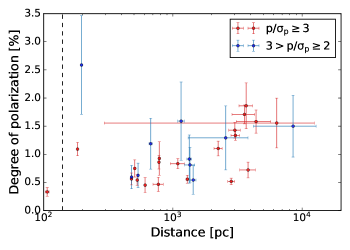
Figure 4: Mimir H band polarization fraction ($p$), expressed in percentage, is plotted against the stellar distance for 30 stars with positive parallax measurements ($\pi$) from Gaia DR3 (Gaia Collaboration, 2023), out of the total 31 stars. Dots with their uncertainties are shown in red for $p/\sigma_{p}\geq 3$, and in blue for $3>p/\sigma_{p}\geq 2$. The black dashed line indicates the nominal distance to L 1512 of 140 pc.

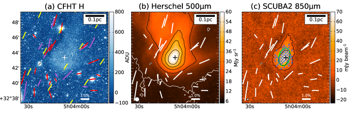
Figure 5: L 1512 Mimir H band background starlight polarimetry compared to dust maps. Mimir polarizations are shown as red, magenta, or white vectors on each panel with scale bars of 1% polarization fraction (or $p=0.01$ in a decimal equivalent). One star shows a grey vector as it is a foreground star, identified using Gaia data in Fig. 4. (a) CFHT H band image from Lin et al. (2020) and yellow Planck 353 GHz B-field vectors. The Mimir vectors are displayed in magenta for $3>p/\sigma_{p}\geq 2$ and in red for $p/\sigma_{p}\geq 3$. (b) Herschel 500 $\mu$m map with contours at 10, 20, 30, 40, and 50 MJy sr^-1. (c) JCMT SCUBA-2 850 $\mu$m map from Fig. 1b with contours at 10%, and 50% of the peak intensity at 69.5 mJy beam^-1. The 2D Gaussian intensity fitting result is denoted by a green ellipse. The JCMT 850 $\mu$m B-field vectors with $p/\sigma_{p}>3$ are displayed in blue with uniform lengths. The central cross in each panel indicates the center of L 1512 (Lin et al., 2020). The scale bars of 0.1 pc and submillimeter-wavelength beam sizes are denoted in the top right and bottom left corners, respectively.

3.3 Polarization Properties

The formulae for computing the polarization properties from the reduced data are as follows: the non-debiased polarization fraction ($p\mbox{${}^{\prime}$}$) is given by

$$p\mbox{${}^{\prime}$}=\frac{1}{I}\sqrt{Q^{2}+U^{2}},$$ (1)

where I, Q, U are the Stokes parameters measured. We let $\sigma_{I}$, $\sigma_{Q}$, and $\sigma_{U}$ be their uncertainties. Uncertainty of the polarization fraction ($\sigma_{p}$) is given by

$$\sigma_{p}=\sqrt{\frac{Q^{2}\sigma_{Q}^{2}+U^{2}\sigma_{U}^{2}}{I^{2}(Q^{2}+U^{2})}+\frac{(Q^{2}+U^{2})\sigma_{I}^{2}}{I^{4}}}.$$ (2)

The polarization fraction is debiased using the asymptotic estimator (Vaillancourt, 2006; Montier et al., 2015),

$$p=\sqrt{p\mbox{${}^{\prime}$}^{2}-\sigma_{p}^{2}},$$ (3)

and is rearranged by adopting the aforementioned ${\sigma_{Q}=\sigma_{U}=0.79}$ mJy beam^-1 and ignoring the $I^{-4}$ term of the radicand in Equation 2 (Kwon et al., 2018) as

$$p\approx\frac{1}{I}\sqrt{Q^{2}+U^{2}-\frac{1}{2}(\sigma_{Q}^{2}+\sigma_{U}^{2})},$$ (4)

where $p$ is the debiased polarization fraction. The polarization angle (PA) is given by

$$\textit{PA}=\frac{1}{2}\arctan{\left(\frac{U}{Q}\right)},$$ (5)

and the uncertainty of the polarization angle ($\sigma_{\textit{PA}}$) by

$$\sigma_{PA}=\frac{1}{2}\frac{\sqrt{Q^{2}\sigma_{U}^{2}+U^{2}\sigma_{Q}^{2}}}{Q^{2}+U^{2}}.$$ (6)

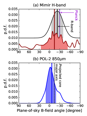
Figure 6: Probability density function (p.d.f.) of B-field position angles ($\theta$). The upper panel shows the Mimir data (red), while the lower panel shows the JCMT POL-2 data (blue). The mean and the 68% highest density interval (HDI) of the B-field angle distributions are displayed with vertical lines and filled areas. The Planck mean field angle of $-$30^∘ is plotted as a purple line in panel (a). The mean field angle, with standard deviation, of AIMPOL R-band polarizations Sharma et al. (2022) is represented as a Gaussian distribution on panel (a), vertically offset by a probability of 1% for clarity. The position angle of the core major axis ($\textit{PA}=-14.2^{\circ}$; see Fig. 5c) resulting from the 2D Gaussian fitting to the 850 $\mu$m intensity is plotted as a black dashed line in panel (b).

4 Results and analysis

4.1 Foreground Star Census

The dust-extincted starlight polarization in the Mimir H band from the background stars can trace the plane-of-sky magnetic field toward L 1512. We aim to identify and exclude foreground stars from our H band polarimetric detection. We match our 31 Mimir NIR stellar polarization measurements with the Gaia parallax ($\pi$) measurements (DR3; Gaia Collaboration, 2023). Figure 4 shows the H band polarization fraction ($p$) plotted against their stellar distance, except for one star with a negative parallax ($-0.0480\pm 0.2224$ mas). The stellar distance ($d$) is calculated by, $d=1/\pi$, and the corresponding uncertainty is approximated by $\sigma_{d}=\sigma_{\pi}/\pi^{2}$ (Luri et al., 2018). We adopt the nominal distance of 140 pc to L 1512 (Kenyon et al., 1994; Torres et al., 2009; Roccatagliata et al., 2020) and identify one foreground star with a distance of $107\pm 4$ pc. This foreground star indeed has the lowest H band polarization fraction among our data ($0.330\pm 0.077$%, expressed in percentage). The other 30 stars are categorized as background stars due to their distances being greater than $183\pm 1$ pc. Accordingly, they trace the magnetic field toward L 1512 because CO isotopologue line observations exhibit only one gas component along the sightlines (Falgarone et al., 1998). Figure 5a shows the Mimir H band polarization vectors superimposed on the CFHT H band image. A grey vector corresponds to the foreground star, while the remaining 30 vectors are associated with background stars. The sightlines toward these background stars sample from about 130^′′ away from the core center ($\text{R.A.}=5^{\mathrm{h}}04^{\mathrm{m}}07\fs 5$ and $\text{decl.}=32\arcdeg 43\mbox{${}^{\prime}$}25\farcs 0$, J2000; Lin et al., 2020) and continue out to 410^′′. Therefore, their polarization angles mostly trace the morphology of the plane-of-sky magnetic field in the diffuse envelope, spanning from a spatial scale of $\sim$0.56 pc down to $\sim$0.18 pc, which is the outer layers of the L 1512 cloud surrounding the dense core.

4.2 Magnetic Field Morphology

Figure 5 shows Mimir H band polarization (B-field) vectors overlaid on the continuum maps. These images trace different spatial structures of L 1512. Both the JCMT 850 $\mu$m and Herschel 500 $\mu$m dust emission trace the central cold dust. Herschel had much greater sensitivity to large-scale emission, while SCUBA-2 mostly traces the cold dust in the L 1512 core. The H band dust scattered light (cloudshine; Foster & Goodman, 2006) traces the L 1512 envelope (the outer diffuse region surrounding the L 1512 core; Saajasto et al., 2021).

The Mimir vectors mostly trace the magnetic field morphology in the diffuse envelope, with a spatial scale of $\sim$0.56 pc down to $\sim$0.18 pc (see Sec. 4.1). The envelope-scale B-field pattern seems to generally follow the large-scale magnetic field traced by the Planck 353 GHz (850 $\mu$m) data. These Planck vectors were rotated 90^∘ to represent the plane-of-sky B-field directions ($\theta=\textit{PA}+90^{\circ}$) and over-sampled for visualization, as the entire field of view (11.5^′ $\times$12^′) of Fig. 5a fits within one effective Planck beam size of 15^′. The Planck data indicate the large-scale mean field angle of $\theta_{\rm Planck}=-30^{\circ}$ over a spatial scale of $\sim$0.6 pc at the distance of 140 pc.

In the southern region of L 1512, there are significant deviations of the NIR vector orientations compared to the Planck vector orientations. For these NIR vectors, the absolute deviation of their polarization angles around the Planck mean field angle (i.e., $|\theta_{\rm H}-\theta_{\rm Planck}|$) ranges from a minimum of $6^{\circ}\pm 13^{\circ}$ to a maximum of $80^{\circ}\pm 8^{\circ}$, with the 68th percentile absolute deviation at 51^∘. In contrast, the northern NIR vectors show comparatively less deviation from the Planck mean field angle, with the 68th percentile absolute deviation at 18^∘. This indicates a B-field orientation transition from large- to envelope-scales. These deviations of the NIR vectors seem to show the effects of a relative motion between the surrounding medium and L 1512, and most of the interaction with the surrounding medium occurs in the south-southeast.

In highly extincted regions, NIR background starlight is faint and the corresponding NIR polarization is difficult to detect. To investigate the magnetic fields in the core, polarimetry at longer, submillimeter wavelengths is necessary. In Sec. 3.2, Figure 3b has shown the JCMT POL-2 B-field vectors overlaid on the 850 $\mu$m continuum map, zoomed to the core region. Unlike the envelope-scale B-field, the core-scale B-field morphology in L 1512 shows a much more ordered pattern in a nearly vertical orientation ($\theta_{\rm POL2}\approx 0^{\circ}$). We note that the pattern exhibits a mostly smooth change in position angle from $\theta_{\rm POL2}\approx 0^{\circ}$ in the northwest to $\approx$ $-30^{\circ}$ in the southeast, similar to the large-scale mean field angle of $-30^{\circ}$ seen in the Planck data. The POL-2 data may reveal a twist or kink in the plane-of-sky orientations in the core region, blended with the large-scale magnetic field. Figure 5c shows a spatial comparison between POL-2 vectors and Mimir vectors, where the POL-2 vectors are identical to those in Fig. 3b but undersampled by a factor of two for clarity. Their distinct different spatial coverages indeed show that the Mimir data trace the envelope-scale B-field while the POL-2 data trace the core-scale B-field.

To further compare the magnetic field orientations at different scales, Figure 6 shows the distributions of the plane-of-sky B-field position angle ($\theta$) estimated from our Mimir and POL-2 data plus the mean field angle inferred from the Planck data. These B-field angle probability density functions (p.d.f.) are derived to account for the uncertainties ($\sigma_{\textit{PA}}$) in the individual PA measurements via accumulation of the representative Gaussian distributions (Clemens et al., 2020). For POL-2 and Mimir data, the mean B-field angle and the 68% highest density interval (68% HDI; equivalent to one standard deviation of a Gaussian distribution) calculated from the p.d.f. are ${-7^{\circ}}_{-12^{\circ}}^{+18^{\circ}}$ and ${-15^{\circ}}_{-39^{\circ}}^{+40^{\circ}}$, respectively. In addition, the mean B-field angle with standard deviation of $-23^{\circ}\pm 17^{\circ}$ inferred from the AIMPOL R band polarization of 94 stars (Sharma et al., 2022) is also overplotted. The optical R band polarization traces the magnetic field beyond the region probed by our NIR H band polarization because the dust extincts more in the R band.

Both the AIMPOL data and Planck data trace the large-scale plane-of-sky magnetic field of L 1512, but with different resolutions. The Planck measurements, with their low spatial resolution of 15^′ and small optical depth at 850 $\mu$m (Planck Collaboration XII, 2020), not only average the polarization on a large scale toward the L 1512 cloud but also integrate it along the line of sight, weighting it by dust emission intensity. In contrast, the R band measurements could not be made toward the central $\sim$10^′ extincted area of the L 1512 cloud (see Fig. 4 of Sharma et al., 2022). However, the AIMPOL data coverage has a diameter of $\sim$20^′ ($\sim$0.8 pc at the distance of 140 pc). As a result, the magnetic field traced in R band spans a wide field, sampling primarily the outer low-density region, but with relatively higher resolution, depending on the R band background star distribution. Given that foreground and background stars can be identified, one can confidently associate the measured polarization with the cloud. Consequently, both the Planck and AIMPOL measurements effectively trace the large-scale magnetic field pattern and are consistent with each other toward the low-density periphery of the L 1512 cloud.

The magnetic field toward L 1512 shows a consistent average orientation from the large scale down to the core scale. The largest angular dispersion is seen in the H band data, related to the previously mentioned deviation of the NIR vectors in the southern region. In addition, Sharma et al. (2022) found that the R band polarization fraction is lower toward the southern region compared to the other surrounding regions. They suggested that it could be due to the lack of aligned grains owing to the different grain size distribution, collisional disalignment with gas, or the depolarization caused by a tangled B-field. Therefore, with these multiwavelength polarimetric data, magnetic fields are suggested to thread from the large scale to the dense core scale in L 1512, while the magnetic field could interact with the diffuse medium in the envelope scale.

The dust emission of L 1512 (Figs. 5b and 5c) shows an elongated, cometary morphology. We performed a 2D Gaussian intensity fitting on the 850 $\mu$m map. The fitting result is denoted by the green ellipse in Fig. 5c. The PA of the major axis is ${-14.2^{\circ}\pm 0.4^{\circ}}$, and the major and minor FWHM axes are ${141.2\mbox{${}^{\prime\prime}$}\pm 2.1\mbox{${}^{\prime\prime}$}}$ and ${86.2\mbox{${}^{\prime\prime}$}\pm 1.3\mbox{${}^{\prime\prime}$}}$ ($\sim$0.10 pc and $\sim$0.06 pc at the distance of 140 pc), respectively. The major axis of the projected core shape is parallel to the B-field orientation (see Fig. 6b) instead of being perpendicular to the magnetic field as suggested by the B-field-dominated core formation scenario at the core scale of $\sim$0.1 pc (e.g., Galli & Shu, 1993a; Li & Shu, 1996; Ciolek & Basu, 2000; Myers et al., 2018). This discrepancy can be attributed to the projection effect of a tri-axial core, as suggested by Basu (2000). Chen & Ostriker (2018) conducted a comprehensive analysis of turbulent MHD simulations and they discovered that dense cores do tend to be tri-axial, unlike the idealized oblate cores assumed in classical theories. Moreover, they observed that environmental factors, such as ram pressure or magnetic pressure, also play a crucial role in shaping dense cores.

4.3 Davis–Chandrasekhar–Fermi Analysis

The Davis–Chandrasekhar–Fermi (DCF; Davis, 1951; Chandrasekhar & Fermi, 1953) method is widely used to derive the plane-of-sky B-field strength ($B_{\rm pos}$) using linear polarization data. This method assumes that the turbulence is sub-Alfvénic and the magnetic field is frozen into the gas, so the non-thermal gas motions result in a distortion of the magnetic field. By measuring the dispersions in the non-thermal gas velocities and in the polarization position angles, the field strength is (Crutcher et al., 2004):

$$B_{\rm pos} =\mathrm{Q}\sqrt{4\pi\langle\rho\rangle}\frac{\sigma_{v,{\rm NT}}}{\delta\theta}\,\,{\rm(cgs\,\,units)}$$ (7)

$$\approx 9.3\sqrt{\langle n_{\rm H_{2}}\rangle/{\rm cm}^{-3}}\frac{\Delta v_{\rm NT}/{\rm km\cdot s^{-1}}}{\delta\theta/{\rm degree}}\,\,\mu G,$$ (8)

where $\langle\rho\rangle$ is the mean volume mass density, $\langle n_{\rm H_{2}}\rangle$ is the mean H₂ number density ($\langle\rho\rangle$ = $\mu_{\rm H_{2}}\langle n_{\rm H_{2}}\rangle m_{\rm H}$, and $\mu_{\rm H_{2}}$ = 2.8), $\sigma_{v,{\rm NT}}$ is the 1D non-thermal velocity dispersion, $\Delta v_{\rm NT}$ is the non-thermal FWHM linewidth ($\Delta v_{\rm NT}=\sigma_{v,{\rm NT}}\sqrt{8\log{2}}$), $\delta\theta$ is the intrinsic dispersion in B-field angles, and $\mathrm{Q}$ is a correction factor. Based on calibrations from numerical simulations (Heitsch et al., 2001; Ostriker et al., 2001), $\mathrm{Q}=0.5$ provides a good estimate of $B_{\rm pos}$, if $\delta\theta<25^{\circ}$.

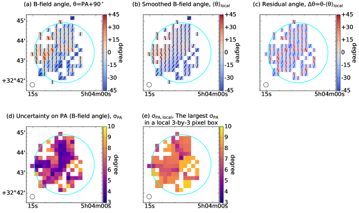
Figure 7: Position angles of the B-field orientations and their uncertainties. (a) B-field position angle map ($\theta$) inferred from the polarization angles (PA) rotated by 90^∘. (b) Mean B-field angle map ($\langle\theta\rangle_{\rm local}$) from convolving panel (a) by a boxcar filter with a size of 3-by-3 pixels. The black vectors overlaid on panels (a) and (b) show the B-field angles, while the magenta vectors on panel (b) show the mean B-field angles. (c) Residual map ($\Delta\theta=\theta-\langle\theta\rangle_{\rm local}$) and blue vectors of these residual angles are overlaid. (d) Uncertainty map ($\sigma_{\textit{PA}}$) of B-field angles. (e) Map of the local largest PA uncertainty ($\sigma_{\textit{PA},{\rm local}}$), on which each pixel value represents the largest PA uncertainty ($\sigma_{\textit{PA}}$) among the neighboring nine pixels within a 3-by-3 pixel box centered on that pixel. The “unsharp-masking method” sets the selection criteria based on $\sigma_{\textit{PA},{\rm local}}$ (see Sec. 4.3.1 and also Pattle et al., 2017). For panels (d) and (e), the minimum, mean, and maximum values are 3.5^∘, 5.9^∘, and 9.3^∘ for $\sigma_{\textit{PA}}$, and 4.7^∘, 7.6^∘, and 9.3^∘ for $\sigma_{\textit{PA},{\rm local}}$, respectively. The beam sizes are denoted in the bottom left corners. The 3^′ POL-2 uniform noise field is indicated by cyan circles.

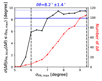
Figure 8: Residual angle ($\Delta\theta$) cumulative function of the maximum allowed B-field angle uncertainty ($\sigma_{\textit{PA},{\rm max}}$), in that the standard deviation of $\Delta\theta$ with the uncertainty ($\sigma_{\textit{PA},{\rm local}}$) equal to or less than $\sigma_{\textit{PA},{\rm max}}$ is evaluated. The standard deviation estimate, $\sigma(\Delta\theta)$, is shown as black dots, while the cumulative number of $\Delta\theta$ is shown as red dots. The intrinsic B-field angular dispersion ($\delta\theta$) of 8.2^∘$\pm$1.4^∘ (horizontal solid and dashed blue lines) is determined by computing the mean and standard deviation of the $\sigma(\Delta\theta)$ evaluated from $6^{\circ}\leq\sigma_{\textit{PA},{\rm max}}\leq 9.3^{\circ}$ (vertical dashed black lines).

4.3.1 Magnetic Field Angular Dispersion

We use the DCF method to estimate the plane-of-sky magnetic field strength at the core scale with the POL-2 data. The DCF method requires the intrinsic B-field angular dispersion measured from the random component of the magnetic field perturbed by local turbulence. However, the PA measurements include not just the random B-field component, but also the underlying ordered B-field component and the PA measurement uncertainties. Particularly, the core-scale B-field shows a slightly curved pattern by changing the B-field orientation from $\theta_{\rm POL2}\approx 0^{\circ}$ to $\theta_{\rm POL2}\approx-30^{\circ}$ in the southwestern side (see Fig. 3b). Thus, we adopt the “unsharp-masking method” (Pattle et al., 2017) to estimate the intrinsic angular dispersion of the random B-field component in L 1512. In this method, a smoothed B-field position angle map is created by convolving the original B-field angle map with a 3-by-3-pixel boxcar filter (i.e., a width of $\sim$2.6 independent beams). This smoothed map represents the underlying ordered B-field component. The 3-by-3-pixel boxcar filter minimizes the influence of the curvature of the field pattern. After subtracting this smoothed map from the original map, the residual angles represent the random B-field component and the PA measurement uncertainties. The intrinsic B-field angular dispersion can be estimated by the standard deviation of the residual angles.

Our analysis results for 850 $\mu$m are shown in Figs. 7 and 8. Figure 7a shows the B-field position angle ($\theta$) 12^′′-pixel map, where the vectors are shown with uniform lengths for clarity. Figure 7d shows the corresponding B-field-angle uncertainty ($\sigma_{\textit{PA}}$) map. We make a map of the underlying B-field by smoothing Fig. 7a with a 3-by-3-pixel boxcar filter (i.e., averaging over the nearby nine pixels). This smoothed B-field angle ($\langle\theta\rangle_{\rm local}$) map is shown in Fig. 7b. Figure 7c shows the residual ($\Delta\theta=\theta-\langle\theta\rangle_{\rm local}$) map, in which three isolated pixels from the $\theta$ and $\langle\theta\rangle_{\rm local}$ maps are rejected and 104 pixels remained.

On the residual angle map ($\Delta\theta$), the underlying ordered B-field geometry has been removed. In order to estimate a representative intrinsic B-field angular dispersion ($\delta\theta$) across L 1512, we present two approaches. One is the conventional approach, and the other one is a subsequent approach introduced in the unsharp-masking method. The conventional approach for estimating $\delta\theta$ is via the inverse-variance-weighted quadratic mean of the residual angles,

$$\delta\theta=\sqrt{\frac{\sum_{i}{w_{i}\Delta\theta_{i}^{2}}}{\sum_{i}{w_{i}}}},$$ (9)

where $w_{i}=1/\sigma_{\textit{PA},i}^{2}$ (e.g., Clemens et al., 2016; Wang et al., 2019). Hence the well-characterized residual angles with smaller $\sigma_{\textit{PA}}$ dominate the estimation. We find $\delta\theta=8.8^{\circ}\pm 0.5^{\circ}$ using this approach, where the uncertainty is calculated with the standard error propagation. On the other hand, Pattle et al. (2017) ran Monte Carlo simulations and demonstrated that a representative value of $\delta\theta$ can be better recovered, closer to the input $\delta\theta$ value in their simulations (their so-called “true value”), via averaging a set of standard deviation estimates of the residual angles selected with different maximum allowed PA uncertainties ($\sigma_{\textit{PA},{\rm max}}$); i.e., $\langle\sigma(\Delta\theta|{\rm uncertainties}\leq\sigma_{\textit{PA},{\rm max}})\rangle$. Figure 8 shows these standard deviation estimates as the function of $\sigma_{\textit{PA},{\rm max}}$, with black dots, and the cumulative number of the residual angles limited by $\sigma_{\textit{PA},{\rm max}}$, with red dots. Figure 7e shows the angular uncertainty of $\Delta\theta$, denoted by $\sigma_{\textit{PA},{\rm local}}$, adopted by Pattle et al. for this step. At each pixel, the $\sigma_{\textit{PA},{\rm local}}$ is the largest $\sigma_{\textit{PA}}$ of the neighboring nine pixels previously selected to compute $\langle\theta\rangle_{\rm local}$. Pattle et al. (2017) ran a set of Monte Carlo simulations by setting different “true values” of the intrinsic B-field angular dispersion ($\delta\theta$) to generate their simulated datasets. They found the above procedure can approach the input $\delta\theta$ when $\sigma_{\textit{PA},{\rm max}}$ is small and the cumulative number of $\Delta\theta$ is still sufficient. They took the mean of such well-characterized standard deviation estimates as the representative estimation of $\delta\theta$ for the whole region. In our analysis, we collect the standard deviation estimates computed with $6^{\circ}\leq\sigma_{\textit{PA},{\rm max}}\leq 9.3^{\circ}$ (two vertical dashed black lines in Fig. 8) because these $\sigma(\Delta\theta)$ estimates remain relatively similar values in contrast to the sharp $\sigma(\Delta\theta)$ decline at $\sigma_{\textit{PA},{\rm max}}<6^{\circ}$, which is due to the sample of the residual angles being too small (fewer than 6 vectors for this case). By taking the mean and standard deviation of these $\sigma(\Delta\theta)$ estimates, we obtain an intrinsic B-field angular dispersion ($\delta\theta$) of ${8.2^{\circ}\pm 1.4^{\circ}}$ (horizontal blue lines in Fig. 8) for the whole region. Compared to the conventional approach, both $\delta\theta$ estimations are consistent, and we adopt $\delta\theta=8.2^{\circ}\pm 1.4^{\circ}$ for the following analysis.

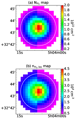
Figure 9: Density maps for the L 1512 core with $R_{\rm edge}$ = 108^′′. (a) $N_{\rm H_{2}}$ map. (b) Line-of-sight-averaged $n_{\rm H_{2}}$ map, on which each pixel is calculated as the column density divided by sightline depth. The 3^′ POL-2 uniform noise field is indicated by white circles for reference.

4.3.2 Number Density and Velocity Dispersion

Lin et al. (2020) built an onion-like volume density model of the L 1512 core, which is comprised of different eastern and western hemispheres. They modeled the density structure with Plummer-like profiles of $n_{0}/(1+(r/R_{0})^{\eta})$, where $n_{0}$ is the central density, $R_{0}$ is the characteristic radius, and $\eta$ is the power-law index of the density profile at $r\gg R_{0}$. The best-fit Plummer parameters fitted to N₂H⁺ spectral line observations and dust extinction measurements were found to be $n_{0}=1.1\times 10^{5}$ cm^-3, $R_{0}=0.022$ pc, and $\eta=2.0$ for the east side, and $n_{0}=1.1\times 10^{5}$ cm^-3, $R_{0}=0.027$ pc, and $\eta=3.1$ for the west side. Since the density required by the DCF method should be the average density along the line of sight, we assume the polarized light is mainly contributed by the L 1512 core, which has an $R_{\rm edge}$ of 108^′′ (= 0.073 pc; Lin et al., 2020). With the above density profiles, we (1) integrate the volume density profiles within the sphere defined by $R_{\rm edge}$ to obtain a column density ($N_{\rm H_{2}}$) map, and then (2) divide the column densities by the corresponding sightline depth inside the sphere to obtain the line-of-sight-averaged H₂ number density ($n_{\rm H_{2},los}$) map (i.e., for a pixel indexed $j$, $n_{{\rm H_{2},los},j}=N_{{\rm H_{2}},j}/(2\sqrt{R_{\rm edge,cm}^{2}-d_{j,{\rm cm}}^{2}})$, where $R_{\rm edge,cm}$ and $d_{j,{\rm cm}}$ are in the units of centimeter, and $d_{j,{\rm cm}}$ is the projected distance to the core center). Figure 9 shows the $N_{\rm H_{2}}$ map and $n_{\rm H_{2},los}$ map. For self-consistency, we compute the mean, and standard deviation, of $n_{\rm H_{2},los}$ and $N_{\rm H_{2}}$ values on the same set of pixels, of which the residual angles (Fig. 7c) are used to estimate the representative B-field angular dispersion $\delta\theta$. We find $\langle n_{\rm H_{2}}\rangle=\langle n_{\rm H_{2},los}\rangle=(2.1\pm 0.9)\times 10^{4}$ cm^-3, and $\langle N_{\rm H_{2}}\rangle=(8.3\pm 4.7)\times 10^{21}$ cm^-2. Lin et al. (2020) found that a non-thermal FWHM linewidth of $\Delta v_{\rm NT}=0.109$ km s^-1 can reproduce their N₂H⁺ (1–0) spectral observations. We take their N₂H⁺ (1–0) spectral resolution of 0.031 km s^-1 as the uncertainty. We adopt these values for the DCF analysis and list them in Table 1.

Table 1: Estimated properties in the DCF analysis from the 850 $\mu$m polarimetry.

Property	Value
$\delta\theta$ (degree)	$8.2^{\circ}\pm 1.4^{\circ}$
$\Delta v_{\rm NT}$ (km s-1)	$0.109\pm 0.031$
$\langle n_{\rm H_{2}}\rangle$ (cm-3)	$(2.1\pm 0.9)\times 10^{4}$
$\langle N_{\rm H_{2}}\rangle$ (cm-2)	$(8.3\pm 4.7)\times 10^{21}$
$B_{\rm pos}$ ($\mu$G)	$18\pm 7$
$\lambda_{\rm obs}$	$3.5\pm 2.4$
$|\textbf{B}_{\rm cor}|$ ($\mu$G)	$23\pm 9$
$\lambda_{\rm cor}$	$1.2\pm 0.8$
$B_{\rm tot}$ ($\mu$G)	$\sim$32
$B_{\rm los}$ ($\mu$G)	$\sim$27
$\lambda_{\rm tot}$	$\sim$1.6

4.3.3 Magnetic Field Strength and Mass-to-flux Ratio

Using the DCF method (Equation 8), and the above-estimated values (see Table 1), we calculate the mean plane-of-sky B-field strength ($B_{\rm pos}$) across the core to be $18\pm 7$ $\mu$G, where the uncertainty is computed with the standard error propagation from the dispersions of $\delta\theta$, $\Delta v_{\rm NT}$, and $n_{\rm H_{2}}$ and hence the uncertainty of $B_{\rm pos}$ represents the dispersion of its distribution.

It is also important to understand if the magnetic field could support the core against gravity, which can be determined by the mass-to-flux ratio in units of the critical ratio, $(M/\Phi)_{\rm crit}$. We use the formula from Crutcher et al. (2004),

$$\lambda=\frac{(M/\Phi)_{\rm obs}}{(M/\Phi)_{\rm crit}}=7.6\times 10^{-21}\frac{N_{\rm H_{2}}/{\rm cm}^{-2}}{B/{\rm\mu G}}.$$ (10)

The core is magnetically supercritical if $\lambda>1$ (i.e., unstable to collapse) and magnetically subcritical if $\lambda<1$ (i.e., magnetically supported). With our derived $\langle N_{\rm H_{2}}\rangle$ and $B_{\rm pos}$, we calculate the observed mass-to-flux ratio ($\lambda_{\rm obs}$) as $3.5\pm 2.4$ or a range of 1.1–5.9, suggesting that the magnetic field alone may not fully support the core against gravity. However, the mass-to-flux ratio could be overestimated by $\lambda_{\rm obs}$, due to the unknown inclination of the B-field and the 3D geometry of the core (Crutcher et al., 2004). On the other hand, the $\lambda_{\rm obs}$ lower limit of 1.1 does not entirely rule out the possibility of the magnetically critical condition, owing to various sources of uncertainty in the DCF method (Crutcher, 2012; Pattle & Fissel, 2019). Therefore, our estimation of the mass-to-flux ratio suggests that the L 1512 core is approximately magnetically critical or supercritical. We note that the mass-to-flux ratio calculated here is considered as a qualitative indicator rather than as a precise measure of the L 1512 core’s stability against gravity. We also note that when computing the mass-to-flux ratio, contributions from thermal and non-thermal energies are not considered.

Crutcher et al. (2004) showed that $B_{\rm pos}$ and $\lambda_{\rm obs}$ can be statistically corrected by averaging the cases of all B-field inclinations with respect to the line of sight. Under this methodology, $B_{\rm pos}$ is a statistical average of the total magnetic field, B_cor, which can point over a total solid angle of 2$\pi$ subtended from the core center. The correction is

$$B_{\rm pos}=\frac{\pi}{4}|\textbf{B}_{\rm cor}|.$$ (11)

In this case, the total magnetic field would have a strength of $23\pm 9$ $\mu$G. For our observed mass-to-flux ratio, $\lambda_{\rm obs}$, Crutcher et al. (2004) derived the correction as

$$\lambda_{\rm cor}=\frac{\lambda_{\rm obs}}{3}.$$ (12)

This correction also takes into account the projection effect of $N_{\rm H_{2}}$, assuming that the magnetic flux tube is aligned with the core minor axis. This yields a mass-to-flux ratio of $\lambda_{\rm cor}$ = $1.2\pm 0.8$, still suggesting the core is approximately magnetically critical or slightly supercritical. We will further discuss the B-field strength in the context of the Virial analysis in Sec. 5.

4.4 Grain Alignment

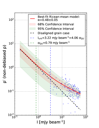
Figure 10: JCMT 850 $\mu$m non-debiased polarization fraction ($p\mbox{${}^{\prime}$}$) is plotted against the total intensity (Stokes I). The best-fit Ricean-mean model (Equation 14) and the grain disalignment model (Equation 15) are shown as solid red and dashed black lines, respectively. The red- and green-colored regions are the 68% and 95% confidence intervals, respectively.

A long-standing debate about submillimeter polarimetry is whether dust grains remain aligned with magnetic fields inside starless cores (e.g., Alves et al., 2014; Jones et al., 2015; Andersson et al., 2015; Wang et al., 2019; Pattle et al., 2019). From a theoretical standpoint, the main alignment mechanism is thought to be Radiative Alignment Torques (B-RATs), in which an anisotropic radiation field is a key to aligning the dust grains with the magnetic field (e.g., Dolginov & Mitrofanov, 1976; Lazarian & Hoang, 2007; Andersson et al., 2015). In the center of starless cores, the absence of an internal radiation source producing an anisotropic radiation field might lead to an outcome where dust grains are not aligned with the magnetic field. Therefore, it is crucial to investigate whether the dust grains are aligned at the centers of starless cores.

To evaluate grain alignment in the submillimeter regime, a power-law index in the $p-I$ relation,

$$p_{\rm true}(I)\propto I^{-\alpha},$$ (13)

is sought, where $0\leq\alpha\leq 1$ (e.g., Jones et al., 2015; Alves et al., 2015). In the $\alpha=0$ case, the polarization fraction is constant at every depth along each sightline, indicating a perfectly aligned case. For the $\alpha=1$ case, the polarized intensity ($=p_{\rm true}\cdot I$) is constant. In such a case, one interpretation is that only the outer shell of the starless core contributes to the polarized intensity, and no contribution comes from the inner region, implying a completely disaligned case (Pattle et al., 2019). We can only probe the B-field morphology at the core surface in this case.

In order to determine the index $\alpha$, we should take into account that the polarization fraction measurements do not follow a Gaussian distribution. Typically, the polarization fraction measurements are statistically debiased with a polarization estimator (e.g., the asymptotic estimator defined by Equation 3; please refer to Montier et al., 2015, for the detailed discussion of other estimators) and filtered with an SNR criterion for fitting $\alpha$. In fact, these polarization estimators are biased estimators but they work better in the high-SNR regime because the bias is minimized (Montier et al., 2015); therefore, the low-SNR data should be removed in order to better determine $\alpha$. For faint starless cores, such SNR criteria may remove too much data, and thus $\alpha$ might not be well-constrained.

Instead of debiasing data and removing the low-SNR ones, Pattle et al. (2019) assumed that the non-biased polarization fraction measurements follow a Rice distribution, including both low- and high-SNR data, and took the mean of the Rice distribution (Rice, 1945; Serkowski, 1958) as the estimator of the true polarization fraction at a given I. They referred to this estimator as the Ricean-mean model,

$$p\prime(I)=\sqrt{\frac{\pi}{2}}\left(\frac{I}{\sigma_{QU}}\right)^{-1}\mathcal{L}_{\frac{1}{2}}\left(-\frac{p_{\sigma_{QU}}^{2}}{2}\left(\frac{I}{\sigma_{QU}}\right)^{2(1-\alpha)}\right),$$ (14)

where $\mathcal{L}_{\frac{1}{2}}$ is a Laguerre polynomial of order 1/2, $\sigma_{QU}$ is the average of $\sigma_{Q}$ and $\sigma_{U}$, $\alpha$ is the power-law index, and $p_{\sigma_{QU}}$ is the expected polarization fraction when $I=\sigma_{QU}$. We note that technically, $p_{\sigma_{QU}}$ and $\sigma_{QU}$ are the free scaling factors of the assumed underlying $p-I$ relation of $p_{\rm true}=p_{\sigma_{QU}}(I/\sigma_{QU})^{-\alpha}$, where the I scaling factor is chosen to be the practical noise ($\sigma_{QU}$) while the polarization fraction scaling factor ($p_{\sigma_{QU}}$) is left for fitting. This Ricean estimator allows for a better estimation of the index $\alpha$ by being able to properly include the low-SNR data.

We use our data to determine the index $\alpha$ in L 1512 with the above Ricean-mean model. We collect data within a 3^′ uniform noise field (${\sigma_{QU}=0.79}$ mJy beam^-1), and supply $\sigma_{p}$ as a data weighting in order to perform a fitting with the Python scipy.optimize.curve_fit function. We obtain a best-fit $\alpha$ of ${0.48\pm 0.05}$, and $p_{\sigma_{QU}}$ of ${0.60\pm 0.10}$. Figure 10 shows the best-fit Ricean-mean model in the solid red curve. The true value of ${\alpha=0.48\pm 0.05}$ is recoverable above the critical intensity ($I_{\rm crit}$) of 3.22 mJy beam^-1 (corresponding to a SNR of $I_{\rm crit}/\sigma_{QU}=4.05$). In contrast, owing to the low SNR, the true $\alpha$ is not recoverable below $I_{\rm crit}$ but apparently approaches the value of unity expected for disaligned grains,

$$p\prime(I)=\sqrt{\frac{\pi}{2}}\left(\frac{I}{\sigma_{QU}}\right)^{-1},$$ (15)

shown as the dashed black line. The index of ${\alpha=0.48\pm 0.05}$ suggests that some of the dust grains remain aligned with the magnetic field at higher densities (Andersson et al., 2015; Pattle & Fissel, 2019). Therefore, our data are able to probe the magnetic field in the L 1512 core.

5 Discussion

5.1 Gravitational Stability

The gravitational stability of the L 1512 core can be assessed using the Virial theorem (McKee & Zweibel, 1992; McKee & Ostriker, 2007), which can be written as

$$\frac{1}{2}\frac{d^{2}I}{dt^{2}}=2(E_{\rm thermal}-E_{\rm surface}+E_{\rm turb}+E_{\rm rot})+E_{\rm grav}+E_{\rm mag},$$ (16)

where $I$ is the moment of inertia, $E_{\rm thermal}$ is the thermal energy in the core, $E_{\rm surface}$ is the surface kinetic term due to external pressure, $E_{\rm turb}$ is the turbulent energy, $E_{\rm rot}$ is the rotational energy, $E_{\rm grav}$ is the gravitational potential energy, and $E_{\rm mag}$ is the magnetic energy calculated by the total B-field strength ($B_{\rm tot}$). The magnetic energy can be divided into the plane-of-sky and line-of-sight components such that $E_{\rm mag}=E_{\rm mag,pos}+E_{\rm mag,los}$ since $B_{\rm tot}^{2}=B_{\rm pos}^{2}+B_{\rm los}^{2}$. The total kinetic energy can be defined as $T=E_{\rm thermal}-E_{\rm surface}+E_{\rm turb}+E_{\rm rot}$. By defining the virial energy of $E_{\rm vir}=2T+E_{\rm grav}$, we rewrite Equation 16 as

$$\frac{1}{2}\frac{d^{2}I}{dt^{2}}=E_{\rm vir}+E_{\rm mag,pos}+E_{\rm mag,los}.$$ (17)

The sign of $d^{2}I/dt^{2}$ determines whether the core is virially unbound with a positive net energy ($d^{2}I/dt^{2}>0$) or virially bound with a negative net energy ($d^{2}I/dt^{2}<0$), and $d^{2}I/dt^{2}=0$ means that the core is virially stable.

To assess the core stability, the physical structure of L 1512 is needed. Lin et al. (2020) focused on N₂H⁺ multi-transition spectra modeling and visual extinction measurement to build an onion model to describe the volume density, kinetic temperature, and rotational velocity profiles for the case of a constant turbulent velocity in the L 1512 core. Their onion model can well reproduce the N₂H⁺ and the other line data observed along a horizontal (RA) cut and a vertical (Dec) cut across the L 1512 core. The onion model is comprised of eastern (nine layers) and western (six layers) hemispheres, because the west extent of L 1512 is a factor of $\sim$2/3 shorter than along the eastern side. Here, we adopt the eastern hemisphere model to represent the entire core because the eastern side of L 1512 is more spherically symmetric with respect to the core center than the western side. Thus the eastern hemisphere onion model could provide a better description for the core (also see Figs. 1 and 2 from Lin et al., 2020).

Table 2: Energy budgets in L 1512.

Energy compared with $E_{\rm grav}$	Value
$E_{\rm grav}$ (erg)	$-3.9\times 10^{42}$
$E_{\rm thermal}/|E_{\rm grav}|$	0.61
$E_{\rm surface}/|E_{\rm grav}|$	0.41
$E_{\rm turb}/|E_{\rm grav}|$	0.04
$E_{\rm rot}/|E_{\rm grav}|$	0.01
$T/|E_{\rm grav}|$	0.25
$E_{\rm vir}/|E_{\rm grav}|$	$-$0.51
$E_{\rm mag,pos}/|E_{\rm grav}|$	0.16
$(E_{\rm vir}+E_{\rm mag,pos})/|E_{\rm grav}|$	$-$0.35

We use the physical parameters in the eastern onion model from Lin et al. (2020) to calculate each energy term in the Virial equation (Equation 16). Please refer to Table C.1 and Fig. 5c from Lin et al. (2020) for the density, temperature, and rotational velocity profiles. In addition, the constant one-dimensional non-thermal velocity dispersion, $\sigma_{v,{\rm NT}}$, used in the onion model is 0.046 km s^-1. We calculate the plane-of-sky component magnetic energy ($E_{\rm mag,pos}$) by using the DCF-derived plane-of-sky magnetic field strength ($B_{\rm pos}$) of 18 $\mu$G (Table 1). Table 2 summarizes the results for each energy of the L 1512 core and Appendix A shows the formulae we used for deriving each energy term. If we use the physical parameters in the western onion model from Lin et al. (2020), the virial energy ($E_{\rm vir}$) will change from $-$0.51 to $-$0.39 and the plane-of-sky component magnetic energy ($E_{\rm mag,pos}$) will change from 0.16 to 0.11, in units of $|E_{\rm grav}|$. Accordingly, if $E_{\rm mag,los}=0$, the value of the inertia term on the left-hand side of Equation 17 will change from $-$0.35 to $-$0.28 in units of $|E_{\rm grav}|$. We note that these energies could also have significant uncertainties; thus, these derived values are accurate only to order of magnitude. However, as the dominant uncertainty is mass, all the derived energies are linearly dependent on the mass, except that $E_{\rm grav}$ is dependent on the square of mass.

The rotational energy ($E_{\rm rot}$) in Table 2 is one of the interpretations from the N₂H⁺ (1–0) observation toward L 1512, which reveals a uniform velocity gradient (2.26$\pm$0.04 km s^-1 pc^-1) along roughly the north-south direction across an extent of $\sim 0.1$ pc (Caselli et al., 2002; Lin et al., 2020). An interpretation is a slow solid-body rotation (Caselli et al. 2002; Fig. 5c in Lin et al. 2020), of which the corresponding rotation period of 2.72$\pm$0.05 Myr ($\Omega=(7.3\pm 0.1)\times 10^{-14}$ rad s^-1 and $v_{\rm rot}\leq 0.07$ km s^-1) is about twice as long as the core lifetime of $\gtrsim$1.4 Myr (Lin et al., 2020). The corresponding $E_{\rm rot}$ is only 1% of $|E_{\rm grav}|$. This contribution does not affect the sign of $d^{2}I/dt^{2}$. Another interpretation involves the projection of tilted inward motions along filaments threaded by magnetic flux tubes (Balsara et al., 2001), which can be related to the slow, subparsec-scale accretion flows toward the core along the north-south CO filament (Falgarone et al., 2001). The blue- and red-shifted inward motions may lead to a kink of magnetic fields that contributes to the deviations of POL-2 polarization vectors from being uniform, as shown in Fig. 3b.

The plane-of-sky magnetic energy ($E_{\rm mag,pos}$) in Table 2 is calculated with the DCF-derived plane-of-sky B-field strength ($B_{\rm pos}$) of 18 $\mu$G. Because ${E_{\rm vir}+E_{\rm mag,pos}=-0.35|E_{\rm grav}|<0}$, the L 1512 core is virially bound if $E_{\rm mag,los}=0$, and further contraction could happen. However, the molecular spectral line observations toward L 1512 do not suggest that L 1512 is a “contracting core” but instead suggest it may have an “oscillating envelope.” Using the high-density tracer N₂H⁺ (1–0), Lin et al. (2020) performed non-LTE radiative transfer modeling and found no significant infall in the L 1512 core region. Employing the same radiative transfer model, we estimate an upper limit for the radial infall velocity of $\sim$0.04 km s^-1 by analyzing their N₂H⁺ data, indicating that the core region is relatively quiescent. Lin et al. also found that fitting their multi-line observations of N₂H⁺, N₂D⁺, DCO⁺, and o-H₂D⁺ does not require an infall velocity field in the radiative transfer model, even though the hyperfine structures were carefully considered. Additionally, the envelope of L 1512 was suggested to be oscillating because a mixture of blue and red asymmetric spectral line profiles was observed across the entire cloud in the CS (2–1) line (Lee & Myers, 1999; Lee et al., 2001; Lee & Myers, 2011), which is a low-density envelope tracer significantly depleted in the central core region. Another envelope tracer, HCN (1–0), which suffers fewer depletion effects compared with CS, also shows a mixed spectral feature across the observing area (Sohn et al., 2007; Kim et al., 2016). Although Schnee et al. (2013) found a red asymmetric feature from their HCO⁺ (3–2) observation, indicating an outward motion, their single-pointing observation does not conflict with the oscillation notion. Based on these spectral observations, L 1512 is likely a long-lived starless core, which is consistent with the core lifetime estimated to be longer than 1.4 Myr according to deuteration chemical modeling (Lin et al., 2020). Therefore, we expect the L 1512 core to be approximately virially stable. However, neither the kinetic pressure nor magnetic pressure of the plane-of-sky B-field alone can support the L 1512 core (i.e., $2T<|E_{\rm grav}|$ and $E_{\rm mag,pos}<|E_{\rm grav}|$). Given that the magnetic field seems to thread from the large scale to the core scale in L 1512, and the plane-of-sky magnetic field maintains a well-ordered field pattern, we speculate that the magnetic field is not entirely dynamically unimportant in the L 1512 core. It can be the case that the magnetic field does not lie close to the sky plane and a hitherto hidden line-to-sight magnetic field provides additional support, making L 1512 nearly stable. While Zeeman measurements of L 1512 would help to estimate the line-to-sight B-field strength, such a measurement is currently unavailable.

If the magnetic field is strong enough for the total magnetic energy to compensate for the negative $E_{\rm vir}$ value, leading the L 1512 core to be virially stable (i.e., ${0=\frac{1}{2}\frac{d^{2}I}{dt^{2}}=E_{\rm vir}+E_{\rm mag}}$ implies ${E_{\rm mag}=0.51|E_{\rm grav}|}$; see Appendix A), the total B-field strength ($B_{\rm tot}$) would need to be $\sim$32 $\mu$G. This strength is within the range measured in other starless cores derived via the DCF technique (e.g., Kirk et al., 2006; Pattle et al., 2021; Myers & Basu, 2021) and via the Zeeman effect technique (e.g., Crutcher & Troland, 2000; Troland & Crutcher, 2008). In this case, the line-of-sight B-field component ($B_{\rm los}=\sqrt{B_{\rm tot}^{2}-B_{\rm pos}^{2}}$) is estimated to be $\sim$27 $\mu$G and the inclination angle ($i=\sin^{-1}(B_{\rm pos}/B_{\rm tot})$) of total B-field direction is $\sim$34^∘ with respect to the line of sight. We note that the derived values of $B_{\rm tot}$ and $B_{\rm los}$, as well as the DCF-derived $B_{\rm pos}$ strength and energy budgets, carry certain uncertainties. It is better to consider that if $B_{\rm los}$ is present with a similar order of magnitude to $B_{\rm pos}=18\pm 7$ $\mu$G, these values suggest an approximate virial stability of L 1512. By adopting $N_{\rm H_{2}}=\langle N_{\rm H_{2}}\rangle\cos(i)$ and $B=B_{\rm tot}$ in Equation 10, the corresponding mass-to-flux ratio ($\lambda_{\rm tot}$) is $\sim$1.6, suggesting an approximately magnetically critical or sightly supercritical condition. Although $B_{\rm tot}$ does not make the L 1512 core magnetically subcritical, the magnetic pressure and the kinetic pressure are of comparable importance ($2T\sim E_{\rm mag}$ and $2T+E_{\rm mag}\sim|E_{\rm grav}|$) in supporting the core. On the other hand, if the magnetic fields in the L 1512 core do not have a line-of-sight component or just have a small $B_{\rm los}$, L 1512 would be magnetically supercritical and should be collapsing. However, the aforementioned spectral observations show this is not the case. Therefore, either L 1512 has just recently reached supercriticality and will collapse at any time and we happened to observe it in this special state, or L 1512 is nearly stable and there is an as-yet unseen line-of-sight B-field.

5.2 Relationship between Large- to Core-scale Magnetic Fields

The H band polarimetry is an important tool to trace the magnetic field at scales between those observed with POL-2 and with Planck. Our POL-2 850 $\mu$m, Mimir H band, and the Planck polarization observations enable efficient plane-of-sky B-field characterization across the small, intermediate, and large scales of the L 1512 cloud. As shown in Figs. 3 and 5, the magnetic field orientation of the L 1512 envelope (with an average field angle of $\theta_{\rm H}=-{15^{\circ}}_{-39^{\circ}}^{+40^{\circ}}$) appears to be inherited from that of the large-scale B-field ($\theta_{\rm Planck}=-30^{\circ}$) and reveals a twist in the B-field morphology between the core and the envelope. The twist occurs in the southwestern core region, where the field angle $\theta_{\rm POL2}$ bends from $\approx$$0^{\circ}$ in the core center to $\approx$$-30^{\circ}$, aligning with the nearby envelope-scale field at $\theta_{\rm H}\approx-30^{\circ}$ (see Sec. 4.2).

While the 3D field geometry of the field lines remains unknown, the observed twisted field may hint that the matter altered the field at the core scale of $\sim$0.1 pc, with the field orientation still close to the initial large-scale field. This suggests that L 1512 is likely in an intermediate phase, transitioning from the magnetically dominated phase (i.e., magnetically subcritical phase) to the matter-dominated phase (i.e., magnetically supercritical phase). This intermediate phase was proposed by Ward-Thompson et al. (2023) based on their polarimetric observations of nine starless cores embedded within the L 1495A-B10 filaments. The authors found that the plane-of-sky core-scale B-field orientations of these cores are roughly perpendicular to the filaments. However, they are not correlated with the large-scale B-field orientations measured by Planck, except for the lowest-density and possibly youngest core, where the core-scale field is still close to the large-scale field. In this case, a twisted field may be due to the early mass accumulation in the core, and the local field would become perpendicular to the major axis of the core if the gravitational instability is further enhanced.

On the other hand, twisted magnetic fields are also observed in protostellar sources such as filamentary gas flows on the subparsec scale in Serpens South (Pillai et al., 2020) and a twist of $\sim$45^∘ within the inner $\sim$0.005 pc region of L 483, a Class 0 protobinary core (Cox et al., 2022). These authors suggested that these twists result from the gas flow feeding onto the nearby cluster-forming regions and interactions involving binary systems. Thus, the aforementioned protostellar twists are formed in the magnetically supercritical phase, where gravity can efficiently influence the local magnetic field orientations. In contrast, the twist observed in L 1512 is likely developed during the intermediate phase.

In terms of kinematics, the L 1512 core exhibits quiescent gas motions. With the lack of significant gravitational instability, the magnetic field may be dynamically important in the core evolution of L 1512. Moreover, since the L 1512 cloud was reported to be magnetically subcritical based on R band data ($\lambda_{\rm obs}\sim 0.8$ at the scale of $\sim$0.8 pc; Sharma et al., 2022), the L 1512 core ($\lambda_{\rm obs}=3.5\pm 2.4$ and $\lambda_{\rm tot}\sim 1.6$ at the scale of $\sim$0.1 pc) may have undergone a sub-to-supercritical transition, through such as ambipolar diffusion.

As mentioned in Sec. 1, only a few starless cores have resolved submm polarization detections. Among these cores, L 183 (Clemens, 2012; Karoly et al., 2020), FeSt 1-457 (Alves et al., 2014; Kandori et al., 2017), and L 1544 (Clemens et al., 2016) also had polarization detection in the H band. In the cases of L 1544 and FeSt 1-457, despite the presence of some non-uniform B-field structures (Clemens et al., 2016; Alves et al., 2014), the orientations of their core-, envelope-, and large-scale magnetic fields remain roughly consistent, similar to L 1512. In contrast, L 183 is the only core in this sample where the orientation of the core-scale B-field tends to be perpendicular to that of the large-scale B-field; the transition of the B-field in the L 183 from its envelope to the core was captured by the H band polarization measurements (Clemens, 2012; Karoly et al., 2020). The apparently similar orientations in the large- and core-scale magnetic fields in L 1512, L 1544, and FeSt 1-457 (unless due to a projection effect) suggests that material can accrete onto these cores along magnetic field lines more efficiently than in the case in L 183. Such core formation scenario has been demonstrated by Chen et al. (2020) with their turbulent MHD simulations, suggesting that dense cores could accumulate more mass when the core-scale B-fields are aligned with the parsec-scale B-field. However, the L 183 cloud has a total mass of $\sim$80 M_⊙ (Pagani et al., 2004), which is considerably larger than the total mass of the L 1544 cloud, estimated to be $\sim$10 M_⊙ (Kim et al., 2022). It could be possible that the L 183 cloud is older, enabling it to accumulate sufficient mass, or that the L 183 cloud was supplied with a substantial ancient mass reservoir.

The potential transition from subcritical to supercritical magnetic conditions through ambipolar diffusion is a shared characteristic among L 1512, L 1544, and FeSt 1-457. This phenomenon has been proposed specifically for L 1544 (Ciolek & Basu, 2000; Li et al., 2002) and FeSt 1-457 (Kandori et al., 2020c; Bino & Basu, 2021). In terms of kinematics, L 1544 exhibits extended inward motions (Tafalla et al., 1998), whereas L 1512 and FeSt 1-457 have quiescent cores and oscillating envelopes (Aguti et al., 2007; Lee & Myers, 2011; Juárez et al., 2017; Lin et al., 2020). Moreover, FeSt 1-457 is suggested to be supported by both kinetic pressure and magnetic pressure (Kandori et al., 2018), similar to L 1512. In contrast, the entire L 183 core is found to be subcritical according to POL-2 observations (Karoly et al., 2020), suggesting the dominance of ambipolar diffusion in its core evolution. This could be consistent with the absence of inward motions for the L 183 core (Pagani et al., 2007) and that its surrounding envelope is suggested to be oscillating (Schnee et al., 2013). Despite that, the L 183 core has developed a central density ($2.3\times 10^{6}$ cm^-3; Pagani et al., 2007) comparable to that of L 1544 ($8.6\times 10^{6}$ cm^-3; Keto et al., 2015; Sipilä et al., 2022). Further observations of more starless cores remain vital to shed light on their core formation process and to better understand their environmental influences.

6 Conclusions

We present JCMT POL-2 850 $\mu$m dust continuum polarization observations and Mimir H-band NIR polarization observations toward L 1512. Our observations reveal an ordered core-scale B-field morphology in L 1512. From our analysis, we find the following:

1. The L 1512 850 $\mu$m data, as obtained, likely suffer from missing large-scale flux for the POL-2 data collection. We found that principal component analysis (PCA) in the standard reduction process removed extended emission, resulting in apparent non-detection of the total intensity. By including a SCUBA-2 Stokes I map in the reduction procedure, POL-2 Stokes Q and U maps could be correctly recovered.

2. The magnetic field traced by POL-2 850 $\mu$m, Mimir H band, AIMPOL R band, and Planck polarization data are in agreement as to the average field orientation, suggesting that the large-scale B-field threads the L 1512 cloud down into the dense core region. The largest angular dispersion, found in Mimir H band data, indicates that a transition of B-field morphology could be happening at the envelope scale.

3. Ricean-mean modeling of the non-debiased polarization fraction data yielded a power-law index $\alpha$ of 0.48$\pm$0.05 in the $p^{\prime}\propto I^{-\alpha}$ relation, indicating the dust grains retain substantial alignment with the magnetic field at the higher densities within the core.

4. A Davis–Chandrasekhar–Fermi analysis revealed a plane-of-sky B-field strength of 18$\pm$7 $\mu$G, and a mass-to-flux ratio of $\lambda_{\rm obs}=3.5\pm 2.4$ or a range of 1.1–5.9, suggesting that L 1512 is magnetically supercritical; however, the true mass-to-flux ratio may be being overestimated by $\lambda_{\rm obs}$, and the magnetically critical condition is not entirely ruled out. Given the absence of significant inward motions, and the presence of a well-ordered core-scale B-field and an oscillating envelope, it is likely that L 1512 is supported by both magnetic and kinetic pressures. By assuming L 1512 is virially stable and including the kinetic energy, we estimated that a total B-field strength of $\sim$32 $\mu$G could support the L 1512 core against gravity, suggesting a corresponding mass-to-flux ratio of $\sim$1.6. This requires a hitherto hidden line-of-sight B-field component of $\sim$27 $\mu$G, which could be sought using Zeeman effect techniques.

5. Alternatively, if there is little to no line-of-sight B-field, then L 1512 should be collapsing. In this case, L 1512 may have just recently reached supercriticality and will collapse at any time.

Appendix A Virial analysis

Here we present the equations for calculating each energy term in the Virial equation. For the ith layer in our onion model, we denote the H₂ number density as $n_{{\rm H_{2}},i}$, the temperature as $T_{{\rm kin},i}$, the inner and outer radii as $r_{i-1}$ and $r_{i}$, and the midpoint radius of the layer as $r_{i-\frac{1}{2}}=\frac{1}{2}(r_{i-1}+r_{i})$, where $i=1,...,N$, $r_{0}=0$, and $r_{N}=R$. The layer width is denoted as $\Delta r$.

We assume the gas is composed of molecular hydrogen, helium, and metals with the mass fractions of $X=0.7110$, $Y=0.2741$, and $Z=0.0149$, respectively (Lodders, 2003). The total number density, $n$, can be expressed as

$$n=n_{\rm H_{2}}+n_{\rm He}+n_{\rm metal}=\frac{\rho X}{2m_{\rm H}}+\frac{\rho Y}{4m_{\rm H}}+\frac{\rho Z}{15.5m_{\rm H}}=\frac{\rho}{m_{\rm H}}\left(\frac{X}{2}+\frac{Y}{4}+\frac{Z}{15.5}\right)=\frac{\rho}{m_{\rm H}}\frac{1}{\mu},$$ (A1)

where $\rho$ is volume mass density, $m_{\rm H}$ is the mass of the hydrogen atom and $\mu$ is the mean molecular weight per particle ($\mu=2.35$). The mean molecular weight per molecular hydrogen ($\mu_{\rm H_{2}}=2.81$) can be found by

$$n_{\rm H_{2}}=\frac{\rho X}{2m_{\rm H}}=\frac{\rho}{m_{\rm H}}\frac{1}{\mu_{\rm H_{2}}}.$$ (A2)

The volume mass density, $\rho$, can be expressed by either the total number density, $n$, or the H₂ number density, $n_{\rm H_{2}}$, with

$$\rho =\mu nm_{\rm H}$$ (A3)

$$=\mu_{\rm H_{2}}n_{\rm H_{2}}m_{\rm H}.$$ (A4)

The total number density, $n$, can be expressed by the H₂ number density, $n_{\rm H_{2}}$, with

$$n=\frac{\mu_{\rm H_{2}}}{\mu}n_{\rm H_{2}}.$$ (A5)

Another widely assumed gas composition is $n_{\rm H_{2}}=5n_{\rm He}$, where metals are negligible (e.g., Myers, 1983, and also the DCF formula of Equation 8). The corresponding mean molecular weights under this assumption are $\mu=2.33$ and $\mu_{\rm H_{2}}=2.8$. Although we adopt a different but more realistic gas composition in the Virial analysis from the one Crutcher et al. (2004) adopted in the DCF formula, the $\mu_{\rm H_{2}}$ from the two assumptions are similar and thus the derived volume mass density (Equation A4) would not have any significant difference.

We calculate the gravitational energy by

$$E_{\rm grav} =-4\pi\int_{0}^{R}GM(r)\rho(r)rdr$$ (A6)

$$\approx-4\pi G\mu_{\rm H_{2}}m_{\rm H}\sum_{i=1}^{N}M(r_{i-\frac{1}{2}})n_{{\rm H_{2}},i}r_{i-\frac{1}{2}}\Delta r,$$ (A7)

where $G$ is the gravitational constant, and $M(r)$ is the fractional core mass inside a radius of $r$.

We calculate the thermal energy by

$$E_{\rm thermal} =4\pi\int_{0}^{R}\frac{3}{2}n(r)k_{\rm B}T_{\rm kin}(r)r^{2}dr$$ (A8)

$$\approx 4\pi\frac{3\mu_{\rm H_{2}}k_{\rm B}}{2\mu}\sum_{i=1}^{N}n_{{\rm H_{2}},i}T_{{\rm kin},i}r_{i-\frac{1}{2}}^{2}\Delta r,$$ (A9)

where $k_{\rm B}$ is the Boltzmann constant.

The surface kinetic term due to external energy, $P_{\rm ext}$, is,

$$E_{\rm surface}=\frac{3}{2}P_{\rm ext}V=2\pi P_{\rm ext}R^{3},$$ (A10)

where $V$ is the core volume. Here we assume that $P_{\rm ext}=n_{\rm i=N}k_{\rm B}T_{\rm kin,i=N}$ is equal to the thermal pressure in the outermost layer.

In our onion model, the one-dimensional non-thermal velocity dispersion, $\sigma_{v,\rm NT}$, is a constant value of 0.046 km s^-1. The turbulent energy is calculated by

$$E_{\rm turb}=\frac{3}{2}M\sigma_{v,\rm NT}^{2},$$ (A11)

where $M$ is the total core mass.

The rotational energy is calculated by

$$E_{\rm rot}=\frac{1}{2}\sum_{i=1}^{N}I_{\rm i}\omega_{\rm i}^{2}=\frac{1}{2}\sum_{i=1}^{N}\frac{2}{5}(M(r_{i})-M(r_{i-1}))\frac{r_{i}^{5}-r_{i-1}^{5}}{r_{i}^{3}-r_{i-1}^{3}}\omega_{\rm i}^{2},$$ (A12)

where $I_{\rm i}$ and $\omega_{\rm i}$ are the moment of inertia and angular velocity of the $i$th layer, respectively.

The magnetic energy is calculated in the cgs units by

$$E_{\rm mag}=\frac{B^{2}}{8\pi}V.$$ (A13)

References

- Aguti et al. (2007) Aguti, E. D., Lada, C. J., Bergin, E. A., Alves, J. F., & Birkinshaw, M. 2007, ApJ, 665, 457, doi: 10.1086/519272
- Alves et al. (2014) Alves, F. O., Frau, P., Girart, J. M., et al. 2014, A&A, 569, L1, doi: 10.1051/0004-6361/201424678
- Alves et al. (2015) —. 2015, A&A, C4, doi: 10.1051/0004-6361/201424678e
- Andersson et al. (2015) Andersson, B. G., Lazarian, A., & Vaillancourt, J. E. 2015, ARA&A, 53, 501, doi: 10.1146/annurev-astro-082214-122414
- Astropy Collaboration et al. (2013) Astropy Collaboration, Robitaille, T. P., Tollerud, E. J., et al. 2013, A&A, 558, A33, doi: 10.1051/0004-6361/201322068
- Astropy Collaboration et al. (2018) Astropy Collaboration, Price-Whelan, A. M., SipHocz, B. M., et al. 2018, AJ, 156, 123, doi: 10.3847/1538-3881/aabc4f
- Balsara et al. (2001) Balsara, D., Ward-Thompson, D., & Crutcher, R. M. 2001, MNRAS, 327, 715, doi: 10.1046/j.1365-8711.2001.04787.x
- Basu (2000) Basu, S. 2000, ApJ, 540, L103, doi: 10.1086/312885
- Bino & Basu (2021) Bino, G., & Basu, S. 2021, ApJ, 911, 15, doi: 10.3847/1538-4357/abe6a4
- Caselli et al. (2002) Caselli, P., Benson, P. J., Myers, P. C., & Tafalla, M. 2002, ApJ, 572, 238, doi: 10.1086/340195
- Caselli et al. (2019) Caselli, P., Pineda, J. E., Zhao, B., et al. 2019, ApJ, 874, 89, doi: 10.3847/1538-4357/ab0700
- Chandrasekhar & Fermi (1953) Chandrasekhar, S., & Fermi, E. 1953, ApJ, 118, 116, doi: 10.1086/145732
- Chapin et al. (2013) Chapin, E. L., Berry, D. S., Gibb, A. G., et al. 2013, MNRAS, 430, 2545, doi: 10.1093/mnras/stt052
- Chapman et al. (2013) Chapman, N. L., Davidson, J. A., Goldsmith, P. F., et al. 2013, ApJ, 770, 151, doi: 10.1088/0004-637X/770/2/151
- Chen & Ostriker (2018) Chen, C.-Y., & Ostriker, E. C. 2018, ApJ, 865, 34, doi: 10.3847/1538-4357/aad905
- Chen et al. (2020) Chen, C.-Y., Behrens, E. A., Washington, J. E., et al. 2020, MNRAS, 494, 1971, doi: 10.1093/mnras/staa835
- Ching et al. (2017) Ching, T.-C., Lai, S.-P., Zhang, Q., et al. 2017, ApJ, 838, 121, doi: 10.3847/1538-4357/aa65cc
- Ciolek & Basu (2000) Ciolek, G. E., & Basu, S. 2000, ApJ, 529, 925, doi: 10.1086/308293
- Clemens (2012) Clemens, D. P. 2012, ApJ, 748, 18, doi: 10.1088/0004-637X/748/1/18
- Clemens et al. (2012) Clemens, D. P., Pavel, M. D., & Cashman, L. R. 2012, ApJS, 200, 21, doi: 10.1088/0067-0049/200/2/21
- Clemens et al. (2007) Clemens, D. P., Sarcia, D., Grabau, A., et al. 2007, PASP, 119, 1385, doi: 10.1086/524775
- Clemens et al. (2016) Clemens, D. P., Tassis, K., & Goldsmith, P. F. 2016, ApJ, 833, 176, doi: 10.3847/1538-4357/833/2/176
- Clemens et al. (2020) Clemens, D. P., Cashman, L. R., Cerny, C., et al. 2020, ApJS, 249, 23, doi: 10.3847/1538-4365/ab9f30
- Cox et al. (2022) Cox, E. G., Novak, G., Sadavoy, S. I., et al. 2022, ApJ, 932, 34, doi: 10.3847/1538-4357/ac722a
- Crutcher (2012) Crutcher, R. M. 2012, ARA&A, 50, 29, doi: 10.1146/annurev-astro-081811-125514
- Crutcher et al. (2004) Crutcher, R. M., Nutter, D. J., Ward-Thompson, D., & Kirk, J. M. 2004, ApJ, 600, 279, doi: 10.1086/379705
- Crutcher & Troland (2000) Crutcher, R. M., & Troland, T. H. 2000, ApJ, 537, L139, doi: 10.1086/312770
- Currie et al. (2014) Currie, M. J., Berry, D. S., Jenness, T., et al. 2014, in Astronomical Society of the Pacific Conference Series, Vol. 485, Astronomical Data Analysis Software and Systems XXIII, ed. N. Manset & P. Forshay, 391
- Davis (1951) Davis, L. 1951, Physical Review, 81, 890, doi: 10.1103/PhysRev.81.890.2
- Dempsey et al. (2013) Dempsey, J. T., Friberg, P., Jenness, T., et al. 2013, MNRAS, 430, 2534, doi: 10.1093/mnras/stt090
- Dolginov & Mitrofanov (1976) Dolginov, A. Z., & Mitrofanov, I. G. 1976, Ap&SS, 43, 291, doi: 10.1007/BF00640010
- Dunham et al. (2016) Dunham, M. M., Offner, S. S. R., Pineda, J. E., et al. 2016, ApJ, 823, 160, doi: 10.3847/0004-637X/823/2/160
- Eswaraiah et al. (2021) Eswaraiah, C., Li, D., Furuya, R. S., et al. 2021, ApJ, 912, L27, doi: 10.3847/2041-8213/abeb1c
- Falgarone et al. (1998) Falgarone, E., Panis, J.-F., Heithausen, A., et al. 1998, A&A, 331, 669
- Falgarone et al. (2001) Falgarone, E., Pety, J., & Phillips, T. G. 2001, ApJ, 555, 178, doi: 10.1086/321483
- Federrath & Klessen (2012) Federrath, C., & Klessen, R. S. 2012, ApJ, 761, 156, doi: 10.1088/0004-637X/761/2/156
- Foster & Goodman (2006) Foster, J. B., & Goodman, A. A. 2006, ApJ, 636, L105, doi: 10.1086/500131
- Friberg et al. (2016) Friberg, P., Bastien, P., Berry, D., et al. 2016, in Society of Photo-Optical Instrumentation Engineers (SPIE) Conference Series, Vol. 9914, Millimeter, Submillimeter, and Far-Infrared Detectors and Instrumentation for Astronomy VIII, ed. W. S. Holland & J. Zmuidzinas, 991403, doi: 10.1117/12.2231943
- Gaia Collaboration (2023) Gaia Collaboration. 2023, A&A, 674, A1, doi: 10.1051/0004-6361/202243940
- Galli & Shu (1993a) Galli, D., & Shu, F. H. 1993a, ApJ, 417, 220, doi: 10.1086/173305
- Galli & Shu (1993b) —. 1993b, ApJ, 417, 243, doi: 10.1086/173306
- Girart et al. (2009) Girart, J. M., Beltrán, M. T., Zhang, Q., Rao, R., & Estalella, R. 2009, Science, 324, 1408, doi: 10.1126/science.1171807
- Girart et al. (2006) Girart, J. M., Rao, R., & Marrone, D. P. 2006, Science, 313, 812, doi: 10.1126/science.1129093
- Goodman et al. (1995) Goodman, A. A., Jones, T. J., Lada, E. A., & Myers, P. C. 1995, ApJ, 448, 748, doi: 10.1086/176003
- Heitsch et al. (2001) Heitsch, F., Zweibel, E. G., Mac Low, M.-M., Li, P., & Norman, M. L. 2001, ApJ, 561, 800, doi: 10.1086/323489
- Holland et al. (2013) Holland, W. S., Bintley, D., Chapin, E. L., et al. 2013, MNRAS, 430, 2513, doi: 10.1093/mnras/sts612
- Hull & Zhang (2019) Hull, C. L. H., & Zhang, Q. 2019, Frontiers in Astronomy and Space Sciences, 6, 3, doi: 10.3389/fspas.2019.00003
- Hull et al. (2013) Hull, C. L. H., Plambeck, R. L., Bolatto, A. D., et al. 2013, ApJ, 768, 159, doi: 10.1088/0004-637X/768/2/159
- Jones et al. (2015) Jones, T. J., Bagley, M., Krejny, M., Andersson, B. G., & Bastien, P. 2015, AJ, 149, 31, doi: 10.1088/0004-6256/149/1/31
- Juárez et al. (2017) Juárez, C., Girart, J. M., Frau, P., et al. 2017, A&A, 597, A74, doi: 10.1051/0004-6361/201628608
- Kandori et al. (2017) Kandori, R., Tamura, M., Kusakabe, N., et al. 2017, ApJ, 845, 32, doi: 10.3847/1538-4357/aa7d58
- Kandori et al. (2018) Kandori, R., Tomisaka, K., Tamura, M., et al. 2018, ApJ, 865, 121, doi: 10.3847/1538-4357/aadb3f
- Kandori et al. (2020a) Kandori, R., Tamura, M., Saito, M., et al. 2020a, ApJ, 890, 14, doi: 10.3847/1538-4357/ab67c5
- Kandori et al. (2020b) —. 2020b, PASJ, 72, 8, doi: 10.1093/pasj/psz127
- Kandori et al. (2020c) Kandori, R., Tomisaka, K., Saito, M., et al. 2020c, ApJ, 888, 120, doi: 10.3847/1538-4357/ab6081
- Karoly et al. (2020) Karoly, J., Soam, A., Andersson, B. G., et al. 2020, ApJ, 900, 181, doi: 10.3847/1538-4357/abad37
- Karoly et al. (2023) Karoly, J., Ward-Thompson, D., Pattle, K., et al. 2023, ApJ, 952, 29, doi: 10.3847/1538-4357/acd6f2
- Kenyon et al. (1994) Kenyon, S. J., Dobrzycka, D., & Hartmann, L. 1994, AJ, 108, 1872, doi: 10.1086/117200
- Keto et al. (2015) Keto, E., Caselli, P., & Rawlings, J. 2015, MNRAS, 446, 3731, doi: 10.1093/mnras/stu2247
- Kim et al. (2016) Kim, G., Lee, C. W., Gopinathan, M., Jeong, W.-S., & Kim, M.-R. 2016, ApJ, 824, 85, doi: 10.3847/0004-637X/824/2/85
- Kim et al. (2022) Kim, S., Lee, C. W., Tafalla, M., et al. 2022, ApJ, 940, 112, doi: 10.3847/1538-4357/ac96e0
- Kirk et al. (2017) Kirk, H., Dunham, M. M., Di Francesco, J., et al. 2017, ApJ, 838, 114, doi: 10.3847/1538-4357/aa63f8
- Kirk et al. (2005) Kirk, J. M., Ward-Thompson, D., & André, P. 2005, MNRAS, 360, 1506, doi: 10.1111/j.1365-2966.2005.09145.x
- Kirk et al. (2006) Kirk, J. M., Ward-Thompson, D., & Crutcher, R. M. 2006, MNRAS, 369, 1445, doi: 10.1111/j.1365-2966.2006.10392.x
- Kwon et al. (2018) Kwon, J., Doi, Y., Tamura, M., et al. 2018, ApJ, 859, 4, doi: 10.3847/1538-4357/aabd82
- Launhardt et al. (2013) Launhardt, R., Stutz, A. M., Schmiedeke, A., et al. 2013, A&A, 551, A98, doi: 10.1051/0004-6361/201220477
- Lazarian & Hoang (2007) Lazarian, A., & Hoang, T. 2007, MNRAS, 378, 910, doi: 10.1111/j.1365-2966.2007.11817.x
- Lee & Myers (1999) Lee, C. W., & Myers, P. C. 1999, ApJS, 123, 233, doi: 10.1086/313234
- Lee & Myers (2011) —. 2011, ApJ, 734, 60, doi: 10.1088/0004-637X/734/1/60
- Lee et al. (2001) Lee, C. W., Myers, P. C., & Tafalla, M. 2001, ApJS, 136, 703, doi: 10.1086/322534
- Li et al. (2002) Li, Z.-Y., Shematovich, V. I., Wiebe, D. S., & Shustov, B. M. 2002, ApJ, 569, 792, doi: 10.1086/339353
- Li & Shu (1996) Li, Z.-Y., & Shu, F. H. 1996, ApJ, 472, 211, doi: 10.1086/178056
- Lin et al. (2020) Lin, S.-J., Pagani, L., Lai, S.-P., Lefèvre, C., & Lique, F. 2020, A&A, 635, A188, doi: 10.1051/0004-6361/201936877
- Liu et al. (2019) Liu, J., Qiu, K., Berry, D., et al. 2019, ApJ, 877, 43, doi: 10.3847/1538-4357/ab0958
- Lodders (2003) Lodders, K. 2003, ApJ, 591, 1220, doi: 10.1086/375492
- Lombardi et al. (2010) Lombardi, M., Lada, C. J., & Alves, J. 2010, A&A, 512, A67, doi: 10.1051/0004-6361/200912670
- Luri et al. (2018) Luri, X., Brown, A. G. A., Sarro, L. M., et al. 2018, A&A, 616, A9, doi: 10.1051/0004-6361/201832964
- Lynds (1962) Lynds, B. T. 1962, ApJS, 7, 1, doi: 10.1086/190072
- Mac Low & Klessen (2004) Mac Low, M.-M., & Klessen, R. S. 2004, Reviews of Modern Physics, 76, 125, doi: 10.1103/RevModPhys.76.125
- McKee & Ostriker (2007) McKee, C. F., & Ostriker, E. C. 2007, ARA&A, 45, 565, doi: 10.1146/annurev.astro.45.051806.110602
- McKee & Zweibel (1992) McKee, C. F., & Zweibel, E. G. 1992, ApJ, 399, 551, doi: 10.1086/171946
- Montier et al. (2015) Montier, L., Plaszczynski, S., Levrier, F., et al. 2015, A&A, 574, A136, doi: 10.1051/0004-6361/201424451
- Mouschovias (1991) Mouschovias, T. C. 1991, ApJ, 373, 169, doi: 10.1086/170035
- Mouschovias et al. (2006) Mouschovias, T. C., Tassis, K., & Kunz, M. W. 2006, ApJ, 646, 1043, doi: 10.1086/500125
- Myers (1983) Myers, P. C. 1983, ApJ, 270, 105, doi: 10.1086/161101
- Myers & Basu (2021) Myers, P. C., & Basu, S. 2021, ApJ, 917, 35, doi: 10.3847/1538-4357/abf4c8
- Myers et al. (2018) Myers, P. C., Basu, S., & Auddy, S. 2018, ApJ, 868, 51, doi: 10.3847/1538-4357/aae695
- Myers et al. (1983) Myers, P. C., Linke, R. A., & Benson, P. J. 1983, ApJ, 264, 517, doi: 10.1086/160619
- Ostriker et al. (2001) Ostriker, E. C., Stone, J. M., & Gammie, C. F. 2001, ApJ, 546, 980, doi: 10.1086/318290
- Padoan & Nordlund (1999) Padoan, P., & Nordlund, Å. 1999, ApJ, 526, 279, doi: 10.1086/307956
- Pagani et al. (2007) Pagani, L., Bacmann, A., Cabrit, S., & Vastel, C. 2007, A&A, 467, 179, doi: 10.1051/0004-6361:20066670
- Pagani et al. (2004) Pagani, L., Bacmann, A., Motte, F., et al. 2004, A&A, 417, 605, doi: 10.1051/0004-6361:20034087
- Pattle & Fissel (2019) Pattle, K., & Fissel, L. 2019, Frontiers in Astronomy and Space Sciences, 6, 15, doi: 10.3389/fspas.2019.00015
- Pattle et al. (2023) Pattle, K., Fissel, L., Tahani, M., Liu, T., & Ntormousi, E. 2023, in Astronomical Society of the Pacific Conference Series, Vol. 534, Astronomical Society of the Pacific Conference Series, ed. S. Inutsuka, Y. Aikawa, T. Muto, K. Tomida, & M. Tamura, 193
- Pattle et al. (2017) Pattle, K., Ward-Thompson, D., Berry, D., et al. 2017, ApJ, 846, 122, doi: 10.3847/1538-4357/aa80e5
- Pattle et al. (2019) Pattle, K., Lai, S.-P., Hasegawa, T., et al. 2019, ApJ, 880, 27, doi: 10.3847/1538-4357/ab286f
- Pattle et al. (2021) Pattle, K., Lai, S.-P., Di Francesco, J., et al. 2021, ApJ, 907, 88, doi: 10.3847/1538-4357/abcc6c
- Pillai et al. (2020) Pillai, T. G. S., Clemens, D. P., Reissl, S., et al. 2020, Nature Astronomy, 4, 1195, doi: 10.1038/s41550-020-1172-6
- Planck Collaboration IV (2020) Planck Collaboration IV. 2020, A&A, 641, A4, doi: 10.1051/0004-6361/201833881
- Planck Collaboration XII (2020) Planck Collaboration XII. 2020, A&A, 641, A12, doi: 10.1051/0004-6361/201833885
- Remazeilles et al. (2011) Remazeilles, M., Delabrouille, J., & Cardoso, J.-F. 2011, MNRAS, 418, 467, doi: 10.1111/j.1365-2966.2011.19497.x
- Rice (1945) Rice, S. O. 1945, The Bell System Technical Journal, 24, 46, doi: 10.1002/j.1538-7305.1945.tb00453.x
- Robitaille (2019) Robitaille, T. 2019, APLpy v2.0: The Astronomical Plotting Library in Python, doi: 10.5281/zenodo.2567476
- Robitaille & Bressert (2012) Robitaille, T., & Bressert, E. 2012, APLpy: Astronomical Plotting Library in Python, Astrophysics Source Code Library. http://ascl.net/1208.017
- Roccatagliata et al. (2020) Roccatagliata, V., Franciosini, E., Sacco, G. G., Randich, S., & Sicilia-Aguilar, A. 2020, A&A, 638, A85, doi: 10.1051/0004-6361/201936401
- Saajasto et al. (2021) Saajasto, M., Juvela, M., Lefèvre, C., Pagani, L., & Ysard, N. 2021, A&A, 647, A109, doi: 10.1051/0004-6361/202038401
- Schnee et al. (2013) Schnee, S., Brunetti, N., Di Francesco, J., et al. 2013, ApJ, 777, 121, doi: 10.1088/0004-637X/777/2/121
- Serkowski (1958) Serkowski, K. 1958, Acta Astron., 8, 135
- Sharma et al. (2022) Sharma, E., Gopinathan, M., Soam, A., Lee, C. W., & Seshadri, T. R. 2022, MNRAS, 517, 1138, doi: 10.1093/mnras/stac2487
- Shu et al. (1987) Shu, F. H., Adams, F. C., & Lizano, S. 1987, ARA&A, 25, 23, doi: 10.1146/annurev.aa.25.090187.000323
- Sipilä et al. (2022) Sipilä, O., Caselli, P., Redaelli, E., & Spezzano, S. 2022, A&A, 668, A131, doi: 10.1051/0004-6361/202243935
- Soam et al. (2018) Soam, A., Pattle, K., Ward-Thompson, D., et al. 2018, ApJ, 861, 65, doi: 10.3847/1538-4357/aac4a6
- Sohn et al. (2007) Sohn, J., Lee, C. W., Park, Y.-S., et al. 2007, ApJ, 664, 928, doi: 10.1086/519159
- Tafalla et al. (1998) Tafalla, M., Mardones, D., Myers, P. C., et al. 1998, ApJ, 504, 900, doi: 10.1086/306115
- Tassis & Mouschovias (2004) Tassis, K., & Mouschovias, T. C. 2004, ApJ, 616, 283, doi: 10.1086/424901
- Tokuda et al. (2020) Tokuda, K., Fujishiro, K., Tachihara, K., et al. 2020, ApJ, 899, 10, doi: 10.3847/1538-4357/ab9ca7
- Torres et al. (2009) Torres, R. M., Loinard, L., Mioduszewski, A. J., & Rodríguez, L. F. 2009, ApJ, 698, 242, doi: 10.1088/0004-637X/698/1/242
- Troland & Crutcher (2008) Troland, T. H., & Crutcher, R. M. 2008, ApJ, 680, 457, doi: 10.1086/587546
- Vaillancourt (2006) Vaillancourt, J. E. 2006, PASP, 118, 1340, doi: 10.1086/507472
- Virtanen et al. (2020) Virtanen, P., Gommers, R., Oliphant, T. E., et al. 2020, Nature Methods, 17, 261, doi: 10.1038/s41592-019-0686-2
- Wang et al. (2017) Wang, J.-W., Lai, S.-P., Eswaraiah, C., et al. 2017, ApJ, 849, 157, doi: 10.3847/1538-4357/aa937f
- Wang et al. (2019) —. 2019, ApJ, 876, 42, doi: 10.3847/1538-4357/ab13a2
- Ward-Thompson et al. (2000) Ward-Thompson, D., Kirk, J. M., Crutcher, R. M., et al. 2000, ApJ, 537, L135, doi: 10.1086/312764
- Ward-Thompson et al. (2009) Ward-Thompson, D., Sen, A. K., Kirk, J. M., & Nutter, D. 2009, MNRAS, 398, 394, doi: 10.1111/j.1365-2966.2009.15159.x
- Ward-Thompson et al. (2017) Ward-Thompson, D., Pattle, K., Bastien, P., et al. 2017, ApJ, 842, 66, doi: 10.3847/1538-4357/aa70a0
- Ward-Thompson et al. (2023) Ward-Thompson, D., Karoly, J., Pattle, K., et al. 2023, ApJ, 946, 62, doi: 10.3847/1538-4357/acbea4