Self-triggered Stabilization of Contracting Systems under Quantization

Abstract.

We propose self-triggered control schemes for nonlinear systems with quantized state measurements. Our focus lies on scenarios where both the controller and the self-triggering mechanism receive only the quantized state measurement at each sampling time. We assume that the ideal closed-loop system without quantization or self-triggered sampling is contracting. Moreover, a growth rate of the open-loop system is assumed to be known. We present two control strategies that yield the closed-loop stability without Zeno behavior. The first strategy is implemented under logarithmic quantization and imposes no time-triggering condition other than setting an upper bound on inter-sampling times. The second one is a joint design of zooming quantization and periodic self-triggered sampling, where the adjustable zoom parameter for quantization changes based on inter-sampling times and is also used for the threshold of self-triggered sampling. In both strategies, we employ a trajectory-based approach for stability analysis, where contraction theory plays a key role.

1. Introduction

Motivation and literature review

In modern control systems, shared networks and digital platforms are commonly used for implementing feedback laws. To effectively apply control theory in these systems, it is imperative to consider resource constraints, including bandwidth and processing power. Two crucial elements in these resource constraints are quantization and transmission frequency. Furthermore, it is important to be able to deal with nonlinear dynamics. This paper addresses these three aspects in a unified and systematic way.

Quantized control is motivated by numerous applications with limited communication capacity. The necessity for quantization also arises due to physical constraints on sensors and actuators. It has been shown in [14] that the coarsest quantization that quadratically stabilize a linear discrete-time system with a single input is logarithmic. In [16], an alternative proof for this result has been provided based on the sector bounded method. An adaptive control framework for continuous-time nonlinear uncertain systems with input logarithmic quantizers has been developed in [18]. Logarithmic quantizers have been applied to various classes of systems such as Markov jump time-delay systems [39] and parabolic partial differential equations [38, 22]. On the other hand, zooming quantizers, i.e., finite-level quantizers with adjustable zoom parameters have been developed for global asymptotic stabilization of linear systems in [6, 25]. This technique has been extended to nonlinear systems [24, 27], switched linear systems [26, 49], and so on. See also the overview [34] for quantized control.

The implementation of controllers on digital platforms requires time-sampling. While periodic sampling is straightforward to apply and is commonly used in control applications, it may lead to resource overconsumption. The need to use resources efficiently in networked control systems has motivated the study of event-based aperiodic sampling, which comprises two major sub-branches called event-triggered control [36, 37, 40, 19] and self-triggered control [46, 51, 3, 33]. In event-triggered control, sensors monitor the measurement data of the plant continuously or periodically and send the data to the controller only when the triggering condition is satisfied. To reduce the effort of monitoring the measurement data, self-triggering mechanisms (STMs) determine the next sampling times from the present (and past) measurement data at each sampling time.

For self-triggered control of nonlinear systems, various techniques have been introduced, e.g., approximation of isochronous manifolds [4, 11, 12], polynomial approximation of Lyapunov functions [5], and reduction of conservativeness through disturbance observers [43]. Approaches based on the small gain theorem [44, 29] and control Lyapunov functions [35] have been also discussed. In [42], an updating threshold strategy has been developed. A dynamic STM has been proposed in [21], by combing a hybrid Lyapunov function and a dynamic variable encoding the past system behavior. Moreover, self-triggered impulsive control for nonlinear time-delay systems has been applied to dose-regimen design in [2].

Numerous methods for quantized event-triggered control have been developed; see, e.g., [17, 23, 41, 13, 30, 1, 50, 15, 28] and the references therein. However, there are only a few approaches available for quantized self-triggered control. For continuous-time linear systems, a zooming quantizer and an STM have been jointly designed in [52], where the controller uses the quantized output whereas the STM relies on the non-quantized state. In [10], global exponential input-to-state stability with respect to bounded disturbances and noise has been achieved by a periodic STM for continuous-time linear systems. The joint design problem of a zooming quantizer and an STM using quantized measurements has been studied for discrete-time linear systems in [47, 31].

Problem description

All results developed in the above-mentioned studies on quantized self-triggered control are limited to linear systems. This study is one of the first step toward understanding nonlinear systems with quantization and self-triggered sampling. Of particular interest in this paper are contracting systems, i.e., systems whose flow is an infinitesimally contraction mapping. Contracting systems have highly-ordered asymptotic property and robustness against disturbances and noise. Contraction theory was initially introduced in [32] and has been the subject of extensive research since then; see the tutorial overview [45], the book [7], and the references therein. The norms we use for contractivity properties may be non-Euclidean. The non-Euclidean contraction framework has been established in [8, 9].

In this paper, we study the problem of self-triggered stabilization for contracting systems, where quantized state measurements at each sampling time are transmitted to the controller and the STM. Due to quantization and self-triggered sampling, the controller and the STM have access only to the limited information on the state. Throughout this paper, the measurement error means the difference between the unquantized value of the current state and the quantized value of the last measured state. Fig. 1 illustrates the closed-loop system we consider.

We assume that the following basic conditions are satisfied on a certain region containing the origin:

1. The ideal closed-loop system without quantization or sampling is contracting;

2. The growth rate of the open-loop system is bounded by a known constant; and

3. The function represented the dynamics of the ideal closed-loop system has a certain local Lipchitz property with respect to the measurement error.

By the first and third conditions, we guarantee that the state converges to the origin under quantization and self-triggered sampling. On the other hand, the second condition is used to estimate the magnitude of the measurement error for the computation of the next sampling time.

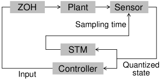
Figure 1. Closed-loop system.

Difficulties and contributions

The difficulties of the stabilization problem are as follows.

• Only the quantized data on the state can be used for the computation of the next sampling time. Model uncertainties and disturbances have been dealt with in the above-mentioned studies on self-triggered control for nonlinear systems. However, the techniques proposed in these studies cannot be directly applied to self-triggered sampling based on quantized data. Moreover, quantizer saturation may occur when a zooming quantizer is used. If the quantizer saturates, then the quantization error becomes large, and STMs designed for the ideal situation without quantization may lead to instability.

• For practical implementation, we have to ensure that inter-sampling times are bounded from below by a strictly positive constant. In the previous studies [10, 47, 28] on self-triggered sampling based on quantized or noisy data, inter-sampling times are chosen from a finite discrete set, and hence the minimum inter-sampling time has not been investigated. Since the measurement error is nonzero even at the sampling time due to quantization, it is more challenging to avoid Zeno behavior.

• We assume only local properties of the system behavior. The system has Lipschitz continuity with respect to the state only on a specific region and hence lacks, in general, fundamental properties such as the uniqueness of solutions outside that region. The state trajectory of the ideal closed-loop system stays in the region due to the contractivity property. However, when quantization errors and inter-sampling times are large, the state trajectory may leave this region.

Our initial focus is on self-triggered control under logarithmic quantization. The main objective of the STM is to check whether the measurement error exceeds a threshold like standard triggering mechanisms. To this end, the STM predicts the state from its quantized data at the latest sampling time and monitors whether the predicted state leaves the region where a uniform growth rate of the open-loop system is known. To employ local properties of the system behavior, the norm of the initial state is assumed to be upper-bounded by a given constant. Then we show that when the quantization density and the threshold parameter of self-triggered sampling satisfy suitable conditions, the closed-loop system has the following two properties: (i) the minimum inter-sampling time is lower-bounded by a strictly positive constant; (ii) the state norm decreases monotonically and exponentially.

Our second contribution is to propose a joint design method of a zooming quantizer and an STM. The STM checks the conditions on the measurement error and the predicted state as in the case of logarithmic quantization. The major difference is that the zooming quantizer and the STM update their parameters in relation to each other. In fact, depending on inter-sampling times, the zoom parameter of the quantizer is decreased in such a way as to drive the state to the origin. On the other hand, the STM uses the zoom parameter for a threshold. Since the periodic STM is applied, Zeno behavior does not occur. However, the period of the STM has to be small enough to guarantee the state convergence. We provide a sufficient condition for stabilization, which is described by inequalities with respect to the parameters for the range and step of quantization and for the threshold and period of self-triggered sampling.

Paper organization

The rest of this article as follows. In Section 2, basic assumptions on the nonlinear system we consider are discussed. Then we present preliminary results on the open-loop dynamics in Section 3. In Section 4, we propose a self-triggered stabilization scheme under logarithmic quantization. Section 5 is devoted to the problem of jointly designing a zooming quantizer and an STM. In Section 6, we consider Lur’e systems for the application of the proposed methods. We give a numerical example in Section 7. Finally, Section 8 concludes this article.

Notation

If a function $f\colon\mathbb{R}^{n}\to\mathbb{R}^{n}$ is differentiable at $x\in\mathbb{R}^{n}$, then we denote the Jacobian matrix of $f$ at $x$ by $Df(x)$. For a matrix $A\in\mathbb{R}^{n\times n}$ with $ij$-th element $A_{ij}$, the $ij$-th element of the Metzler majorant $\lceil A\rceil_{\mathrm{Mzr}}\in\mathbb{R}^{n\times n}$ of $A$ is defined by

$$(\lceil A\rceil_{\mathrm{Mzr}})_{ij}\coloneqq\begin{cases}A_{ij}&\text{if $i=j$}\\ |A_{ij}|&\text{if $i\not=j$}.\end{cases}$$

The elementwise inverse of a vector $\theta=[\theta_{1}~{}\cdots~{}\theta_{n}]^{\top}\in\mathbb{R}^{n}_{>0}$ is denoted by $\theta^{-1}$, i.e., $\theta^{-1}\coloneqq[\theta_{1}^{-1}~{}\cdots~{}\theta_{n}^{-1}]^{\top}$. For a vector $\theta\in\mathbb{R}^{n}$, let $[\theta]\in\mathbb{R}^{n\times n}$ denote the diagonal matrix whose $i$-th diagonal element is equal to the $i$-th element of $\theta$. When $\theta\in\mathbb{R}^{n}_{>0}$, we define the $\theta$-diagonally-weighted 1-norm and $\infty$-norm on $\mathbb{R}^{n}$ by

$$\|x\|_{1,\theta}\coloneqq\big{\|}[\theta]x\big{\|}_{1}\quad\text{and}\quad\|x\|_{\infty,\theta}\coloneqq\big{\|}[\theta]x\big{\|}_{\infty},\quad x\in\mathbb{R}^{n},$$

respectively. Let $\|\cdot\|_{*}$ be a norm on $\mathbb{R}^{n}$ and its corresponding induced norm on $\mathbb{R}^{n\times n}$. The logarithmic norm of a matrix $A\in\mathbb{R}^{n\times n}$ with respect to the norm $\|\cdot\|_{*}$ is written as

$$\mu_{*}(A)\coloneqq\lim_{\varepsilon\to 0+}\frac{\|I+\varepsilon A\|_{*}-1}{\varepsilon}.$$

For $R\in\mathbb{R}_{>0}\cup\{\infty\}$, we define the open ball $\mathbf{B}_{*}(R)$ with respect to the norm $\|\cdot\|_{*}$ by

$$\mathbf{B}_{*}(R)\coloneqq\begin{cases}\{x\in\mathbb{R}^{n}:\|x\|_{*}<R\}&\text{if $0<R<\infty$}\\ \mathbb{R}^{n}&\text{if $R=\infty$},\end{cases}$$

and denote its closure by $\overline{\mathbf{B}}_{*}(R)$.

2. Basic assumptions and system properties

In this section, we first discuss basic assumptions on the closed-loop system and the open-loop system. Then we present useful results obtained under those assumptions. These results give growth and decay properties of the systems and are fundamental to the design of STMs and the stability analysis of quantized self-triggered control systems.

2.1. Assumptions on non-linear systems

Throughout this paper, let $f\colon\mathbb{R}^{n}\times\mathbb{R}^{m}\to\mathbb{R}^{n}$ and $g\colon\mathbb{R}^{n}\to\mathbb{R}^{m}$ be continuous functions satisfying $f(0,g(0))=0$. Consider the ordinary differential equation (ODE)

$$\dot{x}(t)=f\big{(}x(t),u(t)\big{)},\quad t\in\mathbb{R}_{\geq 0};\qquad x(0)=x_{0}\in\mathbb{R}^{n},$$

where $x(t)\in\mathbb{R}^{n}$ and $u(t)\in\mathbb{R}^{m}$ are the state and the input of the nonlinear system at time $t$, respectively. In the ideal case without quantization or self-triggered sampling, the input $u$ is generated by the following controller:

$$u(t)=g\big{(}x(t)\big{)},\quad t\in\mathbb{R}_{\geq 0}.$$

For $x,e\in\mathbb{R}^{n}$, we define

$$F(x,e)\coloneqq f\big{(}x,g(x+e)\big{)}\quad\text{and}\quad F_{0}(x)\coloneqq F(x,0).$$

The ideal closed-loop dynamics is given by the ODE $\dot{x}=F_{0}(x)$. First, we make the following assumption on $F_{0}$ for the contractivity of the ideal closed-loop system.

Assumption 2.1.

There exist a norm $\|\cdot\|_{\mathop{\textrm{cl}}\nolimits}$ on $\mathbb{R}^{n}$ and constants $c\in\mathbb{R}_{>0}$ and $R_{1}\in\mathbb{R}_{>0}\cup\{\infty\}$ such that

1. $F_{0}$ is locally Lipschitz continuous on $\mathop{\mathbf{B}}_{\mathop{\textrm{cl}}\nolimits}\nolimits(R_{1})$; and

2. $\mu_{\mathop{\textrm{cl}}\nolimits}(DF_{0}(x))\leq-c$ for almost all $x\in\mathop{\mathbf{B}}_{\mathop{\textrm{cl}}\nolimits}\nolimits(R_{1})$.

Note that if $F_{0}$ is locally Lipschitz continuous on $\mathop{\mathbf{B}}_{\mathop{\textrm{cl}}\nolimits}\nolimits(R_{1})$, then $F_{0}$ is differentiable almost everywhere on $\mathop{\mathbf{B}}_{\mathop{\textrm{cl}}\nolimits}\nolimits(R_{1})$ by Rademacher’s theorem; see, e.g., [20, Theorem 6.15].

For a fixed $q\in\mathbb{R}^{n}$, we set

$$f_{q}(x)\coloneqq f\big{(}x,g(q)\big{)},\quad x\in\mathbb{R}^{n}.$$

When the input $u$ is a constant function such that $u(t)\equiv g(q)$ for some $q\in\mathbb{R}^{n}$, the open-loop dynamics is given by the ODE $\dot{x}=f_{q}(x)$. Next, we assume that $f_{q}$ satisfies the following properties, which gives a uniform growth bound of the open-loop system.

Assumption 2.2.

There exists a norm $\|\cdot\|_{\mathop{\textrm{op}}\nolimits}$ on $\mathbb{R}^{n}$ and constants $d_{1}\in\mathbb{R}_{\geq 0}$, $d_{2}\in\mathbb{R}_{>0}$, and $R_{2}\in\mathbb{R}_{>0}\cup\{\infty\}$ such that

1. $f_{q}$ is continuously differentiable on $\mathop{\mathbf{B}}_{\mathop{\textrm{op}}\nolimits}\nolimits(R_{2})$ for all $q\in\mathop{\mathbf{B}}_{\mathop{\textrm{op}}\nolimits}\nolimits(R_{2})$;

2. $\mu_{\mathop{\textrm{op}}\nolimits}(Df_{q}(x))\leq d_{1}$ for all $x,q\in\mathop{\mathbf{B}}_{\mathop{\textrm{op}}\nolimits}\nolimits(R_{2})$; and

3. $\|f_{q}(q)\|_{\mathop{\textrm{op}}\nolimits}\leq d_{2}\|q\|_{\mathop{\textrm{op}}\nolimits}$ for all $q\in\mathop{\mathbf{B}}_{\mathop{\textrm{op}}\nolimits}\nolimits(R_{2})$.

For the norms $\|\cdot\|_{\mathop{\textrm{cl}}\nolimits}$ and $\|\cdot\|_{\mathop{\textrm{op}}\nolimits}$ in Assumptions 2.1 and 2.2, let a constant $\Gamma\in\mathbb{R}_{>0}$ satisfy

$$\|x\|_{\mathop{\textrm{op}}\nolimits}\leq\Gamma\|x\|_{\mathop{\textrm{cl}}\nolimits}$$

and put

$$R\coloneqq\min\left\{R_{1},\frac{R_{2}}{\Gamma}\right\}.$$

Then

$$\mathop{\mathbf{B}}_{\mathop{\textrm{cl}}\nolimits}\nolimits(R)\subseteq\mathop{\mathbf{B}}_{\mathop{\textrm{cl}}\nolimits}\nolimits(R_{1})\cap\mathop{\mathbf{B}}_{\mathop{\textrm{op}}\nolimits}\nolimits(R_{2}).$$

As long as the state belongs to $\mathop{\mathbf{B}}_{\mathop{\textrm{cl}}\nolimits}\nolimits(R)$, the system properties in Assumptions 2.1 and 2.2 are satisfied. Therefore, we will design STMs so that the state of the quantized self-triggered control system does not leave $\mathop{\mathbf{B}}_{\mathop{\textrm{cl}}\nolimits}\nolimits(R)$.

Finally, we assume that the function $F(x,e)$ has a certain local Lipschitz property in the second argument $e$. This Lipschitz property will be used for upper-bounding the effect of the measurement error.

Assumption 2.3.

There exists constants $\alpha,\sigma_{0}\in\mathbb{R}_{>0}$ such that

(1) $$\|F(x,e)-F(x,0)\|_{\mathop{\textrm{cl}}\nolimits}\leq\alpha\|e\|_{\mathop{\textrm{op}}\nolimits}$$

for all $x\in\mathop{\mathbf{B}}_{\mathop{\textrm{cl}}\nolimits}\nolimits(R)$ and $e\in\mathop{\mathbf{B}}_{\mathop{\textrm{op}}\nolimits}\nolimits(\sigma_{0}R)$.

Note that the norm $\|\cdot\|_{\mathop{\textrm{op}}\nolimits}$ in Assumption 2.2 might differ from the norm $\|\cdot\|_{\mathop{\textrm{cl}}\nolimits}$ in Assumption 2.1. The norm $\|\cdot\|_{\mathop{\textrm{cl}}\nolimits}$ is applied for stability analysis of the quantized self-triggered control system, whereas the proposed STM estimates the magnitude of the measurement error by using the norm $\|\cdot\|_{\mathop{\textrm{op}}\nolimits}$. In the inequality of Assumption 2.3, the left-hand term relates to stability analysis and the right-hand term is associated with the measurement error. Consequently, this inequality is described by the two norms.

2.2. Growth and decay properties

The contraction theory provides a decay property of the ideal closed-loop system and a growth property of the open-loop system under Assumptions 2.1–2.3. In fact, the conditions on the logarithmic norms in Assumptions 2.1 and 2.2 can be converted to those on the minimal one-sided Lipschitz constants; see [9, Theorem 15]. Therefore, by slight modifications of [8, Theorems 31 and 37], one can obtain the following two results.

Theorem 2.4.

Suppose that Assumptions 2.1 and 2.3 hold. Let $\tau>0$ and $e\colon[0,\tau)\to\mathop{\mathbf{B}}_{\mathop{\textrm{op}}\nolimits}\nolimits(\sigma_{0}R)$ be continuous. If the ODE $\dot{x}=F(x,e)$ with $x(0)=x_{0}\in\mathop{\mathbf{B}}_{\mathop{\textrm{cl}}\nolimits}\nolimits(R)$ has a solution $x$ on $[0,\tau]$ such that $x(t)\in\mathop{\mathbf{B}}_{\mathop{\textrm{cl}}\nolimits}\nolimits(R)$ for all $t\in[0,\tau)$, then

$$\|x(t)\|_{\mathop{\textrm{cl}}\nolimits}\leq e^{-ct}\|x_{0}\|_{\mathop{\textrm{cl}}\nolimits}+\frac{\alpha(1-e^{-ct})}{c}\sup_{0\leq t<\tau}\|e(t)\|_{\mathop{\textrm{op}}\nolimits}$$

for all $t\in[0,\tau]$.

Theorem 2.5.

Suppose that Assumption 2.2 holds. Let $\tau>0$ and $q\in\mathop{\mathbf{B}}_{\mathop{\textrm{op}}\nolimits}\nolimits(R_{2})$. Assume that for each $i=1,2$, the ODE $\dot{x}_{i}=f_{q}(x_{i})$ with $x_{i}(0)=x_{i,0}\in\mathop{\mathbf{B}}_{\mathop{\textrm{op}}\nolimits}\nolimits(R_{2})$ has a solution $x_{i}$ on $[0,\tau)$ such that $x_{i}(t)\in\mathop{\mathbf{B}}_{\mathop{\textrm{op}}\nolimits}\nolimits(R_{2})$ for all $t\in[0,\tau)$. Then

$$\|x_{1}(t)-x_{2}(t)\|_{\mathop{\textrm{op}}\nolimits}\leq e^{d_{1}t}\|x_{10}-x_{20}\|_{\mathop{\textrm{op}}\nolimits}$$

for all $t\in[0,\tau)$.

3. Preliminary results on open-loop dynamics

Let $q\in\mathop{\mathbf{B}}_{\mathop{\textrm{op}}\nolimits}\nolimits(R_{2})$, and consider the ODE

(2) $$\dot{x}_{q}(t)=f_{q}\big{(}x_{q}(t)\big{)}=f\big{(}x_{q}(t),g(q)\big{)},\quad x_{q}(0)=q.$$

We will use the ODE (2) in order for the proposed STMs to predict the state trajectory on sampling intervals. In this setting, the initial value $q$ is the quantized state at a sampling time. For the design of STMs, here we present three properties of the ODE (2).

First, we give an upper bound of the measurement error. The following lemma can be proved easily but is the basis for the design of STMs.

Lemma 3.1.

Suppose that Assumption 2.2 holds. Let $\tau\in\mathbb{R}_{>0}$ and $q,x_{0}\in\mathop{\mathbf{B}}_{\mathop{\textrm{op}}\nolimits}\nolimits(R_{2})$. Assume that the ODEs (2) and

$$\dot{x}(t)=f\big{(}x(t),g(q)\big{)},\quad x(0)=x_{0}$$

have solutions $x_{q}$ and $x$ on $[0,\tau)$, respectively. If $x_{q}(t),x(t)\in\mathop{\mathbf{B}}_{\mathop{\textrm{op}}\nolimits}\nolimits(R_{2})$ for all $t\in[0,\tau)$, then

(3) $$\|x(t)-q\|_{\mathop{\textrm{op}}\nolimits}\leq e^{d_{1}t}\|x_{0}-q\|_{\mathop{\textrm{op}}\nolimits}+\|x_{q}(t)-q\|_{\mathop{\textrm{op}}\nolimits}$$

for all $t\in[0,\tau)$.

Proof.

From the triangle inequality, we have

$$\|x(t)-q\|_{\mathop{\textrm{op}}\nolimits}\leq\|x(t)-x_{q}(t)\|_{\mathop{\textrm{op}}\nolimits}+\|x_{q}(t)-q\|_{\mathop{\textrm{op}}\nolimits}.$$

Applying Theorem 2.5 to $\|x(t)-x_{q}(t)\|_{\mathop{\textrm{op}}\nolimits}$, we immediately obtain the desired conclusion. ∎

Next, the difference between the solution $x_{q}(t)$ of the ODE (2) and the initial value $q$ is bounded from above in the following way.

Lemma 3.2.

Suppose that Assumption 2.2 holds, and let $q\in\mathop{\mathbf{B}}_{\mathop{\textrm{op}}\nolimits}\nolimits(R_{2})$. Assume that the solution $x_{q}$ of the ODE (2) exists on some interval $[0,\tau)$ and satisfies $x_{q}(t)\in\mathop{\mathbf{B}}_{\mathop{\textrm{op}}\nolimits}\nolimits(R_{2})$ for all $t\in[0,\tau)$. Then

(4) $$\|x_{q}(t)-q\|_{\mathop{\textrm{op}}\nolimits}\leq d_{2}\int_{0}^{t}e^{d_{1}s}ds\|q\|_{\mathop{\textrm{op}}\nolimits}$$

for all $t\in[0,\tau)$.

Proof.

Let $t\in[0,\tau)$. By modifying [7, Theorem 3.9.(ii)] slightly, we have

$$\big{\|}f_{q}\big{(}x_{q}(t)\big{)}\big{\|}_{\mathop{\textrm{op}}\nolimits}\leq e^{d_{1}t}\big{\|}f_{q}\big{(}x_{q}(0)\big{)}\big{\|}_{\mathop{\textrm{op}}\nolimits}.$$

Since $x_{q}(0)=q$, it follows from Assumption 2.2 that

$$\|f_{q}(x_{q}(t))\|_{\mathop{\textrm{op}}\nolimits}\leq e^{d_{1}t}\|f_{q}(q)\|_{\mathop{\textrm{op}}\nolimits}\leq d_{2}e^{d_{1}t}\|q\|_{\mathop{\textrm{op}}\nolimits}.$$

Then

$$\|x_{q}(t)-q\|_{\mathop{\textrm{op}}\nolimits}\leq\int_{0}^{t}\left\|f_{q}\big{(}x_{q}(s)\big{)}\right\|_{\mathop{\textrm{op}}\nolimits}ds\leq d_{2}\int_{0}^{t}e^{d_{1}s}ds\|q\|_{\mathop{\textrm{op}}\nolimits}$$

is obtained. ∎

We denote by $\nu(t)$ the coefficient of $\|q\|_{\mathop{\textrm{op}}\nolimits}$ in the right-hand side of (4), i.e.,

(5) $$\nu(t)\coloneqq d_{2}\int_{0}^{t}e^{d_{1}s}ds=\begin{cases}\dfrac{d_{2}(e^{d_{1}t}-1)}{d_{1}}&\text{if $d_{1}\not=0$}\vspace{5pt}\\ d_{2}t&\text{if $d_{1}=0$.}\end{cases}$$

For $\lambda\in(0,1)$, let $\widetilde{\tau}_{\min}=\widetilde{\tau}_{\min}(\lambda)$ be the solution of the equation $\lambda\left(1+\nu(t)\right)=1,$ that is

(6) $$\widetilde{\tau}_{\min}(\lambda)=\begin{cases}\dfrac{1}{d_{1}}\log\left(1+\dfrac{d_{1}(1-\lambda)}{d_{2}\lambda}\right)&\text{if $d_{1}\not=0$}\vspace{5pt}\\ \dfrac{1-\lambda}{d_{2}\lambda}&\text{if $d_{1}=0$}.\end{cases}$$

Finally, we give a time period on which all trajectories starting in $\mathop{\mathbf{B}}_{\mathop{\textrm{cl}}\nolimits}\nolimits(\lambda R)$, $\lambda\in(0,1)$, are guaranteed to stay in $\mathop{\mathbf{B}}_{\mathop{\textrm{op}}\nolimits}\nolimits(R_{2})$.

Lemma 3.3.

Suppose that Assumption 2.2 hold, and let $\lambda\in(0,1)$ and $q\in\mathop{\mathbf{B}}_{\mathop{\textrm{cl}}\nolimits}\nolimits(\lambda R)$. There exists a unique solution of the ODE (2) on $[0,\widetilde{\tau}_{\min}]$. Moreover, the solution $x_{q}$ satisfies

(7) $$x_{q}(t)\in\mathop{\mathbf{B}}_{\mathop{\textrm{op}}\nolimits}\nolimits(R_{2})$$

for all $t\in[0,\widetilde{\tau}_{\min}]$.

Proof.

Let $\lambda\in(0,1)$ and $q\in\mathop{\mathbf{B}}_{\mathop{\textrm{cl}}\nolimits}\nolimits(\lambda R)$ be given. It is enough to show the following two statements hold:

1. There exists a solution $x_{q}$ of the ODE (2) on $[0,\widetilde{\tau}_{\min}]$.

2. This solution $x_{q}$ satisfies

   (8) $$\|x_{q}(t)\|_{\mathop{\textrm{op}}\nolimits}\leq\big{(}1+\nu(t)\big{)}\|q\|_{\mathop{\textrm{op}}\nolimits}\quad\text{for all $t\in[0,\widetilde{\tau}_{\min}]$.}$$

In fact, since

$$\lambda\big{(}1+\nu(t)\big{)}\leq 1$$

for all $t\in[0,\widetilde{\tau}_{\min}]$, the inequality (8) yields

(9) $$x_{q}(t)\in\overline{\mathbf{B}}_{\mathop{\textrm{op}}\nolimits}(\nicefrac{{\|q\|_{\mathop{\textrm{op}}\nolimits}}}{{\lambda}})$$

for all $t\in[0,\widetilde{\tau}_{\min}]$. By $\|q\|_{\mathop{\textrm{op}}\nolimits}<\lambda R$, we obtain

(10) $$\overline{\mathbf{B}}_{\mathop{\textrm{op}}\nolimits}(\nicefrac{{\|q\|_{\mathop{\textrm{op}}\nolimits}}}{{\lambda}})\subset\mathop{\mathbf{B}}_{\mathop{\textrm{op}}\nolimits}\nolimits(R_{2}).$$

Therefore, the standard theory of ODEs shows that the solution is unique on $[0,\widetilde{\tau}_{\min}]$ by Assumption 2.2. Moreover, we see from (9) and (10) that (7) holds.

We prove that statements 1) and 2) are true, by obtaining a contradiction. Assume that

• there does not exist a solution $x_{q}$ of the ODE (2) on $[0,\widetilde{\tau}_{\min}]$; or

• there exists a solution $x_{q}$ of the ODE (2) on $[0,\widetilde{\tau}_{\min}]$, but the solution $x_{q}$ does not satisfy the inequality (8).

In both cases, one can deduce that there is $s_{0}\in(0,\widetilde{\tau}_{\min}]$ such that a solution $x_{q}$ of the ODE (2) exists on $[0,s_{0}]$ and satisfies

$$\|x_{q}(s_{0})\|_{\mathop{\textrm{op}}\nolimits}>\big{(}1+\nu(s_{0})\big{)}\|q\|_{\mathop{\textrm{op}}\nolimits}.$$

Define

$$s_{1}\coloneqq\inf\left\{t>0:\|x_{q}(t)\|_{\mathop{\textrm{op}}\nolimits}>\big{(}1+\nu(t)\big{)}\|q\|_{\mathop{\textrm{op}}\nolimits}\right\}\in[0,s_{0}].$$

Since $x_{q}$ and $\nu$ are continuous, it follows that

$$s_{1}<s_{0}\leq\widetilde{\tau}_{\min},$$

and then, for all $t\in[0,s_{1}]$,

$$\|x_{q}(t)\|_{\mathop{\textrm{op}}\nolimits}\leq\big{(}1+\nu(t)\big{)}\|q\|_{\mathop{\textrm{op}}\nolimits}<\lambda\big{(}1+\nu(\widetilde{\tau}_{\min})\big{)}R_{2}=R_{2}.$$

Hence there exists $\delta\in(0,s_{0}-s_{1})$ such that

$$\|x_{q}(t)\|_{\mathop{\textrm{op}}\nolimits}<R_{2}$$

for all $t\in[0,s_{1}+\delta)$. Using Lemma 3.2, we obtain

$$\|x_{q}(t)\|_{\mathop{\textrm{op}}\nolimits}\leq\|q\|_{\mathop{\textrm{op}}\nolimits}+\|x_{q}(t)-q\|_{\mathop{\textrm{op}}\nolimits}\leq\big{(}1+\nu(t)\big{)}\|q\|_{\mathop{\textrm{op}}\nolimits}$$

for all $t\in[0,s_{1}+\delta)$. This contradicts the definition of $s_{1}$. ∎

4. Self-triggered stabilization under logarithmic quantization

In this section, we study the problem of self-triggered stabilization for contracting systems under logarithmic quantization. First, we describe the logarithmic quantizer used in this paper and present its basic properties. Next, we propose an STM that computes inter-sampling times from the system model and the quantized state. Finally, we give a sufficient condition for all state trajectories starting in $\mathop{\mathbf{B}}_{\mathop{\textrm{cl}}\nolimits}\nolimits(R)$ to converge to the origin without Zeno behavior.

4.1. System model

4.1.1. Logarithmic quantizer

Let $\rho\in(0,1)$ and $\chi_{i,0}\in\mathbb{R}_{>0}$ for $i=1,\dots,n$, where $n$ is the dimension of the state space. Set $\chi_{i,j}\coloneqq\rho^{j}\chi_{i,0}$ for $i=1,\dots,n$ and $j\in\mathbb{Z}$. For $i=1,\dots,n$, define the logarithmic quantization function $Q_{\log,i}\colon\mathbb{R}\to\mathbb{R}$ by

$$Q_{\log,i}(z)\coloneqq\begin{cases}\dfrac{(\chi_{i,j}+\chi_{i,j+1})}{2}&\text{if $\chi_{i,j+1}\leq z<\chi_{i,j}$}\vspace{3pt}\\ 0&\text{if $z=0$}\\ -Q_{\log,i}(-z)&\text{if $z<0$}.\end{cases}$$

Using the scalar function $Q_{\log,i}$, we also define the vector function $Q_{\log}\colon\mathbb{R}^{n}\to\mathbb{R}^{n}$ by

$$Q_{\log}\left(\begin{bmatrix}z_{1}\\ \vdots\\ z_{n}\end{bmatrix}\right) \coloneqq\begin{bmatrix}Q_{\log,1}(z_{1})\\ \vdots\\ Q_{\log,n}(z_{n})\end{bmatrix}.$$

Note that the logarithmic quantizer by the function $Q_{\log}$ becomes coarser as the quantization density $\rho$ decreases.

A routine calculation shows that for all $\theta\in\mathbb{R}^{n}_{>0}$ and $x\in\mathbb{R}^{n}$, the quantization function $Q_{\log}$ satisfies

(11) $$\|Q_{\log}(x)-x\|_{\infty,[\theta]}\leq\frac{1-\rho}{1+\rho}\|Q_{\log}(x)\|_{\infty,[\theta]}$$

and

(12) $$\|Q_{\log}(x)\|_{\infty,[\theta]}\leq\frac{1+\rho}{2\rho}\|x\|_{\infty,[\theta]}.$$

To exploit these inequalities and the property that the elements of $Q_{\log}$ do not depend on each other, we use diagonally-weighted $\infty$-norms in this section.

Assumption 4.1.

The norms $\|\cdot\|_{\mathop{\textrm{cl}}\nolimits}$ and $\|\cdot\|_{\mathop{\textrm{op}}\nolimits}$ in Assumptions 2.1 and 2.2 are diagonally-weighted $\infty$-norms, that is,

$$\|\cdot\|_{\mathop{\textrm{cl}}\nolimits}=\|\cdot\|_{\infty,[\theta_{\mathop{\textrm{cl}}\nolimits}]}\quad\text{and}\quad\|\cdot\|_{\mathop{\textrm{op}}\nolimits}=\|\cdot\|_{\infty,[\theta_{\mathop{\textrm{op}}\nolimits}]}$$

for some $\theta_{\mathop{\textrm{cl}}\nolimits},\theta_{\mathop{\textrm{op}}\nolimits}\in\mathbb{R}^{n}_{>0}$. Moreover, for each $i=1,\dots,n$, the parameter $\chi_{i,0}$ of the quantization function $Q_{\log,i}$ is chosen as $\chi_{i,0}=\nicefrac{{\chi_{0}}}{{\theta_{\mathop{\textrm{cl}}\nolimits,i}}}$, where $[\theta_{\mathop{\textrm{cl}}\nolimits,1},\theta_{\mathop{\textrm{cl}}\nolimits,2},\dots,\theta_{\mathop{\textrm{cl}}\nolimits,n}]\coloneqq\theta_{\mathop{\textrm{cl}}\nolimits}^{\top}$ and $\chi_{0}\in\mathbb{R}_{>0}$ satisfies

$$R\leq\rho^{j_{0}}\chi_{0}<\frac{2R}{1+\rho}$$

for some integer $j_{0}$.

The reason for the choice of the parameter $\chi_{0}$ in Assumption 4.1 is that the quantized value of $x\in\mathop{\mathbf{B}}_{\mathop{\textrm{cl}}\nolimits}\nolimits(R)$ belongs to a smaller ball $\mathop{\mathbf{B}}_{\mathop{\textrm{cl}}\nolimits}\nolimits(\lambda R)$, $\lambda\in(0,1)$, which is proved in the next lemma.

Lemma 4.2.

Suppose that Assumption 4.1 holds. Define

$$\lambda_{0}\coloneqq\frac{(1+\rho)\rho^{j_{0}}\chi_{0}}{2R}<1$$

and let $\lambda\in(\lambda_{0},1)$. Then $Q_{\log}(x)\in\mathop{\mathbf{B}}_{\mathop{\textrm{cl}}\nolimits}\nolimits(\lambda R)$ for all $x\in\mathop{\mathbf{B}}_{\mathop{\textrm{cl}}\nolimits}\nolimits(R)$.

Proof.

Let $i=1,\dots,n$ be given. By Assumption 4.1, we have

(13) $$\frac{1+\rho}{2}\rho^{j_{0}}\chi_{i,0}<\frac{R}{\theta_{\mathop{\textrm{cl}}\nolimits,i}}\leq\rho^{j_{0}}\chi_{i,0}.$$

If $z\in\mathbb{R}$ satisfies $|z|<\nicefrac{{R}}{{\theta_{\mathop{\textrm{cl}}\nolimits,i}}}$, then the inequality (13) yields

$$\left|Q_{\log,i}\left(z\right)\right|\leq\frac{1+\rho}{2}\rho^{j_{0}}\chi_{i,0}=\frac{\lambda_{0}R}{\theta_{\mathop{\textrm{cl}}\nolimits,i}}<\frac{\lambda R}{\theta_{\mathop{\textrm{cl}}\nolimits,i}}.$$

This implies that $Q_{\log}(x)\in\mathop{\mathbf{B}}_{\mathop{\textrm{cl}}\nolimits}\nolimits(\lambda R)$ for all $x\in\mathop{\mathbf{B}}_{\mathop{\textrm{cl}}\nolimits}\nolimits(R)$. ∎

4.1.2. Self-triggered control system

Let $\{t_{k}\}_{k\in\mathbb{Z}_{\geq 0}}$ be a strictly increasing sequence with $t_{0}\coloneqq 0$. Consider the following closed-loop system:

(14) $$\left\{\begin{aligned} \dot{x}(t)&=f\big{(}x(t),u(t)\big{)},&&t\in\mathbb{R}_{\geq 0};\qquad x(0)=x_{0}\\ u(t)&=g(q_{k}),&&t_{k}\leq t<t_{k+1},~{}k\in\mathbb{Z}_{\geq 0}\\ q_{k}&=Q_{\log}\big{(}x(t_{k})\big{)},&&k\in\mathbb{Z}_{\geq 0}.\end{aligned}\right.$$

Recall that we denote by $x_{q}(t)$ the solution of the ODE (2). Inspired by the inequality (3) and the property (11) of the logarithmic quantizer, we define the function $\psi_{\log}$ by

(15) $$\psi_{\log}(\tau,q)\coloneqq\frac{1-\rho}{1+\rho}e^{d_{1}\tau}\|q\|_{\mathop{\textrm{op}}\nolimits}+\|x_{q}(\tau)-q\|_{\mathop{\textrm{op}}\nolimits}$$

for $\tau\in\mathbb{R}_{>0}$ and $q\in\mathop{\mathbf{B}}_{\mathop{\textrm{cl}}\nolimits}\nolimits(R)$ such that the solution $x_{q}(t)$ of the ODE (2) exists and satisfies $x_{q}(t)\in\mathop{\mathbf{B}}_{\mathop{\textrm{op}}\nolimits}\nolimits(R_{2})$ for all $t\in[0,\tau]$. As seen in Lemma 3.1, we use the function $\psi_{\log}$ as a upper bound of $\|x(t)-q\|_{\mathop{\textrm{op}}\nolimits}$ for self-triggered sampling. For the computation of the sampling times $\{t_{k}\}_{k\in\mathbb{Z}_{\geq 0}}$, we propose the STM given by

(16a) $$t_{k+1} \coloneqq t_{k}+\tau_{k}$$

(16b) $$\tau_{k} \coloneqq\begin{cases}\widetilde{\tau}_{k}\qquad\text{if $\psi_{\log}(\tau,q_{k})\leq\sigma\|q_{k}\|_{\mathop{\textrm{cl}}\nolimits}$ for all $\tau\in(0,\widetilde{\tau}_{k})$}\\ \inf\{\tau\in\mathbb{R}_{>0}:\psi_{\log}(\tau,q_{k})>\sigma\|q_{k}\|_{\mathop{\textrm{cl}}\nolimits}\}\qquad\text{otherwise}\end{cases}$$

(16c) $$\widetilde{\tau}_{k} \coloneqq\begin{cases}\tau_{\max}\qquad\text{if $\|x_{q_{k}}(\tau)\|_{\mathop{\textrm{op}}\nolimits}<R_{2}$ for all $\tau\in(0,\tau_{\max})$}\\ \inf\{\tau\in\mathbb{R}_{>0}:\|x_{q_{k}}(\tau)\|_{\mathop{\textrm{op}}\nolimits}\geq R_{2}\}\qquad\text{otherwise}.\end{cases}$$

In the STM (16), $\tau_{\max}\in\mathbb{R}_{>0}$ is an upper bound of the inter-sampling times. In fact, since $\tau_{k}\leq\widetilde{\tau}_{k}\leq\tau_{\max}$ by definition, we have $t_{k+1}-t_{k}\leq\tau_{\max}$.

Now we briefly explain how the STM (16) works. To compute the inter-sampling time $\tau_{k}$, the STM (16) uses the system model and the quantized data $q_{k}$ at the sampling time $t=t_{k}$ instead of the real-time precise data $x(t)$. We will see that under the STM (16), the measurement error, i.e., the difference between the state $x(t_{k}+\tau)$ at the present time $t=t_{k}+\tau$ and the quantized value $q_{k}$ at the sampling time $t=t_{k}$ is upper-bounded by $\sigma\|q_{k}\|_{\mathop{\textrm{cl}}\nolimits}$. The STM (16) uses the solution $x_{q_{k}}$ of the ODE (2) with initial value $q=q_{k}$ as an intermediate between $x(t_{k}+\tau)$ and $q_{k}$.

The roles of the triggering conditions in (16b) and (16c) are as follows: From (16b), we obtain

$$\psi_{\log}(\tau,q_{k})\leq\sigma\|q_{k}\|_{\mathop{\textrm{cl}}\nolimits}$$

for all $\tau\in[0,\tau_{k})$, and the role of the triggering condition in (16b) is to guarantee that the measurement error does not exceed the threshold $\sigma\|q_{k}\|_{\mathop{\textrm{cl}}\nolimits}$. On the other hand, (16c) implies that $x_{q_{k}}(\tau)\in\mathop{\mathbf{B}}_{\mathop{\textrm{op}}\nolimits}\nolimits(R_{2})$ for all $\tau\in[0,\widetilde{\tau}_{k})$. In other words, the role of the triggering condition in (16c) is to guarantee that the state trajectory starting at the quantized state $q_{k}$ does not leave $\mathop{\mathbf{B}}_{\mathop{\textrm{op}}\nolimits}\nolimits(R_{2})$. Combining this condition and Lemma 3.1, we will obtain

$$\|x(t_{k}+\tau)-q_{k}\|_{\mathop{\textrm{op}}\nolimits}\leq\psi_{\log}(\tau,q_{k})$$

for all $\tau\in[0,\tau_{k})$. Since the growth rate of the open-loop system is known only on $\mathop{\mathbf{B}}_{\mathop{\textrm{cl}}\nolimits}\nolimits(R_{2})$, the STM has to monitor whether the condition $x_{q_{k}}(\tau)\in\mathop{\mathbf{B}}_{\mathop{\textrm{cl}}\nolimits}\nolimits(R_{2})$ is satisfied. In the linear case [47, 28], growth rates can be obtained on $\mathbb{R}^{n}$, and hence this monitoring is not required.

4.2. Stability analysis

4.2.1. Main result in logarithmic quantization case

Before stating the main result of this section, we introduce two constants $\tau_{\min}$ and $\widetilde{\tau}_{\min}$ to describe a lower bound of the inter-sampling times. We define $\tau_{\min}\in\mathbb{R}_{>0}$ by the solution of the equation

(17) $$\frac{1-\rho}{1+\rho}e^{d_{1}t}+\nu(t)=\frac{\sigma}{\Gamma},$$

where the function $\nu$ is as in (5). Since $\nu(0)=0$ and $\nu$ is strictly increasing, there exists a unique solution of the equation (17) on $\mathbb{R}_{>0}$ if and only if

(18) $$\frac{\Gamma(1-\rho)}{1+\rho}<\sigma.$$

The solution of the equation (17) can be written as

$$\tau_{\min}=\begin{cases}\dfrac{1}{d_{1}}\log\left(\dfrac{\sigma(1+\rho)d_{1}+\Gamma(1+\rho)d_{2}}{\Gamma(1-\rho)d_{1}+\Gamma(1+\rho)d_{2}}\right)&\text{if $d_{1}\not=0$}\vspace{5pt}\\ \dfrac{1}{d_{2}}\left(\dfrac{\sigma}{\Gamma}-\dfrac{1-\rho}{1+\rho}\right)&\text{if $d_{1}=0$}.\end{cases}$$

Fix a constant $\lambda$ as in Lemma 4.2, and let $\widetilde{\tau}_{\min}\in\mathbb{R}_{>0}$ be the solution of the equation $\lambda\left(1+\nu(t)\right)=1,$ that is, $\widetilde{\tau}_{\min}$ is defined as in (6).

The following theorem shows that the norm $\|x(t)\|_{\mathop{\textrm{cl}}\nolimits}$ of the state trajectory starting in $\mathop{\mathbf{B}}_{\mathop{\textrm{cl}}\nolimits}\nolimits(R)$ decreases monotonically and exponentially without Zeno behavior if the quantization density and the threshold parameter are chosen suitably.

Theorem 4.3.

Suppose that Assumptions 2.1–2.3 and 4.1 hold. If the quantization density $\rho\in(0,1)$ and the threshold parameter $\sigma\in(0,\sigma_{0}]$ satisfy

(19) $$\frac{\Gamma(1-\rho)}{1+\rho}<\sigma<\frac{2c\rho}{\alpha(1+\rho)}\eqqcolon\sigma_{1},$$

then the closed-loop system (14) with STM (16) has the following properties for every initial state $x_{0}\in\mathop{\mathbf{B}}_{\mathop{\textrm{cl}}\nolimits}\nolimits(R)$ and upper bound $\tau_{\max}\in\mathbb{R}_{>0}$ of the inter-sampling times:

1. The inter-sampling times satisfy

   (20) $$\inf_{k\in\mathbb{Z}_{\geq 0}}(t_{k+1}-t_{k})\geq\min\{\tau_{\max},\,\tau_{\min},\,\widetilde{\tau}_{\min}\}>0.$$

2. There exists a unique solution $x$ of the closed-loop system (14) with STM (16) on $\mathbb{R}_{\geq 0}$.

3. The solution $x$ satisfies

   $$\|x(t)\|_{\mathop{\textrm{cl}}\nolimits}\leq e^{-\gamma t}\|x_{0}\|_{\mathop{\textrm{cl}}\nolimits}$$

   for all $t\in\mathbb{R}_{\geq 0}$, where

   (21) $$\gamma\coloneqq\frac{-1}{\tau_{\max}}\left(e^{-c\tau_{\max}}\log\left(1-\frac{\sigma}{\sigma_{1}}\right)+\frac{\sigma}{\sigma_{1}}\right)>0.$$

Remark 4.1 (Parameter dependency).

The lower bounds $\tau_{\min}$ and $\widetilde{\tau}_{\min}$ of the inter-sampling times become larger as the quantization density $\rho$ and the threshold parameter $\sigma$ increase and as the constants $d_{1}$ and $d_{2}$ for the growth of the open-loop system in Assumption 2.2 and the constant $\lambda$ given in Lemma 4.2 decrease. The upper bound $\sigma_{1}$ of the threshold parameter $\sigma$ becomes larger as the contraction rate $c$ in Assumption 2.1 and the quantization density $\rho$ increase and as the Lipschitz constant $\alpha$ in Assumption 2.3 decreases. The lower bound of $\sigma$,

$$\frac{\Gamma(1-\rho)}{1+\rho},$$

becomes smaller as $\rho$ increases. The upper bound $\tau_{\max}\in\mathbb{R}_{>0}$ of the inter-sampling times affects only the upper bound $\gamma$ of the decay rate given in (21), which decreases to zero as $\sigma$ goes to the upper bound $\sigma_{1}$. $\triangle$

4.2.2. Proof of main result

The proof of Theorem 4.3 is based on three lemmas. We begin with a technical lemma, which is useful to obtain a bound of the decay rate of the closed-loop system (14). This result has been applied without the detailed derivation in the proof of [48, Theorem 4.1]. For the sake of completeness, we give all details in Appendix .1.

Lemma 4.4.

Let $\varepsilon\in(0,1)$ and $c,\tau_{\max}\in\mathbb{R}_{>0}$. For $t\in\mathbb{R}_{>0}$, define the functions $w$ and $W$ by

$$w(t)\coloneqq e^{-ct}(1-\varepsilon)+\varepsilon\quad\text{and}\quad W(t)\coloneqq-\frac{\log w(t)}{t}.$$

Set $\gamma\coloneqq W(\tau_{\max})$. Then $\gamma>0$ and

(22) $$w(t)\leq e^{-\gamma t}\quad\text{for all $t\in[0,\tau_{\max}]$.}$$

Second, we prove that the first sampling time $t_{1}$ satisfies $t_{1}\geq\min\{\tau_{\max},\,\tau_{\min},\,\widetilde{\tau}_{\min}\}>0$.

Lemma 4.5.

Suppose that Assumptions 2.2 and 4.1 hold. Assume that the quantization density $\rho\in(0,1)$ and the threshold parameter $\sigma\in(0,\sigma_{0}]$ satisfy the condition (18). If $x_{0}\in\mathop{\mathbf{B}}_{\mathop{\textrm{cl}}\nolimits}\nolimits(R)$, then the sampling time $t_{1}$ defined by the STM (16) satisfies

(23) $$t_{1}\geq\min\{\tau_{\max},\,\tau_{\min},\,\widetilde{\tau}_{\min}\}>0.$$

Proof.

Let $x_{0}\in\mathop{\mathbf{B}}_{\mathop{\textrm{cl}}\nolimits}\nolimits(R)$ and choose a constant $\lambda$ as in Lemma 4.2. Then this lemma shows that

$$q_{0}=Q_{\log}(x_{0})\in\mathop{\mathbf{B}}_{\mathop{\textrm{cl}}\nolimits}\nolimits(\lambda R)$$

holds under Assumption 4.1. By Lemma 3.3, $x_{q_{0}}(\tau)\in\mathop{\mathbf{B}}_{\mathop{\textrm{op}}\nolimits}\nolimits(R_{2})$ for all $\tau\in[0,\widetilde{\tau}_{\min}]$. Therefore, $\widetilde{\tau}_{0}$ given by (16c) satisfies $\widetilde{\tau}_{0}\geq\min\{\tau_{\max},\widetilde{\tau}_{\min}\}>0$.

The next aim is to obtain a lower bound of $\tau_{0}$, where $\tau_{0}$ is defined by (16b). For all $\tau\in[0,\widetilde{\tau}_{0})$, Lemma 3.2 yields

$$\|x_{q_{0}}(\tau)-q_{0}\|_{\mathop{\textrm{op}}\nolimits}\leq\nu(\tau)\|q_{0}\|_{\mathop{\textrm{op}}\nolimits}$$

and hence $\psi_{\log}$ defined by (15) satisfies

$$\psi_{\log}(\tau,q_{0})\leq\left(\frac{1-\rho}{1+\rho}e^{d_{1}\tau}+\nu(\tau)\right)\|q_{0}\|_{\mathop{\textrm{op}}\nolimits}.$$

Since

$$\|q_{0}\|_{\mathop{\textrm{op}}\nolimits}\leq\Gamma\|q_{0}\|_{\mathop{\textrm{cl}}\nolimits},$$

the following implication holds for all $\tau\in[0,\widetilde{\tau}_{0})$:

$$\Gamma \left(\frac{1-\rho}{1+\rho}e^{d_{1}\tau}+\nu(\tau)\right)\|q_{0}\|_{\mathop{\textrm{cl}}\nolimits}\leq\sigma\|q_{0}\|_{\mathop{\textrm{cl}}\nolimits}\qquad\Rightarrow\quad\psi_{\log}(\tau,q_{0})\leq\sigma\|q_{0}\|_{\mathop{\textrm{cl}}\nolimits}.$$

Therefore, $\tau_{0}\geq\min\{\widetilde{\tau}_{0},\,\tau_{\min}\}$. We have from the inequality (18) that $\tau_{\min}>0$. Thus, we obtain the desired conclusion (23). ∎

Third, we show that $\|x(t)\|_{\mathop{\textrm{cl}}\nolimits}$ decreases monotonically and exponentially on the first sampling interval $[0,t_{1}]$.

Lemma 4.6.

Suppose that Assumptions 2.1–2.3 and 4.1 hold. Assume that the quantization density $\rho\in(0,1)$ and the threshold parameter $\sigma\in(0,\sigma_{0}]$ satisfy the condition (19). Then there exists a unique solution of the following ODE on $[0,t_{1}]$:

(24) $$\dot{x}(t)=f\big{(}x(t),g(q_{0})\big{)},\quad x(0)=x_{0}\in\mathop{\mathbf{B}}_{\mathop{\textrm{cl}}\nolimits}\nolimits(R),$$

where $t_{1}\in\mathbb{R}_{>0}$ is defined by the STM (16). Furthermore, the solution $x$ satisfies

(25) $$\|x(t)\|_{\mathop{\textrm{cl}}\nolimits}\leq e^{-\gamma t}\|x_{0}\|_{\mathop{\textrm{cl}}\nolimits}$$

for all $t\in[0,t_{1}]$.

Proof.

Let $x_{0}\in\mathop{\mathbf{B}}_{\mathop{\textrm{cl}}\nolimits}\nolimits(R)$. The first sampling time $t_{1}$ satisfies $t_{1}>0$ by Lemma 4.5 and $t_{1}\leq\tau_{\max}$ by definition.

First we show that a unique solution $x$ of the ODE (24) exists on $[0,t_{1}]$ and satisfies

(26) $$\|x(t)\|_{\mathop{\textrm{cl}}\nolimits}\leq\|x_{0}\|_{\mathop{\textrm{cl}}\nolimits}\quad\text{for all $t\in[0,t_{1})$.}$$

Assume, to get a contradiction, that

• there does not exist a unique solution $x$ of the ODE (24) on $[0,t_{1}]$; or

• there exists a unique solution $x$ of the ODE (24) on $[0,t_{1}]$, but the solution $x$ does not satisfy the inequality (26).

In both cases, there is $s_{0}\in(0,t_{1})$ such that a unique solution $x$ of the ODE (24) exists on $[0,s_{0}]$ and satisfies $x(s_{0})>\|x_{0}\|_{\mathop{\textrm{cl}}\nolimits}$. Define

$$s_{1}\coloneqq\inf\{t\in\mathbb{R}_{\geq 0}:x(t)>\|x_{0}\|_{\mathop{\textrm{cl}}\nolimits}\}\in[0,s_{0}].$$

By the continuity of $x$, we have $s_{1}<s_{0}$ and

$$\|x(s_{1})\|_{\mathop{\textrm{cl}}\nolimits}=\|x_{0}\|_{\mathop{\textrm{cl}}\nolimits}<R.$$

Therefore, there exists $\delta\in(0,s_{0}-s_{1})$ such that

(27) $$x(t)\in\mathop{\mathbf{B}}_{\mathop{\textrm{cl}}\nolimits}\nolimits(R)\subseteq\mathop{\mathbf{B}}_{\mathop{\textrm{op}}\nolimits}\nolimits(R_{2})$$

for all $t\in[0,s_{1}+\delta)$. We also have $x_{q_{0}}(t)\in\mathop{\mathbf{B}}_{\mathop{\textrm{op}}\nolimits}\nolimits(R_{2})$ for all $t\in[0,t_{1})$ from the definition (16c) of $\widetilde{\tau}_{1}$ and the inequality $\widetilde{\tau}_{1}\geq\tau_{1}=t_{1}$.

Define $e(t)\coloneqq q_{0}-x(t)$ for $t\in[0,t_{1})$. Since

$$x(t),x_{q_{0}}(t)\in\mathop{\mathbf{B}}_{\mathop{\textrm{op}}\nolimits}\nolimits(R_{2})$$

for all $t\in[0,s_{1}+\delta)$, Lemma 3.1 and the STM (16) show that

(28) $$\|e(t)\|_{\mathop{\textrm{op}}\nolimits}\leq\psi_{\log}(t,q_{0})\leq\sigma\|q_{0}\|_{\mathop{\textrm{cl}}\nolimits}$$

for all $t\in[0,s_{1}+\delta)$. Moreover, Lemma 4.2 shows that $\|q_{0}\|_{\mathop{\textrm{cl}}\nolimits}\leq R$ holds by Assumption 4.1. Hence we have from $\sigma\leq\sigma_{0}$ that $e(t)\in\mathop{\mathbf{B}}_{\mathop{\textrm{op}}\nolimits}\nolimits(\sigma_{0}R)$ for all $t\in[0,s_{1}+\delta)$.

Recall that $x$ is the solution of the ODE

$$\dot{x}(t)=f\big{(}x(t),g(q_{0})\big{)}=F\big{(}x(t),e(t)\big{)},\quad x(0)=x_{0}.$$

on $[0,s_{0}]$. Since $x(t)\in\mathop{\mathbf{B}}_{\mathop{\textrm{cl}}\nolimits}\nolimits(R)$ for all $t\in[0,s_{1}+\delta)$, we see from Theorem 2.4 and the inequality (28) that under Assumptions 2.1 and 2.3,

$$\|x(t)\|_{\mathop{\textrm{cl}}\nolimits} \leq e^{-ct}\|x_{0}\|_{\mathop{\textrm{cl}}\nolimits}+\frac{\sigma\alpha(1-e^{-ct})}{c}\|q_{0}\|_{\mathop{\textrm{cl}}\nolimits}$$

holds for all $t\in[0,s_{1}+\delta]$. Applying the property (12) of the logarithmic quantizer, we obtain

(29) $$\|x(t)\|_{\mathop{\textrm{cl}}\nolimits} \leq\left(e^{-ct}\left(1-\frac{\sigma}{\sigma_{1}}\right)+\frac{\sigma}{\sigma_{1}}\right)\|x_{0}\|_{\mathop{\textrm{cl}}\nolimits}$$

for all $t\in[0,s_{1}+\delta]$, where $\sigma_{1}$ is as in (19). From the condition (19), we have $\nicefrac{{\sigma}}{{\sigma_{1}}}<1$. Hence

$$\|x(t)\|_{\mathop{\textrm{cl}}\nolimits}\leq\|x_{0}\|_{\mathop{\textrm{cl}}\nolimits}$$

for all $t\in[0,s_{1}+\delta]$. This contradicts the definition of $s_{1}$.

We have shown that a unique solution $x$ of the ODE (24) exists on $[0,t_{1}]$ and satisfies the inequality (26). Then (27) also holds for all $t\in[0,t_{1})$. Therefore, one can replace $s_{1}+\delta$ by $t_{1}$ in the above argument, and the inequality (29) is satisfied for all $t\in[0,t_{1}]$. By Lemma 4.4, the constant $\gamma$ defined by (21) satisfies

$$e^{-ct}\left(1-\frac{\sigma}{\sigma_{1}}\right)+\frac{\sigma}{\sigma_{1}}\leq e^{-\gamma t}$$

for all $t\in[0,\tau_{\max}]$. Thus, the desired inequality (25) holds for all $t\in[0,t_{1}]$. ∎

After these preparations, we are now ready to prove Theorem 4.3.

Proof of Theorem 4.3: Let $x_{0}\in\mathop{\mathbf{B}}_{\mathop{\textrm{cl}}\nolimits}\nolimits(R)$. By Lemma 4.6,

$$\|x(t_{1})\|_{\mathop{\textrm{cl}}\nolimits}\leq e^{-\gamma t}\|x_{0}\|_{\mathop{\textrm{cl}}\nolimits}<R.$$

Hence Lemma 4.5 shows that

$$t_{2}-t_{1}\geq\min\{\tau_{\max},\,\tau_{\min},\,\widetilde{\tau}_{\min}\}>0.$$

Using Lemma 4.6 again, we have that there exists a unique solution $x$ of the closed-loop system (14) on $[t_{1},t_{2}]$ and that $x$ satisfies

$$\|x(t)\|_{\mathop{\textrm{cl}}\nolimits}\leq e^{-\gamma(t-t_{1})}\|x(t_{1})\|_{\mathop{\textrm{cl}}\nolimits}<R$$

for all $t\in[t_{1},t_{2}]$. Repeating this argument yields the desired conclusions. $\blacksquare$

We conclude this section by making two remarks on the extension of the proposed method.

Remark 4.2 (Discretization of inter-sampling times).

For simplicity, let us assume that

$$\tau^{*}_{\min}\coloneqq\min\{\tau_{\min},\widetilde{\tau}_{\min}\}\leq\tau_{\max}.$$

The inter-sampling times generated by the STM (16) can take any values on the interval $[\tau^{*}_{\min},\tau_{\max}]$. Here we modify the proposed STM so that inter-sampling times belong to a finite or countable set $S\subset\mathbb{R}_{>0}$. To this end, the set $S$ is assumed to satisfy

$$0<\inf S\leq\tau^{*}_{\min}\quad\text{and}\quad\sup S\leq\tau_{\max}.$$

We define the new $k$-th inter-sampling time $\tau_{\text{dis},k}$ by

$$\tau_{\text{dis},k}\coloneqq\sup\{\tau\in S:\tau\leq\tau_{k}\},$$

where $\tau_{k}$ is determined by the STM (16). Then

$$\inf_{k\in\mathbb{Z}_{\geq 0}}\tau_{\text{dis},k}\geq\inf S>0,$$

and the argument in this section shows that the same stabilization result holds as in Theorem 4.3, although inter-sampling times become smaller. In the next section, we consider a finite set $S\coloneqq\{\ell h:\ell=1,\dots,\ell_{\max}\}$ with $h\in\mathbb{R}_{>0}$ and $\ell_{\max}\in\mathbb{N}$ for self-triggered sampling under zooming quantization. $\triangle$

Remark 4.3 (Use of other norms).

The inequalities (11) and (12) are satisfied also for diagonally-weighted $p$-norms, where $1\leq p\leq\infty$. However, Lemma 4.2 holds only for diagonally-weighted $\infty$-norms in general. Therefore, $\|\cdot\|_{\mathop{\textrm{op}}\nolimits}$ may be a diagonally-weighted $p$-norm with $1\leq p\leq\infty$, whereas $\|\cdot\|_{\mathop{\textrm{cl}}\nolimits}$ has to be a diagonally-weighted $\infty$-norm. Additionally, since norms on $\mathbb{R}^{n}$ are equivalent, one can generalize the argument in this section to arbitrary norms by modifying the initial state region $\mathop{\mathbf{B}}_{\mathop{\textrm{cl}}\nolimits}\nolimits(R)$ and the coefficients of the inequalities (11) and (12). This modification makes the condition (19) conservative and hence is not addressed here. $\triangle$

5. Self-triggered stabilization under zooming quantization

In this section, we address a joint design problem of a zooming quantizer and an STM for contracting systems. First, we briefly explain the zooming quantizer introduced in [6, 24] and make an assumption on the initial zoom parameter. Second, we propose a periodic STM, which uses the zoom parameter for a threshold of measurement errors. Finally, we present an update rule of the zoom parameter and give a sufficient condition for stabilization.

5.1. System model

5.1.1. Zooming quantization

Let $M,\Delta\in\mathbb{R}_{>0}$. Using the norms in Assumptions 2.1 and 2.2, we assume that the quantization function $Q\colon\mathbb{R}^{n}\to\mathbb{R}^{n}$ satisfies $\|Q(x)-x\|_{\mathop{\textrm{op}}\nolimits}\leq\Delta$ if $\|x\|_{\mathop{\textrm{cl}}\nolimits}\leq M$. Notice that we use the norm $\|\cdot\|_{\mathop{\textrm{cl}}\nolimits}$ for quantization ranges but the norm $\|\cdot\|_{\mathop{\textrm{op}}\nolimits}$ for quantization errors. Here the norms $\|\cdot\|_{\mathop{\textrm{cl}}\nolimits}$ and $\|\cdot\|_{\mathop{\textrm{op}}\nolimits}$ may not be diagonally-weighted $\infty$-norms.

For a fixed $\mu>0$, define the function $Q_{\mu}$ by

$$Q_{\mu}(x)\coloneqq\mu Q\left(\frac{x}{\mu}\right),\quad x\in\mathbb{R}^{n}.$$

Then $Q_{\mu}$ satisfies

(30) $$\|x-Q_{\mu}(x)\|_{\mathop{\textrm{op}}\nolimits}\leq\Delta\mu\quad\text{for all $x\in\mathop{\mathbf{B}}_{\mathop{\textrm{cl}}\nolimits}\nolimits(M\mu)$}.$$

We call $\mu$ the zoom parameter. The following assumption is made on an initial zoom parameter.

Assumption 5.1.

The initial zoom parameter $\mu_{0}\in\mathbb{R}_{>0}$ satisfies

(31) $$\mu_{0}<\frac{R}{M+\Gamma\Delta},$$

where the constants $\Gamma,R\in\mathbb{R}_{>0}$ are as in Section 2.

If Assumption 5.1 is satisfied, then the quantized value of $x\in\mathop{\mathbf{B}}_{\mathop{\textrm{cl}}\nolimits}\nolimits(M\mu_{0})$ belongs to a strictly smaller ball than $\mathop{\mathbf{B}}_{\mathop{\textrm{cl}}\nolimits}\nolimits(R)$.

Lemma 5.2.

Suppose that Assumption 5.1 holds. Then the constant $\lambda$ defined by

(32) $$\lambda\coloneqq\frac{\mu_{0}}{R}(M+\Gamma\Delta)<1$$

satisfies $Q_{\mu}(x)\in\mathop{\mathbf{B}}_{\mathop{\textrm{cl}}\nolimits}\nolimits(\lambda R)$ for all $\mu\in(0,\mu_{0}]$ and $x\in\mathop{\mathbf{B}}_{\mathop{\textrm{cl}}\nolimits}\nolimits(M\mu)$.

Proof.

If $x\in\mathop{\mathbf{B}}_{\mathop{\textrm{cl}}\nolimits}\nolimits(M\mu)$ for some $\mu>0$, then the inequality (30) yields

(33) $$\|Q_{\mu}(x)\|_{\mathop{\textrm{cl}}\nolimits}\leq\|Q_{\mu}(x)-x\|_{\mathop{\textrm{cl}}\nolimits}+\|x\|_{\mathop{\textrm{cl}}\nolimits}<\Gamma\Delta\mu+M\mu.$$

Combining this with the definition (32) of $\lambda$, we obtain

$$\|Q_{\mu}(x)\|_{\mathop{\textrm{cl}}\nolimits}<\Gamma\Delta\mu_{0}+M\mu_{0}=\lambda R$$

for all $\mu\in(0,\mu_{0}]$ and $x\in\mathop{\mathbf{B}}_{\mathop{\textrm{cl}}\nolimits}\nolimits(M\mu)$. ∎

5.1.2. Self-triggered control system

Let $\{t_{k}\}_{k\in\mathbb{Z}_{\geq 0}}$ be a strictly increasing sequence with $t_{0}\coloneqq 0$. The dynamics of the closed-loop system is given by

(34) $$\left\{\begin{aligned} \dot{x}(t)&=f\big{(}x(t),u(t)\big{)},&&t\in\mathbb{R}_{\geq 0};\qquad x(0)=x_{0}\\ u(t)&=g(q_{k}),&&t_{k}\leq t<t_{k+1},~{}k\in\mathbb{Z}_{\geq 0}\\ q_{k}&=Q_{\mu_{k}}\big{(}x(t_{k})\big{)},&&k\in\mathbb{Z}_{\geq 0},\end{aligned}\right.$$

where $\mu_{k}\in\mathbb{R}_{>0}$ is the $k$-th zoom parameter for $k\in\mathbb{Z}_{\geq 0}$.

Inspired by the inequalities (3) and (30), we define the function $\psi_{\text{zo}}$ by

(35) $$\psi_{\text{zo}}(\tau,q,\mu)\coloneqq\Delta\mu e^{d_{1}\tau}+\|x_{q}(\tau)-q\|_{\mathop{\textrm{op}}\nolimits}$$

for $\tau,\mu\in\mathbb{R}_{>0}$ and $q\in\mathop{\mathbf{B}}_{\mathop{\textrm{cl}}\nolimits}\nolimits(R)$ such that the solution $x_{q}(t)$ of the ODE (2) exists and satisfies $x_{q}(t)\in\mathop{\mathbf{B}}_{\mathop{\textrm{op}}\nolimits}\nolimits(R_{2})$ for all $t\in[0,\tau]$. Let $h\in\mathbb{R}_{>0}$ and $\ell_{\max}\in\mathbb{N}$. In this section, we employ a periodic STM, where each sampling time $t_{k}$ satisfies $t_{k}=p_{k}h$ for some $p_{k}\in\mathbb{Z}_{\geq 0}$. The sampling times $\{t_{k}\}_{k\in\mathbb{Z}_{\geq 0}}$ are determined by the following STM:

(36a) $$t_{k+1} \coloneqq t_{k}+\ell_{k}h$$

(36b) $$\ell_{k} \coloneqq\begin{cases}\widetilde{\ell}_{k}\qquad\text{if $\psi_{\text{zo}}(\tau,q_{k},\mu_{k})\leq\sigma M\mu_{k}$ for all $\tau\in(h,\widetilde{\ell}_{k}h)$}\\ \mathop{\textrm{floor}}\nolimits_{h}(\inf\{\tau>h:\psi_{\text{zo}}(\tau,q_{k},\mu_{k})>\sigma M\mu_{k}\})\qquad\text{otherwise}\end{cases}$$

(36c) $$\widetilde{\ell}_{k} \coloneqq\begin{cases}\ell_{\max}\qquad\text{if $\|x_{q_{k}}(\tau)\|_{\mathop{\textrm{op}}\nolimits}<R_{2}$ for all $\tau\in(h,\ell_{\max}h)$}\\ \mathop{\textrm{floor}}\nolimits_{h}(\inf\{\tau>h:\|x_{q_{k}}(\tau)\|_{\mathop{\textrm{op}}\nolimits}\geq R_{2}\})\qquad\text{otherwise},\end{cases}$$

where

$$\mathop{\textrm{floor}}\nolimits_{h}(\tau)\coloneqq\max\{\ell\in\mathbb{Z}:\ell h\leq\tau\},$$

that is, $\mathop{\textrm{floor}}\nolimits_{h}(\tau)$ is the greatest integer less than or equal to $\nicefrac{{\tau}}{{h}}$. For example, if

$$\ell h\leq\tau^{*}\coloneqq\inf\{\tau>h:\psi_{\text{zo}}(\tau,q_{k},\mu_{k})>\sigma M\mu_{k}\}<(\ell+1)h$$

for some $\ell\in\mathbb{Z}$, then $\mathop{\textrm{floor}}\nolimits_{h}(\tau^{*})=\ell$. In this case, we have

$$\psi_{\text{zo}}(\tau,q_{k},\mu_{k})\leq\sigma M\mu_{k}$$

for all $\tau\in(h,\ell h)$. However, there exists $\delta\in[0,h)$ such that

$$\psi_{\text{zo}}(\ell h+\delta,q_{k},\mu_{k})>\sigma M\mu_{k}.$$

Since $1\leq\ell_{k}\leq\widetilde{\ell}_{k}\leq\ell_{\max}$ by construction, we have

$$h\leq t_{k+1}-t_{k}\leq\ell_{\max}h$$

for all $k\in\mathbb{Z}_{\geq 0}$. Notice that the periodic STM (36) does not check the conditions for $\tau\in[0,h]$. By choosing suitable $h$ and $\sigma$, we will show that the inequalities

$$\psi_{\text{zo}}(t_{k},q_{k},\mu_{k})\leq\sigma M\mu_{k}\quad\text{and}\quad\|x_{q_{k}}(\tau)\|_{\mathop{\textrm{op}}\nolimits}<R_{2}$$

are satisfied also for $\tau\in[0,h]$. The STM (36) aims at guaranteeing that the measurement error $\|x(t_{k}+\tau)-q_{k}\|_{\mathop{\textrm{op}}\nolimits}$ is bounded from above by $\sigma M\mu_{k}$ for all $\tau\in(h,t_{k+1}-t_{k})$ and $k\in\mathbb{Z}_{\geq 0}$. The roles of the triggering conditions in (36b) and (36c) are the same as those in the case of logarithmic quantization. In fact, (36b) yields

$$\psi_{\text{zo}}(\tau,q_{k},\mu_{k})\leq\sigma M\mu_{k}$$

for all $\tau\in(h,\ell_{k}h)$. On the other hand, $x_{q_{k}}(\tau)\in\mathop{\mathbf{B}}_{\mathop{\textrm{op}}\nolimits}\nolimits(R_{2})$ is satisfied for all $\tau\in(h,\widetilde{\ell}_{k}h)$ by (36c). We will see from this fact and Lemma 3.1 that

$$\|x(t_{k}+\tau)-x_{q_{k}}(\tau)\|_{\mathop{\textrm{op}}\nolimits}\leq\psi_{\text{zo}}(\tau,q_{k},\mu_{k})$$

for all $\tau\in(h,\ell_{k}h)$.

Remark 5.1 (Threshold of STMs).

As a threshold, $\sigma M\mu_{k}$ is used in the STM (36) for zooming quantization, whereas $\sigma\|q_{k}\|_{\mathop{\textrm{cl}}\nolimits}$ in the STM (16) for logarithmic quantization. The reason why $\|q_{k}\|_{\mathop{\textrm{cl}}\nolimits}$ is used in the STM (16) is that $\|q_{k}\|_{\mathop{\textrm{cl}}\nolimits}$ is upper-bounded by a constant multiple of $\|x(t_{k})\|_{\mathop{\textrm{cl}}\nolimits}$; see (12). However, zooming quantization does not have such a property in general. Hence we update the zoom parameter $\mu_{k}$ so that

(37) $$\|x(t_{k})\|_{\mathop{\textrm{cl}}\nolimits}<M\mu_{k}$$

holds for all $k\in\mathbb{N}$ and then use the state bound $M\mu_{k}$ for the threshold in the zooming quantization case. It worth mentioning that the condition (37) should be satisfied to avoid quantizer saturation. $\triangle$

5.2. Stability analysis

5.2.1. Main result in zooming quantization case

We present the main result of this section. The following theorem gives an update rule of the zoom parameter $\mu_{k}$, which guarantees that state trajectories starting in $\mathop{\mathbf{B}}_{\mathop{\textrm{cl}}\nolimits}\nolimits(M\mu_{0})$ exponentially converge to the origin under the STM (36).

Theorem 5.3.

Suppose that Assumptions 2.1–2.3 and 5.1 hold, and define $\lambda\in(0,1)$ and $\widetilde{\tau}_{\min}\in\mathbb{R}_{>0}$ as in (32) and (6), respectively. Assume that the parameters $(M,\Delta)\in\mathbb{R}_{>0}^{2}$ of quantization and the parameters $(h,\sigma)\in(0,\widetilde{\tau}_{\min}]\times(0,\sigma_{0}]$ of self-triggered sampling satisfy

(38) $$\frac{\Delta}{M}\big{(}e^{d_{1}h}+\nu(h)\big{)}+\Gamma\nu(h)\leq\sigma<\frac{c}{\alpha}.$$

If the zoom parameter $\mu_{k}$ is defined by

$$\mu_{k+1}\coloneqq\left(e^{-c(t_{k+1}-t_{k})}\left(1-\frac{\alpha\sigma}{c}\right)+\frac{\alpha\sigma}{c}\right)\mu_{k}$$

for $k\in\mathbb{Z}_{\geq 0}$, then the closed-loop system (34) with STM (36) has the following properties for every initial state $x_{0}\in\mathop{\mathbf{B}}_{\mathop{\textrm{cl}}\nolimits}\nolimits(M\mu_{0})$ and upper bound $\ell_{\max}\in\mathbb{N}$ of $\{\ell_{k}\}_{k\in\mathbb{Z}_{\geq 0}}$:

1. There exists a unique solution $x$ of the closed-loop system (34) with STM (36) on $\mathbb{R}_{\geq 0}$.

2. The solution $x$ satisfies

   $$\|x(t)\|_{\mathop{\textrm{cl}}\nolimits}<M\mu_{0}e^{-\gamma t}$$

   for all $t\in\mathbb{R}_{\geq 0}$, where

   (39) $$\gamma\coloneqq\frac{-1}{\ell_{\max}h}\left(e^{-c\ell_{\max}h}\log\left(1-\frac{\alpha\sigma}{c}\right)+\frac{\alpha\sigma}{c}\right)>0.$$

In Theorem 5.3, the state norm $\|x(t)\|_{\mathop{\textrm{cl}}\nolimits}$ is upper-bounded by using the initial state bound $M\mu_{0}$, instead of the initial state norm $\|x_{0}\|_{\mathop{\textrm{cl}}\nolimits}$. This is because the properties (11) and (12) are not satisfied in general for zooming quantization. Consequently, the decrease of the state norm $\|x(t)\|_{\mathop{\textrm{cl}}\nolimits}$ may not be monotonic in the zooming quantization case.

Remark 5.2 (Parameter dependency).

The period $h$ has to satisfy $h\leq\widetilde{\tau}_{\min}$, and the upper bound $\widetilde{\tau}_{\min}$ becomes larger as the constants $d_{1}$ and $d_{2}$ for the growth of the open-loop system in Assumption 2.2 and the parameters $M$, $\Delta$, and $\mu_{0}$ for quantization decrease. Note that, as $M$ and $\mu_{0}$ decrease, the region $\mathop{\mathbf{B}}_{\mathop{\textrm{cl}}\nolimits}\nolimits(M\mu_{0})$ for initial states shrinks. The upper bound $\nicefrac{{c}}{{\alpha}}$ of the threshold parameter $\sigma$ increases as the contraction rate $c$ in Assumption 2.1 increases and as the Lipschitz constant $\alpha$ in Assumption 2.3 decreases. The lower bound of $\sigma$,

$$\frac{\Delta}{M}\big{(}e^{d_{1}h}+\nu(h)\big{)}+\Gamma\nu(h),$$

becomes smaller as the ratio $\nicefrac{{\Delta}}{{M}}$ indicating the reciprocal of the number of quantization levels, the period $h$, and the constant $d_{1}$ for the growth rate decreases. Unlike the logarithmic quantization case, the upper bound of $\sigma$ does not depend on the quantization parameters. The upper bound $\ell_{\max}$ of $\{\ell_{k}\}_{k\in\mathbb{Z}_{\geq 0}}$ appears only in the definition (39) for the upper bound $\gamma$ of the decay rate. It should be emphasized that, as $\sigma$ approaches the upper bound $\nicefrac{{c}}{{\alpha}}$, the zoom parameter $\mu_{k}$ and consequently quantization errors decrease more slowly. $\triangle$

5.2.2. Proof of main result

To prove Theorem 5.3, we need two lemmas. First we study the behaviors of $x_{q}$ and $\psi_{\text{zo}}$ on the interval $[0,h]$, which are not checked by the STM (36).

Lemma 5.4.

Suppose that Assumption 2.2 holds. Let $\lambda\in(0,1)$, and define $\widetilde{\tau}_{\min}\in\mathbb{R}_{>0}$ as in (6), respectively. Assume that the parameters $(M,\Delta)\in\mathbb{R}_{>0}^{2}$ of quantization and the parameters $(h,\sigma)\in(0,\widetilde{\tau}_{\min}]\times(0,\sigma_{0}]$ of self-triggered sampling satisfy

(40) $$\frac{\Delta}{M}\big{(}e^{d_{1}h}+\nu(h)\big{)}+\Gamma\nu(h)\leq\sigma.$$

Then the following statements hold for all $q\in\mathop{\mathbf{B}}_{\mathop{\textrm{cl}}\nolimits}\nolimits(\lambda R)$:

1. The solution $x_{q}(t)$ of the ODE (2) satisfies $x_{q}(\tau)\in\mathop{\mathbf{B}}_{\mathop{\textrm{op}}\nolimits}\nolimits(R_{2})$ for all $\tau\in[0,h]$.

2. Let $\mu\in\mathbb{R}_{>0}$. If $q=Q_{\mu}(x)$ for some $x\in\mathop{\mathbf{B}}_{\mathop{\textrm{cl}}\nolimits}\nolimits(M\mu)$, then

   $$\psi_{\text{zo}}(\tau,q,\mu)<\sigma M\mu$$

   for all $\tau\in[0,h]$.

Proof.

The first statement directly follows from Lemma 3.3 and the inequality $h\leq\widetilde{\tau}_{\min}$. To show the second statement, we apply Lemma 3.2 and then obtain

$$\psi_{\text{zo}}(\tau,q,\mu)\leq\Delta\mu e^{d_{1}h}+\nu(h)\|q\|_{\mathop{\textrm{op}}\nolimits}$$

for all $\tau\in[0,h]$. Moreover, if $q=Q_{\mu}(x)$ for some $x\in\mathop{\mathbf{B}}_{\mathop{\textrm{cl}}\nolimits}\nolimits(M\mu)$, then

$$\|q\|_{\mathop{\textrm{op}}\nolimits}\leq\|q-x\|_{\mathop{\textrm{op}}\nolimits}+\|x\|_{\mathop{\textrm{op}}\nolimits}<\Delta\mu+\Gamma M\mu.$$

Therefore,

(41) $$\psi_{\text{zo}}(\tau,q,\mu)<\Big{(}\Delta\big{(}e^{d_{1}h}+\nu(h)\big{)}+\Gamma M\nu(h)\Big{)}\mu$$

for all $\tau\in[0,h]$. Combining this with the inequality (40), we see that the second statement holds. ∎

Next we show that the state $x$ has an upper bound that exponentially decreases on $[t_{k},t_{k+1}]$ for $k\in\mathbb{Z}_{\geq 0}$.

Lemma 5.5.

Suppose that Assumptions 2.1–2.3 and 5.1 hold, and assume that the parameters $(M,\Delta)\in\mathbb{R}_{>0}^{2}$ of quantization and the parameters $(h,\sigma)\in(0,\widetilde{\tau}_{\min}]\times(0,\sigma_{0}]$ of self-triggered sampling satisfy the condition (38). Let $k\in\mathbb{Z}_{\geq 0}$. If $x_{k}\in\mathop{\mathbf{B}}_{\mathop{\textrm{cl}}\nolimits}\nolimits(M\mu_{k})$ for some $\mu_{k}\leq\mu_{0}$, then the ODE

(42) $$\left\{\begin{aligned} \dot{x}(t)&=f\big{(}x(t),g(q_{k})\big{)},\quad x(t_{k})=x_{k}\\ q_{k}&=Q_{\mu_{k}}\big{(}x(t_{k})\big{)}\end{aligned}\right.$$

has a unique solution on $[t_{k},t_{k+1}]$, where $t_{k+1}$ is determined by the STM (36). Furthermore, the solution $x$ satisfies

(43) $$\|x(t)\|_{\mathop{\textrm{cl}}\nolimits}<M\left(e^{-c(t-t_{k})}\left(1-\frac{\alpha\sigma}{c}\right)+\frac{\alpha\sigma}{c}\right)\mu_{k}$$

for all $t\in[t_{k},t_{k+1}]$.

Proof.

Let $x_{k}\in\mathop{\mathbf{B}}_{\mathop{\textrm{cl}}\nolimits}\nolimits(M\mu_{k})$ for some $\mu_{k}\leq\mu_{0}$. First we prove that a unique solution $x$ of the ODE (42) exists on $[t_{k},t_{k+1}]$ and satisfies

(44) $$\|x(t)\|_{\mathop{\textrm{cl}}\nolimits}<M\mu_{k}\quad\text{for all $t\in[t_{k},t_{k+1})$}.$$

Assume, to get a contradiction, that

• there does not exist a unique solution $x$ of the ODE (42) on $[t_{k},t_{k+1}]$; or

• there exists a unique solution $x$ of the ODE (42) on $[t_{k},t_{k+1}]$, but the solution $x$ does not satisfy the inequality (44).

In both cases, there is $s_{0}\in(t_{k},t_{k+1})$ such that a unique solution $x$ of the ODE (42) exists on $[t_{k},s_{0}]$ and satisfies $\|x(s_{0})\|_{\mathop{\textrm{cl}}\nolimits}\geq M\mu_{k}$. Define

$$s_{1}\coloneqq\inf\{t\geq t_{k}:\|x(t)\|_{\mathop{\textrm{cl}}\nolimits}\geq M\mu_{k}\}\in(t_{k},s_{0}].$$

By the continuity of $x$, we obtain

(45) $$\|x(s_{1})\|_{\mathop{\textrm{cl}}\nolimits}=M\mu_{k}.$$

From $x_{k}\in\mathop{\mathbf{B}}_{\mathop{\textrm{cl}}\nolimits}\nolimits(M\mu_{k})$ and Lemma 5.2, we have that $q_{k}\in\mathop{\mathbf{B}}_{\mathop{\textrm{cl}}\nolimits}\nolimits(\lambda R)$ under Assumption 5.1, where $\lambda\in(0,1)$ is as in (32). Therefore,

$$x_{q_{k}}(\tau)\in\mathop{\mathbf{B}}_{\mathop{\textrm{op}}\nolimits}\nolimits(R_{2})$$

for all $\tau\in[0,h]$ by the first statement of Lemma 5.4 and for all $\tau\in(h,t_{k+1}-t_{k})$ by the definition (36c) of $\widetilde{\ell}_{k}$. Define $e(t)\coloneqq q_{k}-x(t)$ for $t\in[t_{k},s_{1})$. Since

$$x(t),x_{q_{k}}(t-t_{k})\in\mathop{\mathbf{B}}_{\mathop{\textrm{op}}\nolimits}\nolimits(R_{2})$$

for all $t\in[t_{k},s_{1})$, we see from Lemma 3.1 that

$$\|e(t)\|_{\mathop{\textrm{op}}\nolimits}\leq\psi_{\text{zo}}(t-t_{k},q_{k},\mu_{k})$$

for all $t\in[t_{k},s_{1})$. By the second statement of Lemma 5.4, we obtain

(46) $$\psi_{\text{zo}}(t-t_{k},q_{k},\mu_{k})\leq\sigma M\mu_{k}$$

for all $t\in[t_{k},t_{k}+h]$. If $t_{k}+h<s_{1}$, then this inequality (46) holds also for all $t\in(t_{k}+h,s_{1})$ by the definition (36b) of $\ell_{k}$. Hence

(47) $$\|e(t)\|_{\mathop{\textrm{op}}\nolimits}\leq\sigma M\mu_{k}$$

for all $t\in[t_{k},s_{1})$. In particular, since

$$M\mu_{k}\leq M\mu_{0}<R\quad\text{and}\quad\sigma\leq\sigma_{0},$$

we obtain $e(t)\in\mathop{\mathbf{B}}_{\mathop{\textrm{op}}\nolimits}\nolimits(\sigma_{0}R)$ for all $t\in[t_{k},s_{1})$.

Since $x$ is the solution of the ODE

$$\dot{x}(t)=f\big{(}x(t),g(q_{k})\big{)}=F\big{(}x(t),e(t)\big{)},\quad x(t_{k})=x_{k}$$

on $[t_{k},s_{0}]$, Theorem 2.4 and the inequality (47) show that

$$\|x(t)\|_{\mathop{\textrm{cl}}\nolimits} \leq e^{-c(t-t_{k})}\|x_{k}\|_{\mathop{\textrm{cl}}\nolimits}+\alpha\sigma M\mu_{k}\frac{1-e^{-c(t-t_{k})}}{c}$$

holds for all $t\in[t_{k},s_{1}]$ under Assumptions 2.1 and 2.3. Since $\|x_{k}\|_{\mathop{\textrm{cl}}\nolimits}<M\mu_{k}$, we obtain

(48) $$\|x(t)\|_{\mathop{\textrm{cl}}\nolimits}<M\mu_{k} \left(e^{-c(t-t_{k})}\left(1-\frac{\alpha\sigma}{c}\right)+\frac{\alpha\sigma}{c}\right)\qquad\text{for all $t\in[t_{k},s_{1}]$}.$$

By the condition (38), we obtain $\nicefrac{{\alpha\sigma}}{{c}}<1$. Hence

$$\|x(s_{1})\|_{\mathop{\textrm{cl}}\nolimits}<M\mu_{k},$$

which contradicts (45).

We have shown that a unique solution $x$ of the ODE (42) exists on $[t_{k},t_{k+1}]$ and satisfies the inequality (44). Replacing $s_{1}$ by $t_{k+1}$ in the above argument, we conclude from (48) that the desired inequality (43) is satisfied for all $t\in[t_{k},t_{k+1}]$. ∎

Now we are in the position to prove Theorem 5.3.

Proof of Theorem 5.3: Let $x(0)=x_{0}\in\mathop{\mathbf{B}}_{\mathop{\textrm{cl}}\nolimits}\nolimits(M\mu_{0})$. By Lemma 5.5, there exists a unique solution $x$ of the closed-loop system (14) on $[0,t_{1}]$, and the solution $x$ satisfies

$$\|x(t)\|_{\mathop{\textrm{cl}}\nolimits}<M\mu_{0}\left(e^{-ct}\left(1-\frac{\alpha\sigma}{c}\right)+\frac{\alpha\sigma}{c}\right)$$

for all $t\in[0,t_{1}]$. In particular, we have $x(t_{1})\in\mathop{\mathbf{B}}_{\mathop{\textrm{cl}}\nolimits}\nolimits(M\mu_{1})$. Repeating this argument shows that there exists a unique solution $x$ of the closed-loop system (14) on $\mathbb{R}_{\geq 0}$. Moreover, the inequality (43) holds for all $t\in[t_{k},t_{k+1}]$ and $k\in\mathbb{Z}_{\geq 0}$. By Lemma 4.4, the constant $\gamma$ defined by (39) satisfies

$$e^{-c\tau}\left(1-\frac{\alpha\sigma}{c}\right)+\frac{\alpha\sigma}{c}\leq e^{-\gamma\tau}$$

for all $\tau\in[0,\tau_{\max}]$. Thus,

$$\|x(t)\|_{\mathop{\textrm{cl}}\nolimits}<Me^{-\gamma(t-t_{k})}\mu_{k}\leq Me^{-\gamma t}\mu_{0}$$

for all $t\in[t_{k},t_{k+1}]$ and $k\in\mathbb{Z}_{\geq 0}$. $\blacksquare$

6. Lur’e system

Consider the Lur’e system

(49) $$\dot{x}(t)=Ax(t)+Bu(t)+\xi\varphi\big{(}\eta^{\top}x(t)\big{)}$$

for $t\in\mathbb{R}_{\geq 0}$ with initial state $x(0)=x_{0}\in\mathbb{R}^{n}$, where $A\in\mathbb{R}^{n\times n}$, $B\in\mathbb{R}^{n\times m}$, $\xi,\eta\in\mathbb{R}^{n}$, and $\varphi\colon\mathbb{R}\to\mathbb{R}$ is continuously differentiable with $\varphi(0)=0$. To exclude the linear case, we assume that $\xi\not=0$ and $\eta\not=0$. In the absence of quantization and self-triggered sampling, the control input $u$ is given by

(50) $$u(t)=Kx(t)$$

for $t\in\mathbb{R}_{\geq 0}$, where $K\in\mathbb{R}^{m\times n}$. To apply the proposed methods, we show how to check whether Assumptions 2.1–2.3 are satisfied for this Lur’e system.

Let $R_{0}\in\mathbb{R}_{>0}\cup\{\infty\}$ and set

(51) $$\kappa_{\min}\coloneqq\inf_{-R_{0}<z<R_{0}}\varphi^{\prime}(z),\quad\kappa_{\max}\coloneqq\sup_{-R_{0}<z<R_{0}}\varphi^{\prime}(z).$$

Define an open convex set $C_{\eta}$ by

$$C_{\eta}\coloneqq\{x\in\mathbb{R}^{n}:-R_{0}<\eta^{\top}x<R_{0}\}.$$

For a fixed $q\in\mathbb{R}^{n}$, define the functions $F_{0}$ and $f_{q}$ by

$$F_{0}(x) \coloneqq(A+BK)x+\xi\varphi(\eta^{\top}x)$$

$$f_{q}(x) \coloneqq Ax+\xi\varphi(\eta^{\top}x)+BKq.$$

On Assumption 2.1

Using the technique developed in [9, Theorem 22], one can find a constant $c\in\mathbb{R}_{>0}$ and a diagonally-weighted $\infty$-norm $\|\cdot\|_{\mathop{\textrm{cl}}\nolimits}$ satisfying

(52) $$\sup_{x\in C_{\eta}}\mu_{\mathop{\textrm{cl}}\nolimits}\big{(}DF_{0}(x)\big{)}\leq-c.$$

In fact, the inequality (52) holds if and only if

(53a) $$\lceil(A+BK)+\kappa_{\min}\xi\eta^{\top}\rceil_{\mathrm{Mzr}}\,\theta_{\mathop{\textrm{cl}}\nolimits}^{-1} \leq-c\,\theta_{\mathop{\textrm{cl}}\nolimits}^{-1}\quad\text{and}$$

(53b) $$\lceil(A+BK)+\kappa_{\max}\xi\eta^{\top}\rceil_{\mathrm{Mzr}}\,\theta_{\mathop{\textrm{cl}}\nolimits}^{-1} \leq-c\,\theta_{\mathop{\textrm{cl}}\nolimits}^{-1}$$

are satisfied, where $\theta_{\mathop{\textrm{cl}}\nolimits}\in\mathbb{R}^{n}_{>0}$ is the weighting vector for the norm $\|\cdot\|_{\mathop{\textrm{cl}}\nolimits}$. For a fixed $c\in\mathbb{R}_{>0}$, the problem of finding $\theta_{\mathop{\textrm{cl}}\nolimits}\in\mathbb{R}^{n}_{>0}$ satisfying the above two inequalities (53a) and (53b) can be solved by linear programming. In addition, using the inequality

(54) $$|\eta^{\top}x|\leq\|x\|_{\infty,[\theta]}\|\eta\|_{1,[\theta]^{-1}},\quad x\in\mathbb{R}^{n},~{}\theta\in\mathbb{R}^{n}_{>0},$$

we write the maximum constant $R_{1}$ satisfying $\mathop{\mathbf{B}}_{\mathop{\textrm{cl}}\nolimits}\nolimits(R_{1})\subseteq C_{\eta}$ as

(55) $$R_{1}=\frac{R_{0}}{\|\eta\|_{1,[\theta_{\mathop{\textrm{cl}}\nolimits}]^{-1}}}.$$

On Assumption 2.2

As above, one can find a constant $d_{1}\in\mathbb{R}_{\geq 0}$ and a diagonally-weighted $\infty$-norm $\|\cdot\|_{\mathop{\textrm{op}}\nolimits}$ satisfying

$$\sup_{x\in C_{\eta}}\mu_{\mathop{\textrm{op}}\nolimits}\big{(}Df_{q}(x)\big{)}\leq d_{1}$$

for all $q\in\mathbb{R}^{n}$, by solving the inequities

(56a) $$\lceil A+\kappa_{\min}\xi\eta^{\top}\rceil_{\mathrm{Mzr}}\,\theta_{\mathop{\textrm{op}}\nolimits}^{-1} \leq d_{1}\theta_{\mathop{\textrm{op}}\nolimits}^{-1}\quad\text{and}$$

(56b) $$\lceil A+\kappa_{\max}\xi\eta^{\top}\rceil_{\mathrm{Mzr}}\,\theta_{\mathop{\textrm{op}}\nolimits}^{-1} \leq d_{1}\theta_{\mathop{\textrm{op}}\nolimits}^{-1},$$

where $\theta_{\mathop{\textrm{op}}\nolimits}\in\mathbb{R}^{n}_{>0}$ is the weighting vector for the norm $\|\cdot\|_{\mathop{\textrm{op}}\nolimits}$. Moreover, we have from the inequality (54) that for all $x\in C_{\eta}$,

$$\|F_{0}(x)\|_{\mathop{\textrm{op}}\nolimits} \leq\|(A+BK)x\|_{\mathop{\textrm{op}}\nolimits}+\|\xi\varphi(\eta^{\top}x)\|$$

$$\leq\|A+BK\|_{\mathop{\textrm{op}}\nolimits}\|x\|_{\mathop{\textrm{op}}\nolimits}+\kappa\|\xi\|_{\mathop{\textrm{op}}\nolimits}|\eta^{\top}x|$$

$$\leq\|A+BK\|_{\mathop{\textrm{op}}\nolimits}\|x\|_{\mathop{\textrm{op}}\nolimits}+\kappa\|\xi\|_{\mathop{\textrm{op}}\nolimits}\|\eta\|_{1,[\theta_{\mathop{\textrm{op}}\nolimits}]^{-1}}\|x\|_{\mathop{\textrm{op}}\nolimits},$$

where $\kappa\coloneqq\max\{|\kappa_{\min}|,|\kappa_{\max}|\}.$ Therefore, the constant $d_{2}\in\mathbb{R}_{>0}$ satisfying $\|F_{0}(x)\|_{\mathop{\textrm{op}}\nolimits}\leq d_{2}\|x\|_{\mathop{\textrm{op}}\nolimits}$ for all $x\in C_{\eta}$ is given by

(57) $$d_{2}\coloneqq\|A+BK\|_{\mathop{\textrm{op}}\nolimits}+\kappa\|\xi\|_{\mathop{\textrm{op}}\nolimits}\|\eta\|_{1,[\theta_{\mathop{\textrm{op}}\nolimits}]^{-1}}.$$

As in (55) for $R_{1}$, the maximum constant $R_{2}$ satisfying $\mathop{\mathbf{B}}_{\mathop{\textrm{op}}\nolimits}\nolimits(R_{2})\subseteq C_{\eta}$ is

(58) $$R_{2}=\frac{R_{0}}{\|\eta\|_{1,[\theta_{\mathop{\textrm{op}}\nolimits}]^{-1}}}.$$

On Assumption 2.3

To obtain $R\coloneqq\min\{R_{1},\nicefrac{{R_{2}}}{{\Gamma}}\}$, we have to compute a constant $\Gamma\in\mathbb{R}_{>0}$ satisfying $\|x\|_{\mathop{\textrm{op}}\nolimits}\leq\Gamma\|x\|_{\mathop{\textrm{cl}}\nolimits}$. The minimum constant $\Gamma$ satisfying this inequality is given by

(59) $$\Gamma=\max_{i=1,\dots,n}\frac{\theta_{\mathop{\textrm{op}}\nolimits,i}}{\theta_{\mathop{\textrm{cl}}\nolimits,i}}.$$

The inequality (1) is equivalent to

$$\|BKe\|_{\mathop{\textrm{cl}}\nolimits}\leq\alpha\|e\|_{\mathop{\textrm{op}}\nolimits},\quad e\in\mathbb{R}^{n}.$$

Then $\sigma_{0}\in\mathbb{R}_{>0}$ can be chosen arbitrarily, and the minimum constant $\alpha$ satisfying the above inequality is given by

(60) $$\alpha=\big{\|}[\theta_{\mathop{\textrm{cl}}\nolimits}]BK[\theta_{\mathop{\textrm{op}}\nolimits}]^{-1}\big{\|}_{\infty}.$$

7. Numerical simulations of a two-tank system

In this section, we apply the proposed self-triggered control schemes to a two-tank system. First, we compute constants satisfying Assumption 2.1–2.3 by using the results in Section 6. Next, we give simulation results of the STMs (16) and (36). Finally, we compute the relative error of the state from the ideal closed-loop system and compare it between the logarithmic and zooming quantization cases.

7.1. Dynamics of a two-tank system

Let a function $\Phi\colon\mathbb{R}\to\mathbb{R}$ be given, and consider the following system

(61) $$\left\{\begin{aligned} \dot{x}_{1}(t)&=\Phi\big{(}x_{2}(t)-x_{1}(t)\big{)}+u(t),\\ \dot{x}_{2}(t)&=-\Phi\big{(}x_{2}(t)-x_{1}(t)\big{)}\end{aligned}\right.$$

for $t\in\mathbb{R}_{\geq 0}$ with initial states

$$x_{1}(0)=x_{1,0}\in\mathbb{R}\quad\text{and}\quad x_{2}(0)=x_{2,0}\in\mathbb{R}.$$

This equation represents a system of two tanks that have equal cross-sectional areas and are connected via a pipe. For $i=1,2$, let $H_{i}\in\mathbb{R}_{\geq 0}$ be the nominal liquid level of the tank $i$. The state $x_{i}$ is the deviation from the nominal level in the tank $i$. The input $u$ is the control flow to the tank 1. Assume that $H\coloneqq H_{2}-H_{1}>0$, and define

$$\Phi(z)\coloneqq a\sqrt{H+z}-a\sqrt{H},\quad z\geq-H,$$

where $a\in\mathbb{R}_{>0}$ is a flow constant of the pipe. The term $a\sqrt{H+z}$ is the flow from the tank 2 to the tank 1 when $z=x_{2}-x_{1}$. Here we assume that, in addition to the control flow $u(t)$, the constant flow $a\sqrt{H}$ goes out from the tank 1 and comes in the tank 2 in order to keep the nominal liquid level. We set $a\coloneqq 2$ and $H\coloneqq 1$. Fig. 2 illustrates the two-tank system.

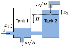
Figure 2. Two-tank system.

Define $\varphi(z)\coloneqq\Phi(z)-z$. Then the ODEs (61) can be rewritten in the form of Lur’e system (49) with

$$A\coloneqq\begin{bmatrix}-1&1\\ 1&-1\end{bmatrix},~{}~{}B\coloneqq\begin{bmatrix}1\\ 0\end{bmatrix},~{}~{}\xi\coloneqq\begin{bmatrix}1\\ -1\end{bmatrix},~{}~{}\eta\coloneqq\begin{bmatrix}-1\\ 1\end{bmatrix},$$

where the eigenvalues of $A$ are $0$ and $-2$. The feedback gain $K$ of the controller (50) is given by

$$K\coloneqq\begin{bmatrix}-0.7979&-0.6163\end{bmatrix},$$

which is the gain of the linear quadratic regulator with state weight $I$ and input weight $1$.

For simulations, we set $R_{0}\coloneqq 0.45$. Then the constants $\kappa_{\min}$ and $\kappa_{\max}$ in (51) are given by $\kappa_{\min}=-0.17$ and $\kappa_{\max}=0.35$. By solving the linear inequalities (53a) and (53b) with $c=0.4$, we obtain the vector $\theta_{\mathop{\textrm{cl}}\nolimits}=[1~{}~{}0.5180]^{\top}$ for the diagonally-weighted $\infty$-norm $\|\cdot\|_{\mathop{\textrm{cl}}\nolimits}=\|\cdot\|_{\infty,\theta_{\mathop{\textrm{cl}}\nolimits}}$. Similarly, we see that the vector $\theta_{\mathop{\textrm{op}}\nolimits}=[1~{}~{}1]^{\top}$ satisfies the linear inequalities (56a) and (56b) with $d_{1}=0$. Moreover, we have $R_{1}=0.1536$ by (55) and $R_{2}=0.225$ by (58). Using (57), we calculate the constant $d_{2}$ to be $2.8817$. From (59), we obtain $\Gamma=1.9305$. Then

$$R=\min\left\{R_{1},\frac{R_{2}}{\Gamma}\right\}=0.1166.$$

By (60), we set $\alpha=1.4142$. Note that the constant $\sigma_{0}\in\mathbb{R}_{>0}$ in Assumption 2.3 can be chosen arbitrarily. We summarize the parameters for Assumptions 2.1–2.3 in Table 1.

Remark 7.1.

If we set $\|\cdot\|_{\mathop{\textrm{op}}\nolimits}\coloneqq\|\cdot\|_{\mathop{\textrm{cl}}\nolimits}$, then $d_{1}\geq 1.2562$, which leads to smaller inter-sampling times; see the definitions (15) and (35) of $\psi_{\log}$ and $\psi_{\text{zo}}$. For this reason, we use different norms in Assumptions 2.1 and 2.2. $\triangle$

Table 1. Parameters for Assumptions 2.1–2.3.

Parameter	Value		Parameter	Value
$c$	$0.4$		$(d_{1},d_{2})$	$(0,2.8817)$
$\theta_{\mathop{\textrm{cl}}\nolimits}$	$[1~{}~{}0.5180]^{\top}$		$\theta_{\mathop{\textrm{op}}\nolimits}$	$[1~{}~{}1]^{\top}$
$R_{1}$	$0.1536$		$R_{2}$	$0.225$
$\Gamma$	$1.9305$		$R$	$0.1166$
$\alpha$	$1.4142$		$\sigma_{0}$	arbitrary

7.2. Simulation results of self-triggered control under logarithmic quantization

First we consider the STM (16) for logarithmic quantization. Fig. 3 shows the range of the threshold parameter $\sigma$ such that the condition (19) is satisfied for a given quantization density $\rho$. The blue and the red lines indicate the lower bound $\nicefrac{{\Gamma(1-\rho)}}{{(1+\rho)}}$ and the upper bound $\nicefrac{{2c\rho}}{{\alpha(1+\rho)}}$, respectively. When the pair $(\rho,\sigma)$ belongs to the gray region, then stabilization can be achieved by the STM (16). The upper and lower bounds intersect and take the value $0.2467$ at

$$\rho=\rho_{\min}\coloneqq 0.7734.$$

Therefore, when $\rho>\rho_{\min}$, the state trajectory starting in $\mathop{\mathbf{B}}_{\mathop{\textrm{cl}}\nolimits}\nolimits(R)$ exponentially converges without Zeno behavior for suitable $\sigma$ by Theorem 4.3. On the other hand, the upper bound $\nicefrac{{2c\rho}}{{\alpha(1+\rho)}}$ is $0.2828$ at $\rho=1$. Hence, when $\sigma\geq 0.2828$, the STM (16) does not guarantee the state convergence for any $\rho$.

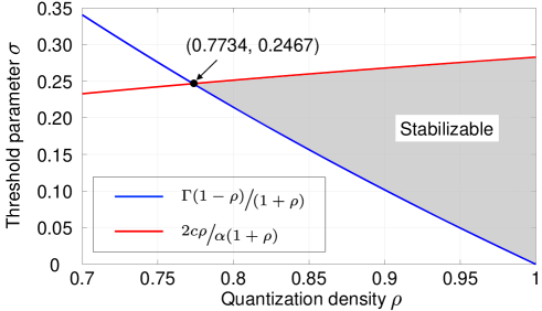
Figure 3. Stabilizable region of $(\rho,\sigma)$.

For simulations of time-responses, the parameters of logarithmic quantization are given by $\chi_{0}=R=0.1166$ and $\rho=0.85$. Then Assumption 4.1 is satisfied. The condition (19) on the threshold parameter $\sigma$ is written as

$$0.1565<\sigma<0.2599,$$

and we set $\sigma=0.25$. The upper bound $\tau_{\max}\in\mathbb{R}_{>0}$ of the inter-sampling times is arbitrary, and we set $\tau_{\max}=0.18$. We see from (20) that the inter-sampling times of the STM (16) are bounded from below by

$$\min\{\tau_{\min},\,\widetilde{\tau}_{\min}\}=\min\{0.0168,\,0.0281\}=0.0168,$$

where $\widetilde{\tau}_{\min}=0.0281$ is obtained by using the constant $\lambda=0.9251$ in Lemma 4.2. Table 2 summarizes the parameters used for the simulations in the logarithmic quantization case.

Table 2. Parameter settings for logarithmic quantization case.

Parameter	Value		Parameter	Value
$\chi_{0}$	$0.1166$		$\rho$	$0.85$
$\sigma$	$0.25$		$\tau_{\max}$	$0.18$

Figs. 4–6 show the time-responses with initial states $x_{1,0}=0.1$ and $x_{2,0}=-0.2$, where the time-step of the simulation is given by $10^{-5}$. We illustrate the state $x$ in Fig. 4, the input $u$ in Fig. 5, and the inter-sampling time $t_{k+1}-t_{k}$ in Fig. 6. The total number of sampling on the interval $(0,6]$ is $98$. In Fig. 4, the solid blue and red lines represent the states $x_{1}$ and $x_{2}$ of the quantized self-triggered control system, respectively. The dashed brawn and green lines are the time-responses of the states $x_{\text{ideal},1}$ and $x_{\text{ideal},2}$ of the ideal closed-loop system, where the input $u_{\text{ideal}}$ is given by $u_{\text{ideal}}=K[x_{\text{ideal},1}~{}~{}x_{\text{ideal},2}]^{\top}$. In Fig. 5, the solid blue and dashed red lines are the input $u$ of the quantized self-triggered control system and the input $u_{\text{ideal}}$ of the ideal closed-loop system, respectively.

From Fig. 4, we see that the state trajectory of the quantized self-triggered control system looks identical to that in the ideal closed-loop system. However, Fig. 5 shows that the input oscillates on the interval $[0,1]$ due to quantization. As shown in Fig. 6, the inter-sampling time is smaller on the same interval, because the state changes rapidly. We also observe that the inter-sampling time changes less frequently as the states converge.

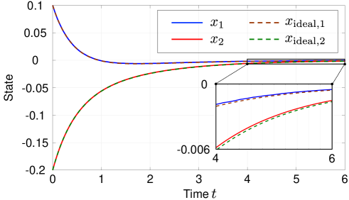
Figure 4. State under logarithmic quantization.

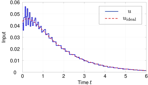
Figure 5. Input under logarithmic quantization.

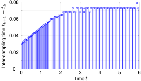
Figure 6. Inter-sampling times under logarithmic quantization.

7.3. Simulation results of self-triggered control under zooming quantization

Next we give simulation results in the case of zooming quantization. To the $i$-th state $x_{i}$, the function $Q$ applies uniform quantization with

$$\text{range $\left[-\dfrac{M}{\theta_{\mathop{\textrm{cl}}\nolimits,i}},\,\dfrac{M}{\theta_{\mathop{\textrm{cl}}\nolimits,i}}\right]$ $\quad$and$\quad$ step-size $\dfrac{2\Delta}{\theta_{\mathop{\textrm{op}}\nolimits,i}}$},$$

where $\theta_{\mathop{\textrm{cl}}\nolimits,i}$ and $\theta_{\mathop{\textrm{op}}\nolimits,i}$ are the $i$-th element of the weighting vectors $\theta_{\mathop{\textrm{cl}}\nolimits}$ and $\theta_{\mathop{\textrm{op}}\nolimits}$, respectively. The parameters of the zooming quantizer are given by $M=0.105$, $\Delta=5\times 10^{-3}$, and $\mu_{0}=1$. Then Assumption 5.1 is satisfied. The period $h$ for the STM (36) has to satisfy

$$0<h\leq\widetilde{\tau}_{\min}=5.7432\times 10^{-3},$$

where $\lambda=0.9837$ obtained from (32) is used for the computation of $\widetilde{\tau}_{\min}$. We set $h=10^{-3}$ for simulations. The upper bound $\ell_{\max}\in\mathbb{N}$ of $\ell_{k}$ is given by $\ell_{\max}=\nicefrac{{\tau_{\max}}}{{h}}=180$. The condition (38) with this period $h$ is written as

$$0.0533\leq\sigma<0.2828,$$

and we set $\sigma=0.075$. The parameters used for the simulations in the zooming quantization case are summarized in Table 3.

Note that the comparison between the threshold parameters $\sigma$ of the STMs (16) and (36) does not make sense. In fact, the threshold parameter is the coefficient of the quantized value $q_{k}$ in the logarithmic quantization case, while it is the coefficient of the quantization range $M\mu_{k}$ in the zooming quantization case. Moreover, a smaller $\sigma$ leads to a fast decay rate of the zoom parameter $\mu_{k}$ and hence quantization errors. Therefore, we choose the small threshold in the zooming quantization case.

Table 3. Parameter settings for zooming quantization case.

Parameter	Value		Parameter	Value
$M$	$0.105$		$\Delta$	$5\times 10^{-3}$
$\mu_{0}$	$1$		$h$	$10^{-3}$
$\ell_{\max}$	$180$		$\sigma$	$0.075$

Figs. 7–9 show the time-responses with initial states $x_{1,0}=0.1$ and $x_{2,0}=-0.2$, where the time-step of the simulation is given by $10^{-5}$. We illustrate the state $x$ in Fig. 7 and the input $u$ in Fig. 8, where each line represents the same as in Figs. 4 and 5. In addition, Fig. 9 shows the inter-sampling time $t_{k+1}-t_{k}$. The total number of sampling on the interval $(0,6]$ is $100$, which is closely aligns with the number of sampling, $98$, in the simulation of the logarithmic quantization case. From Figs. 7–9, we observe that the responses of the zooming quantization case have properties similar to those of the logarithmic quantization case. In fact, the state trajectories by quantized self-triggered control are quite close to those by the ideal control, but the input by quantized self-triggered control oscillates in the early response phase. Compared with the case of logarithmic quantization, the change of the input $u$ in Fig. 8 is still large on the interval $[4,6]$ due to coarse quantization. From Fig. 7, we observe that this leads to the oscillation of the state $x_{1}$ on the interval $[4,6]$. In Fig. 9, the inter-sampling time is smaller on the interval $[0,1]$ but larger on the interval $[2,6]$ than that in the logarithmic quantization case. This is because the STM (36) for zooming quantization uses the zoom parameter $\mu_{k}$ for the threshold. To avoid quantizer saturation, the update rule of $\mu_{k}$ is conservative. Namely, the decay rate of $\mu_{k}$ is smaller than that of $x$ in most cases. This makes the inter-sampling time on the interval $[2,6]$ larger than in the case of logarithmic quantization.

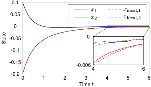
Figure 7. State under zooming quantization.

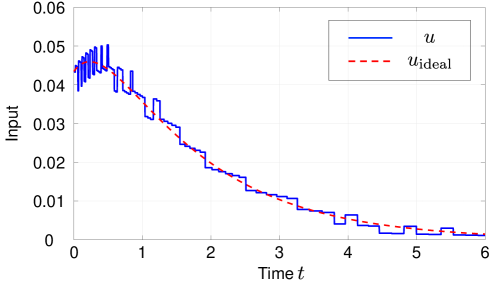
Figure 8. Input under zooming quantization.

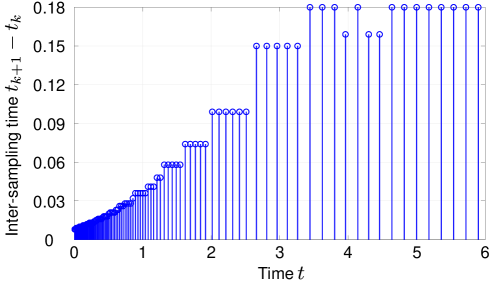
Figure 9. Inter-sampling times under zooming quantization.

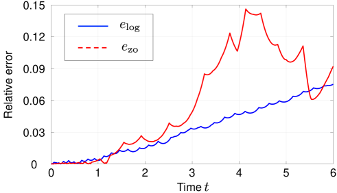
Figure 10. Comparison of relative errors.

7.4. Comparison of relative errors

In Fig. 10, we finally compare the relative errors of the states between the cases of logarithmic quantization and zooming quantization. Let $x_{\log,1}$ and $x_{\log,2}$ denote the states of the self-triggered control system under logarithmic quantization, whose parameters are as in Table 2. Then the relative error of the states under logarithmic quantization is defined by

$$e_{\log}(t)\coloneqq\frac{\sqrt{\sum_{i=1}^{2}|x_{\log,i}(t)-x_{\text{ideal},i}(t)|^{2}}}{\sqrt{\sum_{i=1}^{2}|x_{\text{ideal},i}(t)|^{2}}}$$

for $t\geq 0$. The relative error $e_{\text{zo}}(t)$ is defined in the same way for the states under zooming quantization, where the parameters are as in Table 3. From Fig. 10, we see that $e_{\log}$ grows linearly. In contrast, $e_{\text{zo}}$ increases rapidly on the interval $[3,4]$. Under logarithmic quantization, the quantization error is bounded by a constant multiple of the state norm; see the inequalities (11) and (12). On the other hand, the zoom parameter $\mu_{k}$ for zooming quantization decreases more slowly than the state, and as a result, the relative quantization error may increase exponentially. Thus, $e_{\text{zo}}$ has a growth behavior different from $e_{\log}$.

8. Conclusion

We studied the problem of stabilizing nonlinear systems under quantization and self-triggered sampling. In the closed-loop system we consider, only the quantized data of the state are available to the controller and the STM. The key assumption for stabilization is that the closed-loop system is contracting in the ideal case without quantization or self-triggered sampling. First, we presented a self-triggered control scheme that establishes, under logarithmic quantization, the exponential convergence of all state trajectories starting in a given region. Next, we proposed a joint strategy of zooming quantization and self-triggered sampling for stabilization. In both cases of logarithmic quantization and zooming quantization, the proposed STMs estimate the measurement error by predicting the state trajectory from the latest quantized state. We also discussed the assumptions of the proposed methods for the application to Lur’e systems.

There are still some open problems in quantized self-triggered control for nonlinear systems. Since the proposed STMs predict state trajectories based on the system model, the next sampling time cannot be computed correctly in the presence of disturbances and model uncertainty. Therefore, it would be beneficial to extend the techniques presented here to uncertain systems with disturbances. For applications to networked control systems, it is also important to explicitly address the robustness of the proposed control schemes with respect to transmission delays. Other topics for future work include cost-guaranteed control and output feedback stabilization.

.1. Proof of Lemma 4.4

To prove Lemma 4.4, we need a preliminary result.

Lemma A.

The function $W$ defined as in Lemma 4.4 is monotonically decreasing on $\mathbb{R}_{>0}$.

Proof.

Let $t\in\mathbb{R}_{>0}$. Then $w(t)>0$. Since

$$W^{\prime}(t)=\frac{1}{t^{2}}\left(-\frac{w^{\prime}(t)}{w(t)}t+\log w(t)\right),$$

it follows that

(62) $$W^{\prime}(t)<0\quad\Leftrightarrow\quad\Lambda(t):=-\frac{w^{\prime}(t)}{w(t)}t+\log w(t)<0.$$

Moreover,

$$\Lambda^{\prime}(t)=\frac{t\big{(}w^{\prime}(t)^{2}-w(t)w^{\prime\prime}(t)\big{)}}{w(t)^{2}},$$

and hence

(63) $$\Lambda^{\prime}(t)<0\quad\Leftrightarrow\quad w^{\prime}(t)^{2}-w(t)w^{\prime\prime}(t)<0.$$

We have

$$w^{\prime}(t)=-c(1-\varepsilon)e^{-ct}\quad\text{and}\quad w^{\prime\prime}(t)=c^{2}(1-\varepsilon)e^{-ct}.$$

From $0<\varepsilon<1$, we obtain

$$w^{\prime}(t)^{2}-w(t)w^{\prime\prime}(t)=-\varepsilon(1-\varepsilon)c^{2}e^{-2ct}<0,$$

and therefore $\Lambda^{\prime}(t)<0$ by (63). Since $w(0)=1$, we have $\Lambda(0)=0.$ This yields $\Lambda(t)<0$. Thus, $W$ is monotonically decreasing on $\mathbb{R}_{>0}$ by (62). ∎

Proof of Lemma 4.4: Since

$$w(t)<w(0)=(1-\varepsilon)+\varepsilon=1$$

for all $t\in\mathbb{R}_{>0}$, the definition of $W$ gives

$$\gamma=W(\tau_{\max})>0.$$

By Lemma A, $W(t)\geq W(\tau_{\max})$ for all $t\in[0,\tau_{\max}]$. This implies that

$$\frac{\log w(t)}{t}\leq-\gamma$$

for all $t\in[0,\tau_{\max}]$. Thus, desired inequality (22) holds. $\blacksquare$

References

- [1] M. Abdelrahim, V. S. Dolk, and W. P. M. H. Heemels. Event-triggered quantized control for input-to-state stabilization of linear systems with distributed output sensors. IEEE Trans. Automat. Control, 64:4952–4967, 2019.
- [2] A. Aghaeeyan and M. J. Yazdanpanah. Self-triggered impulsive control of nonlinear time delay systems: Application to chemotherapeutic dose-regimen design. Nonlinear Anal.: Hybrid Syst., 41:104047, 2021.
- [3] A. Anta and P Tabuada. To sample or not to sample: Self-triggered control for nonlinear systems. IEEE Trans. Automat. Control, 55:2030–2042, 2010.
- [4] A. Anta and P. Tabuada. Exploiting isochrony in self-triggered control. IEEE Trans. Automat. Control, 57:950–962, 2012.
- [5] M. D. Di Benedetto, S. Di Gennaro, and A. D’Innocenzo. Digital self-triggered robust control of nonlinear systems. Int. J. Control, 86:1664–1672, 2013.
- [6] R. W. Brockett and D. Liberzon. Quantized feedback stabilization of linear systems. IEEE Trans. Automat. Control, 45:1279–1289, 2000.
- [7] F. Bullo. Contraction Theory for Dynamical Systems. Kindle Direct Publishing, 1.1 edition, 2023.
- [8] A. Davydov, S. Jafarpour, and F. Bullo. Non-euclidean contraction theory for robust nonlinear stability. IEEE Trans. Automat. Control, 67:6667–6681, 2022.
- [9] A. Davydov, A. V. Proskurnikov, and F. Bullo. Non-euclidean contractivity of recurrent neural networks. In Proc. ACC’22, pages 1527–1534, 2022.
- [10] G. de Albuquerque Gleizer and M. Mazo. Self-triggered output-feedback control of LTI systems subject to disturbances and noise. Automatica, 120, Art. no. 109129, 2020.
- [11] G. Delimpaltadakis and M. Mazo. Isochronous partitions for region-based self-triggered control. IEEE Trans. Automat. Control, 66:1160–1173, 2021.
- [12] G. Delimpaltadakis and M. Mazo. Region-based self-triggered control for perturbed and uncertain nonlinear systems. IEEE Trans. Control Network Syst., 8:757–768, 2021.
- [13] D. Du, B. Qi, M. Fei, and Z. Wang. Quantized control of distributed event-triggered networked control systems with hybrid wired–wireless networks communication constraints. Inf. Sci., 380:74–91, 2017.
- [14] N. Elia and S. K. Mitter. Stabilization of linear systems with limited information. IEEE Trans. Automat. Control, 46:1384–1400, 2001.
- [15] A. Fu and J. Qiao. Periodic decentralized event-triggered control for nonlinear systems with asynchronous update and dynamic quantization. Nonlinear Dyn., 109:877–890, 2022.
- [16] M. Fu and L. Xie. The sector bound approach to quantized feedback control. IEEE Trans. Automat. Control, 50:1698–1711, 2005.
- [17] E. Garcia and P. J. Antsaklis. Model-based event-triggered control for systems with quantization and time-varying network delays. IEEE Trans. Automat. Control, 58:422–434, 2013.
- [18] T. Hayakawa, H. Ishii, and K. Tsumura. Adaptive quantized control for nonlinear uncertain systems. Syst. Control Lett., 58:625–632, 2009.
- [19] W. P. M. H. Heemels, J. Sandee, and P. van den Bosch. Analysis of event-driven controllers for linear systems. Int. J. Control, 81:571–590, 2008.
- [20] J. Heinonen. Lectures on analysis on metric spaces. New York: Springer, 2001.
- [21] M. Hertneck and F. Allogöwer. Dynamic self-triggered control fornonlinear systems based on hybrid Lyapunov functions. In Proc. 60th CDC, pages 533–539, 2021.
- [22] W. Kang, X.-N. Wang, and B.-Z. Guo. Observer-based fuzzy quantized control for a stochastic third-order parabolic PDE system. IEEE Trans. Syst., Man, Cybern., Syst., 53:485–494, 2023.
- [23] L. Li, X. Wang, and M. D. Lemmon. Efficiently attentive event-triggered systems with limited bandwidth. IEEE Trans. Automat. Control, 62:1491–1497, 2016.
- [24] D. Liberzon. Hybrid feedback stabilization of systems with quantized signals. Automatica, 39:1543–1554, 2003.
- [25] D. Liberzon. On stabilization of linear systems with limited information. IEEE Trans. Automat. Control, 48:304–307, 2003.
- [26] D. Liberzon. Finite data-rate feedback stabilization of switched and hybrid linear systems. Automatica, 50:409–420, 2014.
- [27] D. Liberzon and J. P. Hespanha. Stabilization of nonlinear systems with limited information feedback. IEEE Trans. Automat. Control, 50:910–915, 2005.
- [28] S. Liu, J. Cheng, D. Cao Zhang, H. J. Zhang, and A. Alsaedi. Dynamic quantized control for switched fuzzy singularly perturbation systems with event-triggered protocol. J. Frankl. Inst., 360:5996–6020, 2023.
- [29] T. Liu and Z.-P. Jiang. A small-gain approach to robust event-triggered control of nonlinear systems. IEEE Trans. Automat. Control, 60:2072–2085, 2015.
- [30] T. Liu and Z.-P Jiang. Event-triggered control of nonlinear systems with state quantization. IEEE Trans. Automat. Control, 64:797–803, 2018.
- [31] W. Liu, M. Wakaiki, J. Sun, G. Wang, and J. Chen. Self-triggered resilient stabilization of linear systems with quantized outputs. Automatica, 153:111006, 2023.
- [32] W. Lohmiller and J.-J. E. Slotine. On contraction analysis for non-linear systems. Automatica, 34:683–696, 1998.
- [33] M. Mazo, A. Anta, and P. Tabuada. An ISS self-triggered implementation of linear controllers. Automatica, 46:1310–1314, 2010.
- [34] G. N. Nair, F. Fagnani, S. Zampieri, and R. J. Evans. Feedback control under data rate constraints: An overview. Proc. IEEE, 95:108–137, 2007.
- [35] A. V. Proskurnikov and M. Mazo. Lyapunov event-triggered stabilization with a known convergence rate. IEEE Trans. Automat. Control, 65:507–521, 2020.
- [36] K.-E. Årzén. A simple event-based PID controller. In Proc. 14th IFAC World Congress, volume 18, pages 423–428, 1999.
- [37] K. J. Åström and B. M. Bernhardsson. Comparison of Riemann and Lebesgue sampling for first order stochastic systems. In Proc. 41st CDC, 2002.
- [38] A. Selivanov and E. Fridman. Distributed event-triggered control of diffusion semilinear PDEs. Automatica, 68:344–351, 2016.
- [39] Y. Shen, Z-G. Wu, P. Shi, Z. Shu, and H R. Karimi. control of Markov jump time-delay systems under asynchronous controller and quantizer. Automatica, 99:352–360, 2019.
- [40] P. Tabuada. Event-triggered real-time scheduling of stabilizing control tasks. IEEE Trans. Automat. Control, 52:1680–1685, 2007.
- [41] A. Tanwani, C. Prieur, and M. Fiacchini. Observer-based feedback stabilization of linear systems with event-triggered sampling and dynamic quantization. Systems Control Lett., 94:46–56, 2016.
- [42] D. Theodosis and D. V. Dimarogonas. Event-triggered control of nonlinear systems with updating threshold. IEEE Control Syst. Lett., 3:655–660, 2019.
- [43] U. Tiberi and K. H. Johansson. A simple self-triggered sampler for perturbed nonlinear systems. Nonlinear Anal.: Hybrid Syst., 10:126–140, 2013.
- [44] D. Tolić, R. G. Sanfelice, and R Fierro. Self-triggering in nonlinear systems: A small gain theorem approach. In Proc. 20th Mediterranean Conf. Control Automat., pages 941–947, 2012.
- [45] H. Tsukamoto, S.-J. Chung, and J.-J. E. Slotine. Contraction theory for nonlinear stability analysis and learning-based control: A tutorial overview. Annu. Rev. Control, 52:135–169, 2021.
- [46] M. Velasco, J. Fuertes, and P. Marti. The self triggered task model for real-time control systems. In Proc. 24th IEEE Real-Time Syst. Symp., pages 67–70, 2003.
- [47] M. Wakaiki. Self-triggered stabilization of discrete-time linear systems with quantized state measurements. IEEE Trans. Automat. Control, 68:1776 –1783, 2023.
- [48] M. Wakaiki and H. Sano. Event-triggered control of infinite-dimensional systems. SIAM J. Control Optim., 58:605–635, 2020.
- [49] M. Wakaiki and Y. Yamamoto. Stabilization of switched linear systems with quantized output and switching delays. IEEE Trans. Automat. Control, 62:2958–2964, 2017.
- [50] G. Wang. Event-triggered scheduling control for linear systems with quantization and time-delay. Eur. J. Control, 58:168–173, 2021.
- [51] X. Wang and M. D. Lemmon. Self-triggered feedback control systems with finite-gain stability. IEEE Trans. Automat. Control, 54:452–467, 2009.
- [52] T. Zhou, Z. Zuo, and Y. Wang. Self-triggered and event-triggered control for linear systems with quantization. IEEE Trans. Syst., Man, Cybern.: Syst., 50:3136–3144, 2018.