Coherent transient exciton transport in disordered polaritonic wires

Abstract

Excitation energy transport can be significantly enhanced by strong light-matter interactions. In the present work, we explore intriguing features of coherent transient exciton wave packet dynamics on a lossless disordered polaritonic wire. Our main results can be understood in terms of the effective exciton group velocity, a new quantity we obtain from the polariton dispersion. Under weak and moderate disorder, we find that the early wave packet spread velocity is controlled by the overlap of the initial exciton momentum distribution and its effective group velocity. Conversely, when disorder is stronger, the initial state is nearly irrelevant, and red-shifted cavities support excitons with greater mobility. Our findings provide guiding principles for optimizing ultrafast coherent exciton transport based on the magnitude of disorder and the polariton dispersion. The presented perspectives may be valuable for understanding and designing new polaritonic platforms for enhanced exciton energy transport.

Emory University] Department of Chemistry and Cherry Emerson Center for Scientific Computation, Emory University, Atlanta, Georgia, United States of America

Introduction

The strong light-matter interaction regime is achieved when the coupling strength between light and matter overcomes dephasing and dissipative phenomena acting on each subsystem. This can be accomplished, for example, with a molecular ensemble with a narrow linewidth bright transition near resonance with an optical microcavity composed of two parallel mirrors with high-reflectivity^{1, 2, 3}. In this scenario, the field confinement and low mode volumes allow light and matter to exchange energy (quasi)reversibly. Several recent studies have shown that strong light-matter coupling can be harnessed to control energy ^{4, 5, 6, 7, 8, 9, 10, 11, 12, 13, 14, 15, 16, 17, 18} and charge^{19, 20, 21, 22, 23} transport in disordered materials. These effects are attributed to the formation of polaritons, i.e., hybrid light-matter states with intermediate properties between purely material or photonic. For example, polariton delocalization ^{24, 25, 26, 27} is often invoked to explain the properties of energy transport in the strong coupling regime³.

Unlike bare excitons, which tend to show weak delocalization and inefficient energy transfer in disordered media, polaritons show much greater diversity in wave function delocalization ^{24, 28, 29, 30, 31} and transport phenomena ^{9, 16, 18}. For instance, polariton transport imaging has revealed ultrafast ballistic propagation in perovskite microcavities¹⁶ and surface-bound polaritons^{11, 18}, with spread velocities spanning several orders of magnitude. The effects of disorder on polariton transport have also received significant attention as the potential source of the slower-than-expected polariton wave packet propagation reported by several groups ^{15, 18, 16}. Indeed, theoretical investigations suggest that dynamic and static disorder inhibit polariton wave packet propagation by effectively reducing the propagation velocity ^{16, 32, 33}. Interestingly, recent theoretical investigations of dipolar exciton propagation in finite one-dimensional systems suggest that under strong disorder, a disorder-enhanced transport regime emerges where coherent exciton propagation benefits from an increase in the static fluctuations of matter excitation energies ^{34, 33, 31}.

Our recent work on coherent transport in polaritonic wires ³³ thoroughly examined the requirements for convergence of exciton transport simulations with respect to model parameters, showed multiple (on and off-resonant) electromagnetic mode ³³ played a key role in the exciton dynamics, and demonstrated the potential to control transient ballistic and diffusive exciton transport and Anderson localization under strong light-matter coupling. Here, we focus on the transient early dynamics of exciton wave packets propagating on a lossless polaritonic wire. In particular, we present numerical simulations and a detailed theoretical analysis of coherent polariton-mediated exciton transport in the ballistic regime. Our results and mathematical analysis reveal several surprising aspects of polariton-assisted coherent exciton transport, including a striking difference between the effect of disorder on ultrafast coherent exciton propagation in free space ³⁵ and in a polaritonic medium and the notion that an effective exciton group velocity may be defined that allows a qualitative understanding of our numerical simulations even in a moderately disordered scenario.

This article is organized as follows: in Section 2, we describe the theory and method employed in this work. Section 3 contains our main numerical results and theoretical analysis, while Section 4 provides conclusions and a summary of this work.

Theory and Computation

The polaritonic wire model employed here consists of a linear chain of dipoles representing matter (e.g., atoms, quantum wells, or molecules with negligible vibronic coupling) coupled to photon modes of a lossless cuboid optical microcavity of lengths $L_{x}$, $L_{y}$, and $L_{z}$ as depicted in Fig. 1. Each dipole is a two-level system with excitation energy given by $\hat{H}_{M}|n;0\rangle=E_{n}|n;0\rangle$, where $|n;0\rangle$ represents a state where the $n$-th dipole is in its excited state, while all other dipoles and cavity modes are in their ground states. The excitation energy of each dipole $E_{n}$ is sampled from a normal distribution with average $E_{M}$ and standard deviation $\sigma_{M}$. Different detuning and static disorder strengths are accessed by adjusting these parameters. The spatial distribution of dipoles is also sampled from a normal distribution, but in this case, the average and standard deviation are fixed at 10 and 1 nm, respectively. The large intersite separation allows us to disregard direct interaction between these dipoles since direct energy transfer via FRET would occur at a much larger times scale than probed here. Furthermore, we also impose the same orientation for all dipoles, such that they can only interact with transverse electric (TE) polarized photon modes, and we need not consider the transverse magnetic polarization.

Imposing vanishing electric field along the $y$ and $z$ directions and periodic boundary conditions along the long-axis $x$ implies

$$\mathbf{k}=\left(\frac{2\pi m_{x}}{L_{x}},\;\frac{\pi n_{y}}{L_{y}},\;\frac{\pi n_{z}}{L_{z}}\right)\,,$$ (1)

where $m_{x}\in\mathbb{Z}$ and $n_{y},n_{z}\in\mathbb{N}_{>0}$. Throughout this work, we employ a geometry where $L_{x}=50$ $\mu m$, $L_{y}=0.2$ $\mu m$, and $L_{z}=0.4$ $\mu m$, such that the energy gap between adjacent bands is large ($>0.5$ eV) enough that we restrict our analysis to the lowest energy band ($n_{y}=1$ and $n_{x}=1$). By defining $q=k_{x}=\frac{2\pi m_{x}}{L_{x}}$ and $q_{0}=\sqrt{k_{x}^{2}+k_{y}^{2}}=\sqrt{\left(\frac{\pi}{L_{x}}\right)^{2}+\left(\frac{\pi}{L_{y}}\right)^{2}}$, it follows we can uniquely identify each photon mode using its value of $q$. The energy of each mode is

$$\hbar\omega_{q}=\frac{\hbar c}{\sqrt{\epsilon}}\sqrt{q^{2}+q_{0}^{2}}\,,$$ (2)

where $\hbar$ is the reduced Planck constant, $c$ is the speed of light, and $\epsilon$ is the relative permittivity of the intracavity medium. We use $\epsilon=3$ as a suitable parameter for organic microcavities. From Eq. 2, the minimum photon energy supported in the cavity is $\hbar cq_{0}/\sqrt{\epsilon}=2.00$ eV.

The non-interacting part of the light-matter Hamiltonian is

$$\hat{H}_{0}=\sum_{n}E_{n}\hat{b}^{\dagger}_{n}\hat{b}_{n}+\sum_{q}\hbar\omega_{q}\hat{a}^{\dagger}_{q}\hat{a}_{q}\,,$$ (3)

where $\hat{b}^{\dagger}_{n}$ and $\hat{a}^{\dagger}_{n}$ are ladder operators creating a dipolar excitation at the $n$-th site and a photon in the $q$ mode, respectively. We employ the Coulomb gauge in the rotating wave approximation while neglecting the diamagnetic contribution. It follows the interacting part of the Hamiltonian can be expressed as

$$\hat{H}_{\text{int}}=\sum_{n=1}^{N_{M}}\sum_{q}\frac{-i\Omega_{R}}{2}\sqrt{\frac{E_{n}}{N_{M}\hbar\omega_{q}}}\left(e^{iqx_{n}}\hat{b}_{n}^{\dagger}\hat{a}_{q}-e^{-iqx_{n}}\hat{a}_{q}^{\dagger}\hat{b}_{n}\right)\,,$$ (4)

where $N_{M}$ is the total number of sites and $x_{n}$ is the position of the $n$-th dipole along $x$. The parameter $\Omega_{R}$ (Rabi splitting) is related to the transition dipole moment of each molecule ($\vec{\mu_{d}}$) by

$$\Omega_{R}=\vec{\mu_{d}}\cdot\hat{\mathbf{z}}\sqrt{\frac{\hbar\omega_{0}N_{M}}{2\epsilon L_{x}L_{y}L_{z}}}\,.$$ (5)

To make our study computationally tractable, we truncate the model in the number of molecules and photon modes. Following the thorough analysis in our previous work ³³, we set $N_{M}=5000$ to minimize finite-size effects in the sub-picosecond region. Similarly, we include 1001 cavity modes ($-500\leq m_{x}\leq 500$), which span an energy range of 7.43 eV, well above the necessary for convergent results.

In all simulations presented here, the initial state is a Gaussian exciton wave packet with zero photonic content. This initial state can be represented in the uncoupled basis as

$$\ket{\psi(0)}=\frac{1}{Z}\sum_{n}\exp\left[-\frac{(x_{n}-\frac{1}{2}L_{x})^{2}}{4\sigma_{x}^{2}}+i\bar{q}_{0}x_{n}\right]\ket{n;0}\,,$$ (6)

where $Z$ is a normalization constant, $\sigma_{x}$ is the initial spread of the wave packet, and $\bar{q}_{0}$ is the average exciton momentum along $x$. From now on, we set $\bar{q}_{0}=0$ unless otherwise noted. Note that $\sigma_{x}$ is the standard deviation of the probability distribution $P(n)=|\innerproduct{n;0}{\psi(0)}|^{2}$. The reciprocal space distribution $P(q)$, obtained from the Fourier change of basis in (6), has standard deviation $\sigma_{q}$ related to $\sigma_{x}$ via

$$\sigma_{x}\sigma_{q}=\frac{1}{2}\;.$$ (7)

In all simulations, the Fock space is truncated to include only states with one excited dipole and no photons ($\ket{n;0}$) or one photon and no dipolar excitations ($\ket{0;q}$). The dynamics generated by $\hat{H}=\hat{H}_{0}+\hat{H}_{\text{int}}$ and the initial state $\ket{\psi(0)}$ is in fact constrained to the single excitation subspace. Thus, our results are relevant to coherent dipolar dynamics when nonlinearities can be ignored (e.g., due to a small density of excitons). The time-evolved wave packet is directly obtained from $\ket{\psi(t)}=e^{-i\hat{H}t/\hbar}\ket{\psi(0)}$ using the eigenvalues and eigenvectors of $\hat{H}$ within the one-excitation manifold ($\ket{n;0}\oplus\ket{0;q}$).

Our computational study follows the transient evolution of exciton wave packets starting from the well-localized purely excitonic state in Eq. 6. As a metric for the exciton spread, we compute the root mean square displacement of the dipolar component of the wave packet, defined here as

$$\text{RMSD}(t) =\left[\frac{1}{P_{\text{M}}(t)}\sum_{n=1}^{N_{M}}|\bra{n;0}\ket{\psi(t)}|^{2}(x_{n}-x_{0})^{2}\right]^{1/2}\,,$$ (8)

$$P_{\text{M}}(t) =\sum_{n}^{N_{M}}|\bra{n;0}\ket{\psi(t)}|^{2}\,.$$ (9)

where the renormalization factor $P_{M}(t)$ is the time-dependent probability of finding any excited dipole and $x_{0}$ is the average exciton position at $t=0$ (which in this work is always $\frac{L_{x}}{2}=25\;\mu$m). As an alternative and complementary metric of exciton mobility, we define the (matter normalized) migration probability $\chi(t)$, which measures the conditional probability of finding an excited dipole outside the region where the wave packet was initially localized. By choosing symmetric boundaries $n_{\text{min}}\leq n\leq n_{\text{max}}$ such that there is at least 99% chance ($\frac{L_{x}}{2}-3\sigma_{x}<x<\frac{L_{x}}{2}+3\sigma_{x}$) that the exciton at time $t=0$ lies within this region, we compute the migration probability as

$$\chi(t)=1-\frac{1}{P_{\text{M}}(t)}\sum_{n=n_{\text{min}}}^{n_{\text{max}}}|\bra{n;0}\ket{\psi(t)}|^{2}\,.$$ (10)

The code used in all simulations is available in our prototype package PolaritonicSystems.jl ³⁶. Random variables were generated using the Distributions.jl package³⁷ and the Makie.jl plotting ecosystem ³⁸ was used for data visualization.

Figure 1: Illustration of the polariton wire model. Dipoles representing matter are non-interacting two-level systems aligned with the z-axis. Distances between sites are sampled from a normal distribution with an average and standard deviation of 10 and 1 nm, respectively. Likewise, excitation energies for each dipole are sampled from a normal distribution using an average of $E_{M}$ and standard deviation of $\sigma_{M}$. These parameters control the detuning and static disorder of the system. Radiation states inside the cavity are constructed using 1001 modes of the lowest energy band, with a minimum photon energy of 2.00 eV.

Results and Discussion

Polariton-mediated exciton wave packet propagation

Selected wave packet snapshots are given in Fig. 2, along with the corresponding time-dependent exciton RMSD, $P_{M}$, and migration probability $\chi$. The main effect of static disorder can be observed in these examples. From Figs. 2a to c, as disorder is increased, the wave packet mobility is significantly reduced, and its spread is strongly suppressed. Simultaneously, we find the photonic content and its time-dependent fluctuations monotonically decrease and become small under strong disorder (e.g., $P_{M}(t)$ is relatively stable around 0.97 when $\sigma_{M}/\Omega_{R}=100\%$). In contrast, photon content fluctuations are large under weak disorder ($\sigma_{M}/\Omega_{R}\rightarrow 0$). The effect of disorder on photon content fluctuations may be directly understood from Rabi oscillations which occur unperturbed at weak disorder while being strongly damped as $\sigma_{M}$ approaches $\Omega_{R}$ ³³. These observations illustrate how the oscillatory energy exchange between radiation and matter leads to enhanced coherent exciton transport.

Figure 2: Average exciton wave packet profiles at different time delays and relative disorder strength ($\sigma_{M}/\Omega_{R}$) of 5%, 20%, and 100% for (a), (b) and (c), respectively. In all cases, $\Omega_{R}=0.1$ eV and the wave packet initial width and mean quasimomentum are $\sigma_{x}=120$ nm and $\bar{q}_{0}=0$. Probabilities are grouped in bins containing 50 dipoles spanning 0.5 $\mu m$. $P_{M}$, RMSD, and $\chi$ are defined in Eqs. 8,9, and 10, respectively. Each profile is obtained from the average of 100 disorder realizations.

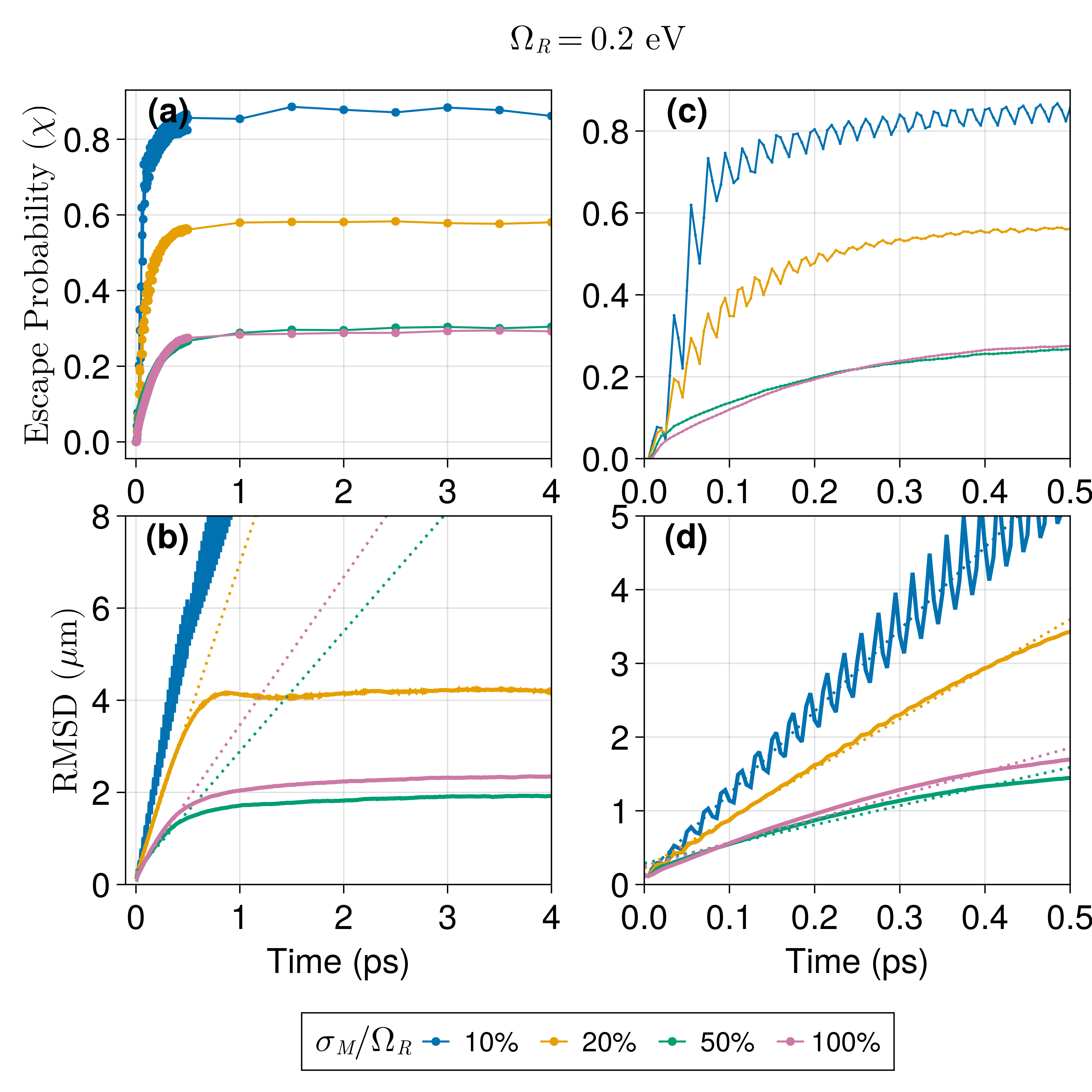
Figure S6: Propagation of exciton wave packets at different disorder strengths measured by (a) escape probability (Eq. 10) and (b) RMSD (Eq. 8). In all cases, $\sigma_{x}=120$ nm and $\Omega_{R}=0.2$ eV. Results are averages of 100 disordered realizations. The dotted lines in (b) are linear fits on the early propagation ($\leq$ 500 fs) from which slopes are used to measure the initial ballistic velocity ($v_{0}$). Panels (c) and (d) are zoomed in versions of (a) and (b), respectively.

In Fig. 3, the average exciton migration probability (Equation 10) and RMSD are shown for excitons propagating over 4 ps under different values of relative disorder strength ($\sigma_{M}/\Omega_{R}$). The migration probability, seen in Fig. 3a, increases rapidly before achieving a steady state ($\mathrm{d}\chi(t)/\mathrm{d}t\approx 0$) around 2 ps irrespective of the disorder strength. Conversely, disorder plays a crucial role in the sub-300 fs phase of the dynamics, where we find from the inset that in all considered cases, an increase in $\sigma_{M}$ leads to a slower initial exciton migration. From the behavior of $\chi(t)$ at large $t$, we find the steady-state exciton migration probability at weak disorder is largely suppressed when $\sigma_{M}$ is increased. Nevertheless, the strongly disordered cases ($\sigma_{M}/\Omega_{R}\geq 1$) suggest that beyond a particular disorder strength, $\chi(t\gg 0)$ becomes approximately independent of $\sigma_{M}$. Figs. S6 and S7 provide $\chi(t)$ for $\Omega_{R}=0.2$ eV and $\Omega_{R}=0.3$ eV under different levels of disorder and verify the disorder effects on $\chi(t)$ described above are in fact generic.

In the SI Section 2, we show the initial growth of $\chi(t)$ can be approximated in the weak and strong disorder limits by analyzing the disorder-averaged properties of $|\innerproduct{0;n}{\psi(t)}|^{2}$. This leads to the conclusion that $\partial\chi(t)/\partial t\rightarrow 0$ as $t\rightarrow 0^{+}$, so that the quantity $G=(1/2)\partial^{2}\chi(t)/\partial t^{2},~{}t\rightarrow 0^{+}$ controls the early growth of $\chi(t)$. In the weak and strong disorder limits, $G$ satisfies, respectively

$$G^{W}\approx\frac{1}{2N_{\mathcal{I}}}\sum_{A,B\neq A}\sum_{n\in\mathcal{I}}|A_{n}|^{2}|B_{n}|^{2}(\omega_{A}-\omega_{B})^{2},$$ (11)

$$G^{S}\approx\frac{1}{2}\sum_{A,B\neq A}\sum_{n\in\mathcal{I}}\overline{|A_{n}|^{2}|B_{n}|^{2}}|c_{n}|^{2}(\omega_{A}-\omega_{B})^{2},$$ (12)

where $A$ and $B$ are eigenstates, $A_{n}$ and $B_{n}$ the probability amplitude to detect an exciton at the $n$th dipole when the system is in the $A$ and $B$ eigenstates, respectively, $\mathcal{I}=[n_{\text{min}},n_{\text{max}}]$ (see Eq. 10 and accompanying description), $N_{\mathcal{I}}$ is the number of sites in $\mathcal{I}$, and $\overline{f}$ implies that we are taking the disorder average of quantity $f$. From these approximations to $G$, the ultrafast increase in the exciton migration probability depends on the existence of eigenstates with large energy differences and significant contributions from the dipoles comprising the initial wave packet.

From Eq. 12, we infer (i) the steep increase of $\chi(t)$ at early times monotonically increases with $\Omega_{R}$ at fixed energetic disorder (as the energy difference between polariton modes formed from near-resonant photon and excitons increase with $\Omega_{R}$), (ii) increasing disorder with fixed $\Omega_{R}$ leads to initial slower growth of $\chi\left(t\rightarrow 0^{+}\right)$, due to the greater tendency of localization of the $n$-th exciton into a strongly localized eigenmode. Importantly, while the summand of Eq. (11) has the same form as that of Eq. 12, the former has several more contributions than the latter ($N_{\mathcal{I}}^{2}$ in the approximation given in Eq. 11), and therefore, a much steeper early increase occurs in $\chi(t)$ under weak disorder.

In summary, as measured by $\chi(t)$, indeed, disorder slows down the ability of excitons to migrate at very early times, and increasing the Rabi splitting leads to faster initial migration probability for dipoles in photonic wires. Similar considerations can be made on the asymptotic ($t\rightarrow\infty)$ behavior of $\chi(t)$: disorder averaging and the lack of correlation between the excitation energy at distinct sites suppresses cross-terms in the strong disorder limit relative to weak, and therefore, a reduced $\sigma_{M}$ favors a larger steady-state value of $\chi(t)$.

The RMSD measure reported in Fig. 3b, also indicates the excitonic propagation is fastest in the fs time scale. Both $\chi(t\rightarrow\infty)$ and RMSD($t\rightarrow\infty$) drop when the $\sigma_{M}/\Omega_{R}$ is increased from 20% to 40%. However, comparing the 80% and 100% relative disorder strength cases in Fig. 3b, we note the emergence of a disorder-enhanced transport regime (DET) as reported in previous studies of dipole chains under strong light-matter interactions ^{39, 34, 33, 31}. This DET regime clearly leaves no signature in $\chi(t)$ (Fig. 3a), but may be understood based on earlier studies of exciton transport in a polaritonic wire ^{34, 31}. Specifically, in this regime, weakly coupled excitons are exponentially localized, albeit with extended tails. Due to their small associated probabilities, these tails are inconsequential for the exciton migration probability. Still, they provide sizable contributions to the RMSD due to their large extent relative to $\sigma_{x}$ (see SI Figs. S1-S3 and accompanying text for additional discussion).

In Fig.3b, dotted lines represent linear fits obtained from the first 500 fs of simulation. This initial linear behavior (minimum coefficient of determination $R^{2}=0.98$) characterizes the excitonic ballistic spread. In the next sections, we will use this value as a measure of the initial exciton spread velocity ($v_{0}$).

To conclude this subsection, we note the polariton-mediated ultrafast exciton transport described here shows intriguing differences relative to bare exciton transport analyzed in a recent study by Cui et al. ³⁵. Their work showed that transient ultrafast energy transfer mediated by direct short-range interactions benefits from the existence of static disorder, leading to faster transport (relative to a perfectly ordered system) in the femtosecond timescale. Cui et al. ascribe their observation of transient disorder enhancement of transport to the suppression of destructive interference induced by the heterogeneity of the matter excitation energies ³⁵. Here, we find the opposite feature: disorder always reduces the initial transport velocity. Even in the DET regime, Fig.3b shows a narrow window at early times where transport is subdiffusive ³³. This contrast points towards a fundamental difference in how static disorder affects direct (purely) excitonic and polariton-mediated coherent energy transport.

Figure 3: Propagation of exciton wave packets at different disorder strengths measured by (a) migration probability (Eq. 10) and (b) RMSD (Eq. 8). In all cases, $\sigma_{x}=120$ nm and $\Omega_{R}=0.1$ eV. Results are averages of 100 disordered realizations. The dotted lines in (b) are linear fits of the early propagation ($\leq$ 500 fs) from which slopes are used to measure the initial ballistic velocity ($v_{0}$). Insets show a zoomed-in view into the sub 500 fs region.

Ballistic Exciton Transport

In Fig. 4, the initial exciton spread velocity ($v_{0}$) is shown as a function of relative disorder $\sigma_{M}/\Omega_{R}$. We examine $v_{0}$ obtained for systems with variable collective light-matter interaction strength $\Omega_{R}$ (with fixed relative disorder $\sigma_{M}/\Omega_{R}$) and two selected initial wave packet sizes ($\sigma_{x}$ in Eq. 6). In both cases, we observe an initial steep decay of $v_{0}$ with increasing $\sigma_{M}/\Omega_{R}$ which is followed by a plateau until the DET regime is reached at $\sigma_{M}/\Omega_{R}\approx 1$. However, a salient difference in the variation of $v_{0}$ with $\Omega_{R}$ at low disorder is observed between the narrow ($\sigma_{x}=120$ nm) and the broader ($\sigma_{x}=480$ nm) wave packets in Figs. 5a and b, respectively. This difference vanishes quickly when disorder is increased, demonstrating the initial state preparation is less important to the dynamics under strong disorder. Nevertheless, the distinct $\Omega_{R}$ dependence of $v_{0}$ is observable in a sizable range of disorder strengths (0$\sim$30%), thereby warranting a mechanistic explanation. We pursue that by analyzing below the (excitonic) spread velocity of the wave packet in the absence of disorder.

The detailed mathematical treatment of the spread velocity, which we summarize below, is provided in Section 1 of the SI. We first emphasize that the treatment of the ballistic transport regime is unconventional even in the zero-disorder case because (a) our initial wave packets range from strongly localized ($\sigma_{x}=120~{}\text{nm})$ to moderately delocalized $(\sigma_{x}=480~{}\text{nm})$ in real space, (b) the wave packet has LP and UP components, and (c) the polariton dispersion is not quadratic. These features imply the basic treatment of Gaussian wave packet transport in a quadratic medium, generally valid for sufficiently narrow wave packets in $q$-space, is inapplicable ⁴⁰. With these considerations, we show (see SI) that the dominant contribution to the exciton transport velocity $v_{0}$ is given by

$${v}^{2}_{0}\approx\sum_{q}P(q)\left[\left(v_{\text{LP}q}^{\text{eff}}\right)^{2}+\left(v_{\text{UP}q}^{\text{eff}}\right)^{2}\right]\;,$$ (13)

where $P(q)$ is the $t=0$ exciton probability distribution in $q$-space. From Eq. 7, the width $\sigma_{q}$ of $P(q)$ is inversely proportional to the real-space width of the initial wave packet $\sigma_{x}$. The effective group velocity $v_{\alpha q}^{\text{eff}}$ (where $\alpha$ is UP or LP) is defined as

$$v_{\alpha q}^{\text{eff}}=\Pi_{\alpha q}v_{g}^{\alpha q}=\Pi_{\alpha q}\frac{\partial\omega_{\alpha q}}{\partial q}\;,$$ (14)

where $\Pi_{\alpha q}$ is the total exciton content of the polariton mode $\alpha$ with wave number $q$, and $\frac{\partial\omega_{\alpha q}}{\partial q}$ is the (conventional) group velocity $v_{g}^{\alpha q}$ of the same mode. The polaritonic group velocity weighted by the corresponding exciton content $\Pi_{\alpha q}$ yields the effective exciton group velocity $v_{\alpha q}^{\text{eff}}$ of mode $\ket{\alpha q}$. The total matter content $\Pi_{\alpha q}$ plays a key role because even though high energy regions of the UP branch yield the largest $v_{g}^{\alpha q}$, their small $\Pi_{\alpha q}$ results in negligible $v_{\alpha q}^{\text{eff}}$ values. From Eq. 13 one can see that $v_{0}$ is controlled by the effective group velocity $v_{\alpha q}^{\text{eff}}$ weighted by the exciton $P(q)$ distribution. Hence, as we demonstrate below, the different ways $P(q)$ and $v_{\alpha q}^{\text{eff}}$ overlap explain the varying mobility of differently prepared excitons in weakly and moderately disordered systems.

Effective group velocities $v_{\alpha q}^{\text{eff}}$ for systems with $\Omega_{R}=0.1$ and $\Omega_{R}=0.2$ eV are presented with an overlay of $P(q)$ for several initial exciton wave packets in Fig. 5. The first relevant observation is the substantial increase of $v_{\alpha q}^{\text{eff}}$ with $\Omega_{R}$ for both $\alpha=\text{LP}$ and UP with $q>0.003$ nm^-1. The Rabi splitting does not affect the effective group velocity for polariton modes with $q<0.003$ nm^-1. This feature explains the Rabi splitting dependence of $v_{0}$ observed in Fig. 4b in weakly and moderately disordered systems. Specifically, a broad wave packet in real space (e.g., $\sigma_{x}=480$ nm) is narrow in $q$-space and does not vanish at a small interval of $q$ near zero (the wave packet center in $q$ space) where $v_{\alpha q}^{\text{eff}}$ is nearly identical for all values of $\Omega_{R}$ examined here. Therefore, as seen in Fig. 4b, sufficiently broad wave packets show no significant dependence on $\Omega_{R}$ when $\sigma_{M}/\Omega_{R}$ is not too large (up to 40$\%$ in Fig. 4).

Figure 4: Initial spread velocity ($v_{0}$) for various systems at different relative disorder strength and Rabi splitting values for wave packets with a (a) narrow and b broad initial spread values ($\sigma_{x}$, see Eq. 6). Each point is the average of 100 disordered realizations. $v_{0}$ was computed as the slope of a linear fit of RMSD values in the initial 500 fs of simulation (see Fig. 3).

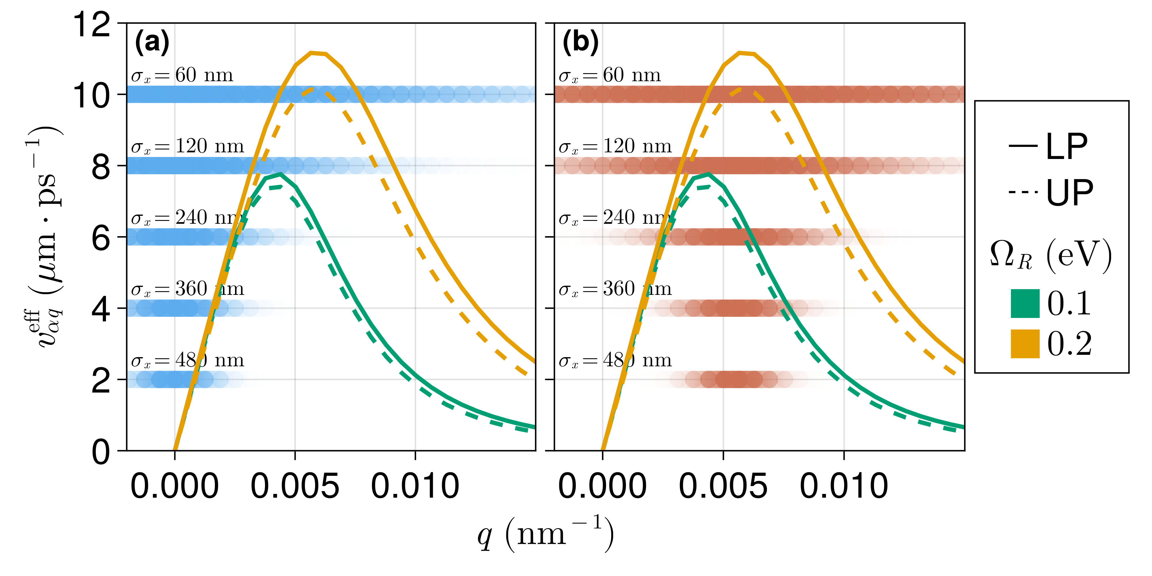
Figure 5: Effective group velocity (Eq. 14) for different values of $\Omega_{R}$. Horizontal gradient bars represent the $P(q)$ distribution for different exciton wave packets (see Eq. 6) with (a) $\bar{q}_{0}=0.0$ and (b) $\bar{q}_{0}=0.0055$ nm^-1. The overlap between the gradient bars ($P(q)$) and the $v_{\alpha q}^{\text{eff}}$ curves yields the exciton spread velocity $v_{0}$ (Eq. 13). See text for more details.

In Fig. 6, we present quantitative evidence that Eqs. 13 and 14 appropriately describe the early-time exciton wave packet propagation rate under small and moderate disorder conditions. In particular, Fig. 6 shows $v_{0}$ vs. $\sigma_{x}$ at various relative disorder strengths ($\sigma_{M}/\Omega_{R}$). As shown in Fig. 6a, in almost every case considered, when the initial state has zero average momentum ($\bar{q}_{0}=0$), an increase in $\sigma_{x}$ results in a slower propagation. This generic behavior at weak and moderate disorder can be readily understood from Figs. 5a and b. As $\sigma_{x}$ broadens, the width of the $P(q)$ distribution (centered at $\bar{q}_{0}=0$) is reduced, and $v_{0}$ decreases due to the increasing dominance of contributions with small effective group velocities in Eq. 13.

The gray dotted curves in Fig. 6 follow from Eq. 13. This Equation not only captures the overall qualitative trend at small and moderate disorder, but it also reproduces the local maximum at $\sigma_{x}=120$ nm in Fig. 6a. This peak can be explained again based on Fig. 5: by increasing the wave packet width in $q$-space, polariton components with larger $v_{\alpha q}^{\text{eff}}$ become relevant and $v_{0}$ (Eq. 13) increases, but if $P(q)$ becomes too broad (e.g., $\sigma_{x}=60$ nm), polaritons with smaller $v_{\alpha q}^{\text{eff}}$ (with $q$ greater than the maxima in $v_{\alpha q}^{\text{eff}}$) start to contribute significantly to $v_{0}$ (at the expense of high exciton group velocity components) leading to an overall reduction in the magnitude of $v_{0}$.

Fig. 6b shows analogous results for an exciton prepared with $\bar{q}_{0}=0.005654$ nm^-1. Indeed, in this case, broader wave packets display higher mobility as measured by $v_{0}$. This is expected based on Eqs. 13 and 14 as here a smaller uncertainty in $q$ (increased $\sigma_{x}$) localizes $P(q)$ around $q\approx\bar{q}_{0}\neq 0$ where the corresponding $v_{\alpha q}^{\text{eff}}$ values are non-zero (see Fig. 5b). Overall, these results give a simple prescription to optimize polariton-mediated coherent exciton transport by preparing a sufficiently broad initial state with (mean)effective group velocity at the maximum of $v_{\alpha q}$.

Note that polariton states no longer have well-defined $q$ values in the presence of nonvanishing disorder, and strictly speaking, the arguments above based on uncertainty relations break down. However, as shown in Fig. 6, this breakdown is only observed when $\sigma_{M}/\Omega_{R}=1.0$, where $v_{0}$ is nearly independent of $\sigma_{x}$. Our analysis (in terms of uncertainty relations and Eqs. 13 and 14) is seen to hold qualitatively for $\sigma_{M}/\Omega_{R}<40\%$, indicating the here employed arguments are generally applicable for examination of coherent exciton transport at early times even in systems with moderate disorder.

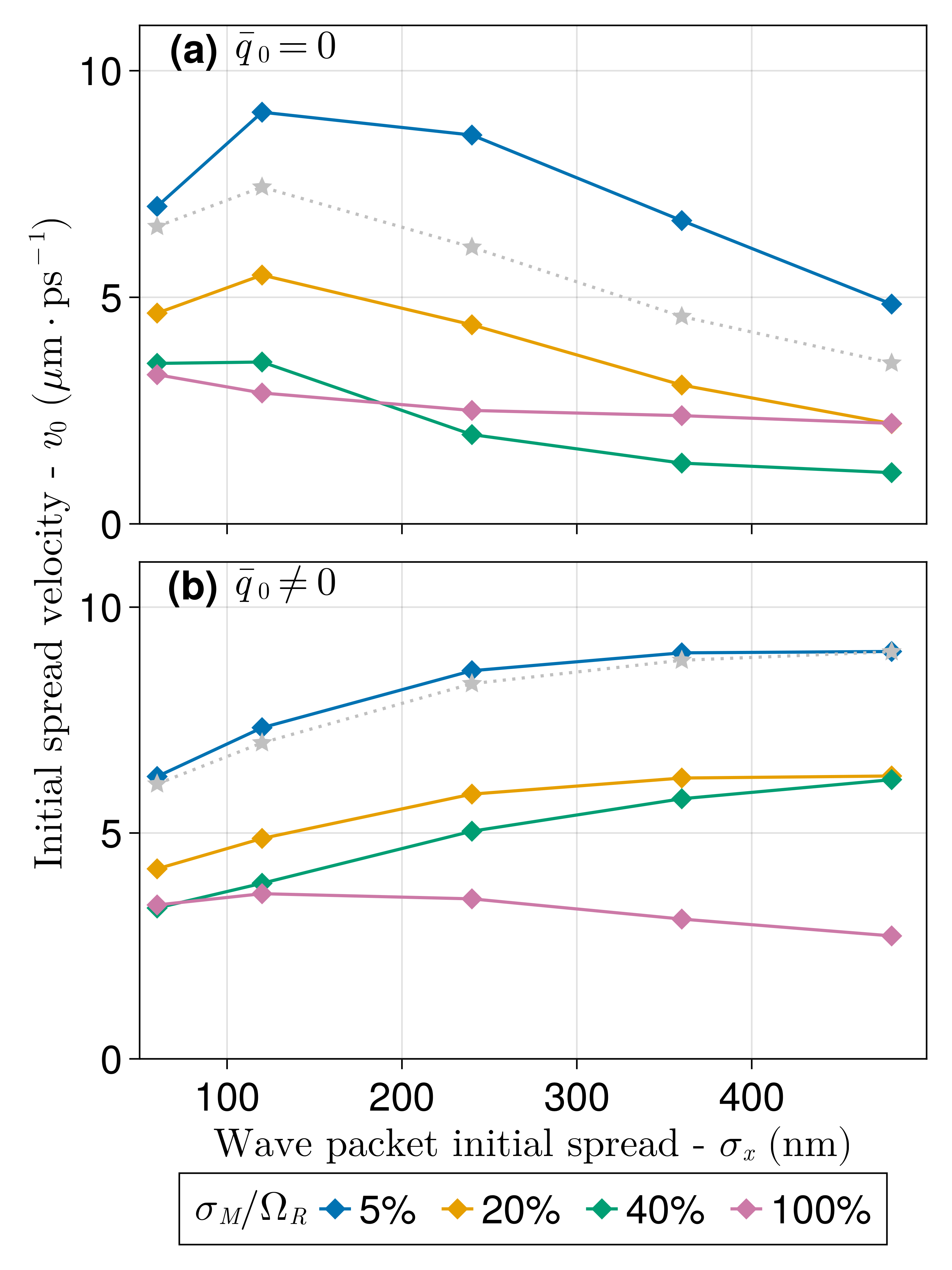
Figure 6: Initial spread velocity ($v_{0}$) dependency on the wave packet initial spread ($\sigma_{x}$) using different average momentum values: (a) $\bar{q}_{0}=0$ corresponding to the photon $\hbar\omega_{\bar{q}_{0}}=2.0$ eV and (b) $\bar{q}_{0}=0.0056$ nm^-1 corresponding to the photon $\hbar\omega_{\bar{q}_{0}}=2.1$ eV. Gray dotted curves are computed from Eq. 13.

To conclude, we investigate the effect of light-matter detuning $\delta=E_{M}-\hbar\omega_{0}$ on polariton-assisted exciton propagation. This study is motivated by detuning being a simple controllable microcavity parameter ¹, and by previous work which reported greater steady-state exciton migration probability under negative detuning (red-shifted cavities, where $E_{M}<\hbar\omega_{0})$⁴¹. We investigate the early dynamics in detuned microcavities by computing $v_{0}$ for a variable $E_{M}$ and fixed cavity lowest-energy mode $\hbar\omega_{0}=2.0~{}\text{eV}$. To gain insight into the long-time properties of the wave packet, we also show the maximum RMSD value observed over 5 ps.

In Fig. 7, we find detuning effects on $v_{0}$ and the maximum RMSD are very similar. Under weak disorder ($\sigma_{M}/\Omega_{R}<0.4$), both $v_{0}(\delta)$ and RMSD$(\delta)$ are peaked at $\delta=0$, i.e., the coherent exciton motion is faster when the cavity is in resonance with the dipolar excitation. This can be rationalized with Fig. 8a which shows a strong dependence of $v_{\alpha q}^{\text{eff}}$ on detuning. Blue-shifted microcavities lead to the slowest exciton motion as evidenced by the consistently smaller $v_{\alpha q}^{\text{eff}}$ obtained for $\delta=0.2$ eV in Fig. 8. On the other hand, red-shifted microcavities have small $v_{\alpha q}^{\text{eff}}$ at $q$ close to zero but higher values (compared to the resonant cavity) at sufficiently large $q$. Since the initial wave packets of Fig. 7 have $\bar{q}_{0}=0$, the dominant polariton contributions to the evolution are those for which $v_{\alpha q}^{\text{eff}}$ is larger at zero-detuning in comparison to the red-shifted case. Nevertheless, comparison between $v_{\alpha q}^{\text{eff}}$ at zero and negative detuning in Fig. 8b suggests that polariton-mediated exciton wave packet transport can be much faster in red-shifted cavities when the initial-state is prepared with $\bar{q}_{0}$ close to the maximum of $v_{\alpha q}^{\text{eff}}$.

In the presence of stronger disorder ($\sigma_{M}>0.4\Omega_{R})$, Fig. 7 shows the condition $\delta=0$ no longer provides a maximum RMSD and $v_{0}$, and the optimal detuning value is shifted toward negative values. Therefore, under sufficient disorder, red-shifting the microcavity enhances the exciton ballistic transport and the transport distance regardless of the initial wave packet preparation. This feature may be understood by noting in the presence of a significant amount of static disorder, many dipoles will have excitation energies below the lowest-energy microcavity mode. In this case, it becomes advantageous to employ negative detuning, since it supports lower energy photon modes that can interact resonantly with the dipoles with lower excitation energy. Conversely, raising $\hbar\omega_{0}-E_{M}$ to positive values leads to a reduction in the light-matter spectral overlap and, therefore, the maximum RMSD and $v_{0}$ consistently decrease as the microcavity is blue-shifted ($\delta>0$).

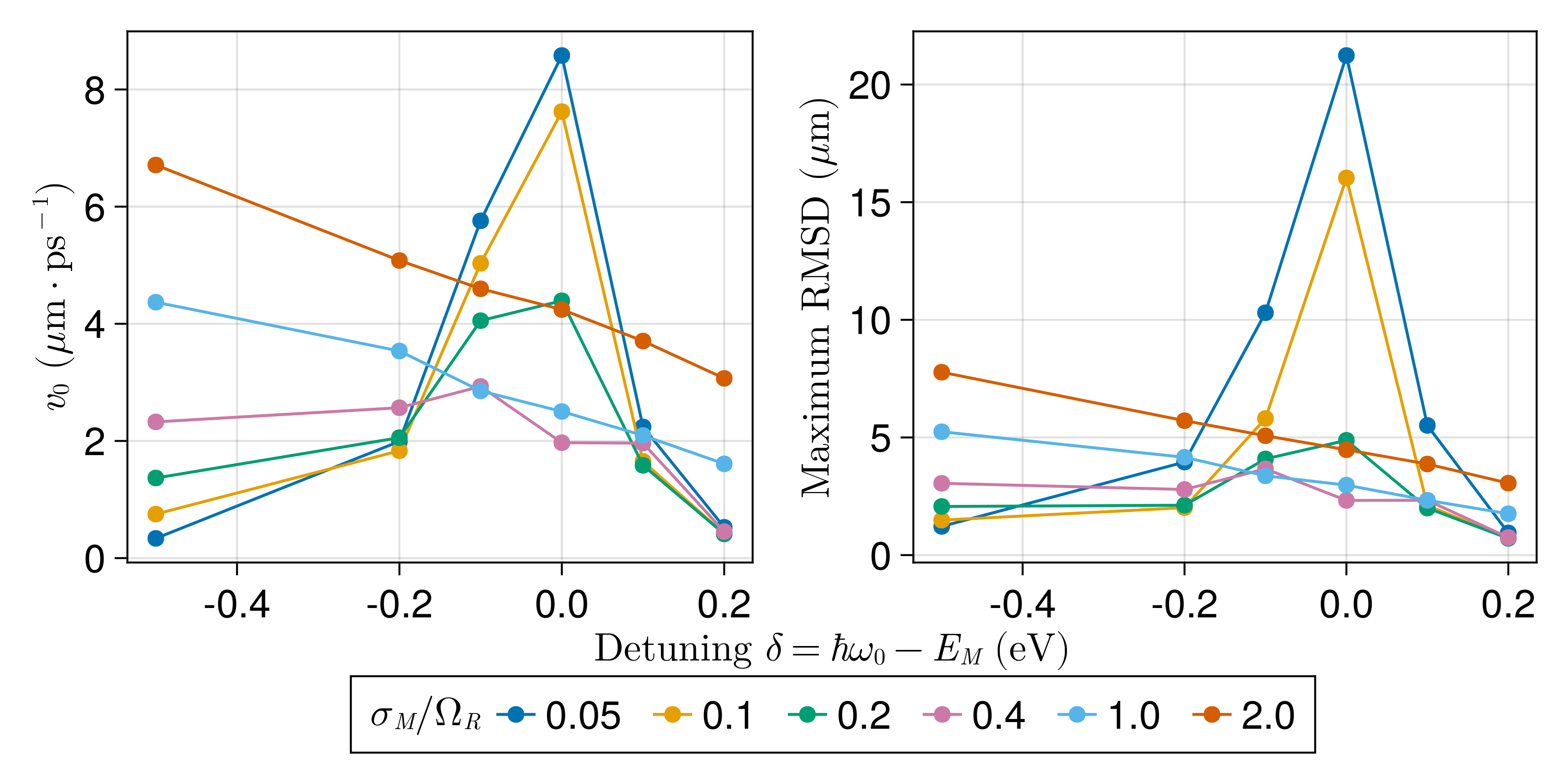
Figure 7: Disorder-dependent detuning effects on coherent exciton transport measured by (a) the initial spread velocity ($v_{0}$), and (b) the maximum RMSD over 5 ps. In all cases $\sigma_{x}=240$ nm and $\Omega_{R}=0.1$ eV. Each data point corresponds to an average over 100 disorder realizations.

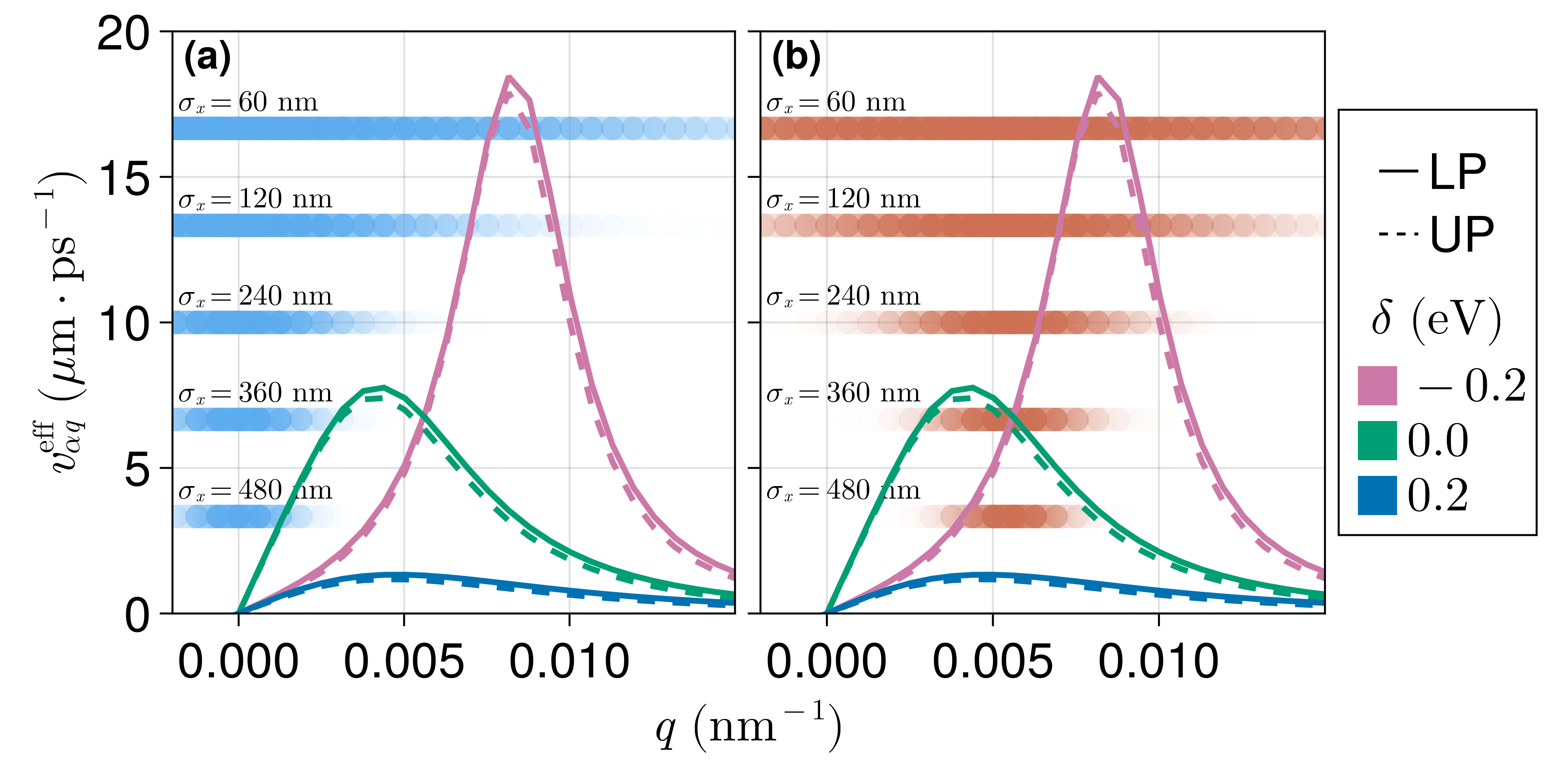
Figure 8: Effective group velocity (Eq. 14) for variable detuning $\delta=\hbar\omega_{0}-E_{M}$. Horizontal gradient bars represent the $P(q)$ distribution for distinct exciton wave packets (see Eq. 6) with (a) $\bar{q}_{0}=0.0$ and (b) $\bar{q}_{0}=0.0055$ nm^-1. The overlap between the gradient bars ($P(q)$) and the $v_{g}^{eff}$ curves yields the exciton spread velocity $v_{0}$ (Eq. 13). See text for more details.

Conclusions

We examined coherent polariton-mediated exciton transport on a lossless disordered polaritonic wire. Our analysis shows that the initial exciton wave packet (i.e., its spread and average momentum) strongly influences its ballistic propagation regime and may be optimized to maximize its early mobility. A striking contrast between polariton-mediated and purely excitonic transport was also noted here. Previous work showed that short-time direct exciton energy transport (via dipole-dipole interactions) is enhanced by disorder ³⁵. Here, we find, contrarily, that disorder systematically suppresses the initial wave packet spread. This implies a fundamental distinction in how disorder impacts coherent exciton energy transport inside and outside an optical microcavity.

We also analyzed the interplay of detuning and static disorder as factors impacting the ballistic transport regime. We found that while blue-shifted cavities always presented a slower exciton wave packet transport, red-shifted microcavities showed richer behavior, i.e., both suppression and enhancement of transport can be attained depending on the level of disorder and the initial state preparation.

To rationalize these results, we introduced the effective exciton group velocity $v_{\alpha q}^{\text{eff}}$, which can be computed from the system dispersion and the excitonic content of each polariton eigenmode. The early ballistic transport can be estimated by combining $v_{\alpha q}^{\text{eff}}$ with the initial exciton probability distribution in $q$ space. This analysis leads to a design principle for optimizing the initial exciton state for enhanced ultrafast coherent transport based on the complex interplay between disorder and tunable light-matter parameters such as detuning, Rabi splitting, and initial wave packet width and momentum. The optimal initial state for exciton transport must have: i) an initial wave vector matching the maximum value of the effective exciton group velocity and ii) a sufficiently narrow spread in $q$-space such that it only spans eigenmodes with large effective exciton group velocity.

Our theoretical analysis of exciton wave packet propagation in terms of the newly introduced effective exciton group velocity led to qualitative agreement with simulations even under moderate disorder ($\sigma_{M}/\Omega_{R}=0.4$). Such robustness and generalizability suggest our results will be useful for future theoretical and experimental studies of transport in optical cavities.

R.F.R. acknowledges generous start-up funds from the Emory University Department of Chemistry.

Symbol	Description	Value
$N_{M}$	Number of dipoles in the wire.	5000
$N_{c}$	Number of cavity modes used to describe the radiation field inside the cavity.	1001
$\Omega_{\text{R}}$	Rabi splitting: a measure of the collective light-matter interaction strength.	Variable
$a$	Intersite distance.	10 nm
$\sigma_{\text{a}}$	Standard deviation of sites positions.	1 nm
$E_{\text{M}}$	Dipole excitation energy.	Variable
$\sigma_{\text{M}}$	Standard deviation of the distribution of dipole excitation energies.	Variable
$L_{z}$	Wire length along $z$ dimension.	0.4 $\mu$m
$L_{y}$	Wire length along $y$ dimension.	0.2 $\mu$m
$L_{x}$	Wire length along $x$ dimension.	50 $\mu$m
$\epsilon$	Relative static permittivity.	3
$n_{y}$	Cavity quantum number associated with the $y$ dimension.	1
$n_{z}$	Cavity quantum number associated with the $z$ dimension.	1
$m_{x}$	Cavity quantum number associated with the $x$ dimension.	$\in\mathbb{Z}$
$q$	$x$-component of the wavevector $\mathbf{k}$	$2\pi m_{x}/L_{x}$.
$\sigma_{x}$	Initial wave packet width.	Variable
$\bar{q}_{0}$	Average initial exciton momentum along $x$	Variable

Table S1: List of symbols and notation used in this work

1 RMSD for a traveling exciton-polariton

1.1 Preliminary expressions

1.1.1 Wave packet representations

Before we proceed to our main problem, let us establish some intermediate results that will be useful later. First, consider the wave packet at $t=0$ represented in the position basis of $N_{M}$ dipoles

$$\ket{\psi_{0}}=\sum_{n=1}^{N_{M}}c_{n}\ket{n}\;.$$ (15)

Therefore, the probability of finding the $n$-th dipole excited is $|c_{n}|^{2}$. Note that in the main text, we use the notation $\ket{n;0}$ to represent the state where the $n$-th dipole is excited and no photon modes are populated. For simplicity, we use $\ket{n;0}\rightarrow\ket{n}$ here as the photonic degrees of freedom will not appear explicitly in the following expressions. We can transform $\ket{\psi_{0}}$ into its $k$-space representation using the resolution of the identity (in the exciton Hilbert space) $\sum_{k}\outerproduct{k}{k}=\text{$\mathds{1}$}_{E}$. That is,

$$\ket{\psi_{0}} =\sum_{k}\sum_{n=1}^{N_{M}}c_{n}\innerproduct{k}{n}\ket{k}\;,$$ (16)

$$=\sum_{k}\left(\frac{1}{\sqrt{N_{M}}}\sum_{n=1}^{N_{M}}c_{n}e^{-ikx_{n}}\right)\ket{k}\;,$$ (17)

where we have used $\innerproduct{k}{n}=\frac{e^{-ikx_{n}}}{\sqrt{N_{M}}}$. Defining

$$c_{k}=\frac{1}{\sqrt{N_{M}}}\sum_{n=1}^{N_{M}}c_{n}e^{-ikx_{n}}$$ (18)

we have the wave function in $k$-representation

$$\ket{\psi_{0}}=\sum_{k}c_{k}\ket{k}\;.$$ (19)

From the expression above, we see that the initial exciton probability distribution in wave number space is $P_{k}=|c_{k}|^{2}$.

1.1.2 Polariton Eigenstates

In the case where the dipole ensemble is translationally invariant, we can assign each eigenmode to the upper polariton (UP) branch if its energy is above the dipolar transition energy or lower polariton (LP) otherwise. The general Hamiltonian for the system can be block diagonalized using the transformation in Eq. 18. The resulting Hamiltonian is a direct sum of $2\times 2$ Hamiltonians where the $k$ wave number is preserved, that is, there is no mixing of different values of $k$. Using $q$ for the wave number of the polariton states we can write

$$\hat{H}\ket{\alpha q}=\hbar\omega_{\alpha q}\ket{\alpha q}\;,$$ (20)

where $\alpha$ is LP or UP. Moreover, the amplitude of the $n$-th dipole on the eigenstate $\ket{\alpha q}$ is

$$\innerproduct{n}{{\alpha q}}=-i\sqrt{\frac{\Pi_{\alpha q}}{N_{M}}}e^{iqx_{n}}\;,$$ (21)

where $\Pi_{\alpha q}=\sum_{n=1}^{N_{M}}\innerproduct{{\alpha q}}{n}\innerproduct{n}{{\alpha q}}$ is the total exciton content of the eigenstate $\ket{{\alpha q}}$. With this result, the overlap of each eigenstate with the initial wave packet is given by

$$\innerproduct{\psi_{0}}{{\alpha q}} =\sum_{n=1}^{N_{M}}c^{*}_{n}\innerproduct{n}{{\alpha q}}$$ (22)

$$=-i\sqrt{\Pi_{\alpha q}}\left(\frac{1}{\sqrt{N_{M}}}\sum_{n=1}^{N_{M}}c^{*}_{n}e^{iqx_{n}}\right)\;.$$ (23)

The term in brackets above is the complex conjugate of Eq. (18). Thus,

$$\innerproduct{\psi_{0}}{{\alpha q}}=-i\sqrt{\Pi_{\alpha q}}c^{*}_{q}\;.$$ (24)

The resolution of the identity in the eigenmode basis is given by

$$\text{$\mathds{1}$}=\sum_{\alpha}\sum_{q}\ket{{\alpha q}}\bra{{\alpha q}}\;.$$ (25)

1.1.3 Continuum limit

In what follows, we will take the thermodynamic limit where $L$ and $N_{M}$ go to infinity at the same rate, so $L/N_{M}$ is fixed. This will lead to closed-form expressions for excitonic observables in the absence of disorder. We will assume throughout that all relevant functions (of the dipole position $x_{n}=na$ and wavenumber $q$) are sufficiently slowly varying at the scale of the spatial lattice constant $x_{n+1}-x_{n}=\Delta x=a$ and reciprocal lattice spacing $\Delta q=2\pi/L$ so the continuum limit is well defined. We also assume the wave packet vanishes sufficiently fast outside a finite closed subset of position or wave number space. Under these conditions, any sum over discrete functions of the dipole position $x_{n}$ can be replaced by an integral over all space following

$$\sum_{n=1}^{N_{M}}f_{n}\rightarrow\frac{1}{a}\int f(x)\mathrm{d}x,$$ (26)

where $f(x)$ is the continuum representation of $f_{n}$ satisfying $f(x_{n})=f_{n}$. Likewise, the continuum limit for sums of discrete functions of $q$ is obtained from

$$\sum_{q}g_{q}\rightarrow\frac{L}{2\pi}\int~{}g(q)\mathrm{d}q,$$ (27)

where $g(q)$ is the continuum representation of $g_{q}$.

The continuum limit of the resolution of the identity in the eigenmode basis is given by

$$\text{$\mathds{1}$}=\frac{L}{2\pi}\sum_{\alpha}\int\ket{{\alpha q}}\bra{{\alpha q}}dq\;$$ (28)

Thus, it is convenient to redefine $\ket{{\alpha q}}$ following

$$\ket{{\alpha q}}\rightarrow\sqrt{\frac{2\pi}{L}}\ket{aq},$$ (29)

so as to recover the identity operator in the standard form

$$\text{$\mathds{1}$}=\sum_{\alpha}\int\ket{{\alpha q}}\bra{{\alpha q}}dq\;$$ (30)

Similar manipulations can be performed for the states living in the matter Hilbert space, e.g.,

$$\text{$\mathds{1}$}_{E}=\sum_{n=1}^{N_{M}}\ket{n}\bra{n}\rightarrow\frac{1}{a}\int\ket{x}\bra{x}\mathrm{d}x,$$ (31)

$$\text{$\mathds{1}$}_{E}=\sum_{q}\ket{q}\bra{q}\rightarrow\frac{L}{2\pi}\int\ket{q}\bra{q}\mathrm{d}q.$$ (32)

These identities suggest redefining the matter states in the continuum limit following

$$\ket{n}\rightarrow\sqrt{a}\ket{x},$$ (33)

$$\ket{q}\rightarrow\sqrt{\frac{2\pi}{L}}\ket{q}.$$ (34)

Using these relations, it follows in the continuum limit

$$\innerproduct{k}{x}=\sqrt{\frac{L}{2\pi a}}\innerproduct{k}{n}=\frac{e^{-ikx}}{\sqrt{2\pi}},$$ (35)

From these results, we obtain the wave packet representation in position and wave number space analogous to those of Sec. 1.1.1.

$$\ket{\psi_{0}}=\int c(x)\ket{x}\mathrm{d}x,~{}~{}c(x)=\innerproduct{x}{\psi_{0}}$$ (36)

$$\ket{\psi_{0}}=\int\int c(x)\innerproduct{q}{q}{x}~{}\ket{k}\mathrm{d}k\mathrm{d}x=\int c(k)\ket{k}\mathrm{d}k,$$ (37)

where the wave vector amplitude in the continuous wave number space is given by

$$c(k)=\frac{1}{\sqrt{2\pi}}\int c(x)e^{-ikx}\mathrm{d}x.$$ (38)

By performing the analogous transformations to the polariton eigenmodes we obtain

$$\innerproduct{x}{{\alpha q}}=-i\sqrt{\frac{\Pi_{{\alpha q}}}{2\pi}}e^{iqx},$$ (39)

$$\innerproduct{\psi_{0}}{{\alpha q}}=-i\sqrt{\Pi_{{\alpha q}}}c^{*}(q).$$ (40)

1.1.4 Time-evolved wave packet

The wave packet at an arbitrary time $\ket{\psi_{t}}$ can be written in terms of the initial state using the time-evolution operator

$$\ket{\psi_{t}}=e^{-i\hat{H}t/\hbar}\ket{\psi_{0}}\;.$$ (41)

Using the eigenstates discussed in the previous section, in particular Eq. 30, we can resolve the time evolution as

$$\ket{\psi_{t}}=\sum_{\alpha}\int_{-\infty}^{+\infty}e^{-i\hat{H}t/\hbar}\ket{{\alpha q}}\innerproduct{{\alpha q}}{\psi_{0}}dq\;.$$ (42)

Using Eq. 20 and 24 we get

$$\ket{\psi_{t}}=i\sum_{\alpha}\int_{-\infty}^{+\infty}\sqrt{\Pi_{\alpha q}}c(q)e^{-i\omega_{\alpha q}t}\ket{{\alpha q}}dq\;.$$ (43)

1.2 Exciton mean squared displacement

The exciton mean squared displacement $\Delta x_{E}^{2}$ can be written as

$$\Delta x_{E}^{2}(t) =\frac{1}{P_{M}(t)}\int|\innerproduct{x}{\psi_{t}}|^{2}(x-x_{0})^{2}\mathrm{d}x$$ (44)

$$P_{M}(t) =\int|\innerproduct{x}{\psi_{t}}|^{2}\mathrm{d}x\;,$$ (45)

where $x_{0}$ is the center of the initial wave packet. We start by computing $P_{M}(t)$ from the inner product of $\ket{x}$ with $\ket{\psi_{t}}$ (Eq. 43). The result is

$$\innerproduct{x}{\psi_{t}}=\frac{1}{\sqrt{2\pi}}\sum_{\alpha}\int_{-\infty}^{+\infty}\Pi_{\alpha q}c(q)e^{-i\omega_{\alpha q}t}e^{iqx}dq\;.$$ (46)

Hence,

$$P_{M} =\int\innerproduct{\psi_{t}}{x}\innerproduct{x}{\psi_{t}}\mathrm{d}x$$ (47)

$$=\frac{1}{2\pi}\sum_{\alpha}\sum_{\beta}\int_{-\infty}^{+\infty}\int_{-\infty}^{+\infty}c^{*}(q^{\prime})c(q)\Pi_{\beta q^{\prime}}\Pi_{\alpha q}e^{-i(\omega_{\alpha q}-\omega_{\beta q^{\prime}})t}\left(\int e^{i(q-q^{\prime})x}dx\right)dqdq^{\prime}\;.$$ (48)

Using $2\pi\delta(q-q^{\prime})=\int~{}\text{exp}[i(q-q^{\prime})x]dx$, we obtain

$$P_{M} =\sum_{\alpha}\sum_{\beta}\int_{-\infty}^{+\infty}|c(q)|^{2}\Pi_{\beta q}\Pi_{\alpha q}e^{-i(\omega_{\alpha q}-\omega_{{\beta q}})t}dq\;.$$ (49)

The double sum over $\alpha$ and $\beta$ produces four terms. Those are

$$P_{M} =\int_{-\infty}^{+\infty}|c(q)|^{2}\left(\Pi^{2}_{\text{LP}q}+\Pi^{2}_{\text{UP}q}+\Pi_{\text{LP}q}\Pi_{\text{UP}q}e^{-i(\omega_{\text{LP}q}-\omega_{\text{UP}q})t}+\Pi_{\text{LP}q}\Pi_{\text{UP}q}e^{-i(\omega_{\text{UP}q}-\omega_{\text{LP}q})t}\right)dq$$ (50)

$$=\int_{-\infty}^{+\infty}|c(q)|^{2}\left(\Pi^{2}_{\text{LP}q}+\Pi^{2}_{\text{UP}q}+2\Pi_{\text{LP}q}\Pi_{\text{UP}q}\cos{[(\omega_{\text{UP}q}-\omega_{\text{LP}q})t]}\right)dq\;.$$ (51)

As described in the main text, we measure the exciton spread velocity ($v_{0}$) by using a linear fit over the initial 500 fs. This process averages out the oscillating terms observed above. From now on, we ignore the time-dependent fluctuations of $P_{M}(t)$ and work with the more relevant time-averaged exciton content

$$\bar{P}_{M}=\int_{-\infty}^{+\infty}|c(q)|^{2}\left(\Pi^{2}_{\text{LP}q}+\Pi^{2}_{\text{UP}q}\right)dq\;.$$ (52)

Next, we analyze the remaining part of $\Delta x_{E}^{2}$. For the sake of simplicity and without loss of generality we assume $x_{0}=0$. We can use the results from Eq. 46 to write

$$P_{M}\Delta x_{E}^{2}(t) =\int|\innerproduct{x}{\psi_{t}}|^{2}x^{2}dx$$ (53)

$$=\frac{1}{2\pi}\sum_{\alpha}\sum_{\beta}\int_{-\infty}^{+\infty}\int_{-\infty}^{+\infty}c^{*}(q^{\prime})c(q)\Pi_{\beta q^{\prime}}\Pi_{\alpha q}e^{-i(\omega_{\alpha q}-\omega_{\beta q^{\prime}})t}\left(\int x^{2}e^{i(q-q^{\prime})x}dx\right)dqdq^{\prime}\;.$$ (54)

Rearranging the integrals and using the substitution $x^{2}e^{i(q-q^{\prime})x}=-\frac{\partial^{2}~{}}{\partial q^{2}}{e^{i(q-q^{\prime})x}}$, we obtain

$$P_{M}\Delta x_{E}^{2}(t) =-\frac{1}{2\pi}\sum_{\alpha}\sum_{\beta}\int_{-\infty}^{+\infty}c(q)\Pi_{\alpha q}e^{-i\omega_{\alpha q}t}\left(\int_{-\infty}^{+\infty}c^{*}(q^{\prime})\Pi_{\beta q^{\prime}}e^{i\omega_{\beta q^{\prime}}t}\frac{\partial^{2}}{\partial q^{2}}\left(\int e^{i(q-q^{\prime})x}dx\right)dq^{\prime}\right)dq$$ (55)

$$=-\sum_{\alpha}\sum_{\beta}\int_{-\infty}^{+\infty}c(q)\Pi_{\alpha q}e^{-i\omega_{\alpha q}t}\left(\int_{-\infty}^{+\infty}c^{*}(q^{\prime})\Pi_{\beta q^{\prime}}e^{i\omega_{\beta q^{\prime}}t}\frac{\partial^{2}}{\partial q^{2}}\delta(q-q^{\prime})dq^{\prime}\right)dq\;$$ (56)

Using the smoothness and compact support assumptions specified in our discussion of the continuum limit, it follows that

$$\int_{-\infty}^{+\infty}f(q^{\prime})\frac{\partial^{2}}{\partial q^{2}}\delta(q-q^{\prime})dq^{\prime}=\int_{-\infty}^{+\infty}\frac{\partial^{2}f(q^{\prime})}{\partial q^{2}}\delta(q-q^{\prime})dq^{\prime}=\frac{\partial^{2}f(q)}{\partial q^{2}}\;.$$ (57)

Therefore, we can reduce Eq. 56 to the form

$$P_{M}\Delta x_{E}^{2}(t) =-\sum_{\alpha}\sum_{\beta}\int_{-\infty}^{+\infty}c(q)\Pi_{\alpha q}e^{-i\omega_{\alpha q}t}\frac{\partial^{2}}{\partial q^{2}}\left[c^{*}(q)\Pi_{\beta q}e^{i\omega_{{\beta q}}t}\right]dq\;.$$ (58)

To proceed, we evaluate the second derivative with respect to $q$

$$e^{-i\omega_{\beta q}t}\frac{\partial^{2}}{\partial q^{2}}\left[c^{*}(q)\Pi_{\beta q}e^{i\omega_{{\beta q}}t}\right] =e^{-i\omega_{\beta q}t}\frac{\partial}{\partial q}\left[\frac{\partial c^{*}(q)\Pi_{\beta q}}{\partial q}e^{i\omega_{{\beta q}}t}+{-i\frac{\partial\omega_{{{\beta q}}}}{\partial q}t}c^{*}(q)\Pi_{\beta q}e^{i\omega_{{\beta q}}t}\right]$$

$$=\frac{\partial^{2}~{}}{\partial q^{2}}{[c^{*}(q)\Pi_{\beta q}]}-2it\frac{\partial\omega_{{{\beta q}}}}{\partial q}\frac{\partial}{\partial q}[c^{*}(q)\Pi_{\beta q}]-tc^{*}(q)\Pi_{\beta q}\left[i\frac{\partial^{2}\omega_{{{\beta q}}}}{\partial q^{2}}+t\left(\frac{\partial\omega_{{{\beta q}}}}{\partial q}\right)^{2}\right].$$ (59)

To obtain a more compact expression, we define

$$\Delta_{\beta\alpha}(q) =\omega_{{\beta q}}-\omega_{\alpha q},$$ (60)

$$\gamma_{{\alpha q}} =c(q)\Pi_{\alpha q},$$ (61)

$$\gamma_{{{\beta q}}}^{*} =c^{*}(q)\Pi_{\beta q},$$ (62)

$$v_{g}^{{{\beta q}}} =\frac{\partial\omega_{{\beta q}}}{\partial q}.$$ (63)

Using these definitions and plugging Eq. 59 into Eq. 58 we get

$$P_{M}\Delta x_{E}^{2}(t) =-\sum_{\alpha}\sum_{\beta}\int_{-\infty}^{+\infty}\left(\frac{\partial^{2}\gamma^{*}_{{{\beta q}}}}{\partial q^{2}}-it\frac{\partial v_{g}^{{{\beta q}}}}{\partial q}\gamma_{{{\beta q}}}^{*}-2iv_{g}^{{{\beta q}}}t\frac{\partial~{}\gamma^{*}_{{{\beta q}}}}{\partial q}-(v_{g}^{{{\beta q}}}t)^{2}\gamma^{*}_{{{\beta q}}}\right)\gamma_{{\alpha q}}e^{i\Delta_{\beta\alpha}(q)t}dq$$ (64)

Since our goal is to obtain the term of $\sqrt{\Delta x_{E}^{2}}$ proportional to $t$, we will ignore the cross LP-UP oscillating terms where $\beta\neq\alpha$ (note this is consistent with our neglect of oscillations in the previous treatment of $P_{M}$). It follows in this case that

$$P_{M}\Delta x_{E}^{2}(t) =-\sum_{\alpha}\int_{-\infty}^{+\infty}\left[\left(\frac{\partial^{2}~{}}{\partial q^{2}}\gamma^{*}_{{\alpha q}}\right)\gamma_{{\alpha q}}-it\left(\frac{\partial~{}}{\partial q}v_{g}^{{\alpha q}}\right)|\gamma_{{\alpha q}}|^{2}-2itv_{g}^{{\alpha q}}\left(\frac{\partial~{}}{\partial q}\gamma^{*}_{{\alpha q}}\right)\gamma_{{\alpha q}}-(v_{g}^{{\alpha q}}t)^{2}|\gamma_{{\alpha q}}|^{2}\right]dq\;$$ (65)

Note from the above expression that the time-independent contribution gives the exciton spread at $t=0$ i.e.,

$$P_{M}\Delta x_{E}^{2}(0)=-\sum_{\alpha}\int_{-\infty}^{+\infty}\left(\frac{\partial^{2}~{}}{\partial q^{2}}\gamma^{*}_{{\alpha q}}\right)\gamma_{{\alpha q}}dq.$$ (66)

It can be shown with integration by parts that the $\mathcal{O}(t)$ term in Eq. 65 is given by

$$itv_{g}^{{\alpha q}}\left(\frac{\partial}{\partial q}\gamma_{{\alpha q}}\right)\gamma_{{\alpha q}}^{*}-itv_{g}^{{\alpha q}}\left(\frac{\partial}{\partial q}\gamma_{{\alpha q}}^{*}\right)\gamma_{{\alpha q}}=-2v_{g}^{{\alpha q}}t\times\text{Im}\left[\gamma_{{\alpha q}}^{*}\frac{\partial}{\partial q}\gamma_{{\alpha q}}\right]$$ (67)

Hence, it can be seen that if $\gamma_{{\alpha q}}=c_{q}\Pi_{\alpha q}$ is real this term vanishes. In the case of Gaussian wave packets in the continuum limit, we have

$$c(q)=\frac{1}{\sqrt{2\pi}}\int_{-\infty}^{+\infty}c(x)e^{-iqx}dx=\frac{1}{2\pi\sigma_{x}}\int_{-\infty}^{+\infty}e^{-\frac{(x-x_{0})^{2}}{2\sigma_{x}}}e^{i(\bar{q}_{0}-q)x}dx$$ (68)

$$\frac{1}{2\pi\sigma_{x}}\int_{-\infty}^{+\infty}e^{-\frac{(x-x_{0})^{2}}{2\sigma_{x}}}[\cos{(\bar{q}_{0}-q)x}+i\sin{(\bar{q}_{0}-q)x}]dx\;.$$ (69)

Due to parity considerations, the sine part of this expression vanishes and $c(q)$ must be real. Consequently, Eq. 67 is zero for Gaussian wave packets.

It follows that the ballistic spread velocity $v_{0}$ for a Gaussian wave packet is given by

$$v_{0}^{2}=\frac{\Delta x_{E}^{2}(t)-\Delta x_{E}^{2}(0)}{t^{2}}=\frac{1}{P_{M}}\int_{-\infty}^{+\infty}|c(q)|^{2}\left[\left(v_{g}^{\text{LP}}(q)\Pi_{\text{LP}q}\right)^{2}+\left(v_{g}^{\text{UP}}(q)\Pi_{\text{UP}q}\right)^{2}\right]dq\;.$$ (70)

Defining an effective group velocity as $v_{\alpha q}^{\text{eff}}=v_{g}^{\alpha}(q)\Pi_{\alpha q}$ and disregarding the (here constant) prefactor $P_{M}$ we arrive at the following final estimate for the observed ballistic exciton spread velocity

$$v_{0}^{2}\approx\int_{-\infty}^{+\infty}|c(q)|^{2}\left[(v_{\text{LP}q}^{\text{eff}})^{2}+(v_{\text{UP}q}^{\text{eff}})^{2}\right]dq\;.$$ (71)

2 Exciton escape probability

In this section, we obtain insight into the exciton escape probability defined in the main text as

$$\chi(t)=1-\frac{1}{P_{M}(t)}\sum_{n\in\mathcal{I}}|\innerproduct{n}{\psi(t)}|^{2},$$ (72)

where $\mathcal{I}$ is the integer interval $[n_{\text{min}},n_{\text{max}}]$ containing the indices of the dipoles comprising $99\%$ of the initial wave packet probability. For the sake of simplicity, we ignore $P_{M}(t)$ below since both at very early times $t\rightarrow 0$ and late times $t\rightarrow\infty$, $P_{M}(t)$ is approximately constant. Let $P_{n}(t)$ denote the time-dependent probability to to detect an exciton at the $n$th site and $\{\ket{A},\ket{B},...\}$ correspond to the set of eigenstates of $H$ with eigenvalues $E_{A}=\hbar\omega_{A}$, etc. It follows that we can write the probability $P_{n}(t)$ to detect an exciton at the $n$th site at time $t$ is given by

$$P_{n}(t) =|\innerproduct{n}{\psi(t)}|^{2}=\left|\sum_{A}\innerproduct{n}{A}\innerproduct{A}{\psi_{0}}e^{-i\omega_{A}t}\right|^{2}$$

$$=\left|\sum_{A}\sum_{m_{1}}A_{n}A_{m_{1}}^{*}c_{m_{1}}e^{-i\omega_{A}t}\right|^{2}$$

$$=\sum_{A,B}\sum_{m_{1},m_{2}}A_{n}A_{m_{1}}^{*}B_{n}^{*}B_{m_{2}}c_{m_{1}}c_{m_{2}}^{*}e^{-i(\omega_{A}-\omega_{B})t}.$$ (73)

where $A_{n}$ corresponds to the probability amplitude to detect an exciton at site $\ket{n}$ when the system is in eigenstate $\ket{A}$, and $c_{n}=\innerproduct{n}{\psi_{0}}$ as in the previous section. We can decompose $P_{n}(t)$ into

$$P_{n}(t)=P_{n}+\Delta P_{n}(t),$$ (74)

where $P_{n}$ corresponds to the time-independent asymptotic part and $\Delta P_{n}(t)$ is the time-fluctuating contribution to $P_{n}(t)$. Each of these terms is given explicitly by

$$P_{n}=\sum_{A}\sum_{m_{1},m_{2}}|A_{n}|^{2}A_{m_{1}}^{*}A_{m_{2}}c_{m_{1}}c_{m_{2}}^{*},$$ (75)

$$\Delta P_{n}(t)=\sum_{A}\sum_{B\neq A}\sum_{m_{1},m_{2}}A_{n}A_{m_{1}}^{*}B_{n}^{*}B_{m_{2}}c_{m_{1}}c_{m_{2}}^{*}e^{-i(\omega_{A}-\omega_{B})t}.$$ (76)

Given the definition of $\chi(t)$ in Eq. 72, it follows that we may also define an asymptotic time-independent part contribution $\chi$ and an oscillatory contribution $\Delta\chi(t)$ such that $\chi(t)=\chi+\Delta\chi(t)$ given by

$$\chi\approx 1-\sum_{A}\sum_{n\in\mathcal{I}}\sum_{m_{1},m_{2}}|A_{n}|^{2}A_{m_{1}}^{*}A_{m_{2}}c_{m_{1}}c_{m_{2}}^{*},$$ (77)

$$\Delta\chi(t)\approx-\sum_{A}\sum_{B\neq A}\sum_{n\in\mathcal{I}}\sum_{m_{1},m_{2}}A_{n}A_{m_{1}}^{*}B_{n}^{*}B_{m_{2}}c_{m_{1}}c_{m_{2}}^{*}e^{-i(\omega_{A}-\omega_{B})t},$$ (78)

where the approximate character of the identities emphasizes our neglect of $P_{M}(t)$ in the definition of $\chi(t)$. We examine $\chi$ and $\Delta\chi(t)$ next starting with the time-independent term which we rewrite as

$$\chi =1-\sum_{A}\sum_{n\in\mathcal{I}}|A_{n}|^{4}|c_{n}|^{2}-\sum_{A}\sum_{n\in\mathcal{I}}\sum_{m\neq n}|A_{n}|^{2}|A_{m}|^{2}|c_{m}|^{2}$$

$$-\sum_{A}\sum_{n\in\mathcal{I}}\sum_{m\neq n}|A_{n}|^{2}\left(A_{n}^{*}A_{m}c_{n}c_{m}^{*}+A_{m}^{*}A_{n}c_{m}c_{n}^{*}\right)-\sum_{A}\sum_{n\in\mathcal{I}}\sum_{m_{1}\neq n}\sum_{m_{2}\neq m_{1},n}|A_{n}|^{2}A_{m_{1}}^{*}A_{m_{2}}c_{m_{1}}c_{m_{2}}^{*}.$$ (79)

The fluctuating term can be written likewise as

$$\Delta\chi(t)= -\sum_{A}\sum_{B\neq A}\sum_{n\in\mathcal{I}}|A_{n}|^{2}|B_{n}|^{2}|c_{n}|^{2}\text{cos}[(\omega_{A}-\omega_{B})t]$$

$$-\sum_{A}\sum_{B\neq A}\sum_{n\in\mathcal{I}}\sum_{m\neq n}\left(A_{n}A_{m}^{*}B_{n}^{*}B_{m}|c_{m}|^{2}+|A_{n}|^{2}B_{n}^{*}B_{m}c_{n}c_{m}^{*}+A_{n}A_{m}^{*}|B_{n}|^{2}c_{m}c_{n}^{*}\right)e^{-i(\omega_{A}-\omega_{B})t}$$

$$-\sum_{A}\sum_{B\neq A}\sum_{n\in\mathcal{I}}\sum_{m_{1}\neq n}\sum_{m_{2}\neq m_{1},n}A_{n}A_{m_{1}}^{*}B_{n}^{*}B_{m_{2}}c_{m_{1}}c_{m_{2}}^{*}e^{-i(\omega_{A}-\omega_{B})t}.$$ (80)

Note that

$$\frac{\mathrm{d}}{\mathrm{d}t}\chi(t)=\frac{\mathrm{d}}{\mathrm{d}t}\Delta\chi(t),$$ (81)

and $\mathrm{d}\Delta\chi(t)/\mathrm{d}t\rightarrow 0$ as $t\rightarrow 0^{+}$. Therefore, the early growth of $\chi(t)$ is characterized by

$$G=\lim_{t\rightarrow 0^{+}}\frac{1}{2}\frac{\mathrm{d}^{2}}{\mathrm{d}t^{2}}\Delta\chi(t).$$ (82)

Strong disorder limit. To simplify, we perform the disorder average of $\chi$ which we denote by $\overline{\chi}$ (our notation for disorder average of a quantity $f$ in this section is given by $\overline{f}$). Under sufficiently strong disorder ($\sigma_{M}\gg\Omega_{R}$), we expect $\overline{A_{m_{1}}^{*}A_{m_{2}}}\approx|\overline{A_{m_{1}}}|^{2}\delta_{m_{1},m_{2}}$ for any eigenmode $A$, and therefore the disorder-averaged exciton escape probability components satisfy

$$\overline{\chi}\approx 1-\sum_{A}\sum_{n\in\mathcal{I}}\overline{|A_{n}|^{4}}|c_{n}|^{2}-\sum_{A}\sum_{n\in\mathcal{I}}\sum_{m\neq n}\overline{|A_{n}|^{2}}~{}\overline{|A_{m}|^{2}}|c_{m}|^{2},$$ (83)

$$\overline{\Delta\chi(t)}\approx-\sum_{A}\sum_{B\neq A}\sum_{n\in\mathcal{I}}\overline{|A_{n}|^{2}|B_{n}|^{2}}|c_{n}|^{2}\text{cos}\left[(\omega_{A}-\omega_{B})t\right].$$ (84)

From the last equation, we directly quantify the early growth of the escape probability from

$$\overline{G}\approx\frac{1}{2}\sum_{A}\sum_{B\neq A}\sum_{n\in\mathcal{I}}\overline{|A_{n}|^{2}|B_{n}|^{2}}|c_{n}|^{2}(\omega_{A}-\omega_{B})^{2}.$$ (85)

Weak disorder limit. In the weak disorder case,

$$G=\frac{1}{2}\sum_{A}\sum_{B\neq A}\sum_{n\in\mathcal{I}}\sum_{m_{1},m_{2}}A_{n}A_{m_{1}}^{*}B_{n}^{*}B_{m_{2}}c_{m_{1}}c_{m_{2}}^{*}(\omega_{A}-\omega_{B})^{2}$$ (86)

Assuming only modes with $q\sigma_{x}\ll 1$ contribute significantly, we can take the long wavelength limit and ignore the phase difference of eigenmode amplitudes in distinct sites, thus considerably simplifying $G$

$$G\approx\frac{1}{2N_{\mathcal{I}}}\sum_{A}\sum_{B\neq A}\sum_{n\in\mathcal{I}}\sum_{m_{1},m_{2}}|A_{n}|^{2}|B_{n}|^{2}(\omega_{A}-\omega_{B})^{2},$$ (87)

where we made the replacement $c_{m_{1}}c_{m_{2}}^{*}\approx 1/N_{\mathcal{I}}$ and $N_{\mathcal{I}}$ is the number of elements of $\mathcal{I}$.

3 Wave packets under DET

In Figs. S1, S2, and S3 we show snapshots of the exciton wave packet at different time steps where we can see the different in the wave packet shape under disorder enhanced transport (DET). In Figs. S1-S3(a) we see that under very strong disorder ($\sigma_{M}/\Omega_{R}>1$) the wave packet decays more quickly in space, but has a more delocalized tail. This decolalization is captured in the RMSD but not in the migration probability ($\chi$) as seen in S1-S3(b).

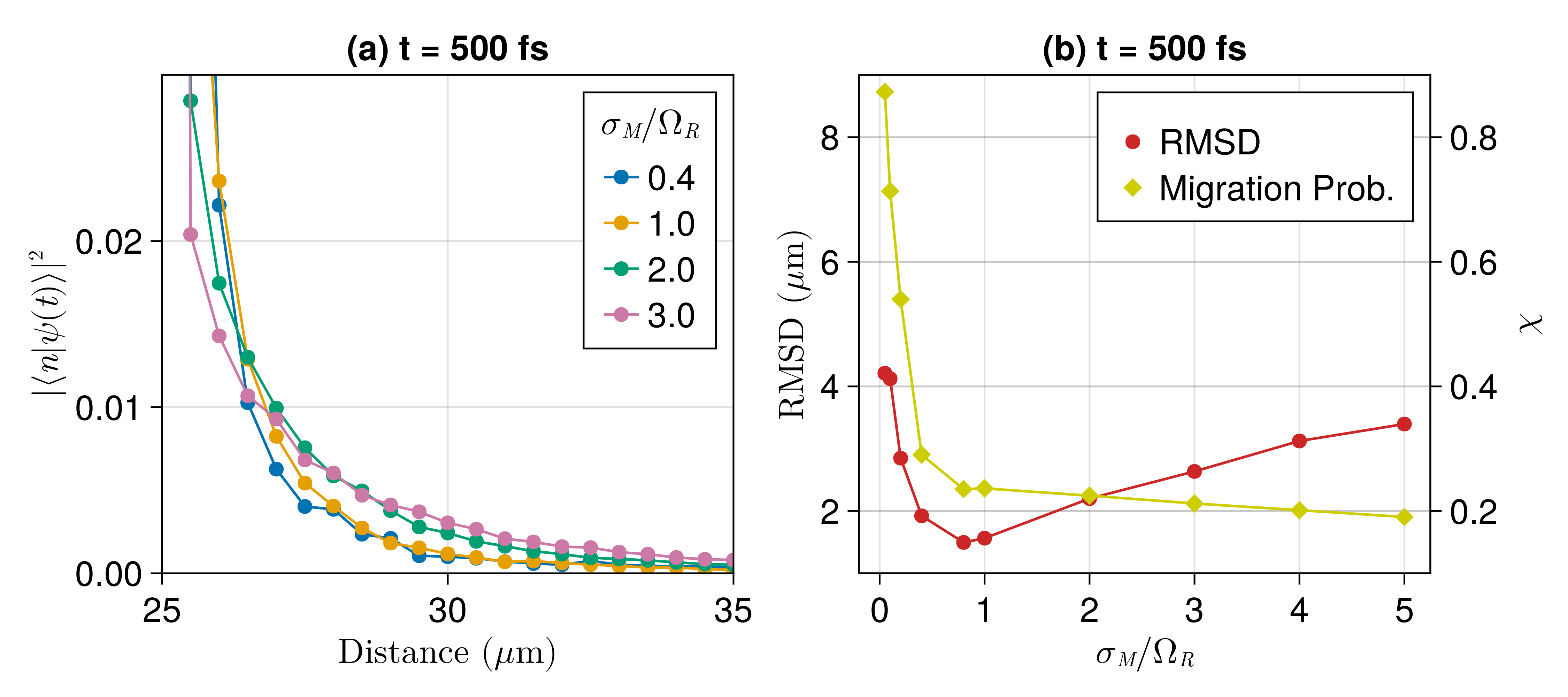
Figure S1: Wave packet properties at $t=500$ fs: (a) Decay as a function of distance at different relative disorder strengths. (b) RMSD and migration probabilities at a fixed time step at different disorder strengths. In all cases, $\Omega_{R}=0.1$ eV and $\sigma_{x}=120$ nm. Other parameters are fixed as in the main text.

‘

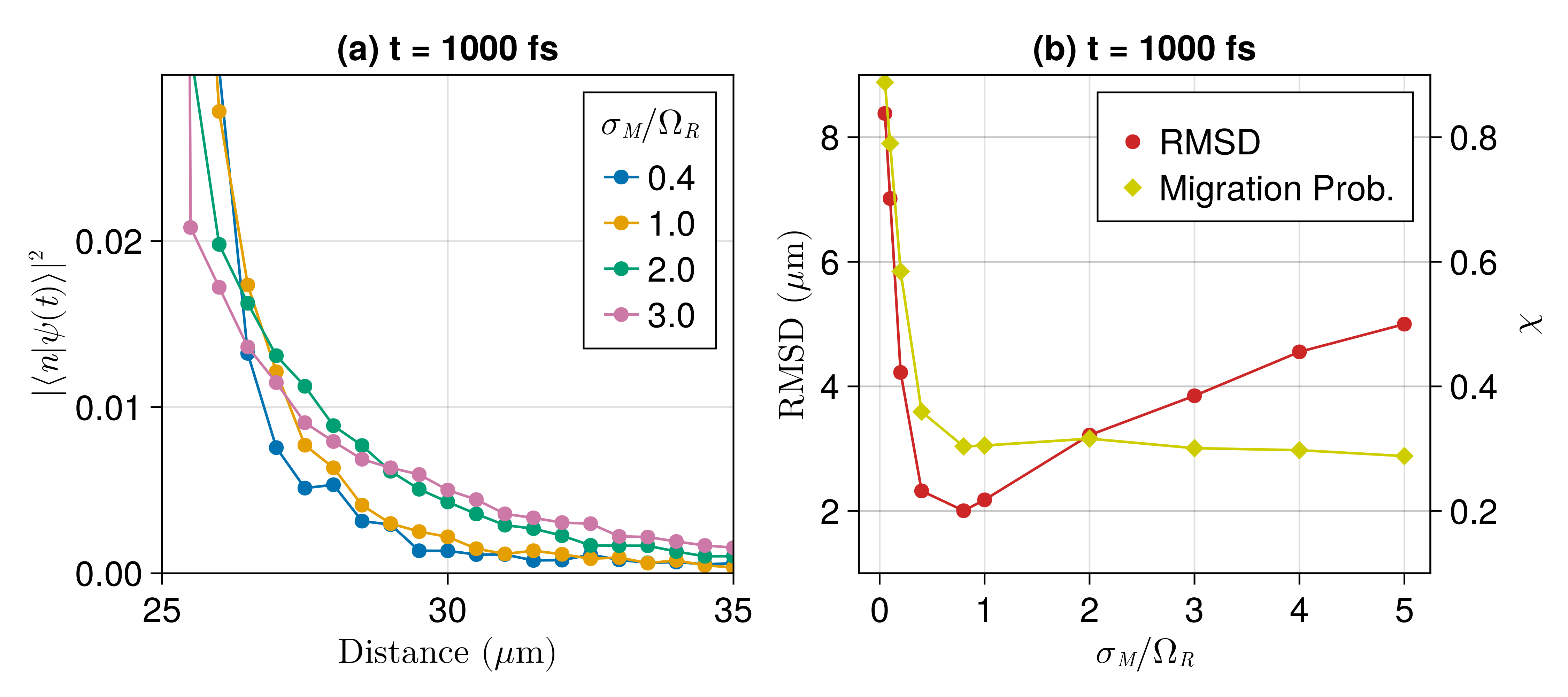
Figure S2: Wave packet properties at $t=1000$ fs: (a) Decay as a function of distance at different relative disorder strengths. (b) RMSD and migration probabilities at a fixed time step at different disorder strengths. In all cases, $\Omega_{R}=0.1$ eV and $\sigma_{x}=120$ nm. Other parameters are fixed as in the main text.

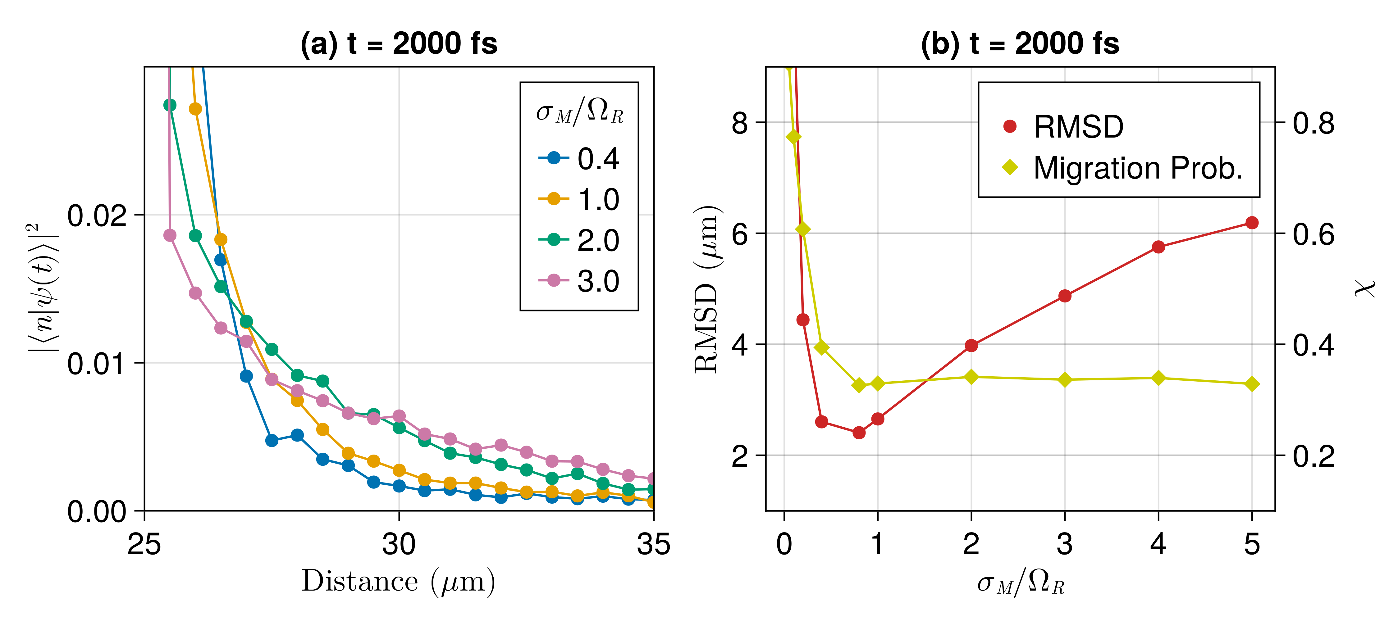
Figure S3: Wave packet properties at $t=2000$ fs: (a) Decay as a function of distance at different relative disorder strengths. (b) RMSD and migration probabilities at a fixed time step at different disorder strengths. In all cases, $\Omega_{R}=0.1$ eV and $\sigma_{x}=120$ nm. Other parameters are fixed as in the main text.

4 Propagation Profiles

Figs. S4-S7 shows the time evolution of the RMSD and migration probability ($\chi$) defined in the main text and repeated below for reference

$$\text{RMSD}(t) =\left[\frac{1}{P_{\text{M}}(t)}\sum_{n}^{N_{M}}|\bra{n;0}\ket{\psi(t)}|^{2}(x_{n}-x_{0})^{2}\right]^{1/2}\,,$$ (88)

$$P_{\text{M}}(t) =\sum_{n}^{N_{M}}|\bra{n;0}\ket{\psi(t)}|^{2}\,.$$ (89)

$$\chi(t) =1-\frac{1}{P_{\text{M}}(t)}\sum_{n=n_{\text{min}}}^{n_{\text{max}}}|\bra{n;0}\ket{\psi(t)}|^{2}\,.$$ (90)

It can be seen that the time to reach a steady state (constant RMSD) decreases as the Rabi splitting is increased.

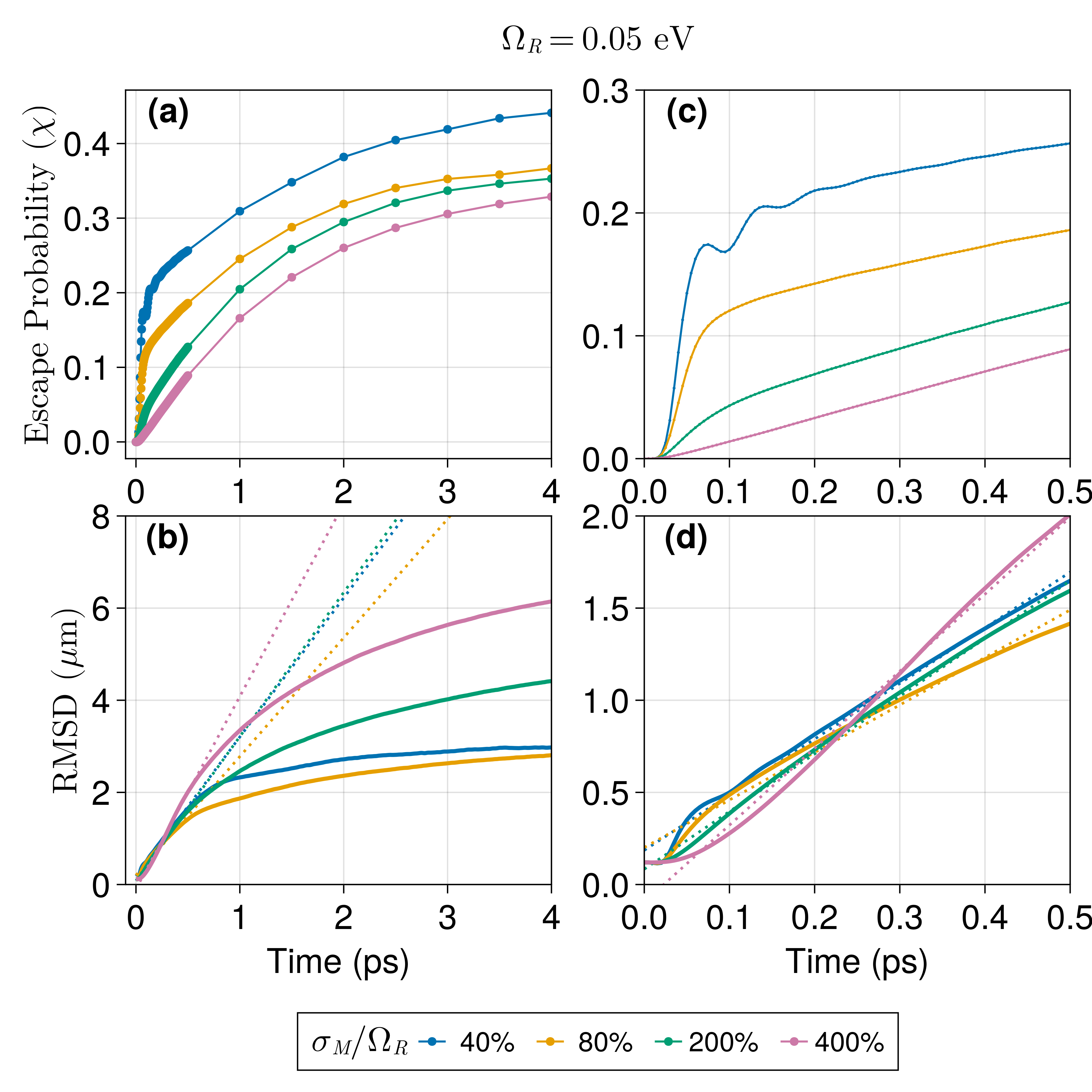
Figure S4: Propagation of exciton wave packets at different disorder strengths measured by (a) escape probability (Eq. 10) and (b) RMSD (Eq. 8). In all cases, $\sigma_{x}=120$ nm and $\Omega_{R}=0.05$ eV. Results are averages of 100 disordered realizations. The dotted lines in (b) are linear fits on the early propagation ($\leq$ 500 fs) from which slopes are used to measure the initial ballistic velocity ($v_{0}$). Panels (c) and (d) are zoomed in versions of (a) and (b), respectively.

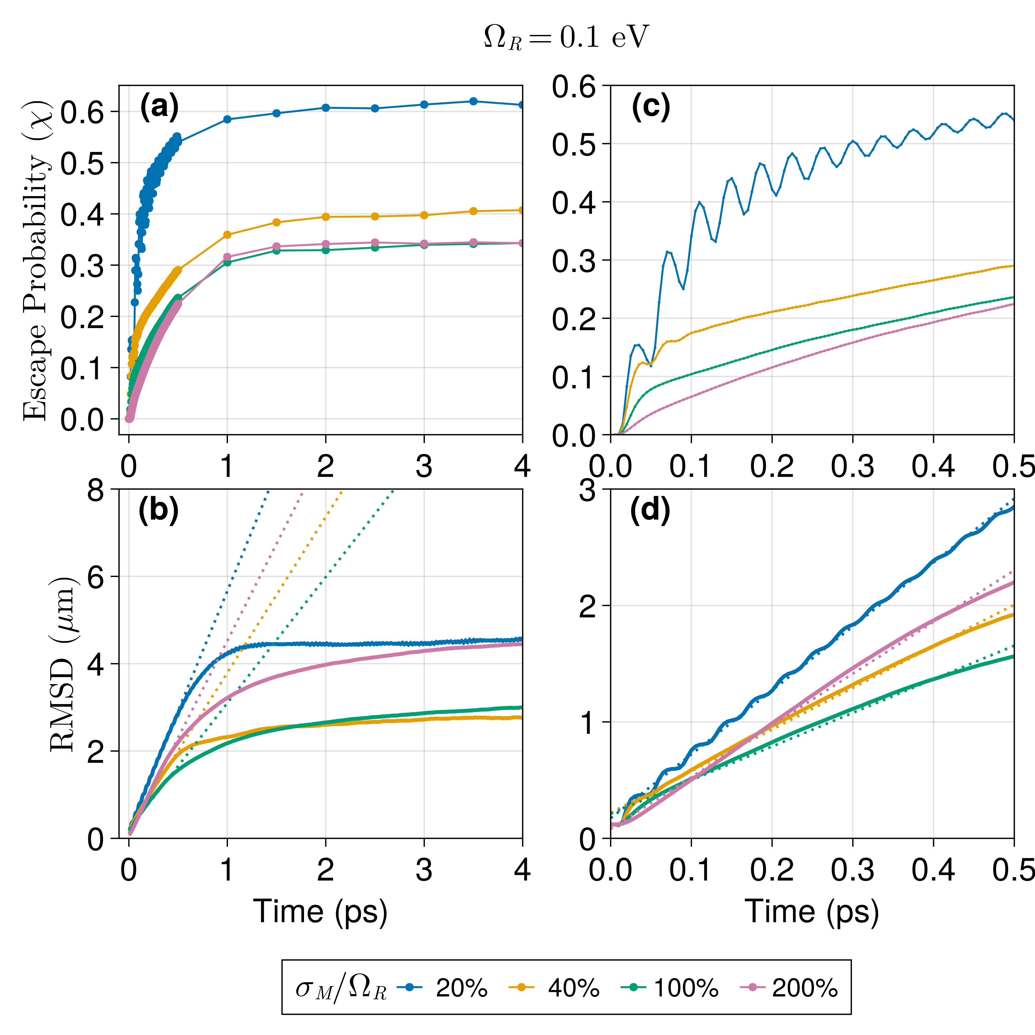
Figure S5: Propagation of exciton wave packets at different disorder strengths measured by (a) escape probability (Eq. 10) and (b) RMSD (Eq. 8). In all cases, $\sigma_{x}=120$ nm and $\Omega_{R}=0.1$ eV. Results are averages of 100 disordered realizations. The dotted lines in (b) are linear fits on the early propagation ($\leq$ 500 fs) from which slopes are used to measure the initial ballistic velocity ($v_{0}$). Panels (c) and (d) are zoomed in versions of (a) and (b), respectively.

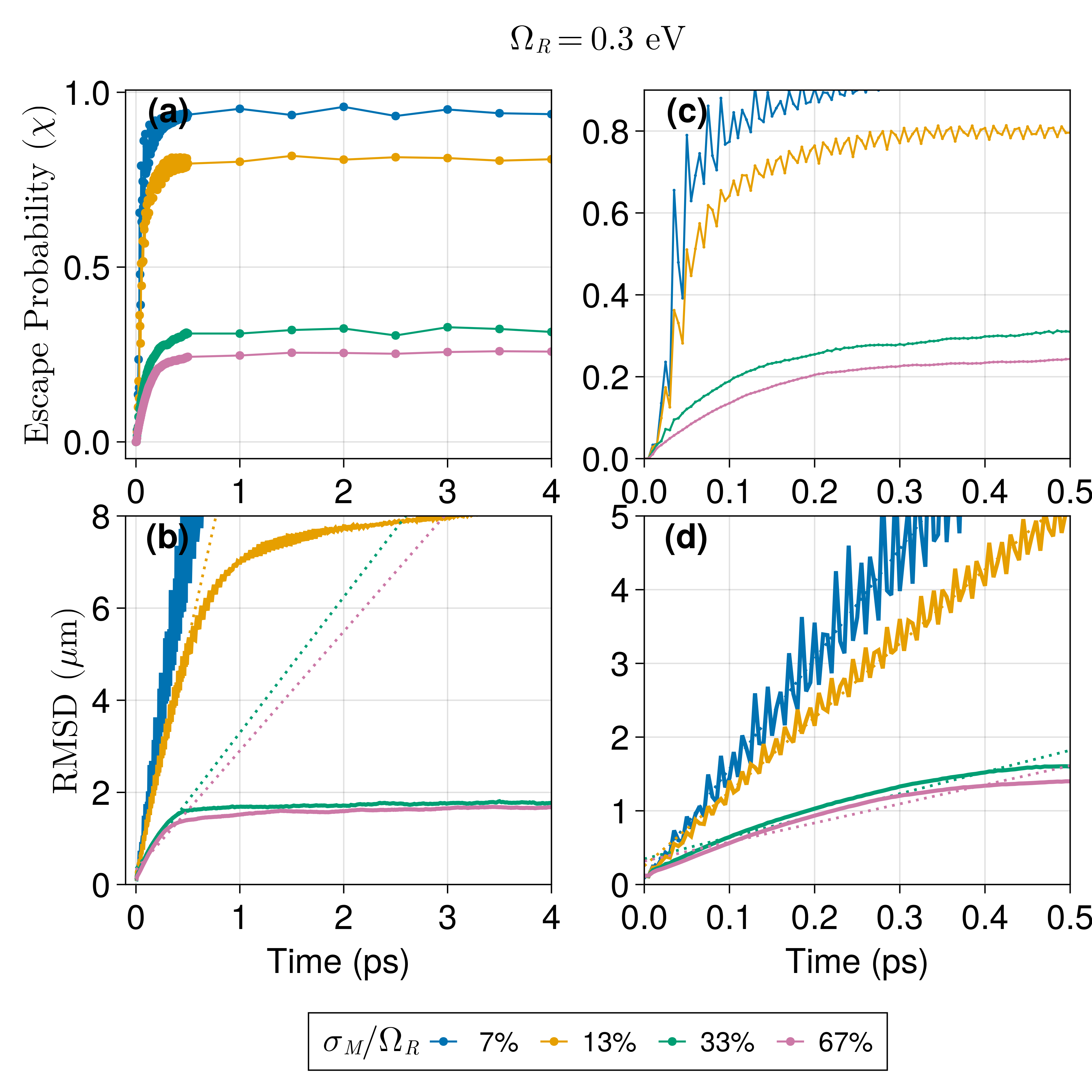
Figure S7: Propagation of exciton wave packets at different disorder strengths measured by (a) escape probability (Eq. 10) and (b) RMSD (Eq. 8). In all cases, $\sigma_{x}=120$ nm and $\Omega_{R}=0.3$ eV. Results are averages of 100 disordered realizations. The dotted lines in (b) are linear fits on the early propagation ($\leq$ 500 fs) from which slopes are used to measure the initial ballistic velocity ($v_{0}$). Panels (c) and (d) are zoomed in versions of (a) and (b), respectively.

References

- Kavokin et al. 2017 Kavokin, A. V.; Baumberg, J. J.; Malpuech, G.; Laussy, F. P. Microcavities; Oxford University Press: London, 2017
- Yu et al. 2018 Yu, X.; Yuan, Y.; Xu, J.; Yong, K.-T.; Qu, J.; Song, J. Strong Coupling in Microcavity Structures: Principle, Design, and Practical Application. Laser Photonics Rev. 2018, 13, 1800219
- Tibben et al. 2023 Tibben, D. J.; Bonin, G. O.; Cho, I.; Lakhwani, G.; Hutchison, J.; Gómez, D. E. Molecular Energy Transfer under the Strong Light–Matter Interaction Regime. Chem. Rev. 2023, 123, 8044–8068
- Coles et al. 2014 Coles, D. M.; Somaschi, N.; Michetti, P.; Clark, C.; Lagoudakis, P. G.; Savvidis, P. G.; Lidzey, D. G. Polariton-mediated energy transfer between organic dyes in a strongly coupled optical microcavity. Nat. Mater. 2014, 13, 712–719
- Zhong et al. 2016 Zhong, X.; Chervy, T.; Wang, S.; George, J.; Thomas, A.; Hutchison, J. A.; Devaux, E.; Genet, C.; Ebbesen, T. W. Non-Radiative Energy Transfer Mediated by Hybrid Light-Matter States. Angew. Chem., Int. Ed. 2016, 55, 6202–6206
- Zhong et al. 2017 Zhong, X.; Chervy, T.; Zhang, L.; Thomas, A.; George, J.; Genet, C.; Hutchison, J. A.; Ebbesen, T. W. Energy Transfer between Spatially Separated Entangled Molecules. Angew. Chem. 2017, 129, 9162–9166
- Georgiou et al. 2017 Georgiou, K.; Michetti, P.; Gai, L.; Cavazzini, M.; Shen, Z.; Lidzey, D. G. Control over Energy Transfer between Fluorescent BODIPY Dyes in a Strongly Coupled Microcavity. ACS Photonics 2017, 5, 258–266
- Lerario et al. 2017 Lerario, G.; Ballarini, D.; Fieramosca, A.; Cannavale, A.; Genco, A.; Mangione, F.; Gambino, S.; Dominici, L.; De Giorgi, M.; Gigli, G.; Sanvitto, D. High-speed flow of interacting organic polaritons. Light: Sci. Appl. 2017, 6, e16212
- Myers et al. 2018 Myers, D. M.; Mukherjee, S.; Beaumariage, J.; Snoke, D. W.; Steger, M.; Pfeiffer, L. N.; West, K. Polariton-enhanced exciton transport. Phys. Rev. B 2018, 98, 235302
- Xiang et al. 2020 Xiang, B.; Ribeiro, R. F.; Du, M.; Chen, L.; Yang, Z.; Wang, J.; Yuen-Zhou, J.; Xiong, W. Intermolecular vibrational energy transfer enabled by microcavity strong light–matter coupling. Science 2020, 368, 665–667
- Hou et al. 2020 Hou, S.; Khatoniar, M.; Ding, K.; Qu, Y.; Napolov, A.; Menon, V. M.; Forrest, S. R. Ultralong‐Range Energy Transport in a Disordered Organic Semiconductor at Room Temperature Via Coherent Exciton‐Polariton Propagation. Adv. Mater. 2020, 32, 2002127
- Wang et al. 2021 Wang, M.; Hertzog, M.; Börjesson, K. Polariton-assisted excitation energy channeling in organic heterojunctions. Nat. Commun. 2021, 12, 1874
- Wei et al. 2021 Wei, Y.-C.; Lee, M.-W.; Chou, P.-T.; Scholes, G. D.; Schatz, G. C.; Hsu, L.-Y. Can Nanocavities Significantly Enhance Resonance Energy Transfer in a Single Donor–Acceptor Pair? J. Phys. Chem. C 2021, 125, 18119–18128
- Guo et al. 2022 Guo, Q.; Wu, B.; Du, R.; Ji, J.; Wu, K.; Li, Y.; Shi, Z.; Zhang, S.; Xu, H. Boosting Exciton Transport in WSe2 by Engineering Its Photonic Substrate. ACS Photonics 2022, 9, 2817–2824
- Pandya et al. 2022 Pandya, R.; Ashoka, A.; Georgiou, K.; Sung, J.; Jayaprakash, R.; Renken, S.; Gai, L.; Shen, Z.; Rao, A.; Musser, A. J. Tuning the Coherent Propagation of Organic Exciton‐Polaritons through Dark State Delocalization. Adv. Sci. 2022, 9, 2105569
- Xu et al. 2023 Xu, D.; Mandal, A.; Baxter, J. M.; Cheng, S.-W.; Lee, I.; Su, H.; Liu, S.; Reichman, D. R.; Delor, M. Ultrafast imaging of polariton propagation and interactions. Nat. Commun. 2023, 14
- Nosrati et al. 2023 Nosrati, S.; Wackenhut, F.; Kertzscher, C.; Brecht, M.; Meixner, A. J. Controlling Three-Color Förster Resonance Energy Transfer in an Optical Fabry–Pérot Microcavity at Low Mode Order. J. Phys. Chem. C 2023, 127, 12152–12159
- Balasubrahmaniyam et al. 2023 Balasubrahmaniyam, M.; Simkhovich, A.; Golombek, A.; Sandik, G.; Ankonina, G.; Schwartz, T. From enhanced diffusion to ultrafast ballistic motion of hybrid light–matter excitations. Nat. Mater. 2023, 338–344
- Orgiu et al. 2015 Orgiu, E.; George, J.; Hutchison, J. A.; Devaux, E.; Dayen, J. F.; Doudin, B.; Stellacci, F.; Genet, C.; Schachenmayer, J.; Genes, C.; Pupillo, G.; Samorì, P.; Ebbesen, T. W. Conductivity in organic semiconductors hybridized with the vacuum field. Nat. Mater. 2015, 14, 1123–1129
- Krainova et al. 2020 Krainova, N.; Grede, A. J.; Tsokkou, D.; Banerji, N.; Giebink, N. C. Polaron Photoconductivity in the Weak and Strong Light-Matter Coupling Regime. Phys. Rev. Lett. 2020, 124, 177401
- Nagarajan et al. 2020 Nagarajan, K.; George, J.; Thomas, A.; Devaux, E.; Chervy, T.; Azzini, S.; Joseph, K.; Jouaiti, A.; Hosseini, M. W.; Kumar, A.; Genet, C.; Bartolo, N.; Ciuti, C.; Ebbesen, T. W. Conductivity and Photoconductivity of a p-Type Organic Semiconductor under Ultrastrong Coupling. ACS Nano 2020, 14, 10219–10225
- Bhatt et al. 2021 Bhatt, P.; Kaur, K.; George, J. Enhanced Charge Transport in Two-Dimensional Materials through Light–Matter Strong Coupling. ACS Nano 2021, 15, 13616–13622
- Liu et al. 2022 Liu, B.; Huang, X.; Hou, S.; Fan, D.; Forrest, S. R. Photocurrent generation following long-range propagation of organic exciton–polaritons. Optica 2022, 9, 1029–1036
- Agranovich et al. 2003 Agranovich, V. M.; Litinskaia, M.; Lidzey, D. G. Cavity polaritons in microcavities containing disordered organic semiconductors. Phys. Rev. B 2003, 67, 085311
- Shi et al. 2014 Shi, L.; Hakala, T.; Rekola, H.; Martikainen, J.-P.; Moerland, R.; Törmä, P. Spatial Coherence Properties of Organic Molecules Coupled to Plasmonic Surface Lattice Resonances in the Weak and Strong Coupling Regimes. Phys. Rev. Lett. 2014, 112
- Basko et al. 2000 Basko, D.; Bassani, F.; La Rocca, G.; Agranovich, V. Electronic energy transfer in a microcavity. Physical Review B 2000, 62, 15962
- Du et al. 2018 Du, M.; Martínez-Martínez, L. A.; Ribeiro, R. F.; Hu, Z.; Menon, V. M.; Yuen-Zhou, J. Theory for polariton-assisted remote energy transfer. Chem. Sci. 2018, 9, 6659–6669
- Litinskaya and Reineker 2006 Litinskaya, M.; Reineker, P. Loss of coherence of exciton polaritons in inhomogeneous organic microcavities. Phys. Rev. B 2006, 74, 165320
- Michetti and La Rocca 2005 Michetti, P.; La Rocca, G. Polariton states in disordered organic microcavities. Physical Review B 2005, 71, 115320
- Suyabatmaz and Ribeiro 2023 Suyabatmaz, E.; Ribeiro, R. F. Vibrational polariton transport in disordered media. The Journal of Chemical Physics 2023, 159
- Engelhardt and Cao 2023 Engelhardt, G.; Cao, J. Polariton Localization and Dispersion Properties of Disordered Quantum Emitters in Multimode Microcavities. Phys. Rev. Lett. 2023, 130
- Sokolovskii et al. 2023 Sokolovskii, I.; Tichauer, R. H.; Morozov, D.; Feist, J.; Groenhof, G. Multi-scale molecular dynamics simulations of enhanced energy transfer in organic molecules under strong coupling. Nat. Commun. 2023, 14
- Aroeira et al. 2023 Aroeira, G. J. R.; Kairys, K. T.; Ribeiro, R. F. Theoretical Analysis of Exciton Wave Packet Dynamics in Polaritonic Wires. J. Phys. Chem. Lett. 2023, 14, 5681–5691
- Allard and Weick 2022 Allard, T. F.; Weick, G. Disorder-enhanced transport in a chain of lossy dipoles strongly coupled to cavity photons. Phys. Rev. B 2022, 106, 245424
- Cui et al. 2023 Cui, B.; Sukharev, M.; Nitzan, A. Short-time particle motion in one and two-dimensional lattices with site disorder. J. Chem. Phys. 2023, 158
- 36 PolaritonicSystems.jl: Toolbox for representing and computing observables of polaritonic systems. \urlhttps://github.com/RibeiroGroup/PolaritonicSystems.jl (retrieved Oct. 20, 2023)
- Besançon et al. 2021 Besançon, M.; Papamarkou, T.; Anthoff, D.; Arslan, A.; Byrne, S.; Lin, D.; Pearson, J. Distributions.jl: Definition and Modeling of Probability Distributions in the JuliaStats Ecosystem. J. Stat. Softw. 2021, 98, 1–30
- Danisch and Krumbiegel 2021 Danisch, S.; Krumbiegel, J. Makie.jl: Flexible high-performance data visualization for Julia. J. Open Source Softw. 2021, 6, 3349
- Chávez et al. 2021 Chávez, N. C.; Mattiotti, F.; Méndez-Bermúdez, J.; Borgonovi, F.; Celardo, G. L. Disorder-Enhanced and Disorder-Independent Transport with Long-Range Hopping: Application to Molecular Chains in Optical Cavities. Phys. Rev. Lett. 2021, 126, 153201
- Elmore et al. 1985 Elmore, W. C.; Elmore, W. C.; Heald, M. A. Physics of waves; Courier Corporation, 1985
- Ribeiro 2022 Ribeiro, R. F. Multimode polariton effects on molecular energy transport and spectral fluctuations. Commun. Chem. 2022, 5, 48
Supporting Information