Self-supervised Heterogeneous Graph Variational Autoencoders

Abstract.

Heterogeneous Information Networks (HINs), which consist of various types of nodes and edges, have recently demonstrated excellent performance in graph mining. However, most existing heterogeneous graph neural networks (HGNNs) ignore the problems of missing attributes, inaccurate attributes and scarce labels for nodes, which limits their expressiveness. In this paper, we propose a generative self-supervised model SHAVA to address these issues simultaneously. Specifically, SHAVA first initializes all the nodes in the graph with a low-dimensional representation matrix. After that, based on the variational graph autoencoder framework, SHAVA learns both node-level and attribute-level embeddings in the encoder, which can provide fine-grained semantic information to construct node attributes. In the decoder, SHAVA reconstructs both links and attributes. Instead of directly reconstructing raw features for attributed nodes, SHAVA generates the initial low-dimensional representation matrix for all the nodes, based on which raw features of attributed nodes are further reconstructed to leverage accurate attributes. In this way, SHAVA can not only complete informative features for non-attributed nodes, but rectify inaccurate ones for attributed nodes. Finally, we conduct extensive experiments to show the superiority of SHAVA in tackling HINs with missing and inaccurate attributes.

1. Introduction

Heterogeneous Information Networks (HINs) are a type of information networks that incorporate various types of nodes and edges. In real-world scenarios, HINs can effectively model data complexity, which provide rich semantics and a comprehensive view of data. Recently, Heterogeneous Graph Neural Networks (HGNNs) have received great attention and widely used in many related fields, such as social networks (Hamilton et al., 2017; Wang et al., 2016), recommender systems (Berg et al., 2017; Zhang et al., 2019a), and knowledge graphs (Sun et al., 2019a). To perform an in-depth analysis on HINs, many HGNN models (Zhang et al., 2019b; Wang et al., 2019a; Fu et al., 2020) have been proposed to learn nodes’ representations and perform well on downstream tasks like node classifcation (Dong et al., 2020; Yun et al., 2019) and link prediction (Zhang et al., 2019b; Fu et al., 2020).

Dilemmas. At present, although heterogeneous graphs have received wide attention (Li et al., 2021; Sun et al., 2013; Hu et al., 2020; Yang et al., 2023; Mao et al., 2023), there are two major challenges that are easily overlooked in most methods:

First, node attributes are generally incomplete in raw datasets. Collecting the attributes of all nodes is difficult due to the high cost and privacy concerns (Zhu et al., 2023). Take the benchmark ACM dataset (Jin et al., 2021) as an example: the heterogeneous graph modeled by ACM consists of three types of nodes: Paper, Author and Subject. The attributes of a paper node are derived from the keywords in its title, while the other two types of nodes lack attributes. Recent research has shown that the features of authors and subjects play a crucial role in learning the embeddings of heterogeneous graphs (Fu et al., 2020). Hence, the completion of missing attributes is a matter of concern.

Second, inaccurate node attributes can lead to the spread of misinformation, which adversely affects the model performance. In datasets such as ACM, attributes of Paper nodes are typically extracted from bag-of-words representation of their keywords. However, there might exist some noise. For example, some words that do not help express the topic may be included, or certain words might be mislabeled. According to the message passing mechanism of GNNs (Kipf and Welling, 2016a), the representation of a node is obtained by aggregating information from its neighbors. If raw node attributes are inaccurate, the noise will propagate to the node’s neighbors and degrade the model’s performance. Therefore, it is important to alleviate the effect of inaccurate attributes in the graph.

Recently, self-supervised learning (SSL), which attempts to extract information from the data itself, becomes a promising solution when no or few labels are provided (Tian et al., 2022). In particular, generative SSL (Tian et al., 2022; Liu et al., 2022; Wu et al., 2021) that aims to reconstruct the input graph has been less studied in HINs. Meanwhile, existing models (He et al., 2022; Tian et al., 2022; Jin et al., 2021; Xu et al., 2022; Zhu et al., 2021) can only address either problem mentioned above. Due to the prevalence of attribute incompleteness, attribute inaccuracy and label scarcity in HINs, there arises a question: Can we develop an unsupervised generative model to jointly tackle the problem of missing and inaccurate attributes in HINs?

To address the problem, in this paper, we propose a Self-supervised Heterogeneous grAph Variational Auto-encoder, namely, SHAVA. As a generative model, SHAVA is unsupervised and does not rely on node labels in model training. To deal with the problem of missing and inaccurate attributes, SHAVA first maps all the nodes in HINs, including both attributed and non-attributed ones, into the same low-dimensional space and generates a node representation matrix, where each row in the matrix corresponds to a node. The low-dimensional representations can not only retain useful information and reduce noise in raw features of attributed nodes, but also construct initial features for non-attributed ones. After that, SHAVA learns both node and attribute embeddings by encoders and reconstructs both links and attributes by decoders. In particular, we learn embeddings of attributes in the low-dimensional space but not raw features. On the one hand, by collaboratively generating node-level and attribute-level embeddings, fine-grained semantic information can be obtained for generating attributes. On the other hand, unlike most existing methods (Li et al., 2023; Meng et al., 2019) that directly reconstruct raw high-dimensional node features, SHAVA instead reconstructs the low-dimensional node representation matrix. This approach not only alleviates the adverse effect of noise contained in raw node features, but also enhances the feature information for non-attribute nodes. Further, for attributed nodes, we generate their raw features to leverage the information of accurate attributes. In this way, we can not only construct informative features for non-attributed nodes, but rectify inaccurate ones for attributed nodes. Finally, our main contributions are summarized as follows:

• We propose a self-supervised heterogeneous graph auto-encoder SHAVA. To our knowledge, SHAVA is the first self-supervised model that tackles the problems of attribute incompleteness and attribute inaccuracy in HINs.

• We present a novel feature reconstruction method for both attributed and non-attributed nodes, which can generate informative attributes for non-attributed nodes and rectify inaccurate attributes for attributed nodes.

• We conduct extensive experiments to evaluate the performance of SHAVA with 10 other methods. The results show that our model surpasses competitors in many tasks, achieving excellent results.

2. Related Work

2.1. Heterogeneous Graph Neural Networks (HGNNs)

HGNNs have recently attracted wide attention and existing models can be divided into two categories based on whether they employ meta-paths  (Shi et al., 2016; Zhang et al., 2019b). Some models  (Wang et al., 2019a; Hu et al., 2020; Fu et al., 2020; Sun et al., 2011) use meta-paths to capture high-order semantics in the graph. For example, HAN (Wang et al., 2019a) introduces a hierarchical attention mechanism, including node-level attention and semantic-level attention, to learn node embeddings. Both MAGNN (Fu et al., 2020) and ConCH (Li et al., 2021) further consider intermediate nodes in instances of meta-paths to obtain more semantic information. There also exist some models  (Schlichtkrull et al., 2018; Busbridge et al., 2019; Yun et al., 2019) that do not require meta-paths. A representative model is HGT (Hu et al., 2020), a heterogeneous graph transformer, distinguishes the types of a node’s neighbors and aggregates information from the neighbors according to node types. Further, GTN (Yun et al., 2019) learns a soft selection of edge types and composite relations for generating useful multi-hop connections.

2.2. Learning with Missing/Inaccurate Attributes on Graphs

Due to privacy protection, missing attributes are ubiquitous in graph-structured data. Some recent methods have been proposed to solve the issue in homogeneous graphs, including GRAPE (You et al., 2020b), GCNMF (Taguchi et al., 2021) and Feature Propagation (Rossi et al., 2022). There are also methods (Jin et al., 2021; He et al., 2022) that are designed for HINs. For example, HGNN-AC (Jin et al., 2021) proposes the first framework to complete attributes for heterogeneous graphs, which is based on the attention mechanism and only works in semi-supervised settings. HGCA (He et al., 2022) is an unsupervised learning method that attempts to tackle the missing attribute problem by contrastive learning. Further, graph-structured data in the real world is often corrupted with noise, which leads to inaccurate attributes. Many methods (Xu et al., 2022; Zhu et al., 2021; Wang et al., 2019b; Zügner et al., 2020) have been proposed to enhance the model’s robustness against noise by introducing graph augmentation, adversarial learning, and some other techniques on homogeneous graph. Due to HINs’ complex structure, the impact of noise might be even more significant.

2.3. Self-supervised Learning on Graphs

Based on the architectures and optimization objectives of the model, self-supervised learning methods for graphs can naturally be divided into contrastive and generative approaches (Hou et al., 2022; Tian et al., 2022). Specifically, contrastive learning uses pre-designed data augmentation to obtain correlated views of a given graph and adopts a contrastive loss to learn representations that maximize the agreement between positive views while minimizing the disagreement between negative ones (He et al., 2022; Velickovic et al., 2019; Sun et al., 2019b; You et al., 2020a). Recently, HeCo (Wang et al., 2021a) uses network schema and meta-paths as two views in HINs to align both local and global information of nodes. However, the success of contrastive learning heavily relies on informative data augmentation, which has been shown to be variant across datasets  (Hou et al., 2022; Tian et al., 2022).

Generative learning aims to use the input graph for self-supervision and to recover the input data (Li et al., 2023). In prior research, existing methods include those reconstructing only links (Kipf and Welling, 2016b; Pan et al., 2018), only features (Hou et al., 2022), or a combination of both links and features (Salehi and Davulcu, 2019; Meng et al., 2019; Li et al., 2023; Tian et al., 2022). A recent model SeeGera (Li et al., 2023) proposes a hierarchical variational graph auto-encoder and achieves superior results on many downstream tasks. However, SeeGera is specially designed for homogeneous graphs and cannot be directly applied in HINs. While some methods (Tian et al., 2022; Wang et al., 2021b) are presented for HINs, they are based on meta-paths. For example, HGMAE (Tian et al., 2022) adopts the masking mechanism and is proposed as a heterogeneous graph masked auto-encoder that generates both virtual links guided by meta-paths and features. However, it ignores the problem of missing attributes in HINs.

3. Preliminary

[Attributed Heterogeneous Information Networks (AHINs)]. An attributed heterogeneous information network (AHIN) is defined as a graph $\mathcal{G}=(\mathcal{V},\mathcal{E},\mathcal{A}),$ where $\mathcal{V}$ is the set of nodes, $\mathcal{E}$ is the set of edges and $\mathcal{A}$ is the set of node attributes. Let $\mathcal{T}=\{T_{1},\cdots,T_{|\mathcal{T}|}\}$ and $\mathcal{R}=\{r_{1},\cdots,r_{|\mathcal{R}|}\}$ denote the node type set and edge type set, respectively. Each node $v\in\mathcal{V}$ is associated with a node type by a mapping function $\varphi:\mathcal{V}\rightarrow\mathcal{T}$, and each edge $e\in\mathcal{E}$ has an edge type with a mapping function $\phi:\mathcal{E}\rightarrow\mathcal{R}$. When $|\mathcal{T}|=1$ and $|\mathcal{R}|=1$, $\mathcal{G}$ reduces to a homogeneous graph.
[AHINs with missing attributes]. Nodes in AHINs are usually associated with attributes. Given a node type $T_{i}$, we denote its corresponding attribute set as $\mathcal{A}_{i}\subset\mathcal{A}$. In the real world, it is prevalent that some node types in AHINs are given specific attributes while others’ attributes are missing. In this paper, we divide $\mathcal{T}$ into two subsets: $\mathcal{T}=\mathcal{T}^{+}\cup\mathcal{T}^{-}$, where $\mathcal{T}^{+}$ represents attributed node types and $\mathcal{T}^{-}$ indicates non-attributed ones.
[Variational Lower bound]. Given an HIN with the adjacency matrix $\mathrm{A}$ and the attribute matrix $\mathrm{X}$ as observations, our goal is to learn both node embeddings $\mathrm{Z}^{\mathcal{V}}$ and attribute embeddings $\mathrm{Z}^{\mathcal{A}}$. To approximate the true posterior distribution $p(\mathrm{Z}^{\mathcal{V}},\mathrm{Z}^{\mathcal{A}}|\mathrm{A},\mathrm{X})$, following (Li et al., 2023), we adopt semi-implicit variational inference that can capture a wide range of distributions more than Gaussian (Yin and Zhou, 2018) and define a hierarchical variational distribution $h_{\phi}(\mathrm{Z}^{\mathcal{V}},\mathrm{Z}^{\mathcal{A}})$ with parameter $\phi$ to minimize $\textrm{KL}(h_{\phi}(\mathrm{Z}^{\mathcal{V}},\mathrm{Z}^{\mathcal{A}})||p(\mathrm{Z}^{\mathcal{V}},\mathrm{Z}^{\mathcal{A}}|\mathrm{A},\mathrm{X}))$, which is equivalent to maximizing the ELBO (Bishop and Tipping, 2013):

$$\textrm{ELBO}=\mathrm{E}_{\mathrm{Z}^{\mathcal{V}},\mathrm{Z}^{\mathcal{A}}\sim h_{\phi}(\mathrm{Z}^{\mathcal{V}},\mathrm{Z}^{\mathcal{A}})}[\log\frac{p(\mathrm{Z}^{\mathcal{V}},\mathrm{Z}^{\mathcal{A}},\mathrm{A},\mathrm{X})}{h_{\phi}(\mathrm{Z}^{\mathcal{V}},\mathrm{Z}^{\mathcal{A}})}]=\mathcal{L}.$$

From (Li et al., 2023), we assume the independence between $\mathrm{Z}^{\mathcal{V}}$ and $\mathrm{Z}^{\mathcal{A}}$ for simplicity, and derive a lower bound $\underline{\mathcal{L}}$ for the ELBO:

$$\underline{\mathcal{L}}=\ \mathrm{E}_{\mathrm{Z}^{\mathcal{V}}\sim{h_{\phi_{1}}(\mathrm{Z}^{\mathcal{V}})}}\log p(\mathrm{A}|\mathrm{Z}^{\mathcal{V}})-\textrm{KL}(h_{\phi_{1}}(\mathrm{Z}^{\mathcal{V}})||p(\mathrm{Z}^{\mathcal{V}}))$$

$$+\mathrm{E}_{\mathrm{Z}^{\mathcal{V}}\sim{h_{\phi_{1}}(\mathrm{Z}^{\mathcal{V}}),\mathrm{Z}^{\mathcal{A}}\sim h_{\phi_{2}}(\mathrm{Z}^{\mathcal{A}})}}\log p(\mathrm{X}|\mathrm{Z}^{\mathcal{V}},\mathrm{Z}^{\mathcal{A}})$$

(1) $$-\textrm{KL}(h_{\phi_{2}}(\mathrm{Z}^{\mathcal{A}})||p(\mathrm{Z}^{\mathcal{A}}))$$

where $h_{\phi_{1}}(\mathrm{Z}^{\mathcal{V}})$ and $h_{\phi_{2}}(\mathrm{Z}^{\mathcal{A}})$ are variational distributions generated from the node encoder and the attribute encoder, respectively. Further, $p(\mathrm{A}|\mathrm{Z}^{\mathcal{V}})$ and $p(\mathrm{X}|\mathrm{Z}^{\mathcal{V}},\mathrm{Z}^{\mathcal{A}})$ are used to reconstruct both $\mathrm{A}$ and $\mathrm{X}$. Note that deriving the lower bound under the independence or the correlation assumption is not the focus of this paper. Our proposed model can be easily adapted to the correlated case in (Li et al., 2023).

4. Algorithm

In this section, we introduce the details of our proposed model SHAVA, with its overall framework summarized in Figure 1.

Figure 1. The overall framework of SHAVA 

4.1. Initialization

Given an HIN, it contains various types of nodes, where some types of them do not have attributes. For attributed nodes in type ${T}_{i}$, we retain the raw feature matrices $\mathrm{X}_{i}\in\mathbb{R}^{n_{i}\times d_{i}}$; for non-attributed nodes in type ${T}_{j}$, we use the one-hot encoded matrix $\mathrm{I}_{j}\in\mathbb{R}^{n_{j}\times n_{j}}$ to initialize the feature matrix $\mathrm{X}_{j}$, where $n_{i}$ and $n_{j}$ are the number of nodes in types ${T}_{i}$ and ${T}_{j}$, respectively. Note that various types of nodes could have attributes in different dimensions and semantic spaces. So we apply a type-specific linear transformation for each type of nodes to map their feature vectors into the same latent space with dimensionality $\tilde{d}$. Specifically, for a node $v$ of type $T$, we have:

(2) $$\tilde{x}_{v}=\texttt{tanh}(\textbf{W}_{T}\cdot x_{v}+\textbf{b}_{T}),$$

where $\textbf{W}_{T}\in\mathbb{R}^{\tilde{d}\times d}$, $\textbf{b}_{T}\in\mathbb{R}^{\tilde{d}}$ are learnable parameter matrices for node type $T$, $x_{v}\in\mathbb{R}^{d}$ is the raw feature vector and $\tilde{x}_{v}\in\mathbb{R}^{\tilde{d}}$ is the hidden representation vector of node $v$ with $\tilde{d}\ll d$.

4.2. Inference model

We first map both nodes and attributes into low-dimensional embeddings with an inference model, which consists of a node-level encoder and an attribute-level encoder.

Node-level encoder. To generate embeddings $\mathrm{Z}^{\mathcal{V}_{i}}$ for nodes in type $T_{i}$, we first assume $q_{1}(\mathrm{Z}^{\mathcal{V}_{i}}|\mathrm{A},\mathrm{\tilde{X}})=\prod_{j=1}^{n_{i}}q_{1}(z_{j}^{\mathcal{V}_{i}}|\mathrm{A},\mathrm{\tilde{X}})$ with $q_{1}(z_{j}^{\mathcal{V}_{i}}|\mathrm{A},\mathrm{\tilde{X}})=\mathcal{N}[z_{j}^{\mathcal{V}_{i}}|\mu_{j}^{\mathcal{V}_{i}},\Sigma_{j}^{\mathcal{V}_{i}}]$, where $\mathcal{N}$ denotes multivariant Gaussian distribution with mean $\mu_{j}^{\mathcal{V}_{i}}$ and diagonal co-variance matrix $\Sigma_{j}^{\mathcal{V}_{i}}$, and $\mathrm{\tilde{X}}=\texttt{CONCAT}(\mathrm{\tilde{X}}_{1}\|\cdots\|\mathrm{\tilde{X}}_{|\mathcal{T}|})$ denotes the hidden representation matrix for all the nodes. To model $\mu_{j}^{\mathcal{V}_{i}}$ and $\Sigma_{j}^{\mathcal{V}_{i}}$ as random variables, according to (Hasanzadeh et al., 2019), we inject random noise $\epsilon_{1}$ into $\mathrm{\tilde{X}}$, and derive:

(3) $$\mathrm{\tilde{X}}=\texttt{CONCAT}(\mathrm{\tilde{X}},\epsilon_{1}),\ \epsilon_{1}\sim q_{1}(\epsilon),\ [\mu_{j}^{\mathcal{V}_{i}},\Sigma_{j}^{\mathcal{V}_{i}}]=\texttt{HGNN}(\mathrm{A},\mathrm{\tilde{X}}),$$

where $q_{1}(\epsilon)$ is a noise distribution. Note that $\texttt{HGNN}(\cdot)$ can theoretically be any heterogeneous graph neural network models. However, to broaden the model’s applicability in more downstream tasks, we aim to encode all the nodes in the graph and also avoid the limitation of pre-given meta-paths. We thus introduce a simple HGNN model next.

For each node $u$ and its neighbor $v$ connected by relation $r$, we use the softmax function to calculate the attention weight $\alpha_{uv}^{r}$ by:

(4) $$\alpha^{r}_{uv}=\texttt{softmax}(e^{r}_{uv})=\frac{\exp(e^{r}_{uv})}{\sum_{v^{\prime}\in\mathcal{N}^{r}_{u}}\exp(e^{r}_{uv^{\prime}})}.$$

Here, $e^{r}_{uv}=a^{r}(\mathrm{W}^{r}x_{u},\mathrm{W}^{r}x_{v})$, where $x_{u}$ and $x_{v}$ are feature vectors, $\mathrm{W}^{r}$ and $a^{r}$ are parameters to be learned, and $\mathcal{N}_{u}^{r}$ represents the first-order neighbors of node $u$ induced by $r$. Then based on the learned weights, we aggregate the information from neighbors $\mathcal{N}_{u}^{r}$ and generate the embedding $h_{u}^{r}$ w.r.t. relation $r$. To stabilize the learning process, we can further employ multi-head attention. Finally, after obtaining all relation-specific representations $\{h^{r_{1}}_{u}...h^{r_{m}}_{u}\}$ for node $u$, we generate its final representation vector by:

(5) $$h_{u}=\texttt{MEAN}(\{h^{r}_{u}\}).$$

Attribute-level encoder. To further extract knowledge from node attributes, inspired by (Li et al., 2023; Meng et al., 2019), we also encode node attributes. Different from existing methods that encode raw node attributes, we propose to encode hidden node features in the low-dimensional space. There are two reasons that account for this. On the one hand, given numerous features (e.g., text tokens), feature encoding could lead to expensive time and memory complexity. On the other hand, when raw node features are missing or inaccurate, encoding these features could bring noise. To generate attribute embeddings $\mathrm{Z}^{\mathcal{A}_{i}}$ for nodes of type $T_{i}$, similar as in the node-level encoder, we assume $q_{2}(\mathrm{Z}^{\mathcal{A}_{i}}|\mathrm{\tilde{X}^{T}}_{i})=\prod_{l=1}^{\tilde{d}}q_{2}(z_{l}^{\mathcal{A}_{i}}|\mathrm{\tilde{X}^{T}}_{i})$, $q_{2}(z_{l}^{\mathcal{A}_{i}}|\mathrm{\tilde{X}^{T}}_{i})=\mathcal{N}[z_{l}^{\mathcal{A}_{i}}|\mu_{l}^{\mathcal{A}_{i}},\Sigma_{l}^{\mathcal{A}_{i}}]$, where $\mathcal{N}$ denotes multivariant Gaussian distribution with mean $\mu_{l}^{\mathcal{A}_{i}}$ and diagonal co-variance matrix $\Sigma_{l}^{\mathcal{A}_{i}}$. To model $\mu_{l}^{\mathcal{A}_{i}}$ and $\Sigma_{l}^{\mathcal{A}_{i}}$ with semi-implicit VI, we inject noise into the hidden node feature matrix $\mathrm{\tilde{X}}_{i}$ and have:

(6) $$\mathrm{\tilde{X}^{T}}_{i}=\texttt{CONCAT}(\mathrm{\tilde{X}^{T}}_{i},\epsilon_{2}),\ \epsilon_{2}\sim q_{2}(\epsilon),[\mu_{l}^{\mathcal{A}_{i}},\Sigma_{l}^{\mathcal{A}_{i}}]=\texttt{MLP}(\mathrm{\tilde{X}^{T}}_{i}),$$

where $q_{2}(\epsilon)$ is another noise distribution. We use $\mathrm{\tilde{X}^{T}}_{i}\in\mathbb{R}^{\tilde{d}\times n_{i}}$ here because we consider the $l$-th column of feature matrix $\mathrm{\tilde{X}}_{i}$ as the feature vector of the $l$-th attribute. Note that we only learn embeddings of $\tilde{d}$ hidden node features.

4.3. Generative model

The generative model is used to reconstruct both edges $\mathcal{E}$ and node attributes in a heterogeneous graph.

Edge reconstruction. Since there exist multiple types of edges in an HIN, we distinguish these edges based on two end nodes. For each edge $\mathrm{A}_{uv}$, we draw $\mathrm{A}_{uv}\sim\texttt{Ber}(p_{uv})$, where $\texttt{Ber}(\cdot)$ denotes Bernoulli distribution and $p_{uv}$ is the existence probability of the edge between nodes $x_{u}$ and $x_{v}$. Specifically, given nodes $x_{u}$ in type $T_{i}$ and $x_{v}$ in type $T_{j}$, we have $p_{uv}=p(\mathrm{A}_{uv}=1|z^{\mathcal{V}_{i}}_{u},z^{\mathcal{V}_{j}}_{v})=\sigma((z^{\mathcal{V}_{i}}_{u})^{\mathrm{T}}z^{\mathcal{V}_{j}}_{v})$, where $\sigma$ is the sigmoid function.

Attribute reconstruction. Since nodes could have missing or inaccurate features, directly reconstructing raw node attributes could bring noise. To address the issue, we propose to generate the hidden embedding matrix $\mathrm{\tilde{X}}$ instead, which introduces three major benefits. First, $\mathrm{\tilde{X}}$ has smaller dimensionality than the original feature matrix $\mathrm{X}$; hence, reconstructing $\mathrm{\tilde{X}}$ needs less computational cost. Second, $\mathrm{\tilde{X}}$ contains rich semantic information that can cover missing attributes. Third, when raw features are inaccurate, $\mathrm{\tilde{X}}$ contains less noise than $\mathrm{X}$, and reconstructing $\mathrm{\tilde{X}}$ can further remove noise due to the principles of auto-encoders.

Given a node type $T_{i}$, let $\mathrm{\tilde{X}}_{i}^{{}^{\prime}}$ be its corresponding reconstructed hidden representation matrix. For any node $x_{u}$ of type $T_{i}$, we first initialize its $j$-th embedding value ${\mathrm{\tilde{X}}_{i}^{{}^{\prime}}}[u,j]$ as:

(7) $$\mathrm{\tilde{X}}_{i}^{{}^{\prime}}[u,j]=\texttt{tanh}((z^{\mathcal{V}}_{i})^{\mathrm{T}}z^{\mathcal{A}}_{j}).$$

After that, taking these initial matrices for all the node types as input, we further feed them into a HGNN model to generate $\mathrm{\tilde{X}}^{{}^{\prime}}=\texttt{HGNN}(\mathrm{A},\mathrm{\tilde{X}}^{{}^{\prime}})$. Note that for node types with missing attributes, we only reconstruct the hidden representation matrices. For nodes associated with features, they could provide useful information. Therefore, we further reconstruct the raw feature matrices. Assume that nodes in type $T_{i}$ have features. Then we generate the raw feature matrix by a multi-layer perception (MLP) model:

(8) $$\mathrm{X}_{i}^{{}^{\prime}}=\texttt{MLP}(\mathrm{\tilde{X}}_{i}^{{}^{\prime}}).$$

4.4. Optimization

In section 3, we have given the lower bound $\underline{\mathcal{L}}$ for ELBO in Eq. (1). We then generalize $\underline{\mathcal{L}}$ to HINs and get:

$$\small\begin{split}&\tilde{\underline{\mathcal{L}}}=\underbrace{-\sum_{r\in\mathcal{R}}\mathrm{E}_{{h_{\phi_{1}}(\mathrm{Z}^{\mathcal{V}})}}\log p(\mathrm{A}^{r}|\mathrm{Z}^{\mathcal{V}})+\text{KL}(h_{\phi_{1}}(\mathrm{Z}^{\mathcal{V}})||p(\mathrm{Z}^{\mathcal{V}}))}_{\mathcal{L}_{edge}}\\ &\underbrace{-\sum_{T_{i}\in\mathcal{T}}\mathrm{E}_{{h_{\phi_{1}}(\mathrm{Z}^{\mathcal{V}}),h_{\phi_{2}}(\mathrm{Z}^{\mathcal{A}})}}\log p(\tilde{\mathrm{X}}_{i}|\mathrm{Z}^{\mathcal{V}},\mathrm{Z}^{\mathcal{A}})+\text{KL}(h_{\phi_{2}}(\mathrm{Z}^{\mathcal{A}})||p(\mathrm{Z}^{\mathcal{A}}))}_{\mathcal{L}_{attr}},\end{split}$$

where $\mathrm{A}^{r}$ is the adjacency matrix of relation $r\in\mathcal{R}$ and $\tilde{\mathrm{X}}_{i}$ is the hidden representation matrix corresponding to node type $T_{i}$. Further, since raw node attributes contain informative knowledge, we use the Root Mean Squared Error (RMSE) loss to ensure the closeness between reconstructed feature matrices and raw ones. Formally, the objective is given as:

(9) $$\mathcal{L}_{rmse}=\sqrt{\frac{1}{|\mathcal{T}^{+}|}\sum_{T_{i}\in\mathcal{T}^{+}}\|\mathrm{X}^{{}^{\prime}}_{i}-\mathrm{X}_{i}\|^{2}},$$

which is used as a regularization term to facilitate model training. Finally, we train our model with the objective:

(10) $$\mathcal{{L}}_{all}=\mathcal{L}_{edge}+\lambda_{1}\mathcal{L}_{attr}+\lambda_{2}\mathcal{L}_{rmse}.$$

Here, we introduce two hyperparameters $\lambda_{1}$ and $\lambda_{2}$ to control the importance of different terms.
[Complexity analysis] The major time complexity in the encoder comes from HGNN and MLP for nodes and attributes, respectively. Instead of using complex HGNN models, we use the simple one introduced in Sec. 4.2. Suppose for each type of nodes, they have an average number of $m$ related adjacency matrices $\{\mathrm{A}^{r}\}_{r=1}^{m}$. Since adjacency matrix is generally sparse, for each $\mathrm{A}^{r}$, let $n_{\mathrm{A}^{r}}^{row}$, $n_{\mathrm{A}^{r}}^{col}$ and $d_{\mathrm{A}^{r}}$ be the average number of rows, columns and non-zero entries in each row, respectively. Note that we use the hidden embedding matrix $\mathrm{\tilde{X}}$ as input whose dimensionality is $n\times\tilde{d}$. For simplicity, we denote the embedding dimensionality as $k$ in hidden layers of both HGNN and MLP. Further, let $\check{d}$ and $\hat{d}$ be the dimensionalities of injected noise to HGNN and MLP, respectively. Then, the time complexities for HGCN and MLP are $O(m(n_{\mathrm{A}^{r}}^{row}d_{\mathrm{A}^{r}}(\tilde{d}+\check{d})+n_{\mathrm{A}^{r}}^{row}(\tilde{d}+\check{d})k))$ and $O(\tilde{d}(n+\hat{d})k)$, respectively. Both time complexities are linear to the number of nodes $n$ in the HIN. In the decoder, suppose we still adopt the simple HGNN model. To reconstruct attributes, in addition to HGNN and MLP, we have an additional inner product operation with time complexity of $O(n\tilde{d}k)$, which ensures an overall linear time complexity w.r.t. $n$. For link reconstruction, the time complexity is $O(mn_{\mathrm{A}^{r}}^{row}n_{\mathrm{A}^{r}}^{col}k)$. As suggested by (Kipf and Welling, 2016b), we can down-sample the number of nonexistent edges in the graph to reduce the time complexity for recovering links.

4.5. Discussion

We next summarize the main difference between SHAVA and the SOTA generative model HGMAE for HINs. Although both models adopt an encoder-decoder framework, they differ in three main aspects. First, HGMAE cannot deal with the problem of missing attributes in HINs. When node attributes are missing, HGMAE estimates and fills in the attribute values in the pre-processing step. When the estimated values are inaccurate, the model performance could degenerate. However, SHAVA takes node attributes as learnable parameters and generates low-dimensional attributes with the decoder. The learning process ensures the high quality of reconstructed node attributes. Second, when node attributes are inaccurate, the masking mechanism adopted by HGMAE can enhance the model’s robustness against noise to some degree. However, our model SHAVA essentially solves the problem by rectifying incorrect features and reconstructing more accurate ones. This further boosts the generalizability of our model. Third, HGMAE focuses on learning embeddings of nodes in target types only. This narrows the model’s application on downstream tasks centering around nodes in target types. In comparison, SHAVA collectively learns embeddings for all the nodes in the graph, which broadens the applicability of our model.

5. EXPERIMENTS

In this section, we conduct extensive experiments on four real-world datasets to evaluate the performance of SHAVA on node classification. We compare SHAVA with other SOTA competitors on HINs with missing attributes and inaccurate attributes, respectively. We also perform efficiency study on SHAVA. Further, we compare all the methods on the link prediction task. Due to the space limitation, the results on link prediction are moved to Appendix D. Details on experimental settings can be found in Appendix C.

5.1. Experimental Settings

5.1.1. Datasets and Baselines.

We conduct experiments on four real-world HIN datasets: ACM (Wang et al., 2019a), DBLP (Sun, 2012), YELP (Lu et al., 2019) and AMiner (Hu et al., 2019). In these datasets, only paper nodes in ACM and DBLP, and business nodes in YELP have raw attributes. For AMiner, there are not attributes for all types of nodes. We compare SHAVA with 10 other SOTA semi-supervised/unsupervised baselines, including methods for homogeneous graphs: GAT (Veličković et al., 2017), DGI (Veličković et al., 2018), SeeGera (Li et al., 2023); methods for HINs: HAN (Wang et al., 2019a), MAGNN (Fu et al., 2020), MAGNN-AC (Jin et al., 2021), Mp2vec (Dong et al., 2017), DMGI (Park et al., 2020), HGCA (He et al., 2022) and HGMAE (Tian et al., 2022). In particular, MAGNN-AC and HGCA are SOTA methods for attribute completion in HINs; SeeGera and HGMAE are SOTA generative SSL models on homogeneous and heterogeneous graphs in node classification, respectively.

Table 1. Node classification results (%). We report the results of average Macro-F1 and Micro-F1 over ten trials and highlight the best score on each dataset in bold and underline the runner-up results.

Dataset	Metric	Training	Semi-supervised			Unsupervised
			GAT	HAN	MAGNN	Mp2vec	DGI	DMGI	SeeGera	HGMAE	HGCA	SHAVA
ACM	Macro-F1	10%	89.51	90.32	88.82	69.47	89.55	91.61	89.34	85.21	92.10	91.62
		20%	89.77	90.71	89.41	70.11	90.06	92.22	89.85	85.75	92.54	92.17
		40%	89.92	91.33	89.83	70.43	90.19	92.51	90.21	86.52	93.00	93.01
		60%	90.07	91.73	90.18	70.73	90.34	92.79	90.06	87.12	93.28	93.36
		80%	89.76	91.91	90.11	71.13	90.20	92.57	90.29	88.68	93.21	93.49
	Micro-F1	10%	89.42	90.05	88.81	73.81	89.54	91.49	89.45	85.94	92.01	91.51
		20%	89.67	90.59	89.36	74.44	89.92	92.07	89.85	86.14	92.45	92.08
		40%	89.83	91.22	89.81	74.80	90.04	92.37	90.21	86.74	92.92	92.98
60%		89.98	91.60	90.11	75.22	90.17	92.61	90.03	87.25	93.18	93.23
80%		89.70	91.76	90.06	75.57	90.00	92.38	90.34	88.98	93.03	93.38
DBLP	Macro-F1	10%	81.90	92.33	92.52	74.82	68.92	91.88	83.92	88.54	90.79	93.64
		20%	82.20	92.63	92.70	76.66	77.11	92.24	84.01	88.71	92.28	94.02
		40%	82.17	92.87	92.69	82.14	81.09	92.50	85.12	89.33	93.02	94.17
		60%	82.12	93.05	92.75	84.25	82.17	92.60	85.78	89.83	93.25	94.48
		80%	82.02	93.16	93.01	84.20	82.68	92.88	86.00	91.40	93.82	94.68
	Micro-F1	10%	83.23	92.97	93.08	75.86	76.10	92.51	80.13	89.43	91.91	93.72
		20%	83.51	93.20	93.25	92.87	84.76	77.61	80.67	89.65	93.10	94.42
		40%	83.46	93.43	93.25	82.89	83.13	92.95	85.85	90.13	93.69	94.56
60%		83.42	93.61	93.34	85.02	83.82	93.15	86.49	90.62	93.80	94.87
80%		83.32	93.69	93.57	84.95	84.06	93.31	86.64	92.15	94.34	95.03
YELP	Macro-F1	10%	54.03	76.85	86.86	53.96	54.04	72.42	73.78	60.18	90.96	91.48
		20%	54.07	77.24	87.86	53.96	54.07	75.06	74.01	60.59	91.57	92.04
		40%	54.07	78.48	89.85	54.00	54.07	76.49	77.09	66.08	92.84	92.91
		60%	54.00	78.58	90.58	53.96	54.00	77.09	80.03	67.44	93.03	93.43
		80%	53.82	78.93	90.57	53.70	53.82	77.93	81.18	68.73	93.59	93.74
	Micro-F1	10%	73.01	75.98	86.68	72.86	73.03	78.52	77.36	74.83	90.29	91.01
		20%	73.06	78.85	87.84	72.89	73.06	79.88	78.55	75.06	90.87	91.74
		40%	73.14	79.92	89.86	72.95	73.14	80.68	80.48	76.77	92.19	92.58
60%		72.97	79.97	90.64	72.97	72.97	81.00	82.62	77.46	92.42	92.97
80%		72.82	80.41	90.62	72.78	72.82	81.55	83.55	78.04	93.03	93.35

5.2. Classification Results

We evaluate the performance of SHAVA on the node classification task, where we use Macro-F1 and Micro-F1 as metrics. For both of them, the larger the value, the better the model performance. For semi-supervised methods, labeled nodes are divided into training, validation, and test sets in the ratio of 10%, 10%, and 80%, respectively. To ensure a fair comparison between semi-supervised and unsupervised models, following (Jin et al., 2021), we only use nodes from test set for classification, because labeled nodes in both training set and validation set have been used in the model training process for semi-supervised methods. For baselines that cannot handle missing attributes, we complete missing attributes by averaging attributes from a node’s neighbors. For datasets ACM, DBLP and YELP, we use learned node embeddings to further train a linear Support Vector Machine (SVM) classifier (Fu et al., 2020; Jin et al., 2021) with different training ratios from 10% to 80%. For the AMiner, following (Tian et al., 2022), we select 20, 40 and 60 labeled nodes per class as training set, respectively and further train a Logistic Regression model. We report the average Macro-F1 and Micro-F1 results over 10 runs to evaluate the model.

5.2.1. With missing attributes.

We first compare SHAVA  with 9 other SOTA baselines on the node classification task to verify the effectiveness of SHAVA in the presence of missing features. Further, since the results of most baseline methods on these benchmark datasets are public, we directly report these results from their original papers. For cases where the results are missing, we obtain them from (He et al., 2022; Tian et al., 2022). The results are shown in Table 1 and Table 2. From the tables, we observe that:

(1) HGCA and SHAVA, which are specially designed to handle HINs with missing attributes, generally perform better than other baselines. (2) While HGCA can perform well in some cases, it fails to run on the AMiner dataset. Because it explicitly requires that there should exist some attributed nodes in the graph. For the one whose nodes are all non-attributed, it cannot be applied. Further, HGCA generates features in the raw high-dimensional space for non-attributed nodes, while SHAVA constructs low-dimensional attributes for them. The former is more likely to contain noise, which adversely affects the model performance. (3) SHAVA achieves the best results in 30 out of 36 cases. For the cases where SHAVA loses, the performance gaps with the best results are small. For example, given $10\%$ training objects, the Macro-F1 score of SHAVA on ACM is $0.9162$, while the winner’s is $0.9210$. This shows the effectiveness of our method.

5.2.2. With inaccurate attributes.

To verify the robustness of the model when tackling inaccurate attributes, following Chen et al. (2023), we corrupt raw node features with random Gaussian noise, denoted as $\epsilon\sim\mathcal{N}(0,\sigma)$. Note that $\sigma$ is computed by the standard deviation of the bag-of-words representations of all the nodes in each graph  (Chen et al., 2023). In particular, we compare SHAVA with two methods HGMAE (Tian et al., 2022) and HGCA (He et al., 2022) because these three methods are all self-supervised models that are specially designed for HINs. We vary the noise level and the node classification results are shown in Table 3. Note that since all the nodes in AMiner are non-attributed, we cannot corrupt node attributes and thus exclude the dataset. From the table, we observe that:

(1) With the increase of the noise level, the performance of all the three methods drops. (2) SHAVA is more robust against HGMAE and HGCA with varying levels of noise across the three datasets. On the one hand, SHAVA constructs low-dimensional features for non-attributed nodes. On the other hand, SHAVA can rectify inaccurate attributes for attributed nodes with feature reconstruction. All these results demonstrate that SHAVA can well deal with the problem of missing and inaccurate attributes in HINs.

Table 2. Node classification results (%) on the AMiner.

Metric	Split	Mp2vec	DGI	DMGI	HGMAE	HGCA	SHAVA
Macro-F1	20	60.82	62.39	63.93	72.28		69.20
	40	69.66	63.87	63.60	75.27	-	75.76
	60	63.92	63.10	62.51	74.67		75.31
Micro-F1	20	54.78	51.61	59.50	80.30		77.09
	40	64.77	54.72	61.92	82.35	-	82.56
	60	60.65	55.45	61.15	81.69		82.14

Table 3. Node classification results (%) with noise in node features. ACM with $\mathbf{\sigma=0.0322}$, YELP with $\mathbf{\sigma=0.1860}$, DBLP with $\mathbf{\sigma=0.0386}$. We highlight the best score on each dataset in bold.

Gaussian Noise	Metric	Training	Datasets
			ACM			DBLP			YELP
			HGMAE	HGCA	SHAVA	HGMAE	HGCA	SHAVA	HGMAE	HGCA	SHAVA
$\mathcal{N}(0,\sigma)$	Macro-F1	10%	84.32	91.46	91.15	88.47	91.12	93.93	62.13	90.23	90.81
		20%	84.44	91.62	91.91	88.69	91.30	94.22	62.59	91.09	91.14
		40%	85.94	91.92	92.02	89.30	91.72	94.39	66.03	91.69	91.30
		60%	86.59	92.15	92.16	89.41	92.01	94.51	67.26	92.05	91.10
		80%	87.14	92.14	92.22	90.27	92.10	93.98	66.65	91.51	91.60
	Micro-F1	10%	84.67	91.47	91.10	89.12	92.27	94.39	68.04	90.01	90.45
		20%	84.90	91.63	91.84	89.34	92.42	94.64	72.05	90.79	90.80
		40%	86.29	91.94	91.96	89.53	92.75	94.83	73.21	91.32	90.95
		60%	86.82	92.16	92.14	90.06	93.01	94.90	75.95	91.67	90.77
		80%	87.41	92.22	92.27	91.29	93.07	94.45	75.28	91.24	91.34
$\mathcal{N}(0,2\sigma)$	Macro-F1	10%	82.43	90.77	91.28	87.69	88.64	93.54	60.79	89.87	90.18
		20%	82.54	91.33	91.70	87.81	89.79	93.90	61.53	90.63	90.68
		40%	84.57	91.77	91.82	88.36	90.30	93.92	62.39	91.01	90.98
		60%	85.29	92.06	92.17	88.86	91.00	93.99	64.29	91.27	90.79
		80%	85.51	92.22	92.46	89.07	90.87	93.34	63.33	90.80	91.36
	Micro-F1	10%	82.95	90.72	91.22	88.15	89.12	94.00	67.96	89.44	89.66
		20%	83.32	91.21	91.62	88.91	90.28	94.30	71.38	90.17	90.08
		40%	85.14	91.75	91.75	89.37	90.69	94.34	72.61	90.46	90.50
		60%	85.86	92.03	92.11	89.84	91.36	94.35	73.17	90.72	90.24
		80%	86.18	92.27	92.45	90.01	91.17	93.83	73.02	90.72	90.84
$\mathcal{N}(0,10\sigma)$	Macro-F1	10%	77.92	85.49	86.51	87.47	88.36	92.89	60.28	75.09	76.34
		20%	78.08	85.68	87.15	87.56	89.17	93.06	62.06	77.06	77.98
		40%	79.31	85.92	89.19	88.12	89.87	93.02	62.24	77.79	78.59
		60%	80.05	86.06	87.28	88.48	90.46	93.51	62.78	78.23	78.46
		80%	79.87	85.80	88.17	88.80	90.54	93.25	61.26	78.07	78.63
	Micro-F1	10%	78.47	85.27	86.43	88.01	88.57	93.38	64.57	78.87	79.55
		20%	78.72	85.46	87.08	88.36	89.44	93.52	67.67	80.51	80.93
		40%	79.85	85.72	89.12	88.82	90.07	93.50	71.88	81.03	81.32
		60%	80.58	85.87	87.28	89.20	90.06	93.94	73.47	81.29	81.19
		80%	80.45	85.71	88.17	89.51	91.12	93.77	73.31	81.02	81.48

Table 4. Node classification results (%) on MAGNN using different attributes.

Dataset	Metric	Train	MAGNN	MAGNN	MAGNN	MAGNN
		-ing	-AVG	-onehot	-AC	-SHAVA
ACM	10%	88.82	89.69	92.92	93.34
	Macro	20%	89.41	90.61	93.34	94.98
	-F1	40%	89.83	92.48	93.72	94.35
		60%	90.18	93.12	94.01	94.98
		80%	90.11	93.20	94.08	94.76
		10%	88.81	89.92	92.33	93.52
	Micro	20%	89.36	90.58	93.21	94.16
	-F1	40%	89.81	92.93	93.60	94.49
		60%	90.11	93.52	93.87	95.13
		80%	90.06	93.65	93.93	94.93
DBLP		10%	92.52	92.64	94.01	94.21
	Macro	20%	92.70	92.73	94.16	94.47
	-F1	40%	92.69	93.19	94.29	94.55
		60%	92.75	93.54	94.35	94.64
		80%	93.01	94.01	94.53	94.50
		10%	93.08	93.25	94.26	94.61
	Micro	20%	93.25	93.27	94.58	94.85
	-F1	40%	93.25	93.69	94.71	94.92
		60%	93.34	94.03	94.77	95.00
		80%	93.57	94.45	94.92	94.90
YELP		10%	86.86	87.09	89.54	91.04
	Macro	20%	87.86	88.59	89.63	91.30
	-F1	40%	89.85	90.50	91.32	91.60
		60%	90.58	91.41	91.67	91.44
		80%	90.57	91.30	91.63	91.98
		10%	86.68	87.20	89.03	90.58
	Micro	20%	87.84	88.67	89.42	90.82
	-F1	40%	89.86	90.41	90.99	91.08
		60%	90.64	91.26	91.36	90.97
		80%	90.62	91.19	91.35	91.49

5.3. Effectiveness of Generated Attributes

To evaluate the quality of generated attributes by SHAVA, we take the original graph with generated/reconstructed attributes for both non-attributed and attributed nodes as input, which is fed into the MAGNN (Fu et al., 2020) model for node classification. We call the method MAGNN-SHAVA. We compare it with three methods that have different attribute completion strategies: MAGNN-AVG, MAGNN-onehot and MAGNN-AC (Jin et al., 2021). For a non-attributed node, they complete the missing attributes by averaging its neighboring attributes, defining one-hot encoded vectors, and calculating the weighted average of neighboring attributes with the attention mechanism, respectively. For MAGNN-SHAVA, we generate low-dimensional attributes for non-attributed nodes and replace raw attributes with the reconstructed high-dimensional ones for attributed nodes. The results are shown in Table 4. We find that MAGNN-SHAVA achieves the best performance in most cases. On the one hand, SHAVA can effectively utilize fine-grained semantic information from both node-level and attribute-level embeddings to generate high-quality attributes. On the other hand, it can denoise the original high-dimensional inaccurate attributes. This ensures the effectiveness of the generated attributes by SHAVA.

5.4. Ablation Study

We next conduct an ablation study to comprehend the three components of SHAVA, a generative model to reconstruct the edges and node attributes in heterogeneous graphs. For node types with missing attributes, SHAVA only reconstructs the hidden embedding in low-dimensional space. For node types with original attributes, SHAVA also reconstructs the raw attributes. To show the importance of edge reconstruction, we first remove the term $\mathcal{L}_{edge}$ in Equation 10 and call the variant SHAVA_ne (no edge reconstruction). Similarly, to understand the importance of attribute reconstruction, we remove the term $\mathcal{L}_{attr}$ and $\mathcal{L}_{rmse}$ respectively. We call the two variants SHAVA_nh (no hidden embedding reconstruction) and SHAVA_no (no original attribute reconstruction). Finally, we compare SHAVA with these three variants on three benchmark datasets with different training ratios from 20% to 80% and show the results in figure 2. From the figure, we can see:

(1) SHAVA consistently outperforms all variants across the three datasets. (2) The performance gap between SHAVA and SHAVA_ne (SHAVA_no) shows the importance of edge reconstruction (raw attributes reconstruction) in learning node embeddings. (3) SHAVA performs better than SHAVA_nh, which shows that the hidden embedding reconstruction can help generate better embeddings for both non-attributed nodes and attributed nodes, and further boost the model performance.

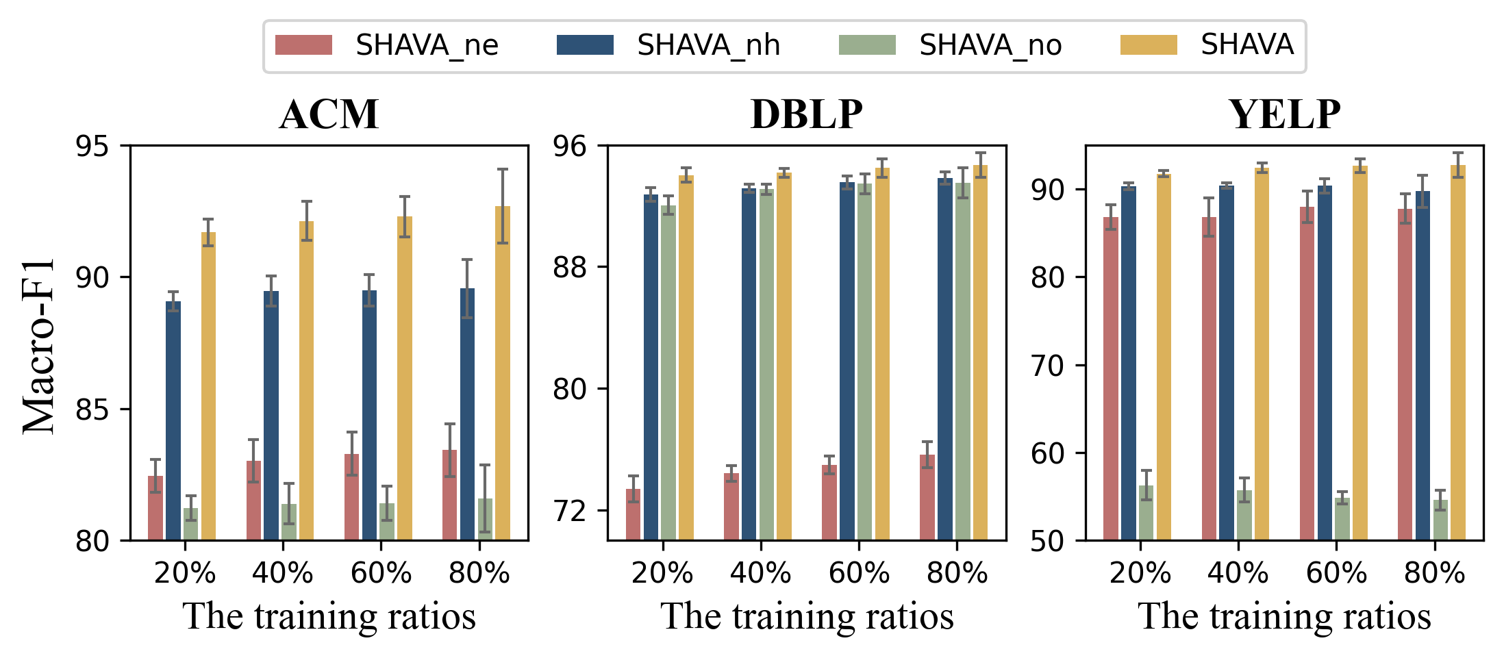
Figure 2. The ablation study results on three datasets.

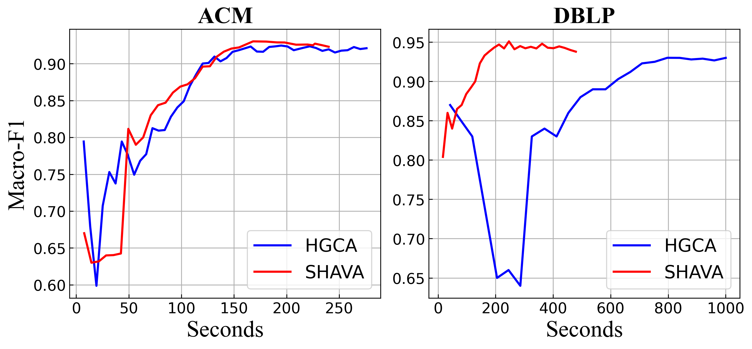
Figure 3. The results of efficiency study.

5.5. Efficiency Study

We next evaluate the efficiency of SHAVA. To ensure a fair comparison, we measure the training time of both SHAVA and HGCA (He et al., 2022). It’s noteworthy that both models are self-supervised, which are specially designed for HINs with missing attributes. We take ACM and DBLP as examples. For illustration, we utilize 80% of labeled nodes as our training set. Figure 3 depicts the changes in Macro-F1 scores of both models as the training time increases. From the figure, we see that SHAVA converges fast and demonstrates consistent performance growth on both datasets. In particular, on DBLP, SHAVA achieves almost $4\times$ speedup than HGCA. This further shows that SHAVA is not only effective but efficient.

5.6. Hyper-parameter Sensitivity Analysis

We end this section with a sensitivity analysis on the hyper-parameters of SHAVA, i.e., the two balance coefficients $\lambda_{1}$ and $\lambda_{2}$. In our experiments, we vary one hyper-parameter each time with the other fixed. Figure 4 shows the Macro-F1 scores for SHAVA on DBLP and YELP. For Micro-F1 scores, we observe similar results, which are thus omitted due to the space limitation. From the figure, we see that for both hyper-parameters, SHAVA can give stable performances over a wide range of values. This demonstrates the insensitivity of SHAVA on hyper-parameters.

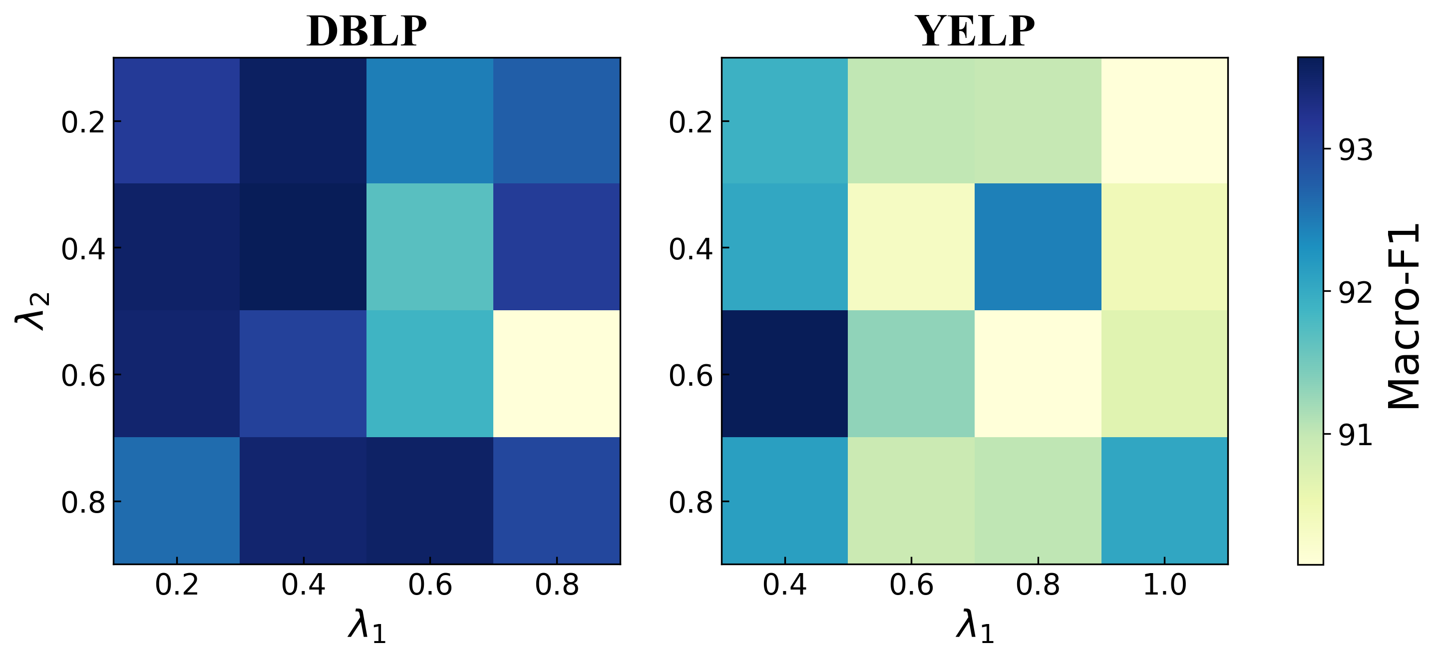
Figure 4. Hyper-parameter sensitivity analysis about $\lambda_{1}$ and $\lambda_{2}$ of node classification on Macro-F1.

6. CONCLUSION

In this paper, we studied generative SSL on heterogeneous graph and proposed SHAVA. Specifically, SHAVA employs variational inference to generate both node-level and attribute-level embeddings. Importantly, SHAVA expand attribute inference in the low-dimensional hidden space to address the problems of missing and inaccurate attributes in HINs. On the one hand, by collaboratively generating node-level and attribute-level embeddings, fine-grained semantic information can be obtained for generating attributes. On the other hand, SHAVA reconstructs the low-dimensional node embedding to alleviate the adverse effect of noise attribute and enhance the feature information of missing attribute. We conducted extensive experiments to evaluate the performance of SHAVA. The results shows that SHAVA is very effective to deal with above problems and lead to superior performance.

Appendix A Datasets

• ACM: This dataset is extracted from the Association for Computing Machinery website (ACM). It contains 4019 papers (P), 7167 authors (A) and 60 subjects (S). The papers are divided into three classes according to the conference they published. In this dataset, only paper’s nodes have original attributes which are bag-of-words representations of their keywords, other nodes have no attribute.

• DBLP: This dataset is extracted from the Association for Computing Machinery website (DBLP). It contains 4057 authors (A), 14328 papers (P), 8789 terms (T) and 20 venues (V). Authors are divided into four research areas according to the conferences they submitted. In this dataset, only paper’s nodes have directly original attributes which are bag-of-words representations of their keywords, other nodes have no attribute.

• YELP: This dataset is extracted from the Yelp Open dataset. It contains 2614 bussinesses (B), 1286 users (U), 4 services (S) and 9 rating levels (L). The business are divided into three classes according to their categories. In this dataset, only bussiness’s node have original attributes which are representations about their descriptions, other nodes have no attribute.

• AMiner: This dataset is extracted from the AMiner citation network. It contains 6564 papers (P), 13329 authors (A) and 35890 reference (R). The papers are divided into four classes. In this dataset, all types of nodes have no attribute.

Table 5. Statistics of datasets.

Datasets	Nodes	Edges	Attributes
ACM	paper(P):4019 author(A):7167 subject(S):60	P-P:9615 P-A:13407 P-S:4019	P:raw A:handcrafted S:handcrafted
DBLP	author(A):4057 paper(P):14328 term(T):7723 venue(V):20	P-A:19645 P-T:85810 P-V:14328	A:handcrafted P:raw T:handcrafted V:handcrafted
YELP	business(B):2614 user(U):1286 service(S):4 level(L):9	B-U:30838 B-S:2614 B-L:2614	B:raw U:handcrafted S:handcrafted L:handcrafted
AMiner	paper(P): 6564 author(A): 13329 reference(R): 35890	P-A: 18007 P-R: 58831	P: handcrafted A: handcrafted S: handcrafted

Appendix B Baselines

• Link prediction. To verify the validity of our model on multiple tasks, we conducted a link prediction experiment. Considering most of HIN models are perform link prediction on virtual neighbors based on meta-paths which are not real links for heterogeneous graph, we conduct link prediction on real edges based on relation. Thus we compare SHAVA  with four homogeneous methods, i.e., VGAE (Kipf and Welling, 2016b), SIG-VAE (Hasanzadeh et al., 2019), CAN (Meng et al., 2019), SeeGera (Li et al., 2023), and three heterogeneous methods which can encoding all type nodes, i.e., RGCN (Schlichtkrull et al., 2018), HGT (Hu et al., 2020).

• Node classification. To further verify the performance of SHAVA, we learned embeddings to the node classification task. We compare SHAVA  with three semi-supervised models, i.e., GAT (Veličković et al., 2017), HAN (Wang et al., 2019a), MAGNN (Fu et al., 2020) and six unsupervised models, i.e., Mp2vec (Dong et al., 2017), DGI (Veličković et al., 2018), DMGI (Park et al., 2020), SeeGera (Li et al., 2023), HGMAE (Tian et al., 2022), HGCA (He et al., 2022).

Table 6. Link prediction results (%). The error bar (±) denotes the standard deviation of the results over five trials. We highlight the best score on each dataset in bold and underline the runner-up results.

Metric	Dataset	Relation	VGAE	SIG-VAE	SeeGera	CAN	RGCN	HGT	SHAVA
AUC	ACM	P-A	$90.87\pm 1.42$	$\underline{92.35\pm 0.79}$	$\textbf{92.86}\pm\textbf{0.41}$	$91.47\pm 0.26$	$78.29\pm 0.72$	$77.83\pm 0.11$	$90.32\pm 0.39$
		P-S	$90.96\pm 2.21$	$89.95\pm 0.46$	$90.23\pm 0.54$	$\underline{95.35\pm 0.24}$	$86.07\pm 4.94$	$91.40\pm 2.91$	$\textbf{96.10}\pm\textbf{ 0.35}$
	DBLP	P-A	$\underline{91.61\pm 0.61}$	$89.34\pm 0.30$	$89.10\pm 1.27$	$89.50\pm 0.41$	$76.48\pm 0.98$	$85.02\pm 2.24$	$\textbf{92.76}\pm\textbf{0.38}$
		P-T	$\underline{91.60\pm 0.33}$	$89.89\pm 0.20$	$90.87\pm 0.16$	$91.26\pm 0.09$	$81.33\pm 1.36$	$88.71\pm 1.17$	$\textbf{92.58}\pm\textbf{0.22}$
		P-V	$92.09\pm 0.49$	$89.15\pm 0.13$	$88.74\pm 0.39$	$94.21\pm 0.32$	$71.66\pm 2.59$	$\underline{96.11\pm 1.43}$	$\textbf{96.35}\pm\textbf{0.18}$
	YELP	B-U	$90.65\pm 0.14$	$88.96\pm 0.95$	$91.05\pm 1.06$	$90.40\pm 0.72$	$91.62\pm 0.41$	$\underline{92.54\pm 0.21}$	$\textbf{93.61}\pm\textbf{0.14}$
		B-S	$84.52\pm 0.74$	$86.45\pm 0.26$	$89.23\pm 0.72$	$92.18\pm 0.08$	$78.27\pm 1.92$	$\underline{97.66}\pm\underline{0.80}$	$\textbf{97.78}\pm\textbf{0.22}$
		B-L	$86.18\pm 0.59$	$85.91\pm 0.05$	$85.89\pm 0.51$	$86.46\pm 0.26$	$84.83\pm 0.28$	$\underline{90.80\pm 1.83}$	$\textbf{91.43}\pm\textbf{0.16}$
AP	ACM	P-A	$\underline{92.40\pm 0.44}$	$\textbf{93.23}\pm\textbf{0.71}$	$92.12\pm 0.40$	$91.93\pm 0.24$	$72.81\pm 0.61$	$73.27\pm 0.93$	$91.06\pm 0.421$
		P-S	$91.95\pm 0.21$	$91.38\pm 0.92$	$91.64\pm 0.47$	$\underline{93.28\pm 0.39}$	$86.47\pm 5.34$	$87.80\pm 3.95$	$\textbf{95.65}\pm\textbf{0.22}$
	DBLP	P-A	$\underline{91.20\pm 0.85}$	$87.87\pm 0.53$	$88.37\pm 0.73$	$87.83\pm 0.55$	$66.93\pm 0.51$	$80.64\pm 0.82$	$\textbf{92.34}\pm\textbf{0.48}$
		P-T	$\underline{92.37\pm 0.29}$	$91.75\pm 0.19$	$90.96\pm 0.06$	$91.54\pm 0.07$	$85.02\pm 0.59$	$87.31\pm 1.73$	$\textbf{92.92}\pm\textbf{0.18}$
		P-V	$93.62\pm 0.55$	$91.14\pm 0.10$	$90.97\pm 0.37$	$94.91\pm 0.29$	$60.51\pm 0.11$	$\underline{95.09\pm 1.72}$	$\textbf{95.70}\pm\textbf{0.17}$
	YELP	B-U	$89.97\pm 0.38$	$88.02\pm 0.77$	$90.09\pm 1.64$	$88.64\pm 0.52$	$\underline{91.05\pm 0.37}$	$90.71\pm 0.32$	$\textbf{92.65}\pm\textbf{0.04}$
		B-S	$83.85\pm 1.81$	$88.29\pm 0.69$	$91.72\pm 0.41$	$93.32\pm 0.80$	$81.28\pm 0.49$	$\underline{97.34\pm 1.41}$	$\textbf{97.52}\pm\textbf{0.28}$
		B-L	$85.75\pm 0.19$	$83.21\pm 0.17$	$83.50\pm 0.77$	$\underline{86.84\pm 0.61}$	$81.28\pm 0.48$	$85.85\pm 2.16$	$\textbf{88.58}\pm\textbf{0.97}$

Appendix C Implementation Details

We have implemented SHAVA using PyTorch. The model is initialized with Xavier initialization (Glorot and Bengio, 2010) and trained using the Adam optimizer (Kingma and Ba, 2014). For homogeneous methods, we treat all nodes and edges as the same type. We fine-tune the hyper-parameters for all methods we have compared to report their best results. For SHAVA, we use the two-layer simple HGNN mentioned above as the backbone for the encoder. For other hyperparameters, we conduct a grid search. The learning rate is adjusted within {0.001, 0.005, 0.01, 0.05}, and the dropout rate is selected from {0.0, 0.3}. Additionally, we utilize multi-head attention with the number of attention heads K from {1, 2, 4, 8}. The embedding dimension is searched from the range {32, 64, 128, 256}. For hyperparameters $\lambda_{1}$ and $\lambda_{2}$, we select values from the range [0, 1] with a step of 0.1. The number of HGNN layers we use for decoding is selected from {0, 1, 2}. For fairness, we run all the experiments on a server with 32G memory and a single Tesla V100 GPU.

Appendix D Link Prediction

For the link prediction task, we treat the connected nodes in the HIN as positive node pairs, and use other unconnected nodes as negative node pairs. We perform experiments separately for each edge type. To predict each edge type based on relation, we divide the positive node pairs into training set, validation set and testing set according to 85%, 5% and 10% respectively, and randomly select the same number of negative node pairs to add to the partitioned dataset. Meanwhile, we retain all edges of other types when predicting one edge type. We use two metrics AUC (Area Under the Curve) and AP (Average Precision) to evaluate model performance. The larger their values, the better the model performance. We select hyper-parameters with a patience of 100 by validation set. For all methods, we run experiments 5 times with different random seeds and report the mean and standard deviation of them, as shown in table 6.

From the table, we have the following observations: (1) SHAVA consistently outperforms the competitive methods across various relationships in the majority of datasets, which indicates the superiority of SHAVA for the link prediction task in HINs. (2) The homogeneous methods SeeGera and SIG-VAE achieve the best performance on the P-A relationship of ACM dataset, respectively. The homogeneous methods treat all nodes and relationships on heterogeneous graph construction as the same type. Therefore, while these methods achieve the best results on certain relationships on heterogeneous graphs, they evidently cannot simultaneously consider all relationships. In comparison, SHAVA has achieved the best results across all relationships in most datasets. All these results show the effectiveness of SHAVA on heterogeneous graphs.

Appendix E Variational Lower Bound

According to SIVI, the adjacency matrix $\mathrm{A}$ and the attribute matrix $\mathrm{X}$ are observed of the heterogenous graph, in order to approximate the true posterior distribution $p(\mathrm{Z}^{\mathcal{V}},\mathrm{Z}^{\mathcal{A}}|\mathrm{A},\mathrm{X})$, considering the SIVI we need a variational distribution $h_{\phi}(\mathrm{Z}^{\mathcal{V}},\mathrm{Z}^{\mathcal{A}})$ with a variational parameter $\psi$ to minimize $\text{KL}(h_{\phi}(\mathrm{Z}^{\mathcal{V}},\mathrm{Z}^{\mathcal{A}})||p(\mathrm{Z}^{\mathcal{V}},\mathrm{Z}^{\mathcal{A}}|\mathrm{A},\mathrm{X}))$, which is equivalent to maximizing the ELBO (Bishop and Tipping, 2013):

(A.1) $$\text{ELBO}=\mathrm{E}_{\mathrm{Z}^{\mathcal{V}},\mathrm{Z}^{\mathcal{A}}\sim h_{\phi}(\mathrm{Z}^{\mathcal{V}},\mathrm{Z}^{\mathcal{A}})}[\log\frac{p(\mathrm{Z}^{\mathcal{V}},\mathrm{Z}^{\mathcal{A}},\mathrm{A},\mathrm{X})}{h_{\phi}(\mathrm{Z}^{\mathcal{V}},\mathrm{Z}^{\mathcal{A}})}]=\mathcal{L}.$$

Since $\mathrm{Z}^{\mathcal{V}}$ and $\mathrm{Z}^{\mathcal{A}}$ represent node-level and attribute-level respectively, we assume that they are independent and come from different variational distributions:

(A.2) $$\mathrm{Z}^{\mathcal{V}}\sim h_{\phi_{1}}(\mathrm{Z}^{\mathcal{V}})=\int_{\psi_{1}}q_{1}(\mathrm{Z}^{\mathcal{V}}\mid\psi_{1})q_{\phi_{1}}(\psi_{1})\mathrm{d}\psi_{1},$$

$$\mathrm{Z}^{\mathcal{A}}\sim h_{\phi_{2}}(\mathrm{Z}^{\mathcal{A}})=\int_{\psi_{2}}q_{2}(\mathrm{Z}^{\mathcal{A}}\mid\psi_{2})q_{\phi_{2}}(\psi_{2})\mathrm{d}\psi_{2}.$$

Thereby, the $h_{\phi}(\mathrm{Z}^{\mathcal{V}},\mathrm{Z}^{\mathcal{A}})$ is a mean-field distribution that can be factorized as:

(A.3) $$h_{\phi}(\mathrm{Z}^{\mathcal{V}},\mathrm{Z}^{\mathcal{A}})=h_{\phi_{1}}(\mathrm{Z}^{\mathcal{V}})h_{\phi_{2}}(\mathrm{Z}^{\mathcal{A}}).$$

The joint distribution $p(\mathrm{Z}^{\mathcal{V}},\mathrm{Z}^{\mathcal{A}},\mathrm{A},\mathrm{X})$ can be represented as:

(A.4) $$p(\mathrm{Z}^{\mathcal{V}},\mathrm{Z}^{\mathcal{A}},\mathrm{A},\mathrm{X})=p(\mathrm{Z}^{\mathcal{V}})p(\mathrm{Z}^{\mathcal{A}})p(\mathrm{A}|\mathrm{Z}^{\mathcal{V}})p(\mathrm{X}|\mathrm{Z}^{\mathcal{V}},\mathrm{Z}^{\mathcal{A}}).$$

Due to the concavity of the logarithmic function, we use Jensen’s inequality to derive a lower bound for the ELBO by substituting (A.3) and (A.4) into (A.1):

(A.5) $$\mathcal{L} =\mathrm{E}_{\mathrm{Z}^{\mathcal{V}}\sim{h_{\phi_{1}}(\mathrm{Z}^{\mathcal{V}}),\mathrm{Z}^{\mathcal{A}}\sim h_{\phi_{2}}(\mathrm{Z}^{\mathcal{A}})}}$$

$$\left[\log\frac{p(\mathrm{Z}^{\mathcal{V}})p(\mathrm{Z}^{\mathcal{A}})p(\mathrm{A}|\mathrm{Z}^{\mathcal{V}})p(\mathrm{X}|\mathrm{Z}^{\mathcal{V}},\mathrm{Z}^{\mathcal{A}})}{h_{\phi_{1}}(\mathrm{Z}^{\mathcal{V}})h_{\phi_{2}}(\mathrm{Z}^{\mathcal{A}})}\right]$$

$$\geq\mathrm{E}_{\mathrm{Z}^{\mathcal{V}}\sim{h_{\phi_{1}}(\mathrm{Z}^{\mathcal{V}})}}\log p(\mathrm{A}|\mathrm{Z}^{\mathcal{V}})$$

$$+\mathrm{E}_{\mathrm{Z}^{\mathcal{V}}\sim{h_{\phi_{1}}(\mathrm{Z}^{\mathcal{V}}),\mathrm{Z}^{A}\sim h_{\phi_{2}}(\mathrm{Z}^{\mathcal{A}})}}\log p(\mathrm{X}|\mathrm{Z}^{\mathcal{V}},\mathrm{Z}^{\mathcal{A}})$$

$$+\mathrm{E}_{\mathrm{Z}^{\mathcal{V}}\sim{h_{\phi_{1}}(\mathrm{Z}^{\mathcal{V}})}}\left[\log\frac{p(\mathrm{Z}^{\mathcal{V}})}{h_{\phi_{1}}(\mathrm{Z}^{\mathcal{V}})}\right]$$

$$+\mathrm{E}_{\mathrm{Z}^{\mathcal{A}}\sim h_{\phi_{2}}(\mathrm{Z}^{\mathcal{A}})}\left[\log\frac{p(\mathrm{Z}^{\mathcal{A}})}{h_{\phi_{2}}(\mathrm{Z}^{\mathcal{A}})}\right]$$

$$=\mathrm{E}_{\mathrm{Z}^{\mathcal{V}}\sim{h_{\phi_{1}}(\mathrm{Z}^{\mathcal{V}})}}\log p(\mathrm{A}|\mathrm{Z}^{\mathcal{V}})$$

$$+\mathrm{E}_{\mathrm{Z}^{\mathcal{V}}\sim{h_{\phi_{1}}(\mathrm{Z}^{\mathcal{V}}),\mathrm{Z}^{\mathcal{A}}\sim h_{\phi_{2}}(\mathrm{Z}^{\mathcal{A}})}}\log p(\mathrm{X}|\mathrm{Z}^{\mathcal{V}},\mathrm{Z}^{\mathcal{A}})$$

$$-\text{KL}(h_{\phi_{1}}(\mathrm{Z}^{\mathcal{V}})||p(\mathrm{Z}^{\mathcal{V}}))-\text{KL}(h_{\phi_{2}}(\mathrm{Z}^{\mathcal{A}})||p(\mathrm{Z}^{\mathcal{A}}))$$

$$=\underline{\mathcal{L}}.$$

where $\underline{\mathcal{L}}$ is the evidence lower bound that satisfies $\log(\mathrm{A},\mathrm{X})\geq\underline{\mathcal{L}}$, $\text{KL}(p(\cdot)\ ||\ q(\cdot))$ is the Kullback-Leibler deivergence that compare the difference between probability distribution $p$ and $q$, $h_{\phi_{1}}(\mathrm{Z}^{\mathcal{V}})$ and $h_{\phi_{2}}(\mathrm{Z}^{\mathcal{A}})$ are variational posterior distributions generated from the node encoder and the attribute encoder respectively. By sampling latent embeddings $\mathrm{Z}^{V}$ and $\mathrm{Z}^{A}$ from $h_{\phi_{1}}(\mathrm{Z}^{V})$ and $h_{\phi_{2}}(\mathrm{Z}^{A})$ and inputing into decoder , $p(\mathrm{A}|\mathrm{Z}^{\mathcal{V}})$ and $p(\mathrm{X}|\mathrm{Z}^{\mathcal{V}},\mathrm{Z}^{\mathcal{A}})$ obtained by decoder should be close to observed data .

Generally, maximizing the $\underline{\mathcal{L}}$, we need to consider the reconstruction loss and the KL divergence.

References

- (1)
- Berg et al. (2017) Rianne van den Berg, Thomas N Kipf, and Max Welling. 2017. Graph convolutional matrix completion. arXiv preprint arXiv:1706.02263 (2017).
- Bishop and Tipping (2013) Christopher M Bishop and Michael Tipping. 2013. Variational relevance vector machines. arXiv preprint arXiv:1301.3838 (2013).
- Busbridge et al. (2019) Dan Busbridge, Dane Sherburn, Pietro Cavallo, and Nils Y Hammerla. 2019. Relational graph attention networks. arXiv preprint arXiv:1904.05811 (2019).
- Chen et al. (2023) Shuyi Chen, Kaize Ding, and Shixiang Zhu. 2023. Uncertainty-Aware Robust Learning on Noisy Graphs. arXiv preprint arXiv:2306.08210 (2023).
- Dong et al. (2017) Yuxiao Dong, Nitesh V Chawla, and Ananthram Swami. 2017. metapath2vec: Scalable representation learning for heterogeneous networks. In KDD. 135–144.
- Dong et al. (2020) Yuxiao Dong, Ziniu Hu, Kuansan Wang, Yizhou Sun, and Jie Tang. 2020. Heterogeneous Network Representation Learning.. In IJCAI, Vol. 20. 4861–4867.
- Fu et al. (2020) Xinyu Fu, Jiani Zhang, Ziqiao Meng, and Irwin King. 2020. Magnn: Metapath aggregated graph neural network for heterogeneous graph embedding. In WebConf. 2331–2341.
- Glorot and Bengio (2010) Xavier Glorot and Yoshua Bengio. 2010. Understanding the difficulty of training deep feedforward neural networks. In Proceedings of the thirteenth international conference on artificial intelligence and statistics. JMLR Workshop and Conference Proceedings, 249–256.
- Hamilton et al. (2017) Will Hamilton, Zhitao Ying, and Jure Leskovec. 2017. Inductive representation learning on large graphs. NeurIPS 30 (2017).
- Hasanzadeh et al. (2019) Arman Hasanzadeh, Ehsan Hajiramezanali, Krishna Narayanan, Nick Duffield, Mingyuan Zhou, and Xiaoning Qian. 2019. Semi-implicit graph variational auto-encoders. NeurIPS 32 (2019).
- He et al. (2022) Dongxiao He, Chundong Liang, Cuiying Huo, Zhiyong Feng, Di Jin, Liang Yang, and Weixiong Zhang. 2022. Analyzing heterogeneous networks with missing attributes by unsupervised contrastive learning. IEEE Transactions on Neural Networks and Learning Systems (2022).
- Hou et al. (2022) Zhenyu Hou, Xiao Liu, Yukuo Cen, Yuxiao Dong, Hongxia Yang, Chunjie Wang, and Jie Tang. 2022. Graphmae: Self-supervised masked graph autoencoders. In Proceedings of the 28th ACM SIGKDD Conference on Knowledge Discovery and Data Mining. 594–604.
- Hu et al. (2019) Binbin Hu, Yuan Fang, and Chuan Shi. 2019. Adversarial learning on heterogeneous information networks. In KDD. 120–129.
- Hu et al. (2020) Ziniu Hu, Yuxiao Dong, Kuansan Wang, and Yizhou Sun. 2020. Heterogeneous graph transformer. In WebConf. 2704–2710.
- Jin et al. (2021) Di Jin, Cuiying Huo, Chundong Liang, and Liang Yang. 2021. Heterogeneous graph neural network via attribute completion. In Proceedings of the Web Conference 2021. 391–400.
- Kingma and Ba (2014) Diederik P Kingma and Jimmy Ba. 2014. Adam: A method for stochastic optimization. arXiv preprint arXiv:1412.6980 (2014).
- Kipf and Welling (2016a) Thomas N Kipf and Max Welling. 2016a. Semi-supervised classification with graph convolutional networks. arXiv preprint arXiv:1609.02907 (2016).
- Kipf and Welling (2016b) Thomas N Kipf and Max Welling. 2016b. Variational graph auto-encoders. arXiv preprint arXiv:1611.07308 (2016).
- Li et al. (2021) Xiang Li, Danhao Ding, Ben Kao, Yizhou Sun, and Nikos Mamoulis. 2021. Leveraging meta-path contexts for classification in heterogeneous information networks. In ICDE. 912–923.
- Li et al. (2023) Xiang Li, Tiandi Ye, Caihua Shan, Dongsheng Li, and Ming Gao. 2023. SeeGera: Self-supervised Semi-implicit Graph Variational Auto-encoders with Masking. In WebConf. 143–153.
- Liu et al. (2022) Yixin Liu, Ming Jin, Shirui Pan, Chuan Zhou, Yu Zheng, Feng Xia, and S Yu Philip. 2022. Graph self-supervised learning: A survey. IEEE TKDE 35, 6 (2022), 5879–5900.
- Lu et al. (2019) Yuanfu Lu, Chuan Shi, Linmei Hu, and Zhiyuan Liu. 2019. Relation structure-aware heterogeneous information network embedding. In AAAI, Vol. 33. 4456–4463.
- Mao et al. (2023) Qiheng Mao, Zemin Liu, Chenghao Liu, and Jianling Sun. 2023. Hinormer: Representation learning on heterogeneous information networks with graph transformer. In WebConf. 599–610.
- Meng et al. (2019) Zaiqiao Meng, Shangsong Liang, Hongyan Bao, and Xiangliang Zhang. 2019. Co-embedding attributed networks. In WSDM. 393–401.
- Pan et al. (2018) Shirui Pan, Ruiqi Hu, Guodong Long, Jing Jiang, Lina Yao, and Chengqi Zhang. 2018. Adversarially regularized graph autoencoder for graph embedding. arXiv preprint arXiv:1802.04407 (2018).
- Park et al. (2020) Chanyoung Park, Jiawei Han, and Hwanjo Yu. 2020. Deep multiplex graph infomax: Attentive multiplex network embedding using global information. Knowledge-Based Systems 197 (2020), 105861.
- Rossi et al. (2022) Emanuele Rossi, Henry Kenlay, Maria I Gorinova, Benjamin Paul Chamberlain, Xiaowen Dong, and Michael M Bronstein. 2022. On the unreasonable effectiveness of feature propagation in learning on graphs with missing node features. In Learning on Graphs Conference. PMLR, 11–1.
- Salehi and Davulcu (2019) Amin Salehi and Hasan Davulcu. 2019. Graph attention auto-encoders. arXiv preprint arXiv:1905.10715 (2019).
- Schlichtkrull et al. (2018) Michael Schlichtkrull, Thomas N Kipf, Peter Bloem, Rianne Van Den Berg, Ivan Titov, and Max Welling. 2018. Modeling relational data with graph convolutional networks. In The Semantic Web: 15th International Conference, ESWC 2018, Heraklion, Crete, Greece, June 3–7, 2018, Proceedings 15. Springer, 593–607.
- Shi et al. (2016) Chuan Shi, Yitong Li, Jiawei Zhang, Yizhou Sun, and S Yu Philip. 2016. A survey of heterogeneous information network analysis. TKDE 29, 1 (2016), 17–37.
- Sun et al. (2019b) Fan-Yun Sun, Jordan Hoffmann, Vikas Verma, and Jian Tang. 2019b. Infograph: Unsupervised and semi-supervised graph-level representation learning via mutual information maximization. arXiv preprint arXiv:1908.01000 (2019).
- Sun (2012) Yizhou Sun. 2012. Mining heterogeneous information networks. University of Illinois at Urbana-Champaign.
- Sun et al. (2011) Yizhou Sun, Jiawei Han, Xifeng Yan, Philip S Yu, and Tianyi Wu. 2011. Pathsim: Meta path-based top-k similarity search in heterogeneous information networks. Proceedings of the VLDB Endowment 4, 11 (2011), 992–1003.
- Sun et al. (2013) Yizhou Sun, Brandon Norick, Jiawei Han, Xifeng Yan, Philip S Yu, and Xiao Yu. 2013. Pathselclus: Integrating meta-path selection with user-guided object clustering in heterogeneous information networks. ACM TKDD 7, 3 (2013), 1–23.
- Sun et al. (2019a) Zhiqing Sun, Zhi-Hong Deng, Jian-Yun Nie, and Jian Tang. 2019a. Rotate: Knowledge graph embedding by relational rotation in complex space. arXiv preprint arXiv:1902.10197 (2019).
- Taguchi et al. (2021) Hibiki Taguchi, Xin Liu, and Tsuyoshi Murata. 2021. Graph convolutional networks for graphs containing missing features. Future Generation Computer Systems 117 (2021), 155–168.
- Tian et al. (2022) Yijun Tian, Kaiwen Dong, Chunhui Zhang, Chuxu Zhang, and Nitesh V Chawla. 2022. Heterogeneous Graph Masked Autoencoders. arXiv preprint arXiv:2208.09957 (2022).
- Veličković et al. (2017) Petar Veličković, Guillem Cucurull, Arantxa Casanova, Adriana Romero, Pietro Lio, and Yoshua Bengio. 2017. Graph attention networks. arXiv preprint arXiv:1710.10903 (2017).
- Veličković et al. (2018) Petar Veličković, William Fedus, William L Hamilton, Pietro Liò, Yoshua Bengio, and R Devon Hjelm. 2018. Deep graph infomax. arXiv preprint arXiv:1809.10341 (2018).
- Velickovic et al. (2019) Petar Velickovic, William Fedus, William L Hamilton, Pietro Liò, Yoshua Bengio, and R Devon Hjelm. 2019. Deep graph infomax. ICLR (Poster) 2, 3 (2019), 4.
- Wang et al. (2016) Daixin Wang, Peng Cui, and Wenwu Zhu. 2016. Structural deep network embedding. In KDD. 1225–1234.
- Wang et al. (2021b) Wei Wang, Xiangyu Wei, Xiaoyang Suo, Bin Wang, Hao Wang, Hong-Ning Dai, and Xiangliang Zhang. 2021b. Hgate: heterogeneous graph attention auto-encoders. TKDE (2021).
- Wang et al. (2019a) Xiao Wang, Houye Ji, Chuan Shi, Bai Wang, Yanfang Ye, Peng Cui, and Philip S Yu. 2019a. Heterogeneous graph attention network. In WebConf. 2022–2032.
- Wang et al. (2021a) Xiao Wang, Nian Liu, Hui Han, and Chuan Shi. 2021a. Self-supervised heterogeneous graph neural network with co-contrastive learning. In Proceedings of the 27th ACM SIGKDD conference on knowledge discovery & data mining. 1726–1736.
- Wang et al. (2019b) Xiaoyun Wang, Xuanqing Liu, and Cho-Jui Hsieh. 2019b. Graphdefense: Towards robust graph convolutional networks. arXiv preprint arXiv:1911.04429 (2019).
- Wu et al. (2021) Lirong Wu, Haitao Lin, Cheng Tan, Zhangyang Gao, and Stan Z Li. 2021. Self-supervised learning on graphs: Contrastive, generative, or predictive. IEEE Transactions on Knowledge and Data Engineering (2021).
- Xu et al. (2022) Zhe Xu, Boxin Du, and Hanghang Tong. 2022. Graph sanitation with application to node classification. In WebConf. 1136–1147.
- Yang et al. (2023) Xiaocheng Yang, Mingyu Yan, Shirui Pan, Xiaochun Ye, and Dongrui Fan. 2023. Simple and efficient heterogeneous graph neural network. In AAAI, Vol. 37. 10816–10824.
- Yin and Zhou (2018) Mingzhang Yin and Mingyuan Zhou. 2018. Semi-implicit variational inference. In ICML. PMLR, 5660–5669.
- You et al. (2020b) Jiaxuan You, Xiaobai Ma, Yi Ding, Mykel J Kochenderfer, and Jure Leskovec. 2020b. Handling missing data with graph representation learning. NeurIPS 33 (2020), 19075–19087.
- You et al. (2020a) Yuning You, Tianlong Chen, Yongduo Sui, Ting Chen, Zhangyang Wang, and Yang Shen. 2020a. Graph contrastive learning with augmentations. NeurIPS 33 (2020), 5812–5823.
- Yun et al. (2019) Seongjun Yun, Minbyul Jeong, Raehyun Kim, Jaewoo Kang, and Hyunwoo J Kim. 2019. Graph transformer networks. NeurIPS 32 (2019).
- Zhang et al. (2019b) Chuxu Zhang, Dongjin Song, Chao Huang, Ananthram Swami, and Nitesh V Chawla. 2019b. Heterogeneous graph neural network. In KDD. 793–803.
- Zhang et al. (2019a) Jiani Zhang, Xingjian Shi, Shenglin Zhao, and Irwin King. 2019a. Star-gcn: Stacked and reconstructed graph convolutional networks for recommender systems. arXiv preprint arXiv:1905.13129 (2019).
- Zhu et al. (2023) Guanghui Zhu, Zhennan Zhu, Wenjie Wang, Zhuoer Xu, Chunfeng Yuan, and Yihua Huang. 2023. AutoAC: Towards Automated Attribute Completion for Heterogeneous Graph Neural Network. arXiv preprint arXiv:2301.03049 (2023).
- Zhu et al. (2021) Yanqiao Zhu, Yichen Xu, Feng Yu, Qiang Liu, Shu Wu, and Liang Wang. 2021. Graph contrastive learning with adaptive augmentation. In Proceedings of the Web Conference 2021. 2069–2080.
- Zügner et al. (2020) Daniel Zügner, Oliver Borchert, Amir Akbarnejad, and Stephan Günnemann. 2020. Adversarial attacks on graph neural networks: Perturbations and their patterns. ACM TKDD 14, 5 (2020), 1–31.