Non-Hermitian topological wall modes in rotating Rayleigh–Bénard convection

Abstract

We show that the rotating Rayleigh–Bénard convection, where a rotating fluid is heated from below, exhibits non-Hermitian topological states. Recently, Favier & Knobloch (2020) hypothesized that the robust wall modes in rapidly rotating convection are topologically protected. We study the linear problem around the conduction profile, and by considering a Berry curvature defined in the complex wavenumber space, particularly, by introducing a complex vertical wavenumber, we find that these modes can be characterized by a non-zero integer Chern number, indicating their topological nature. The eigenvalue problem is intrinsically non-Hermitian, therefore the definition of Berry curvature generalizes that of the stably stratified problem. Moreover, the three-dimensional setup naturally regularizes the eigenvector at the infinite horizontal wavenumber. Under the hydrostatic approximation, it recovers a two-dimensional analogue of the one which explains the topological origin of the equatorial Kelvin and Yanai waves (Delplace et al., 2017). The existence of the tenacious wall modes relies only on rotation when the fluid is stratified, no matter whether it is stable or unstable. However, the neutrally stratified system does not support a topological edge state. In addition, we define a winding number to visualize the topological nature of the fluid.

1 Introduction

Rotating Rayleigh-Bénard convection, where rotating fluid between two horizontal plates is driven by bottom heating, is an important prototype for geophysics and astrophysics (Bodenschatz et al., 2000; Ahlers et al., 2009; King et al., 2012; Guervilly et al., 2014). It occurs in various natural systems, such as the Earth’s atmosphere and oceans, as well as in the interiors of stars and exoplanets.

In this convection system, the rotation leads to the emergence of edge states at the sidewall (Zhong et al., 1991, 1993; Ecke et al., 1992; Goldstein et al., 1993; Ning & Ecke, 1993), which are characterized by their unidirectional propagation and their ability to persist even in the presence of different types of barriers and turbulence (Favier & Knobloch, 2020; Ecke, 2023; Ecke & Shishkina, 2023). These states were first discovered through experiments indirectly by Rossby (1969), where a surprising convection occurs with a Rayleigh number ($R_{a}$) below the critical value for the laterally unbounded system (Chandrasekhar, 1961). Zhang & Liao (2009) gives the asymptotic expression of the critical $R_{a}$ for the onset of these wall modes, regaining the leading terms previously calculated by Herrmann & Busse (1993). With increasing $R_{a}$, more wall modes emerge, and they may undergo modulational instabilities and interact with bulk modes, resulting in complex nonlinear dynamics (Zhong et al., 1993; Liu & Ecke, 1999; Horn & Schmid, 2017). In the turbulent flows with high $R_{a}$, the wall modes may be transformed to the boundary zonal flows, which can also coexist with bulk convection (Zhang et al., 2020; de Wit et al., 2020; Ecke et al., 2022). Beyond these detailed studies, a new insight is proposed that these edge states may be related to the topological nature of the system (Favier & Knobloch, 2020). Thus, a new set of questions arises, such as, can we obtain the topological invariant of the system? How robust in quantitative terms is the topology in the presence of turbulence? The answers to these follow-up questions will deepen our understanding of the overall flow structure and the spatial distribution of heat flux in geophysical and astrophysical contexts (Zhong et al., 2009; Terrien et al., 2023).

Edge states under topological protection have been a topic of great interest in recent years. These edge states are robust against disorder and perturbations, and their topological protection originates from the nontrivial topology of the underlying bulk system. This topological nature can be indicated by a corresponding topological invariant, such as the Chern number (Xiao et al., 2010; Delplace et al., 2017) or the winding number (Zhu et al., 2023). When the topological invariant is non-zero, the bulk-boundary correspondence guarantees the existence of robust edge states (Essin & Gurarie, 2011; Venaille et al., 2023). The topological physics first appeared in condensed matters (Kosterlitz & Thouless, 1973; Thouless et al., 1982; Haldane, 1988), such as topological insulators (Hasan & Kane, 2010), topological photonics (Ozawa et al., 2019) and topological phononics (Liu et al., 2020). Recently similar topological properties have been found in macroscopic systems, especially in hydrodynamics, such as the topological origin of trapped waves near the equator or coastlines (Delplace et al., 2017; Venaille & Delplace, 2021), the topological waves in fluids with odd viscosity (Souslov et al., 2019), and the presence of topological invariants in active matter systems (Shankar et al., 2022). This universality of topological states can be attributed to the similar symmetries embodied in the systems of different scales (Senthil, 2015).

In this paper, we point out that the linearized rotating convection is a non-Hermitian system and that these edge states are manifestations of the nontrivial topological Berry phase in the bulk. Non-Hermitian systems are open systems that do not obey the Hermitian symmetry property (Ashida et al., 2020). Thus, their eigenvalues are not necessarily real, and the corresponding eigenvectors can be unorthogonal. Rayleigh-Bénard convection is non-Hermitian because it exchanges energy with an external heat source. Non-Hermitian systems exhibit unconventional physical properties, including non-reciprocal transmission, exceptional points, and topological phase transitions (Bergholtz et al., 2021; Ding et al., 2022). These phenomena have attracted significant attention in recent years due to their potential applications in various fields of physics, such as optics, condensed matter physics, and quantum information science.

With the non-Hermitian and topological nature, we foresee that the rotating convection will become a more abundant system and act as a platform for probing topological states in turbulent flows. This paper is structured as follows. Sec.2.1 introduces the Non-Hermitian Hamiltonian matrix of the linearized governing equations. Sec.2.2 explains the calculation of Chern number in non-Hermitian systems. Sec.3 focuses on calculating the topological invariants in the unstably stratified case. Sec.4 explores the topological properties of the system in stable and critical cases. Sec.5 discusses the calculation of the Chern number under the hydrostatic approximation. Sec.6 visualizes the topological nature through winding numbers. Finally, discussions and summaries are presented in Sec. 7. The appendix Sec. A discusses the solutions satisfying realistic boundary conditions.

2 The non-Hermitian eigenvalue problem of linearized rotating convection

2.1 Non-Hermitian Hamiltonian matrix

The governing equations for the rotating Rayleigh-Bénard convection include the Navier-Stokes, continuity, and temperature equations. The dimensionless form can be written as (cf. Favier & Knobloch, 2020):

$$\frac{\partial\boldsymbol{u}}{\partial t}+\left(\boldsymbol{u}\cdot\boldsymbol{\nabla}\right)\boldsymbol{u} =-\boldsymbol{\nabla}p-\lambda\boldsymbol{e}_{z}\times\boldsymbol{u}+\alpha\theta\boldsymbol{e}_{z}+E\nabla^{2}\boldsymbol{u},$$ (1a)

$$\boldsymbol{\nabla}\cdot\boldsymbol{u} =0,$$ (1b)

$$\frac{\partial\theta}{\partial t}+\left(\boldsymbol{u}\cdot\boldsymbol{\nabla}\right)\theta =w+\frac{E}{Pr}\nabla^{2}\theta,$$ (1c)

where $\boldsymbol{u}=(u,v,w)$ is the velocity vector, $\lambda=\pm 1$ indicates the direction of rotation, $p$ is the pressure, $\theta$ is the temperature fluctuation relative to the linear conduction profile, $\alpha=RaE^{2}/Pr$ is the square of the convective Rossby number. The Rayleigh number is $Ra=\beta g\Delta Th^{3}/\nu\kappa$, where $\beta$ is the thermal expansion coefficient, $g$ is the acceleration due to gravity, $\Delta T$ is the temperature difference between the top and bottom plates, $h$ is the height of the fluid layer, and $\nu$ and $\kappa$ are the viscosity and thermal diffusivity, respectively. It is a measure of the strength of the buoyancy-driven flow relative to the viscous forces. The Ekman number $E=\nu/(2\Omega h^{2})$, describes the balance of viscous forces to Coriolis forces, where $\Omega$ is the angular velocity of rotation. The Prandtl number is $Pr=\nu/\kappa$ and is a measure of the relative importance of viscous and thermal diffusion.

Considering a normal-mode ansatz $(u,v,w,p,\theta)=Re\{(\hat{u},\hat{v},\hat{w},\hat{p},\hat{\theta})e^{i(\boldsymbol{k\cdot r}-\omega t)}\}$ with the wavenumber $\boldsymbol{k}=(k_{x},k_{y},k_{z})$, the linearized equations become

$$-i\omega\boldsymbol{\hat{u}}=-i\hat{p}\boldsymbol{k}-\lambda\boldsymbol{e}_{z}\times\boldsymbol{\hat{u}}+\alpha\hat{\theta}\boldsymbol{e}_{z}-Ek^{2}\boldsymbol{\hat{u}},$$ (2)

$$\boldsymbol{k}\cdot\boldsymbol{\hat{u}}=0,$$ (3)

$$-i\omega\hat{\theta}=\hat{w}-\frac{E}{Pr}k^{2}\hat{\theta},$$ (4)

where $k=\sqrt{k_{x}^{2}+k_{y}^{2}+k_{z}^{2}}$. Taking the divergence of both sides of Eq.(2) and combining with Eq.(3), we get

$$0=\hat{p}k^{2}+i\lambda(k_{x}\hat{v}-k_{y}\hat{u})+i\alpha k_{z}\hat{\theta}.$$ (5)

Then

$$\hat{p}=i\frac{\lambda(-k_{x}\hat{v}+k_{y}\hat{u})-\alpha k_{z}\hat{\theta}}{k^{2}}.$$ (6)

With the wave vector $\psi\equiv(\hat{u},\hat{v},\hat{w},\hat{\theta})$, we get the eigen equation from Eq.(2) and Eq.(4) as

$$H\psi=\omega\psi,$$ (7)

with

$$H=i\left[\begin{array}[]{cccc}E_{0}+\lambda\frac{k_{x}k_{y}}{k^{2}}&\lambda\left(1-\frac{k_{x}^{2}}{k^{2}}\right)&0&-\alpha\frac{k_{x}k_{z}}{k^{2}}\\ \lambda\left(-1+\frac{k_{y}^{2}}{k^{2}}\right)&E_{0}-\lambda\frac{k_{x}k_{y}}{k^{2}}&0&-\alpha\frac{k_{y}k_{z}}{k^{2}}\\ \lambda\frac{k_{y}k_{z}}{k^{2}}&-\lambda\frac{k_{x}k_{z}}{k^{2}}&E_{0}&\alpha-\alpha\frac{k_{z}^{2}}{k^{2}}\\ 0&0&1&E_{1}\end{array}\right],$$ (8)

where $E_{0}=-Ek^{2}$, $E_{1}=E_{0}/Pr$. This is a non-Hermitian Hamiltonian because $H\neq H^{\dagger}$, where $\dagger$ denotes the conjugate transpose. The eigenvalue $\omega$ can take a complex number, unlike in the Hermitian case where $\omega$ is real. The eigenvalue problem of $H^{\dagger}$ is

$$H^{\dagger}\psi^{\prime}=\omega^{\ast}\psi^{\prime},$$ (9)

where $\omega^{\ast}$ is the complex conjugate of $\omega$, and $\psi^{\prime}$ is generally different from $\psi$.

In (1), we do not include the boundary conditions, and the main text of this paper focuses on demonstrating the idea that to calculate a Chern number for rotating convection a complex vertical wavenumber is required. A discussion on realistic boundary conditions can be found in §A.

2.2 Chern number in a non-Hermitian system

Chern number is a topological invariant that was originally defined for systems with a periodic structure, such as crystals, by integrating the Berry curvature over the Brillouin zone (Zak, 1989; Xiao et al., 2010). It is a quantity with integer values and is numerically equal to the Berry phase divided by $2\pi$. The Berry curvature characterizes the local geometry of wave polarization and is recognized to manifest in the equations of motion of wave packets with multiple components (Berry, 1984; Perez et al., 2021).

As a topological invariant, the Chern number is insensitive to small perturbations of the Hamiltonian that do not change the topology of the system. A non-zero Chern number implies the existence of a nontrivial bulk topology and the presence of robust edge states (Hasan & Kane, 2010). The bulk-boundary correspondence principle links the topological properties of the bulk and edge states (Essin & Gurarie, 2011; Venaille et al., 2023).

In the wavenumber space, the Berry connection (Berry, 1984) is defined as

$$A_{n}(\boldsymbol{k})=i\langle\psi_{n}(\boldsymbol{k})|\nabla_{\boldsymbol{k}}|\psi_{n}(\boldsymbol{k})\rangle,$$ (10)

where $\psi_{n}$ is the periodic part of the Bloch wave function $\phi_{n}=\psi_{n}e^{i\boldsymbol{k\cdot r}}$, and $\nabla_{\boldsymbol{k}}$ is the gradient with respect to the wave vector $\boldsymbol{k}$. As the mathematical symbols of quantum mechanics, the right vector $|\psi_{n}\rangle$ represents the general eigenvector, the left vector $\langle\psi_{n}|$ represents the conjugate transpose of $|\psi_{n}\rangle$, and $\langle\cdots|\cdots\rangle$ represents the inner product. The Berry connection is a vector-valued function whose integral along a closed path gives the Berry phase. Then, the Berry curvature is calculated by the curl of the Berry connection

$$\boldsymbol{\Omega}_{n}(\boldsymbol{k})=\nabla_{\boldsymbol{k}}\times\boldsymbol{A}_{n}(\boldsymbol{k}).$$ (11)

The Chern number is then defined as the integral of the Berry curvature over the Brillouin zone:

$$C_{n}=\frac{1}{2\pi}\int_{\text{BZ}}\boldsymbol{\Omega}_{n}(\boldsymbol{k})\cdot d\boldsymbol{S},$$ (12)

where $d\boldsymbol{S}$ is the surface element of the Brillouin zone. The Berry curvature $\boldsymbol{\Omega}_{n}$ is a pseudovector in three dimensions. Due to the direction of rotation in this system, we only consider its component in the $z$ direction, $\varOmega_{n}^{z}$, and $d\boldsymbol{S}$ takes the horizontal plane.

In non-Hermitian systems, the classic Brillouin zone is no longer sufficient to describe the band topology due to the significant difference in frequency spectra between open (non-Bloch) and periodic (Bloch and classic) boundaries. Therefore, a generalized Brillouin zone (GBZ) defined on the complex wavenumber space is needed. As a result, a non-Bloch Chern number is defined as the integral of the Berry curvature over the generalized Brillouin zone:

$$C_{n}=\frac{1}{2\pi}\int_{\text{GBZ}}\boldsymbol{\Omega}_{n}(\tilde{\boldsymbol{k}})\cdot d\tilde{\boldsymbol{S}},$$ (13)

where $\tilde{\boldsymbol{k}}$ is complex and $d\tilde{\boldsymbol{S}}$ is the surface element of the generalized Brillouin zone. The Berry curvature can take a complex number, as long as the Chern number obtained by integration remains an integer (Yao et al., 2018).

Due to the non-Hermitian nature of the system (7), obtaining the Berry curvature requires the consideration of a biorthogonal basis set, $\{|\psi_{n}\rangle\}$ and $\{|\psi^{\prime}_{n}\rangle\}$, which satisfy

$$H|\psi_{n}\rangle =\omega_{n}|\psi_{n}\rangle,$$ (14a)

$$H^{\dagger}|\psi^{\prime}_{m}\rangle =\omega_{m}^{\ast}|\psi^{\prime}_{m}\rangle,$$ (14b)

$$\langle\psi^{\prime}_{m}|\psi_{n}\rangle =\delta_{m,n},$$ (14c)

where $\omega_{m}$ and $\omega_{n}$ are eigenvalues with band indexes $m$ and $n$. Then we can define the non-Hermitian Berry curvature of band $\omega_{n}$ as (Yao et al., 2018):

$$\varOmega_{n}^{z}=i\left[\left\langle\frac{\partial\psi_{n}^{\prime}}{\partial k_{x}}\left|\frac{\partial\psi_{n}}{\partial k_{y}}\right.\right\rangle-\left\langle\frac{\partial\psi_{n}^{\prime}}{\partial k_{y}}\left|\frac{\partial\psi_{n}}{\partial k_{x}}\right.\right\rangle\right].$$ (15)

3 Topology of rotating convection

3.1 Complex wave number $k_{z}$

When the eigenvalues of the linearized equations Eqs.(2)-(4) are not real, which often happens in non-Hermitian systems, the convection is linearly unstable with oscillatory modes that can grow or decay over time, and exploring the topological properties gets complicated. For example, in the inviscid case where $E=0$, the eigenvalues and eigenvectors are degenerated at $k_{x}^{2}+k_{y}^{2}=k_{z}^{2}/\alpha$ (cf. Eq.(19)), and a larger $k_{x}$ or $k_{y}$ would make the eigenvalues purely imaginary. Shen et al. (2018) proposed that the non-Hermitian system loses its well-defined Chern numbers unless $k_{z}$ becomes complex: with a non-zero imaginary part in $k_{z}$, the frequency bands will always remain gapped in the complex space, and the integration of the Berry curvature will give an integer Chern number.

For the rotating convection system, Figure 1 illustrates the eigen frequency gap opened by introducing a complex vertical wavenumber $k_{z}$ with $k_{z}^{2}=1+0.1i$ and $\alpha=1$. We can see that both the real and imaginary parts of $\omega$ approach $0$, but its absolute value is bounded from below. When $k_{z}^{2}=1+\epsilon i$ with $\epsilon\ll 1$, one can asymptotically find that

$$|\omega|_{gap}=\sqrt{\frac{\epsilon\alpha}{1+\alpha}}+h.o.t.,$$ (16)

where $h.o.t.$ denotes high-order terms.

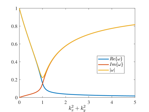
Figure 1: Illustration of the eigenvalue with complex $k_{z}$. Here, $k_{z}^{2}=1+0.1i$, $\alpha=1$ and $E=0$.

Complex $k_{z}$ is also physically reasonable. The top and bottom non-slip boundaries introduce an exponential decay form to the asymptotic solutions along the $z$-direction (Zhang & Liao (2009)), which agrees with our numerical results in Appendix A. Also, under open boundary conditions, i.e., with external energy injection, the bulk eigen states of non-Hermitian systems exhibit a localized behavior towards the border, the so-called non-Hermitian skin effect, which differs from the extended Bloch waves in Hermitian systems. In our system, energy exchanges with the outsiders in the $z$-direction due to the temperature difference, so we take a complex $k_{z}$.

3.2 Inviscid topological invariant ($E=0$)

With the generalized Brillouin zone where $k_{z}$ is complex, we can calculate the Chern number for open boundaries through a normal process, just as we do under periodic boundary conditions. The solutions satisfying realistic boundary conditions can be found in Appendix A. To obtain a single-valued function when dealing with the square root, we redefine the square root operation on the complex domain, making its value domain lie in the right half-plane that does not include the negative imaginary axis, i.e., $\sqrt{-1}=i$.

We start to discuss the topological properties of the system with the simplest case $E=0$. Since $k_{z}$ is complex, the singularity in the eigenvalues and eigenvectors will not exist. The Hamiltonian matrix becomes

$$H_{0}=i\left[\begin{array}[]{cccc}\lambda\frac{k_{x}k_{y}}{k^{2}}&\lambda(1-\frac{k_{x}^{2}}{k^{2}})&0&-\alpha\frac{k_{x}k_{z}}{k^{2}}\\ \lambda(-1+\frac{k_{y}^{2}}{k^{2}})&-\lambda\frac{k_{x}k_{y}}{k^{2}}&0&-\alpha\frac{k_{y}k_{z}}{k^{2}}\\ \lambda\frac{k_{y}k_{z}}{k^{2}}&-\lambda\frac{k_{x}k_{z}}{k^{2}}&0&\alpha-\alpha\frac{k_{z}^{2}}{k^{2}}\\ 0&0&1&0\end{array}\right].$$ (17)

For the eigen equation

$$H_{0}\psi=\omega\psi,$$ (18)

the non-zero eigenvalues and corresponding right eigenvectors are

$$\omega_{\pm}=\pm\omega_{0},\ \ \omega_{0}=\frac{\sqrt{k_{z}^{2}-\alpha(k_{x}^{2}+k_{y}^{2})}}{k},$$ (19)

$$\left.\left|\psi_{\pm}\right.\right\rangle=\frac{1}{\sqrt{2\left(\frac{k_{z}^{2}}{k_{x}^{2}+k_{y}^{2}}-\alpha\right)}}\left[\begin{array}[]{c}\frac{k_{z}\left(-i\lambda k_{y}\mp k_{x}\omega_{0}\right)}{k_{x}^{2}+k_{y}^{2}}\\ \frac{k_{z}\left(i\lambda k_{x}\mp k_{y}\omega_{0}\right)}{k_{x}^{2}+k_{y}^{2}}\\ \pm\omega_{0}\\ i\end{array}\right],$$ (20)

where $k=\sqrt{k_{x}^{2}+k_{y}^{2}+k_{z}^{2}}$ and $k_{x}^{2}+k_{y}^{2}\neq 0$. When $\rho=\sqrt{k_{x}^{2}+k_{y}^{2}}\xrightarrow{}0$, the eigenvectors become

$$\left.\left|\psi_{\pm}\right.\right\rangle=\frac{1}{\sqrt{2}}\left[\begin{array}[]{c}\pm\lambda i\\ 1\\ 0\\ 0\end{array}\right].$$ (21)

When $\rho\xrightarrow{}+\infty$, the eigenvectors are still single-valued that

$$\left.\left|\psi_{\pm}\right.\right\rangle=\frac{1}{\sqrt{2}}\left[\begin{array}[]{c}0\\ 0\\ \pm 1\\ \frac{i}{\sqrt{-\alpha}}\end{array}\right].$$ (22)

Thus, different from the shallow water model, the eigenvectors here are regular on a compact manifold, which guarantees a well-defined Chern number without introducing unphysical items (Tauber et al., 2019).

For the eigen equation

$$H_{0}^{\dagger}\psi^{\prime}=\omega^{\ast}\psi^{\prime},$$ (23)

the non-zero eigenvalues and corresponding left eigenvectors are

$$\omega_{\pm}^{\ast}=\pm\omega_{0}^{\ast},$$ (24)

$$\left\langle\left.\psi_{\pm}^{\prime}\right|\right.=\frac{1}{\sqrt{2\left(\frac{k_{z}^{2}}{k_{x}^{2}+k_{y}^{2}}-\alpha\right)}}\left[\begin{array}[]{c}\frac{k_{z}\left(i\lambda k_{y}\mp\frac{k_{x}}{\omega_{0}}\right)}{k_{x}^{2}+k_{y}^{2}}\\ \frac{k_{z}\left(-i\lambda k_{x}\mp\frac{k_{y}}{\omega_{0}}\right)}{k_{x}^{2}+k_{y}^{2}}\\ \mp\frac{\alpha}{\omega_{0}}\\ i\alpha\end{array}\right]^{\mathrm{T}},$$ (25)

when $k_{x}^{2}+k_{y}^{2}\neq 0$. When $\rho\xrightarrow{}0$, the eigenvectors become

$$\left\langle\left.\psi_{\pm}^{\prime}\right|\right.=\frac{1}{\sqrt{2}}\left[\begin{array}[]{c}\mp\lambda i\\ 1\\ 0\\ 0\end{array}\right]^{\mathrm{T}}.$$ (26)

When $\rho\xrightarrow{}+\infty$, the eigenvectors are single-valued that

$$\left\langle\left.\psi_{\pm}^{\prime}\right|\right.=\frac{1}{\sqrt{2}}\left[\begin{array}[]{c}0\\ 0\\ \pm 1\\ -i\sqrt{-\alpha}\end{array}\right]^{\mathrm{T}}.$$ (27)

Substituting the expressions of eigenvectors in Eq.(15), the Berry curvature of the positive band (associated with $\omega_{+}$ and $\omega_{+}^{\ast}$) becomes

$$\varOmega^{z}=-\lambda\frac{k_{z}^{2}\left[\rho^{2}k_{z}^{2}+2\alpha\left(\rho^{4}+4\rho^{2}k_{z}^{2}+2k_{z}^{4}\right)-\alpha^{2}\rho^{2}\left(2\rho^{2}+k_{z}^{2}\right)\right]}{2k^{3}\left(k_{z}^{2}-\alpha\rho^{2}\right)^{5/2}},$$ (28)

where $\rho=\sqrt{k_{x}^{2}+k_{y}^{2}}$. Then the Chern number is

$$C =\frac{1}{2\pi}\int_{-\infty}^{+\infty}\int_{-\infty}^{+\infty}\varOmega^{z}dk_{x}dk_{y}$$ (29a)

$$=\int_{0}^{+\infty}\rho\varOmega^{z}d\rho$$ (29b)

$$=\lambda\left.\frac{-2k_{z}^{4}+k_{z}^{2}(\alpha-1)\rho^{2}}{2\sqrt{\rho^{2}+k_{z}^{2}}\left(k_{z}^{2}-\alpha\rho^{2}\right)^{3/2}}\right|_{0}^{+\infty}$$ (29c)

$$=\lambda,$$ (29d)

which implies the existence of topologically protected edge states only related to the direction of fluid rotation. This is a three-dimensional version of the topologically protected equatorial waves (Delplace et al., 2017). Under the hydrostatic approximation, we obtain an exact two-dimensional counterpart, shown in Sec.5.

3.3 Topological invariant when $E\neq 0$

This section considers $E\neq 0$, which does not change the Chern number we obtained in the previous subsection. Firstly, When $Pr=1$, the Hamiltonian matrix $H$ becomes

$$H=H_{0}+iE_{0}\boldsymbol{\hat{1}},$$ (30)

where $H_{0}$ is the simple Hamiltonian where $E=0$ and $\boldsymbol{\hat{1}}$ is the unit matrix of the same order as $H_{0}$. The eigenvalues are

$$\omega_{\pm}=\pm\omega_{0}+iE_{0}.$$ (31)

It is just a shift of $\pm\omega_{0}$, the eigenvalues of $H_{0}$, and then the eigenvectors are independent of $E$. Therefore, both the Berry curvature and Chern number are unchanged compared with the case where $E=0$.

When $Pr\neq 1$, there are no simple expressions for the eigenvalues and eigenvectors, and we need to calculate the Chern number with the help of numerical calculations, seen in Figure 2. To avoid the derivation of the eigenvectors, we rewrite Eq.(15) as

$$\Omega_{n}^{z}=i\underset{m\neq n}{\sum}\frac{<\psi_{n}^{\prime}|\frac{\partial H}{\partial k_{x}}|\psi_{m}><\psi_{m}^{\prime}|\frac{\partial H}{\partial k_{y}}|\psi_{n}>-\{x\leftrightarrow y\}}{(\omega_{n}-\omega_{m})^{2}}.$$ (32)

It is similar to the Hermitian case (Xiao et al., 2010) except that the left vector takes the biorthogonal partner. This form is very useful for numerical calculations because it can be evaluated under an unsmooth phase choice of the eigenstates, which often occurs in the standard diagonalization algorithms.

Figure 2: Numerical results of the non-Hermitian Chern number. (a) Chern number with different Prandtl number $Pr$ and rotation directions $\lambda=\pm 1$. The upper limit of integral for $\rho$ is $k_{cut}=6$, the $k$-point accuracy per unit length is 200 (radial) * 200 (axial) using the Gauss-Legendre integration scheme. (b) Demonstrating the numerical convergence degree with different $k$-point accuracy as $k_{cut}$ increases. Other parameters are $\alpha=1$, $E=0.01$, $k_{z}=1+0.1i$.

4 The stably stratified and critical cases

Even though this paper focuses on the unstably stratified convection situation, this section shows that following the above-mentioned procedure for calculating the Chern number in non-Hermitian systems we can recover the classic results in the stably stratified situations (e.g. Delplace et al., 2017). For the simple case that $E=0$, when $\alpha<0$, the eigenvalues of the linearized equations Eqs. (2)-(4) are real, and the system is stable without oscillatory modes that can grow or decay over time. At this time the discussion in the previous section where $\alpha>0$ still holds, and the system still has a non-zero Chern number $C=\lambda$. Thus, the existence of the tenacious wall modes in the stratified fluid relies only on rotation, regardless of the driving mechanism.

When $\alpha=0$, the system is in a critical neutral state, and the eigenvalues of the Hamiltonian are

$$\omega_{1}\equiv\omega_{+} =\frac{k_{z}}{k}-iEk^{2},$$ (33a)

$$\omega_{2}\equiv\omega_{-} =-\frac{k_{z}}{k}-iEk^{2},$$ (33b)

$$\omega_{3} =-i\frac{E}{Pr}k^{2},$$ (33c)

$$\quad\omega_{4} =-iEk^{2}.$$ (33d)

Considering the symmetry between $\omega_{+}$ and $\omega_{-}$, we have assumed that $Re\{k_{z}\}>0$. The Berry curvature of band $\omega_{3}$ (or $\omega_{4}$) is 0. The Berry curvature of band $\omega_{\pm}$ reads

$$\varOmega^{z}_{\pm}=\mp\lambda\frac{k_{x}^{2}+k_{y}^{2}}{2k_{z}k^{3}},$$ (34)

which is independent of $E$ and $Pr$. The integral does not converge when we evaluate the Chern number

$$C_{\pm}=\frac{1}{2\pi}\int_{-\infty}^{+\infty}\int_{-\infty}^{+\infty}\varOmega^{z}_{\pm}dk_{x}dk_{y}=\int_{0}^{+\infty}\frac{\mp\lambda\rho^{3}}{2k_{z}(\rho^{2}+k_{z}^{2})^{3/2}}d\rho.$$ (35)

Mathematically, this is due to the degeneration of $\omega_{+}$ and $\omega_{-}$ at $\rho\xrightarrow{}+\infty$, which leads to the close of the band gap of the system. The critical case is important to show that stratification is crucial, whether stable or unstable.

5 Hydrostatic approximation

Under the hydrostatic approximation, the $z$-direction momentum equation of (2) reduces to

$$\hat{\theta}=\frac{i\hat{p}k_{z}}{\alpha}.$$ (36)

From Eq.(3) we get

$$\hat{w}=-\frac{k_{x}\hat{u}+k_{y}\hat{v}}{k_{z}}.$$ (37)

With the wave vector $\psi\equiv(\hat{u},\hat{v},\hat{p})$, we get the eigen equations from Eq.(2) and Eq.(4) as

$$H=\left[\begin{array}[]{ccc}iE_{0}&i\lambda&k_{x}\\ -i\lambda&iE_{0}&k_{y}\\ -\alpha\frac{k_{x}}{k_{z}^{2}}&-\alpha\frac{k_{y}}{k_{z}^{2}}&iE_{1}\end{array}\right],$$ (38)

where $E_{0}=-Ek^{2}$, $E_{1}=E_{0}/Pr$. This is a non-Hermitian Hamiltonian because $H\neq H^{\dagger}$, but for the stable case where $\alpha<0$, it can be changed into a Hermitian one by replacing the variables. If we further assume that $Pr=1$, the Hamiltonian is an analogue of the one in topological shallow water waves in Delplace et al. (2017), except for a frequency shift. However, for the unstable case with $\alpha>0$, the non-Hermitian nature of the system is intrinsic and cannot be turned into a Hermitian one by variable substitutions.

For the eigen equation

$$H\psi=\omega\psi,$$ (39)

the eigenvalues and eigenvectors contributing to non-zero Chen numbers are ($Pr=1$)

$$\omega_{\pm}=\pm\omega_{0}-iEk^{2},\ \ \omega_{0}=\sqrt{1-\frac{\alpha}{k_{z}^{2}}(k_{x}^{2}+k_{y}^{2})},$$ (40)

$$\left.\left|\psi_{\pm}\right.\right\rangle=\frac{1}{\sqrt{2\left(\frac{k_{z}^{2}}{k_{x}^{2}+k_{y}^{2}}-\alpha\right)}}\left[\begin{array}[]{c}\frac{k_{z}^{2}\left(i\lambda k_{y}\pm k_{x}\omega_{0}\right)}{k_{x}^{2}+k_{y}^{2}}\\ \frac{k_{z}^{2}\left(-i\lambda k_{x}\pm k_{y}\omega_{0}\right)}{k_{x}^{2}+k_{y}^{2}}\\ -\alpha\end{array}\right].$$ (41)

When $\rho\xrightarrow{}0$, the eigenvectors become

$$\left.\left|\psi_{\pm}\right.\right\rangle=\frac{1}{\sqrt{2}}\left[\begin{array}[]{c}\pm\lambda i\\ 1\\ 0\end{array}\right].$$ (42)

When $\rho\xrightarrow{}+\infty$, the eigenvectors become

$$\left.\left|\psi_{\pm}\right.\right\rangle=\frac{1}{\sqrt{2}}\left[\begin{array}[]{c}\pm\sqrt{k_{z}^{2}}\frac{k_{x}}{\rho}\\ \pm\sqrt{k_{z}^{2}}\frac{k_{y}}{\rho}\\ \sqrt{-\alpha}\end{array}\right],$$ (43)

which are not single-valued in different directions. In order to get a compact manifold where the Chern number is well defined, we may need to introduce an odd viscosity term like in the shallow water model (Tauber et al., 2019).

For the eigen equation

$$H^{\dagger}\psi^{\prime}=\omega^{\prime}\psi^{\prime},$$ (44)

we have

$$\omega_{\pm}^{\prime}=\omega_{\pm}^{\ast},$$ (45)

$$\left\langle\left.\psi_{\pm}^{\prime}\right|\right.=\frac{1}{\sqrt{2\left(\frac{k_{z}^{2}}{k_{x}^{2}+k_{y}^{2}}-\alpha\right)}}\left[\begin{array}[]{c}\frac{-i\lambda k_{y}\pm k_{x}\omega_{0}}{k_{x}^{2}+k_{y}^{2}}\\ \frac{i\lambda k_{x}\pm k_{y}\omega_{0}}{k_{x}^{2}+k_{y}^{2}}\\ 1\end{array}\right]^{\mathrm{T}}.$$ (46)

When $\rho\xrightarrow{}0$, the eigenvectors become

$$\left\langle\left.\psi_{\pm}^{\prime}\right|\right.=\frac{1}{\sqrt{2}}\left[\begin{array}[]{c}\mp\lambda i\\ 1\\ 0\end{array}\right]^{\mathrm{T}}.$$ (47)

When $\rho\xrightarrow{}+\infty$, the eigenvectors become

$$\left\langle\left.\psi_{\pm}^{\prime}\right|\right.=\frac{1}{\sqrt{2}}\left[\begin{array}[]{c}\pm\frac{k_{x}}{\rho\sqrt{k_{z}^{2}}}\\ \pm\frac{k_{y}}{\rho\sqrt{k_{z}^{2}}}\\ \frac{1}{\sqrt{-\alpha}}\end{array}\right].$$ (48)

The Berry curvature of the positive band (associated with $\omega_{+}$ and $\omega_{+}^{\prime}$) is

$$\varOmega^{z}=-\frac{\lambda\alpha\sqrt{k_{z}^{2}}}{\left(k_{z}^{2}-\alpha\rho^{2}\right)^{3/2}},$$ (49)

where $\rho=\sqrt{k_{x}^{2}+k_{y}^{2}}$. Then the Chern number is

$$C =\frac{1}{2\pi}\int_{-\infty}^{+\infty}\int_{-\infty}^{+\infty}\varOmega^{z}dk_{x}dk_{y}$$ (50a)

$$=\int_{0}^{+\infty}\rho\varOmega^{z}d\rho$$ (50b)

$$=\left.-\frac{\lambda\sqrt{k_{z}^{2}}}{\sqrt{k_{z}^{2}-\alpha\rho^{2}}}\right|_{0}^{+\infty}$$ (50c)

$$=\lambda.$$ (50d)

In the stably stratified case, $\alpha<0$, the above calculation holds when $Re\{k_{z}\}\neq 0$; while in the unstably stratified case, $\alpha>0$, we need $Im\{k_{z}\}\neq 0$. If the system is neutral, $\alpha=0$, we arrive at two gapped flat bands $\omega_{\pm}=\pm 1-iEk^{2}$, which differ from the degenerate scenario in Eq.(33), and obtain $C=0$ since $\varOmega^{z}=0$.

6 Winding number

To put the topological nature of the system into perspective, we define a complex function in the wavenumber space $(k_{x},k_{y})$ (cf. Zhu et al., 2023):

$$\Xi(\boldsymbol{k})=\hat{v}(\boldsymbol{k})\hat{w}^{\ast}(\boldsymbol{k}),$$ (51)

which removes the gauge redundancy of the eigenfunctions, leaving only the internal phase difference between the two components. Figure 3 depicts the argument of $\Xi(\boldsymbol{k})$, $\tan^{-1}(Re\{\Xi\}/Im\{\Xi\})$, whose x and y components represent the real and imaginary parts of $\Xi$ with a rescaled equal length. When $\lambda=1$, there is a vortex formed by the vector arrows going in the anticlockwise direction, and the arrows along a closed circle smoothly wind by a phase of 2$\pi$, suggesting a winding number of $1$. Conversely, when $\lambda=-1$, there is a strain flow with the winding number of $-1$.

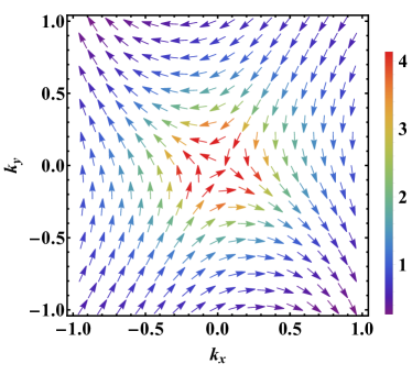
Figure 3: Arrows representing argument of $\Xi(\boldsymbol{k})=\hat{v}(\boldsymbol{k})*\hat{w}^{\ast}(\boldsymbol{k})$ with $\lambda=1$ (left) and $\lambda=-1$ (right). The x and y components of the arrow represent the real and imaginary parts of $\Xi(\boldsymbol{k})$. The length of the arrows is rescaled to be equal. Colors represent normalized magnitude $|\Xi(\boldsymbol{k})|$ in arbitrary units. Other parameters are $Pr=1$, $\alpha=0.5$, $k_{z}=1+0.5i$.

7 Summary and Discussion

In summary, we show that the linearized rotating Rayleigh-Bénard convection can support non-Hermitian topological states characterized by a non-zero integer Chern number. Thus, we verify the hypothesis by Favier & Knobloch (2020) that the robust wall modes in rapidly rotating convection are topologically protected. Due to the unstable stratification, the linear eigenvalue problem is intrinsically non-Hermitian, so the Berry curvature is defined on biorthogonal eigenstates, and the corresponding eigenvalues may be complex, which is very different from the Hermitian system. Beyond the shallow water model, the eigenvectors here are regular on a compact manifold, which guarantees a well-defined Chern number without introducing unphysical items (Tauber et al., 2019). The emergence of these topological edge states is fundamentally due to rotation breaking the system’s time-reversal symmetry, but stratification also plays a crucial role: without the stratification, i.e., for the critical case, the bulk Chern number is either not well-defined or equals zero. Under the hydrostatic approximation, the problem transforms into a two-dimensional counterpart of the one that explains the topological origin of equatorial waves (Delplace et al., 2017). Finally, an eigenvector-dependent winding number is introduced to visualize the topological nature of the fluid.

On the precession direction of the edge states, they are usually (not all) retrograde in rotating convection (Zhong et al., 1991; Goldstein et al., 1993; Kuo & Cross, 1993; Herrmann & Busse, 1993), but prograde both at the Earth’s equator and in the two-dimensional fluids with odd viscosity (Delplace et al., 2017; Souslov et al., 2019). This is a result of the combined contribution of the boundary conditions and the system parameters, especially the effect of the Prandtl number $Pr$ (Goldstein et al., 1994; Horn & Schmid, 2017). It is quite different from the conventional Hermitian system with periodic boundary conditions, where the positive or negative sign of the Chen number determines the direction of the edge states (Hasan & Kane, 2010; Essin & Gurarie, 2011).

For simplicity, we assume both $k_{x}$ and $k_{y}$ to be real numbers. Thus, according to the regular formalities (Souslov et al., 2019), the non-zero Chern number we obtain describes the topological properties of the system without boundary in the $x-y$ plane. When there is an impenetrable and slippery wall, the bulk-boundary correspondence ensures the existence of topologically protected edge states (Essin & Gurarie, 2011). When the wall is non-slip, we can still get a well-defined non-zero Chern number, but in this case, $k_{x}$ and $k_{y}$ need to be taken as complex numbers (Yao et al., 2018).

The Rayleigh-Bénard convection is essentially a nonlinear system, so as a complement to the conclusions of this paper, it is necessary to continue to investigate the nonlinear effects on the topological properties of the bulk states. We expect that weak nonlinear effects do not destroy the topological invariance of the system, partly because the topological properties are robust to perturbations and partly because previous numerical simulations imply this (Favier & Knobloch, 2020). For a more detailed quantitative analysis, we need to evaluate the generalized geometric phase in the case of non-eigen states (Liu et al., 2003; Wu et al., 2005).

Acknowledgement This work has received financial support from the National Natural Science Foundation of China (NSFC) under grant NO. 92052102 and 12272006, and from the Laoshan Laboratory under grant NO. 2022QNLM010201.

Appendix A Solutions satisfying realistic boundary conditions

Unlike in Hermitian systems, the eigen frequencies and solutions of non-Hermitian systems are very sensitive to the boundary conditions. For simplicity, we assume that the horizontal direction is unbounded and the $z$-direction takes the no-slip boundary condition that

$$u=v=w=\theta=0\text{\quad on \quad}z=0,1.$$ (52)

To ensure that our analyses above match a realistic situation, we construct solutions in the form that

$$\phi=e^{i(k_{x}x+k_{y}y-\omega t)}\sum_{i=1}^{4}\lambda_{i}e^{ik_{zi}z}\left.\left|\psi_{i}\right.\right\rangle,$$ (53)

where $\left.\left|\psi_{i}\right.\right\rangle$ is the eigenvector of Hamiltonian (30) corresponding to $k_{zi}$. According to our calculations above, when the system evolves along a closed path in its parameter space, $\left.\left|\psi_{1-4}\right.\right\rangle$ will all get the Berry phase of $2\pi\lambda$. As a result, the solution $\phi$ also gets the same Berry phase. For a particular frequency $\omega(k_{x},k_{y})$, $k_{z1-4}$ come from the dispersion relation that ($Pr=1$)

$$\omega=\frac{\sqrt{k_{z}^{2}-\alpha(k_{x}^{2}+k_{y}^{2})}}{k}-iEk^{2}.$$ (54)

Generally, the solved $k_{zi}$ is complex, and $k_{z3}=-k_{z1}$, $k_{z4}=-k_{z2}$.

For the no-slip boundary condition, we have

$$M\left[\begin{array}[]{c}\lambda_{1}\\ \lambda_{2}\\ \lambda_{3}\\ \lambda_{4}\end{array}\right]=0,$$ (55)

where

$$M=\left[\begin{array}[]{cccc}1&1&1&1\\ k_{z1}&k_{z2}&k_{z3}&k_{z4}\\ e^{ik_{z1}}&e^{ik_{z2}}&e^{ik_{z3}}&e^{ik_{z4}}\\ e^{ik_{z1}}k_{z1}&e^{ik_{z2}}k_{z2}&e^{ik_{z3}}k_{z3}&e^{ik_{z4}}k_{z4}\end{array}\right].$$ (56)

To get a nontrivial solution of $\lambda_{i}(k_{x},k_{y})$, we have

$$det(M)=0,$$ (57)

and obtain that

$$2k_{z1}k_{z2}(-1+\cos{k_{z1}}\cos{k_{z2}})+(k_{z1}^{2}+k_{z2}^{2})\sin{k_{z1}}\sin{k_{z2}}=0.$$ (58)

Obviously, $k_{z1}=k_{z2}$ satisfies the above equation, but this will give a trivial solution that $\lambda_{i}(k_{x},k_{y})=0$ and we do not choose it. Combining with Eq.(54), one can identify the nontrivial values of $k_{zi}$, $\omega(k_{x},k_{y})$ and $\lambda_{i}(k_{x},k_{y})$. As an example, for parameters $k_{x}=k_{y}=0.5$, $\alpha=1$ and $E=0.01$, numerical calculation gives that $\omega\approx 0.9903-0.8108i$, $k_{z1}\approx 8.9763-0.0195i$, $k_{z2}\approx 0.3998-0.6643i$ and

$$\left[\begin{array}[]{c}\lambda_{1}\\ \lambda_{2}\\ \lambda_{3}\\ \lambda_{4}\end{array}\right]=\mathcal{C}\left[\begin{array}[]{c}1\\ 0.9877-1.5056i\\ 0.9188-0.4422i\\ -2.9066+1.9478i\end{array}\right],$$ (59)

where $\mathcal{C}$ is an arbitrary constant.

References

- Ahlers et al. (2009) Ahlers, Guenter, Grossmann, Siegfried & Lohse, Detlef 2009 Heat transfer and large scale dynamics in turbulent rayleigh-bénard convection. Rev. Mod. Phys. 81, 503–537.
- Ashida et al. (2020) Ashida, Yuto, Gong, Zongping & Ueda, Masahito 2020 Non-hermitian physics. Advances in Physics 69 (3), 249–435.
- Bergholtz et al. (2021) Bergholtz, Emil J., Budich, Jan Carl & Kunst, Flore K. 2021 Exceptional topology of non-hermitian systems. Rev. Mod. Phys. 93, 015005.
- Berry (1984) Berry, Michael Victor 1984 Quantal phase factors accompanying adiabatic changes. Proceedings of the Royal Society of London. A. Mathematical and Physical Sciences 392 (1802), 45–57.
- Bodenschatz et al. (2000) Bodenschatz, Eberhard, Pesch, Werner & Ahlers, Guenter 2000 Recent developments in rayleigh-bénard convection. Annual Review of Fluid Mechanics 32 (1), 709–778.
- Chandrasekhar (1961) Chandrasekhar, S 1961 Hydrodynamic and hydromagnetic stability .
- Delplace et al. (2017) Delplace, Pierre, Marston, J. B. & Venaille, Antoine 2017 Topological origin of equatorial waves. Science 358 (6366), 1075–1077.
- Ding et al. (2022) Ding, Kun, Fang, Chen & Ma, Guancong 2022 Non-hermitian topology and exceptional-point geometries. Nature Reviews Physics pp. 1–16.
- Ecke (2023) Ecke, Robert E. 2023 Rotating rayleigh–bénard convection: Bits and pieces. Physica D: Nonlinear Phenomena 444, 133579.
- Ecke & Shishkina (2023) Ecke, Robert E. & Shishkina, Olga 2023 Turbulent rotating rayleigh–bénard convection. Annual Review of Fluid Mechanics 55 (1), 603–638.
- Ecke et al. (2022) Ecke, Robert E., Zhang, Xuan & Shishkina, Olga 2022 Connecting wall modes and boundary zonal flows in rotating rayleigh-bénard convection. Phys. Rev. Fluids 7, L011501.
- Ecke et al. (1992) Ecke, R. E., Zhong, Fang & Knobloch, E. 1992 Hopf bifurcation with broken reflection symmetry in rotating rayleigh-bénard convection. Europhysics Letters 19 (3), 177.
- Essin & Gurarie (2011) Essin, Andrew M. & Gurarie, Victor 2011 Bulk-boundary correspondence of topological insulators from their respective green’s functions. Phys. Rev. B 84, 125132.
- Favier & Knobloch (2020) Favier, Benjamin & Knobloch, Edgar 2020 Robust wall states in rapidly rotating rayleigh-bénard convection. Journal of Fluid Mechanics 895, R1.
- Goldstein et al. (1993) Goldstein, H. F., Knobloch, E., Mercader, I. & Net, M. 1993 Convection in a rotating cylinder. part 1 linear theory for moderate prandtl numbers. Journal of Fluid Mechanics 248, 583–604.
- Goldstein et al. (1994) Goldstein, H. F., Knobloch, E., Mercader, I. & Net, M. 1994 Convection in a rotating cylinder. part 2. linear theory for low prandtl numbers. Journal of Fluid Mechanics 262, 293–324.
- Guervilly et al. (2014) Guervilly, Céline, Hughes, David W. & Jones, Chris A. 2014 Large-scale vortices in rapidly rotating rayleigh-bénard convection. Journal of Fluid Mechanics 758, 407–435.
- Haldane (1988) Haldane, F. D. M. 1988 Model for a quantum hall effect without landau levels: Condensed-matter realization of the ”parity anomaly”. Phys. Rev. Lett. 61, 2015–2018.
- Hasan & Kane (2010) Hasan, M. Z. & Kane, C. L. 2010 Colloquium: Topological insulators. Rev. Mod. Phys. 82, 3045–3067.
- Herrmann & Busse (1993) Herrmann, J. & Busse, F. H. 1993 Asymptotic theory of wall-attached convection in a rotating fluid layer. Journal of Fluid Mechanics 255, 183–194.
- Horn & Schmid (2017) Horn, Susanne & Schmid, Peter J. 2017 Prograde, retrograde, and oscillatory modes in rotating rayleigh–bénard convection. Journal of Fluid Mechanics 831, 182–211.
- King et al. (2012) King, E. M., Stellmach, S. & Aurnou, J. M. 2012 Heat transfer by rapidly rotating rayleigh-bénard convection. Journal of Fluid Mechanics 691, 568–582.
- Kosterlitz & Thouless (1973) Kosterlitz, John Michael & Thouless, David James 1973 Ordering, metastability and phase transitions in two-dimensional systems. Journal of Physics C: Solid State Physics 6 (7), 1181.
- Kuo & Cross (1993) Kuo, E. Y. & Cross, M. C. 1993 Traveling-wave wall states in rotating rayleigh-bénard convection. Phys. Rev. E 47, R2245–R2248.
- Liu et al. (2003) Liu, Jie, Wu, Biao & Niu, Qian 2003 Nonlinear evolution of quantum states in the adiabatic regime. Phys. Rev. Lett. 90, 170404.
- Liu et al. (2020) Liu, Yizhou, Chen, Xiaobin & Xu, Yong 2020 Topological phononics: From fundamental models to real materials. Advanced Functional Materials 30 (8), 1904784, arXiv: https://onlinelibrary.wiley.com/doi/pdf/10.1002/adfm.201904784.
- Liu & Ecke (1999) Liu, Yuanming & Ecke, Robert E. 1999 Nonlinear traveling waves in rotating rayleigh-bénard convection: Stability boundaries and phase diffusion. Phys. Rev. E 59, 4091–4105.
- Ning & Ecke (1993) Ning, Li & Ecke, Robert E. 1993 Rotating rayleigh-bénard convection: Aspect-ratio dependence of the initial bifurcations. Phys. Rev. E 47, 3326–3333.
- Ozawa et al. (2019) Ozawa, Tomoki, Price, Hannah M., Amo, Alberto, Goldman, Nathan, Hafezi, Mohammad, Lu, Ling, Rechtsman, Mikael C., Schuster, David, Simon, Jonathan, Zilberberg, Oded & Carusotto, Iacopo 2019 Topological photonics. Rev. Mod. Phys. 91, 015006.
- Perez et al. (2021) Perez, N., Delplace, P. & Venaille, A. 2021 Manifestation of the berry curvature in geophysical ray tracing. Proceedings of the Royal Society A: Mathematical, Physical and Engineering Sciences 477 (2248), 20200844.
- Rossby (1969) Rossby, H. T. 1969 A study of bénard convection with and without rotation. Journal of Fluid Mechanics 36 (2), 309–335.
- Senthil (2015) Senthil, Todadri 2015 Symmetry-protected topological phases of quantum matter. Annu. Rev. Condens. Matter Phys. 6 (1), 299–324.
- Shankar et al. (2022) Shankar, Suraj, Souslov, Anton, Bowick, Mark J, Marchetti, M Cristina & Vitelli, Vincenzo 2022 Topological active matter. Nature Reviews Physics 4 (6), 380–398.
- Shen et al. (2018) Shen, Huitao, Zhen, Bo & Fu, Liang 2018 Topological band theory for non-hermitian hamiltonians. Phys. Rev. Lett. 120, 146402.
- Souslov et al. (2019) Souslov, Anton, Dasbiswas, Kinjal, Fruchart, Michel, Vaikuntanathan, Suriyanarayanan & Vitelli, Vincenzo 2019 Topological waves in fluids with odd viscosity. Phys. Rev. Lett. 122, 128001.
- Tauber et al. (2019) Tauber, C., Delplace, P. & Venaille, A. 2019 A bulk-interface correspondence for equatorial waves. Journal of Fluid Mechanics 868, R2.
- Terrien et al. (2023) Terrien, Louise, Favier, Benjamin & Knobloch, Edgar 2023 Suppression of wall modes in rapidly rotating rayleigh-bénard convection by narrow horizontal fins. Phys. Rev. Lett. 130, 174002.
- Thouless et al. (1982) Thouless, David J, Kohmoto, Mahito, Nightingale, M Peter & den Nijs, Marcel 1982 Quantized hall conductance in a two-dimensional periodic potential. Physical review letters 49 (6), 405.
- Venaille & Delplace (2021) Venaille, A. & Delplace, P. 2021 Wave topology brought to the coast. Phys. Rev. Res. 3, 043002.
- Venaille et al. (2023) Venaille, Antoine, Onuki, Yohei, Perez, Nicolas & Leclerc, Armand 2023 From ray tracing to waves of topological origin in continuous media. SciPost Phys. 14, 062.
- de Wit et al. (2020) de Wit, Xander M., Aguirre Guzmán, Andrés J., Madonia, Matteo, Cheng, Jonathan S., Clercx, Herman J. H. & Kunnen, Rudie P. J. 2020 Turbulent rotating convection confined in a slender cylinder: The sidewall circulation. Phys. Rev. Fluids 5, 023502.
- Wu et al. (2005) Wu, Biao, Liu, Jie & Niu, Qian 2005 Geometric phase for adiabatic evolutions of general quantum states. Phys. Rev. Lett. 94, 140402.
- Xiao et al. (2010) Xiao, Di, Chang, Ming-Che & Niu, Qian 2010 Berry phase effects on electronic properties. Reviews of modern physics 82 (3), 1959.
- Yao et al. (2018) Yao, Shunyu, Song, Fei & Wang, Zhong 2018 Non-hermitian chern bands. Phys. Rev. Lett. 121, 136802.
- Zak (1989) Zak, J 1989 Berry’s phase for energy bands in solids. Physical review letters 62 (23), 2747.
- Zhang & Liao (2009) Zhang, Keke & Liao, Xinhao 2009 The onset of convection in rotating circular cylinders with experimental boundary conditions. Journal of Fluid Mechanics 622, 63–73.
- Zhang et al. (2020) Zhang, Xuan, van Gils, Dennis P. M., Horn, Susanne, Wedi, Marcel, Zwirner, Lukas, Ahlers, Guenter, Ecke, Robert E., Weiss, Stephan, Bodenschatz, Eberhard & Shishkina, Olga 2020 Boundary zonal flow in rotating turbulent rayleigh-bénard convection. Phys. Rev. Lett. 124, 084505.
- Zhong et al. (1991) Zhong, Fang, Ecke, Robert & Steinberg, Victor 1991 Asymmetric modes and the transition to vortex structures in rotating rayleigh-bénard convection. Phys. Rev. Lett. 67, 2473–2476.
- Zhong et al. (1993) Zhong, Fang, Ecke, Robert E. & Steinberg, Victor 1993 Rotating rayleigh–bénard convection: asymmetric modes and vortex states. Journal of Fluid Mechanics 249, 135–159.
- Zhong et al. (2009) Zhong, Jin-Qiang, Stevens, Richard J. A. M., Clercx, Herman J. H., Verzicco, Roberto, Lohse, Detlef & Ahlers, Guenter 2009 Prandtl-, rayleigh-, and rossby-number dependence of heat transport in turbulent rotating rayleigh-bénard convection. Phys. Rev. Lett. 102, 044502.
- Zhu et al. (2023) Zhu, Ziyan, Li, Christopher & Marston, J. B. 2023 Topology of rotating stratified fluids with and without background shear flow. Phys. Rev. Res. 5, 033191.