Elucidating the impact of massive neutrinos on halo assembly bias

Abstract

Massive neutrinos have non-negligible impact on the formation of large-scale structures. We investigate the impact of massive neutrinos on the halo assembly bias effect, measured by the relative halo bias $\hat{b}$ as a function of the curvature of the initial density peak $\hat{s}$, neutrino excess $\epsilon_{\nu}$, or halo concentration $\hat{c}$, using a large suite of $\Sigma M_{\nu}{=}0.0$ eV and $0.4$ eV simulations with the same initial conditions. By tracing dark matter haloes back to their initial density peaks, we construct a catalogue of halo “twins” that collapsed from the same peaks but evolved separately with and without massive neutrinos, thereby isolating any effect of neutrinos on halo formation. We detect a $2\%$ weakening of the halo assembly bias as measured by $\hat{b}(\epsilon_{\nu})$ in the presence of massive neutrinos. Due to the significant correlation between $\hat{s}$ and $\epsilon_{\nu}$ ($r_{cc}{=}0.319$), the impact of neutrinos persists in the halo assembly bias measured by $\hat{b}(\hat{s})$ but reduced by an order of magnitude to $0.1\%$. As the correlation between $\hat{c}$ and $\epsilon_{\nu}$ drops to $r_{cc}{=}0.087$, we do not detect any neutrino-induced impact on $\hat{b}(\hat{c})$, consistent with earlier studies. We also discover an equivalent assembly bias effect for the “neutrino haloes”, whose concentrations are anti-correlated with the large-scale clustering of neutrinos.

1 Introduction

Massive neutrinos play a key role in the formation of large-scale structures (LSS) of the Universe (Lesgourgues & Pastor, 2006; Wong, 2011). Their lack of clustering on scales below the free-streaming length induces a scale-dependent growth of the LSS, which enables stringent constraints of the sum of neutrino masses $\Sigma{M_{\nu}}$ with cosmological probes (Cuesta et al., 2016; Vagnozzi et al., 2017; Brinckmann et al., 2019; Dvorkin et al., 2019; Giusarma et al., 2016; Planck Collaboration et al., 2020; Alam et al., 2017; Ivanov et al., 2020; Palanque-Delabrouille et al., 2020; Di Valentino et al., 2021). Another important effect caused by the massive neutrinos is the differential growth of dark matter haloes between environments of different neutrino-to-dark matter density ratios (Yu et al., 2017). Through this effect, the presence of massive neutrinos may cause an impact on the so-called “halo assembly bias” (hereafter referred to as HAB; Gao & White, 2007), potentially opening a new avenue for measuring $\Sigma{M_{\nu}}$ with LSS observations. However, such impact can only be weak at best, as it has so far evaded detections in the simulations (Lazeyras et al., 2021). In this letter, we focus on the “twin” haloes collapsed from the same initial density peaks but evolved separately with and without massive neutrinos, aiming to elucidate the impact of massive neutrinos on the assembly bias of massive haloes.

HAB has been robustly predicted by the hierarchical structure formation of $\Lambda$+cold dark matter (CDM) simulations (Sheth & Tormen, 2004; Gao et al., 2005; Wechsler et al., 2006; Harker et al., 2006; Jing et al., 2007; Li et al., 2008). It has increasingly been referred to as the “secondary bias” (Salcedo et al., 2018; Mao et al., 2018) — the large-scale bias of haloes depends not only on halo mass, but also on other halo properties such as concentration, formation time, and spin. At any given halo mass $M_{h}$, the strength of HAB is often characterised by the relative halo bias $\hat{b}$ as a function of some “indicator” property $x$,

$$\hat{b}(x|M_{h})={b(x|M_{h})}\,/\,{\langle b|M_{h}\rangle},$$ (1)

where $b(x|M_{h})$ is the bias of haloes with $x$ and $\langle b|M_{h}\rangle$ is the overall bias at $M_{h}$. Contreras et al. (2021) found that HAB is independent of cosmological parameters in the $\Lambda$CDM, at least for the high-mass haloes that we focus on in this letter. Such an independence on cosmology could be useful for measuring $\Sigma{M_{\nu}}$, if HAB turns out to be sensitive to massive neutrinos.

Observationally, HAB at the high mass end has been at the brink of detection recently (Yang et al., 2006; Lin et al., 2016; Miyatake et al., 2016; Zu et al., 2017; Lin et al., 2022; Zu et al., 2021; Sunayama et al., 2022; Zu et al., 2022). Using cluster weak lensing, Zu et al. (2021) found that the stellar mass of the central galaxies is a good observational proxy for concentration. Combining with the $\hat{b}$ measurements from cluster-galaxy cross-correlations, Zu et al. (2022) detected a possible evidence of the cluster assembly bias, thereby demonstrating a viable path to accurate HAB measurements using future cluster surveys. In particular, $\Lambda$CDM simulations predict that the cluster-mass haloes with higher concentrations have a lower bias than their low-concentration counterparts. Dalal et al. (2008, hereafter referred to as D08) explained this phenomenon using the peak formalism (Kaiser, 1984; Bardeen et al., 1986; Sheth & Tormen, 1999), which predicts that the curvature of initial density peaks is correlated with the large-scale overdensity at fixed peak height. Using simulations, D08 demonstrated that the rare peaks with steep curvatures are more likely to collapse into clusters with high concentrations in low-density environments, and vice versa for those with shallow curvatures. In this letter, we follow D08 to trace haloes back to their initial density peaks and employ their peak curvature as a key indicator of HAB.

Although the presence of massive neutrinos delays the collapse of initial density peaks into haloes, the collapse time remains accurately predicted by the excursion set theory (Press & Schechter, 1974; Bond et al., 1991) if the variance of the CDM (assuming baryons follow the CDM) rather than the total mass field is considered (Ichiki & Takada, 2012). Therefore, it is perhaps unsurprising that Lazeyras et al. (2021) did not find any impact of neutrinos on HAB. However, Yu et al. (2017) discovered that the mass of haloes in neutrino-rich environments tends to be systematically higher than those in neutrino-poor regions, probably due to the higher capturing rate of the slow-moving neutrinos in neutrino-rich environments. If halo assembly histories are coherently modulated by neutrinos across different environments, it is reasonable to expect such a modulation to leave some discernible imprint on the HAB in simulations. To isolate the impact of neutrinos, we construct a catalogue of “twin” haloes that originated from the same initial density peaks but evolved separately in massless vs. massive neutrino cosmologies. Therefore, any difference of HAB between the two twin samples would provide a smoking gun evidence of the impact of neutrinos on HAB.

This letter is organized as follows. We describe the construction of our peak-based twin halo catalogue in Section 2 and present the HAB comparison using different indicators in Section 3. We summarize our results and look to the future in Section 4. Throughout this letter, we adopt a spherical overdensity-based halo definition so that the inner overdensity within halo radius $r_{200m}$ is 200 times the mean density of the Universe, and the halo mass $M_{h}$ is defined as the total mass enclosed by $r_{200m}$.

2 Peak-based Twin Halo Catalogue

We compare the HAB effects with and without massive neutrinos using the Quijote simulations (Villaescusa-Navarro et al., 2020), the same suite used by Lazeyras et al. (2021). Among the vast Quijote ensemble, we select one “Fiducial” set of 40 $\Lambda$CDM simulations with $\Sigma{M_{\nu}}{=}0.0\,\mathrm{ev}$, and another “$M_{\nu}^{+++}$” set of 40 massive neutrino simulations with $\Sigma{M_{\nu}}{=}0.4\,\mathrm{ev}$, hereafter referred to as the ${\nu}0.0$ and ${\nu}0.4$ simulations, respectively. The ${\nu}0.4$ simulations bear the highest $\Sigma{M_{\nu}}$ within the Quijote suite, so that any possible neutrino-induced HAB would exhibit the strongest signal. Both the CDM and neutrinos are particle-based, with $512^{3}$ CDM particles in a comoving volume of $1\,h^{-3}\mathrm{Gpc}^{3}$ of each simulation and an additional $512^{3}$ neutrino particles for each ${\nu}0.4$ run. The two sets of simulations have the same cosmological parameters, with $\Omega_{m}{=}0.3175$, $\Omega_{b}{=}0.049$, $h{=}0.6711$, $n_{s}{=}0.9624$, $\sigma_{8}=0.834$, and $\omega{=}{-}1$. More important, identical CDM initial conditions (with the same phases) at $z{=}127$ are shared by each of the 40 pair of ${\nu}0.0$ and ${\nu}0.4$ simulations, so that the haloes found at $z{=}0$ can always be mapped back to the initial density peaks in the $z{=}127$ snapshots. We identify dark matter haloes in the $z{=}0$ outputs of the 40 pairs of simulations using ROCKSTAR (Behroozi et al., 2013). We calculate halo concentration $c$ using the maximum circular velocity method (Prada et al., 2012), and use the relative concentration $\hat{c}$, defined as

$$\hat{c}\equiv\frac{c-\langle c|M_{h}\rangle}{\sigma_{c}(M_{h})},$$ (2)

as an indicator of HAB, where $\langle c|M_{h}\rangle$ and $\sigma_{c}(M_{h})$ are the average concentration-mass relation and its $1{-}\sigma$ scatter in either the ${\nu}0.0$ or ${\nu}0.4$ simulations.

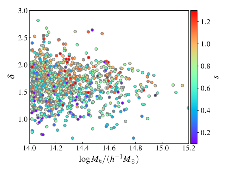
Figure 1: Distribution of 1000 haloes randomly drawn from the twin halo catalogue on the CDM Lagrangian overdensity $\delta$ (linearly extrapolated to $z{=}0$) vs. halo mass $M_{h}$ plane, colour-coded by their peak curvature $s$ according to the colourbar on the right.

To construct a high-purity twin halo catalogue from the paired simulations, we proceed step by step as follows. For each halo with $M_{h}{\geq}10^{14}\,h^{-1}M_{\odot}$ at $z{=}0$ in the ${\nu}0.0$ simulations, we collect all its CDM particles within $r_{200m}$, retrieve their initial positions at $z{=}127$, and compute the barycentre of those particles in the initial density field. We then identify the highest peak within a search radius of $r_{\mathrm{pk}}=200^{1/3}r_{200m}$ about the barycentre as the true density peak that collapsed into that halo. The peak identification is performed over the smoothed density field derived with Nbodykit (Hand et al., 2018). Since the exact density peak also exists in the initial condition of the paired ${\nu}0.4$ simulation, we collect all the CDM particles within $r_{\mathrm{pk}}$ about the peak in the initial condition, and identify its matched counterpart as the halo that inherited the highest fraction of those particles at $z{=}0$ in the ${\nu}0.4$ simulation. To make sure the matches are unique, we repeat the above procedures but start from the haloes in the ${\nu}0.4$ simulations. We only keep the $97\%$ twins that are reproduced during the reversed search in our final twin catalogue, leaving $3458747$ unique halo twins with $M_{h}{\geq}10^{14}\,h^{-1}M_{\odot}$ from the 40 paired simulations.

For the density peak associated with each twins pair, we characterise its peak height by the halo mass $M_{h}$ at $z{=}0$ in the ${\nu}0.0$ simulation to avoid any confusion in the notations (as $\nu$ is reserved for neutrinos rather than peak height). The peak curvature $s$ is computed as

$$s=-\frac{\Delta\,\delta_{\mathrm{cdm}}}{\Delta\,\log M},$$ (3)

where $\Delta\delta_{\mathrm{cdm}}$ is the CDM overdensity difference between $0.75r_{\mathrm{pk}}$ and $r_{\mathrm{pk}}$, and $\Delta\log M$ is the logarithmic differences between the enclosed CDM masses within the two radii. Unlike D08, our curvature definition has an extra minus sign so that steeper peaks have larger positive values of $s$. Figure 1 shows the distribution of 1000 randomly selected haloes on the $M_{h}$ vs. $\delta$ plane, colour-coded by $s$ according to the colourbar on the right, where $\delta$ is the linear theory-extrapolated Lagrangian overdensity at $z{=0}$. Similar to the Fig. 1 in D08, while the overall distribution of $\delta$ centred around the critical overdensity $\delta_{c}{=}1.68$, steeper peaks generally collapsed earlier and have higher values of $\delta$ than the shallower ones. To remove the average halo mass dependence of $s$ in our analysis, we introduce the relative peak curvature $\hat{s}$ as an HAB indicator, defined as

$$\hat{s}=s-\langle s\mid M_{h}\rangle,$$ (4)

where $\langle s|M_{h}\rangle$ is the average curvature as a function of halo mass.

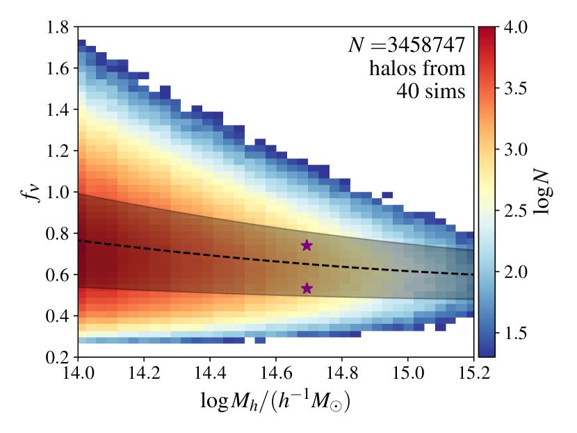
Figure 2: Distribution of all haloes on the neutrino-to-CDM ratio $f_{\nu}$ vs. halo mass $M_{h}$ plane, colour-coded by the logarithmic number of haloes in each cell according to the colourbar on the right. Black dashed line and gray shaded band indicate the mean $f_{\nu}$-$M_{h}$ relation and its $1{-}\sigma$ scatter. The two purple stars denote the two haloes shown in Figure 3.

Inspired by neutrino differential condensation discovered in Yu et al. (2017), we measure the neutrino-to-CDM ratio $f_{\nu}$ for each halo in the ${\nu}0.4$ simulations. In particular, we define $f_{\nu}$ as

$$f_{\nu}\equiv\frac{\Omega_{\mathrm{cdm}}}{\Omega_{\nu}}\cdot\left[\frac{\rho_{\nu}(r)}{\rho_{\mathrm{cdm}}(r)}\right]_{r{=}5{-}12\,\mathrm{Mpc}/h},$$ (5)

where $\Omega_{\mathrm{cdm}}$ ($\Omega_{\nu}$) is the average CDM (neutrino) density of the simulation, and $\rho_{\mathrm{cdm}}$ ($\rho_{\nu}$) is the local CDM (neutrino) density averaged between $r{=}5{-}12\,h^{-1}\mathrm{Mpc}$ around each halo. The radial range is set so that it is below the neutrino free-streaming length $\lambda_{\mathrm{fs}}$ (${\simeq}20\,h^{-1}\mathrm{Mpc}$ for $\Sigma{M_{\nu}}{=}0.4\,\mathrm{ev}$) and the distance scales that we adopt for calculating halo bias. Figure 2 shows the distribution of haloes on the $f_{\nu}$ vs. $M_{h}$ plane, colour-coded by the number of haloes in each 2D cell according to the colourbar on the right. The average neutrino-to-CDM ratio $\langle f_{\nu}|M_{h}\rangle$ deceases slightly with increasing halo mass (black dashed curve), with a mass-dependent scatter $\sigma_{f_{\nu}}(M_{h})$ (gray shaded band). Similar to Equation 4, we define the neutrino excess parameter $\epsilon_{\nu}$ as another indicator of the HAB, so that

$$\epsilon_{\nu}\equiv\frac{f_{\nu}-\langle f_{\nu}\mid M_{h}\rangle}{\sigma_{f_{\nu}}(M_{h})}.$$ (6)

Our peak-based twin halo catalogue has a unique advantage for isolating the subtle effect of massive neutrinos on HAB. Since each twins pair is tied to the same density peak in the initial condition of both ${\nu}0.0$ and ${\nu}0.4$ simulations, we regard them as the same physical object that merely exhibits different behaviors with the massive neutrinos on and off. Therefore, if we measure two separate HAB signals using the relative peak curvature $\hat{s}$ as the indicator in both ${\nu}0.0$ and ${\nu}0.4$ simulations, the difference between $\hat{b}(\hat{s}|{\nu}0.0)$ and $\hat{b}(\hat{s}|{\nu}0.4)$ can only be induced by massive neutrinos. More important, we can now measure $\hat{b}(\epsilon_{\nu}|{\nu}0.0)$, which is the HAB of haloes in the ${\nu}0.0$ simulations, but using their $\epsilon_{\nu}$ in the ${\nu}0.4$ simulations as the HAB indicator. By comparing this HAB signal with that measured directly from the ${\nu}0.4$ simulations $\hat{b}(\epsilon_{\nu}|{\nu}0.4)$, we will be able to ascertain the direct impact of massive neutrinos on HAB.

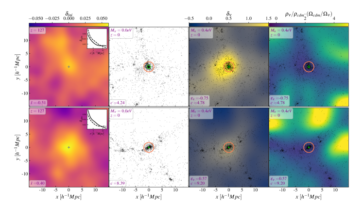
Figure 3: Distributions of the initial CDM overdensity $\delta_{\mathrm{ini}}$ (leftmost), CDM particles (2nd from left), neutrino overdensity $\delta_{\nu}$ (2nd from right), and neutrino-to-CDM density ratio $\rho_{\nu}/\rho_{\mathrm{cdm}}$ (normalised by $\Omega_{\nu}/\Omega_{\mathrm{cdm}}$; rightmost) around two pairs of twin haloes with the same peak height, one collapsed from a shallow ($\hat{s}{=}{-}0.51$; top) density peak and the other steep ($\hat{s}{=}0.40$; bottom). Each panel shows a slice of dimension $30\,h^{-1}\mathrm{Mpc}{\times}30\,h^{-1}\mathrm{Mpc}{\times}12\,h^{-1}\mathrm{Mpc}$ centred on the peak/halo, with the key halo/peak properties annotated in the bottom left corner and the simulation/redshift information in the top left. The maps of $\delta_{\mathrm{ini}}$, $\delta_{\nu}$, and $\rho_{\nu}/\rho_{\mathrm{cdm}}$ are colour-coded according to the respective colourbars on top. The inset panel in each of the leftmost panels shows the radial profiles of the CDM overdensity around the two peaks, with the solid curve corresponding to the $\delta_{\mathrm{ini}}$ distribution shown in the main panel. The inner lime and outter orange circles on the rest of the panels denote the scale radii and $r_{200m}$ of the haloes, respectively.

The left column of Figure 3 shows the initial CDM overdensity $\delta_{\mathrm{ini}}$ at $z{=}127$ surrounding two density peaks with equal peak height, one with a shallow ($\hat{s}{=}{-}0.51$; top) curvature and the other steep ($\hat{s}{=}0.40$; bottom). In each inset panel, we compare the 1D overdensity profiles of the two peaks, with the profile of that shown in the main panel indicated by the solid curve. Each peak subsequently collapsed into the twin haloes in the ${\nu}0.0$ (second column) and ${\nu}0.4$ (third column) simulations, with their halo radii $r_{200m}$ and characteristic scales $r_{s}$ indicated by the outter orange and inner lime circles, respectively. The distributions of CDM particles (black dots) are very similar between the two simulations, and the neutrino overdensity $\delta_{\nu}$ follows the CDM distribution on large scales in the ${\nu}0.4$ simulation. The rightmost column shows the neutrino-to-CDM ratio $\rho_{\nu}/\rho_{\mathrm{cdm}}$ (normalised by $\Omega_{\nu}/\Omega_{\mathrm{cdm}}$) surrounding the halos formed in the ${\nu}0.4$ simulation. Each panel of Figure 3 corresponds to a region of $30\,h^{-1}\mathrm{Mpc}{\times}30\,h^{-1}\mathrm{Mpc}$ size centred on the peak/halo, projected along a $12\,h^{-1}\mathrm{Mpc}$ length in the $z$-direction. The distributions of $\delta_{\mathrm{ini}}$, $\delta_{\nu}$, and $\rho_{\nu}/\rho_{\mathrm{cdm}}$ are colour-coded according to the respective colourbars on top. As expected, the steep peak collapsed into haloes with higher concentration than the shallow one. The concentrations of haloes in the ${\nu}0.4$ simulation is in general higher than those in the ${\nu}0.0$ one (Brandbyge et al., 2010; Villaescusa-Navarro et al., 2013; Lazeyras et al., 2021); This overall concentration difference is removed from the HAB comparison by using $\hat{c}$. More interestingly, within the ${\nu}0.4$ simulation, the halo formed from the high-$\hat{s}$ peak has a larger $\epsilon_{\nu}{=}0.57$ than that from the low-$\hat{s}$ one (${-}0.75$). This signals the existence of a positive correlation between $\hat{s}$ and $\epsilon_{\nu}$, hence a potential neutrino-induced HAB.

3 Results

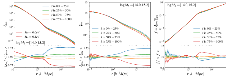
Figure 4: 3D cross-correlation functions between haloes and CDM $\xi_{\mathrm{hm}}$ (left), haloes and neutrinos $\xi_{\mathrm{h\nu}}$ (middle), and the ratio between the two correlation functions $\xi_{\mathrm{h\nu}}/\xi_{\mathrm{hm}}$ (right), for haloes divided into four quartiles by their relative peak curvature $\hat{s}$ (listed in the top right corner of the left panel). Solid and dashed curves show the measurements from the ${\nu}0.0$ and ${\nu}0.4$ simulations, respectively. The bottom panels show the ratio between profiles of the individual quartiles to that of the overall population.

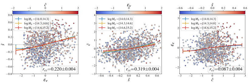
Figure 5: Pairwise correlations between $\epsilon_{\nu}$, $\hat{s}$, and $\hat{c}$. In each panel, circles represent 1000 randomly selected haloes from the twin halo catalogue on the axis plane defined by two parameters, colour-coded by their values of the third parameter. Blue, gold, and red curves show the mean relations between the two axis parameters for haloes within the three mass bins listed in the top right corner, while the overall Pearson’s correlation coefficient $r_{\mathrm{cc}}$ and its $1{-}\sigma$ uncertainty are listed in bottom right.

To ascertain the correlation between $\hat{s}$ and $\epsilon_{\nu}$, we show the 3D cross-correlation functions between haloes and CDM ($\xi_{\mathrm{hm}}$; left), haloes and massive neutrinos ($\xi_{\mathrm{h\nu}}$; middle), and the ratio between the two ($\xi_{\mathrm{h\nu}}/\xi_{\mathrm{hm}}$; right), for haloes in different quartiles of $\hat{s}$ in Figure 4. In each panel, the top main panel shows the profile comparison between four quartiles in $\hat{s}$, while the bottom sub-panel highlights their differences using the ratio between each quartile and the overall profile of that mass bin. The uncertainty bands are computed by Jackknife resampling over the 40 independent simulations.

In the left panel of Figure 4, solid and dashed curves are the $\xi_{\mathrm{hm}}$ measurements from the ${\nu}0.0$ and ${\nu}0.4$ simulations, respectively. The $\xi_{\mathrm{hm}}$ profiles exhibit the typical one- and two-halo components that can be described using the combination of NFW (Navarro et al., 1997) profiles and biased versions of the matter-matter auto-correlation function $\xi_{\mathrm{mm}}$ (Hayashi & White, 2008; Zu et al., 2014). A strong HAB effect is present in both simulations, as shown by the bottom subpanel, where haloes collapsed from steep peaks (red and brown) are more concentrated within the halo radius and have lower relative clustering amplitude on scales above $15\,h^{-1}\mathrm{Mpc}$ than their shallow-peak counterparts (blue and green). However, The HAB in the ${\nu}0.4$ (dashed) simulations is slightly weaker than that in the ${\nu}0.0$ ones (solid), in that the relative clustering of the steepest (shallowest) quartile is lower (higher) in ${\nu}0.4$ than in ${\nu}0.0$ simulations. This weakening of $\hat{s}$-indicated HAB in the ${\nu}0.4$ simulations, albeit very small in amplitude, constitutes our first evidence that the HAB is modified by the presence of massive neutrinos. The middle panel of Figure 4 is similar to the left, but for the $\xi_{\mathrm{h\nu}}$ profiles measured from the ${\nu}0.4$ simulations. Consistent with the results from LoVerde & Zaldarriaga (2014), the “neutrino haloes” extend to a much greater radius than the virial radius of the CDM haloes. Interestingly, the $\xi_{\mathrm{h\nu}}$ profiles exhibit its own HAB phenomenon analogous to the CDM version — the steep density peaks attract more concentrated “neutrino haloes” that exhibit lower relative clustering of neutrinos on large scales than the shallow ones. This to our knowledge is the first detection of the “neutrino halo” assembly bias effect in simulations.

The right panel of Figure 4 shows the ratio profiles between $\xi_{\mathrm{h\nu}}$ and $\xi_{\mathrm{hm}}$ in the ${\nu}0.4$ simulations. Within $r_{200m}$, the ratio profile rises sharply as ${\simeq}r^{3/2}$, but levels off as ${\simeq}r^{2/3}$ beyond $r_{200m}$. Though not shown here, the ratio profile should reach a plateau of unity at scales ${\gg}\lambda_{\mathrm{fs}}{\simeq}20\,h^{-1}\mathrm{Mpc}$ where neutrinos follow CDM. More important, the bottom panel reveals that $\hat{s}$ indeed correlates with the neutrino-to-CDM ratio on quasi-linear scales. In particular, haloes collapsed from the steepest (shallowest) quartile exhibit a ${\sim}10\%$ enhancement (deficit) in their neutrino-to-CDM ratio between $r_{200m}$ and $\lambda_{\mathrm{fs}}$ compared to the average population. Therefore, we expect a positive correlation between $\hat{s}$ and the previously defined neutrino excess parameter $\epsilon_{\nu}$. Given that massive neutrinos seem to cause an impact on the $\hat{s}$-indicated HAB (left panel of Figure 4), such a $\hat{s}$-$\epsilon_{\nu}$ correlation implies that the impact on the $\epsilon_{\nu}$-indicated HAB would likely be greater.

While being theoretically informative, neither $\hat{s}$ nor $\epsilon_{\nu}$ is an observable quantity. As of now, concentration remains one of the most promising observable indicators of HAB Zu et al. (2021) and it is thus imperative that we explore the neutrino impact on the $\hat{c}$-indicated HAB. Figure 5 presents the pairwise correlations between the three HAB indicators. For each panel of $x$ vs. $y$, circles represent the $x$ and $y$ values of 1000 individual haloes randomly drawn from the twin halo catalogue in the ${\nu}0.4$ simulation, each colour-coded by the value of the third indicator according to the colourbar on top. The three coloured curves are the mean relations $\langle y|x\rangle$ calculated for the three halo mass bins listed in the legend, while the overall cross-correlation coefficient $r_{\mathrm{cc}}$ is annotated in the bottom right with its $1{-}\sigma$ uncertainty. Overall, the three indicators all correlate with one another, with little dependence on halo mass. The correlation between $\hat{s}$ and $\hat{c}$ (middle panel) is the strongest among the three pairs with $r_{\mathrm{cc}}{=}0.319$. The correlation between $\hat{s}$ and $\epsilon_{\nu}$ are reasonably strong with $r_{\mathrm{cc}}{=}0.220$, consistent with our expectation from the right panel of Figure 4. Meanwhile, the correlation between $\epsilon_{\nu}$ and $\hat{c}$ is significantly detected but with a weak strength of $r_{\mathrm{cc}}{=}0.087{\pm}0.004$. Although the intrinsic correlation between $\epsilon_{\nu}$ and $\hat{c}$ ought to be higher, because the measurement of $\hat{c}$ is subject to shot noise (see Wang et al., 2023, for potential improvements), the measurement error in real observations can only be larger (Zu et al., 2017).

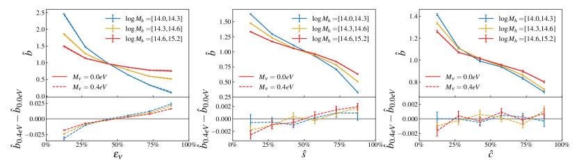
Figure 6: HAB comparison between the ${\nu}0.0$ (solid curves) and ${\nu}0.4$ (dashed curve) simulations, using the neutrino excess $\epsilon_{\nu}$, relative peak curvature $\hat{s}$, relative concentration $\hat{c}$ as indicators in the left, middle, and right panel, respectively. The HAB is characterised by the relative bias $\hat{b}$ as a function of the indicator divided into six sextiles. Blue, gold, and red curves indicate the results from the three halo mass bin of $\log M_{h}{=}[14.0,14.3]$, $[14.3,14.6]$, and $[14.6,15.2]$, respectively. Each bottom subpanel shows the difference between the two sets of $\hat{b}$ functions in the ${\nu}0.0$ and ${\nu}0.4$ simulations. All errorbars are jackknife uncertainties from the 40 independent simulations.

Finally, we show the impact of massive neutrinos on the HABs indicated by neutrino excess $\epsilon_{\nu}$ (left), relative peak curvature $\hat{s}$ (middle), and relative halo concentration $\hat{c}$ (right) in Figure 6, the key result of this letter. In each panel of indicator $x$ (divided into sextiles), the main panel compares the HABs as measured by $\hat{b}(x|M_{h})$ between the ${\nu}0.0$ (solid curves) and ${\nu}0.4$ (dashed curves) simulations, in three different mass bins of $\log M_{h}{=}[14.0,14.3]$ (blue), $[14.3,14.6]$ (gold), and $[14.6,15.2]$ (red). The halo bias $b$ is measured from $\xi_{\mathrm{hm}}/\xi_{\mathrm{mm}}$ on scales between $15\,h^{-1}\mathrm{Mpc}$ and $30\,h^{-1}\mathrm{Mpc}$ (see the left panel of Figure 4), with Jackknife errorbars estimated from the 40 simulations. The discrepancy between the two sets of HABs is more clearly seen in the bottom subpanel, which shows $\Delta\hat{b}(x|M_{h})=\hat{b}(x|M_{h})_{{\nu}0.4}-\hat{b}(x|M_{h})_{{\nu}0.0}$.

When $\epsilon_{\nu}$ is used as the indicator (left panel of Figure 6), the HAB strength is significantly weakened in the presence of massive neutrinos. Combining the three halo mass bins, the relative bias of the least neutrino-rich sextile of haloes is reduced by $0.033{\pm}{0.003}$, while that of the most neutrino-rich sextile of haloes is enhanced by $0.028{\pm}{0.001}$. The neutrino effect decreases by an order of magnitude when $\hat{s}$ is used as the HAB indicator (middle panel), in which case the $\Delta\hat{b}$ of the steepest (shallowest) sextile of density peaks becomes ${-}0.00105{\pm}{0.00194}$ (${}0.00207{\pm}{0.00072}$). Unfortunately, these $0.1{-}2$ per-cent level differences are currently only detectable in simulations, especially given that the upper bound on $\Sigma{M_{\nu}}$ is well below $0.4\,\mathrm{ev}$ (Di Valentino et al., 2021).

When $\hat{c}$ is adopted for HAB detection (right panel of Figure 6), the effect of massive neutrinos completely diminishes, with $\Delta\hat{b}$ consistent with zero across all sextiles of relative concentration. This is somewhat expected given that $\hat{c}$ barely correlates with $\epsilon_{\nu}$, the underlying driver of neutrino-induced HAB. This null detection of neutrino effects is also consistent with the result of Lazeyras et al. (2021), despite the difference in concentration measurement and halo catalogues. Therefore, Figure 6 elucidates the impact of massive neutrinos on concentration-indicated HAB — massive neutrinos are able to modify the HAB signal predicted by massless neutrino simulations, as long as haloes are divided by their local neutrino-to-CDM ratio or the curvature of their initial density peaks.

4 Conclusion

In this letter, we elucidate the impact of massive neutrinos on the halo assembly bias (HAB) using a large suite of massless and massive neutrino ($\Sigma{M_{\nu}}{=}0.4\,\mathrm{ev}$) simulations from Quijote. By tracing haloes back to their density peaks in the initial condition shared by both types of simulations, we construct a twin halo catalogue where each twins pair is characterised by their relative concentration $\hat{c}$, relative peak curvature $\hat{s}$, and relative neutrino-to-CDM ratio $\epsilon_{\nu}$.

Using the relative halo bias $\hat{b}$ to quantify the strength of HAB, we demonstrate that the massive neutrinos could cause a two per cent-level impact on the HAB effect compared to that predicted by the massless neutrino simulations, if $\epsilon_{\nu}$ is used as the HAB indicator. Since $\hat{s}$ is strongly correlated with $\epsilon_{\nu}$, the neutrino-induced HAB remains discernible at the $0.1$-per cent level when $\hat{s}$ is used as the indicator. However, the minuscule correlation between $\hat{c}$ and $\epsilon_{\nu}$ renders the $\hat{c}$-indicated HABs indistinguishable between the massless and massive neutrino simulations — a null effect consistent with previous works (e.g., Lazeyras et al., 2021).

In the future, we plan to explore if there exist halo observables that can potentially correlate better with $\epsilon_{\nu}$ than $\hat{c}$, thereby yielding detectable neutrino-induced HAB signals, at least in the simulations. Although extremely challenging, an observational detection of the neutrino-induced HAB with next-generation galaxy surveys, including the Dark Energy Spectroscopic Instrument (DESI; DESI Collaboration et al., 2022), Prime Focus Spectrograph (PFS; Takada et al., 2006), Roman Space Telescope (Roman; Spergel et al., 2015), EUCLID (Laureijs et al., 2011), and the Chinese Survey Space Telescope (CSST; Gong et al., 2019), would provide an independent path to measuring $\Sigma{M_{\nu}}$ using the LSS information beyond the linear power spectrum (Bayer et al., 2022),

Data Availability

The Quijote simulation data underlying this article are publicly available via https://github.com/franciscovillaescusa/Quijote-simulations.

References

- Alam et al. (2017) Alam S., et al., 2017, MNRAS, 470, 2617
- Bardeen et al. (1986) Bardeen J. M., Bond J. R., Kaiser N., Szalay A. S., 1986, ApJ, 304, 15
- Bayer et al. (2022) Bayer A. E., Banerjee A., Seljak U., 2022, Phys. Rev. D, 105, 123510
- Behroozi et al. (2013) Behroozi P. S., Wechsler R. H., Wu H.-Y., 2013, ApJ, 762, 109
- Bond et al. (1991) Bond J. R., Cole S., Efstathiou G., Kaiser N., 1991, ApJ, 379, 440
- Brandbyge et al. (2010) Brandbyge J., Hannestad S., Haugbølle T., Wong Y. Y. Y., 2010, J. Cosmology Astropart. Phys., 2010, 014
- Brinckmann et al. (2019) Brinckmann T., Hooper D. C., Archidiacono M., Lesgourgues J., Sprenger T., 2019, J. Cosmology Astropart. Phys., 2019, 059
- Contreras et al. (2021) Contreras S., Chaves-Montero J., Zennaro M., Angulo R. E., 2021, MNRAS, 507, 3412
- Cuesta et al. (2016) Cuesta A. J., Niro V., Verde L., 2016, Physics of the Dark Universe, 13, 77
- DESI Collaboration et al. (2022) DESI Collaboration et al., 2022, AJ, 164, 207
- Dalal et al. (2008) Dalal N., White M., Bond J. R., Shirokov A., 2008, ApJ, 687, 12
- Di Valentino et al. (2021) Di Valentino E., Gariazzo S., Mena O., 2021, Phys. Rev. D, 104, 083504
- Dvorkin et al. (2019) Dvorkin C., et al., 2019, BAAS, 51, 64
- Gao & White (2007) Gao L., White S. D. M., 2007, MNRAS, 377, L5
- Gao et al. (2005) Gao L., Springel V., White S. D. M., 2005, MNRAS, 363, L66
- Giusarma et al. (2016) Giusarma E., Gerbino M., Mena O., Vagnozzi S., Ho S., Freese K., 2016, Phys. Rev. D, 94, 083522
- Gong et al. (2019) Gong Y., et al., 2019, ApJ, 883, 203
- Hand et al. (2018) Hand N., Feng Y., Beutler F., Li Y., Modi C., Seljak U., Slepian Z., 2018, AJ, 156, 160
- Harker et al. (2006) Harker G., Cole S., Helly J., Frenk C., Jenkins A., 2006, MNRAS, 367, 1039
- Hayashi & White (2008) Hayashi E., White S. D. M., 2008, MNRAS, 388, 2
- Ichiki & Takada (2012) Ichiki K., Takada M., 2012, Phys. Rev. D, 85, 063521
- Ivanov et al. (2020) Ivanov M. M., Simonović M., Zaldarriaga M., 2020, Phys. Rev. D, 101, 083504
- Jing et al. (2007) Jing Y. P., Suto Y., Mo H. J., 2007, ApJ, 657, 664
- Kaiser (1984) Kaiser N., 1984, ApJ, 284, L9
- Laureijs et al. (2011) Laureijs R., et al., 2011, arXiv e-prints, p. arXiv:1110.3193
- Lazeyras et al. (2021) Lazeyras T., Villaescusa-Navarro F., Viel M., 2021, J. Cosmology Astropart. Phys., 2021, 022
- Lesgourgues & Pastor (2006) Lesgourgues J., Pastor S., 2006, Phys. Rep., 429, 307
- Li et al. (2008) Li Y., Mo H. J., Gao L., 2008, MNRAS, 389, 1419
- Lin et al. (2016) Lin Y.-T., Mandelbaum R., Huang Y.-H., Huang H.-J., Dalal N., Diemer B., Jian H.-Y., Kravtsov A., 2016, ApJ, 819, 119
- Lin et al. (2022) Lin Y.-T., Miyatake H., Guo H., Chiang Y.-K., Chen K.-F., Lan T.-W., Chang Y.-Y., 2022, A&A, 666, A97
- LoVerde & Zaldarriaga (2014) LoVerde M., Zaldarriaga M., 2014, Phys. Rev. D, 89, 063502
- Mao et al. (2018) Mao Y.-Y., Zentner A. R., Wechsler R. H., 2018, MNRAS, 474, 5143
- Miyatake et al. (2016) Miyatake H., More S., Takada M., Spergel D. N., Mandelbaum R., Rykoff E. S., Rozo E., 2016, Phys. Rev. Lett., 116, 041301
- Navarro et al. (1997) Navarro J. F., Frenk C. S., White S. D. M., 1997, ApJ, 490, 493
- Palanque-Delabrouille et al. (2020) Palanque-Delabrouille N., Yèche C., Schöneberg N., Lesgourgues J., Walther M., Chabanier S., Armengaud E., 2020, J. Cosmology Astropart. Phys., 2020, 038
- Planck Collaboration et al. (2020) Planck Collaboration et al., 2020, A&A, 641, A6
- Prada et al. (2012) Prada F., Klypin A. A., Cuesta A. J., Betancort-Rijo J. E., Primack J., 2012, MNRAS, 423, 3018
- Press & Schechter (1974) Press W. H., Schechter P., 1974, ApJ, 187, 425
- Salcedo et al. (2018) Salcedo A. N., Maller A. H., Berlind A. A., Sinha M., McBride C. K., Behroozi P. S., Wechsler R. H., Weinberg D. H., 2018, MNRAS, 475, 4411
- Sheth & Tormen (1999) Sheth R. K., Tormen G., 1999, MNRAS, 308, 119
- Sheth & Tormen (2004) Sheth R. K., Tormen G., 2004, MNRAS, 350, 1385
- Spergel et al. (2015) Spergel D., et al., 2015, arXiv e-prints, p. arXiv:1503.03757
- Sunayama et al. (2022) Sunayama T., More S., Miyatake H., 2022, arXiv e-prints, p. arXiv:2205.03277
- Takada et al. (2006) Takada M., Komatsu E., Futamase T., 2006, Phys. Rev. D, 73, 083520
- Vagnozzi et al. (2017) Vagnozzi S., Giusarma E., Mena O., Freese K., Gerbino M., Ho S., Lattanzi M., 2017, Phys. Rev. D, 96, 123503
- Villaescusa-Navarro et al. (2013) Villaescusa-Navarro F., Bird S., Peña-Garay C., Viel M., 2013, J. Cosmology Astropart. Phys., 2013, 019
- Villaescusa-Navarro et al. (2020) Villaescusa-Navarro F., et al., 2020, ApJS, 250, 2
- Wang et al. (2023) Wang K., Mo H. J., Chen Y., Schaye J., 2023, arXiv e-prints, p. arXiv:2310.00200
- Wechsler et al. (2006) Wechsler R. H., Zentner A. R., Bullock J. S., Kravtsov A. V., Allgood B., 2006, ApJ, 652, 71
- Wong (2011) Wong Y. Y. Y., 2011, Annual Review of Nuclear and Particle Science, 61, 69
- Yang et al. (2006) Yang X., Mo H. J., van den Bosch F. C., 2006, ApJ, 638, L55
- Yu et al. (2017) Yu H.-R., et al., 2017, Nature Astronomy, 1, 0143
- Zu et al. (2014) Zu Y., Weinberg D. H., Rozo E., Sheldon E. S., Tinker J. L., Becker M. R., 2014, MNRAS, 439, 1628
- Zu et al. (2017) Zu Y., Mandelbaum R., Simet M., Rozo E., Rykoff E. S., 2017, MNRAS, 470, 551
- Zu et al. (2021) Zu Y., et al., 2021, MNRAS, 505, 5117
- Zu et al. (2022) Zu Y., et al., 2022, MNRAS, 511, 1789