KAgoshima Galactic Object survey with Nobeyama 45-metre telescope by Mapping in Ammonia lines (KAGONMA): Discovery of parsec-scale CO depletion in the Canis Major star-forming region

Abstract

In observational studies of infrared dark clouds, the number of detections of CO freeze-out onto dust grains (CO depletion) at pc-scale is extremely limited, and the conditions for its occurrence are, therefore, still unknown. We report a new object where pc-scale CO depletion is expected. As a part of Kagoshima Galactic Object survey with Nobeyama 45-m telescope by Mapping in Ammonia lines (KAGONMA), we have made mapping observations of NH₃ inversion transition lines towards the star-forming region associated with the CMa OB1 including IRAS 07077–1026, IRAS 07081–1028, and PGCC G224.28–0.82. By comparing the spatial distributions of the NH₃ (1,1) and C¹⁸O ($J$=1–0), an intensity anti-correlation was found in IRAS 07077–1026 and IRAS 07081–1028 on the $\sim$1 pc scale. Furthermore, we obtained a lower abundance of C¹⁸O at least in IRAS 07077–1026 than in the other parts of the star-forming region. After examining high density gas dissipation, photodissociation, and CO depletion, we concluded that the intensity anti-correlation in IRAS 07077–1026 is due to CO depletion. On the other hand, in the vicinity of the centre of PGCC G224.28–0.82, the emission line intensities of both the NH₃ (1,1) and C¹⁸O ($J$=1–0) were strongly detected, although the gas temperature and density were similar to IRAS 07077–1026. This indicates that there are situations where C¹⁸O ($J$=1–0) cannot trace dense gas on the pc scale and implies that the conditional differences that C¹⁸O ($J$=1–0) can and cannot trace dense gas are unclear.

1 Introduction

Star formation is known to occur in cold, dense molecular clouds. In general, molecular clouds have a temperature of $\sim$10 K, a volume density of about 10² – 10⁵ cm^-3 (e.g., Dame et al., 2001; Bergin & Tafalla, 2007), and are mostly composed of molecular hydrogen. The basic approach to measuring the mass of molecular clouds is to count the number of hydrogen molecules along the line-of-sight, called the H₂ column density, $N$(H₂). However, radiation from molecular hydrogen, which is most abundant in molecular clouds, can only be detected from gas with a temperature above 80 K (Togi & Smith, 2016). This means that it is not possible to observe H₂ emission from low-temperature regions directly related to the star-forming activity. Therefore, it is often used to determine the column density of CO molecules, $N$(CO), from the emission of CO isotopologues (e.g., ¹²CO, ¹³CO, and C¹⁸O), which are the most abundant molecules after H₂, and use the [CO]/[H₂] abundance ratio to measure $N$(H₂) indirectly.

$N$(CO) and $N$(H₂) are not necessarily linear relationships (e.g., Frerking et al., 1982; Pineda et al., 2008; Ripple et al., 2013; Wang et al., 2019). In the relatively low temperature ($T$ $<$ 20 K) and high volume density ($n$(H₂) $>$ 10⁴ cm^-3) regions, CO molecules freeze out and adsorb onto dust grains has been reported (e.g., Willacy et al., 1998; Tafalla et al., 2002). In the case of CO freeze-out onto dust grains, low-$J$ lines of rare CO isotopologues such as C¹⁸O or C¹⁷O cannot trace the dense and cold gas (e.g., Caselli et al., 1999). This phenomenon, which is called CO freeze-out onto dust grains or depletion (hereafter CO depletion), is important for understanding the chemistry of molecular clouds because it not only affects the gas-phase chemistry but also promotes the surface reaction in dust grains.

CO depletion has been actively studied in nearby low-mass star-forming regions (e.g., Willacy et al., 1998; Caselli et al., 1999; Kramer et al., 1999; Bergin & Tafalla, 2007). They have reported that CO depletion is frequently detected in starless cores at $T$ $<$ 20 K and $n$(H₂) $>$ 3 $\times$ $10^{4}$ cm^-3, and the spatial scale is mostly comparable to the size of the molecular cloud core ($\sim$0.05 pc). This is because the free fall timescale and the depletion timescale coincide at the typical density of molecular cloud cores ($\simeq$10⁴ cm^-3).

In recent years, a small number of sources with pc-scale CO depletion have been reported from mapping observations of the CO isotopologue lines Hernandez et al. (2011); Jiménez-Serra et al. (2014); Feng et al. (2016a, 2020); Gong et al. (2018); Sabatini et al. (2019, 2022); Lewis et al. (2021). In infrared dark clouds (IRDCs), which have higher densities than low-mass star-forming regions, pc-scale CO depletion is expected to be a common event; pc-scale CO depletion has been reported over a wide mass range, from low-mass IRDC, the Serpens filament (20 – 66 $\MO$, Roccatagliata et al., 2015; Gong et al., 2018) to IRDCs that massive enough to form high-mass stars (e.g., Sabatini et al., 2019; Feng et al., 2020). In low-mass star-forming regions, CO depletion occurs in cloud cores, whereas in IRDCs CO depletion occurs not only in cloud cores but also in clumps and filaments. However, previous studies are biased towards high-mass IRDCs that fulfil an empirical threshold for high-mass star formation, $M(r)>870\ \MO$ (radius/pc)^1.33 (Kauffmann & Pillai, 2010). To better understand pc-scale CO depletion, more low-mass/intermediate-mass sources with pc-scale CO depletion are required.

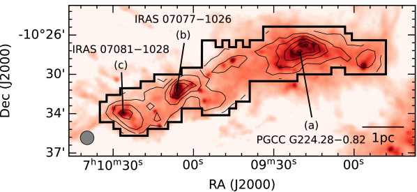
Figure 1: The NH₃ integrated intensity map of KAG71 in contours over the Herschel/SPIRE 250  dust continuum image. The black polygon outlines the mapping area of the NH₃ observations. The labels (a) – (c) indicate the positions for the spectra of figures 2-(a) to (c). The lowest contour and contour steps are 0.2 K km s^-1 and 0.4 K km s^-1, respectively. The Nobeyama 45 m beam size at 23 GHz is indicated by the grey filled circle shown in the lower left corner. (Color online)

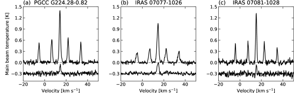
Figure 2: Panel (a) – (c) : The spectra in the NH₃ (1,1) (top) and (2,2) (bottom) at the position assigned in figure 1 with the same labels. (Color online)

We focus on NH₃ molecular species. This molecule species is a good gas tracer in dense and cold regions, where star formation can occur (e.g., Myers & Benson, 1983). The critical density of the NH₃ inversion transition lines are $\sim$2.0 $\times$ 10³ cm^-3 (Shirley, 2015), which is comparable to that of the C¹⁸O ($J$=1–0) lines ($\sim$2.0 $\times$ 10³ cm^-3, Pety et al., 2017). These molecule lines are a good combination for comparing the properties of gases other than density differences. Previous studies of NH₃ lines reported that NH₃ is a depletion-resistant species and does not freeze out only in cold and dense gas regions ($T$ $<$ 20 K, $n\geq 10^{5}$ cm^-3), where carbon-bearing molecules have already been frozen out onto dust grains (e.g., Tafalla et al., 2002; Crapsi et al., 2007; Sipilä et al., 2019). Comparing the spatial distributions of NH₃ and C¹⁸O may be able to detect pc-scale CO depletion. If this comparison can detect pc-scale CO depletion, it would be possible to separate the line-of-sight components, which is difficult to do with dust emission comparisons.

We observed NH₃ lines towards a star-forming region associated with the Canis Major (CMa) OB1 region. Figure 1 shows the our observed area superimposed on the Herschel (Pilbratt et al., 2010) 250  dust continuum image. This star-forming region is one of the targets of KAGONMA (Kagoshima Galactic Object survey with Nobeyama 45-metre telescope by Mapping in Ammonia lines) survey project (Murase et al., 2022; Kohno et al., 2022, 2023), which is identified as KAGONMA 71 (hereafter KAG71). KAG71 corresponds to Canis Major Group 00 (Fischer et al., 2016) and Hi-GAL $l$ = 224^∘ region main filament (Olmi et al., 2016). KAG71 contains Planck Catalogue of Galactic Cold Clumps (PGCC: Planck Collaboration et al., 2016a) G224.28–0.82, IRAS 07077–1026, and IRAS 07081–1028. Elia et al. (2013) reported that the dust temperature, derived from the Herschel dust continuum data, was between 11 K and 13 K in most of this region. They also identified compact objects such as cores and clumps, and reported that most of the compact objects were associated with protostars. Previous studies have reported cluster formations (Fischer et al., 2016; Sewiło et al., 2019) and identified the outflows from protostars associated with clusters (Sewiło et al., 2019; Lin et al., 2021). This suggests that our target is a very young and active star-forming region. The distance to CMa OB1 is estimated by various methods and is still uncertain: 1150 pc based on the colour magnitude diagram (Clariá, 1974), 990 $\pm$ 50 pc based on $uvby\beta$ photometry (Kaltcheva & Hilditch, 2000), and 1100 pc based on kinematic distances derived from ¹³CO ($J$=1–0) data (Kim et al., 2004). There are several molecular clouds in the line-of-sight to CMa OB1. Their distances are individually estimated from kinematic distances using CO ($J$=1–0) data (Elia et al., 2013), and a cloud corresponding to KAG71 is at a distance of 900 pc. We adopt 900 pc to be consistent with previous studies (Elia et al., 2013; Sewiło et al., 2019).

This paper is organised as follows: in section 2, we describe the set-up of our observations, data reduction, and archival data sets. In section 3, we present the results of the spatial distribution of the NH₃ emission, the C¹⁸O ($J$=1–0) emission and the dust continuum emission. The difference of spatial distributions is discussed and possible causes are described in section 4. In section 5, we summarise our results and conclusions.

Table 1: The HPBW and main-beam efficiency at each polarisation for each observation season.

season	HPBW (RHCP)	HPBW (LHCP)	$\eta_{\mathrm{mb}}$ (RHCP)	$\eta_{\mathrm{mb}}$ (LHCP)
2015-2016 2016-2017	74.4 $\pm$ 0.3	73.9 $\pm$ 0.3	83% $\pm$ 4%	84% $\pm$ 4%
2017-2018 2018-2019	73$\pm$ 1	72$\pm$ 1	84% $\pm$ 2%	83% $\pm$ 2%

2 Observations and data

2.1 NH₃ and H₂O Maser Observations

We made mapping observations covering an area of 26 $\times$ 10 area (figure 1) with the Nobeyama 45 m radio telescope from 2016 December to 2019 May. These observations used a high electron mobility transistor receiver, H22, and an auto-correlation spectrometer, the Spectral Analysis Machine for the 45 m telescope, SAM45 (Kuno et al., 2011). The metastable NH₃ inversion transitions at ($J,K$) = (1,1), (2,2), and (3,3), and H₂O maser were observed simultaneously in both circular polarisations. We observed 295 positions on a 37.5 grid in the equatorial coordinates and the three-ON points position-switch observations. The half-power beam width (HPBW) varies slightly between the observing seasons and between the two circular polarisations (see table 1). We refer to 75 (corresponding to 0.33 pc at 900 pc), which is twice the grid size, as the effective beam size of the map instead of the HPBW. The OFF position was taken at ($\alpha_{\mathrm{J2000}},\delta_{\mathrm{J2000}}$) = (07:09:20.31, $-$10:27:55.35), where no NH₃ emission lines and no H₂O maser emission line were detected. The pointing accuracy was checked every hour using the H₂O maser sources associated with IK Tau, VY CMa, and Z Pup, and was within 7. The rest frequencies NH₃ ($J,K$) = (1,1), (2,2), (3,3), and H₂O maser are 23.694495 GHz, 23.722633 GHz, 23.870129 GHz, and 22.235080 GHz, respectively. The bandwidth and frequency resolution are 62.5 MHz and 15.26 kHz, respectively, corresponding to 400 km s^-1 and 0.19 km s^-1 at the NH₃ (1,1) frequency. During the observations, the system noise temperature was between 100 K and 1000 K, or typically 200 K. The antenna temperature ($T_{\mathrm{a}}^{*}$) was calibrated by the chopper wheel method.

Data reductions were performed using the Java NEWSTAR software package developed at the Nobeyama Radio Observatory (NRO). Baseline correction was performed with a third-order polynomial for emission-free channels. The main beam efficiency ($\eta_{\mathrm{mb}}$) at 23 GHz is different for each observation season and polarisation (see table 1). We used the mean value, 83.5%, as $\eta_{\mathrm{mb}}$ for the whole observation season to convert from $T_{\mathrm{a}}^{*}$ to $T_{\mathrm{mb}}$. To check the consistency and reduce the noise level, we observed one or more times at the same position and averaged both polarisation data with a weight of 1/rms². To reduce the noise level, we also smoothed the NH₃ data to a velocity resolution of 0.38 km s^-1. The resulting rms noise level (hereafter $\sigma_{\mathrm{rms}}$) is typically 0.027 K on the $T_{\mathrm{mb}}$ scale. For the H₂O maser observations, a conversion factor of 2.8 Jy K^-1 was used to convert the antenna temperature to flux density.

2.2 Archival Data / Catalogue

We used the ¹²CO ($J$=1–0) and C¹⁸O ($J$=1–0) data cubes obtained with the Mopra 22 m telescope (Olmi et al., 2016). The beam size and velocity resolution are 38 and 0.09 km s^-1, respectively. We used the main beam efficiency of 0.42 (Ladd et al., 2005) measured at 115 GHz to convert the antenna temperature to the brightness temperature. Baseline correction was performed with a first-order polynomial for emission-free channels. To reduce the noise level, we smoothed over six spectral channels and the resulting velocity resolution is $\simeq$0.55 km s^-1. We have also produced regridded data with a grid size of 14 for comparison with the Herschel dust continuum data. The mean rms noise of the 14 data is 0.39 K for ¹²CO and 0.18 K for C¹⁸O on the $T_{\mathrm{mb}}$ scale, respectively. Although the observed area of the Mopra data does not cover the whole of our NH₃ observed area, the uncovered area is small; about 2 at the eastern and western edges of our area.

In order to understand the C¹⁸O distribution in the entire NH₃ observed area, we also used the C¹⁸O ($J$=1–0) data cube from FOREST Unbiased Galactic plane imaging survey (FUGIN: Umemoto et al., 2017), which is one of the legacy projects of the NRO. The FUGIN ¹²CO ($J$=1–0) data cube was also used to check the intensity consistency between the Mopra data and the FUGIN data. The effective beam size and velocity resolution are 20 and 1.3 km s^-1 respectively. The mean rms noise is 3.6 K for ¹²CO and 1.5 K for C¹⁸O on the $T_{\mathrm{mb}}$ scale, respectively. We smoothed the C¹⁸O data to become its beam size of 75 and regridded it to a grid size of 37.5 to match our NH₃ maps using the Astronomical Image Processing System (AIPS) software. The resulting mean rms noise is 0.25 K.

The original FUGIN C¹⁸O data are not sensitive enough, and the Mopra CO isotopologue lines data are smaller than our observed area. This makes it difficult to compare the intensity distributions of the C¹⁸O line and the NH₃ line. In this paper, we used the smoothed FUGIN C¹⁸O data to compare the line intensity distribution between C¹⁸O and NH₃, and the Mopra data for comparison with dust properties. The Mopra ¹²CO intensity is about 30% higher than the FUGIN ¹²CO intensity, the C¹⁸O intensities agree within 5%. We discuss the effects of the different ¹²CO intensities on the physical parameters in appendix A.

To understand the spatial distribution and physical conditions of the dust, we used the Herschel dust continuum data from 160 $\micron$ to 500 $\micron$ with the identification numbers (OBSID) 1342220650 and 1342220651. These were obtained from the Herschel Science Archive. These data are a part of the Herschel Infrared GALactic Plane Survey (Hi-GAL) key project (Molinari et al., 2010). Different detectors were used for each wavelength range: for 160 , the Photodetector Array Camera and Spectrometer (PACS: Poglitsch et al., 2010), and for 250 , 350 , and 500 , the Spectral and Photometric Imaging REceiver (SPIRE: Griffin et al., 2010). We used the Level 2.5 data for each wavelength range. The $Herschel$ PACS Level 2.5 calibrated data provide only relative photometry. We need to add a zero-level offset to the 160  data. The offset calculation was performed by comparing Herschel with dust properties data released by the Planck collaboration (Planck Collaboration et al., 2016b), following the method of Lombardi et al. (2014). The added offset value was $-$73.7 MJy sr^-1. The beam of each wavelength is elongated along the scan direction during the observation. However, the elongation is small enough for discussion in this paper. Therefore, we used the geometric mean as the beam size. The beam size of four bands from 160  to 500  are 12.6, 18.4, 25.2, and 36.7, respectively.

To study the impact of protostars on the interstellar medium, we used the catalogue of protostar candidates reported in Sewiło et al. (2019). We only used YSO candidates for which the physical parameters were derived by spectral energy distribution (SED) fitting.

3 Results

3.1 Data overview

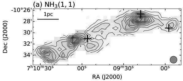
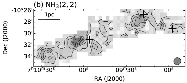
Figure 3: (a): Integrated intensity map of NH₃ (1,1). The lowest contour and contour steps are 0.2 K km s^-1 on the $T_{\mathrm{mb}}$ scale. Black crosses show the positions of the H₂O maser emission. (b): in (2,2). The lowest contour and contour steps are 0.1 K km s^-1. In each panel, the integrated velocity range is from 11.8 km s^-1 to 19.0 km s^-1. The beam size is indicated by the grey filled circle shown in the bottom right corner of each panel. (Color online)

Table 2: Coordinates and flux variations of H₂O masers.

ID	RA	Dec	1st observation	2nd observation	3rd observation
1	07:08:57.4	$-$10:29:10	6.25 Jy 03/12/2018	6.12 Jy 08/12/2018	2.05 Jy 16/02/2019
2	07:09:17.7	$-$10:26:40	1.73 Jy 14/02/2016
3	07:09:55.9	$-$10:31:03	0.85 Jy 08/05/2017	0.76 Jy 05/15/2017

Figure 2 shows the NH₃ (1,1) and (2,2) spectra at the position (a) – (c) of figure 1. In our observations, we can find five hyperfine lines consisting of one main line, two inner satellite lines, and two outer satellite lines in the (1,1) transition. In the (2,2) transitions only the main line was detected. Weak emission in the (3,3) main line ($T_{\mathrm{mb}}\simeq$ 0.11 K) was detected in the central position of IRAS 07077–1026 (position (b) shown in figure 1).

Figure 3-(a) shows the integrated intensity map of the NH₃ (1,1) main line. We found three bright regions in the NH₃ emission associated with PGCC G224.28–0.82, IRAS 07077–1026, and IRAS 07081–1028. The spatial distribution of the NH₃ emission is consistent with the Herschel dust continuum emission. This suggests that NH₃ emission lines are good tracers of dense molecular gas. The detailed analysis is described in subsection 3.5 and intensity correlations between the NH₃ (1,1) emission and the 250  dust emission are described in appendix B. Although the NH₃ beam size ($\sim$0.3 pc) is larger than the typical filament width ($\sim$0.1 pc), the spatial distribution of the NH₃ emission is expected to reflect the filamentary structure derived from the dust emission reported by Schisano et al. (2014) and Sewiło et al. (2019).

Figure 3-(b) shows the integrated intensity map of NH₃ (2,2). The NH₃ (2,2) line was detected in the region where (1,1) was strongly detected, and the strongest emission was detected in IRAS07077–1026. This implies that IRAS 07077–1026 has a higher temperature than the other regions.

We detected three new H₂O maser sources. Table 2 shows the position, flux densities and observation dates of each maser source. Table 2 shows the centres of the highest intensity pixels. While IRAS 07077–1026 was reported to be associated with a H₂O maser (e.g., Brand et al., 1994; Sunada et al., 2007), it was not detected in our observations. Detected maser spectra are shown in figure 15.

3.2 Ammonia line fitting

NH₃ (1,1) emission lines are split into 18 hyperfine components (HCs) by electric quadrupole interactions and magnetic spin-spin interactions (see Ho & Townes, 1983, for review). In cases where the velocity dispersion 0.2 km s^-1, only five blended hyperfine component groups (HCGs) can be observed. These HCGs are traditionally called the main line, two inner satellite lines, and two outer satellite lines, which consist of eight, three, and two HCs, respectively (see Rydbeck et al., 1977; Ho & Townes, 1983; Wang et al., 2020, for details).

Table 3: The parameters of hyperfine components for NH₃ (1,1).

HCG	HC number	F${}_{1}^{\prime}$ $\rightarrow$ F1	Relative Intensitya	fitting weight $w_{i}$b	Velocity offset [km s-1]
Outer satellite line 1	1	(1,0)	$\frac{2}{3}$	$\frac{2}{3}$	$-$19.55
	2	(1,0)	$\frac{1}{3}$	$\frac{1}{3}$	$-$19.41
Inner satellite line 1	3	(1,2)	$\frac{3}{5}$	$\frac{3}{5}$	$-$7.82
	4	(1,2)	$\frac{1}{15}$	$\frac{1}{15}$	$-$7.37
	5	(1,2)	$\frac{1}{3}$	$\frac{1}{3}$	$-$7.23
Main line	6	(2,2)	$\frac{1}{25}$	$\frac{1}{30}$	$-$0.25
	7	(1,1)	$\frac{5}{9}$	$\frac{5}{54}$	$-$0.21
	8	(2,2)	$\frac{14}{25}$	$\frac{7}{15}$	$-$0.13
	9	(1,1)	$\frac{1}{9}$	$\frac{1}{54}$	$-$0.07
	10	(2,2)	$\frac{9}{25}$	$\frac{3}{10}$	0.19
	11	(2,2)	$\frac{1}{25}$	$\frac{1}{30}$	0.31
	12	(1,1)	$\frac{1}{9}$	$\frac{1}{54}$	0.32
	13	(1,1)	$\frac{2}{9}$	$\frac{1}{27}$	0.46
Inner satellite line 2	14	(2,1)	$\frac{1}{15}$	$\frac{1}{15}$	7.35
	15	(2,1)	$\frac{3}{5}$	$\frac{3}{5}$	7.47
	16	(2,1)	$\frac{1}{3}$	$\frac{1}{3}$	7.89
Outer satellite line 2	17	(0,1)	$\frac{2}{3}$	$\frac{2}{3}$	19.32
	18	(0,1)	$\frac{1}{3}$	$\frac{1}{3}$	19.85

• The relative intensities are taken from table 15 of Mangum & Shirley (2015). The sum of the relative intensities of each of magnetic hyperfine splittings associating with each quadrupole hyperfine splitting are 1.

• The intensity ratio of (F${}_{1}^{\prime}$, F₁) = (1,1) to (2,2) is five to one; this ratio is used to correct for fitting weights of the main group.

To obtain the line width, we performed a relative intensity weighted Gaussian fit to all 18 HCs simultaneously at each observed position using the following equation (similar fitting procedure is described in Dhabal et al., 2019):

$$T_{\mathrm{mb}}(v)=\sum_{n=1}^{5}a_{n}\sum_{i}w_{i}\exp\left(-\frac{v-v_{\mathrm{los}}-\delta v_{i}}{2\sigma_{v}^{2}}\right),$$ (1)

where $a_{n}$ is the peak intensity of each HCG ($n$ = 1 to 5) in the case of well-blended HCGs are observed, $v_{\mathrm{los}}$ is the line-of-sight velocity of the main line, $\sigma_{v}$ is the velocity dispersion, $\delta v_{i}$ is the velocity offset of each HC from $v_{\mathrm{los}}$, and $w_{i}$ is the fitting weight of each HC ($i$ = 1 to 18 calculated from tables 11 and 15 of Mangum & Shirley, 2015). The $w_{1}$ to $w_{5}$ and $w_{14}$ to $w_{18}$ correspond to the relative hyperfine intensities of the magnetic hyperfine. NH₃ (1,1) main line contains two electric quadrupole hyperfine states of $\Delta F=0$. Therefore the $w_{6}$ to $w_{13}$ are calculated from the relative intensities of the magnetic hyperfine component and the electric quadrupole hyperfine component; the relative intensities of the magnetic hyperfine component are scaled by the relative intensities of the electric quadrupole hyperfine component and the sum of the $w_{6}$ to $w_{13}$ is 1. The $w_{i}$ and $\delta v$ are summarised in table 3. When the line width of the HCs is narrow, $a_{n}$ is not equal to the observed peak intensity of each HCG because individual HCs belonging to the same HCG do not overlap sufficiently, and the shape of the HCG does not follow a single Gaussian profile. Since the line width obtained from our observations are broad, we assume that $a_{n}$ is equal to the observed peak intensity of each HCG. We assume that all 18 hyperfine components have a same velocity dispersion, and each HC at the same HCG does not cause a hyperfine intensity anomaly.

We used a data cube with a velocity resolution smoothed to 0.38 km s^-1 to improve the signal-to-noise ratio (S/N) of the satellite lines. Line fitting was performed at positions where the main line detected more than 5$\sigma_{\mathrm{rms}}$. When $\sigma_{v}$ $>$ 1.0 km s^-1, NH₃ main line and inner satellite lines begin to overlap (Zhou et al., 2020). We applied $\sigma_{v}$ under the condition of 0.2 km s^-1 $<$ $\sigma_{v}$ $<$ 1.3 km s^-1 to account for noise effects in these fits, because no overlapping profile between main and inner satellite lines is observed.

Figures 4-(a) and (b) show maps of $v_{\mathrm{los}}$ and full width at half maximum (FWHM) line widths estimated by NH₃ (1,1) fittings. We can see a velocity gradient from northwest to southeast. The FWHM ranges from 0.6 km s^-1 to 3.1 km s^-1. The region of IRAS 07077–1026 shows that the line widths are broad.

In our observations, only the NH₃ (2,2) main line was detected. Although the main line consists of 12 HCs, single Gaussian fits were performed on the NH₃ (2,2) main line because the frequency of the 12 HCs in the main line HCG is too close to resolve them in our observations. In these fits, the line widths of the NH₃ (1,1) and (2,2) lines were assumed to be the same (see also Urquhart et al., 2011; Murase et al., 2022), and the fits were performed at positions where the NH₃ (2,2) main line was detected above 3$\sigma_{\mathrm{rms}}$. As with NH₃ (1,1), we used a data with a velocity resolution smoothed to 0.38 km s^-1.

The estimated NH₃ physical parameters were used in subsection 4. The estimated covariances from these fits were taken as errors of the estimated parameters.

3.3 Physical parameters from NH₃ lines

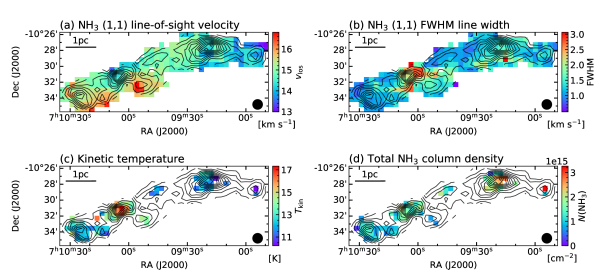
Figure 4: Spatial distributions of the physical parameters from NH₃ observations. (a): The line-of-sight velocity of the NH₃ (1,1) main line, (b): FWHM line width from the NH₃ (1,1) lines described in subsection 3.2, (c): Kinetic temperature, and (d): Total NH₃ column density. The contours and the black filled circle in the bottom right corner are the same as in figure 3-(a). (Color online)

We derived the optical depth, $\tau$, the kinetic temperature, $T_{\mathrm{kin}}$, and the column density, $N$(NH₃), from our NH₃ observations.

3.3.1 optical depth $\tau$

Under the local thermal equilibrium (LTE) conditions, the optical depth can be derived from the intensity ratio between the main and satellite lines of the NH₃ (1,1) emission (Ho & Townes, 1983). The optical depth can be derived from the following equation:

$$\frac{T_{\mathrm{mb}}(\mathrm{sate})}{T_{\mathrm{mb}}(\mathrm{main})}=\frac{1-\exp(-a\tau_{(1,1,\mathrm{m})})}{1-\exp(-\tau_{(1,1,\mathrm{m})})},$$ (2)

where $\tau_{\mathrm{(1,1,m)}}$ is the optical depth of the main line and $a$ is the relative intensity ratio of main to satellite lines, which is 0.27778 for the inner satellite lines or 0.22222 for the outer satellite lines (Mangum et al., 1992). In the optically thin case, the $a$ is the ratio of the total intensity of eight HCs forming the main line to the total intensity of two or three HCs forming the satellite line (see Mangum & Shirley, 2015). When the line width is relatively broad, the HCs are well-blended and each HCG has a single Gaussian profile, so the $a$ is approximately equal to the peak intensity ratio of the main line to the inner or outer satellite line. However, when the line width is narrow, the internal HCs are separated at each HCG and the $a$ does not match the peak intensity ratio between the main line and the inner or outer satellite line (see Zhou et al., 2020; Wang et al., 2020). Taking this effect into account, we derived the optical depth from the integrated intensity of the HCGs,

$$\frac{\int T_{\mathrm{mb}}(\mathrm{sate})\mathrm{d}v}{\int T_{\mathrm{mb}}(\mathrm{main})\mathrm{d}v}=\frac{1-\exp(-a\tau_{(1,1,\mathrm{m})})}{1-\exp(-\tau_{(1,1,\mathrm{m})})}.$$ (3)

To improve the S/N, we used the mean integrated intensity of two inner satellite lines for the satellite line intensity. The optical depth was calculated for pixels where the peak intensity of both inner satellite lines is greater than 5$\sigma_{\mathrm{rms}}$. The integrated velocity range for each HCG is approximately $v_{\mathrm{los}}$ $\pm$ 2.6$\sigma_{v}$. In this range, it is possible to integrate 99% of the radiation represented by the Gaussian profile.

3.3.2 The gas temperature

We used the following equation to derive the rotational temperature $T_{\mathrm{rot}}$ for pixels where the optical depth can be estimated and NH₃ (2,2) main lines were detected above 3$\sigma_{\mathrm{rms}}$,

$$T_{\mathrm{rot}}(2,2;1,1)=-41.2\Big{/}\ln\Big{(}\frac{-0.282}{\tau_{(1,1,\mathrm{m})}}\\ \times\ln\left[1-\frac{T_{\mathrm{mb}}(2,2,\mathrm{m})}{T_{\mathrm{mb}}(1,1,\mathrm{m})}\times[1-\exp(-\tau_{(1,1,\mathrm{m})})]\right]\Big{)}.$$ (4)

We converted the rotational temperature to the kinetic temperature using the following equation (Swift et al., 2005):

$$T_{\mathrm{rot}}=T_{\mathrm{kin}}\left\{1+\frac{T_{\mathrm{kin}}}{T_{0}}\ln[1+0.6\times\exp(-15.7/T_{\mathrm{kin}})]\right\}^{-1},$$ (5)

where $T_{0}$ is the energy difference between the (1,1) and (2,2) levels in Kelvin, which is 41.2 K. In the above equation, we used the value of a collision rate between NH₃ and hydrogen molecules reported by Danby et al. (1988).

Figure 4-(c) shows the spatial distribution of $T_{\mathrm{kin}}$. The range of $T_{\mathrm{kin}}$ is from 10.2 K to 17.3 K, and the mean value is 13.0 K. We found that the temperature around IRAS 07077–1026 is higher than the other regions.

3.3.3 The column density of NH₃

Under LTE conditions, NH₃ (1,1) column density, $N\mathrm{(1,1)}$, can be derived by the following equation (Mangum et al., 1992):

$$N(1,1)=6.60\times 10^{14}\frac{T_{\mathrm{rot}}}{\nu(1,1)}\tau_{(1,1,\mathrm{m})}V_{1/2},$$ (6)

where $\nu(1,1)$ is the rest frequency of NH₃ (1,1) in GHz, and $V_{1/2}$ is the FWHM of the NH₃ (1,1) main line in km s^-1. The total NH₃ column density, $N$(NH₃), is given by the following equation (Mangum et al., 1992):

$$N({\mathrm{NH_{3}}})=\\ N(1,1)\sum_{J}\sum_{K}\left[\frac{2g_{J}g_{I}g_{K}}{3}\exp\left(\frac{23.3-E(J,K)/k_{B}}{T_{\mathrm{rot}}}\right)\right],$$ (7)

where $g_{J}$ is the rotational degeneracy, $g_{I}$ is the nuclear spin degeneracy, and $g_{K}$ is the $K$–degeneracy. $E(J,K)/k_{\mathrm{B}}$ is the energy difference (in Kelvin) of each excited state from the ground state, using data from the JPL Molecular Spectroscopy catalogue (Pickett et al., 1998). The total NH₃ column density was calculated up to metastable states of ($J$,$K$) = (6,6), assuming that an ortho-to-para ratio is 1. The column density of NH₃ was calculated at positions where the rotational temperature could be derived as described above.

Figure 4-(d) shows that the spatial distribution of $N$(NH₃) does not vary significantly in most of the regions. This figure shows that $N$(NH₃) is distributed in the range of $2\times 10^{14}$ cm^-2 to $3.3\times 10^{15}$ cm^-2, and the mean value is $1.4\times 10^{15}$ cm^-2.

3.3.4 Error estimation

Estimating the error in observed physical parameters (i.e., optical depth, gas temperature, and column density) is important. In this paper, we evaluated the errors in these parameters by Monte Carlo method for each pixel (Murase et al., 2022, see for a similar algorithm). There are three following steps in error estimation, and we applied these in turn to equations (3)–(7):

1. consider the known error in the physical parameter as a standard deviation and generate a random number that follows a normal distribution;

2. substitute the best estimate of the known physical parameter + random number into the equation and derive the physical parameter with an unknown error;

3. repeat the above 10000 times and derive the standard deviation from the physical parameters obtained and consider it as the error inherent in the physical parameter.

The estimated errors of $T_{\mathrm{kin}}$ and $N$(NH₃) for NH₃ bright positions are summarised in table 4.

3.4 Physical parameters from CO lines

As a first step to figure out the physical conditions of the gas traced by the C¹⁸O emission, we derived the optical depth, $\tau$, the excitation temperature, $T_{\mathrm{ex}}$, and the column density, $N$(C¹⁸O), derived from the Mopra data. Before estimating these parameters, we performed single Gaussian fits to the C¹⁸O line. In this paper, we only used spectra with a S/N $\geq$ 3 to estimate the physical parameters.

Assuming that the ¹²CO emission is optically thick and the beam-filling factor is unity, the excitation temperature can be estimated by the following equation (e.g., Nagahama et al., 1998):

$$T_{\mathrm{ex}}=5.53\left[\ln\left(1+\frac{5.53}{T_{\mathrm{peak}}(^{12}\mathrm{CO})+0.819}\right)\right]^{-1},$$ (8)

where $T_{\mathrm{peak}}$(¹²CO) is the peak intensity of the ¹²CO emission. The $T_{\mathrm{ex}}$ ranges from 10.5 K to 17.8 K and the mean value is 13.9 K.

Assuming that the molecular clouds are under the LTE and have the same excitation temperature along the line-of-sight, and the beam-filling factor is unity, the optical depth of C¹⁸O can be obtained from the equation (Shimajiri et al., 2014):

$$\tau_{\mathrm{C^{18}O}}=-\ln\left(1-\frac{T_{\mathrm{peak}}(\mathrm{C^{18}O})}{5.27([\exp(5.27/T_{\mathrm{ex}})-1]^{-1}-0.1666)}\right),$$ (9)

where $T_{\mathrm{peak}}$(C¹⁸O) is the peak intensity of the C¹⁸O emission. The $\tau_{\mathrm{C^{18}O}}$ ranges from 0.04 to 0.44 and the mean value is 0.15.

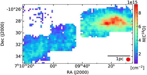
Figure 5: C¹⁸O column density map from the Mopra data. The red filled circle in the bottom right corner indicates the beam size of the Mopra data. (Color online)

The column density of C¹⁸O can be derived as follows (see Mangum & Shirley, 2015, for details):

$$\begin{split}N(\mathrm{C^{18}O})&=\frac{3h}{8\pi^{3}S\mu^{2}}\frac{Q_{\mathrm{rot}}}{g_{u}}\frac{\exp\left(\frac{E}{\kappa_{B}T_{\mathrm{ex}}}\right)}{\exp\left(\frac{h\nu}{\kappa_{B}T_{\mathrm{ex}}}\right)-1}\int\tau dv\\ &\simeq\frac{3h}{8\pi^{3}\mu^{2}}\frac{\exp\left(\frac{5.27}{T_{\mathrm{ex}}}\right)}{\exp\left(\frac{5.27}{T_{\mathrm{ex}}}\right)-1}\frac{Q_{\mathrm{rot}}}{J_{\nu}(T_{\mathrm{ex}})-J_{\nu}(T_{\mathrm{bg}})}\\ &\times\frac{\tau_{\mathrm{C^{18}O}}}{1-\exp(-\tau_{\mathrm{C^{18}O}})}\int T_{\mathrm{mb}}dv,\end{split}$$ (10)

where $S$ = $J/(2J+1)$ is the line strength, $\mu$ is the electric dipole moment, which is 0.11079 Debye for C¹⁸O, $g_{u}$ = $2J+1$ is the level degeneracy, $E/\kappa_{B}$ = 5.27 K is the energy difference of excited state from the ground state in Kelvin, $J_{\nu}(T)$ = $\frac{h\nu/k_{B}}{\exp(h\nu/(k_{B}T))-1}$ is the radiation temperature, and $T_{\mathrm{bg}}$ = 2.725 K is the temperature of cosmic microwave background radiation. The rest frequency of the C¹⁸O ($J$=1–0) emission line, $\nu$, is 109.782182 GHz. Also, the rotational partition function, $Q_{\mathrm{rot}}$, is given by,

$$Q_{\mathrm{rot}}=\sum_{J=0}^{\infty}(2J+1)\exp\left(-\frac{hB_{0}J(J+1)}{k_{B}T_{\mathrm{ex}}}\right),$$ (11)

where $B_{0}$ is the rigid rotor rotation constant, which was set to 54891.4 MHz. The electric dipole moment and rigid rotor rotation constant were taken from the JPL molecular spectroscopy catalogue (Pickett et al., 1998). The rotational partition function was calculated up to $J$=14. The errors of all physical parameters are derived by the Monte Carlo method.

Figure 5 shows the spatial distribution of the C¹⁸O column density. It shows that C¹⁸O molecular gases are concentrated at PGCC G224.28–0.82 and that there is no significant feature in the eastern part of the observed area. The $N$(C¹⁸O) ranges from 0.6 $\times$ 10¹⁵ cm^-2 to 9.2 $\times$ 10¹⁵ cm^-2 and the mean value of $N$(C¹⁸O) is 3.4 $\times$ 10¹⁵ cm^-2.

3.5 Deriving dust properties and spatial distributions

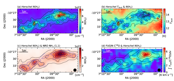
Figure 6: (a): The colour image and contours indicate the $N$(H₂) map obtained in subsection 3.5. The lowest contour and contour steps are 1.0 $\times$ 10²² cm^-2. (b): The dust temperature image obtained in subsection 3.5. The contours are the same as that shown in panel (a). (c): The colour image and black contours indicate the $N$(H₂) map derived from the Herschel data smoothed to be the same beam size as the NH₃ data. The lowest contour and contour steps are 1.0 $\times$ 10²² cm^-2. The blue dashed contours indicate NH₃ (1,1) integrated intensity, which are the same as in figure 1. (d): $N$(H₂) distributions (contours) superposed on the C¹⁸O integrated intensity map with the velocity range from 11.7 km s^-1 to 18.9 km s^-1 (colour image). The black contours are the same as the black contours in panel (c). In all panels, grey filled circle indicates the beam sizes of the Herschel data, and black filled circle indicates the 75 beam size. (Color online)

Using the $Herschel$ dust continuum data, we derived the dust temperature $T_{\mathrm{dust}}$ and the molecular hydrogen column density $N$(H₂), using the wavelengths, $\lambda$ from 160  to 500 . We made two data sets, the first is that all wavelength maps were smoothed to the beam size of 36.7 and regridded to 14, the second is that all wavelength maps were smoothed to the beam size of 75 and regridded to 37.5. Assuming that a molecular cloud has a single dust temperature along the line-of-sight and that the atomic hydrogen column density is negligibly low, SED fitting towards each pixel was performed by using the following equation:

$$I_{\nu}=B_{\nu}(T_{\mathrm{dust}})[1-e^{-\tau_{\nu}}],$$ (12)

where $I_{\nu}$ is the intensity at frequency $\nu$, $B_{\nu}$($T_{\mathrm{dust}}$) is the Planck blackbody function, $\tau_{\nu}=\kappa_{\nu}\Sigma$ is the dust optical depth, $\kappa_{\nu}$ is the dust opacity per unit mass (dust + gas), $\Sigma=\mu m_{\mathrm{H}}N$(H₂) is the surface gas density, $\mu$ is the mean molecular weight, and $m_{\mathrm{H}}$ is the atomic hydrogen mass. For consistency with Elia et al. (2013), we adopt $\kappa_{\nu}$ = $\kappa_{\lambda}$ = $0.1\times(\frac{\lambda}{250[\micron]})^{-\beta}$ [cm^-2 g^-1] assuming a gas-to-dust mass ratio of 100, a dust emissivity index $\beta$ of 2 (Hildebrand, 1983), and $\mu$ = 2.8 to take into account a relative helium abundance of 25% by mass (Kauffmann et al., 2008). Following Könyves et al. (2015), each data point of the SED fit was weighted by 1/$\sigma_{\mathrm{cal}}^{2}$, where $\sigma_{\mathrm{cal}}$ is the calibration error of surface brightness (20% at 160  and 10% at 250 , 350 , and 500 ). Its error estimate uses the covariance matrix.

Figure 6-(a) shows the spatial distribution of the $N(\rm{H_{2}})$. The high-column density is found around PGCC G224.28–0.82, IRAS 07077–1026, and IRAS 07081–1028. The $N$(H₂) ranges from 0.2 $\times$ 10²² to 8.3 $\times$ 10²² cm^-2.

Figure 6-(b) shows the spatial distribution of the $T_{\mathrm{dust}}$. We can see that the $T_{\mathrm{dust}}$ is higher at the edge of the cloud and lower at the centre. This temperature structure has generally been observed in the nearby molecular clouds and infrared dark clouds (e.g., Planck Collaboration et al., 2011; Sokolov et al., 2017). The dust temperature in the NH₃ observed area is 11 K – 14.5 K, which is almost the same as the distribution of the $T_{\mathrm{kin}}$ (figure 4-(c)).

Figure 6-(c) shows the map of the NH₃ (1,1) integrated intensity superposed on the $N$(H₂) derived from the dust continuum emission. In the NH₃ observed area, the NH₃ (1,1) integrated intensity and $N$(H₂) show good agreement with each other. On the other hand, the region between PGCC G224.28–0.82 and IRAS 07077–1026 has $N\mathrm{(H_{2})}>2.0\times 10^{22}$ cm^-2, while the NH₃ emission is very weak.

Figure 6-(d) shows the $N$(H₂) superposed on the map of the FUGIN C¹⁸O ($J$=1–0) integrated intensity. We can find no significant correlation between the C¹⁸O emission and the spatial distribution of $N$(H₂), except for PGCC G224.28–0.82. The C¹⁸O emissions were detected in the region between PGCC G224.28–0.82 and IRAS 07077–1026.

3.6 Identification of dense gas clumps with dendrogram

Table 4: Physical properties of the NH₃ clumps identified by the dendrogram.

clump ID	RA	Dec	$R$ [pc]	$T_{\mathrm{kin}}$ [K]	FWHM [km s-1]	$N$(NH3) [cm-2]	Mass [$\MO$]
1	07:08:55.9	$-$10:28:40.5	0.29	10.2 (0.6)	1.32 (0.03)	3.3 $\times$ 1015 (6 $\times$ 1014)	90 (10)
2	07:09:19.3	$-$10:27:42.3	0.32	11.6 (0.3)	1.43 (0.01)	2.1 $\times$ 1015 (2 $\times$ 1014)	290 (30)
3	07:09:51.5	$-$10:32:17.8	0.23	15 (1)	1.64 (0.05)	7 $\times$ 1014 (5 $\times$ 1014)	54 (7)
4	07:10:05.4	$-$10:31:28.2	0.26	16.1 (0.4)	2.18 (0.02)	1.6 $\times$ 1015 (2 $\times$ 1014)	110 (10)
5	07:10:12.7	$-$10:33:52.6	0.19	11.5 (0.7)	1.26 (0.02)	1.0 $\times$ 1015 (3 $\times$ 1014)	41 (6)
6	07:10:24.4	$-$10:33:47.6	0.39	12.1 (0.5)	1.16 (0.02)	1.4 $\times$ 1015 (2 $\times$ 1014)	220 (30)

• Notes: The physical parameters shown in this table are derived from the positions where the strongest NH₃ (1,1) integrated intensities were obtained for each clump. The errors are shown in parentheses.

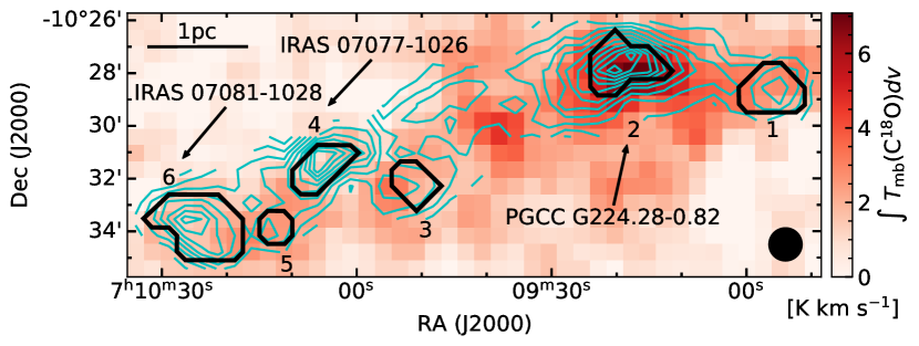
Figure 7: Integrated intensity map of NH₃ (1,1) in contours over the FUGIN C¹⁸O ($J$=1–0) integrated intensity image. The thick black polygons indicate the position and size of the clumps obtained from the dendrogram analysis in subsection 3.6. The contour steps and the black filled circle in the bottom right corner are the same as figure 3-(a). (Reprinted with permission from Handa et al. (2023). Copyright The Author(s), 2023 Published by Cambridge University Press on behalf of International Astronomical Union.) (Color online)

To identify the hierarchical structure of the molecular cloud, we performed a dendrogram analysis (Rosolowsky et al., 2008) on the NH₃ (1,1) main line data cube, which has a velocity resolution of 0.19 km s^-1 and a typical rms noise level of 0.035 K. This analysis uses the following three parameters: min_value, min_delta, and min_npix, where min_value is a parameter to distinguish between structure and noise, min_delta is the threshold to separate multiple structures, and min_npix is the minimum number of pixels to identify a structure, respectively. In this paper, we used the input with the min_value = 3$\sigma$, min_delta = 3$\sigma$, where $\sigma=$ 0.035 K is the rms noise, and min_npix = 4 pixels, which is a minimum integer number of pixels larger than the beam size. In addition, we have added the condition that the peak intensity of the structure is greater than 7$\sigma$ and that the structure has a spread of two channels or more in the velocity axis. We refer to a ”leaf” as a clump in the dendrogram output.

Figure 7 shows the results of the dendrogram analysis. The six NH₃ clumps were identified. We gave an identification number from west to east for each clump. The centre of PGCC G224.28–0.82 corresponds to the clump 2, IRAS 07077–1026 and IRAS 07081–1028 correspond to the clumps 4 and 6, respectively. We adopted $R=\sqrt{A/\pi}$ as the clump radius, where $A$ is the total area on the sky in a clump. The clump radius ranges from 0.19 pc to 0.39 pc. We estimated the mass of each clump using Mass = $\mu m_{\mathrm{H}}A_{\mathrm{pixel}}\sum_{i}N_{i}(\mathrm{H_{2}})$, where $A_{\mathrm{pixel}}$ is the surface area of the pixel and the $N_{i}$(H₂) is the $N$(H₂) of each pixel belonging to each clump. This calculation uses the $N$(H₂) data derived in subsection 3.5, which has a resolution of 75. The clump mass ranges from 41 $\MO$ to 290 $\MO$. Only the clump 2 is massive enough to fulfil the empirical threshold for high-mass star formation, $M(r)>870\ \MO$ (radius/pc)^1.33 (Kauffmann & Pillai, 2010). The physical parameters of the clumps are summarised in table 4.

4 discussion

4.1 Comparison of the NH₃ and C¹⁸O

Figure 7 shows the integrated intensity of the NH₃ (1,1) main line superposed on the integrated intensity map of the FUGIN C¹⁸O. The spatial distributions of the two emission lines appear to be consistent in most of our observed area, but in particular in the clumps 4 and 6 (IRAS 07077–1026 and IRAS 07081–1028) the distributions are different. The spatial range of the distributional discrepancy is about $\sim$1 pc. To investigate this more quantitatively, we made an integrated intensity correlation plot (figure 8). In this plot, we used the pixels contained in the clumps identified by the dendrogram analysis.

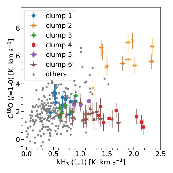
Figure 8: NH₃ (1,1) – C¹⁸O ($J$=1–0) integrated intensity correlation plot of the each clump and the other positions. (Reprinted with permission from Handa et al. (2023). Copyright The Author(s), 2023 Published by Cambridge University Press on behalf of International Astronomical Union.) (Color online)

We can find two features in figure 8: a positive correlation in the clump 2, with a correlation coefficient of $r=0.42$, while negative correlations are found in the clumps 4 and 6, with $r$ of $-$0.56 and $-$0.41, respectively. Since the critical density of NH₃ (1,1) and C¹⁸O ($J$=1–0) is almost the same, both emission lines are expected to be emitted from the same region in the molecular cloud. Therefore, our results suggest that the C¹⁸O emission line intensity is suppressed compared to the NH₃ emission in the clumps 4 and 6.

The distributional discrepancy between the integrated intensity of the C¹⁸O ($J$=1–0) and the $N$(H₂) or the integrated intensity of the NH₃ (1,1) could have several causes; including CO depletion, photodissociation where the molecules are destroyed by UV radiation, and high-density gas dissipation. These possibilities will be discussed in the next subsection.

4.2 Cause of weak C¹⁸O emission in dense clump

In subsection 4.1, we showed two regions where the C¹⁸O emission line is almost undetectable despite high H₂ column density. This phenomenon in the clump 4 was also reported by Olmi et al. (2016). They described two possible causes for this phenomenon: CO depletion and differences in the temperature dependence of CO and dust emissions. It has also been slightly discussed by Sewiło et al. (2019), together with the detection of the H₂O maser, the high density gas has been interpreted as a decrease in the clump 4. However, this phenomenon is hardly discussed in the previous studies and the reason for this discrepancy is not identified. In this subsection we will discuss the cause of this discrepancy, and the clump 4 will be treated as the main subject of discussion unless otherwise stated.

Sewiło et al. (2019) suggested that the gas in the the clump 4 may be decreasing by dissipation. In general, if the gas density is sufficiently lower than the critical density, the molecular emission line cannot be detected. However, $\rm{N_{2}H^{+}}$ ($J$=1–0) emission line was detected in this region (Tatematsu et al., 2017). The critical density of $\rm{N_{2}H^{+}}$ ($J$=1–0) is $4.1\times 10^{4}$ cm^-3 at $T$ = 20 K (Shirley, 2015), which is an order of magnitude higher than that of C¹⁸O ($J$=1–0). It is therefore unlikely that the cause of the discrepancy is a decrease in the gas density. Furthermore, the luminosity-mass ratio, $L_{\mathrm{bol}}/\MO$, of three dust clumps associated with the region within a 1.$\arcmin$5 radius of the central position of the clump 4 was less than 1.0 (Elia et al., 2013). Sources with $L_{\mathrm{bol}}/\MO$ $<$ 1 contain either low-mass protostars or early-stage intermediate-mass/high-mass protostars (Molinari et al., 2016). Also, the H₂O maser does not reflect a well-defined evolutionary stage of the host YSOs (Titmarsh et al., 2016). Therefore, the cause of the discrepancy is unlikely to be dense gas dispersion.

We considered that C¹⁸O molecules are likely to be destroyed by photodissociation (e.g., Glassgold et al., 1985). Photodissociation is a phenomenon in which a molecule dissociates when it collides with a high-energy photon. Photodissociation is often detected near the boundary surface between Hii regions and molecular clouds. The two IRAS sources reported the candidate for an ultra-compact (UC) Hii region (Bronfman et al., 1996). However, two IRAS sources are not listed in the catalogue of the Hii region using the Wide-Field Infrared Survey Explorer (Anderson et al., 2014). Furthermore, in and around two IRAS sources, there are no Red MSX Source objects, which are candidates for high-mass young stellar objects and Compact or UC Hii regions. Therefore, the clumps 2 and 4 are unlikely to contain a Hii region. In addition, the dissociation energies of CO and NH₃ are 11.092 eV and 4.3 eV, respectively (Däppen, 2002). It is natural to assume that if a photodissociation region is formed, NH₃ molecules will be destroyed before C¹⁸O molecules, making NH₃ lines undetectable. Furthermore, it is common that for dust clumps associated with Hii region to have $L_{\mathrm{bol}}/\MO 40$ (Giannetti et al., 2017). Considering that dust clumps associated with the clumps 4 and 6 have $L_{\mathrm{bol}}/\MO$ $<$ 2, the cause of the discrepancy is unlikely to be the destruction of C¹⁸O molecules by photodissociation.

We believe that CO depletion is the most likely cause of the discrepancy. Both the kinetic temperature and the dust temperature in and around the clumps 4 and 6 are lower than 20 K, which is temperature criterion for CO depletion. N₂H⁺ which detected in the clump 4 immediately reacts with CO in the gas-phase to form HCO⁺ (e.g., Jørgensen et al., 2004). In other words, the detection of N₂H⁺ implicitly indicates that CO depletion is occurring at least in the centre of the region. It is therefore suggested that the C¹⁸O line cannot detect high density gas in the clump 4 due to the CO depletion.

Based on this idea, some questions remain as to why CO depletion occurs in the clump 4. First, CO depletion is a temperature dependent phenomenon. It is somewhat unnatural that CO depletion occurs in the clump 4, even though both the dust temperature and the kinetic temperature are higher than the ambient temperature. However, in the clump 4, the dust temperature and the kinetic temperature are 14 K and 17 K, respectively, and CO depletion can occur under these conditions (e.g., Pillai et al., 2007; Fontani et al., 2012; Feng et al., 2020). It is therefore not surprising that CO depletion occurs even at slightly higher temperatures than in the surrounding region. Second, a SiO emission line is also detected in IRAS 07077–1026 (Harju et al., 1998). This suggests that the outflow shock associated with a protostar destroys the icy mantle of dust grains. However, the outflow shock is highly directional and is unlikely to affect the entire clump. In fact, outflow and CO depletion have been found to occur simultaneously (Tobin et al., 2013; Feng et al., 2016a, b). Therefore, this idea is consistent with previous studies.

It is unclear whether CO depletion occurs everywhere within the clump; Olmi et al. (2023) reported that an ALMA observation of dust clump within the clump 4, named HG2825, has detected strong C¹⁸O emission. Ge et al. (2020) also proposed that there are multiple cores overlapping towards the line-of-sight in this region, forming a complex distribution of different molecular species. High-resolution CO observations over the entire clump are necessary to understand the inner structure.

The clump 6 shows similar features to the clump 4 on the integrated intensity correlation plot of the NH₃ (1,1) and C¹⁸O ($J$=1–0) (figure 8). However, due to the lack of N₂H⁺ observations, it is unclear whether CO depletion occurs in the clump 6. Further observations are needed to verify this.

Our results suggest that the presence of pc-scale CO depletion can be detected by comparing the integrated intensity of NH₃ and C¹⁸O, such as in low-mass star-forming regions (Willacy et al., 1998). Since molecular clouds are concentrated in the Galactic plane and crowded towards the line of sight, it is difficult to compare the distributions of the dust continuum and C¹⁸O line emission, and to accurately estimate the properties of depleted regions. Molecular emission lines can be separated using the velocity field information, and the intensities of the emission lines can be easily compared. In addition, the NH₃ line provides many physical parameters, such as gas temperature and column density (see subsection 4). Comparing the intensity distributions of NH₃ and C¹⁸O lines will allow us to identify many candidates for pc-scale CO depletion in the Galactic plane and to make statistical arguments about the physical conditions of the pc-scale CO depletion.

4.3 C¹⁸O depletion factor

It is a common practice to use the depletion factor, $f_{\mathrm{D}}$ (e.g., Caselli et al., 1999), in order to evaluate the degree of CO depletion. The definition of $f_{\mathrm{D}}$ is as follows,

$$f_{\mathrm{D}}=\frac{X^{\mathrm{E}}(\mathrm{C^{18}O})}{X^{\mathrm{O}}(\mathrm{C^{18}O})},$$ (13)

where $X^{\mathrm{E}}$(C¹⁸O) is the ”expected” (i.e., canonical) relative abundance of C¹⁸O molecules to molecular hydrogen and $X^{\mathrm{O}}$(C¹⁸O) is the observed one. The C¹⁸O abundance of the solar neighbourhood or the C¹⁸O abundance predicted by the galactocentric distance are frequently used as the $X^{\mathrm{E}}$(C¹⁸O).

The depletion factor obtained from equation (13) varies by a factor of several, depending on assumptions such as dust opacity. When discussing only a single molecular cloud, focusing on changes in the depletion factor within a cloud would reduce the impact of the underlying assumptions. Therefore, we defined the ”relative” depletion factor at the same molecular cloud, $f_{\mathrm{D}}^{\mathrm{R}}$:

$$f_{\mathrm{D}}^{\mathrm{R}}=\frac{X^{\mathrm{M}}(\mathrm{C^{18}O})}{X^{\mathrm{O}}(\mathrm{C^{18}O})},$$ (14)

where $X^{\mathrm{M}}$(C¹⁸O) is the maximum $X^{\mathrm{O}}$(C¹⁸O) in the observed region. We calculated C¹⁸O relative abundance, $X\rm{(C^{18}O)}$, and the $X\rm{(C^{18}O)}$ in the NH₃ observed area ranges from $4\times 10^{-8}$ to $3.7\times 10^{-7}$. To improve reliability, the value of $X^{\mathrm{M}}$(C¹⁸O) is determined from observed pixels that represent more than 15 times the error of $N$(C¹⁸O), and we adopt $2.6\times 10^{-7}$.

Figure 9: The spatial distribution of the relative depletion factor, $f_{\mathrm{D}}^{\mathrm{R}}$. The contours are the same as in figure 6-(a). The red filled circle in the bottom right corner indicates the beam size of the Mopra data. (Color online)

Figure 9 shows the spatial distribution of $f_{\mathrm{D}}^{\mathrm{R}}$ derived from the Mopra data. The $f_{\mathrm{D}}^{\mathrm{R}}$ is about 3.5 to 6.5 in and around the clump 4, and about 1.5 to 3.5 in and around the clump 2. The freeze-out rate of $\mathrm{C^{18}O}$ is about 2 to 4 times higher in the clump 4 than in the clump 2.

We found the pc-scale CO depletion in the clump 4 (figure 9). Feng et al. (2020) have reported that 70  dark clumps with pc-scale CO depletion have a depletion factor about 2 to 4 times larger than 70  bright clumps without CO depletion at the same IRDCs. The trend of CO depletion observed in the clump 4 is similar to that of previous studies. While these 70  dark clumps fulfil the empirical threshold for high-mass star formation (Kauffmann & Pillai, 2010), the clump 4 is a relatively low-mass clump and is below the empirical threshold. A relatively low-mass clump that cannot form high-mass stars was found to have the same trend of pc-scale CO depletion as high-mass clumps.

4.4 The condition of weak CO depletion in the centre of PGCC G224.28–0.82

From figure 9, we can see that the CO depletion state is different within the observed region. The star-forming clumps located in the observed region can be regarded as having substantially the same external physical conditions and initial conditions for the dense gas formation. It would be important to study the differences in the CO depletion state; the differences in the CO depletion state of the clumps may affect the chemical diversity of the pre/proto-stellar core, since the possibility has been suggested that prestellar cores grow by mass accretion from the surroundings during the protostar formation process (Takemura et al., 2021). In this subsection, we focus on the differences in physical properties between the clump 2 and clump 4.

To investigate the difference in CO depletion state, we compared the temperature and volume density of these clumps. In the clump 2, $T_{\mathrm{dust}}$ and $T_{\mathrm{kin}}$ are both approximately 12 K, and the mean gas density, calculated assuming the clump is a symmetric sphere, is estimated to be $4\times 10^{4}$ cm^-3. In the clump 4, $T_{\mathrm{dust}}$ $\simeq$ 14 K, $T_{\mathrm{kin}}$ $\simeq$ 16 K, and the mean gas density is estimated to be 3 $\times$ 10⁴ cm^-3.

These estimates fulfil the conditions for the occurrence of CO depletion. In other words, if CO depletion has occurred in the clump 4, it is natural that CO depletion should also occur in the clump 2. The clump 2 fulfils the empirical threshold for high-mass star formation, and intuitively, clump 2 is more likely to cause pc-scale CO depletion than clump 4. Since the gas and dust temperatures at the clump 4 are higher than at the clump 2, and the clumps 2 and 4 also have similar densities, this difference is not caused by temperature and density. In the clump 2, there is only weak CO depletion. Therefore the C¹⁸O ($J$=1–0) emission can trace the dense gas. This implies that what determines the conditions under which C¹⁸O ($J$=1–0) emission line can and cannot trace dense gas is unclear.

This phenomenon is possibly caused by non-thermal desorption such as photodesorption, chemical sputtering. Molecules frozen onto dust grains may have been released into the gas phase by photodesorption at the clump 2. Figure 10 shows the spatial distribution of $f_{\mathrm{D}}^{\mathrm{R}}$ and the locations of the protostar candidates reported by Sewiło et al. (2019), classified by bolometric luminosity and evolutionary stages of YSO. As this figure shows, there are three protostars with bolometric luminosity above 100 $\LO$ in the vicinity of only the clump 2. These protostars have only a disk and with no envelope, and can affect the surrounding environment. Furthermore, even protostars deeply embedded in molecular clouds may be able to influence the surrounding environment, if molecular clouds have clumpy structures as proposed by previous studies (e.g., Spaans, 1996; Kramer et al., 2008; Shimajiri et al., 2014); as a result, molecules frozen onto dust grains are released into the gas phase by photodesorption.

However, photodesorption is well known to occur in the cold outer regions of proto-planetary disks (e.g., Öberg et al., 2015) as well as in the centre of the pre-stellar core (e.g., Caselli et al., 2012), but it is not known in a cold clump at the pc scale. Therefore, our proposal needs further verification. In order to study the effects of photodesorption by radiation from protostars on the surrounding environment, observations of molecular species such as H₂O, whose abundance increases with photodesorption, are essential.

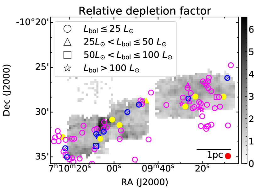
Figure 10: The locations of the protostar candidates (plots) superposed on the relative depletion factor map (colour image). Magenta open, blue hatched, and yellow filled markers indicate “disk-only” sources, “envelope and disk” sources, and “envelope-only” sources, respectively. The red filled circle in the bottom right corner indicates the beam size of the Mopra data. (Color online)

5 Conclusions

We carried out mapping observations towards the star-forming region, which is the vicinity of ($\alpha_{\mathrm{J2000}},\delta_{\mathrm{J2000}}$) = (07:09:20.30, $-$10:27:55) associated with CMa OB1 in the NH₃ (1,1), (2,2), (3,3), and H₂O maser emission lines using the Nobeyama 45 m radio telescope. Our results are summarised as follows:

1. Our observations revealed physical parameters of the observed region such as $T_{\mathrm{kin}}$ and $N$(NH₃). The $T_{\mathrm{kin}}$ ranges from 10.2 K to 17.3 K, with IRAS 07077–1026 having a higher temperature by about 3 K higher than the other regions. The total column density of NH₃ does not vary significantly in most of the regions. The mean value is $N$(NH₃) = $1.4\times 10^{15}$ cm^-2.

2. We carried out a dendrogram analysis using NH₃ (1,1) main line data and identified six clumps. The centre of PGCC G224.28–0.82 corresponds to the clump 2, IRAS 07077–1026 and IRAS 07081–1028 correspond to the clumps 4 and 6, respectively. The clump radius ranges from 0.19 pc to 0.39 pc and clump mass ranges from 41 $\MO$ to 290 $\MO$. Only the clump 2 fulfils the empirical threshold for high-mass star formation.

3. By comparing the spatial distributions of the NH₃ (1,1) integrated intensity and the C¹⁸O ($J$=1–0) integrated intensity, we found pc-scale intensity anti-correlations in the clump 4 and clump 6. Moreover, the comparison of these integrated intensity distributions with the distribution of $N$(H₂) obtained from the dust shows that the NH₃ molecular emission lines reflect the distribution of $N$(H₂) well, even at the pc scale. On the contrary, the intensity distribution of the C¹⁸O emission lines does not correlate well with the distribution of $N$(H₂), and some high-density regions cannot be detected at the pc scale. By examining the dissipation of the high-density gas, photodissociation, and CO depletion, we suggest that the reason why C¹⁸O ($J$=1–0) does not trace $N$(H₂) is due to CO depletion in the clump 4. A comparison of the intensity distributions of the NH₃ and C¹⁸O lines will allow us to identify candidates for pc-scale CO depletion.

4. We calculated the relative depletion factor, $f_{\mathrm{D}}^{\mathrm{R}}$, and compared the $f_{\mathrm{D}}^{\mathrm{R}}$ of high H₂ column density regions, the clump 2 and clump 4. There are differences in $f_{\mathrm{D}}^{\mathrm{R}}$ by a factor of about 2 to 4. This is comparable to the difference in depletion factor between the 70  dark clump and the 70  bright clump in the same molecular cloud reported by Feng et al. (2020).

5. We discussed why there is weak CO depletion in the clump 2. The difference in temperature and gas density does not explain this phenomenon well and the conditional differences that C¹⁸O ($J$=1–0) can and cannot trace dense gas are unclear. Non-thermal desorption such as photodesorption may play a key role in changing the CO depletion state.

The 45 m radio telescope is operated by the Nobeyama Radio Observatory, a branch of the National Astronomical Observatory of Japan. This publication makes use of data from FUGIN, FOREST Unbiased Galactic plane Imaging survey with the Nobeyama 45 m telescope, a legacy project in the Nobeyama 45 m radio telescope. Figure 7 and Figure 8 are reprinted with permissoin from Handa et al., Parsec scale CO depletion in KAGONMA 71, or a star-forming filament in CMa OB1, Proceedings of the International Astronomical Union, 17(S373), 31-34, 2023. (Copyright The Author(s), 2023 Published by Cambridge University Press on behalf of International Astronomical Union.) This research made use of aplpy, an open-source plotting package for Python (Robitaille & Bressert, 2012), astropy, a community-developed core Python package for Astronomy (Astropy Collaboration et al., 2013, 2018), matplotlib, a Python package for visualization (Hunter, 2007), numpy, a Python package for scientific computing (Harris et al., 2020), pandas a Python package for statistical analysis, data manipulations and processing (Wes McKinney, 2010), scipy, a Python package for fundamental algorithms for scientific computing (Virtanen et al., 2020), and Overleaf, a collaborative tool. We would like to thank the Nobeyama Radio Observatory staff members (NRO) for their assistance and observation support. We also thank the students of Kagoshima University for their support in the observations.

Appendix A Intensity differences of ¹²CO

Figure 11 shows the intensity correlation between the Mopra ¹²CO and the FUGIN ¹²CO. The FUGIN ¹²CO data was smoothed to the beam size of the Mopra data and regridded to the grid size of the Mopra data. The Mopra ¹²CO data was smoothed to the velocity resolution of the FUGIN data and was interpolated onto the FUGIN data grid. The resulting rms noise of the FUGIN ¹²CO is 1.2 K and that of the Mopra ¹²CO is 0.30 K. We plot the data for 11 channels ranging from 11.7 km s^-1 to 18.2 km s^-1. They fit well with a linear function of $T_{\mathrm{mb}}$(FUGIN ¹²CO) = 0.764 $\times$ $T_{\mathrm{mb}}$(Mopra ¹²CO) + 0.127; the red line overlaid on the data shows the best-fit linear function. The intensity of the Mopra ¹²CO data is systematically 1/0.764 $\simeq$ 1.3 times greater than the intensity of the FUGIN ¹²CO data. We obtained the result $T_{\mathrm{mb}}$(FUGIN C¹⁸O) = 0.973 $\times$ $T_{\mathrm{mb}}$(Mopra C¹⁸O) $-$ 0.038 from the similar analysis using the C¹⁸O data. There is no significant difference in intensity between the FUGIN C¹⁸O and the Mopra C¹⁸O. It is not known whether the problem is in the FUGIN ¹²CO data or the Mopra ¹²CO data and what the cause might be. The following paragraph describes the effect on the physical parameters, in the case of the intensity of the Mopra ¹²CO data was 30% higher than in reality.

We re-calculated $T_{\mathrm{ex}}$, $\tau_{\mathrm{C^{18}O}}$, $N$(C¹⁸O), $X$(C¹⁸O), and $f_{\mathrm{D}}^{\mathrm{R}}$. The intensity of the Mopra ¹²CO was scaled by a factor of 0.764 and the following physical parameters were derived without changing other conditions. The $T_{\mathrm{ex}}$ changes by a factor of 0.81 to 0.84. The $\tau_{\mathrm{C^{18}O}}$ changes by a factor of 1.3 to 1.4. The $N$(C¹⁸O) and the $X$(C¹⁸O) change by a factor of 0.91 to 1.0. The $f_{\mathrm{D}}^{\mathrm{R}}$ changes by a factor of 0.94 to 1.0. Figure 12 shows the re-calculated $N$(C¹⁸O) and figure 13 shows the re-calculated $f_{\mathrm{D}}^{\mathrm{R}}$. Both the values and the spatial distributions are not significantly different from those before the re-calculation.

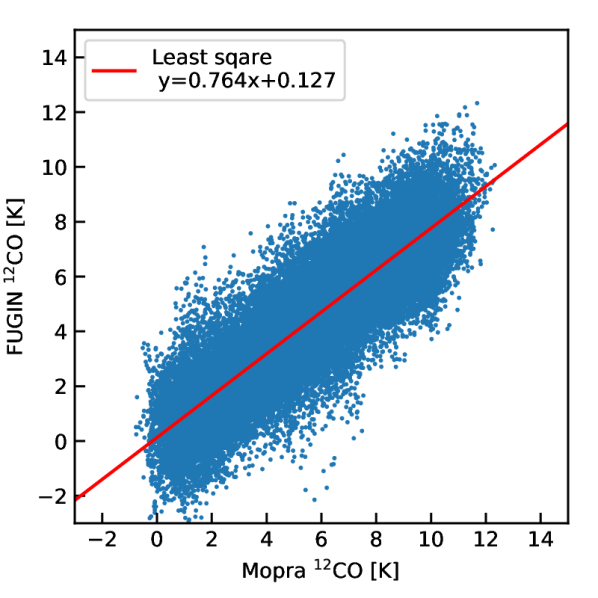
Figure 11: Intensity correlation between the Mopra ¹²CO and the FUGIN ¹²CO. The data from the 11 channels in the range from 11.7 km s^-1 to 18.2 km s^-1 are plotted. The red line shows the best-fit linear function determined by a least-squares method. (Color online)

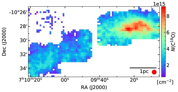
Figure 12: Same as figure 5 but for the re-calculated C¹⁸O column density map derived from the Mopra ¹²CO data with the intensity scaled by a factor of 0.764. (Color online)

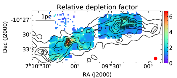
Figure 13: Same as figure 9 but for the re-calculated relative depletion factor derived from the re-calculated C¹⁸O column density. (Color online)

Appendix B Correlations between NH₃ (1,1) and Dust emission

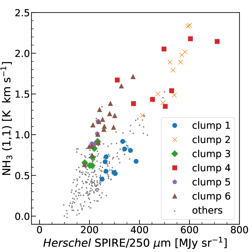
Figure 14: The correlation diagram between the NH₃ integrated intensity and the dust emission intensity at 250 . The dust emission data was smoothed to a beam size of 75. All points are colour coded for each clump and non-clump. (Color online)

Figure 14 is the correlation plot between the NH₃ (1,1) integrated intensity and the dust emission intensity at 250 . The correlation coefficient between these two data across all pixels is 0.83. There is a clear positive correlation and the same trend regardless of the strength of the two emissions.

Appendix C H₂O maser spectrum

Figure 15 shows the spectra of the H₂O masers listed in table 2.

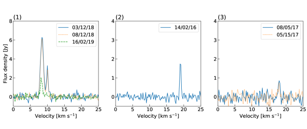
Figure 15: The H₂O maser emission from our observations. The detected dates and positions are listed in table 2. (Color online)

References

- Anderson et al. (2014) Anderson, L. D., Bania, T. M., Balser, D. S., Cunningham, V., Wenger, T. V., Johnstone, B. M., & Armentrout, W. P. 2014, ApJS, 212, 1
- Astropy Collaboration et al. (2013) Astropy Collaboration, et al. 2013, A&A, 558, A33
- Astropy Collaboration et al. (2018) Astropy Collaboration, et al. 2018, AJ, 156, 123
- Bergin & Tafalla (2007) Bergin, E. A., & Tafalla, M. 2007, ARA&A, 45, 339
- Brand et al. (1994) Brand, J., et al. 1994, A&AS, 103, 541
- Bronfman et al. (1996) Bronfman, L., Nyman, L. A., & May, J. 1996, A&AS, 115, 81
- Caselli et al. (1999) Caselli, P., Walmsley, C. M., Tafalla, M., Dore, L., & Myers, P. C. 1999, ApJ, 523, L165
- Caselli et al. (2012) Caselli, P., et al. 2012, ApJ, 759, L37
- Clariá (1974) Clariá, J. J. 1974, A&A, 37, 229
- Crapsi et al. (2007) Crapsi, A., Caselli, P., Walmsley, M. C., & Tafalla, M. 2007, A&A, 470, 221
- Dame et al. (2001) Dame, T. M., Hartmann, D., & Thaddeus, P. 2001, ApJ, 547, 792
- Danby et al. (1988) Danby, G., Flower, D. R., Valiron, P., Schilke, P., & Walmsley, C. M. 1988, MNRAS, 235
- Däppen (2002) Däppen, W. 2002, in Allen’s Astrophysical Quantities, ed. A. N. Cox (New York: Springer), 27–51
- Dhabal et al. (2019) Dhabal, A., Mundy, L. G., Chen, C. -y., Teuben, P., & Storm, S. 2019, ApJ, 876, 108
- Elia et al. (2013) Elia, D., et al. 2013, ApJ, 772, 45
- Feng et al. (2016a) Feng, S., Beuther, H., Zhang, Q., Henning, T., Linz, H., Ragan, S., & Smith, R. 2016a, A&A, 592, A21
- Feng et al. (2016b) Feng, S., Beuther, H., Zhang, Q., Liu, H. B., Zhang, Z., Wang, K., & Qiu, K. 2016b, ApJ, 828, 100
- Feng et al. (2020) Feng, S., et al. 2020, ApJ, 901, 145
- Fischer et al. (2016) Fischer, W. J., Padgett, D. L., Stapelfeldt, K. L., & Sewiło, M. 2016, ApJ, 827, 96
- Fontani et al. (2012) Fontani, F., Giannetti, A., Beltrán, M. T., Dodson, R., Rioja, M., Brand, J., Caselli, P., & Cesaroni, R. 2012, MNRAS, 423, 2342
- Frerking et al. (1982) Frerking, M. A., Langer, W. D., & Wilson, R. W. 1982, ApJ, 262, 590
- Ge et al. (2020) Ge, J. X., et al. 2020, ApJ, 891, 36
- Giannetti et al. (2017) Giannetti, A., Leurini, S., Wyrowski, F., Urquhart, J., Csengeri, T., Menten, K. M., König, C., & Güsten, R. 2017, A&A, 603, A33
- Glassgold et al. (1985) Glassgold, A. E., Huggins, P. J., & Langer, W. D. 1985, ApJ, 290, 615
- Gong et al. (2018) Gong, Y., Li, G. X., Mao, R. Q., Henkel, C., Menten, K. M., Fang, M., Wang, M., & Sun, J. X. 2018, A&A, 620, A62
- Griffin et al. (2010) Griffin, M. J., et al. 2010, A&A, 518, L3
- Handa et al. (2023) Handa, T., et al. 2023, IAU Symposium, 373, 31
- Harju et al. (1998) Harju, J., Lehtinen, K., Booth, R. S., & Zinchenko, I. 1998, A&AS, 132, 211
- Harris et al. (2020) Harris, C. R., et al. 2020, Nature, 585, 357
- Hernandez et al. (2011) Hernandez, A. K., Tan, J. C., Caselli, P., Butler, M. J., Jiménez-Serra, I., Fontani, F., & Barnes, P. 2011, ApJ, 738, 11
- Hildebrand (1983) Hildebrand, R. H. 1983, QJRAS, 24, 267
- Ho & Townes (1983) Ho, P. T. P., & Townes, C. H. 1983, ARA&A, 21, 239
- Hunter (2007) Hunter, J. D. 2007, Computing in Science & Engineering, 9, 90
- Jiménez-Serra et al. (2014) Jiménez-Serra, I., Caselli, P., Fontani, F., Tan, J. C., Henshaw, J. D., Kainulainen, J., & Hernandez, A. K. 2014, MNRAS, 439, 1996
- Jørgensen et al. (2004) Jørgensen, J. K., Schöier, F. L., & van Dishoeck, E. F. 2004, A&A, 416, 603
- Kaltcheva & Hilditch (2000) Kaltcheva, N. T., & Hilditch, R. W. 2000, MNRAS, 312, 753
- Kauffmann et al. (2008) Kauffmann, J., Bertoldi, F., Bourke, T. L., Evans, N. J., I., & Lee, C. W. 2008, A&A, 487, 993
- Kauffmann & Pillai (2010) Kauffmann, J., & Pillai, T. 2010, ApJ, 723, L7
- Kim et al. (2004) Kim, B. G., Kawamura, A., & Fukui, Y. 2004, PASJ, 56, 313
- Kohno et al. (2022) Kohno, M., et al. 2022, PASJ, 74, 545
- Kohno et al. (2023) Kohno, M., et al. 2023, PASJ, 75, 397
- Könyves et al. (2015) Könyves, V., et al. 2015, A&A, 584, A91
- Kramer et al. (1999) Kramer, C., Alves, J., Lada, C. J., Lada, E. A., Sievers, A., Ungerechts, H., & Walmsley, C. M. 1999, A&A, 342, 257
- Kramer et al. (2008) Kramer, C., et al. 2008, A&A, 477, 547
- Kuno et al. (2011) Kuno, N., et al. 2011, in 2011 XXXth URSI General Assembly and Scientific Symposium, 1–4
- Ladd et al. (2005) Ladd, N., Purcell, C., Wong, T., & Robertson, S. 2005, PASA, 22, 62
- Lewis et al. (2021) Lewis, J. A., Lada, C. J., Bieging, J., Kazarians, A., Alves, J., & Lombardi, M. 2021, ApJ, 908, 76
- Lin et al. (2021) Lin, Z., Sun, Y., Xu, Y., Yang, J., & Li, Y. 2021, ApJS, 252, 20
- Lombardi et al. (2014) Lombardi, M., Bouy, H., Alves, J., & Lada, C. J. 2014, A&A, 566, A45
- Mangum & Shirley (2015) Mangum, J. G., & Shirley, Y. L. 2015, PASP, 127, 266
- Mangum et al. (1992) Mangum, J. G., Wootten, A., & Mundy, L. G. 1992, ApJ, 388, 467
- Molinari et al. (2016) Molinari, S., Merello, M., Elia, D., Cesaroni, R., Testi, L., & Robitaille, T. 2016, ApJ, 826, L8
- Molinari et al. (2010) Molinari, S., et al. 2010, A&A, 518, L100
- Murase et al. (2022) Murase, T., Handa, T., Hirata, Y., Omodaka, T., Nakano, M., Sunada, K., Shimajiri, Y., & Nishi, J. 2022, MNRAS, 510, 1106
- Myers & Benson (1983) Myers, P. C., & Benson, P. J. 1983, ApJ, 266, 309
- Nagahama et al. (1998) Nagahama, T., Mizuno, A., Ogawa, H., & Fukui, Y. 1998, AJ, 116, 336
- Öberg et al. (2015) Öberg, K. I., Furuya, K., Loomis, R., Aikawa, Y., Andrews, S. M., Qi, C., van Dishoeck, E. F., & Wilner, D. J. 2015, ApJ, 810, 112
- Olmi et al. (2023) Olmi, L., Brand, J., & Elia, D. 2023, MNRAS, 518, 1917
- Olmi et al. (2016) Olmi, L., Cunningham, M., Elia, D., & Jones, P. 2016, A&A, 594, A58
- Pety et al. (2017) Pety, J., et al. 2017, A&A, 599, A98
- Pickett et al. (1998) Pickett, H. M., Poynter, R. L., Cohen, E. A., Delitsky, M. L., Pearson, J. C., & Müller, H. S. P. 1998, J. Quant. Spec. Radiat. Transf., 60, 883
- Pilbratt et al. (2010) Pilbratt, G. L., et al. 2010, A&A, 518, L1
- Pillai et al. (2007) Pillai, T., Wyrowski, F., Hatchell, J., Gibb, A. G., & Thompson, M. A. 2007, A&A, 467, 207
- Pineda et al. (2008) Pineda, J. E., Caselli, P., & Goodman, A. A. 2008, ApJ, 679, 481
- Planck Collaboration et al. (2011) Planck Collaboration, et al. 2011, A&A, 536, A25
- Planck Collaboration et al. (2016a) Planck Collaboration, et al. 2016a, A&A, 594, A28
- Planck Collaboration et al. (2016b) Planck Collaboration, et al. 2016b, A&A, 596, A109
- Poglitsch et al. (2010) Poglitsch, A., et al. 2010, A&A, 518, L2
- Ripple et al. (2013) Ripple, F., Heyer, M. H., Gutermuth, R., Snell, R. L., & Brunt, C. M. 2013, MNRAS, 431, 1296
- Robitaille & Bressert (2012) Robitaille, T., & Bressert, E. 2012, APLpy: Astronomical Plotting Library in Python, ascl:1208.017
- Roccatagliata et al. (2015) Roccatagliata, V., et al. 2015, A&A, 584, A119
- Rosolowsky et al. (2008) Rosolowsky, E. W., Pineda, J. E., Kauffmann, J., & Goodman, A. A. 2008, ApJ, 679, 1338
- Rydbeck et al. (1977) Rydbeck, O. E. H., Sume, A., Hjalmarson, A., Ellder, J., Ronnang, B. O., & Kollberg, E. 1977, ApJ, 215, L35
- Sabatini et al. (2019) Sabatini, G., Giannetti, A., Bovino, S., Brand, J., Leurini, S., Schisano, E., Pillai, T., & Menten, K. M. 2019, MNRAS, 490, 4489
- Sabatini et al. (2022) Sabatini, G., et al. 2022, ApJ, 936, 80,
- Schisano et al. (2014) Schisano, E., et al. 2014, ApJ, 791, 27
- Sewiło et al. (2019) Sewiło, M., et al. 2019, ApJS, 240, 26
- Shimajiri et al. (2014) Shimajiri, Y., et al. 2014, A&A, 564, A68
- Shirley (2015) Shirley, Y. L. 2015, PASP, 127, 299
- Sipilä et al. (2019) Sipilä, O., Caselli, P., Redaelli, E., Juvela, M., & Bizzocchi, L. 2019, MNRAS, 487, 1269
- Sokolov et al. (2017) Sokolov, V., et al. 2017, A&A, 606, A133
- Spaans (1996) Spaans, M. 1996, A&A, 307, 271
- Sunada et al. (2007) Sunada, K., Nakazato, T., Ikeda, N., Hongo, S., Kitamura, Y., & Yang, J. 2007, PASJ, 59, 1185
- Swift et al. (2005) Swift, J. J., Welch, W. J., & Di Francesco, J. 2005, ApJ, 620, 823
- Tafalla et al. (2002) Tafalla, M., Myers, P. C., Caselli, P., Walmsley, C. M., & Comito, C. 2002, ApJ, 569, 815
- Takemura et al. (2021) Takemura, H., et al. 2021, ApJ, 910, L6
- Tatematsu et al. (2017) Tatematsu, K., et al. 2017, ApJS, 228, 12
- Titmarsh et al. (2016) Titmarsh, A. M., Ellingsen, S. P., Breen, S. L., Caswell, J. L., & Voronkov, M. A. 2016, MNRAS, 459, 157
- Tobin et al. (2013) Tobin, J. J., et al. 2013, ApJ, 765, 18
- Togi & Smith (2016) Togi, A., & Smith, J. D. T. 2016, ApJ, 830, 18
- Umemoto et al. (2017) Umemoto, T., et al. 2017, PASJ, 69, 78
- Urquhart et al. (2011) Urquhart, J. S., et al. 2011, MNRAS, 418, 1689
- Virtanen et al. (2020) Virtanen, P., et al. 2020, Nature Methods, 17, 261
- Wang et al. (2019) Wang, C., Yang, J., Su, Y., Du, F., Ma, Y., & Zhang, S. 2019, ApJS, 243, 25
- Wang et al. (2020) Wang, S., Ren, Z., Li, D., Kauffmann, J., Zhang, Q., & Shi, H. 2020, MNRAS, 499, 4432
- Wes McKinney (2010) Wes McKinney. 2010, in Proceedings of the 9th Python in Science Conference, ed. Stéfan van der Walt & Jarrod Millman, 56 – 61
- Willacy et al. (1998) Willacy, K., Langer, W. D., & Velusamy, T. 1998, ApJ, 507, L171
- Zhou et al. (2020) Zhou, D.-d., Wu, G., Esimbek, J., Henkel, C., Zhou, J.-j., Li, D.-l., Ji, W.-g., & Zheng, X.-w. 2020, A&A, 640, A114